Jenway PRISM PC Software · 4 SECTION 1 – Introduction 1.1 PC SOFTWARE DESCRIPTION The Prism PC...

Operating Manual

REV A/06-12

6850 PRISM PC Software

2

Contents

SECTION 1 – Introduction ....................................................................................... 4

1.1 PC SOFTWARE DESCRIPTION .......................................................................................... 4 1.2 REQUIRED PC SPECIFICATION ........................................................................................ 4

SECTION 2 – Installation ......................................................................................... 4

2.1 UNPACKING ........................................................................................................................ 4 2.2 INSTALLATION .................................................................................................................... 4 2.3 INITIALISATION ................................................................................................................... 6 2.4 SETUP COMMUNICATION PORT ...................................................................................... 7

SECTION 3 – PRISM SOFTWARE INTERFACE ...................................................... 8

3.1 MAIN WINDOW .................................................................................................................... 8 3.1.1 Menu Bar and Toolbar Options ............................................................................................ 9 3.1.1.1 Toolbar and Measurement Mode Options .......................................................................... 12

SECTION 4 – PHOTOMETRIC MEASUREMENT ................................................... 13

4.1 WAVELENGTH SELECTION ............................................................................................. 13 4.2 SAMPLE MEASUREMENT ................................................................................................ 13

SECTION 5 – MULTIWAVELENGTH / QUANTITATION ........................................ 14

5.1 MENU SCREEN ................................................................................................................. 14 5.2 MULTIWAVELENGTH MEASUREMENT METHOD SET UP ............................................ 14 5.2.1 Number of Wavelengths ..................................................................................................... 14 5.2.2 Entering the Measurement Wavelengths ........................................................................... 14 5.3 SAMPLE INFORMATION ................................................................................................... 15 5.4 SAMPLE MEASUREMENT AND DISPLAY OPTIONS ...................................................... 15 5.4.1 Control Window – Start ....................................................................................................... 15 5.4.2 Control Window – Delete .................................................................................................... 15 5.4.3 Control Window - Modify ..................................................................................................... 15 5.4.4 Control Window – Recalculate............................................................................................ 16 5.4.5 Control Window – Data Font ............................................................................................... 16 5.4.6 Control Window – Print ....................................................................................................... 16 5.5 QUANTITATION MEASURMENTS .................................................................................... 16 5.5.1 Using a Concentration Factor or Pre-defined Calibration Curve ........................................ 16 5.5.1.1 Entering a Known Concentration Factor ............................................................................. 16 5.5.1.2 Entering Known Calibration Curve Constants .................................................................... 17 5.5.2 Constructing a New Calibration Curve ............................................................................... 17 5.5.2.1 Measuring Standard Samples ............................................................................................ 17 5.5.2.2 Calibration Curve Settings and Display .............................................................................. 18 5.5.3 Sample Measurement ......................................................................................................... 19

SECTION 6 – SPECTRUM ...................................................................................... 20

6.1 SPECTRUM MODE SCREEN ............................................................................................ 20 6.2 METHOD SETUP ............................................................................................................... 20 6.3 SELECTING THE MEASUREMENT MODE ...................................................................... 20 6.4 SAMPLE MEASUREMENTS .............................................................................................. 21 6.5 POST MEASUREMENT TOOLS ........................................................................................ 21 6.5.1 Adjusting the Displayed Scan Range ................................................................................. 21 6.5.2 Spectrum Peaks and Valleys .............................................................................................. 21 6.5.3 Spectrum Zoom Function ................................................................................................... 22

3

6.5.4 Spectral Points Analysis ..................................................................................................... 22 6.5.5 Spectrum Derivative ........................................................................................................... 22 6.5.6 Spectrum Smooting ............................................................................................................ 22 6.5.7 Remeasure (Re-plot) Spectrum .......................................................................................... 23 6.6 OVERLAY SPECTRA ......................................................................................................... 23 6.6.1 Spectrum Addition, Subtraction, Multiplication and Division .............................................. 23 6.6.2 Delete Displayed Spectrum ................................................................................................ 24 6.7 SPECTRUM DISPLAY AND PRINT OPTIONS .................................................................. 24

SECTION 7 – KINETICS .......................................................................................... 25

7.1 KINETICS MODE SCREEN ............................................................................................... 25 7.2 METHOD SETUP ............................................................................................................... 25 7.3 SELECTING THE MEASUREMENT MODE ...................................................................... 25 7.4 SAMPLE MEASUREMENTS .............................................................................................. 26 7.5 POST MEASUREMENT TOOLS ........................................................................................ 26 7.5.1 Adjusting the Displayed Scan Range ................................................................................. 26 7.5.2 Kinetics Zoom Function ...................................................................................................... 26 7.5.3 Spectral Points Analysis ..................................................................................................... 27 7.5.4 Kinetics Derivative .............................................................................................................. 27 7.5.5 Remeasure (Re-plot) Kinetics Scan ................................................................................... 27 7.6 OVERLAY SCANS ............................................................................................................. 27 7.6.1 Kinetics Display and Print Options ..................................................................................... 28 7.6.2 Calculate Rate of Change ................................................................................................... 28

SECTION 8 – DNA/PROTEIN .................................................................................. 29

8.1 DNA/PROTEIN MODE SCREEN ....................................................................................... 29 8.2 METHOD SETUP ............................................................................................................... 29 8.2.1 Adjusting the Method Parameters ...................................................................................... 29 8.3 DETERMINATION OF NUCLEIC ACID CONCENTRATION ............................................. 30 8.3.1 Sample Measurements ....................................................................................................... 30 8.4 DETERMINATION OF PROTEIN CONCENTRATION ...................................................... 30 8.4.1 Using a Concentration Factor or Pre-defined Calibration Curve ........................................ 30 8.4.1.1 Entering Known Calibration Curve Constants .................................................................... 30 8.4.2 Constructing a New Calibration Curve ............................................................................... 31 8.4.2.1 Measuring Standard Samples ............................................................................................ 31 8.4.3 Sample Measurement ......................................................................................................... 31

SECTION 9 – APPENDIX ........................................................................................ 33

9.1 CALCULATIONS IN QUANTITATION MODE .................................................................... 33 9.2 CALCULATIONS IN DNA/PROTEIN MODE ...................................................................... 33

SECTION 10 – TECHNICAL SUPPORT ................................................................. 34

10.1 TECHNICAL SUPPORT ..................................................................................................... 34

4

SECTION 1 – Introduction

1.1 PC SOFTWARE DESCRIPTION

The Prism PC software allows the user to fully control the functionality of the Jenway 6850 variable

bandwidth, double beam UV/visible spectrophotometer. The software replicates all functions from the

instrument interface and adds additional functionality, extensive post-measurement tools, unlimited

results storage and allows the easy export of data to other PC software packages. The Prism PC

software has measurement modes for photometrics, concentration, multi-wavelength, spectrum

scanning, quantitation, kinetics, DNA and protein analysis.

1.2 REQUIRED PC SPECIFICATION

Pentium processor or above;

CD-ROM drive;

USB Port.

32MB Memory minimum (256MB or greater recommended);

50MB free hard disc space;

Microsoft Windows 2000/XP/Vista/7.

SECTION 2 – Installation

2.1 UNPACKING

Remove the 6850 from the packaging and ensure the following items are included:

1. PC software CD and USB security dongle (685 035)

2. USB Cable

2.2 INSTALLATION

Please disconnect the USB cable connecting the installation PC and the 6850 instrument.

Please also ensure that the USB security dongle is not attached to the PC.

1. Insert the Prism software disc in the CD-ROM drive of your PC.

2. Navigate to the CD-ROM drive directory and double click on the Prism software icon to open the CD-ROM, and then double click Setup.exe to start the software installation.

5

3. Select Next.

4. Enter the requested user information and select Next.

5. Choose install path, then select Next.

6. Choose a program folder, then select Next.

6

7. Click Finish to finish the installation.

8. Connect the PC and Spectrophotometer with the USB Cable.

2.3 INITIALISATION

The Prism PC software uses a USB security key to provide a licence to enable the software to run

on the installed computer. Please ensure that the USB security key is inserted into a USB port of

the computer at all times, when running the application.

When the Prism software is installed the

application shortcut will be displayed in the Start

Menu folder. Double click on the Prism icon to

start the application.

7

2.4 SETUP COMMUNICATION PORT

Select the Spectrophotometer menu and open

the Comm Port Setup option.

In the Communication Hub Setup window select

the RS232 port being used to connect to the

instrument from the available options and set the

Baud Rate to 38400. Select OK.

8

SECTION 3 – PRISM SOFTWARE INTERFACE

3.1 MAIN WINDOW

The Main Window is made up of four main areas.

1. Menu Bar

2. Toolbar

3. Data Window

4. Status Bar

The information contained in each area is explained further in the following sections.

Figure 3.1 Prism Main Window

9

3.1.1 Menu Bar and Toolbar Options

Menu Bar Option Sub Menu Option Toolbar

Icon Function

File

New

New Multi Wavelength Measurement

New Spectrum Scan Measurement

New Kinetics Measurement

New a DNA/Protein Measurement

New Instrument Validation

Measurement

Open…

Open a result file

Close Close the current measurement

window

Save

Save current measurement

Save As… Save current measurement as a new

file name

Open file from

Spectrophotometer Open a file saved on the instrument

Export Export data or method

Print…

Print test report

Print Setup… Setup printer options

Exit Exit Prism

View

Status Bar Display/Hide status bar

Status of

Spectrophotometer Display status of spectrophotometer

10

Status font Setup font of status bar

Customize

Display Setup

Peaks

Identify Spectrum Peaks

Valleys

Identify Spectrum Valleys

Zoom

Activate the Zoom function

Undo Zoom function

Reset

Return to the default display settings

Search

Search peak/valley one by one

Spectrophotometer

Connect to

Spectrophotometer Connect to the instrument

Re-Initialise

Spectrophotometer Restart the instrument

Stop measurement Stop current measurement

View dark Current Refresh and display system dark

current

Set Amplifier Not Applicable

Locate 656.1nm Perform wavelength Calibration

Calibrate System

Baseline Re-measure system baseline

Blank Measurement

Reset Zero/Blank

Slit Bandwidth Set the bandwidth option (0.5, 1.0,

2.0, 4.0, 5.0)

11

Set Unit Select concentration unit

Turn on/off W lamp

Turn on/off Tungsten lamp

Turn on/off D2 lamp

Turn on/off Deuterium lamp

D2/W Switch Point Set switch point of Deuterium and

Tungsten lamps

Comm. Port Setup Setup communication port

Change Password Set/Change login password

Auto-sample

Select Cell Position **

Move cell (1-8) into the light path

Setup Multicell **

Setup Multicell accessory

Autorun **

Measure multiple samples

automatically

Scan

Start

Start a measurement

Pause

Pause a measurement

Stop

Stop a measurement

Service Measure spectrum and scan energy

Settings

Display Range

Setup scan display parameters

Set Threshold

Define peak/valley threshold

Analysis

Add

Add two spectrum

Subtract

Subtract one spectrum from another

Multiply

Multiply two spectra

12

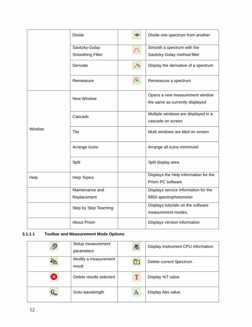
Divide

Divide one spectrum from another

Savitzky-Golay

Smoothing Filter

Smooth a spectrum with the

Savitzky-Golay method filter

Derivate

Display the derivative of a spectrum

Remeasure

Remeasure a spectrum

Window

New Window Opens a new measurement window

the same as currently displayed

Cascade Multiple windows are displayed in a

cascade on screen

Tile Multi windows are tiled on screen

Arrange Icons Arrange all icons minimized

Split Split display area

Help Help Topics Displays the Help information for the

Prism PC software

Maintenance and

Replacement

Displays service information for the

6850 spectrophotometer

Step by Step Teaching Displays tutorials on the software

measurement modes.

About Prism Displays version information

3.1.1.1 Toolbar and Measurement Mode Options

Setup measurement

parameters Display Instrument CPU information

Modify a measurement

result Delete current Spectrum

Delete results selected

Display %T value

Goto wavelength

Display Abs value

13

SECTION 4 – PHOTOMETRIC MEASUREMENT

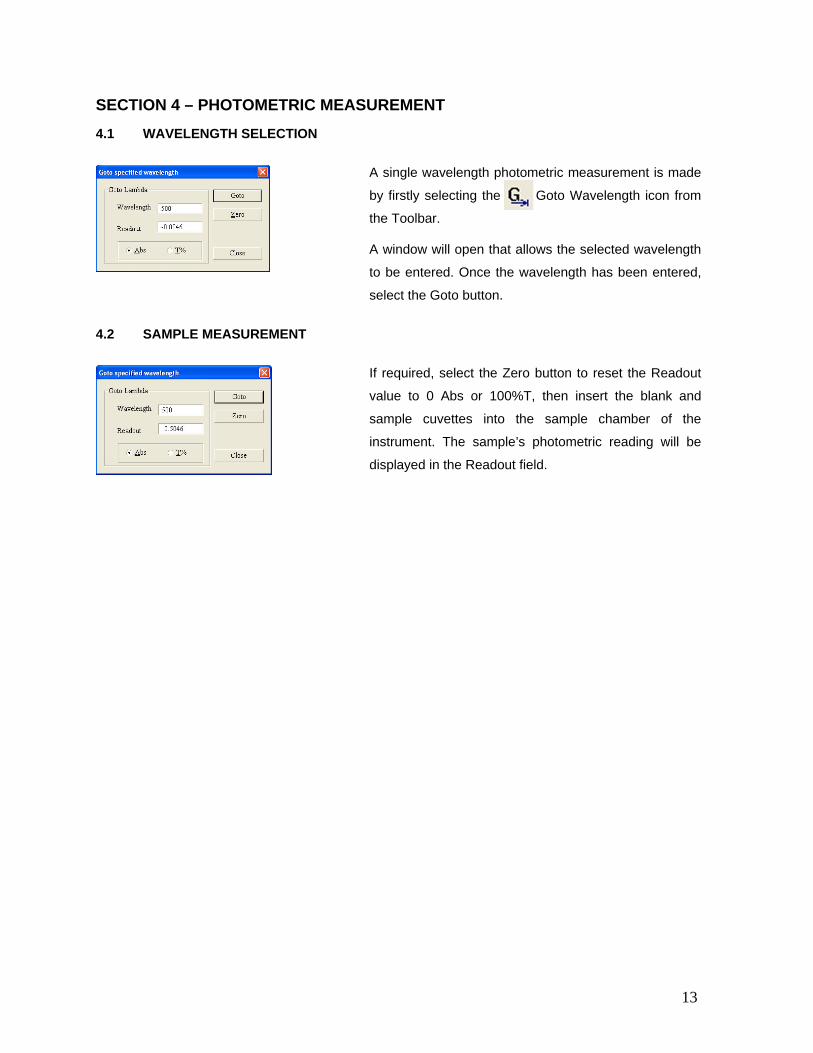
4.1 WAVELENGTH SELECTION

A single wavelength photometric measurement is made

by firstly selecting the Goto Wavelength icon from

the Toolbar.

A window will open that allows the selected wavelength

to be entered. Once the wavelength has been entered,

select the Goto button.

4.2 SAMPLE MEASUREMENT

If required, select the Zero button to reset the Readout

value to 0 Abs or 100%T, then insert the blank and

sample cuvettes into the sample chamber of the

instrument. The sample’s photometric reading will be

displayed in the Readout field.

14

SECTION 5 – MULTIWAVELENGTH / QUANTITATION

The multi wavelength and quantitation measurement mode enables measurements of absorbance, %

transmittance and concentration to be performed. In this measurement mode it is possible to perform

a photometric measurement at up to 20 separate wavelengths. This mode also allows the

concentration of an unknown sample to be determined against a calibration curve or a known

concentration factor at up to three separate wavelengths.

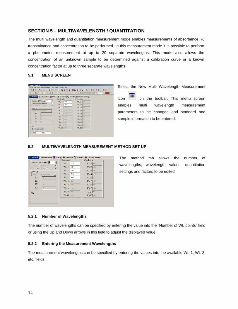
5.1 MENU SCREEN

Select the New Multi Wavelength Measurement

icon on the toolbar. This menu screen

enables multi wavelength measurement

parameters to be changed and standard and

sample information to be entered.

5.2 MULTIWAVELENGTH MEASUREMENT METHOD SET UP

The method tab allows the number of

wavelengths, wavelength values, quantitation

settings and factors to be edited.

5.2.1 Number of Wavelengths

The number of wavelengths can be specified by entering the value into the “Number of WL points” field

or using the Up and Down arrows in this field to adjust the displayed value.

5.2.2 Entering the Measurement Wavelengths

The measurement wavelengths can be specified by entering the values into the available WL 1, WL 2

etc. fields.

15

5.3 SAMPLE INFORMATION

The Information tab allows the user to enter

sample and standard information. Additional

notes can be entered into the Memo field if

required.

5.4 SAMPLE MEASUREMENT AND DISPLAY OPTIONS

The Sample tab contains a result window and a

Control window. The Control window contain

options to Start, Delete, Modify, Recalculate,

change the Data Font and Print.

5.4.1 Control Window – Start

Select the Start button to initiate a

multiwavelength measurement. A new window will

open that displays the measured photometric

values. Once complete, select OK to finish. The

result window will be updated with the measured

values.

5.4.2 Control Window – Delete

Select the Delete button to delete a completed sample measurement.

5.4.3 Control Window - Modify

Select the Modify button to re-measure a sample’s photometric values. The updated values will over-

right any previously recorded data.

16

5.4.4 Control Window – Recalculate

Select the Recalculate button to re-evaluate the concentration result when the Quantitation mode is

enabled.

5.4.5 Control Window – Data Font

Select the Data Font button to format the result data.

5.4.6 Control Window – Print

Select the Print button to generate a report of the recorded data. The user will be asked to confirm if

the report should include the text entered into the Information tab fields and the data contained in the

result window.

5.5 QUANTITATION MEASURMENTS

The Quantitation measurement mode is enabled

by selecting the Method tab and checking the tick

box besides the Calculate Concentration option. If

standard solutions are to be used to construct a

new calibration curve, check the tick box besides

the Use Standard Sample option.

No more than 3 wavelengths can be measured

when the Quantitation mode is enabled.

5.5.1 Using a Concentration Factor or Pre-defined Calibration Curve

If the concentration factor or the calibration curve constants are already known, these values can be

entered into the method settings to allow an unknown sample to be quantified.

5.5.1.1 Entering a Known Concentration Factor

The Use Standard Samples checkbox should be

clear and the Curve Fit option should be set to

Linear Fit. The concentration factor should then

be entered into the K1 field.

17

5.5.1.2 Entering Known Calibration Curve Constants

The Use Standard Samples checkbox should be

clear and the Curve Fit option should be set to

the appropriate option. The known calibration

curve constants should then be entered into the

appropriate K0 – K3 fields where:-

Concentration = (K3*X3)+ (K2*X2)+ (K1*X) + K0

X = Photometric value of the sample

5.5.2 Constructing a New Calibration Curve

To construct a new calibration curve the user

must ensure that they check the tick boxes beside

the Calculate Concentration and Use Standard

Sample options.

5.5.2.1 Measuring Standard Samples

Select the Standard tab.

Insert the first standard into the sample position

in the sample chamber and the reference into the

reference position in the sample chamber.

Select the Start button to initiate the

measurement

A new window will open allowing the Standard

name, final photometric reading and

concentration to be edited. The actual

photometric reading of the standard will be

displayed in the Readout window and this value

will default to the deltaAbs field.

18

Once the standard measurement is complete

and the name and concentration information has

been entered, select OK to transfer the

information to the main standard tab.

Repeat this procedure for each standard sample.

5.5.2.2 Calibration Curve Settings and Display

The calibration curve display settings are edited

by selecting the Display Setting tab.

The calibration curve’s labels, axis range and

interval values and concentration units can be

edited in this tab.

The calibration curve is displayed by selecting

the Fitting tab.

19

5.5.3 Sample Measurement

To quantify an unknown sample select the

Sample tab and select the Start button.

A new window will open allowing the sample

name and final reported photometric reading to

be edited. The actual photometric reading of the

standard will be displayed in the Readout window

and this value will default to the deltaAbs field.

Select OK to transfer the data to the sample

result table.

The sample result table will display the measured

absorbance value, the final reported absorbance

value and the calculated concentration value.

20

SECTION 6 – SPECTRUM

The spectrum measurement mode enables measurements of absorbance or % transmittance over a

range of wavelengths to be performed. The absorbance or % transmittance at each wavelength is

plotted graphically. Post measurement tools such as peaks/valleys, derivatives and spectral points

analysis can be performed. This operating mode can be used to partially characterise a sample.

6.1 SPECTRUM MODE SCREEN

Select the Spectrum Measurement icon on

the toolbar. The Spectrum measurement window

will open.

6.2 METHOD SETUP

The spectrum scan settings can be edited by

selecting the settings icon in the toolbar.

The options that can be changed are:-

1. Scan from (Highest Wavelength)

2. Scan to (Lowest Wavelength)

3. Scan Step (0.5, 1.0, 2.0, 4.0, 5.0nm)

4. Scan Precision (5, 10, 30, 50)

The required options can be entered directly or selected from the available options via the drop down

lists. Select OK to confirm.

6.3 SELECTING THE MEASUREMENT MODE

The required measurement mode can be selected from the available options of Abs and %T by

selecting the or icons on the toolbar.

21

6.4 SAMPLE MEASUREMENTS

Insert a cuvette containing the blank solution into

the reference position in the sample chamber

and insert the cuvette containing the sample

solution into the sample position. Close the

instrument lid and select the Start a

measurement icon on the toolbar. Once the

measurement is complete the measured

spectrum scan will be displayed on the screen.

The scan can be cancelled by selecting the Stop

a measurement icon .

6.5 POST MEASUREMENT TOOLS

6.5.1 Adjusting the Displayed Scan Range

Select the Setup display spectrum icon from

the toolbar. Enter the required display settings

and select OK to confirm.

6.5.2 Spectrum Peaks and Valleys

Select the Peak/Valley Threshold icon from

the toolbar. Enter the required absorbance (peak

height) threshold and select OK to confirm.

Select the identify spectrum peaks icon from

the toolbar to list the peaks information and select

the identify spectrum valleys icon to list the

valley information.

22

6.5.3 Spectrum Zoom Function

Select the Zoom function icon from the toolbar. Position the cursor in the upper-left corner of the

area you want to select. Hold the left mouse button to drag the cursor to outline the spectrum area you

want to enlarge. Release the mouse button. The part of the spectrum which is displayed within the

outlined area will be enlarged. Select the undo zoom icon to restore the previous view settings.

Select the Zoom function icon again to exit the zoom function.

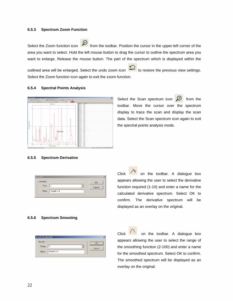
6.5.4 Spectral Points Analysis

Select the Scan spectrum icon from the

toolbar. Move the cursor over the spectrum

display to trace the scan and display the scan

data. Select the Scan spectrum icon again to exit

the spectral points analysis mode.

6.5.5 Spectrum Derivative

Click on the toolbar. A dialogue box

appears allowing the user to select the derivative

function required (1-10) and enter a name for the

calculated derivative spectrum. Select OK to

confirm. The derivative spectrum will be

displayed as an overlay on the original.

6.5.6 Spectrum Smooting


appears allowing the user to select the range of

the smoothing function (2-100) and enter a name

for the smoothed spectrum. Select OK to confirm.

The smoothed spectrum will be displayed as an

overlay on the original.

23

6.5.7 Remeasure (Re-plot) Spectrum


appears asking the user to specify the frequency

of the data points in the re-plotted spectrum.

Select OK to confirm. The re-plotted spectrum

will be displayed.

6.6 OVERLAY SPECTRA

The Prism Pc software can display multiple

spectrum scans simultaneously on the screen by

either measuring additional samples or loading

stored data. The active spectrum is selected from

the drop down menu on the toolbar. The colours

of the selected spectrum’s background and

photometric trace can be selected using the

palette options on the toolbar.

6.6.1 Spectrum Addition, Subtraction, Multiplication and Division

Click , , or on the toolbar.

A dialogue box will appear asking the user to

specify the files to be used in the calculation and

enter a name for the calculated spectrum. Select

OK to confirm. The calculated spectrum will be

displayed.

24

6.6.2 Delete Displayed Spectrum

Select the spectrum to be deleted in the active spectrum drop down box (see 6.6). Click on the

toolbar to remove the spectrum from the display.

6.7 SPECTRUM DISPLAY AND PRINT OPTIONS

The display and print options for the selected

spectrum can be accessed by selecting the

icon on the toolbar. The display range, peak and

valley labels, axis legends, spectrum title, display

colours, print information options and printout

notes can be edited in the dialogue box that

appears.

25

SECTION 7 – KINETICS

The kinetics measurement mode enables the absorbance or % transmittance of an active molecule to

be measured over a period of time; for example enzyme analysis of horseradish peroxidase. The

absorbance or % transmittance is measured at regular time intervals at a set wavelength over a period

of time. The results are plotted on a graph to show the change in absorbance or % transmittance over

time. Following sample measurement statistical analysis of all or part of the experiment can be

performed.

7.1 KINETICS MODE SCREEN

Select the Kinetics Measurement icon

on the toolbar. The Kinetics measurement

window will open.

7.2 METHOD SETUP

The kinetics scan settings can be edited by

selecting the settings icon in the toolbar.

The options that can be changed are:-

1. Scan wavelength

2. Scan time (max 100000s)

3. Scan Step (0.1, 0.2, 0.5, 1.0, 2.0,

5.0, 10.0, 30.0, 60.0s)

The required options can be entered directly or selected from the available options via the drop down

lists. Select OK to confirm.

7.3 SELECTING THE MEASUREMENT MODE

The required measurement mode can be selected from the available options of Abs and %T by

selecting the or icons on the toolbar.

26

7.4 SAMPLE MEASUREMENTS

Insert a cuvette containing the blank solution into

the reference position in the sample chamber

and insert the cuvette containing the sample

solution into the sample position. Close the

instrument lid and select the Start a

measurement icon on the toolbar. Once the

measurement is complete the measured

spectrum scan will be displayed on the screen.

The scan can be cancelled by selecting the Stop

a measurement icon .

7.5 POST MEASUREMENT TOOLS

7.5.1 Adjusting the Displayed Scan Range

Select the Setup display spectrum icon from

the toolbar. Enter the required display settings

and select OK to confirm.

7.5.2 Kinetics Zoom Function

Select the Zoom function icon from the toolbar. Position the cursor in the upper-left corner of the

area you want to select. Hold the left mouse button to drag the cursor to outline the scan area you

want to enlarge. Release the mouse button. The part of the scan which is displayed within the outlined

area will be enlarged. Select the undo zoom icon to restore the previous view settings. Select

the Zoom function icon again to exit the zoom function.

27

7.5.3 Spectral Points Analysis

Select the Scan spectrum icon from the

toolbar. Move the cursor over the kinetics

spectrum to trace the scan and display the scan

data. Select the Scan spectrum icon again to exit

the spectral points analysis mode.

7.5.4 Kinetics Derivative


appears allowing the user to select the derivative

function required (1-10) and enter a name for the

calculated derivative spectrum. Select OK to

confirm. The derivative spectrum will be

displayed as an overlay on the original.

7.5.5 Remeasure (Re-plot) Kinetics Scan


appears asking the user to specify the frequency

of the data points in the re-plotted kinetics scan.

Select OK to confirm. The re-plotted kinetics

scan will be displayed.

7.6 OVERLAY SCANS

The Prism Pc software can display multiple

kinetics scans simultaneously on the screen by

either measuring additional samples or loading

stored data. The active kinetics scan is selected

from the drop down menu on the toolbar. The

colours of the selected scan’s background and

photometric data can be selected using the

palette options on the toolbar.

28

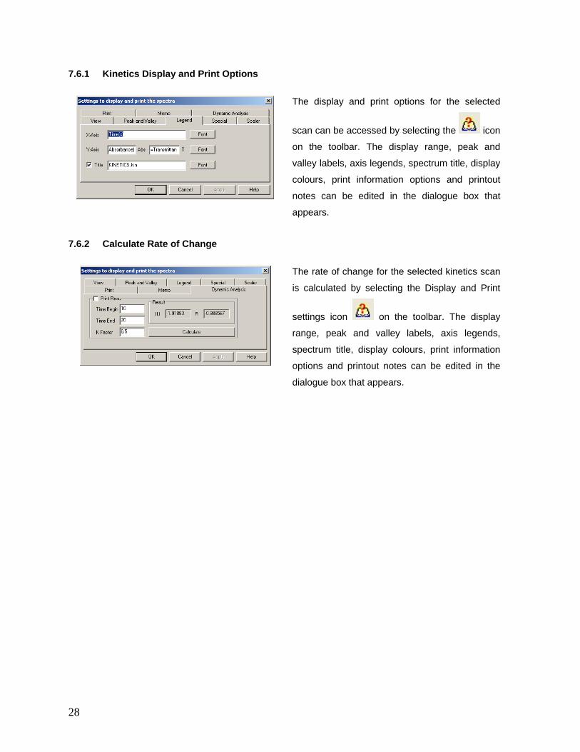
7.6.1 Kinetics Display and Print Options

The display and print options for the selected

scan can be accessed by selecting the icon

on the toolbar. The display range, peak and

valley labels, axis legends, spectrum title, display

colours, print information options and printout

notes can be edited in the dialogue box that

appears.

7.6.2 Calculate Rate of Change

The rate of change for the selected kinetics scan

is calculated by selecting the Display and Print

settings icon on the toolbar. The display

range, peak and valley labels, axis legends,

spectrum title, display colours, print information

options and printout notes can be edited in the

dialogue box that appears.

29

SECTION 8 – DNA/PROTEIN

The DNA/Protein measurement mode allows the user to measure multi-wavelength absorbance ratios,

such as 260nm/280nm and 260nm/230nm, which are commonly used to estimate a protein or nucleic

acid sample’s purity. The mode also includes calculations that can be used to estimate the

concentration of the protein or nucleic acid sample.

Four commonly used protein assay methods are pre-loaded in this measurement mode. The available

protein assay methods are Direct UV, Lowry, Bradford, Biuret and BCA.

8.1 DNA/PROTEIN MODE SCREEN

Select the DNA/Protein Measurement icon

on the toolbar. The DNA/Protein measurement

window will open.

8.2 METHOD SETUP

The DNA/Protein method options are selected

from the Method drop down box. The methods

that are available are:-

1. 260/280

2. 260/230

3. UV Method

4. Lowry

5. BCA

6. Bradford

7. Biuret

8.2.1 Adjusting the Method Parameters

Select the DNA/Protein Measurement field to

edit and enter the required wavelength or

concentration factor. The displayed

concentration unit is selected from the Unit drop

down menu.

30

8.3 DETERMINATION OF NUCLEIC ACID CONCENTRATION

Select the required method parameters as in 8.2.

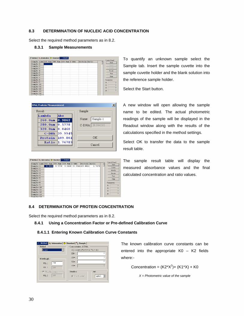
8.3.1 Sample Measurements


Sample tab. Insert the sample cuvette into the

sample cuvette holder and the blank solution into

the reference sample holder.

Select the Start button.


name to be edited. The actual photometric

readings of the sample will be displayed in the

Readout window along with the results of the

calculations specified in the method settings.


result table.

The sample result table will display the

measured absorbance values and the final

calculated concentration and ratio values.

8.4 DETERMINATION OF PROTEIN CONCENTRATION

Select the required method parameters as in 8.2.

8.4.1 Using a Concentration Factor or Pre-defined Calibration Curve

8.4.1.1 Entering Known Calibration Curve Constants

The known calibration curve constants can be

entered into the appropriate K0 – K2 fields

where:-

Concentration = (K2*X2)+ (K1*X) + K0

X = Photometric value of the sample

31

8.4.2 Constructing a New Calibration Curve

8.4.2.1 Measuring Standard Samples

Select the Standard tab.

Insert the first standard into the sample position in

the sample chamber and the reference into the

reference position in the sample chamber.

Select the Start button to initiate the measurement

A new window will open allowing the Standard

name and concentration to be edited. The actual

photometric reading of the standard will be

displayed in the Readout window. Select OK to

transfer the information to the main standard tab.

Repeat this procedure for each standard sample.

8.4.3 Sample Measurement


Sample tab and select the Start button.

32


name to be edited. The actual photometric

reading of the standard will be displayed in the

Readout window and this value will default to the

C-DNA field.


result table.

The sample result table will display the measured

absorbance value and the calculated

concentration value.

33

SECTION 9 – APPENDIX

The multicell accessory measurement mode allows the user to measure a sample’s photometric

absorbance or %transmittance at up to 10 wavelengths. Following sample measurement, the

photometric readings are displayed on the multi-wavelength mode screen.

9.1 CALCULATIONS IN QUANTITATION MODE

Single Wavelength Method ：Abs.=A1

Double Wavelengths Method ：Abs.=m*A1-n*A2

Three Wavelengths Method ：Abs.=A1-(WL1-WL2)*(A2-A3)/(WL2-WL3)-A3

9.2 CALCULATIONS IN DNA/PROTEIN MODE

260/280: CDNA =(A1-Aref)*f1-(A2-Aref)*f2 CProtein =(A2-Aref)*f3-(A1-Aref)*f4 Ratio =(A1-Aref)/(A2-Aref)

A1=A260nm, A2=A280nm, Aref=A320nm (Optional)

f1=62.9, f2=36.0, f3=1550, f4=760.0 260/230: CDNA =(A1-Aref)*f1-(A2-Aref)*f2

CProtein =(A2-Aref)*f3-(A1-Aref)*f4 Ratio =(A1-Aref)/(A2-Aref)

A1=A260nm, A2=A230nm, Aref=A320nm (Optional)

f1=49.1, f2=3.48, f3=183, f4=75.8

34

SECTION 10 – TECHNICAL SUPPORT

10.1 TECHNICAL SUPPORT

Jenway have a dedicated Technical Support team made up of experienced scientists who are on hand

to help with any applications advice and questions you may have about our products and how to use

them. If you require any technical or application assistance please contact the team at:

E-mail: [email protected].

Phone: +44 (0)1785 810433

Fax: +44 (0)1785 810405

Jenway PRISM PC Software · 4 SECTION 1 – Introduction 1.1 PC SOFTWARE DESCRIPTION The Prism PC...

Documents

Transcript of Jenway PRISM PC Software · 4 SECTION 1 – Introduction 1.1 PC SOFTWARE DESCRIPTION The Prism PC...