
Jensen, J. R. 2005. Introductory Digital Image Processing...
99
• Jensen, J. R. 2005. Introductory Digital Image Processing (3 rd edition). Prentice Hall.
Transcript of Jensen, J. R. 2005. Introductory Digital Image Processing...

• Jensen, J. R. 2005. Introductory Digital Image Processing (3rd edition). Prentice Hall.

General Questions
• Where and when has change taken place in the landscape?
• How much change, and what type of change has occurred?
• What are the cycles and trends in the change?

Types of Change Detection
• Between-class changes– Based on classification imagery
– Answers the question, “Has a pixel changed and what has it changed to?”
– e.g. forest to agriculture conversion
• Within-class changes– Based on continuous spectral or transformed spectral
information
– Answers the question, “How much and in what direction has a pixel changed?”
– e.g. change in % vegetation cover

Types of Change Detection
• Use of time as an implicit variable
– The actual time differences are not used in the analysis, just the fact that two images are from different times.
• Use of time as an explicit variable
– If we are interested in the amount of change/unit time, we need to include time explicitly in our analyses.

Change Detection Process
Data Acquisition and Preprocessing
Radiometric/Geometric Correction
Data Normalization
Change Detection Analysis
Accuracy Assessment
Final Product Generation

Change Detection Analysis
• Landscape is dynamic
• Allows for the monitoring of change over time -Rates e.g., x % per year deforestation- Amounts e.g., x km2 loss of wetlands
• General steps to perform digital change detection are shown next


• To map patterns of forest change, specifically deforestation,
• To analyze the rates of such changes in the tropics and elsewhere
• Monitoring of change is frequently perceived as one of the most important contributions of remote sensing technology to the study of global ecological and environmental change.
• Land cover changes can occur in two forms: - conversion of land cover from one category to a completely different category (via
agriculture, urbanization, etc.), - modification of the condition of the land cover type within the same category
(thinning of trees, selective cutting, etc.)
Why do change analysis?


Change detection
1982-1992 land use change
29,860 acres/year
1992-1995 land use change
56,640 acres/year
% total non-federal land developed– 1982 = 27.7%– 1985 = 32.7%– 1992 = 34.4%– 1997 = 40.8%

Products of Change Detection• Change area and rate• assessing the spatial pattern of the change • Change trajectories; identifying the nature of the change• Accuracy assessment of change detectionresults

Change-Detection Considerations• Precise geometric registration• Radiometric normalization/calibration• Phenology, soil moisture, sun angles (select images of similar solar days)• Image complexity of the study area and mixeleffects (use images of similar spatial resolutions)• Compatibility of images from different sensors• Classification and change detection schemes(application oriented – change/non-change vs changedirections)• Change detection methods• Ground truth data• Analyst’s skill and experience• Time and cost restrictions

Before implementing change detection analysis, the following conditions must be satisfied:(1) precise registration of multi-temporal images; (2) Precise radiometric and atmospheric calibration or normalization between multi-temporalimages; (3) similar phenological states between multi-temporal images; and (4) selection of the same spatial and spectral resolution images if possible.

Temporal Resolution
• When performing change detection using RS data from multiple dates, two temporal resolutions must be held constant for optimal results:
1. Data should be acquired the same time of day (e.g., Landsat TM is before 9:45 am in U.S.)
2. Data should be collected on anniversary dates (removes sun angle & plant phenological differences)

Spatial Resolution & Look Angle
• Accurate spatial registration of at least two images is essential for optimal digital change detection. Ideally the following should be held constant:– Data collected with the same Instantaneous-
Field-Of-View (IFOV) i.e., same pixel size
– Rectification Root Mean Square Error (RMSE) of < 0.5 of a pixel i.e., reduce misregistration
– Data collected from the same look angle i.e.reduce reflectance differences

Spectral Resolution
• Data should be collected from the same sensor in the same bands
– This achieves the best results but when this is not possible, bands which most closely approximate one another should be used.

Radiometric Resolution
• Data should be collected at the same radiometric precision on both dates– When the radiometric resolution of data
acquired by one system are compared with data acquired by a higher radiometric resolution instrument (e.g., Landsat TM with 8-bit data) then the lower resolution (e.g., 6-bit data) should be decompressed to 8-bits for change detection purposes. Note: precision of decompressed brightness values is not as good as original, uncompressed data.

Environmental Considerations
• When performing change detection it is also desirable to hold environmental variables such as:
– Atmospheric
– Soil
– Vegetative
conditions as constant as possible

Atmospheric Conditions
• Ideal atmospheric conditions for the collection of remotely sensed data include no clouds, haze, or extreme humidity.
• Cloud cover > 20% is usually considered unacceptable.
• If dramatic differences exist in atmospheric conditions across the imagery to be used then atmospheric attenuation in the imagery must be corrected for e.g., using in situ data and atmospheric transmission models or alternate empirical methods.

Soil Moisture Conditions
• Under ideal conditions, soils moisture should be identical across dates.
• This means the dates for imagery must be reviewed before purchase to compare precipitation records in the days and weeks prior to the image date.

Vegetative Conditions
• Similar times of year and moisture conditions usually result in similar phenological stages in vegetation. Hence if the other conditions are met in terms of environmental and resolution considerations, usually vegetative conditions are also.
• Ground data should be available to confirm changes in vegetation, which is usually what we are studying with change detection.

Images must undergo a number of restoration steps that involve radiometric calibration, atmospheric correction, and radiometric rectification to ensure we are obtaining real image differences in our change detection
These processes remove differences between the images related to:
- sensor differences (intra-instrument differences,
instrument drift, or inter-instrument differences),
- illumination differences (earth-sun distances, solar incidence
angle),
- atmospheric differences (aerosol content, water droplet
concentration)
Calibration Procedures

Radiometric Calibration/Normalization1. Absolute correction/calibration:• Converting from DN to ground reflectance (or radiance) using atmospheric models
2. Relative normalization:• Based on regression or histogram matching techniques to register the radiometric signals of one image to another. • Noise reduction• Haze reduction

Change Detection: Radiometric Calibration
• Histogram matching
Band 4
Pix
el C
ou
nt

Change Detection: Radiometic Calibration
• Regression Approach
Band 4, 1999
Ban
d 4
, 19
88
Dark Objects
Light Objects

Change Detection
• Atmospheric correction
– Model atmospheric effects using radiative transfer models
• Aerosols, water vapor, absorptive gases

Atmospheric Correction Necessary / Not Necessary
• NECESSARY: Required when individual date images used in change detection algorithm are based on linear transformation of data, a normalized difference of vegetation index image is produced
• NECESSARY: Imagery should be atmospherically corrected if the change detection is based on multiple-date red/near-infrared ratio images (landsat tm 4 / landsat tm 3)
• UNNECESSARY: It is unnecessary to correct for atmospheric effects prior to image classification if the spectral signatures characterizing the desired classes are derived from the image to be classified – images from a single date. – It is not necessary to atmospherically correct Landsat TM data obtained on Date 1 if it is going to be
subjected to a maximum likelihood classification algorithm and all the training data are derived from the Date 1 imagery. The same hold true when a Date 2 image is classified using training data extracted from the Date 2 image. Change between the Date 1 and Date 2 classification maps derived from the individual dates of imagery (corrected or uncorrected can easily be compared in post-classification comparison.
• UNNECESSARY: It is also unnecessary when change detection is based on classification of multiple date composite imagery in which the multiple dates of remotely sensed imaged are rectified and placed in a single dataset and then classified as if it were a single image (e.g. multiple date principle components change detection).
• NECESSARY: Only when Training data from one time and/or place are applied in another time and/or place is atmospheric correction necessary for image classification and many change detection algorithms.

Some examples of Change Detection and Analysis
• Classification Algorithms (after Jensen 2005)1. Direct Comparison – “Blinking”2. Write Function Memory Insertion3. Multi-Date Composite Image4. Image Algebra Change Detection5. Post-classification Comparison6. Multi-date Change with Binary Mask7. Multi-date Change with Ancillary Data8. Manual, On-screen Digitizing9. Spectral Change Vectors10. Knowledge-Based Vision Systems
• Index Algorithms - Thresholding

Change Detection: Methods
• Basic model:
– Inputs:
• Landsat TM image from Date 1
• Landsat TM image from Date 2
– Potential output:
• Map of change vs. no-change
• Map describing the types of change

Change Detection: Methods
• Display bands from Dates 1 and 2 in different color guns of display
– No-change is greyish
– Change appears as non-grey
• Limited use
– On-screen delineation
– Masking

Direct: “Blinking”Link two composites, “blink” back and forth.
Advantages:Simple and Immediate.
Disadvantages:No change class labels, to-from analysis,


Write-Function Memory Insertion
(RGB Control)
R = Band 4 1975G = Band 4 1986B = Band 4 1986


Multi-date Composite Image Change Detection in Imagine
PCA
PC 1
PC 2
PC 3
Composite


Image Algebra Change Detection in Imagine

Image Algebra Change Detection in Imagine
Red = > 20% decrease; Green = > 20% increase in Band 4
Based on non-corrected Digital Numbers
Difference Image, mean -26

Thresholding
Standard Normal Deviates
Z = ( x – x ) / s.d.
Z = (x - 0.038) / 0.114
Threshold = + 2 s.d.


Change Detection: Methods
• Image differencing
– Date 1 - Date 2
– No-change = 0
– Positive and negative values interpretable
– Pick a threshold for change
– Often uses vegetation index as start point, but not necessary

Image Differencing
8 10 8 11
240 11 10 22
205 210 205 54
220 98 88 46
5 9 7 10
97 9 8 22
98 100 205 222
103 98 254 210
3 1 1 1
143 2 2 0
107 110 0 -168
117 0 -166 -164
Image Date 1
Image Date 2Difference Image = Image 1 - Image 2

Change Detection: Methods
• Image differencing: Pros– Simple (some say it’s the most commonly used method)
– Easy to interpret
– Robust
• Cons:– Difference value is absolute, so same value may have
different meaning depending on the starting class
– Requires atmospheric calibration for expectation of “no-change = zero”

Image Differencing
Shadow Fraction, 1986 Shadow Fraction, 2002
Roads

Image Differencing
• Shadow difference image = Shadow image (2002) -Shadow image (1986)
• Loss of shadow (darker pixels) is related to clearings, gain of shadow (brighter pixels) is related to forest recovery.
Roads

Image Differencing

Image Differencing
• If we use a change threshold of 1 stdev, we can classify the image into gain, no-change or loss.
• Red signifies loss of shadow (loss of forest), green gain of shadow (forest recovery), black no-change.
Helipads
Roads

Change Detection: Methods
• Image Ratioing
– Date 1 / Date 2
– No-change = 1
– Values less than and greater than 1 are interpretable
– Pick a threshold for change

Change Detection: Methods
• Image Ratioing: Pros
– Simple
– May mitigate problems with viewing conditions, esp. sun angle
• Cons
– Scales change according to a single date, so same change on the ground may have different score depending on direction of change; I.e. 50/100 = .5, 100/50 = 2.0

Change DetectionImage Difference (TM99 – TM88) Image Ratio (TM99 / TM88)

Multi-date Change Detection Using A
Binary Mask Applied to Date 2
- very effective method
- Date1 –base image
- Date 2- earlier image or later
image
- spectral change image is then
recorded in to binary mask file

Change Vector Analysis (CVA)
Change Vector Analysis (CVA) uses two spectral channels to map both the: 1) magnitude of change and, 2) the direction of change between the two (spectral) input images for each date.

Change Detection: Methods
• Change vector analysis
– In n-dimensional spectral space, determine length and direction of vector between Date 1 and Date 2
Band 3
Ban
d 4
Date 1
Date 2

Change Detection: Methods
• No-change = 0 length
• Change direction may be interpretable
• Pick a threshold for change

Change Vector AnalysisBand Math followed by change vector
2-D change vector
3-D change vector


•EXAMPLE CVA: The first step of the example CVA method was to apply a Tasseled Cap transform which generates the components Greenness and Brightness, in order to reduce the amount of redundant information of orbital images to be analyzed. This transform can be understood as defining a new coordinate system, where data from different bands occupy a new system of coordinates, where data from the different bands occupy new axes associated with biophysical properties of targets. In this case, such axes are Greenness, associated with the amount and vigor of vegetation, and Brightness, associated with variations of soil reflectance.
•The position variation of the same pixel during different data-takes within the space formed by these two axes, determines the magnitude and direction of the spectral change vectors.
•The next step in the band transformation process into new coordinates axes was to calculate the magnitude of variation among spectral change vectors between the images pairs.
•The magnitude of vectors was calculated from the Euclidean Distance between the difference in positions of the same pixel from different data-takes within the space generated by the axes Greenness and Brightness, as follows:


Change Detection: CVA Methods
• Change detection: Pros
– Conceptually appealing
– Allows designation of the type of change occurring
• Cons
– Requires very accurate radiometric calibration
– Change value is not referenced to a baseline, so different types of change may have same change vector

Example of Change Vector Analysis: Tugend 2001: Lake Kissimmee Littoral Zone “Enhancement”
Decreases in brightness of bands 1, 2, 3 due to increases of vegetation.Increases in brightness due either to decrease of vegetation, or increases of turbidity.

• A useful vegetation or greenness index can be created from a ratio of the visible and near-infrared data, known as the normalized difference vegetation index (NDVI) (Campbell, 1996).
• This index can be used to show the amount of vegetation present at a given time, and can be used in change analyses to indicate how a landscape changes in terms of vegetation amount across a set time period.
• Quite simply we can subtract one image from a second image
e.g., 1990 NDVI – 1980 NDVI = A number > 0.0 means an increase in vegetation since 1980
Vegetation Indices in Change Detection

Figure 4: Frequency of NDVI change values across the La Campa-Gracias image region
0
5000
10000
15000
20000
25000
30000
35000
40000
-1.33 -1.21 -1.08 -0.95 -0.83 -0.70 -0.57 -0.44 -0.32 -0.19 -0.06 0.06 0.19 0.32 0.44 0.57 0.70 0.82
1996 NDVI pixel value - 1987 NDVI pixel value (above 0.0 means increasing vegetation)
Fre
qu
en
cy
of
pix
els
0.0 (no change in vegetation)
Decreasing vegetation amount Increasing vegetation amount
Frequency of NDVI change values across the La Campa & Gracias study area

Change Detection: Methods
• Post-classification (delta classification)
– Classify Date 1 and Date 2 separately, compare class values on pixel by pixel basis between dates


Post-Classification Change Comparison
Use “confusion matrix” as a to-from change matrix.
1997 – “Classified”1994 – “Ground Truth”
LegendClass 1 = BlueClass 2 = GreenClass 3 = RedClass 4 = YellowClass 5 = Cyan

Change Detection: Methods
• Post-classification: Pros
– Avoids need for strict radiometric calibration
– Favors classification scheme of user
– Designates type of change occurring
• Cons
– Error is multiplicative from two parent maps
– Changes within classes may be interesting


Change Detection: Methods
• Composite Analysis
– Stack Date 1 and Date 2 and run unsupervised classification on the whole stack

Composite Analysis
Steps
1. Geometrically correct images.
2. Merge the images into a single image.• The number of bands in the composite image typically = the number
of bands in a single image x the number of images used.
• e.g. if we use 2 MSS images, the composite images will have 4 bands x 2 image = 8 bands.
3. We use the composite image to perform classification. “Change” categories should be statistically different from “no change” categories.

Composite Analysis
Benefits
• Only a single classification is needed.
• May extract maximum change variation
• Includes reference for change, so change is anchored at starting value, unlike change vector analysis and image differencing
Drawbacks
• Class choices and interpretation can be complex. This is more of a classification technique that takes change into consideration, than a true change-detection technique.

Principle Components Analysis
Steps
1. Geometrically correct images.
2. Perform PCA transformation.
3. Interpret PCA images (each image will contain a single axis).

Principle Components Analysis
PCA Axis 1
PCA Axis 3
PCA Axis 2
PCA Axis 4

Principle Components Analysis
Benefits
• Relatively easy to do, can reduce a large dataset into a much smaller dataset.
Drawbacks
• Interpretation can be difficult.

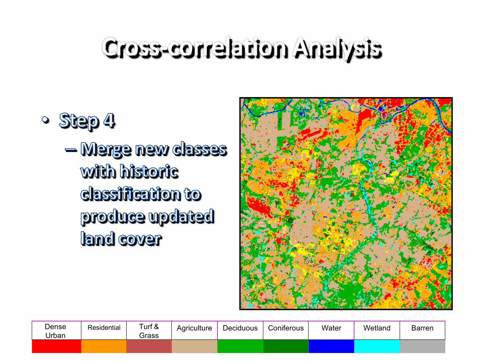
Cross-Correlation Analysis (CCA)
Cross-Correlation Analysis (CCA) uses a land cover map to delineate spectral cluster statistics between the baseline image year (Time 1) and each scene in the temporal sequence (Time 2). Calculating the Z-statistic deviations from the cluster mean identifies change pixels within each land cover cluster.

2
1 ..
n
i i
ii
DevStd
ExpectedObservedZ
• Z is the distance measure• Observed is the pixel value for each band• Expected is the mean value of all extracted pixels for each band• Std. Dev. Is the standard deviation of all extracted pixels for each band

September 23, 1999
1989 Deciduous Category

Probable
unchanged
Probable
changed
1989 Deciduous Category
Z-values range from 1 to 5,794

Deciduous ConiferousTurf & Grass Agriculture &
Barren

WaterConiferousDeciduousAgricultureTurf &
GrassResidentialDense
UrbanWetland Barren
WaterConiferousDeciduousAgricultureTurf &
GrassResidentialDense
UrbanWetland Barren

Site 1

Site 2

Theil-Sen Regression Analysis (TSA)
Much like typical image regression change, we use Theil-Sen as it is more robust to sample outliers than ordinary least-squares regression.
•Medians are outlier resistant measures of central tendency and the method uses the median of all pairwise slopes to calculate the slope of the regression line.
•The median value of the sample offsets represents the intercept.

TSA con’t…•Generate mask to sample pixels in each land cover•Samples are used to build a regression equation for each cover type using the baseline data as the regressor and each scene in the temporal sequence as the response.
• A change mask is created by mapping pixels characterizing large residuals away from the regression line


Change Detection: Summary
• Radiometric, geometric calibration critical
• Minimize unwanted sources of change (phenology, sun angle, etc.)
• Differencing is simple and often effective
• Post-classification may have multiplicative error
• Better to have a reference image than not


![[PPT]Image Processing - IDC · Web viewFundamentals of Digital Image Processing Anil K. Jain Prentice Hall, 1989. ----- About the course Goals of this course: Introductory course:](https://static.fdocuments.in/doc/165x107/5adff7017f8b9af05b8d14a0/pptimage-processing-viewfundamentals-of-digital-image-processing-anil-k-jain.jpg)
