1

Jean-Pierre Kenné 1 , Pierre Dejax 2 and Ali Gharbi 3

1Mechanical Engineering Department, Laboratory of Integrated Production Technologies, University of Quebec,

École de technologie supérieure, 1100, Notre Dame Street West, Montreal (Quebec), Canada, H3C 1K3 2

Department of Automatic Control and Industrial Engineering, Logistics and Production Systems Group, Ecole des

Mines de Nantes, IRCCyN, BP 20722 - 44307 Nantes Cedex 3 - France 3

Automated Production Engineering Department, Production Systems Design and Control Laboratory, University

of Quebec, École de technologie supérieure, 1100, Notre Dame Street West, Montreal (Quebec), Canada, H3C 1K3

Abstract

This paper deals with the production planning and control of a single product involving combined manufacturing

and remanufacturing operations within a closed-loop reverse logistics network with machines subject to random

failures and repairs. While consumers traditionally dispose of products at the end of their life cycle, recovery of the

used products may be economically more attractive than disposal and remanufacturing of the products also pursue

sustainable development goals. Three types of inventories are investigated in this paper. The manufactured and

remanufactured items are stored in the first and second inventories. The returned products are collected in the third

inventory and then remanufactured or disposed of. The objective of this study is to propose a

manufacturing/remanufacturing policy that would minimise the sum of the holding and backlog costs for

manufacturing and remanufacturing products. The decision variables are the production rates of the manufacturing

and the remanufacturing machines. The Optimality conditions are developed using the optimal control theory based

on stochastic dynamic programming. A computational algorithm, based on numerical methods, is used for solving

the optimal control problem. Finally, a numerical example and a sensitivity analysis are presented to illustrate the

usefulness of the proposed approach. The structure of the optimal control policy is discussed depending on the value

of costs and parameters and extensions to more complex reverse logistics networks are discussed.

Key words: Reverse logistics, closed-loop supply chains, manufacturing/remanufacturing,

optimal control, production Planning, stochastic dynamic programming, Numerical methods.

1. Introduction

The management of return flows induced by the various forms of reuse, or recovery of

products and materials in industrial production processes has received growing attention

throughout the last two decades among practitioners as well as scientists. This is due to the

constant search for increased productivity, a better service to clients, as well as environmental

© 2012. This manuscript version is made available under the CC-BY-NC-ND 4.0 license http://creativecommons.org/licenses/by-nc-nd/4.0/DOI : 10.1016/j.ijpe.2010.10.026

Accepted in International Journal of Production Economics, Vol. 135, No. 1, 2012

Production planning of a hybrid manufacturing/remanufacturing

system under uncertainty within a closed-loop supply chain

2

concerns and the goals of sustainable development in general. Work in this area may be found as

early as the 1900’s. As an example, Amezquita and Bras (1996) analyzes the remanufacturing of

an automobile clutch and Lund (1996) edited a comprehensive report on the remanufacturing

industry. According to the American Reverse Logistics Executive Council, “Reverse logistics

can be viewed as the process of planning, implementing and controlling the efficient, cost

effective flow of raw materials, in-process inventory, finished goods and related information,

from the point of consumption back to the point of origin, for the purpose of recapturing their

value or proper disposal” (Rogers and Tibben-Lembke, 1998).

As mentioned in Fleischmann et al. (1997), reverse logistics encompasses the logistic

activities all the way from used products no longer required by the user to products again usable

in a market. There is a major distinction between material recovery (recycling) and added value

recovery (repair, remanufacturing). They describe the general framework of Reverse

distribution, composed of the “Forward channel” (going from the suppliers and through the

producers and distributors to the consumers, and of the “Reverse channel”, going back from the

consumers through collectors and recyclers, to the suppliers or producers. In all cases, the reuse

opportunities give rise to a new material flow from the user back to the sphere of producers. The

management of this material backward flow opposite to the conventional forward supply chain

flow is the concern of the recently emerged field of «reverse logistics».

Reverse logistics systems have been classified into various categories depending on the

characteristics that are emphasized. Thus several classifications may be found in the literature:

Seaver (1994) focuses on design considerations for the different types of recovery operations

based upon the Xerox Corporation experience; Fleischmann et al. (1997) propose a

comprehensive review of quantitative approaches and distinguish the types of returned items;

Rogers and Tibben-Lembke (1998) analyze trends and practices; Thierry et al. (1995) analyze

the main options for recovery. Theses authors distinguish two categories or reverse logistic

systems and four types or return items or services. The two categories of reverse logistic systems

are open and closed-loop systems, depending on whether the return operations are integrated or

not with the initial operation. The four categories of return items or services are the following:

reusable items (such as returned products or pallets), repair services (where the products are sent

3

back to the consumer after repair), remanufacturing, an industrial process in which used, end of

life products are restored to like-new conditions and put back into the distribution system like the

“new products” and the recycling of raw materials and wastes.

Many case studies and papers proposing models have been published in the area of reverse

logistics as well as several reviews. See De Brito et al. (2003) for a review of case studies;

Dekker et al. (2004) for a review of quantitative models for closed-loop supply chains; Geyer

and Jackson (2004) propose a framework to help identify and assess supply loop constraints and

strategies and they apply it to the recycling and reuse of structural steel Sections in the

construction sector; and Bostel et al. (2005) for a review of optimization models in terms of

strategic, tactical and operational planning. Special issues of journals have been devoted to the

area of reverse, or closed-loop logistics: Verter and Boyaci (2006) edited a special issue journal

on optimization models for reverse logistics. Guide and Van Wassenhove (2006, Part 1 and Part

2) edited a two parts feature issue journal on Closed-Loop Supply Chains.

As can be seen from the numerous published literatures on reverse logistics, many industrial

cases have been reported and many scientific planning or optimization models have been

proposed. These cases and models differ by numerous characteristics. One of the the most

complex situation is found in remanufacturing activities. Traditional areas for remanufacturing

are the automotive or aeronautic sectors (machinery and mechanical assemblies such as aircraft

engines and machine tools) as well as the remanufacturing of toner cartridges (see the report by

Lund (1996) about the remanufacturing industry. An example is Hewlett-Packard, which collects

empty laser-printer cartridges from customers for using again (Jorjani et al. (2004)). Other

examples are described in the next Section.

Individual repair requirements for every product returned, and coordination of several

interdependent activities makes production planning a highly sophisticated task in this

environment. In contrast with traditional manufacturing systems (forward direction), no well-

determined sequence of production policies exist in remanufacturing (backward or reverse

direction). This is illustrated by Sundin and Bras (2005) who describes a model of

4

remanufacturing steps not following a specific order. In many cases, the original manufacturer is

also in charge of collecting, refurbishing, and remanufacturing the used products.

The production planning in a hybrid context, involving manufacturing and remanufacturing

facility, referred to as forward-reverse logistics in a closed-loop network, is very complex

especially in the presence of uncertainties and under the consideration of the overall system’s

dynamics. Much of the work in the area of remanufacturing is devoted to the strategic design of

the closed-loop system, or to the tactical or operational planning of production and management

of inventories, considering discrete periods of time. See the next Section for a more

comprehensive review of literature related to the remanufacturing activities.

In this paper we address the area of an integrated combined manufacturing / remanufacturing

within a closed-loop supply chain subject to uncertainties. We study the production planning of a

hybrid manufacturing/remanufacturing system in a dynamic continuous time stochastic context.

Uncertainties are due to machine failures and continuous time modeling seems to us a better

framework to consider stochastic aspects. We found no such approach in the published literature

on remanufacturing. We develop a generic stochastic optimization model of the considered

problem with two decision variables (production rates of manufacturing and remanufacturing

machines) and two state variables (stock levels of manufactured and remanufactured products).

Our goal is to characterize optimal policies for the production rates of the new products as well

as the remanufactured products, depending on the values of the model parameters and costs.

Our modeling approach could possibly be applied to many industrial cases such as those

mentioned in this Section or the next where machines can be subject to failures and their

production rates can be continuously controlled. We feel the assumptions made can be

acceptable, at least approximately, in many cases, but this should be verified as the first step of

an industrial application. It is assumed in particular that the remanufactured products can be

considered meeting the same quality level as the new products so that both type of products can

be distributed like new. We also assume that the demand for new products is deterministic and

known in advance and the proportion of returned products to be possibly remanufactured is a

known proportion of demand. A typical example might be the remanufacturing of copier

cartridges, or aeronautical parts.

5

The rest of the paper is organised as follows. In Section 2, the literature review is presented.

The model notations, the assumptions and the control problem are presented in Section 3. A

numerical example and a sensitivity analysis (carried out to analyse the effect of the used

products return ratio and the backlog costs), are given in Sections 4 and 5, respectively.

Discussions and the direction for future works are presented in Section 6. The paper concludes

with a short summary in Section 7.

2. Literature review

In this Section, we focus on cases and models related to remanufacturing activities. A

number of practical cases have been reported in various contexts of application. Many works are

devoted to the design of the network system or to production or inventory planning through

discrete optimization models.

De Brito et al (2003) discuss network structures and report cases pertaining to the design of

remanufacturing networks by the original equipment manufacturers or independent

manufacturers, the location of remanufacturing facilities for copiers, especially Canon copiers

and other equipments and the location of IBM facilities for remanufacturing in Europe. They

also present case studies on inventory management for remanufacturing networks of engine and

automotive parts for Volkswagen and on Air Force depot buffers for disassembly,

remanufacturing and reassembly. Finally, they present case studies on the planning and control

of reverse logistics activities, and in particular inventory management cases for remanufacturing

at a Pratt & Whitney aircraft facility, yielding decisions of lot sizing and scheduling.

As mentioned above their survey on design, planning and optimization of reverse logistic

networks, Bostel et al (2005) propose a classification of problems and models according to the

hierarchical planning horizon. Strategic planning models are devoted to network design

problems, while tactical and operational models to a number of short terms issues. In this context

they discuss a number of inventory management models with reverse flows, including periodic

and continuous review deterministic and stochastic inventory models. They also present

production planning models, including for disassembly levelling and planning and production

6

planning and scheduling models involving return products. These models may include

remanufacturing activities.

The special issue published by Verter and Boyaci (2006) contains three papers optimization

models for facility location and capacity planning for remanufacturing and a paper on assessing

the benefits of remanufacturing options.

In the introduction to their Feature issues, Guide and Van Vassenhove (2006) discuss

assumptions of models for reverse supply chain activities, and in particular for remanufacturing

operational issues and remanufactured product market development. Several papers deal with

optimal policies for remanufacturing activities, pertaining to acquisition, pricing, order

quantities, lot sizing for products over a finite life cycle.

In recent years there has been considerable interest in inventory control for joint

manufacturing and remanufacturing systems in forward-reverse logistics networks. A forward-

reverse logistic network establishes a relationship between the market that releases used products

and the market for new products as mentioned by El-Sayed et al. (2008). When the two markets

coincide, then it is called a closed-network, otherwise it is called an open loop network (Salema

et al. (2007)). In Ostlin et al. (2008), seven different types of closed-loop relationships for

gathering cores for remanufacturing have been identified (ownership-based, service-contract,

direct- order, deposit-based, credit-based, buy-back and voluntary-based relationships). Several

disadvantages and advantages are described in Ostlin et al. (2008) according to such types of

relationships. By exploring these relationships, a better understanding can be gained about the

management of the closed-loop supply-chain and remanufacturing. In a close loop network, the

kind of planning problems arising and the adequacy of traditional production planning methods

depend, to a large extent, on the specific form of reuse considered. Material recycling surely does

involve new production processes. Returned parts and products may have to be transformed back

into raw material by means of melting, grinding, etc. However, the difficulty lies in the technical

conversion to usable raw materials rather than in managerial planning and control of these

activities. From a production management point of view, these activities are no different from

other production processes. Consequently, conventional production planning methods should

7

suffice to plan and control recycling operations for products that can be sent back to the market,

in order to recapture the maximum value. The order of remanufacturing steps are very much

dependent on the type of product being remanufactured, where it is collected from, its

relationship to the user and manufacturer, volumes etc. The situation may become more complex

if disassembly is required prior to the actual recycling process.

Dobos (2003) found optimal inventory policies in a reverse logistics system with special

structure while assuming that the demand is a known function in a given planning horizon and

the return rate of used items is a given function. The demand is satisfied from the first store,

where the manufactured and remanufactured items are stored. The returned products are

collected in the second store and then remanufactured or disposed of. Dobos (2003) minimized

the sum of the holding costs in the stores and costs of the manufacturing, remanufacturing and

disposal. The necessary and sufficient conditions for optimality were derived from the

application of the maximum principle of Pontryagin (Seierstad and Sydsaeter (1987)). Their

results are limited to deterministic demand and return process with no consideration on the

dynamics of production facilities. Taking a closer look at the dynamic characteristic of the

production planning problems, one can notice that the stochastic optimal control theory, such as

in Akella and Kumar (1986), Dehayem et al. (2009), Hajji et al, (2009) and references therein, is

not yet used in reverse logistics.

Kibum et al. (2006) discussed the remanufacturing process of reusable parts in reverse

logistics, where the manufacturing has two alternatives for supplying parts: either ordering the

required parts to external suppliers, or overhauling returned products and bringing them back to

«as new» condition. They proposed a general framework for the considered remanufacturing

environment and a mathematical model to maximize the total cost savings by optimally deciding

(i) the quantity of parts to be processed at each remanufacturing facility, (ii) the number of

purchased parts from subcontractor. The decision is optimally made using a mixed-integer

programming model. The study presented in Chung et al. (2008) analysed a close-loop supply

chain inventory system by examining used products returned to a reconditioning facility where

they are stored, remanufactured, and then shipped back to retailers for retail sale. The findings of

8

the study presented in Chung et al. (2008) demonstrate that the proposed integrated centralized

decision-making approach can substantially improve efficiency.

The majority of the previous models are based on mathematical / linear programming. An

example of such models can be found in El-Sayed et al. (2008) where a multi period multi

echelon forward–reverse logistics network model is developed. The control of the manufacturing

and remanufacturing production facilities, based on their dynamics is very limited in the

literature. Kiesmuller and Scherer (2003) considered a system where remanufacturing processes

are integrated into a single production environment. In this type of hybrid environment, new and

reused products are processed separately. This control approach of hybrid

production/remanufacturing systems leads to the definition of two different inventory positions

or levels to control and synchronize each of the subsystems. The repair/remanufacturing system

studied by Pellerin et al. (2009) differs from this environment as it responds to both

remanufacturing orders and unplanned repair demands within the same execution system. In

addition, there is a need to consider multiple remanufacturing rates for the current case. This

additional complexity calls for a different control approach. Gharbi et al. (2008) treated such a

problem by proposing a control policy for repair and remanufacturing system with limited

capacity and solved the problem using a simulation approach. The stochastic model presented in

Pellerin et al. (2009) and Gharbi et al. (2008) is based on a remanufacturing problem without any

consideration on manufacturing planning problems.

Attention in the production planning problem in manufacturing systems subject to failures

and repairs started growing with the pioneering work of Rishel (1975); it has since been followed

by extensions, as in Akella and Kumar (1986), Kenné et al. (2003), and Dong-Ping (2009).

Those extensions are based on continuous time stochastic models and the dynamic programming

approach. The control policies are obtained either analytically (one machine, one product) or

numerically for multiple machines or multiple products. We didn’t found available results in

hybrid manufacturing/remanufacturing with continuous control models in a stochastic context.

As mentioned in the introduction, a stochastic dynamic model is developed in this paper to

optimize the performance of given forward–reverse logistics network. The considered reverse

9

logistics network establishes a relationship between the market that releases used products and

the market for ‘‘new” products. Very few optimization models for the control of supply chains

with reverse flows are available in literature under uncertainty (without any simplified

assumptions on the existence of stochastic processes). Therefore, in view of previous researches

on the various specific areas of remanufacturing, our research focuses on developing a new

generic model based on stochastic optimal control theory under uncertainties due to the

dynamics of the production facilities. The proposed approach for the control of a stochastic

hybrid manufacturing/remanufacturing system differs from existing approaches because it

integrates the manufacturing/remanufacturing system’s dynamics. The practical implication of

the proposed model is examined through a numerical example and experimental analysis.

3. Proposed control model

This Section presents the notations and assumptions used throughout this article, and the

optimal control problem statement.

3.1 Notations

1( )x t stock level of manufactured products

2 ( )x t stock level of remanufactured products

3( )x t stock level of the returned products

( )t stochastic process of the hybrid system

1( )t stochastic process of the manufacturing machine

2 ( )t stochastic process of the remanufacturing machine

cd demand rate of customers

rd remanufacturing demand rate

md manufacturing demand rate

nspd remanufacturing supplier rate

pd disposal rate

crd product return rate from the market 1

rc repair cost for the manufacturing machine 2

rc repair cost for the remanufacturing machine

1c inventory holding cost for manufactured products

2c inventory holding cost for remanufactured products

1c backlog cost for manufactured products

10

2c backlog cost for remanufactured products

disposalC disposal cost

q transition rate from mode to of the process ( )t with , {1,2,3,4}

ij

kq transition rate from mode i to j of the process ( )k t with , {1,0}i j and 1,0k

Q transition rate matrix

vector of limiting probabilities

( )g instantaneous cost function

( )J total cost

( )v value function discount rate

1( )u t production rate of the manufacturing machine

2 ( )u t production rate of the remanufacturing machine

max

1u maximal production rate of the manufacturing system

max

2u maximal production rate of the remanufacturing system

3.2 Context and Assumptions

The following summarizes the general context and main assumptions considered in this paper.

1. The model is a time continuous (not multi-period as usually assumed in the literature).

2. Customers’ locations are known and fixed

3. The returned quantities are known functions of the initial customer demand.

4. The customer demand is known and subject to a constant rate over time.

5. The quality of remanufactured products is not different from manufactured products.

6. The potential locations of suppliers, facilities, distributors, etc. are known.

7. Material, manufacturing, non-utilized capacity, shortage, transportation, holding,

recycling, remanufacturing, and disposal costs are known for each location.

8. The maximal production rates of each machine are known.

9. The shortage cost depends on the shortage quantity and time (average value

($/product/unit of time)).

10. The holding cost depends on the mean inventory level (average value ($/product/unit of

time)).

11. The manufacturing and remanufacturing systems are unreliable product units subject to

breakdown and working in a parallel structure.

11

Assumption 1 is an original characteristic of our approach, due to the consideration of

machine breakdowns with the stochastic control technique. Other works consider discrete

periods of time. Assumptions 2 and 6 are classical assumptions in supply chain networks

models. Assumption 3 is often made in these types of models: the rate of returned is a fixed,

known proportion of the initial demand. See the list of assumptions of models made for

reverse supply chain activity in the Introdution to the feature issue by Guide and Van

Wassenhove (2006 part 1,Table 1): either constant return rates or normally distributed return

rates are proposed. This latter would assumption would be the subject of further research.

Assumption 4 is also common to deterministic demand distribution models. Assumption 5 is

commonly made in remanufacturing models, under possible quality control or inspection

conditions before the decision of remanufacturing is made. Assumption 7 about known unit

cost is classical. Assumption 8 is common in production planning. Assumptions 9 and 10 are

common in inventory management. Assumption 11 is the major motivation of our work. It is

a classical assumption in production planning, but innovative in the remanufacturing area.

3.3 Problem statement

The considered hybrid manufacturing/remanufacturing system consists of two machines

which are subject to random breakdowns and repairs denoted 1M and 2M for manufacturing and

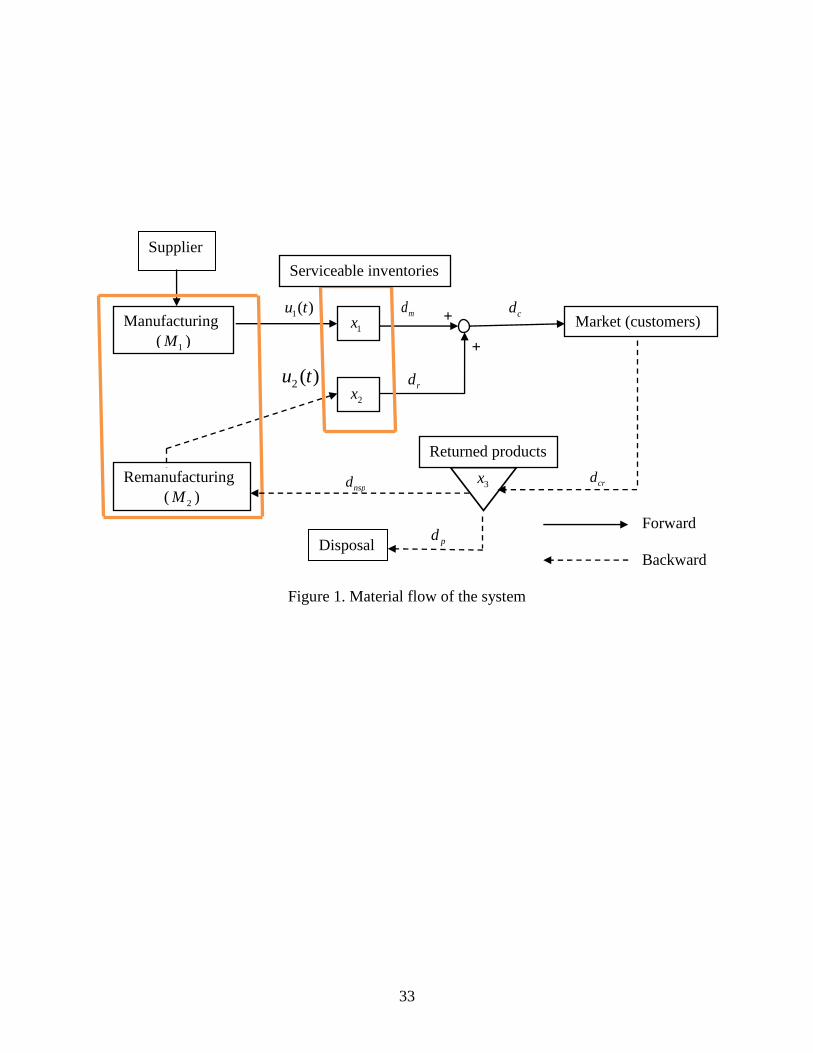
remanufacturing, respectively. We consider a one product recovery system where demands can

be fulfilled from an inventory for serviceable items. This inventory can be replenished by

production or by remanufacturing used and returned items. Another inventory is available for the

stock keeping of the returned items ahead of the remanufacturing process. Thus, returned items

can be remanufactured, disposed of, or be hold on stock for later remanufacturing. The situation

is illustrated in Figure 1.

The system behaviour is described by a hybrid state comprising both a continuous

component (stocks of products) and a discrete component (modes of the machines). The

continuous component consists of continuous variables 1 2( ), ( )x t x t and 3( )x t corresponding to

the stock level of manufactured products, remanufactured products and returned items.

These variables are described by three differential equations based on the dynamics of the

involved three stock levels illustrated in Figure 1.

12

1

2

3

11 1

22 2

33

( )( ) (0)

( )( ) (0)

( ) (0)

m

r

cr nsp p

dx tu t d x x

dt

dx tu t d x x

dt

dx td d d x x

dt

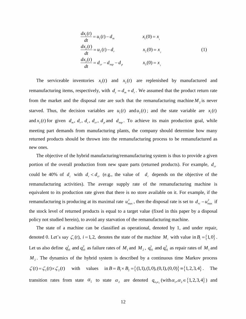
(1)

The serviceable inventories 1( )x t and 2 ( )x t are replenished by manufactured and

remanufacturing items, respectively, with c m rd d d . We assumed that the product return rate

from the market and the disposal rate are such that the remanufacturing machine 2M is never

starved. Thus, the decision variables are 1( )u t and 2 ( )u t ; and the state variable are 1( )x t

and 2 ( )x t for given , , , , m r c cr pd d d d d and nspd . To achieve its main production goal, while

meeting part demands from manufacturing plants, the company should determine how many

returned products should be thrown into the remanufacturing process to be remanufactured as

new ones.

The objective of the hybrid manufacturing/remanufacturing system is thus to provide a given

portion of the overall production from new spare parts (returned products). For example, crd

could be 40% of cd with r crd d (e.g., the value of rd depends on the objective of the

remanufacturing activities). The average supply rate of the remanufacturing machine is

equivalent to its production rate given that there is no store available on it. For example, if the

remanufacturing is producing at its maximal rate 2

maxu , then the disposal rate is set to 2

maxrcd u if

the stock level of returned products is equal to a target value (fixed in this paper by a disposal

policy not studied herein), to avoid any starvation of the remanufacturing machine.

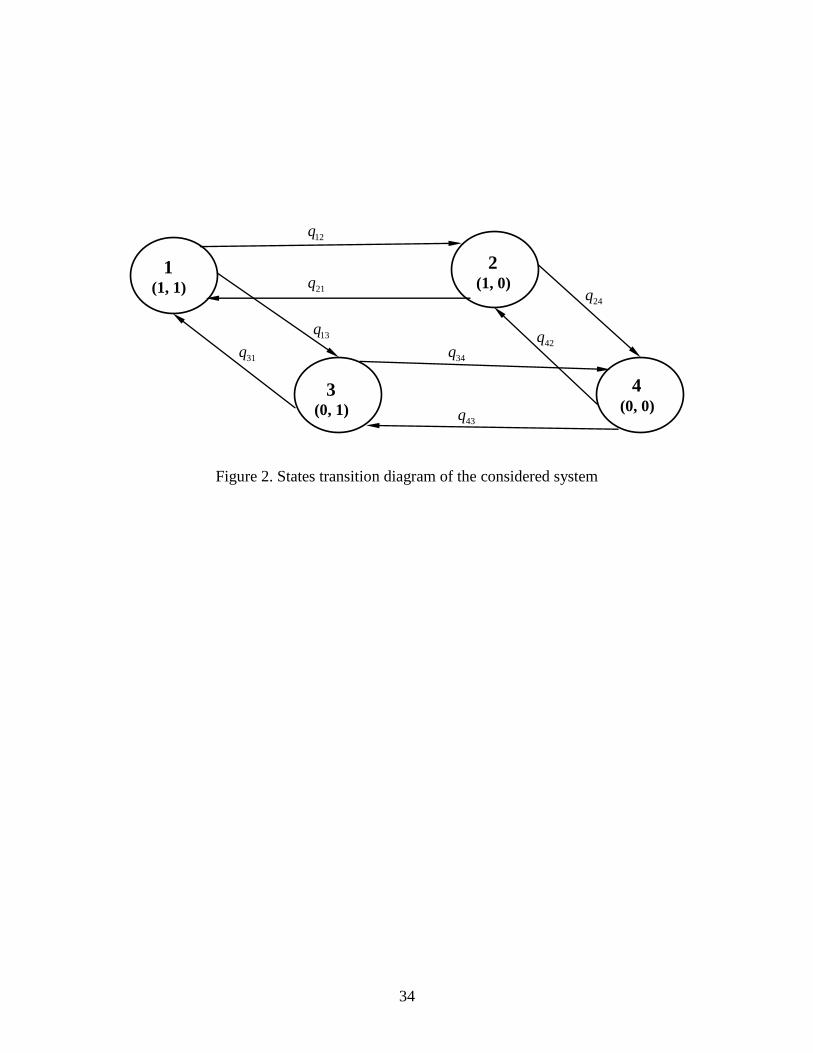
The state of a machine can be classified as operational, denoted by 1, and under repair,

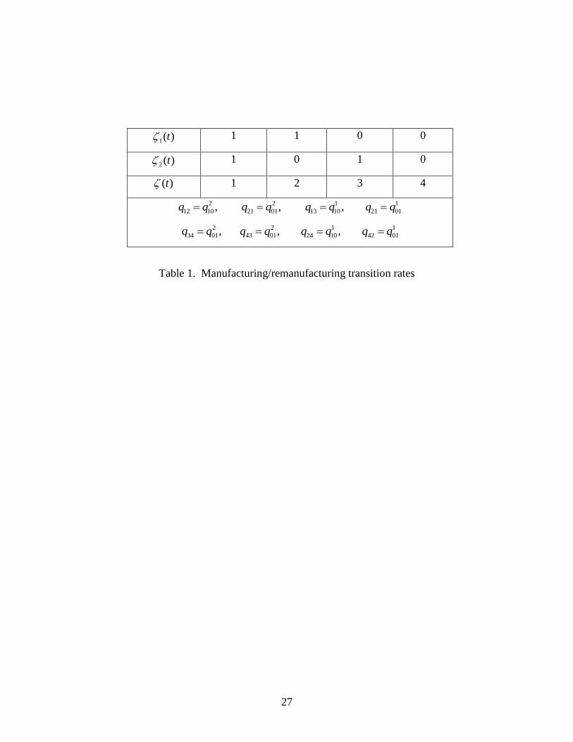
denoted 0. Let’s say ( ), 1,2,i t i denotes the state of the machine iM with value in 1,0iB .

Let us also define 1 2

10 10 and q q as failure rates of 1M and 2M , 1 2

01 01 and q q as repair rates of 1M and

2M . The dynamics of the hybrid system is described by a continuous time Markov process

1 2( ) ( ) ( )t t t with values in 1 2 (1,1),(1,0),(0,1),(0,0) 1,2,3,4B B B . The

transition rates from state 1 to state 2 are denoted 1 2

q (with 1 2, 1,2,3,4 ) and

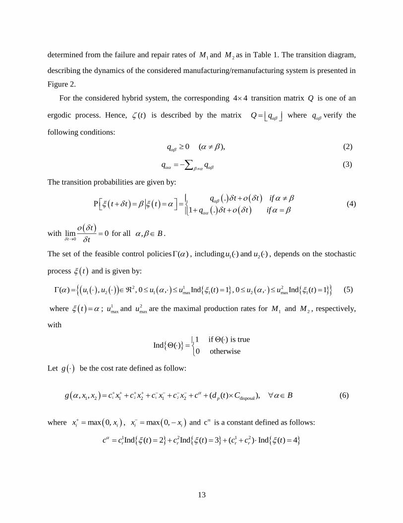
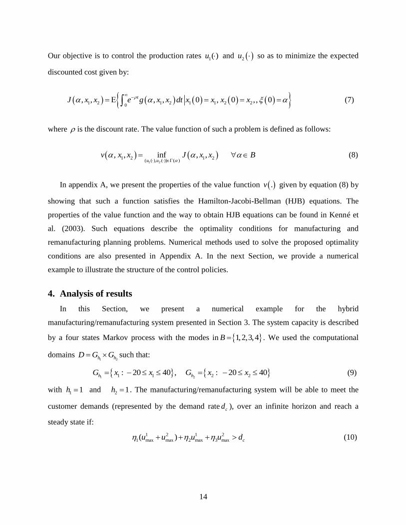
13

determined from the failure and repair rates of 1M and 2M as in Table 1. The transition diagram,

describing the dynamics of the considered manufacturing/remanufacturing system is presented in

Figure 2.

For the considered hybrid system, the corresponding 4 4 transition matrix Q is one of an

ergodic process. Hence, ( )t is described by the matrix Q q where q verify the

following conditions:

0 ( ),q (2)

q q (3)

The transition probabilities are given by:

.

1 .

q t t ift t t

q t t if

(4)

with

0lim 0t

t

t

for all , B .

The set of the feasible control policies ( ) , including 1 2( ) and ( )u u , depends on the stochastic

process t and is given by:

2 1 2

1 2 1 max 1 2 max 1( ) , , 0 , Ind ( ) 1 , 0 , Ind ( ) 1u u u u t u u t (5)

where t ; 1

maxu and 2

maxu are the maximal production rates for 1M and 2M , respectively,

with

1 if ( ) is true

Ind ( )0 otherwise

Let g be the cost rate defined as follow:

1 2 1 21 2 1 2 1 2 disposal, , ( ( ) ),pg x x c x c x c x c x c d t C B (6)

where max 0,i ix x , max 0,i ix x and c is a constant defined as follows:

1 2 1 2Ind ( ) 2 Ind ( ) 3 ( ) Ind ( ) 4r r r rc c t c t c c t

14

Our objective is to control the production rates 1( )u and 2u so as to minimize the expected

discounted cost given by:

1 2 1 2 1 1 2 20

, , , , 0 , 0 ,, 0tJ x x e g x x dt x x x x

(7)

where is the discount rate. The value function of such a problem is defined as follows:

1 2

1 2 1 2( ( ), ( )) ( )

, , inf , ,u u

v x x J x x B

(8)

In appendix A, we present the properties of the value function .v given by equation (8) by

showing that such a function satisfies the Hamilton-Jacobi-Bellman (HJB) equations. The

properties of the value function and the way to obtain HJB equations can be found in Kenné et

al. (2003). Such equations describe the optimality conditions for manufacturing and

remanufacturing planning problems. Numerical methods used to solve the proposed optimality

conditions are also presented in Appendix A. In the next Section, we provide a numerical

example to illustrate the structure of the control policies.

4. Analysis of results

In this Section, we present a numerical example for the hybrid

manufacturing/remanufacturing system presented in Section 3. The system capacity is described

by a four states Markov process with the modes in 1,2,3,4B . We used the computational

domains 1 2h hD G G such that:

1 21 1 2 2: 20 40 , : 20 40h hG x x G x x (9)

with 1 1h and 2 1h . The manufacturing/remanufacturing system will be able to meet the

customer demands (represented by the demand rate cd ), over an infinite horizon and reach a

steady state if:

1 2 1 2

1 max max 2 max 3 max( ) cu u u u d (10)

15

where , 1,2,3,k k is the limiting probability of the system at mode k . Note that the limiting

probabilities of modes 1, 2, 3 and 4 (i.e., 1 2 3 4, , and ), are computed as follows:

4

1

( ) 0 and 1i

i

Q

(11)

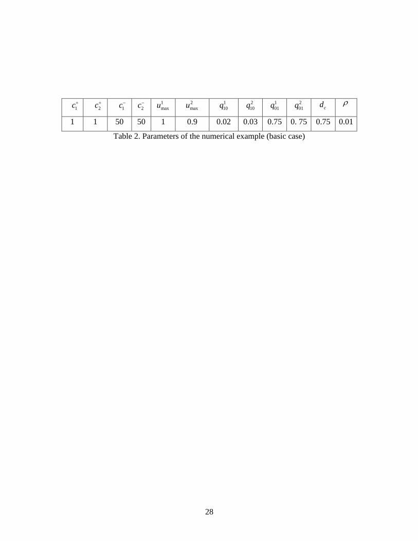
where 1 2 3 4( , , , ) ; and ( )Q is the corresponding 4 4 transition rate matrix. Table 2

summarizes the parameters used in this paper. The feasibility condition given by equation (11) is

satisfied for the chosen parameters if the raw material for the remanufacturing machine is always

available (as discussed previously). We obtain a 6.6% availability of the system (i.e., 6.6sAV ),

given by the following expression:

1 2 1 2

1 max max 2 max 3 max

100( )s c

c

AV u u u u dd

(12)

The policy improvement technique is used to solve the system of equations (A.4)-(A.7), see

appendix 1, for the data presented in table 2 with r c rd d R where rR is a return rate.

The first scenario investigated in this paper, for which the return rate (backward

direction) is defined as the quotient of the average returns R and the average demands of

serviceable products D (i.e., ` / /r R D r cR d d ) provides the manufacturing and

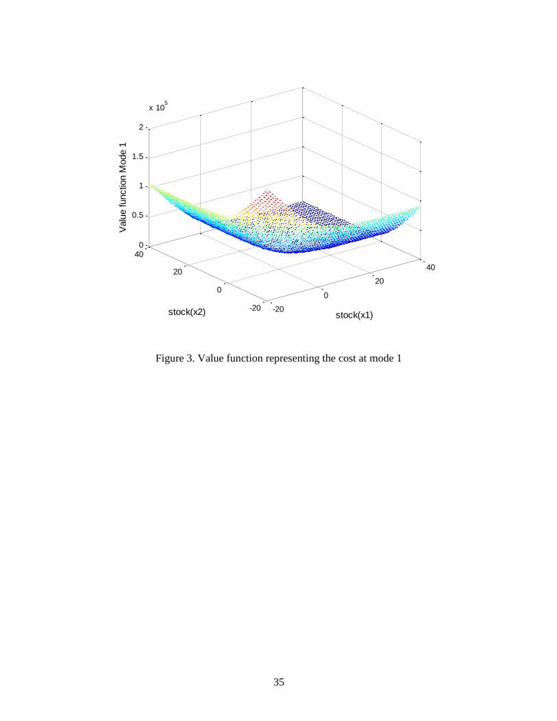
remanufacturing policies for 0.5r DR (i.e., 50%r cd d ). As a result, the value function

representing the cost and the production rates of manufacturing and remanufacturing machines

are obtained and depicted in Figures 3, 4a and 4b (for manufacturing), 5a and 5b (for

remanufacturing), respectively.

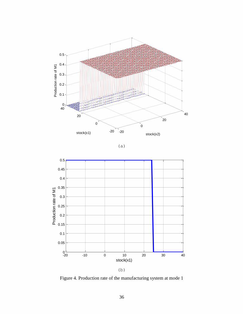
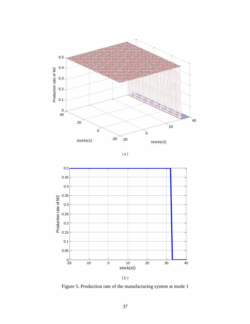
The production rates of the manufacturing and remanufacturing machines in their

operational mode (i.e., mode 1) are presented in Figures 4 and 5. The obtained manufacturing

and remanufacturing policies in modes 2 and 3 recommend to set the manufacturing rate (mode

2) or the remanufacturing rate (mode 3) to their maximal values given that the hybrid system is

feasible only at mode 1. There is no production in mode 4 given that both machines are down.

For the manufacturing policy, Figure 4 shows that there is no need to produce parts, using 1M

for comfortable stock levels. Then the production rate is set to zero when the stock level of

manufactured products is greater than 25 products as illustrated in figure 6. The structure of the

remanufacturing control policy is similar to the one of the manufacturing process with a different

16

threshold level. As illustrated in Figure 5, the production rate is set to zero when the stock level

of remanufacturing products is greater than 32 products. The threshold values of 25 and 32

products for manufacturing and remanufacturing are obtained from the numerical resolution of

equations (A.4) to (A.7) and well illustrated in Figures 4(b) and 5(b). The quantified feedback

policy obtained for this basic case and its implementation are illustrated in figure 6. Recall that,

in the considered forward-reverse logistics network, the remanufactured process brings returned

products back to as new condition. The bigger value of the remanufacturing threshold level,

compared to the manufacturing threshold level, is mainly due to the fact that the considered

mean time to failure of 1M is greater than the mean time to failure of 2M (i.e.,

1 2MTTF MTTFM M or 1 2

10 10q q ).

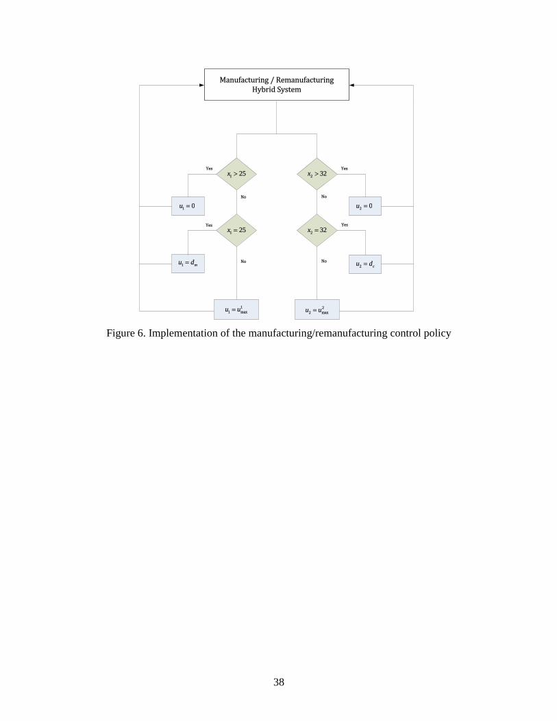
From the obtained results, and based on the illustration of Figure 6, the computational

domain is divided into three regions where the optimal production control policy consists of one

of the following rules:

1. Set the production rate of the manufacturing or remanufacturing system to its maximal

value when the current stock level is under the corresponding threshold value (1

Z for

manufacturing machine 1M and 2

Z for remanufacturing machine 2M ).

2. Set the production rate of 1M to the demand rate md when the current stock level of

manufactured products is equal to1

Z . Set also the production rate of 2M to the demand

rate rd when the current stock level of remanufactured products is equal to2

Z .

3. Set the production rates of manufacturing or remanufacturing machines to zero when

their current stock levels are larger than1 2

or Z Z .

The control policy obtained is an extension to the so-called hedging point policy given that

the previous three rules respect the structure presented in Akella and Kumar (1986). Thus, the

production policy for the manufacturing and remanufacturing at mode 1 are given

respectively by:

1 1

max 1 1

1

1 1 2 1 1

if ( )

( , ,1) if ( )

0 otherwise

c r

u x Z

u x x d d x Z

(13)

17

and

2 1

max 2 2

1

2 1 1 2 2

if ( )

( , ,1) if ( )

0 otherwise

r

u x Z

u x x d x Z

(14)

Using the control policies given by equations (13) and (14), the company will minimize the

total cost due to remanufacturing so that eventually it can maximise its total profit.

The previous results have been obtained for a return rate equal 50%. Let us first confirm the

structure of the control policies through a sensitivity analysis; and then observe the system for

different return rates. The aim of the sensitivity analysis is also to validate and illustrate the

usefulness of the model developed in this paper.

5. Sensitivity analysis

Sensitivity analyses are conducted on backlog cost parameters to gain insight into the

proposed stochastic model. The proposed model is also validated in this Section through a set of

experimental data reflecting practical industrial situation by considering a return rate different

from the one used in the previous Section. Extensions, based on some assumptions of the

developed mathematical model, are discussed in the next Section.

We performed a couple of experiments using the numerical example presented previously.

The results shown in Tables 3, 4, 5 and 6 represent two different situations in forward-reverse

logistics system analysis presented below for returned rates set to 50% and 25% respectively.

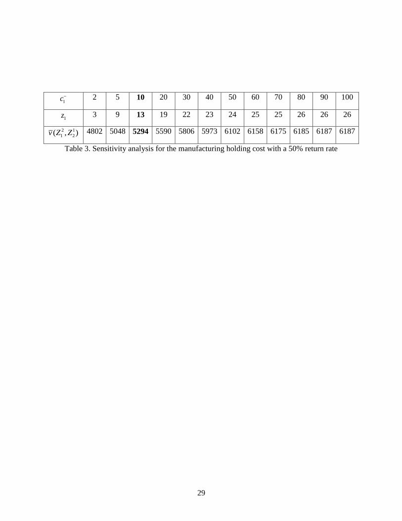
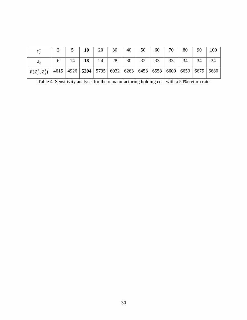
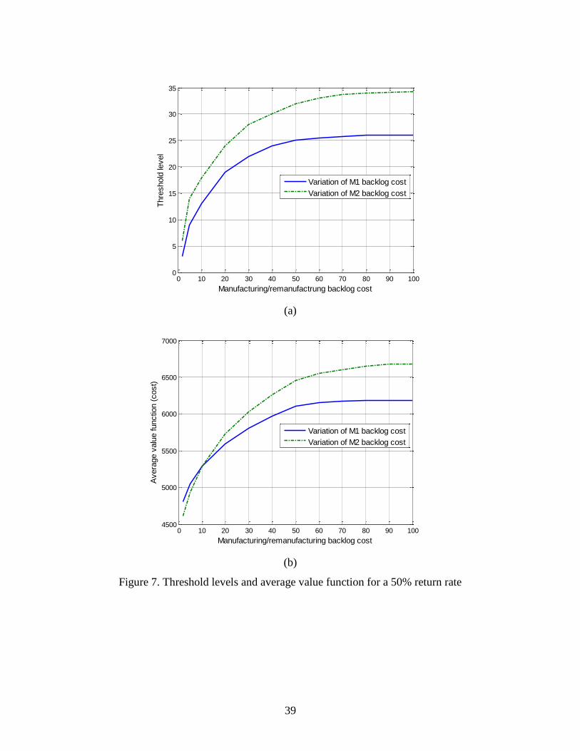
Figure 7, Tables 3 and 4 are based on the variation of manufacturing/remanufacturing backlog

costs for a 50% return rate.

The corresponding trend of variation for the threshold levels (manufacturing and

remanufacturing) and the incurred costs (represented by the average value function 2 1

1 2( , )v Z Z ) is

illustrated in Figure 7(a) and 7(b), respectively. One can observe that when the backlog costs

1 2 and c c increase, the threshold values 1 1

1 2 and Z Z also increase.

The overall cost also increases as well. In Tables 3 and 4, the experiment corresponding

to1 2

( , ) (10,10)c c , 2 1

1 2( , ) (13,18)Z Z and (13,18) 5294v is highlighted and is considered as a

basic case of the first block of backlog costs variations (i.e., for a return rate of 50%). The

parameters of the control policy move as predicted from a practical view point.

18

The sensitivity analysis performed in this paper, validates the proposed approach and shows

the usefulness of the proposed model given that the control policy is well defined by the

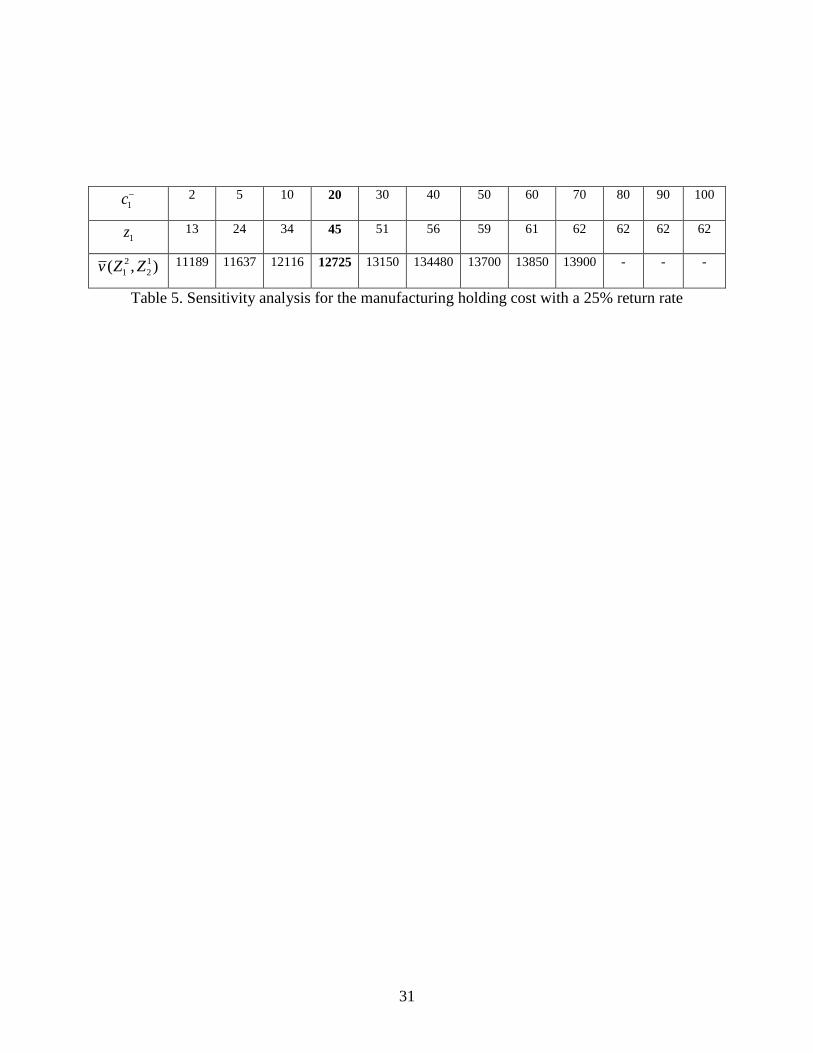
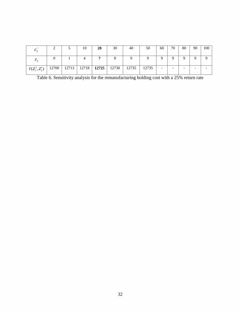
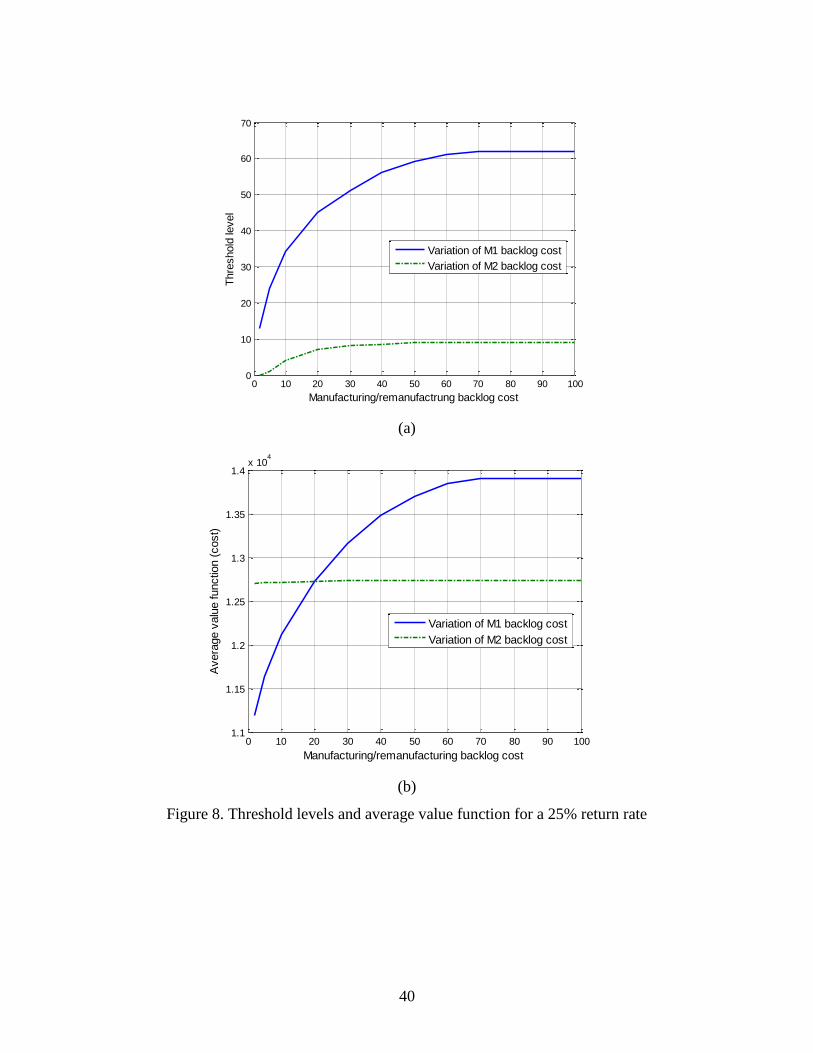
equations (13)-(14) and parameters obtained from results analysis. We also conducted a similar

sensitivity analysis for a return rate of 25% given that we assumed a known return rate instead of

trying to find it throw an optimization problem. Figure 7, Tables 5 and 6 are based on the

variation of manufacturing/remanufacturing backlog costs for a 25% return rate. As in the case

of 50% return rate, in Tables 5 and 6, the experiment corresponding to1 2

( , ) (20,20)c c ,

2 1

1 2( , ) (45,7)Z Z and (13,18) 12725v is highlighted and is considered as a basic case of the

second block of backlog costs variations (i.e., for a return rate of 25%).

The corresponding trend of variation for the threshold levels (manufacturing and

remanufacturing) and the incurred costs (represented by the average value function 2 1

1 2( , )v Z Z ) is

illustrated in Figure 8(a) and 8(b) respectively. When the backlog costs 1 2 and c c increase, the

threshold values 1 2 and z z also increase as in the case of 50% return rate. Due to the fact that the

return rate is 25%, the manufacturing and remanufacturing stock levels converge to 62 and 9

serviceable parts as their corresponding backlog cost is large.

The restriction that the remanufacturing process contributes just for 25% of the overall

production give a large threshold level for the 1M to ensure sufficient serviceable parts to hedge

against future failures of the machines.

6. Discussions and extensions

The proposed hybrid manufacturing/remanufacturing model can be applicable to the various

industries after specific customization. However, as the proposed model is introduced with

restrictive assumptions, many future works are accordingly needed. Above all, the proposed

model with backward information (remanufacturing) can be extended by adopting more industry

practices and so the relevant complex mathematical model need to be developed. Since the

proposed model is formulated as a markovian stochastic optimal model, the computational

burden for optimal solution increases exponentially as the size of problem increases (number of

machines, number of products, uncertainty on product demands and returns). Thus, in the future,

19

an efficient heuristic algorithm needs to be developed in order to solve the large-scale problems

in real industrial environment.

Recall that, for the system considered previously and related to a one manufacturing

machine, one remanufacturing machine and one-product, the control policy described by

equations (13) and (14) is completely known for given 1 2 and Z Z with 1,2,3 For a more

complex manufacturing system consisting of m machines for manufacturing, n machines

for remanufacturing, producing p different part types, the control policy depends on the

parameters kiZ , and kjZ , for 1,2 ,k p , 1,2 ,i m , 1,2 ,j n . The solution of the

HJB equations (as in equation (A.1)) is almost impossible for large , and m n p since the

dimension of the numerical scheme to be implemented increase exponentially with the

complexity of the system. Such a dimension is given by the following equation:

2

1 2

1 1

2 3 ( ) ( )p p

m n m n p

h j h j

j j

Dim N x N x

(15)

where ( ) card[ ( )]h kj h kjN x G x with 1k for manufacturing inventories and 2k for

remanufacturing inventories. The numerical grids for the manufacturing and remanufacturing

stock levels are 1( )h jG x and 2( )h jG x , respectively. Each machine has two modes (i.e.,

2m n modes for m n machines) and its production rate can take three values, namely maximal

production rate, demand rate and zero for manufactured and remanufactured products (i.e.,

23m n p possibilities for m -manufacturing machines, n -remanufacturing machines products an

p -products system). For example, in the case of 12 machines, 5 types of products

( 12, 5m n ), with 1 2( ) 100, ( ) 100h j h jN x N x , 1, ,5j , from equation (15), we have:

12 12 10 5 5 80Dim 2 3 100 100 7.36 10

The related numerical algorithm cannot be implemented on today computers. Such problems

are classified in the control literature as complex problems (Gershwin (1990)). For the

aforementioned complex problem (i.e., with , and m n p ), a hierarchical control approach as in

Kenné and Boukas (2003) or a combination of the control theory and the simulation based

experimental design as in Gharbi and Kenné (2003) can be used to obtain a near optimal control

policy. The use of simulation is more appropriate in this context because it provides a tool to

understand how the system behaves by carrying out «what-if» assessments and to identify which

20

factors are more important for further more detailed analysis (response surface analysis and

optimization). This could give the possibility to develop a more general model in reverse logistic

network including capacity limits, multi-product management and uncertainty on product

demands and returns.

7. Conclusion

The number of applications and scientific publications in the field of reverse logistics has

been steadily growing, reflecting the increasing importance of this subject, mainly as a result of

society’s accrued environment awareness and search for economic productivity. However, taking

a closer look to the dynamic characteristic of the production planning problems, one can notice

that reported work is mostly based on non machine-dynamic models and thus, general models

are missing, in particular models that relate reverse and forward chains. In this paper, the

production planning model of a hybrid manufacturing/remanufacturing system in reverse

logistics has been proposed in a continuous time stochastic context. We developed the stochastic

optimization model of the considered problem with two decision variables (production rates of

manufacturing and remanufacturing machines) and two state variables (stock levels of

manufactured and remanufactured products). By controlling both the manufacturing and

remanufacturing rates, we obtained a near optimal control policy of the system through

numerical techniques yielding straightforward decision rules. We illustrated and validated the

proposed approach using a numerical example and a sensitivity analysis. We finally discuss the

extension of the proposed model to the case of a forward-reverse logistics network involving

multiple products, multiple machines and uncertainty on product demands and returns.

Acknowledgements

The authors want to thank two anonymous referees whose critics and suggestions contributed

to significantly increase the quality of this paper.

21

Appendix A

Optimality conditions and numerical approach

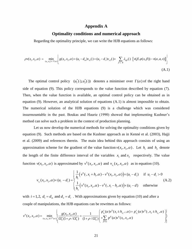
Regarding the optimality principle, we can write the HJB equations as follows:

1, 2

1 2 1 2 1 1 2 2( , ) ( )

( , , ) min ( , , ) ( ) ( ) ( ) ( ) ( ) ( , ( , )) ( , , )m x r xu u

B

v x x g x x u d v u d v v x v a x

(A.1)

The optimal control policy * *

1 2( ( ), ( ))u u denotes a minimiser over ( ) of the right hand

side of equation (9). This policy corresponds to the value function described by equation (7).

Then, when the value function is available, an optimal control policy can be obtained as in

equation (9). However, an analytical solution of equations (A.1) is almost impossible to obtain.

The numerical solution of the HJB equations (9) is a challenge which was considered

insurmountable in the past. Boukas and Haurie (1990) showed that implementing Kushner’s

method can solve such a problem in the context of production planning.

Let us now develop the numerical methods for solving the optimality conditions given by

equation (9). Such methods are based on the Kushner approach as in Kenné et al. (2003), Hajji

et al. (2009) and references therein. The main idea behind this approach consists of using an

approximation scheme for the gradient of the value function 1 2( , , )v x x . Let 1h and 2h denote

the length of the finite difference interval of the variables 1 2 and x x respectively. The value

function 1 2( , , )v x x is approximated by 1 2( , , )hv x x and 1 2( , , )ixv x x as in equation (10).

1 2

1 2

1 2

1( , , ) ( , , ) ( ) if 0

( , , ) ( )1

( , , ) ( , , ) ( ) otherwisei

h h

i i i i i i

i

x i i

h h

i i i

x

v x h v x x u d u dh

v x x u d

v x x v x h u dh

(A.2)

with 1 21,2, and m ri d d d d . With approximations given by equation (10) and after a

couple of manipulations, the HJB equations can be rewritten as follows:

1 1 2 2

1 2

1 21 2

1 2( , ) ( ) 1 2

( ) ( , , ) ( ) ( , , )( , , ) 1

( , , ) min( ) ( , , )(1 / ) (1 / )h

r

h h

x x x xh

hu u

h h h

p v x h p v x hg x x

v x xp v x x

22

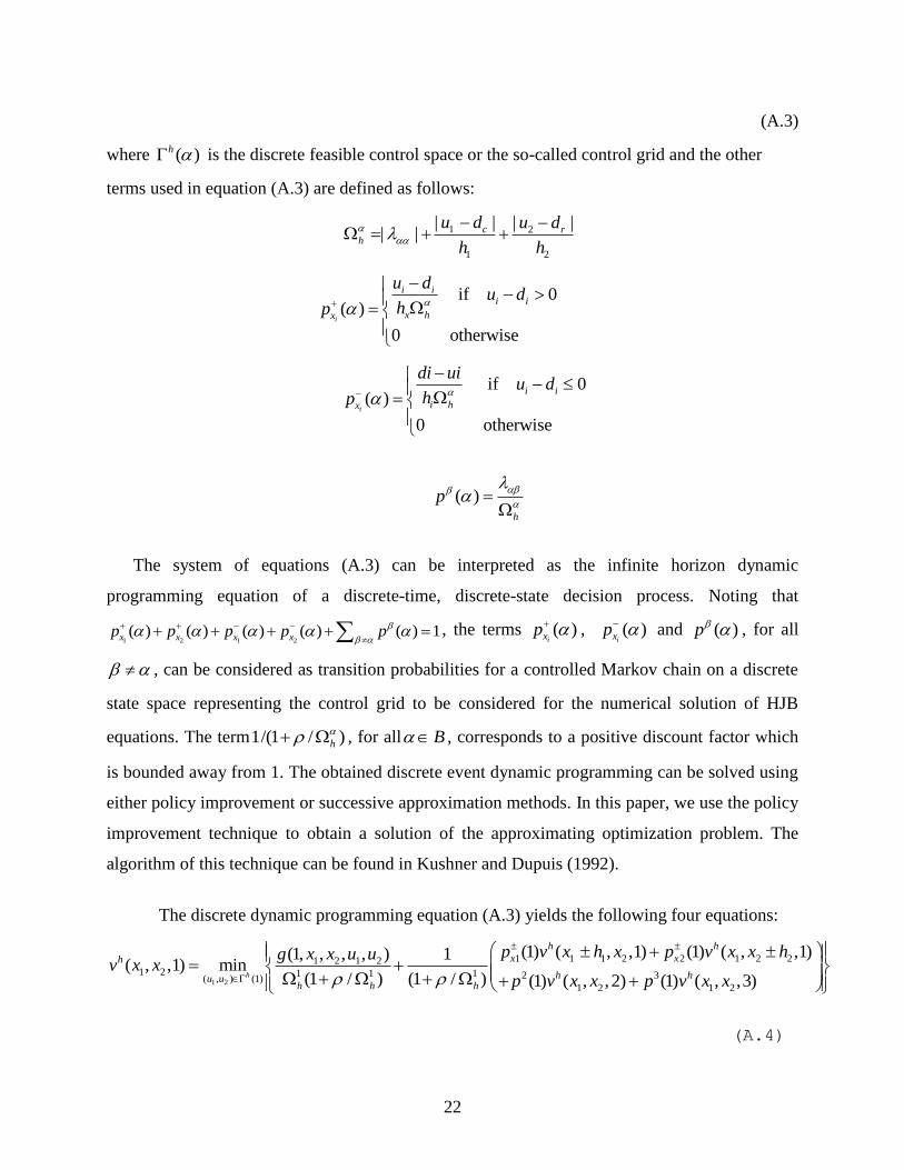
(A.3)

where ( )h is the discrete feasible control space or the so-called control grid and the other

terms used in equation (A.3) are defined as follows:

1 2

1 2

| | | || | c r

h

u d u d

h h

if 0 ( )

0 otherwisei

i ii i

x hx

u du d

hp

if 0

( )

0 otherwisei

i i

i hx

di uiu d

hp

( )h

p

The system of equations (A.3) can be interpreted as the infinite horizon dynamic

programming equation of a discrete-time, discrete-state decision process. Noting that

1 2 1 2( ) ( ) ( ) ( ) ( ) 1x x x xp p p p p

, the terms ( )

ixp , ( )ixp and ( )p , for all

, can be considered as transition probabilities for a controlled Markov chain on a discrete

state space representing the control grid to be considered for the numerical solution of HJB

equations. The term1/(1 / )h

, for all B , corresponds to a positive discount factor which

is bounded away from 1. The obtained discrete event dynamic programming can be solved using

either policy improvement or successive approximation methods. In this paper, we use the policy

improvement technique to obtain a solution of the approximating optimization problem. The

algorithm of this technique can be found in Kushner and Dupuis (1992).

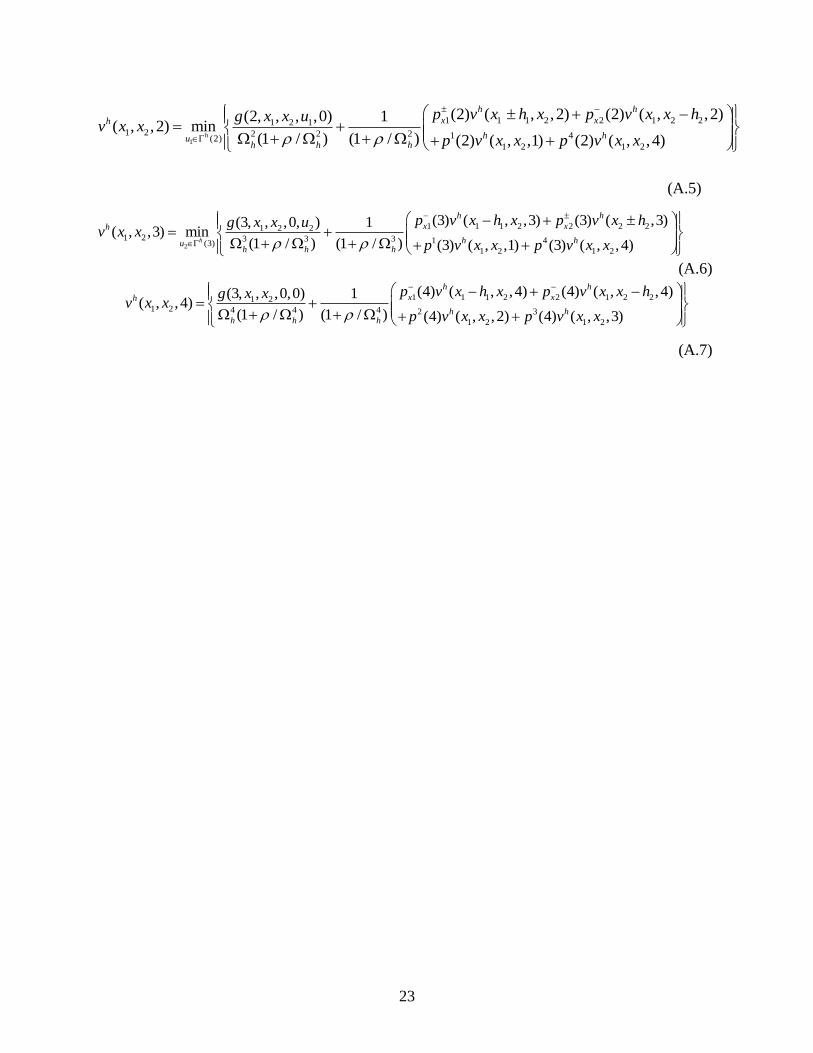
The discrete dynamic programming equation (A.3) yields the following four equations:

1 2

1 1 1 2 2 1 2 21 2 1 21 2 1 1 1 2 3( , ) (1)

1 2 1 2

(1) ( , ,1) (1) ( , ,1)(1, , , , ) 1( , ,1) min

(1 / ) (1 / ) (1) ( , ,2) (1) ( , ,3)h

h h

x xh

h hu uh h h

p v x h x p v x x hg x x u uv x x

p v x x p v x x

(A.4)

23

1

1 1 1 2 2 1 2 21 2 11 2 2 2 2 1 4(2)

1 2 1 2

(2) ( , ,2) (2) ( , ,2)(2, , , ,0) 1( , ,2) min

(1 / ) (1 / ) (2) ( , ,1) (2) ( , ,4)h

h h

x xh

h huh h h

p v x h x p v x x hg x x uv x x

p v x x p v x x

(A.5)

2

1 1 1 2 2 2 21 2 21 2 3 3 3 1 4(3)

1 2 1 2

(3) ( , ,3) (3) ( ,3)(3, , ,0, ) 1( , ,3) min

(1 / ) (1 / ) (3) ( , ,1) (3) ( , ,4)h

h h

x xh

h huh h h

p v x h x p v x hg x x uv x x

p v x x p v x x

(A.6)

1 1 1 2 2 1 2 21 21 2 4 4 4 2 3

1 2 1 2

(4) ( , ,4) (4) ( , ,4)(3, , ,0,0) 1( , ,4)

(1 / ) (1 / ) (4) ( , ,2) (4) ( , ,3)

h h

x xh

h hh h h

p v x h x p v x x hg x xv x x

p v x x p v x x

(A.7)

24

References

Akella, R., Kumar, P. R., Optimal Control of Production Rate in a Failure Prone

Manufacturing System, IEEE Trans. on Automatic Control, AC 31, 116-126, 1986

Amezquita, T. and Bras, B., Lean remanufacture of an Automobile Clutch, Proceedings of

First International Working Seminar on Reuse, Eindhoven, The Netherlands, p 6, 1996

Bostel, N., Dejax, P., Lu, Z., The Design, Planning and Optimization of Reverse Logistic

Networks, in Logistics Systems: Design and Optimization, A. Langevin, D. Riopel, editors,

Springer, 171-212, 2005

Boukas, E.K., Haurie, A., Manufacturing Flow Control and Preventive Maintenance: A

Stochastic Control Approach, IEEE Trans. on Automatic Control, 33, 1024-1031, 1990

Chung, S. L., Wee, H.M., Po-Chung, Y., Optimal Policy for a Closed-Loop Supply Chain

Inventory System With Remanufacturing, Mathematical and Computer Modelling, 6, 867-

881, 2008

Dobos, I., Optimal Production–Inventory Strategies for a HMMS-Type Reverse Logistics

System, International Journal of Production Economics, 81-82(11), 351-360, 2003

De Brito, M. P., Dekker, R., Flapper S. D. P., Reverse Logistics - a Review of Case Studies,

ERIM Report Series Reference No. ERS-2003-012-LIS, 2003

Dehayem, N.F.I., Kenné, J.P., Gharbi, A., Hierarchical Decision Making in Production and

Repair/Replacement Planning with Imperfect Repairs Under Uncertainties, European Journal

of Operational Research, 198( 1), 173-189, 2009

Dekker, R., Fleismann, M., Interfuth, K., Van Wassenhove L., edts., Reverse Logistics.

Quantitative models for closed-loops supply chains, 2004

Dong-Ping Song., Production and Preventive Maintenance Control in a Stochastic

Manufacturing System, International Journal of Production Economics, 19(1): 101-111, 2009

El-Sayed, M., Afia, N., El-Kharbotly, A., A Stochastic Model for Forward–Reverse Logistics

Network Design Under Risk, Computers & Industrial Engineering, In Press, 2008

Fleischmann, M., Bloemhof-Ruwaard, J.M., Dekker R., Van der, L.E., Van Nunen, J. A. E.

E., Van Wassenhove, L.N., Quantitative Models for Reverse Logistics: A review, European

Journal of Operational Research, 103(1), 1-17,1997

Gharbi, A., Kenné, J.P., Optimal Production Control Problem in Stochastic Multiple- Product

Multiple-Machine Manufacturing Systems, IIE transactions, 35, 941-952, 2003

Gharbi, A., Pellerin, R., Sadr, J., Production Rate Control for Stochastic Remanufacturing

Systems, International Journal of Production Economics, 112(1), 37-47, 2008

Gershwin, S. B., Manufacturing Systems Engineering, Prentice Hall, 1994

Geyer, R., Jackson, T., Supply Loops and Their Constraints: The Industrial Ecology of

Recycling and Reuse. California Management Review 46 (2), 55-73, Winter 2004.

25

Guide V.D.R. and Van Vassenhove, L.N., Closed-Loop Supply Chains, Feature Issue (Part

1), Production and Operations Management, Vol. 15, No 3, 2006

Guide V.D.R. and Van Vassenhove, L.N., Closed-Loop Supply Chains, Feature Issue (Part

2), Production and Operations Management, Vol. 15, No 4, 2006

Hajji, A., Gharbi, A., Kenné, J. P., Joint Replenishment and Manufacturing Activities

Control in Two Stages Unreliable Supply Chain, International Journal of Production

Research, 47(12), 3231-3251, 2009

Jorjani, S., Leu, J., Scott, C., Model for The Allocation of Electronics Components to Reuse

Options, International Journal of Production Research, 42(6), 1131-1145, 2004

Kenné, J.P., Boukas, E. K., Hierarchical Control of Production and Maintenance Rates in

Manufacturing Systems Journal of Quality in Maintenance Engineering, 9, 66-82, 2003

Kenné, J.P., Boukas, E.K., Gharbi, A., Control of Production and Corrective Maintenance

Rates in a Multiple-Machine, Multiple-Product Manufacturing System, Mathematical and

Computer Modelling, 38, 351-365, 2003

Kibum, K., Iksoo, S. Juyong, K., Bongju, J., Supply Planning Model for Remanufacturing

System in Reverse Logistics Environment, Computers & Industrial Engineering, 51( 2), 279-

287, 2006

Kiesmuller, G. P., Scherer, C. W., Computational Issues in a Stochastic Finite Horizon One

Product Recovery Inventory Model, European Journal of Operational Research, 146( 3), 553-

579, 2003

Kushner, H.J., Dupuis, J., Numerical Methods for Stohastic Control Problems in Continuous

Time, Springer-Verlag, 1992

Lund, R., The Remanufacturing Industry: Hidden Giant, Boston, Massachusetts: Boston

University, 1996

Ostlin, J., Sundin, E., Bjorkman, M., Importance of Closed-Loop Supply Chain Relationships

for Product Remanufacturing, International Journal of Production Economics, Volume 115,

336-348, 2008

Pellerin, R., Sadr, J., Gharbi, A., Malhamé ,R., A Production Rate Control Policy for

Stochastic Repair and Remanufacturing Systems, International Journal of Production

Economics, In Press, 2009

Rishel, R., Dynamic Programming and Minimum Principles for Systems With Jump Markov

Disturbances, SIAM journal on Control, 13, 338-371, 1975

Rogers, D. S., Tibben-Lembke, R.S., Going backwards: reverse logistics trends and

practices, Center for Logistics Management, University of Nevada, Reno, Reverse Logistics

Executive Council, 1998

Salema, M. I. G., Barbosa-Povoa, Ana Paula, Novais, A. Q., An Optimization Model for the

Design of a Capacitated Multi-Product Reverse Logistics Network With Uncertainty,

European Journal of Operational Research, 179(3), 1063-1077, 2007

26

Seaver, W.B., Design Considerations for Remanufacturability, Recyclability and Reusability

and Reusability of User Interface Modules, Proceedings of IEEE International Symposium

on Electronics and the Environment, (IEEE-94), San Francisco, CA, USA, 241-245, 1994

Seierstad, A., Sydsaeter, K., Optimal Control Theory with Economic Applications. North-

Holland, Amsterdam, 1987

Sundin, E. and Bras B., Making Functional Sales Environmentally and Economically

Beneficial through Product Remanufacturing. Journal of Cleaner Production, Vol. 13(9), pp

913-925, 2005

Thierry, M.C., M. Salomon, M., Van Nunen, J., Van Wassenhove, L., Strategic Issues in

Product Recovery Management, California Management Review 37, 114-135, 1995

Verter, V., Boyaci, T., edts, Special issue on Reverse Logistics, Computers and Operations

Research, 34, 295-298.

27

1( )t 1 1 0 0

2 ( )t 1 0 1 0

( )t 1 2 3 4

2 2 1 1

12 10 21 01 13 10 21 01, , , q q q q q q q q

2 2 1 1

34 01 43 01 24 10 42 01, , , q q q q q q q q

Table 1. Manufacturing/remanufacturing transition rates

28

1c 2c 1c 2c 1

maxu 2

maxu 1

10q 2

10q 1

01q 2

01q cd

1 1 50 50 1 0.9 0.02 0.03 0.75 0. 75 0.75 0.01

Table 2. Parameters of the numerical example (basic case)

29

1c 2 5 10 20 30 40 50 60 70 80 90 100

1z 3 9 13 19 22 23 24 25 25 26 26 26

2 1

1 2( , )v Z Z 4802 5048 5294 5590 5806 5973 6102 6158 6175 6185 6187 6187

Table 3. Sensitivity analysis for the manufacturing holding cost with a 50% return rate

30

2c 2 5 10 20 30 40 50 60 70 80 90 100

2z 6 14 18 24 28 30 32 33 33 34 34 34

2 1

1 2( , )v Z Z 4615 4926 5294 5735 6032 6263 6453 6553 6600 6650 6675 6680

Table 4. Sensitivity analysis for the remanufacturing holding cost with a 50% return rate

31

1c 2 5 10 20 30 40 50 60 70 80 90 100

1z 13 24 34 45 51 56 59 61 62 62 62 62

2 1

1 2( , )v Z Z 11189 11637 12116 12725 13150 134480 13700 13850 13900 - - -

Table 5. Sensitivity analysis for the manufacturing holding cost with a 25% return rate

32

2c 2 5 10 20 30 40 50 60 70 80 90 100

2z 0 1 4 7 8 9 9 9 9 9 9 9

2 1

1 2( , )v Z Z 12700 12713 12718 12725 12730 12735 12735 - - - - -

Table 6. Sensitivity analysis for the remanufacturing holding cost with a 25% return rate

33

md

2 ( )u t

nspd

Figure 1. Material flow of the system

Manufacturing

( 1M )

Remanufacturing

( 2M )

Market (customers)

Disposal

Supplier

1x

X1

2x

X2

Forward

Backward

1( )u t

cd

rd

pd

crd 3x

Returned products

(customers)

+

+

Serviceable inventories

ories(customers)

34

Figure 2. States transition diagram of the considered system

1 (1, 1)

2 (1, 0)

3 (0, 1)

4 (0, 0)

12q

21q

24q

42q

43q

34q

13q

31q

35

-20

0

20

40

-20

0

20

400

0.5

1

1.5

2

x 105

stock(x1)stock(x2)

Valu

e functio

n M

ode 1

Figure 3. Value function representing the cost at mode 1

36

-20

0

20

40

-20

0

20

400

0.1

0.2

0.3

0.4

0.5

stock(x2)stock(x1)

Pro

duction r

ate

of

M1

(a)

-20 -10 0 10 20 30 400

0.05

0.1

0.15

0.2

0.25

0.3

0.35

0.4

0.45

0.5

stock(x1)

Pro

ductio

n r

ate

of M

1

(b)

Figure 4. Production rate of the manufacturing system at mode 1

37

-20

0

20

40

-20

0

20

400

0.1

0.2

0.3

0.4

0.5

stock(x2)stock(x1)

Pro

duction r

ate

of

M2

(a)

-20 -10 0 10 20 30 400

0.05

0.1

0.15

0.2

0.25

0.3

0.35

0.4

0.45

0.5

stock(x2)

Pro

ductio

n r

ate

of M

2

(b)

Figure 5. Production rate of the manufacturing system at mode 1

38

Manufacturing / RemanufacturingHybrid System

No No

No No

Yes Yes

YesYes

1 25x 2 32x

1 25x 2 32x

1 0u 2 0u

1 mu d2 cu d

1

1 maxu u 2

2 maxu u

Figure 6. Implementation of the manufacturing/remanufacturing control policy

39

0 10 20 30 40 50 60 70 80 90 1000

5

10

15

20

25

30

35

Manufacturing/remanufactrung backlog cost

Thre

shold

level

Variation of M1 backlog cost

Variation of M2 backlog cost

(a)

0 10 20 30 40 50 60 70 80 90 1004500

5000

5500

6000

6500

7000

Manufacturing/remanufacturing backlog cost

Avera

ge v

alu

e functio

n (

cost)

Variation of M1 backlog cost

Variation of M2 backlog cost

(b)

Figure 7. Threshold levels and average value function for a 50% return rate

40

0 10 20 30 40 50 60 70 80 90 1000

10

20

30

40

50

60

70

Manufacturing/remanufactrung backlog cost

Thre

shold

level

Variation of M1 backlog cost

Variation of M2 backlog cost

(a)

0 10 20 30 40 50 60 70 80 90 1001.1

1.15

1.2

1.25

1.3

1.35

1.4x 10

4

Manufacturing/remanufacturing backlog cost

Avera

ge v

alu

e functio

n (

cost)

Variation of M1 backlog cost

Variation of M2 backlog cost

(b)

Figure 8. Threshold levels and average value function for a 25% return rate