Jean Morlet and the Continuous Wavelet Transform · Morlet and the Continuous Wavelet Transform...

Morlet and the Continuous Wavelet Transform

CREWES Research Report — Volume 28 (2016) 1

Jean Morlet and the Continuous Wavelet Transform

Brian Russell1 and Jiajun Han1

1 Hampson-Russell, A CGG GeoSoftware Company, Calgary, Alberta, [email protected]

ABSTRACT Jean Morlet was a French geophysicist who used an intuitive approach, based on

his knowledge of seismic processing algorithms, to propose a new method of time-frequency analysis. Geophysicists did not at first recognize the originality of Morlet’s work, but mathematicians did, and his method was re-named the Continuous Wavelet Transform, or CWT, and lead to a new branch of mathematics. In this article, we will re-visit Morlet’s classic papers and show why his work was so original and important. we will also show a modern application of the CWT to seismic data analysis.

INTRODUCTION

Jean Morlet was a geophysicist who worked for Total in France. In 1982 he and three co-authors published two papers in Geophysics (Morlet et al., 1982 I and II) proposing a new approach to time-frequency analysis (Cohen, 1995) based on wavelets. The key ideas that make Morlet’s work so original were as follows:

1. First, he used the Gabor wavelet, a sinusoidally-modulated Gaussian function,as his wavelet of choice.

2. Second, he used the Heisenberg uncertainty principle to keep the product ofthe time and frequency widths of the wavelets constant.

3. Third, he defined the width of the of the wavelet envelope as an integer timesthe dominant period of the sinusoid, introducing a shape factor.

4. Fourth, he used a logarithmic increment in the frequency domain, introducingwhat now is called scale.

5. Finally, he cross-correlated each of his wavelets with the input seismic trace toanalyze the frequency content of the trace.

In the following discussion, we will derive Morlet’s approach by analyzing each of the above steps, then descibe the modern formulation of the CWT and its applications to seismic data analysis. But we will start by going further back to the work of Dennis Gabor on communication theory that was the inspiration for Morlet’s work (Gabor, 1946). This seminal paper has inspired much of the research in time-frequency analysis since its publication (e.g., see Cohen, 1995).

GABOR’S ELEMENTARY SIGNAL

Before summarizing the work of Morlet et al. (1982 I and II) it is instructive to go back and look at the pioneering work of Gabor (1946), which was the starting point for Morlet’s work. Russell (2013) discusses the impact of Gabor’s work on modern seismic data analysis.

mailto:[email protected]

Russell and Han

2 CREWES Research Report — Volume 28 (2016)

Dennis Gabor was a quantum physicist who turned his attention to information theory. He is most famous for winning the 1971 Nobel Prize in Physics for his invention holography. Gabor (1946) applied Heisenburg’s uncertainty principle to the time-frequency Fourier pair to define what he called his “elementary signal”. Recall that the uncertainty principle in quantum mechanics is written as

2

≥∆∆ px , (1)

where ∆x is uncertainty in position, ∆p is uncertainty in momentum and π2h

= is

Planck’s constant divided by 2π. That is, the product of the uncertainties in position and momentum can never get below the value 2/ . In a similar way for time signals, Gabor (1946) proposed that the product of the uncertainty in the time signal and the frequency signal can never get below one-half, which can be written

21

≥∆∆ ft , (2)

where ∆t is uncertainty in time, ∆f is uncertainty in frequency. Gabor then designed an “elementary signal” for which the product given in equation 2 is exactly equal to one-half. Gabor (1946) writes the time domain signal as

[ ] ( )φπαψ +−−= tfittt 02

02 2exp)(exp)( , (3)

where α defines the sharpness of the pulse, t0 its centre, f0 its dominant frequency, φ its initial phase and ( ) ( ) ( )φπφπφπ +++=+ tfitftfi 000 2cos2cos2exp , where 1−=i . Note that this is the same formulation as the “wave packet” used by quantum physicists (McWeeny, 1972).

Gabor (1946) then computed the Fourier transform of the signal in equation (3), finding it to be

( )φπαπφ +−−

−

−= )(2exp)(exp)( 00

20

2

fftifff , (4)

To make sure that the product in equation (2) is equal to 1/2, Gabor (1946)

setsα

π 12

=∆t andπ

α2

=∆f . He also defines the term α as the bandwidth f2-f1 of the

ideal band-pass filter defined by

12

1sin)(ffffkf

−−

= πφ , (5)

where f2 and f1 are the cutoff points of the filter. Equations (3) and (4) define what we would now call a Gabor wavelet, in time and frequency respectively.



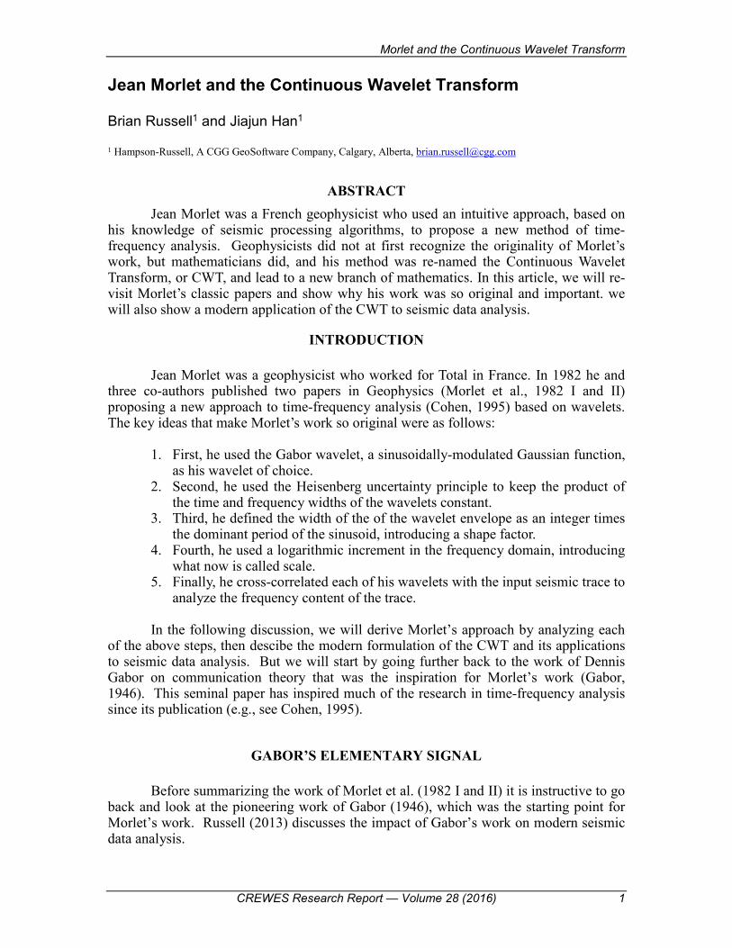
Figure 1, from Gabor (1946), shows the envelopes of the time and frequency signals defined in equations (3) and (4).

Figure 1: The envelopes of the time and frequency forms of the Gabor wavelets given in equations (3) and (4) (from Gabor, 1946).

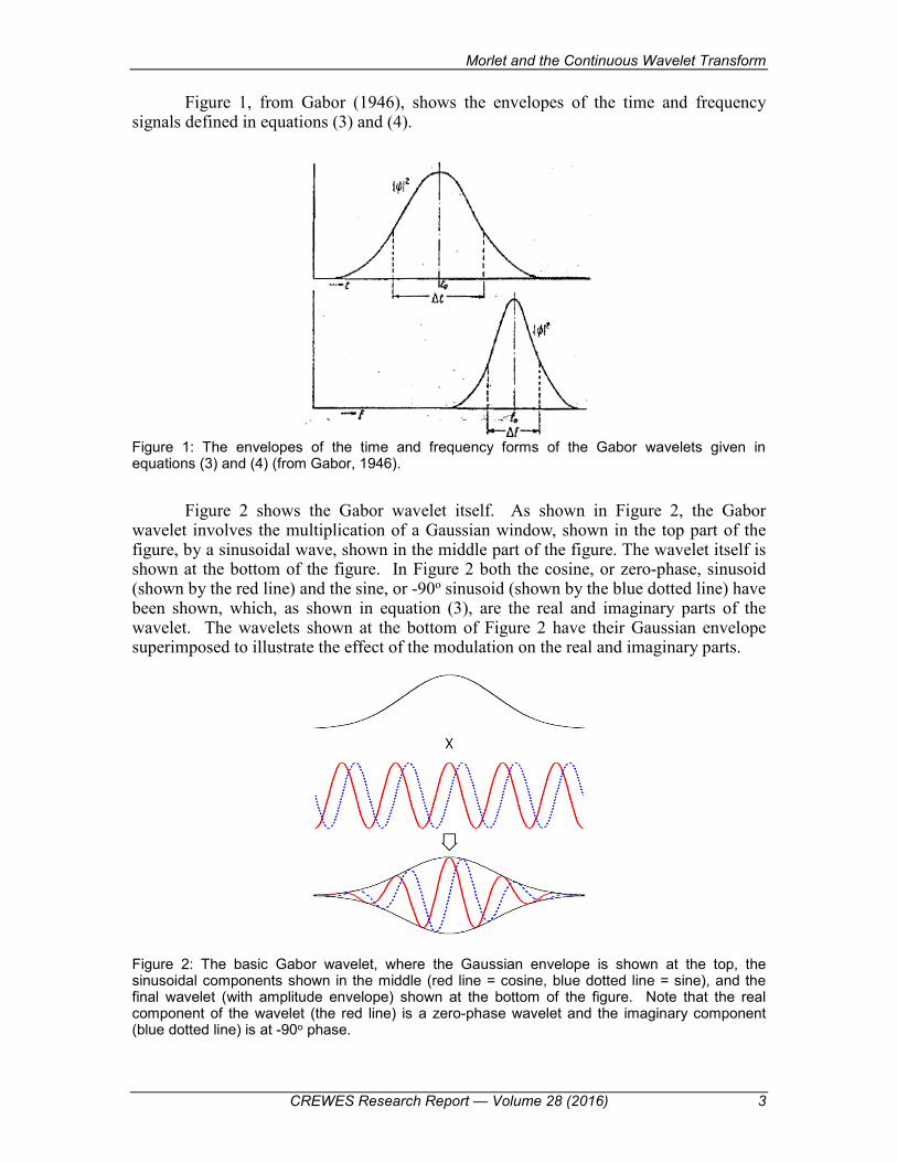
Figure 2 shows the Gabor wavelet itself. As shown in Figure 2, the Gabor wavelet involves the multiplication of a Gaussian window, shown in the top part of the figure, by a sinusoidal wave, shown in the middle part of the figure. The wavelet itself is shown at the bottom of the figure. In Figure 2 both the cosine, or zero-phase, sinusoid (shown by the red line) and the sine, or -90o sinusoid (shown by the blue dotted line) have been shown, which, as shown in equation (3), are the real and imaginary parts of the wavelet. The wavelets shown at the bottom of Figure 2 have their Gaussian envelope superimposed to illustrate the effect of the modulation on the real and imaginary parts.

Figure 2: The basic Gabor wavelet, where the Gaussian envelope is shown at the top, the sinusoidal components shown in the middle (red line = cosine, blue dotted line = sine), and the final wavelet (with amplitude envelope) shown at the bottom of the figure. Note that the real component of the wavelet (the red line) is a zero-phase wavelet and the imaginary component (blue dotted line) is at -90o phase.

Russell and Han


MORLET’S EXTENSION OF GABOR’S WORK

Let us next see how Morlet re-expressed the Gabor wavelet and extended the concept to create the continuous wavelet transform, or CWT. Referring back to equation (3) and Figure 2, note that the Gabor wavelet can be expressed as

)()()( tstgt =ψ , (6)

where g(t) is the Gaussian window and s(t) is the sinusoidal component. If we assume that the phase component of equation (3) is equal to zero, we can express the sinusoidal component as

( ) ,sincosexp)( 000 tittits ωωω +== (7)

where period. mean andfrequency mean , 22 ,1 000

00 ====−= TfT

fi ππω Figure 3

shows a sinusoid with period T0, where the cosine function starts on a peak (or zero

phase) and the sine function is a -90o phase shifted cosine.

Figure 3: A pure sinusoid function, with period T0.(red line = cosine, blue dots = sine).

Note that the theoretical sinusoid shown in Figure 3 is infinite in extent. Thus, the effect of a Gaussian window is to restrict the sinusoid to a reasonable length.

Next, let us consider the Gaussian envelope function, as shown in Figure 4.

Morlet et al. (1982, II) rewrote the Gabor version of the wavelet that was shown in equation (3) as

,2ln2exp)(2

∆−=

tttg (8)

where envelope. Gaussian of width andfrequency angular mean 0 =∆= tω

Thus, instead of defining t∆

=1

2πα , as Gabor (1946) does, Morlet et al. (1982, II)

define the width as t∆

=2ln2α . The reason for this change in the definition of α is best



seen in Figure 4. Referring to Figure 4, if we define the time width of the Gabor wavelet as the difference between the two times at which the envelope is one-half its maximum amplitude, note that by substituting into equation 8 we get

[ ] 5.02lnexp)()( 11 =−=−= tgtg .

Figure 4: The time domain Gaussian envelope function, which reaches half its maximum at ∆t.

The complete Gabor wavelet, as shown earlier in Figure 3, can thus be written as the product of equations 7 and 8, or

( )tit

tt 0

2

exp2ln2exp)( ωψ

∆−= . (9)

Morlet et al. (1982, II) then compute the Fourier transform of the Gabor wavelet

and showed that it is equal to:

−∆

−∆=Ψ2

0

2ln4)(exp

2ln21)( ωωπω tt . (10)

As seen in Figure 5, we can next define a the angular frequency width ∆ω as the difference between the angular frequency values of the Fourier transform of the wavelet reach an amplitude of on-half of the maximum, or the angular frequencies given by

2/01 ωωω ∆−= and 2/02 ωωω ∆+= .

Figure 5: The frequency domain Gaussian envelope function reaches one-half of its maximum symmetrically around ω0 at a width of ∆ω.

Russell and Han


From Figure 5, we can therefore compute the equivalent Heisenberg uncertainty

rule for the Morlet et al. (1982, II) version of the Gabor (1946) wavelet. First, we set the ratio of the spectra from equation (10) at either ω1 and ω0 or ω2 and ω0 to 1/2, or

( )

( )( )

21

2ln64exp

0exp2ln64

exp

)()(

)()( 2

2

0

2

0

1 =

∆∆−=

∆∆−

=ΨΨ

=ΨΨ ω

ω

ωω

ωω t

t

.

Next, taking logarithms we get

2ln64)(2ln

2ω∆∆=

t .

Simplifying, this gives the angular frequency x time width as

2ln8=∆∆ tω ,

or the frequency x time width as

883.02

2ln8≈=∆∆

πtf . (11)

Note that this value is slightly larger than Gabor’s value of 0.5.

Figure 6, taken from Morlet et al. (1982, Part II), shows a representative wavelet and its Fourier transform, where the time and frequency widths have been annotated. Note that we could have called this a Gabor wavelet, but since Morlet’s conventions have been used in building this wavelet, we will call it a Morlet wavelet. This nomenclature will be even more convincing when we introduce the concept of the “shape ratio” in the next paragraph.

Figure 6: A representative Morlet wavelet Fourier pair (from Morlet et al., 1982, part II).



Another way in which Morlet et al. (1982, Part II) differ from Gabor (1946) is that they define the time width of the wavelet as a function of the dominant period (or dominant frequency) rather than the frequency bandwidth. This is done by defining a “shape ratio” k, which relates the Gaussian time width at half-amplitude to the mean period using the equation

∆t = kT0. (12) Note that this also means, from equation (11), that the frequency width is given by

kf

kTkTf 0

00

883.0883.02

2ln8=≈=∆

π.

Referring back to Figure 6 (and Figure 3) note that k = 2 in this example. Since

T0 = 0.02 sec, this means that ∆t = 0.04 sec, f0 = 50 Hz and ∆f = 22 Hz, as shown in the figure.

Figure 7 shows the effect of three different shape ratios (1, 2 and 4) for a constant

dominant period of T0 = 20 ms. Notice that higher shape ratios have more side lobes. In modern applications of the CWT, the shape ratio appears to be fixed at a value of 2, but from Figure 7 it would appear that there are advantages to being able to change the shape ratio.

Figure 7: The effect of different values of k on the shape of the Morlet wavelet.

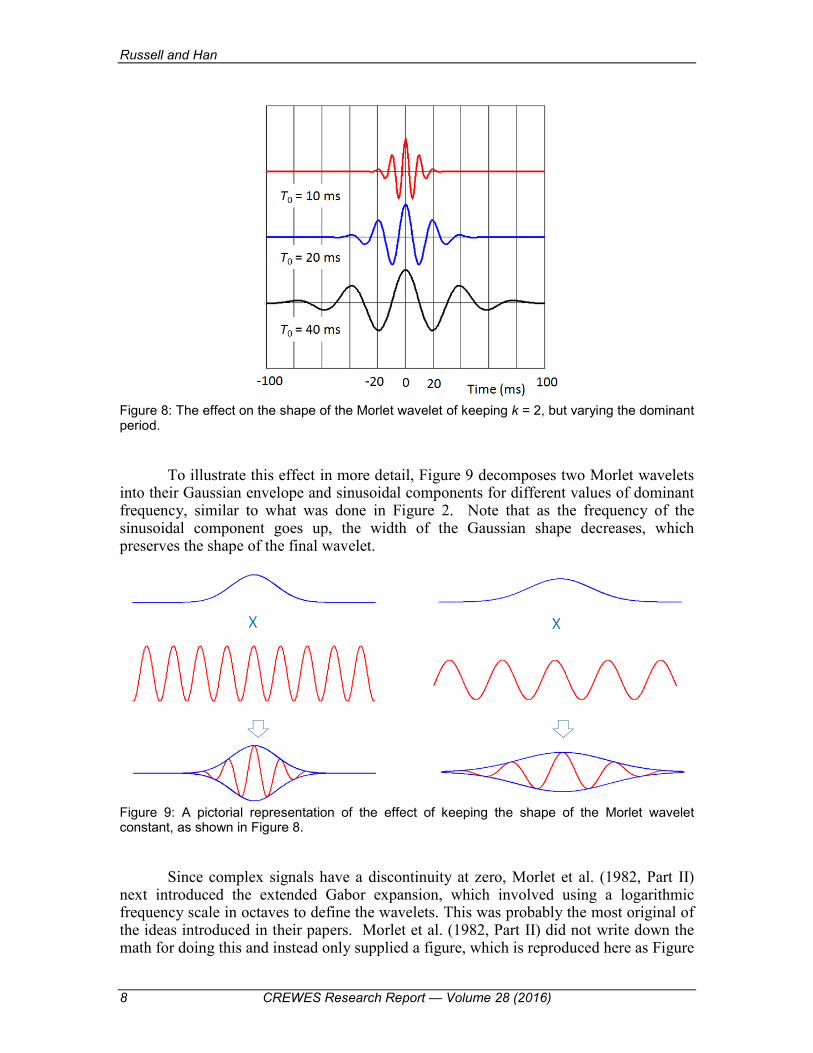
Next, let us look at the effect of keeping the shape ratio fixed and varying the

dominant period of the Morlet wavelet. This is shown in Figure 8, where we have used dominant periods of 10, 20 and 40 ms (equivalent to dominant frequencies of 100, 50 and 40 Hz, respectively, or Gaussian time widths of 20, 40 and 80 ms, respectively). Note that this has the interesting effect of stretching while preserving shape as the stretching proceeds.

Russell and Han


Figure 8: The effect on the shape of the Morlet wavelet of keeping k = 2, but varying the dominant period.

To illustrate this effect in more detail, Figure 9 decomposes two Morlet wavelets

into their Gaussian envelope and sinusoidal components for different values of dominant frequency, similar to what was done in Figure 2. Note that as the frequency of the sinusoidal component goes up, the width of the Gaussian shape decreases, which preserves the shape of the final wavelet.

Figure 9: A pictorial representation of the effect of keeping the shape of the Morlet wavelet constant, as shown in Figure 8.

Since complex signals have a discontinuity at zero, Morlet et al. (1982, Part II)

next introduced the extended Gabor expansion, which involved using a logarithmic frequency scale in octaves to define the wavelets. This was probably the most original of the ideas introduced in their papers. Morlet et al. (1982, Part II) did not write down the math for doing this and instead only supplied a figure, which is reproduced here as Figure



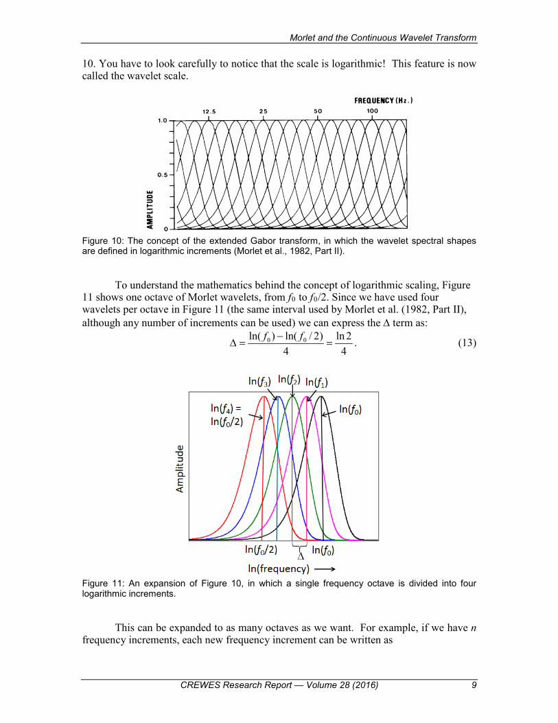
10. You have to look carefully to notice that the scale is logarithmic! This feature is nowcalled the wavelet scale.

Figure 10: The concept of the extended Gabor transform, in which the wavelet spectral shapes are defined in logarithmic increments (Morlet et al., 1982, Part II).

To understand the mathematics behind the concept of logarithmic scaling, Figure 11 shows one octave of Morlet wavelets, from f0 to f0/2. Since we have used four wavelets per octave in Figure 11 (the same interval used by Morlet et al. (1982, Part II), although any number of increments can be used) we can express the ∆ term as:

42ln

4)2/ln()ln( 00 =

−=∆

ff . (13)

Figure 11: An expansion of Figure 10, in which a single frequency octave is divided into four logarithmic increments.

This can be expanded to as many octaves as we want. For example, if we have n frequency increments, each new frequency increment can be written as

Russell and Han


2ln)4/()ln()ln( 0 nffn −= . (14)

Equation 14 can also be expressed as:

( ) ( ) 4/0

0 22ln)4/(exp)ln(exp nn

fnff =⋅= . (15)

Equation 15 has therefore introduced the scale parameter for four steps per

octave, s = 2n/4, but this can be generalized to s = 2n/m, where n is the number of steps below the starting frequency and m is the number of wavelets per octave. Using the scale parameter s and the shape parameter k allows us to re-write both the time and frequency forms of the wavelet using only one other parameter, the dominant frequency ω0. The time domain form is given as

−= t

si

sktskt 0

20 exp2lnexp),,( ωπ

ωψ , (16)

and the frequency domain form is

−−

=Ψ

2

00

12ln2

1exp2ln

),,(ωπω

ωππω sksksk . (17)

Now we get to the final step, which involves cross-correlating each wavelet ψt

with the seismic trace st to obtain its wavelet transform. Recall that the discrete correlation formula is given as follows where, since we are dealing with a complex wavelet, we must first take the complex conjugate of the wavelet (indicated by the asterisk on ψk*):

),1(,),1(,)(1

0

* −−−== ∑−

=− NMsc

N

kkks τψτ τψ (18)

where ( ) ( ).,,, and ,,,,, 1102/02/ −− == MtNNt ssss ψψψψ

A faster approach is to apply frequency domain correlation. In the frequency domain, correlation involves multiplication of the complex conjugate of the frequency domain wavelet with the Fourier transform of the seismic signal, or

)()()( * ωωω SCGS Ψ= , (19) where [ ]tsFS =)(ω and F is the forward Fourier transform. To obtain the time domain cross-correlation, we simply apply the inverse Fourier transform to the frequency domain cross-correlation:



[ ])()( 1 ωτψ Ss CFc Ψ−= , (20)

where ransform. Fourier tinverse theis 1−F This is the procedure used in the implementation of the CWT in the final example in this paper.

THE MODERN FORMULATION OF THE CWT

The modern mathematical formulation of the continuous wavelet transform (e.g. Daubechies, 1992) is written:

,)(1),( *∫∞

∞−

−

= dta

ttsa

aSWτψτ (21)

.03.1 and , where 00 == aaa m The term a is the scale, and ψ(t) is called the “mother” wavelet, defined by:

( ) ( ),2/2/4/1 200

2 ωωπψ −−−− −= eeet tit (22)

.2ln

2 where 0 =ω

Although the concept of scale has been preserved in the above formulation, and the method has been improved by the addition of an overall scaling term, the concept of shape has been lost as well as any physical intuition about the process. This is the forumulation which we will use in the next two examples, one a synthetic and one a real data example. However, as stated earlier, the correlation will be done in the frequency domain.

SYNTHETIC EXAMPLE

Figure 12 shows a synthetic trace consisting of a 20Hz cosine wave, a 100Hz Morlet atom at 0.3 s, two 30Hz Ricker wavelets at 1.1 s and three other frequency components.

Russell and Han


Figure 12: A synthetic trace consisting of a 20Hz cosine wave, a 100Hz Morlet atom at 0.3 s, two 30Hz Ricker wavelets at 1.1 s and three other frequency components (Han and van der Baan, 2013).

Figure 13 shows the amplitude spectrum of the synthetic trace, where the individual components cannot be discerned.

Figure 13: The amplitude spectrum of the synthetic trace of the trace shown in Figure 12.

Figure 14(a) shows The application of the short-time Fourier transform, with a 170 ms sliding window. Because of the fixed time-frequency resolution of this STFT, it can’t distinguish between the two Ricker wavelets.

Time

Freq

uenc

y

Short time Fourier transform

0.5 1 1.5 2

0

20

40

60

80

100

120

140

160

180

200

1

2

3

4

5

6

7

8

9

(a) (b)



Figure 14: The application of the (a) short-time Fourier transform with a 170 ms sliding window, and (b) the CWT, using a starting frequency of 200 Hz and 325 scales (Han and van der Baan, 2013)..

In Figure 14(b), we apply the CWT, using a starting frequency of 200 Hz and 325

scales. Note the better separation of the components and frequency resolution. In the next, and final, section we will apply the STFT and CWT to a real data example from Alberta.

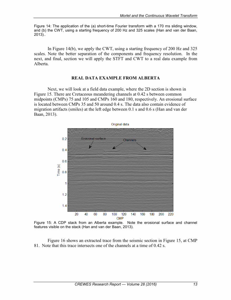
REAL DATA EXAMPLE FROM ALBERTA

Next, we will look at a field data example, where the 2D section is shown in Figure 15. There are Cretaceous meandering channels at 0.42 s between common midpoints (CMPs) 75 and 105 and CMPs 160 and 180, respectively. An erosional surface is located between CMPs 35 and 50 around 0.4 s. The data also contain evidence of migration artifacts (smiles) at the left edge between 0.1 s and 0.6 s (Han and van der Baan, 2013).

Figure 15: A CDP stack from an Alberta example. Note the erosional surface and channel features visible on the stack (Han and van der Baan, 2013).

Figure 16 shows an extracted trace from the seismic section in Figure 15, at CMP

81. Note that this trace intersects one of the channels at a time of 0.42 s.

Russell and Han


Figure 16: An extracted trace from the seismic section in Figure 15, at CMP 81, which intersects one of the channels at a time of 0.42 s (Han and van der Baan, 2013).

Figure 17(a) shows the application of the short time Fourier transform (STFT) to CMP 81 from Figure 16. Figure 17(b) shows the application of the continuous wavelet transform (CWT) to CMP 81 from Figure 16. Note the improvement in resolution on the CWT, especially at the channel event at 0.42 s.

(a) (b)

Figure 17: The application of: (a) the short time Fourier transform, or STFT, and (b) the continuous wavelet transform, CWT, to CMP 81, as shown in Figure 16 (Han and van der Baan).

The STFT of the complete seismic section from Figure 15 is shown in Figure 18(a). The CWT of the complete seismic section from Figure 15 is shown in Figure 18(b). The colour scales are given in Hz. Again, note the improvement in resolution of the channels on the CWT over the STFT.



Figure 18: The application of: (a) the STFT (Han and van der Baan) and (b) the CWT (Herrera et al., 2014) to the complete seismic section shown in Figure 15. The colour scales are in Hz.

CONCLUSIONS

In this report, we have shown how Morlet formulated a new approach to seismic frequency analysis in his classic 1982 papers. Morlet took a number of concepts that were familiar to geophysicists at the time, such as wavelets, the Fourier transform, logarithmic bandwidth and cross-correlation, and put them together in a totally new way. His conceptual approach was then formalized by mathematicians into a comprehensive new theory called the continuous wavelet transform, or CWT. Although the new theory was much more complete than Morlet’s original theory, it was also much less rooted in physical intuition.

In the last two sections of the report, we applied the CWT to both a synthetic dataset and a seismic section recorded in Alberta, and compared the results to the short time Fourier transform, or STFT. In both cases the resolution improvement of the CWT over the STFT was apparent.

REFERENCES

Cohen, L., 1995, Time-Frequency Analysis: Prentice-Hall PTR. Daubechies, I, 1992, Ten Lectures on Wavelets: SIAM, CBMS-NSF Regional Conference Series in

Applied Mathematics. Gabor, D., 1946, Theory of communication, part I: J. Int. EE., 93, part III, p. 429-441. Han, J. and van der Baan, M., 2013, Empirical mode decomposition for seismic time-frequency analysis:

Geophysics, 78, O9-O19. Herrera, R.H., Han, J. and van der Baan, M, 2014, Applications of the synchrosqueezing transform in

seismic time-frequency analysis: Geophysics, 79, V55-V64. McWeeny, R., 1972, Quantum Mechanics: Principles and Formalism: Dover Publications, Inc., Mineola,

New York. Morlet, J., Arens, G., Fourgeau, E., and Giard, D., 1982a, Wave propagation and sampling theory – Part I:

Complex signal and scattering in multilayered media: Geophysics, 47, p. 203-221. Morlet, J., Arens, G., Fourgeau, E., and Giard, D., 1982b, Wave propagation and sampling theory – Part II:

Sampling theory and complex waves: Geophysics, 47, p. 222-236. Russell, B., 2013, Dennis Gabor: The father of seismic attribute analysis: Canadian Journal of Exploration

Geophysics, 38, 22-31.

ACKNOWLEDGEMENTS We want to thank our colleagues at the CREWES Project and at CGG and Hampson-

Russell for their support and ideas, as well as the sponsors of the CREWES Project.

Jean Morlet and the Continuous Wavelet Transform · Morlet and the Continuous Wavelet Transform...

Documents

Transcript of Jean Morlet and the Continuous Wavelet Transform · Morlet and the Continuous Wavelet Transform...