Learning by Doing vs. Learning from Others in a Principal-Agent

Model∗

Jasmina Arifovic† Alexander Karaivanov‡

October, 2009

Abstract

We introduce learning in a principal-agent model of stochastic output sharing under moral haz-ard. Without knowing the agents’ preferences and the production technology, the principal triesto learn the optimal agency contract. We implement two learning paradigms — social (learningfrom others) and individual (learning by doing). We use a social evolutionary learning algorithm(SEL) to represent social learning. Within the individual learning paradigm, we investigate theperformance of reinforcement learning (RL), experience-weighted attraction learning (EWA), andindividual evolutionary learning (IEL). Our results show that learning in the principal-agent modelis very difficult due to three main reasons: (1) the stochastic environment, (2) the discontinuity inthe payoff space at the optimal contract caused by the binding participation constraint and (3) theincorrect evaluation of foregone payoffs in our sequential game principal-agent setting. The firsttwo factors apply to all learning algorithms we study while the third is the main reason for EWA’sand IEL’s failures to adapt. We find that social learning, especially with a selective replicationoperator, is much more successful in adapting to the optimal contract than the canonical versionsof individual learning from the literature. A modified version of the IEL algorithm using realizedpayoffs evaluation performs better than the other individual learning models; however, it still fallsshort of the social learning’s performance.

Keywords: learning, principal-agent model, moral hazard

JEL Classifications: D83, C63, D86

∗We thank Nick Kasimatis, Sultan Orazbayev and Sophie Wang for excellent research assistance. We also thank GeoffDunbar, Ken Kasa and participants at the Society of Economic Dynamics and the Computing in Economics and Financeconferences for their useful comments and suggestions. Both authors acknowledge the support of the Social Sciences andHumanities Research Council of Canada.

†Department of Economics, Simon Fraser University, 8888 University Drive, Burnaby, BC, V5A 1S6, Canada; email:arifovic@sfu.ca

‡Department of Economics, Simon Fraser University, 8888 University Drive, Burnaby, BC, V5A 1S6, Canada; email:akaraiva@sfu.ca

1

1 Introduction

The optimal contracts in principal-agent models often take complicated forms, for example, due to theintricate trade-off between provision of insurance and incentives. Depending on the exact setting, theoptimal contract depends crucially on both the principal’s and agent’s preferences, the properties ofthe production technology, and the stochastic properties of the income process. As an example, takea standard problem of optimal contracting under moral hazard (e.g. Hart and Holmstrom, 1987)1.The existing literature typically assumes that actions undertaken by the agent are unobservable ornon-verifiable by the principal. However, at the same time, the principal is assumed to have perfectknowledge of objects that seem much harder or at least as hard to know or observe such as the agent’spreferences, the agent’s decision making process, or the functional form of the output technology.

In this paper, we address these issues by explicitly modeling the principal’s learning process basedonly on observables such as output realizations. Our primary objective is to investigate whether thislearning process leads to knowledge acquisition sufficient for convergence to the theoretically optimalprincipal-agent contract. To this end we analyze two alternative paradigms, social and individuallearning, to describe the principal’s learning process. The social learning paradigm represents a wayof explicit, micro-level modeling of what is referred to in the literature as “learning spillovers”, or“learning from others”. At the same time, the individual learning paradigm can be viewed as anexplicit, micro-level modeling of “learning by doing” (e.g. Arrow, 1962; Stokey, 1988).

Numerous empirical studies in widely diverse research areas suggest that individuals and firmsutilize in practice social and individual learning methods resembling those we analyze. For example, inindustrial organization, Thornton and Thompson (2001) use a dataset on shipbuilding during WWIIto analyze learning across and within shipyards. They find that learning spillovers are significant andmay have contributed more to increases in productivity than conventional learning by doing effects.Cunningham (2004) uses data from semiconductor plants and finds that firms which are installingsignificantly new technologies appear to be influenced by social learning. Singh, Youn and Tan (2006)find similar effects in the open source software industry. In the development literature, Foster andRosenzweig (1996) use household panel data from India on the adoption and profitability of high-yield crop varieties to test the implications of learning by doing and learning from others. They findevidence that both households’ own and their neighbors’ experience increase profitability. Conley andUdry (2005) investigate the role of social learning in the diffusion of a new agricultural technology inGhana2. They test whether farmers adjust their inputs to align with those of their neighbors whowere successful in previous periods and present evidence that farmers do tend to adopt such successfulpractices. However, when they apply the same model to a crop with a known technology they findno such effect3. Last but not least, at the macro level, the seminal works of Romer (1986) and Lucas(1988) have emphasized the role of learning spillovers as an engine of economic growth.

Specifically, we adopt a repeated one-period contracting framework in an output-sharing modelwhich can be thought of as optimal wage, sharecropping, or equity financing arrangement. An assetowner (the principal) contracts with an agent to produce jointly. The principal supplies the asset(e.g. a machine, land, know-how, etc.) while the agent supplies unobservable labor effort. Output is

1Applications that fit under this heading abound in the finance literature (credit under moral hazard), public finance(optimal taxation with hidden labor effort), development (sharecropping), macroeconomics (optimal social insurance),labor (optimal wage schedules), etc.

2See also Zhang et al. (2002) who present evidence for learning from others in technology adoption in India.3Further evidence exists in the business / management literature. For instance, Boyd and Bresser (2004) study the

occurrence and performance impact of different models of organizational learning in the U.S. retail industry and pointout the importance of inter-organizational learning, while Ryu, Rao, Kim and Chaudhury (2005) document learning bydoing and learning from others in the Internet data management sector.

2

stochastic and the probability of a given output realization depends on the agent’s effort. The principalwants to design and implement an optimal compensation scheme for the agent which maximizes theprincipal’s profits and satisfies participation and incentive compatibility constraints.

We first describe the optimal contract that arises if both contracting parties are fully rational andknow all the ingredients of the contracting problem and environment. Then, we model and analyze thesituation in which a principal (or, principals) with no prior knowledge of the environment has to learnwhat the optimal contract is.

We implement the social learning paradigm (learning from others) via a model of social evolutionarylearning, SEL, in which players update their strategies based on imitating strategies of those playerswho have performed better in the past, and, occasionally, experimenting with new strategies. Thepopulation of players thus learns jointly through their experience that they share over time4. Toimplement the individual learning paradigm (learning by doing), we evaluate three algorithms thathave been widely used in various game theoretic and applied settings: reinforcement learning, RL(Roth and Erev, 1995, 1998), experience-weighted attraction learning, EWA (Camerer and Ho, 1999)5,and individual evolutionary learning, IEL (Arifovic and Ledyard, 2004, 2007). In contrast to sociallearning, individual learning is based on updating the entire collection of strategies that belong to anindividual player, based on her own experience only.

Two features shared by all the algorithms are the increase in frequency of representation of well-performing strategies over time and the probabilistic choice of a particular strategy to be used in agiven period. In terms of payoff evaluation, the difference between RL on one hand, and IEL andEWA, on the other, is that RL updates the payoff only of the strategy that was played in a giventime period, and leaves the payoffs of the rest of the strategies unchanged. In contrast, EWA and IELconstantly update the payoffs of all strategies based on their ‘foregone’ payoffs. In terms of strategyrepresentation, what distinguishes RL and EWA from IEL is that the implementation of RL and EWArequires representation of all possible strategies set in the algorithms’ strategy collections, while IELstarts out with a collection (i.e. a subset) of strategies that are randomly drawn from the full set.Finally, in terms of payoff updating, RL and EWA use a procedure that is standard for a number ofindividual learning algorithms, i.e. the probabilities that strategies will be selected are updated basedon their accumulated payoffs while IEL’s updating is instead based on the evolutionary paradigm, i.e.,consists of increases in frequency of the strategies that performed well in the past (based on evaluationof their foregone payoffs) and occasional experimentation with new strategies6

Our results show that social evolutionary learning almost always converges to the theoreticallyoptimal principal-agent contract. In contrast, the individual learning algorithms based on evaluationof foregone payoffs (IEL and EWA) that have proven very successful in a variety of Nash environmentscompletely fail to adapt in our setting. Reinforcement learning (RL) performs somewhat better than

4Our implementation of the evolutionary paradigm is based on genetic algorithms which have had numerous appli-cations in economics — for example, Arifovic (1996), Arifovic (2000), Marks (1998), Dawid (1999), Lux and Schorstein(2005). Also, in organization theory, Rose and Willemain (1996) implement a genetic algorithm in a principal-agentenvironment where the principal’s and agent’s strategies are represented by finite automata. They find that the varianceof output and agent’s risk aversion affect adaptation. However, they do not analyze the relative performance of differentlearning algorithms nor study the reasons for non-convergence.

5For an excellent overview of applications of RL, EWA and other individual learning models see Camerer (2003) andErev and Haruvy (2008).

6Arifovic (1994) implemented IEL in the context of the ‘cobweb’ model and showed it captured well price behavior inexperiments with human subjects. More recently, Hommes and Lux (2008) use an individual genetic algorithm to matchexperimental data about expectations in cobweb settings. Our IEL implementation follows Arifovic and Ledyard (2004)who apply it to public good provision mechanisms and call market mechanisms to capture, in real time, behavior observedin experiments with human subjects. Overall, IEL has proven to be especially successful in adapting to environmentswith large strategy spaces (e.g., see Arifovic and Ledyard, 2004 for comparison with RL and EWA).

3

IEL and EWA since it only updates the payoffs of those strategies that were actually used. However,RL’s overall learning performance is also unsatisfactory relative to SEL’s due to RL’s disadvantage inhandling the large strategy space.

The intuition for the failure of EWA and IEL is that, when evaluating foregone payoffs of potentialstrategies that have not been tried out, the principal assumes that agent’s action will remain con-stant (as if playing Nash), while in fact the optimal contract involves a reaction to the agent’s bestresponse function as in a Stackelberg game. The inability of these canonical individual learning modelsto produce correct foregone payoffs for the principal’s strategies precludes their convergence to thetheoretically optimal contract7. In contrast, social learning involves evaluation of payoffs of only thosestrategies that are actually played, thus avoiding this problem. As a result, SEL exhibits high rates ofconvergence to the optimal contract.

Two additional reasons, specific to the principal-agent setting, cause further difficulties with adapt-ing to the optimal contract, independently of the learning algorithm used. First, as usual, the presenceof stochastic shocks makes learning difficult in any type of environment. Second, in ours and anysimilar mechanism design model, the principal’s payoffs are a discontinuous function of the strategyspace at the agent’s participation constraint. That is, profits are maximized at some positive valueat a point on the constraint but any nearby contract which violates it yields zero payoff that in turnresults in a large flat area in the payoff function. This creates problems for the successful adaptationof all learning algorithms since their performance is driven by the differences in payoffs that strategiesreceive over time.

The failure of individual learning where foregone payoffs are taken into account stands in starkcontrast to the findings reported in the existing literature. However, our principal-agent environmentis different from the environments studied so far, most importantly in its sequential as opposed tosimultaneous game nature. To address this problem, we evaluate a modified version of the IEL algorithmwhere only payoffs of strategies that are actually tried out are updated while, at the same time,we keep the evolutionary updating mechanism that allows IEL to adapt well in environments withlarge strategy space as reported in the literature. The resulting ‘IEL with realized payoffs’ (IELR)algorithm does much better in adapting to the optimal contract than its canonical ‘foregone payoffs’counterpart. Nevertheless, the IELR’s convergence rates still fall short of those achieved with sociallearning, including when controlling for the total number of strategies being evaluated over a simulationrun. 8

2 Contracting with Full Rationality

Consider a standard moral hazard model of output/equity sharing, for example, Stiglitz (1974) onsharecropping in agriculture. Other applications include profit sharing under franchising, licensing, orauthor-publishing contracts. To fix ideas, interpret the principal as the owner of a productive asset

7Note that another commonly studied learning algorithm, fictitious play (Fudenberg and Levine, 1998) would sufferfrom the same problem in our setting, as it also uses foregone payoffs.

8Comparative studies of social and individual evolutionary learning have been done before in the context of the‘cobweb’ model, e.g. Arifovic (1994), Vriend (2000), and Arifovic and Maschek (2006). Arifovic (1994) shows that bothsocial and individual evolutionary learning converge to the Walrasian equilibrium. Her individual learning algorithm usesevaluation of hypothetical payoffs. On the other hand, Vriend (2000) demonstrates that while social learning convergesto the Walrasian equilibrium, individual learning reaches the Cournot-Nash outcome. His individual learning algorithmuses evaluation of realized payoffs only. Arifovic and Maschek (2006) perform various robustness checks and identify thedifferences in the individual learning algorithm and the cobweb model parameter values that result in those differentoutcomes. A key difference between these studies and our paper is that our environment is not characterized by a Nashequilibrium solution.

4

(e.g. land) and the agent as a worker (e.g. a tenant working on the land). Output is y(z) = z+ε, wherez is the effort employed by the agent and ε is a normally distributed random variable with mean 0 andvariance σ2. The agent’s effort, z is unobservable/ non-contractible. Output, y is publicly observable.Assume that the technology is such that the principal cannot infer from the output realization whateffort level was employed by the agent. The principal is risk neutral while the agent is risk averse withpreferences u(c, z) — increasing in consumption, decreasing in effort and strictly concave. The agent’soutside option of not signing a contract with the principal is u.

As in Stiglitz (1974) or Holmstrom and Milgrom (1991), restrict attention to linear compensationcontracts, i.e., the principal receives π(y) ≡ (1 − s)y + f and the agent receives c(y) ≡ sy − f wheres ∈ [0, 1] is the agent’s output share and f is a fixed fee. We are aware that, in general (e.g. Holmstrom,1979), the theoretically optimal compensation contract may be nonlinear (see also the discussion inBolton and Dewatripont, 2005, section 4.3). There are several reasons for restricting our analysisto linear compensation schemes. The first reason is the observation that sharing or compensationprincipal-agent agreements in reality regularly take a linear form, e.g. see Chao (1983) on sharecropping;Lafontaine (1992) or Sen (1993) on franchising; Caves et al. (1983) on licensing; Masten and Snyder(1993) on equipment leasing, among others9.

The second reason concerns complexity — given that our paper is about modeling learning aboutthe best compensation contract, the linearity restriction simplifies the principal’s problem to learningabout two numbers, s and f, as opposed to learning about a general nonlinear function c(y), possiblywithout an analytic closed form, which could make the setting much harder to adapt in10. Indeed, evenwith the restriction to linear contracts, we argued in the introduction that our environment is alreadyquite hard to learn using the standard algorithms from the literature. Despite its relative simplicity, thelinear contract is sufficiently flexible — its exact form depends on both the preferences and technologyand it nests the (one-parameter) fixed wage, fixed rent, and fixed sharing rule contracts.

Because of all above reasons we assume that our learning principals offer linear contracts. Ourmethods can be extended to more complicated contracts to the extent that the strategy space remainstractable (e.g. if the non-linear scheme can be characterized with a small number of parameters).

2.1 The Optimal Contract

The optimal contract in the above setting can be found as the solution of a standard principal-agentmechanism design problem. The principal’s objective is to maximize his expected profits subject toparticipation and incentive compatibility constraints for the agent:

maxs,f

(1− s)z + f

subject to:z = argmax

zEu(sy(z)− f, z) (1)

Eu(sy(z)− f, z) ≥ u (2)

The first constraint is the incentive compatibility constraint (ICC) stating that the chosen effortmust be optimal for the agent given the proposed compensation scheme (s, f). The second constraintis the participation constraint (PC) stating that the agent must obtain expected utility higher or equalto his outside option u in order to accept the contract. We assume that u is large enough so that theparticipation constraint is binding at the optimal contract (s∗, f∗).

9Linear contracts could be also required to prevent re-sale among agents.10See Holmstrom (1979) or Bolton and Dewatripont (2005, ch. 4) for examples of nonlinear and even non-monotonic

optimal contracts in the moral hazard problem and discussion on their general analytical non-tractability.

5

2.2 A Computable Example

We use the following easy-to-compute example in our numerical analysis of learning in the principal-agent model. Assume a mean-variance expected utility of consumption for the tenant, and quadraticcost of effort, Eu(c, z) ≡ E(c) − γ

2V ar(c) −12z2. With our production function specification mean-

variance expected utility is equivalent to assuming exponential Bernouli utility of the form u(c, z) =

−e−γ(c− 12z2) (e.g., see Bolton and Dewatripont 2005, pp. 137-9 for a derivation). Thus, our computable

example is the so-called ‘LEN’ model (Linear contract, Exponential/CARA utility, and Normally dis-tributed performance) widely used in the applied contract theory literature (e.g., see Holmstrom andMilgrom, 1991 on multi-tasking in firms; Dutta and Zhang, 2002 in accounting, etc.) 11

The tenant’s expected utility is:

UT (z) = sz − f − γ

2σ2s2 − 1

2z2.

For our preferences and production function, it is easy to verify that the ‘first order approach’ (Rogerson,1985) is valid. Hence, we replace the incentive compatibility constraint (1) with its first order condition:

z∗ = s

The principal’s problem then becomes (substituting from the ICC and the participation constraint),

maxs

(1− s)s+1

2s2(1− γσ2)− u,

with a first-order condition,1− 2s+ s(1− γσ2) = 0,

which implies,

s∗ =1

1 + γσ2.

The optimal fixed fee, f∗ is then found using the participation constraint:

f∗ =1

2

1− γσ2

(1 + γσ2)2− u.

3 Learning about the Optimal Contract

Our main objective is to examine the behavior of our principal-agent model under learning. We assumethat the stage game from section 2 is repeated over time. The main reason for this is computationalcomplexity. Contract theory suggests (e.g. Townsend, 1982) that in a dynamic (as opposed to repeated)setting, intertemporal tie-ins and history dependence typically exist in the optimal contract. If standardlearning algorithms cannot converge to the optimal static contract, then we expect them to be evenless successful in adapting to the optimal dynamic contract12.

11Holmstrom and Milgrom (1987) show further that the optimal incentive scheme in the LEN model is linear when y isinterpreted as an aggregate performance measure resulting from the agent supplying effort in continuous time to controlthe drift of output.12The optimal dynamic moral hazard contract requires that the principal keep track of the full history of output

realizations and use it to determine the current transfers. This causes an exponential expansion of the dimensionality ofthe strategy space. While this could be resolved by introducing an extra state variable, ‘promised utility’ (e.g. Phelan andTownsend, 1991), the optimal contract must specify both (contingent) current consumption and promised future utilitywhich significantly increases its complexity relative to the static case. We plan to investigate learning in such dynamicsettings in future work.

6

We study how hard (or easy) it is for boundedly rational principals to learn what the optimalsharing contract looks like. Specifically, as a first pass, we assume that the principal is not endowedeither with the ability to optimize or with knowledge of the physical environment, i.e., she does notknow what the agent’s preferences and the exogenous stochastic shock’s properties are. In contrast,agents are assumed to be able to optimize13 their effort choice, z∗ given the share, s, and the fixed fee,f , that they are offered by the principals.

The learning proceeds as follows. Each period, (1) the principal offers a contract (st, ft) belongingto some known set of feasible contracts14, (2) the agent chooses effort, (3) output is realized, and (4)the principal’s profit is computed. If the offered contract does not satisfy the agent’s participationconstraint, we assume that the principal gets a payoff of π for the current period (set to zero in thesimulations). After profits are realized the principal updates her strategy set and chooses a new contract(st+1, ft+1), etc.

We investigate two learning paradigms. The first is individual learning in which a player learnsonly from her own experience. Specifically, in our model each principal is endowed with a collection ofdifferent strategies that she updates over time based on her experience. We examine the behavior ofthree popular models of individual learning that share some common features but also differ in severalimportant dimensions: ‘Reinforcement Leaning’ (RL) — Roth and Erev (1995); ‘Experience-WeightedAttraction Learning’, (EWA) — Camerer and Ho (1999); and ‘Individual Evolutionary Learning’ (IEL)— Arifovic and Ledyard (2004, 2007).

The second learning paradigm we study is social learning in which players can learn from eachothers’ experience. In our setting, this translates into a learning model where principals are givenan opportunity to observe the behavior of some of the other principals and update their strategies(the contracts offered) accordingly. Our preferred model of social learning is based on the evolutionaryparadigm in which the principals’ performance and survival are based on how successful their strategies,(s, f) are and on occasional experimentation with new strategies.

3.1 Common Structure of the Learning Algorithms

In each of the learning models we consider all agents are identical and optimize each time period giventhe contract proposed by the principal. A strategy15, mt, belonging to the strategy set, Mt at timet ∈ {1, T0} consists of a share/fee pair, i.e., mt = {st, ft}. The strategy set Mt of fixed size J haselements mj

t , j = 1, ..., J each of which belongs to the strategy space, G of all possible contracts thatcan be offered. We assume G is a two-dimensional grid of size #S ×#F where S and F are linearly-spaced grids16 for the share, s, and the fee, f . The coarseness of the S and F grids is governed by theparameter d, which determines the number of feasible contracts in G.

In the case of individual learning, the strategy set Mt is a collection of J ≥ 2 strategies thatbelong to a single principal. At each t, the principal chooses one of these J strategies as the actualcontract offered to the agent. In contrast, in the case of social learning, there is a population ofN ≥ 2 principals and each principal, i ∈ {1, ..., N} has a single strategy mi

t that she uses at time t.That is, in social learning an individual principal’s strategy set, M i

t is a singleton, Mit ≡ mi

t ∈ G and

13We provide a brief discussion on double-sided learning in the conclusions.14The constraints on this contract feasibility set can be natural, e.g., the share s by definition must belong to the

interval [0, 1] or determined by the contractual environment, e.g., the bounds on f can come from limited liability orsimilar constraints. We assume these constraints are known to the principal.15Hereafter, we use the terms strategy and contract interchangeably.16In principle, we could use continuous sets for s and f in the implementation of the IEL and SEL algorithms. However,

since we also evaluate the performance of the RL and EWA algorithms which can be implemented only using discretizedstrategy space, we chose a discrete G for consistency. We perform robustness checks with respect to the grid density.

7

the overall (population) strategy set, Mt is the collection of all N individual time-t strategies, i.e.,Mt = ∪ni=1M i

t = {m1t , ...,m

Nt }.

Each period consists of T1 ≥ 1 ‘interactions’ between a fixed principal-agent pair (one pair in caseof individual learning, and N pairs in case of social learning) where each interaction17 corresponds to aseparate output shock (ε draw) but the principal uses the same strategy (st, ft) over the T1 interactions.Specifically, at any t, the principal announces a single contract, a share-fee pair, (st, ft) ∈ Mt. Giventhe contract, the agent provides his optimal level of effort, z∗t = st while output and profits varydepending on the realization of the shock, εs. Formally, output for each within-period interaction, ys,s = 1, ..., T1 is:

ys,t = st + s,t

where s,t are i.i.d. normally distributed with mean zero and variance σ2 while the principal’s profit is:

πs,t = ys,t(1− st) + ft

At the end of the T1 interactions, the value of the average output produced during time period t is

yt = st +1

T1

T1Xs=1

εs,t,

and the average payoff of the principal for period t is

πt = (1− st)yt + ft (3)

The average payoff, πt represents the measure of performance (fitness) of a particular strategy (st, ft)that the principal uses at time period t. If the proposed strategy does not satisfy the agent’s partici-pation constraint, its average payoff, πt is set to π= 0.

3.2 Individual Learning

The individual learning paradigm is based on an individual’s learning and updating of strategies basedonly on her own experience. In our setting this implies that each period the (single) principal hasa collection of strategies that is used for her decision making process. Over time, as a result ofaccumulated information about the performance of individual strategies, the updating process resultsin an increase in the frequency of well-performing strategies in the principal’s strategy set. The choiceof a particular strategy as the actual strategy that the principal uses in a given period is probabilistic,and the selection probabilities depend positively on the strategies’ past performance.

The three individual learning models that we study, RL, EWA, and IEL have this common featurebut they also differ in important ways. The main differences among them are in how the strategy set,Mt is determined and updated over time. These differences play an important role for the results weobtain.

3.2.1 Reinforcement Learning

To model Reinforcement Learning (RL) we follow the implementation of Roth and Erev’s (1995). Thestrategy set is the whole strategy space, G = S × R, i.e., all possible combinations of s and f, and

17The function of these within-period interactions between a principal-agent pair is to give the principal some time tolearn about the expected profits that can be generated from a given offered contract. We provide comparative staticswith respect to T1 in the robustness section 5.3.

8

is the same in all periods, i.e., Mt = M for all t. The number of strategies, J in M for each t henceequals the total number of elements of G, i.e., in the RL model, J = #S × #R. A single principalchooses one of these strategies to play each period. Each strategy in M is assigned a propensity ofchoice which is updated at time t based on the payoff this strategy earned if it was used at t and isotherwise left at its previous level. In our implementation, the propensities of choice are given by thestrategies’ discounted payoffs.

Specifically, for each strategy mjt in M , j ∈ {1, ..., J}, let Ijt denote an indicator value for the

principal’s strategy in period t, where Ijt = 1 if mjt is chosen/played in period t and Ijt = 0 otherwise.

Then, the discounted payoff of strategy j, at time t, Rjt is defined as:

Rjt = qRj

t−1 + Ijt πjt (4)

where q ∈ [0, 1] is a time/memory discount parameter and πjt is the average payoff of strategy jcomputed over T1 interactions. The initial payoff, R

j1 of each strategy in the strategy space G is set to

0.Strategies are selected to be played based on their propensities. Those with higher propensities

have higher probability of being selected. Namely, at the end of each period t, the principal selectsstrategy mj ∈M , j ∈ {1, ..., J}, to be played at t+ 1 with probability:

Probjt+1 =eλR

jtPJ

k=1 eλRk

t

. (5)

Once a strategy is selected, it undergoes experimentation with probability μ. In case that experi-mentation takes place, instead of the initially selected strategy, e.g. m, the principal uses a randomlydrawn strategy from the square centered on m with sides of length 2rm. The final chosen strategy isthen implemented for T1 interactions as explained above.

3.2.2 Experience-Weighted Attraction Learning

The second individual learning algorithm we evaluate, Experience-Weighted Attraction Learning (EWA),is a generalization of the RL algorithm. Specifically, we follow Camerer and Ho (1999) to model EWAlearning. The (fixed) strategy set, M of size J = #S ×#R is the same as that under RL, namely thecomplete strategy space G. That is, once again Mt = M = G for all t — the principal’s strategy setdoes not change over time.

In EWA, a strategy that was actually used, denoted by mat ≡ (sat , fat ), receives an evaluation based

on its actual performance from (3), while all other strategies in M receive evaluation based on theirforegone (hypothetical) performance. The period-t foregone payoff, πjt for any strategy mj ∈ M,mj 6= ma

t is computed taking as given the optimal agent’s effort response to mat , the strategy actually

used at t:πjt = (1− sjt )yt(s

at ) + f jt

where yt(sat ) is the average output generated under the actually played strategy. In the performance

evaluation process (see below) the foregone payoff is weighted by the discount parameter δ ∈ (0, 1)reflecting the fact that these strategies were not actually used.

At the end of each period, the so-called ‘attractions’ (corresponding to the propensities of choicein the RL model) of all strategies are updated. Specifically, in EWA there are two variables that areupdated after each round of experience: Wt, the number of ‘observation-equivalents’ of past experience(called the experience weight); and Aj

t , the attraction of strategy mj ∈ M (whether played or not) at

9

the end of period t. Their initial values W0 and Aj0 can be interpreted as prior game experience and/or

principal’s predictions.The experience weight, Wt, is updated according to

Wt = ρWt−1 + 1 (6)

for any t ≥ 1 and where ρ is a retrospective discount factor. The updated attraction of strategy mj attime t is given by:

Ajt =

φWt−1Ajt−1 + [δ + (1− δ)Ijt ]π

jt

Wtfor all j = 1, .., J

The parameter δ determines the extent to which hypothetical evaluations are used in computing theattractions, Aj

t . If δ = 0, then no hypotheticals are used, just as in the RL model while if δ = 1hypothetical evaluations are weighted as much as actual payoffs. The parameter φ is another discountrate, which depreciates the previous attraction level similarly to the parameter q in RL. If φ = q, δ = 0,ρ = 0, and W0 = 0 then the EWA model is exactly equivalent to the RL model. Finally, the principalselects strategy mj ∈M to play at t+ 1 with probability:

Probjt+1 =eλA

jtPN

k=1 eλAk

t

(7)

which is followed by experimentation in the same way as in the RL model.

3.2.3 Individual Evolutionary Learning

Our third individual learning algorithm, Individual Evolutionary Learning (IEL), shares some commonfeatures with both RL and EWA. First, like in RL and EWA, the choice of the principal’s strategy isprobabilistic. Second, the selection probabilities are based on the strategies’ hypothetical (foregone)payoffs like in EWA learning. However, there is an important difference. In the IEL model, the setof active strategies is not the complete space G but instead is of smaller dimension and endogenouslychanges over time in response to experience and, occasionally, to pure random events (experimentation).

Specifically, at time t = 1, a set of J ≥ 2 strategies18, M1 is randomly drawn from G. Over time,the principal always keeps J active strategies. Suppose that at the beginning of period t, the principal’scollection of active strategies is Mt ⊂ G. One of these strategies, ma

t ∈ Mt is selected as the actualstrategy to be played during t, i.e., it is implemented over T1 interactions with the agent.

Similar to EWA learning, the payoffs of all other, inactive, strategies in the set Mt (but not thosein the rest of the strategy space, G\Mt) are updated as well. Their payoffs, averaged over the T1interactions, are computed by taking as given the optimal agent’s effort response to ma

t , strategy thatwas actually used at t. Denote this effort response by z∗(ma

t ) = sat . Then, the hypothetical payoff forany strategy mj

t ∈Mt, mjt 6= ma

t in period t is:

πjt = (1− sjt )yt(sat ) + f jt (8)

where yt(sat ) is the average output generated under strategy m

at .

Once the hypothetical payoffs are computed, the updating of the principal’s collection of strategiestakes place applying replication and experimentation. The replication operator allows for potentiallybetter paying alternatives to replace worse ones. It is used to generate a collection of J replicates

18Unlike in RL and EWA, J is typically chosen to be smaller than the number of strategies in G. IEL also works witha continuous strategy space.

10

of the strategies in the strategy set Mt. As our baseline operator, we use proportionate (‘roulettewheel’) replication. Specifically, each strategy mj

t , i ∈ {1, ..., J} in Mt has the following probability ofobtaining a replicate to appear in the next period’s strategy set:

Probjt =eλ barπjtPJj=1 e

λπjt(9)

where λ is a parameter governing the relative fitness weights.We also consider selective proportionate replication. Under selective replication, the replicate strat-

egy replaces the former strategy at location j in Mt only if the replicate yields a higher average hypo-thetical payoff. Formally, the payoff of each replicate strategy mj

t+1, j = {1, . . . , N} is compared to thepayoff of strategy, mj

t , j = {1, . . . , N} — the jth member of the strategy collection at t. The strategythat has a higher payoff between the two, becomes the member of Mt+1 at t+ 1.

As a robustness check, we also implement another commonly used replication operator, tournamentselection, in the following way. For j = 1, . . . , J , the location-j strategy in Mt+1, m

jt+1 is chosen by

drawing (with replacement) two members of Mt randomly with equal probability. Formally, if the twodrawn strategies be mk

t and mlt we have,

mjt+1 =

½mk

t

mlt

¾if

½π(mk

t ) ≥ π(mlt)

π(mkt ) < π(ml

t)

¾. (10)

After replication, experimentation takes place. That is, each strategy mjt+1 is subjected to ‘muta-

tion’ with probability μ. If experimentation takes place, the existing strategy, mjt+1 is replaced by a

new strategy from G drawn from a square centered on mjt+1 with sides of length 2rm. Note that the

IEL experimentation is different from the experimentation in RL. In RL, only the strategy actuallyselected for implementation could be experimented with. On the other hand, in IEL, each strategy inMt can be changed by experimentation with probability μ.

3.2.4 Individual Evolutionary Learning with Realized Payoffs

We also propose a modified model of individual evolutionary learning that we decided to study in lightof the unsatisfactory convergence performance (see section 5 for details) of the canonical IEL algorithmwith foregone payoffs described above. This modified model differs from the standard IEL in that onlythe payoffs of strategies that were actually played are updated. In this respect, the modified algorithmis similar to RL. We call this algorithm IEL with realized payoffs (IELR). Apart from the eliminationof hypothetical evaluations we keep all other features of the standard IEL model — an endogenous, timevarying strategy set Mt; using replication to change the frequency with which different strategies arerepresented in it; and IEL experimentation. Overall, the proposed IELR model is a hybrid betweenRL and the standard IEL model.

3.3 Social Learning

The second major learning paradigm we study is social learning, or learning from others. In the sociallearning model, learning operates on the level of population. Unlike with individual learning, there isa ‘large’ number of principals, N who are given an opportunity to learn from each other over time. At

11

each time t, each principal i, i ∈ {1, ..., N}, has only a single strategy, i.e., J = 1 and M it = mi

t ∈ G.The population strategy set at time t, Mt consists of the N individual strategies. 19

There are N principal-agent pairs. For each principal, the learning process proceeds following thegeneral form in section 3.1. Below we describe the specifics related to our implementation of SocialEvolutionary Learning (SEL) to represent the idea of learning from others.

The first element of SEL algorithm is replication. The mechanics of the process are basicallythe same as those in IEL. An important difference, however, is that in SEL replication operates ona population of strategies that belong to different principals, as opposed to operating on the singleprincipal’s strategy set. Hence, SEL replication can be interpreted as imitation of relatively successfulstrategies played by others, as opposed to replicating one’s own strategies that have performed wellin the past. Replication is used to generate a population of N replicates of the strategies that wereused in the population at period t. We use proportionate (‘roulette wheel’) replication as our baselineoperator. Specifically, any strategy mi

t , i ∈ {1, ..N}, in the current strategy set has the followingprobability of obtaining a replicate to appear in the next period’s population strategy set:

Probit =eλπ

itPN

j=1 eλπit

(11)

where λ is a parameter governing the relative fitness weights. As in IEL, we also consider selectiveproportionate replication and tournament selection20.

After the replication, experimentation takes place. Each replicate strategy mit+1 is subjected to

‘mutation’ with a probability μ. If mutation takes place, the existing strategy, mit+1 is replaced by a

new strategy from G drawn randomly from a square centered on mit+1 with sides of length 2rm.

SEL models the interaction of a population of principals who learn collectively through gatheringinformation about the behavior of others and through imitation of previously successful strategies.Strategies that yield above-average payoffs tend to be used by more principals in the following period.The experimentation stage incorporates innovations by principals, done either on purpose or by chance.

The SEL model shares a common feature with IELR in that only actually played strategies areused in the updating process. However, in IELR the single principal learning on her own, by definitioncan only evaluate one strategy per period, after which updating (replication and experimentation)takes place. In contrast, in SEL N strategies are simultaneously played each period by the populationand their performance is used in the updating process. Due to the difference in the frequency ofupdating and information used, SEL is not equivalent to simply repeating IELR algorithm N times or,alternatively, to an N -player version of IELR. This important distinction plays a significant role howthese two models adapt towards the optimal contract. We provide a detailed discussion in section 6.

4 Computational Implementation of the Learning Algorithms

In this section we describe the computational procedures we followed to initialize and implement thelearning algorithms in our principal-agent model. The next section contains simulation results obtainedfor a large set of parametrizations and numerous robustness checks. 21

19In our simulations, to compare between individual and social learning, we keep the number of strategies in thepopulation set N under social learning equal to the number of strategies in the single principal’s set J under individuallearning.20The selection criterion expression is the same as in (10) with i in place of j.21The MATLAB codes for all simulations reported in this paper is available from the authors upon request.

12

To obtain representative results we perform 7,350 different runs for each learning regime. Theseruns differ in the parameter values for the risk aversion, γ, the output variance, σ from the principal-agent model, and the random generator seed used to draw the initial pool of strategies. That is, eachrun corresponds to a unique combination of (γ, σ, seed). The values for γ and σ are exhibited in Table1 below. The agent’s reservation utility is set to u = 0.

The strategy space, G, from which strategies are chosen is composed of all (st, ft) pairs belongingto a two-dimensional grid such that st belongs to a uniformly spaced grid on the interval [smin, smax] =[0, 1] and ft belongs to a uniformly spaced grid on the interval [fmin, fmax] = [−0.05, 0.5]. The strategyspace bounds were chosen to ensure that the optimal contract (s∗, f∗) is always inside G for eachpossible γ and σ we use. The strategy space G is discretized in both dimensions with distance, d,between any neighboring points.

In the SEL and IEL models, N strategies are randomly chosen from G at t = 1 and assigned aninitial fitness (payoff) of zero. Under RL and EWA all possible strategies in G are initially assignedzero fitness. Each run continues for T0 = 2, 400 periods. At period T = 2, 000 the experimentationrate, μ (constant until then) is let to decay exponentially. 22

The benchmark values for all parameters used in the computations are described in the table below:

Table 1 — Benchmark Parameter Values

Parameter Values Used

risk aversion, γ 15 linearly spaced points on [0.2, 3]

output variance, σ 7 linearly spaced points on [0, 0.6]

random seeds 70 random integers on [1, 10,000]

SEL population strategy set size, N 30

IEL(R) individual strategy set size, J 30

run length, T0 2,400

output draws per period, T1 10

experimentation rate, μ 0.05

experimentation decay factor, χ 0.9998

experimentation radius, rm 0.1

weighting factor, λ 1

grid density, d 0.01

EWA parameters, δ, ρ, φ δ = 0.2, ρ = 0.8, φ = 0.8

RL discount parameter23 1

In the next section we also report results from numerous robustness and comparative statics runsvarying the baseline parameters.

5 Results

5.1 Benchmark Simulations

We begin by reporting the results from our benchmark individual and social learning runs. Specifically,we define and examine a number of measures that reflect the qualitative and quantitative aspects ofthe learning dynamics. These measures are:

22We use the following formula: μt = μt−10.998t−T where t is the current simulation period.

23We also tried a discount factor q = .9 but this value resulted in worse performance than the baseline.

13

• the frequency distribution over all simulations of the differences between simulated and optimalpayoffs of all strategies in the final period

• the frequency distribution over all simulations of the differences (in Euclidean distance) betweensimulated and optimal strategies in the final period

• the time paths of the fraction of simulated strategies or payoffs within a given distance from theoptimum. Each point on these time paths equals the average fraction over all strategies and overthe 7,350 runs. Two distance criteria are considered: 0 and 0.05 (0 and 5% for the payoffs).

• the strategy time paths generated by the different learning models for a sample run.

Table 2 characterizes the performance of the four baseline learning algorithms (RL, EWA, IEL, andSEL). The table shows two alternative measures of performance, averaged over all 7,350 runs: (i) thepercentage of last period (t = 2, 400) strategies in the strategy set that are within 0 (i.e., achieve theoptimal contract), 0.05 or 0.1 Euclidean distance from the optimal contract and (ii) the percentage oflast period (t = 2, 400) strategy payoffs within 0%, 5% or 10% from the optimal contract payoff.

Table 2 indicates that the benchmark individual learning algorithms are unable to adapt in theprincipal-agent environment. The performance of RL and EWA improves negligibly when the per-formance criteria are relaxed, with RL doing slightly better than EWA. All three individual learningalgorithms show poor performance even under the most relaxed performance criterion (0.1 or 10% fromthe optimum). 24

While performing better than all individual learning models, it is evident from table 2 that our SELalgorithm with baseline replication also has a hard time learning the optimal contract. When the exactconvergence to the optimum (0%) criterion is used, only 1.65% of the last period strategies in the poolacross all runs coincide with the optimal contract (s∗, f∗). When we relax the performance criterion toinclude convergence within 0.1 Euclidean distance from the optimal contract (or, alternatively, within10% of the optimal payoff), the benchmark SEL algorithm shows better performance with 67.8% of allstrategies in the final pool over all runs ending within 10% of the optimal payoff.

Figures 1 and 2 complement table 2 by visualizing the algorithms’ performance. Figure 1 whichdisplays the histograms of the differences between simulated and optimal payoffs and strategies showsthat only the SEL model can sometimes get anywhere close to the optimal contract and payoff. Figure2 shows the time paths of the actually offered share, s, and fee, f (averaged over the N strategies inSEL) for a given sample run under each learning regime. The figures illustrate clearly that all thelearning algorithms we study have serious difficulties with convergence to the optimal contract in ourprincipal-agent setting.

DiscussionThere are three main factors responsible for the poor performance of our baseline learning algo-

rithms. First, and common to all algorithms, is the fact that in our problem (and, generally, in anysimilar principal-agent problem), payoffs are discontinuous at the participation constraint. Figure 3which is drawn for a sample parameter configuration illustrates this point. All strategies above the

participation constraint given by the parabola-shaped dashed line defined by f = s2(1−γσ2)2 receive

zero payoff since no contract materializes between the principal and the agent. The optimal contract(s∗, f∗), denoted by a black diamond in the figure, lies on the participation constraint. Thus, small

24The standard IEL algorithm that has been shown previously to perform better than RL and EWA in other environ-ments with large strategy spaces (e.g., Arifovic and Ledyard, 2004).

14

deviations away from the optimal contract that enter the zero-payoff area above the participation con-straint cause a large discontinuous drop in the payoff. This discontinuity affects the performance of alllearning algorithms and can slow or even prevent convergence. In addition, as evident from figure 3where we also plot the iso-payoff lines for a typical case, the principal’s payoffs decrease steeply movingaway from the participation constraint while they stay quite high near the constraint even for (s, f)pairs that are far away from the optimal strategy. Replication can thus result in increasing the numberof instances of strategies that have relatively high payoffs but are far away from the optimal contract.At the same time, even the smallest amount of experimentation can take a strategy “off the cliff”, tothe right, into an area of much lower payoffs, and to the left, into the area of zero payoffs above theparticipation constraint.

A second, extremely important factor is directly responsible for the poor performance of the IELand EWA algorithms. It is these algorithms’ reliance on hypothetical (foregone) payoff evaluation.Specifically, strategies in the principal’s strategy set that have not yet been played receive payoffupdates together with the actual contract offered to the agent. The problem with this is that thehypothetical payoffs are computed as the foregone profits that the principal would have obtained ifthey had played some alternative strategy (sa, fa) — see (8). However, the actual observed outputrealization, y, that is used in this calculation reflects the effort that is an optimal response to thecontract that was actually played, not the hypothetical contract that was not played. This is key tounderstanding the failure of the EWA and IEL algorithms in our setting. The reason is that, if infact the agent were offered a different s, she will change her behavior, and expected output will notbe the observed y anymore. That is, all assigned hypothetical payoffs are incorrect, except by chance.This dooms any algorithm using foregone payoffs to update the strategies’ fitnesses. Note that this isa general point that would apply to any economic model in which the underlying game is sequential(e.g., Stackelberg) i.e., in which one party moves first and then the other party reacts. In contrast, insimultaneous (Nash) games, evaluating and using hypothetical payoffs as in the IEL algorithm is notsubject to this problem since the equilibrium is defined by finding the best response given (holdingfixed) the other party’s choice.

The problem with using hypothetical payoffs in learning sequential game equilibria is further illus-trated in the following example in the context of IEL. Suppose, for simplicity, σ2 = 0 and that theprincipal offers the contract (st, ft) with st > 0 and ft > 0. The principal then receives the signalyt = st > 0. Among all strategies in her current set, Mt, the one that makes principal’s profits, πt,largest while still satisfying the participation constraint is assigned the highest payoff. Let us look

closer at what this strategy would look like. At σ2 = 0 the participation constraint is simply ft ≤ s2t2 ,

so we have πt ≤ yt(1− st) +s2t2 . The IEL hypothetical payoff evaluation scheme assumes (incorrectly)

that the agent’s behavior (i.e., zt and therefore yt) stays the same. Thus, πt is a quadratic function ins with maximum achieved at a corner solution, s = 0 or s = 1. In particular, if yt > 1/2, the strategyin Mt that is “closest” to (0, 0) receives the highest payoff, while if yt < 1/2, the strategy in thepool closest to (1, 0.5) achieves the highest payoff. Suppose the former situation has occurred. Then,after replication, the pool at t + 1 will be biased towards contracts close to the point (0, 0) in G. Ifst+1 < 1/2, (and so yt+1 < 1/2) which is likely given the time-t replication, then at t+1 the strategiescloser to (1, 0.5) are now favored.25 This process cycles over time and which corner strategy survivesthe replication and experimentation is up to chance. Clearly, convergence to the optimum under theseconditions can occur only under very special circumstances.

The third major factor explaining our benchmark results and common to all learning models, isthat our setting features learning in a stochastic environment. It is well-known from experiments with

25For simplicity, this discussion assumes that the principal is able to learn the participation constraint.

15

different learning models26 that convergence to equilibria in stochastic settings is often difficult andmight depend on the parameters of both the learning algorithm and the underlying economic model.The main reason is that these algorithms require that the assessment of strategy payoffs (which drivesthe selection and reinforcement process) be quite accurate. In our benchmark runs, the principalobserves T1 = 10 output draws on which a strategy’s payoff is based. In the robustness section 5.3below we show that increasing this “evaluation window” helps improve convergence to the optimum,confirming this intuition.

One last factor applies specifically to the RL and EWA models in which all the points on thestrategy grid G belong to the principal’s strategy set. In our benchmark simulations this number ofpoints is quite large (over 5,000) which contributes additionally to the poor performance of these twoalgorithms. A decrease in the grid density improves their performance somewhat (see section 5.3).

5.2 Simulations with Modified Evolutionary Algorithms

We try to reduce the potentially negative effects of simple roulette wheel (baseline) replication on theperformance of IEL and SEL by replacing it with selective replication (described in section 3.) Variantsof this type of selection are standard in the applications of social evolutionary learning. The basic ideais that a new strategy, selected via proportionate replication, replaces the existing strategy only if ithas a higher payoff.

We also modify the benchmark IEL algorithm to deal with the hypothetical payoffs evaluationproblem. Specifically, within IEL we adopt a method for evaluating strategy payoffs that is similarto RL, i.e., only strategies that were actually selected for play have their payoffs evaluated27 — theIndividual Evolutionary Learning with Realized Payoffs (IELR) model from section 3. With the IELRversion of the algorithm, our objective is to examine whether good features of the evolutionary updatingprocess, which have proven useful in handling large strategy spaces, combined with realized ratherthan hypothetical payoffs evaluation, facilitate individual evolutionary learning in the principal-agentenvironment.

The performance of the modified social and individual evolutionary learning algorithms is displayedin table 3. Selective replication alone does not change the IEL’s poor performance. It however, improvesdramatically the performance of the SEL model — now 73.5% (versus only 1.6% in the benchmark) of all7,350 simulations converge exactly to the optimal contract and virtually 100% of them come to within5% of the maximum possible profit, compared to only 37% with the baseline replication operator. Wefurther illustrate this improvement in performance in figure 4 which displays the histograms of thedifferences between simulated and optimal payoffs and strategies for the modified algorithms. Note themuch larger fraction of differences close to zero compared with figure 1. Similar improvement are seenin the time paths of fractions of strategies equal to or within 5% of the optima shown on figure 5. Notethat the percentage of strategies coinciding with the optimum in the modified SEL (the top panels)increases fast over time with about 90% of them getting within 5% of the optimal profit by as early asperiod 300.

Next, we study the performance of the IELR algorithm. Table 3 and figures 4 and 5 report asignificant improvement in performance under both baseline and selective replication relative to the

26For example, Lettau (1997) shows how agents who learn via genetic algorithms, in a social learning setting, holdtoo much risk as compared to the optimal portfolio of rational investors. Lettau and Uhlig (1999) demonstrate a ‘goodstate’ bias in decision rules updated with an algorithm that combines elements of reinforcement learning and replicatordynamics.27Note that the same modification applied to EWA would reduce it to a version of the RL algorithm whose performance

has already been evaluated so we refrain from this.

16

baseline IEL model with hypothetical payoffs. We see large gains in performance resulting from bothmodifications (using realized payoffs, and using selective replication, conditional on using realizedpayoffs). Ultimately, however, the IELR’s performance remains worse than that of the SEL algorithmwith the same replication method. Specifically, IELR has 30% and 59% of its time-T pool strategieswithin respectively 5% and 10% of the optimal profits compared to 0% under hypothetical payoffs.These numbers rise to 81% and 92% when selective replication is also applied. These results arefurther illustrated in figure 6 where we display the strategy time paths for a sample run28.

Looking at figure 5, we see a jump in convergence around period 2,000 where the experimenta-tion rate starts decaying. This happens because any diversity in the strategy pool disappears sinceexperimentation is no longer possible. The “jump” is much larger in IEL as new mutants there (en-tering with a payoff of zero) can survive quite long in the strategy set without being played and hencewithout being updated. Once the experimentation rate decays to zero these strategies disappear fromthe strategy pool and thus the fraction of strategies in the pool equal or within some distance of theoptimum increases.

Overall, as in the benchmark results, we find that principals using the social learning algorithm(especially when allowing for the more sophisticated selective replication operator) are better ableto learn the optimal contract in our environment than individual learners. Individual evolutionarylearning with realized payoff evaluation shows promise but still performs much worse than social evo-lutionary learning. A candidate reason for this under-performance seems that in SEL all N strategiesin the population strategy set are evaluated each period based on their actual payoffs. In contrast, bydefinition, the single principal in IELR updates only one strategy at a time (the actual contract offered)which seems to put the individual learning algorithm at disadvantage as less strategies are evaluatedper fixed number of periods. We come back to analyze this issue more formally in the discussion section6 showing that SEL still performs better than IELR after controlling for the total number of evaluatedstrategies.

5.3 Robustness

In this section we report results from numerous additional simulations which we ran to investigatethe robustness of the performance of the learning algorithms to various changes in the parameters.Specifically, we study the effect of increasing the strategy pool size, N ; increasing the number ofevaluation runs, T1; varying the payoff weighting parameter, λ; varying the experimentation rate, μ;varying the scope of the experimentation governed by rm; using tournament selection in the replicationprocess; and varying the timing of experimentation decay29 All robustness runs were performed for thesame set of 7,350 parametrizations as in the baseline. The results are displayed in table 4. Most ofthe robustness runs we did apply to the individual learning algorithm since SEL performs very wellalready in the benchmark once selective replication is allowed. Our main findings are as follows:

1. Varying the strategy set size, N or JWe find that increasing the strategy set size, N to 100 (from 30 in the benchmark) improves

convergence in the modified SEL algorithm — the percentage of strategies coinciding with the optimumrises from 73.5 to 89.7. The intuition is that, with more principals in the population learning occursfaster as more strategies can be evaluated each period. The results for IEL with realized payoffs arequite different, however. Both increasing the number of strategies, J to 100 and decreasing it to 10

28The same run (i.e. same γ, σ and seed) was used for all the learning models.29Due to space constraints, we omit reporting a large number of additional robustness checks that we performed. The

results are available upon request.

17

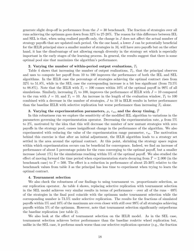
generate slight drop-off in performance from the J = 30 benchmark. The fraction of strategies over allruns achieving the optimum goes down from 32% to 27-28%. The reason for this difference between IELand SEL is that, when using realized payoffs only, the change in J does not affect the actual number ofstrategy payoffs that are updated each period. On the one hand, a lower J can be potentially beneficialfor the IELR principal since a smaller number of strategies inMt will have zero payoffs but on the otherhand, it has the disadvantage of not allowing enough diversity in the strategy set which is especiallyimportant in the early stages of the learning process. In general, the results suggest that there is someoptimal pool size that maximizes the algorithm’s performance.

2. Varying the number of within-period output evaluations, T1Table 4 shows that increasing the number of output realizations, T1, that the principal observes

and uses to compute her payoff from 10 to 100 improves the performance of both the IEL and SELalgorithms. In the IELR case the percentage of strategies achieving the optimal contract rises from32% to 51.8%, while in the SEL case the corresponding increase is a bit less significant (from 73.5%to 88.8%). Note that the IELR with T1 = 100 comes within 10% of the optimal payoff in 99% of allsimulations. Similarly, increasing T1 to 100, improves the performance of IELR with J = 10 comparedto the run with J = 10, and T1 = 10. An increase in the length of the evaluation window, T1 to 100combined with a decrease in the number of strategies, J to 10 in IELR results in better performancethan the baseline IELR with selective replication but worse performance than increasing T1 alone.

3. Varying the experimentation parameters, μ, rm, and the decay timing, TIn this robustness run we explore the sensitivity of the modified IEL algorithm to variations in the

parameters governing the experimentation operator. Decreasing the experimentation rate, μ from 5%to 2%, motivated by the idea that this will decrease the number of new mutant strategies with zeropayoffs in the strategy pool, causes insignificant change in the performance of the algorithm. We alsoexperimented with reducing the value of the experimentation range parameter, rm. The motivationbehind this exercise is that after an initial adjustment, the IELR algorithm leads to a strategy setsettled in the area around the optimal contract. At this point, shrinking the strategy space regionwithin which experimentation occurs can be beneficial for convergence. Indeed, we find an increase ofperformance of about 5 percentage points for the runs converging to the optimal payoff, but a smallerincrease (about 1%) for the simulations reaching within 5% of the optimal payoff. We also studied theeffect of moving forward the time period when experimentation starts decaying from T = 2, 000 (in thebenchmark case) to T = 500. The effect is a reduction in performance of about 25-30% relative to thebenchmark values from table 3 as the principal has less time to experiment when trying to learn theoptimal contract.

4. Tournament selectionWe also check the robustness of our findings to using tournament vs. proportionate selection, as

our replication operator. As table 4 shows, replacing selective replication with tournament selectionin the SEL model achieves very similar results in terms of performance — over all of the runs — 69%of the strategies in the final pool coincide with the optimum under tournament selection while thecorresponding number is 73.5% under selective replication. The results for the fractions of simulatedpayoffs within 5% and 10% of the maximum are even closer with still over 99% of all strategies achievingpayoffs within 5% of the optimum. However, note that tournament selection significantly outperformsthe baseline replication (see table 2).

We also look at the effect of tournament selection on the IELR model. As in the SEL case,tournament selection achieves better performance than the baseline roulette wheel replication but,unlike in the SEL case, it performs much worse than our selective replication operator (e.g., the fraction

18

of runs converging to the optimal contract falls from 32% to 2.6%). The reason for superior performanceof selective replication is that new mutants and unplayed strategies have zero payoffs. Such strategiesare replicated less frequently with selective replication than with tournament selection. This results inmore successful adaptation with selective replication.

5. The fitness weights, λWe also experimented with increasing the value of the parameter λ which governs the curvature in

the mapping between the average profits and the strategy fitness. The results from increasing λ from1 to 3 show a slight deterioration in performance (the average percentage over all runs of last periodstrategies coinciding with the optimum declines from 32% to 27%). Using the biased roulette wheelreplication from (9), a higher λ implies a higher probability of choosing a strategy with a high payoff.This may be beneficial later on when (or, if) we are close to the optimum but may lead to the strategiesin the pool being “stuck” far away from the optimum in the early stages of the learning process. Thecombination of these two effects accounts for the observed outcome30.

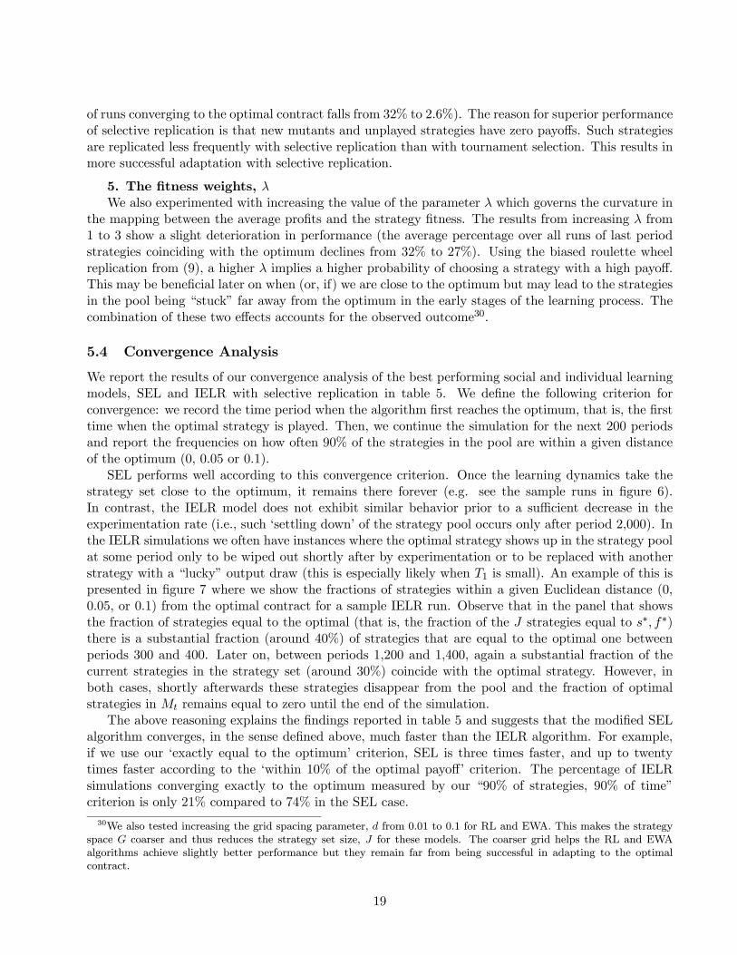
5.4 Convergence Analysis

We report the results of our convergence analysis of the best performing social and individual learningmodels, SEL and IELR with selective replication in table 5. We define the following criterion forconvergence: we record the time period when the algorithm first reaches the optimum, that is, the firsttime when the optimal strategy is played. Then, we continue the simulation for the next 200 periodsand report the frequencies on how often 90% of the strategies in the pool are within a given distanceof the optimum (0, 0.05 or 0.1).

SEL performs well according to this convergence criterion. Once the learning dynamics take thestrategy set close to the optimum, it remains there forever (e.g. see the sample runs in figure 6).In contrast, the IELR model does not exhibit similar behavior prior to a sufficient decrease in theexperimentation rate (i.e., such ‘settling down’ of the strategy pool occurs only after period 2,000). Inthe IELR simulations we often have instances where the optimal strategy shows up in the strategy poolat some period only to be wiped out shortly after by experimentation or to be replaced with anotherstrategy with a “lucky” output draw (this is especially likely when T1 is small). An example of this ispresented in figure 7 where we show the fractions of strategies within a given Euclidean distance (0,0.05, or 0.1) from the optimal contract for a sample IELR run. Observe that in the panel that showsthe fraction of strategies equal to the optimal (that is, the fraction of the J strategies equal to s∗, f∗)there is a substantial fraction (around 40%) of strategies that are equal to the optimal one betweenperiods 300 and 400. Later on, between periods 1,200 and 1,400, again a substantial fraction of thecurrent strategies in the strategy set (around 30%) coincide with the optimal strategy. However, inboth cases, shortly afterwards these strategies disappear from the pool and the fraction of optimalstrategies in Mt remains equal to zero until the end of the simulation.

The above reasoning explains the findings reported in table 5 and suggests that the modified SELalgorithm converges, in the sense defined above, much faster than the IELR algorithm. For example,if we use our ‘exactly equal to the optimum’ criterion, SEL is three times faster, and up to twentytimes faster according to the ‘within 10% of the optimal payoff’ criterion. The percentage of IELRsimulations converging exactly to the optimum measured by our “90% of strategies, 90% of time”criterion is only 21% compared to 74% in the SEL case.

30We also tested increasing the grid spacing parameter, d from 0.01 to 0.1 for RL and EWA. This makes the strategyspace G coarser and thus reduces the strategy set size, J for these models. The coarser grid helps the RL and EWAalgorithms achieve slightly better performance but they remain far from being successful in adapting to the optimalcontract.

19

We also analyze the IELR and SEL convergence rates as a function of the structural parametersγ and σ in the underlying economic model. This is shown in figure 8. The figure depicts the fraction(out of the 70 random seed runs for any fixed parameter pair) of non-convergent simulations (accordingto our criterion above) for the different values of the risk aversion parameter, γ and the variance ofoutput, σ that we use. Higher output variance, σ2 clearly hampers convergence. The intuition is thatfor a fixed number of output observations (T1) the principal has a harder time assigning a theoreticallycorrect payoff to a strategy that was played, and thus “lucky” sub-optimal strategies can outperformthe optimal one in case the latter obtains a bad sequence of output draws. The role of risk aversion,γ, on convergence is not so unambiguous but there is some evidence in the figures that higher riskaversion γ makes the convergence in payoffs relatively harder.

6 Discussion on Non-Convergence

In this section we discuss in more detail the reasons for the non-convergence of the individual evolution-ary learning algorithm in a large fraction of runs for both the benchmark and the modified algorithms.At first glance our finding that the standard IEL model with foregone payoffs virtually never convergesto the optimal strategy seems surprising as this algorithm has been previously shown to converge fastin numerous environments (e.g., Arifovic and Ledyard, 2004, 2007). In these environments, hypotheti-cal payoff evaluations are actually very helpful in achieving fast convergence. Foregone payoffs play auseful role in the algorithm’s ability to dismiss strategies that perform poorly. Foregone payoffs alsohelp in quickly evaluating strategies that are brought in via experimentation — only strategies that arepromising in terms of foregone payoffs are kept and replicated.

However, our principal-agent problem is different and, to some extent more complex than theenvironments in which IEL has been previously used. As we already pointed out, the main problemwith IEL’s adaptation comes from the sequential nature of our theoretical setting. According to thealgorithm, in order to evaluate a foregone payoff of a strategy that was not actually used, the principalassumes that the agent’s action would remain constant for any other strategy played. This is correct ina simultaneous-game (Nash) setting where each player is playing against a fixed strategy distribution.However, in our model — and in any similar principal-agent or sequential-play model for that matter —different principal’s strategies in fact result in different optimal actions by the agent. Under IEL, thewhole collection of strategies (actually played or hypothetical) is evaluated holding the agent’s actionconstant. Clearly, principals who use such learning algorithm and thus ignore the direct incentiveeffects of their actions would not be able to learn the optimal contract.

Even with the modifications of selective replication and realized payoffs evaluation we found thatthe IEL algorithm still experiences difficulties in learning the optimal contract in comparison to SEL.We discuss the possible reasons next. To begin with, remember that the randomly generated strategiesthat comprise the initial period strategy set are assigned zero payoffs31. In addition, any new strategygenerated during the simulation via experimentation is also assigned zero payoff. Strategies that violatethe participation constraint are also assigned zero payoffs. Those strategies that satisfy the participationconstraint can receive positive payoffs only once they have been played. However, strategies with zeropayoffs will always have a positive probability of being replicated, and unless they are replaced by astrategy with a positive payoff, they may remain idle in the principal’s strategy set for a long time.

Our direct visual observations of the learning process for many sample runs indicate that it takesa fairly long time for the IELR algorithm to eliminate most of the strategies that do not satisfy the

31The fact that the payoff is zero is not important per se. What is important is that all these strategies have the samepayoff.

20

participation constraint. When most of the strategies are on the “correct” side of the constraint,the algorithm displays improvement in performance in terms of strategy payoffs and closeness to theoptimal contract. This is displayed in figures 9 and 10 which illustrate and compare the evolutionof the strategy set, Mt, for the best performing individual and social learning models, namely SELwith selective replication (figure 9) and IELR with selective replication (figure 10). The figures plot,in strategy (s, f) space, the current strategies in the set (the circles) at various time periods and theparticipation constraint, for the same sample run. The diamond denotes the currently played strategyfor IELR, and the star denotes the optimal contract. We see that the better performance of the sociallearning model is due to the fact that it weeds out strategies that violate the participation constraintquite fast and then converges quickly and stays close to the optimum. In contrast, IELR exhibits‘cycles’, i.e., the strategies get close to the optimum but then the set spreads out again. It is only onceexperimentation decays sufficiently that IELR converges to the currently best strategy in Mt which,however, is not necessarily the optimal one.

The main problem with IELR and the reason for the behavior exhibited in figure 10 is that, even ifthe optimal strategy appears in the pool at some t, it can, at any later point in time, disappear from it.This decreases the probability that the algorithm converges to the optimal contract in any fixed numberof periods. To see this more clearly, suppose that the optimal strategy were present in the principal’sstrategy set at some period. One way through which it can be replaced by some different strategy isvia experimentation. A second possibility is for it to be replaced by some suboptimal strategy. Thelatter can happen in two ways: (1) because a suboptimal strategy was actually played and receivedhigher payoff than the optimal strategy that was never played (note this cannot happen in SEL as allstrategies inMt are played before updating); or (2) because a suboptimal strategy was “lucky” and gota series of favorable output draws which resulted in a payoff higher than the payoff that the optimalstrategy earned the last time it was played (this is less likely to happen in SEL where multiple copiesof the optimal strategy would be present in Mt). In both cases, if the number of other replicates ofthe optimal strategy in the collection is small or zero (much more likely for IELR than SEL), this canbe detrimental. The chance of bringing the optimal strategy back into the strategy pool, especiallytowards the end of a simulation run when we are either decreasing the radius of the experimentation,rm (or its rate, μ) is clearly diminishing to zero.

Similarly, given that under IELR not all strategies in the pool are evaluated each period (onlya single one is), previously ‘lucky’ strategies (those that have obtained high payoffs because of goodoutput draws) can persist in the pool while better strategies in terms of theoretically expected payoffscould be replaced. As the simulation is moving closer to the optimal contract in (s, f) space, because ofexperimentation, there might still be a number of points in the strategy pool outside of the participationconstraint, but close to the optimal and near-optimal strategies in the strategy space. This alsocontributes to IELR’s slow convergence or even the lack of convergence to the optimum.

The above discussion and evidence suggests that SEL focuses faster on a smaller number of strate-gies than the IELR. This point is further illustrated in figure 11 in which we report the frequencydistribution of all the strategies that were ‘active’ (played) during a given simulation. For each strat-egy in G we plot the number of times this strategy was ‘active’ divided by the total number of strategyevaluations that took place over the course of the simulation. Comparing the IELR vs. SEL panels,we see that the SEL simulation results in higher frequencies of fewer strategies that are concentratedaround the participation constraint and around the optimal strategy. At the same time, the IELR sim-ulation generates a much more spread-out distribution in which a larger number of dispersed strategiesincluding many on the ‘wrong’ side of the participation constraint were played.

Does the SEL algorithm perform better because N strategies (although not necessarily all different)

21

are evaluated per period while only a single strategy is evaluated in IELR each period? To put IELRon a more equal footing with SEL in terms of the total number of evaluated strategies, in figure 12 wecompare the make-up of the strategy sets at time periods for which the number of strategy evaluations inIELR roughly equals that in SEL32. More specifically, we run IELR for 30 (=N) times as many periodsas SEL (15,000 vs. 500) — for example, the top row of panels on figure 12 compares the strategy pool att = 200 for SEL with t = 6, 000 for IELR. Clearly, even with the same number of evaluations, the IELRstrategy set remains much more dispersed. Looking at the fraction of converging strategy under IELRover time, we see that after some initial progress, these fractions stabilize around 0.1 for strategiesequal to the optimum and around 0.25 for strategies within 0.05 away from the optimum and stay atthese levels until the end of a simulation.

These results reveal that, since SEL is different from simply ‘repeating’ IELR N times or alter-natively, an N -player version of IELR, the under-performance of individual learning in our setting isnot simply due to the number of strategy evaluations that are performed. What causes the differencein performance then? Remember, IELR updates (via replication and experimentation) each time astrategy is played, while SEL updates once all N strategies in Mt are played. Thus SEL uses moreinformation to update the strategy set and experimentation occurs less often. In IELR, as shown above,zero-payoff strategies stay in the pool for a relatively long periods of time as they are unlikely to beselected to play because of their low fitness. of their low fitnnesses they are unlikely to get played. Incontrast, in SEL such strategies are played with certainty and weeded out quickly. One way to makeIELR perform like SEL would be to ‘force’ the principal to postpone replication and experimentationand instead play all her J (=N) current strategies before updating. However, there is no reason forthis to be optimal in general. Moreover, this major difference in SEL vs. IELR is not just a modelingassumption. Instead it is inherent to what these learning algorithms stand for — in SEL one, andeveryone, learns from one’s own and other people’s experiences while in IELR one learns from one’sown experience only. The physical time to updating is the same (every time period), however in IELRone (being alone) is able to play just a single strategy at a time, while in SEL N strategies are played.

7 Conclusions

We introduce learning in a principal-agent model and examine whether and what type of learning pro-cesses converge to the theoretically optimal agency contract. Solving for the optimal contract in suchmodels is often computationally difficult and may require a fair amount of knowledge about the envi-ronment by the principal. The learning models that we analyze are social evolutionary learning (SEL)and three different models of individual learning: reinforcement learning (RL), experience weightedattraction learning (EWA), and individual evolutionary learning (IEL). In addition, we introduce andevaluate a modified version of IEL that we call individual evolutionary learning with realized payoffs(IELR).

Our results show that learning in the principal-agent environment is very difficult. This is due tothree main reasons: (1) the stochastic environment, (2) the discontinuity in payoffs in a neighborhoodof the optimal contract due to the participation constraint and (3) incorrect evaluation of foregonepayoffs in the sequential game principal-agent setting. The first two factors apply to all the learningalgorithms that we study, while the third one is the main reason for the failure of the EWA andIEL models in our setting. In terms of the performance, we show that SEL (especially with selectivereplication) is the most successful in achieving convergence to the optimal contract. In contrast, the

32In fact, since the strategy pool under SEL typically contains several replicates of the same strategy, this exercise givesan advantage to IELR in terms of total number of strategy evaluations.

22

canonical versions of the individual learning algorithms (IEL, RL and EWA) fail to converge.To overcome the difficulties with convergence to the optimal contract for the individual learning

algorithm and remedy the problem of incorrect evaluation of foregone payoffs, we modified the IELalgorithm so that only the payoffs of strategies that are actually tried out are updated. This updatingrule is similar to that used in RL. However, we keep all other essential elements of the IEL updating,namely its replication and experimentation operators that enable IEL to handle environments withlarge strategy space much better than RL. The resulting hybrid algorithm (which we call IEL withrealized payoffs, IELR) is much more successful than all other individual learning models we studied.The implementation of selective replication improves its performance further. Nevertheless, our mainconclusion, based on numerous robustness checks and parametrizations, is that, in both the canonicalalgorithms and their modified versions, principals who are learning from each other can achieve muchbetter results than principals who only learn on their own. Our results thus echo the famous quotefrom Marshall’s (1920) Principles of Economics: “If one man starts new idea, it is taken up by othersand combined with suggestions of their own; and thus becomes the source of new ideas”.

More generally, our findings suggest that the relatively simple learning rules we evaluate in this pa-per, despite having proved successful in many normal form game settings (largely based on Nash play)or various macroeconomic settings, may not be well-suited for the sequential strategic problems of struc-turing incentives that arise in the principal-agent models. Our results suggest that these environmentsmight require much more sophisticated principals in terms of the knowledge about the environmentthey operate in, for example, about the nature of the participation and incentive constraints, the natureof the stochastic process that the technology is subject to and degree to which agents’ are risk averse.Correct implementation of this knowledge would also require greater computational ability than whatour boundedly rational agents are endowed with.33

We chose a one-sided learning framework for its tractability and to isolate better the relativeperformance of the various learning algorithms. Naturally, ours is thus a partial characterization of thereal-world principal-agent environments where both sides can continuously and simultaneously learnfrom each other. While this remains outside the scope of this paper, we conjecture that allowing fordouble-sided learning in our setting is likely to make the performance of the algorithms worse. Indeed,due to the one-shot structure of our principal-agent game with the agent playing last, there is nostrategic advantage to the agent of being fully rational — she cannot ‘manipulate’ to her benefit theprincipal’s choice of (s, f) and make the principal deviate from the optimal contract. Thus, modelingthe agent as fully rational does not make learning harder for the principal. On the contrary, if theagents were also boundedly rational and learning about how much effort to supply, then for example,choosing an incorrect level of effort may lead the principal to pick ‘wrong’ contracts which is likely toslow the learning process for both parties. Finally, making the agents learn about their optimal effort, zwould not make the problem of incorrect evaluation of hypothetical payoffs disappear. Remember, thenature of that problem lies in the principal’s taking the agent’s reaction to any other contract offeredas fixed. We know that a fully rational agent varies his effort one-to-one with the share s and there isno reason that a learning agent would not vary his effort with different offered contracts as well. Aslong as the latter is the case, EWA or IEL would fail also with two-sided learning.

How could we test our results empirically? As a first step, we plan to use experiments withhuman subjects. We are developing an experimental design for two types of environments. In thefirst environment, subjects (who play the role of the principals in the model) will learn from theirown experience only. In the second environment, subjects will be given a chance to interact with other

33Designing a learning model with just the ‘right’ amount of sophistication necessary for successful adaptation in suchsettings is on our future research agenda.

23

subjects and exchange ideas of what the best strategies are. Given sufficient experimental or other data,we can formally test and distinguish statistically between the social and individual learning models34.IEL agents learn from their own experience and therefore only the time they have spent on the task(plus maybe an idiosyncratic shock or fixed effect) should affect how well they perform. In contrast,SEL agents learn from others, in addition to what they can achieve on their own. Thus how manyother agents one is in contact with (e.g. data on social networks, friends, neighbors, etc.) should affecttheir performance, in addition to their own experience. That is, both the strength of the relationshipsan agent has with others and their number should influence her outcome under SEL but not underIEL.

In future work we plan to apply the basic framework and methodology laid down here to otherprincipal-agent settings. We have already studied an application to an adverse selection environment(Arifovic and Karaivanov, 2009) and intend to develop an application to a dynamic models of asym-metric information (e.g. as in the optimal taxation or optimal insurance literatures).

References

[1] Arifovic, J. (1994), “Genetic Algorithm and the Cobweb Model”, Journal of Economic Dynamicsand Control, 18, pp. 3-28.

[2] Arifovic, J. (1996), “The Behavior of the Exchange Rate in the Genetic Algorithm and Experi-mental Economies ”, Journal of Political Economy, 104, 510-541.

[3] Arifovic, J. (2000), “Evolutionary Algorithms in Macroeconomic Modeling: A Survey ”, Macroe-conomic Dynamics 4, pp. 373-414.

[4] Arifovic, J. and A. Karaivanov (2009), “Social Learning in a Model of Adverse Selection”, forth-coming in D. West, G. Dow, and A. Eckert (eds.), Essays in Honour of B. Curtis Eaton, Universityof Toronto Press

[5] Arifovic, J. and J. Ledyard (2004), “Scaling Up Learning Models in Public Good Games, Journalof Public Economic Theory 6, pp. 205-38.

[6] Arifovic, J. and J. Ledyard (2007) “Call Market Book Information and Efficiency ”, Journal ofEconomic Dynamics and Control, 31, pp. 1971-2000.

[7] Arifovic J. and M. Maschek (2006) “Revisiting Individual Evolutionary Learning in the CobwebModel. An Illustration of the Virtual Spite-Effect”, Computational Economics, 28, pp. 333-354.

[8] Arrow, K. (1962) “The Economic Implications of Learning by Doing ”, Review of Economic Stud-ies, 29, pp. 155-73.

[9] Arrow, K. (1985), “Informational Structure of the Firm”, American Economic Review, 75(2), pp.303-07.

[10] Bolton, P. and M. Dewatripont (2005), Contract Theory, The MIT Press, Cambridge, MA.

[11] Boyd, J. and R. Bresser (2004), “Momentum, Imitation, and Learning: Evidence from and Effectson the U.S. Retail Industry”, working paper, Free University Berlin.

34For example, we can use the maximum likelihood based model comparison approach of Karaivanov and Townsend(2009).

24

[12] Camerer, C. (2003), Behavioral Game Theory: Experiments in Strategic Interaction, PrincetonUniversity Press, Princeton, NJ.

[13] Camerer, C. and T. Ho (1999), “Experience Weighted Attraction Learning in Normal FormGames”, Econometrica 67, pp. 167-88.

[14] Caves, R., Crookell, H., and Killing, J. (1983), “The Imperfect Market for Technology Licenses”,Oxford Bulletin of Economics and Statistics, 45, pp. 249-67.

[15] Chao, K. (1983), “Tenure Systems in Traditional China”, Economic Development and CulturalChange 31, pp. 295-314.

[16] Conley, T. and C. Udry (2005), “Learning About a New Technology: Pineapple in Ghana”, workingpaper, University of Chicago.

[17] Cunningham, R. (2004), “Investment, Private Information, and Social Learning: A Case Study ofthe Semiconductor Industry”, Bank of Canada Working Paper #2004-32.

[18] Dawid, H. (1999), Adaptive Learning by Genetic Algorithms: Analytical Results and Applicationsto Economic Models, 2nd revised and extended edition, Springer, Berlin.

[19] Dutta, S. and X. Zhang (2002), “Revenue Recognition in a Multiperiod Agency Setting”, Journalof Accounting Research 40, pp. 67-83.

[20] Erev, I. and Haruvy, E. (2008), “Learning and the Economics of Small Decisions ”, Handbook ofExperimental Economics, vol. 2, J. Kagel and A. Roth (eds.), forthcoming.

[21] Erev, I. and A. Roth (1998), “Predicting How People Play Games: Reinforcement Learning inExperimental Games with Unique, Mixed Strategy Equilibria ”, American Economic Review 88,pp. 848-81.

[22] Foster, A. and M. Rosenzweig (1996), ”Learning by Doing and Learning from Others: HumanCapital and Technical Change in Agriculture”, American Economic Review 103(6), pp. 1176-1209.

[23] Fudenberg, D. and D. Levine (1998) “The Theory of Learning in Games”, in Series on EconomicLearning and Social Evolution, vol. 2, MIT Press, Cambridge, MA.

[24] Hart, O. and B. Holmstrom (1987), “The Theory of Contracts” in T. Bewley (ed.), Advances inEconomic Theory, Cambridge University Press.

[25] Holmstrom, B. (1979), “Moral Hazard and Observability”, Bell Journal of Economics, 10(1), pp.74-91.

[26] Holmstrom, B. and P. Milgrom (1987), “Aggregation and Linearity in the Provision of Intertem-poral Incentives”, Econometrica 55, pp. 303-28.

[27] Holmstrom, B. and P. Milgrom (1991), “Multitask Principal-Agent Analyses: Incentive Contracts,Asset Ownership, and Job Design”, Journal of Law, Economics and Organisation, 7, pp. 24-52.

[28] Hommes, C. and T. Lux (2008), “Individual Learning, Heterogeneity and Aggregate Behavior inCobweb Experiments ”, manuscript.

25

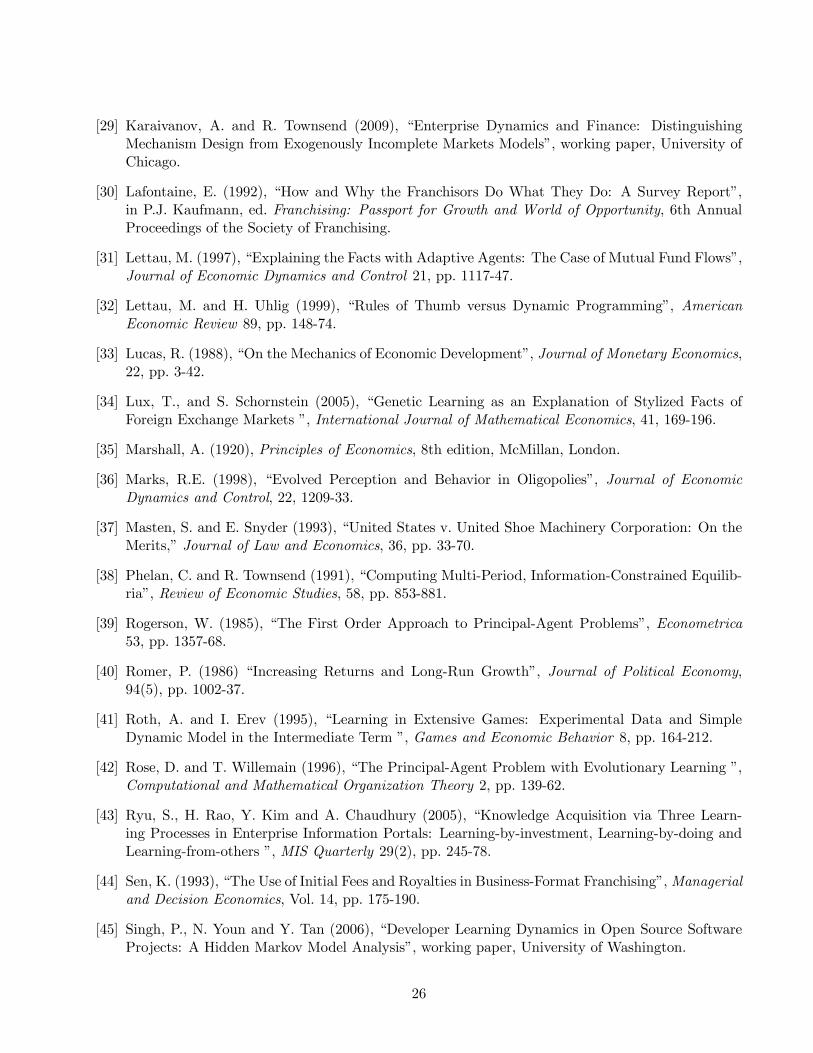
[29] Karaivanov, A. and R. Townsend (2009), “Enterprise Dynamics and Finance: DistinguishingMechanism Design from Exogenously Incomplete Markets Models”, working paper, University ofChicago.

[30] Lafontaine, E. (1992), “How and Why the Franchisors Do What They Do: A Survey Report”,in P.J. Kaufmann, ed. Franchising: Passport for Growth and World of Opportunity, 6th AnnualProceedings of the Society of Franchising.

[31] Lettau, M. (1997), “Explaining the Facts with Adaptive Agents: The Case of Mutual Fund Flows”,Journal of Economic Dynamics and Control 21, pp. 1117-47.

[32] Lettau, M. and H. Uhlig (1999), “Rules of Thumb versus Dynamic Programming”, AmericanEconomic Review 89, pp. 148-74.

[33] Lucas, R. (1988), “On the Mechanics of Economic Development”, Journal of Monetary Economics,22, pp. 3-42.

[34] Lux, T., and S. Schornstein (2005), “Genetic Learning as an Explanation of Stylized Facts ofForeign Exchange Markets ”, International Journal of Mathematical Economics, 41, 169-196.

[35] Marshall, A. (1920), Principles of Economics, 8th edition, McMillan, London.

[36] Marks, R.E. (1998), “Evolved Perception and Behavior in Oligopolies”, Journal of EconomicDynamics and Control, 22, 1209-33.

[37] Masten, S. and E. Snyder (1993), “United States v. United Shoe Machinery Corporation: On theMerits,” Journal of Law and Economics, 36, pp. 33-70.

[38] Phelan, C. and R. Townsend (1991), “Computing Multi-Period, Information-Constrained Equilib-ria”, Review of Economic Studies, 58, pp. 853-881.

[39] Rogerson, W. (1985), “The First Order Approach to Principal-Agent Problems”, Econometrica53, pp. 1357-68.

[40] Romer, P. (1986) “Increasing Returns and Long-Run Growth”, Journal of Political Economy,94(5), pp. 1002-37.

[41] Roth, A. and I. Erev (1995), “Learning in Extensive Games: Experimental Data and SimpleDynamic Model in the Intermediate Term ”, Games and Economic Behavior 8, pp. 164-212.

[42] Rose, D. and T. Willemain (1996), “The Principal-Agent Problem with Evolutionary Learning ”,Computational and Mathematical Organization Theory 2, pp. 139-62.

[43] Ryu, S., H. Rao, Y. Kim and A. Chaudhury (2005), “Knowledge Acquisition via Three Learn-ing Processes in Enterprise Information Portals: Learning-by-investment, Learning-by-doing andLearning-from-others ”, MIS Quarterly 29(2), pp. 245-78.

[44] Sen, K. (1993), “The Use of Initial Fees and Royalties in Business-Format Franchising”,Managerialand Decision Economics, Vol. 14, pp. 175-190.

[45] Singh, P., N. Youn and Y. Tan (2006), “Developer Learning Dynamics in Open Source SoftwareProjects: A Hidden Markov Model Analysis”, working paper, University of Washington.

26

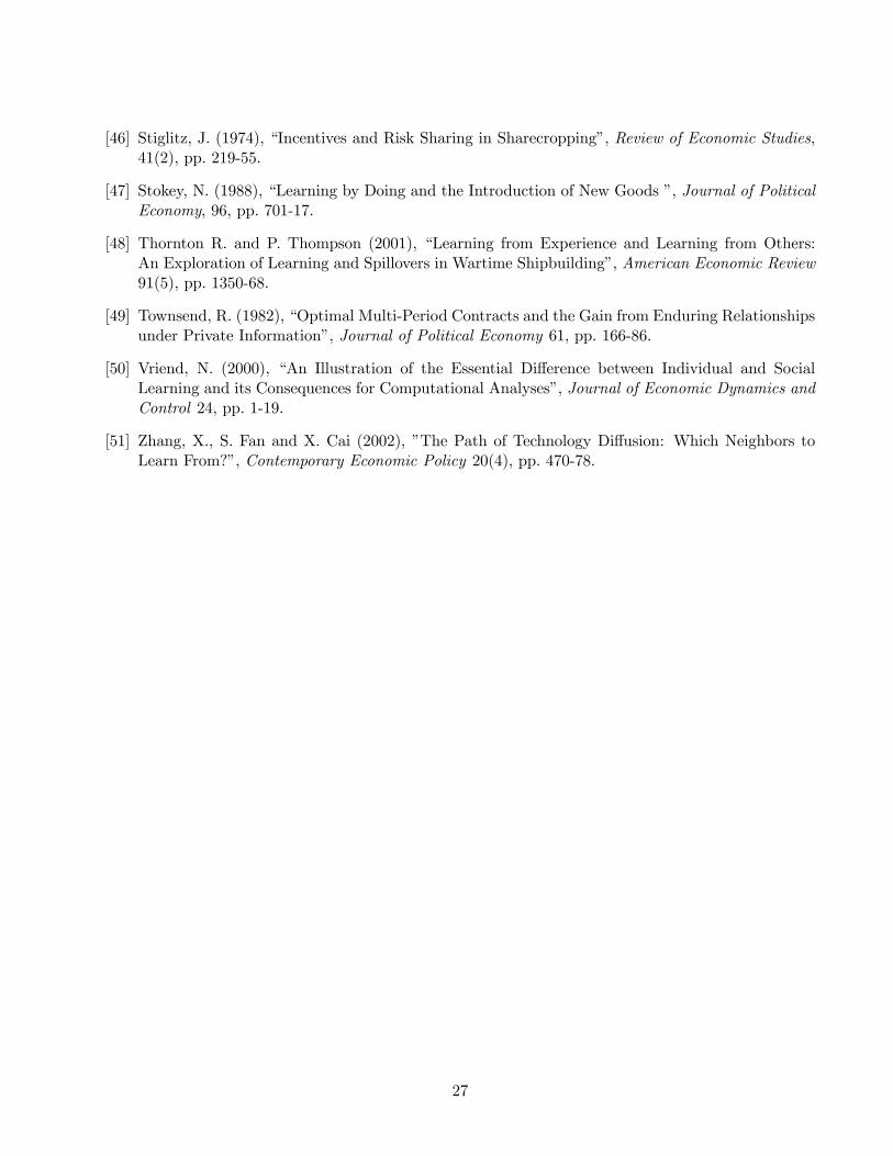
[46] Stiglitz, J. (1974), “Incentives and Risk Sharing in Sharecropping”, Review of Economic Studies,41(2), pp. 219-55.

[47] Stokey, N. (1988), “Learning by Doing and the Introduction of New Goods ”, Journal of PoliticalEconomy, 96, pp. 701-17.

[48] Thornton R. and P. Thompson (2001), “Learning from Experience and Learning from Others:An Exploration of Learning and Spillovers in Wartime Shipbuilding”, American Economic Review91(5), pp. 1350-68.

[49] Townsend, R. (1982), “Optimal Multi-Period Contracts and the Gain from Enduring Relationshipsunder Private Information”, Journal of Political Economy 61, pp. 166-86.

[50] Vriend, N. (2000), “An Illustration of the Essential Difference between Individual and SocialLearning and its Consequences for Computational Analyses”, Journal of Economic Dynamics andControl 24, pp. 1-19.

[51] Zhang, X., S. Fan and X. Cai (2002), ”The Path of Technology Diffusion: Which Neighbors toLearn From?”, Contemporary Economic Policy 20(4), pp. 470-78.

27

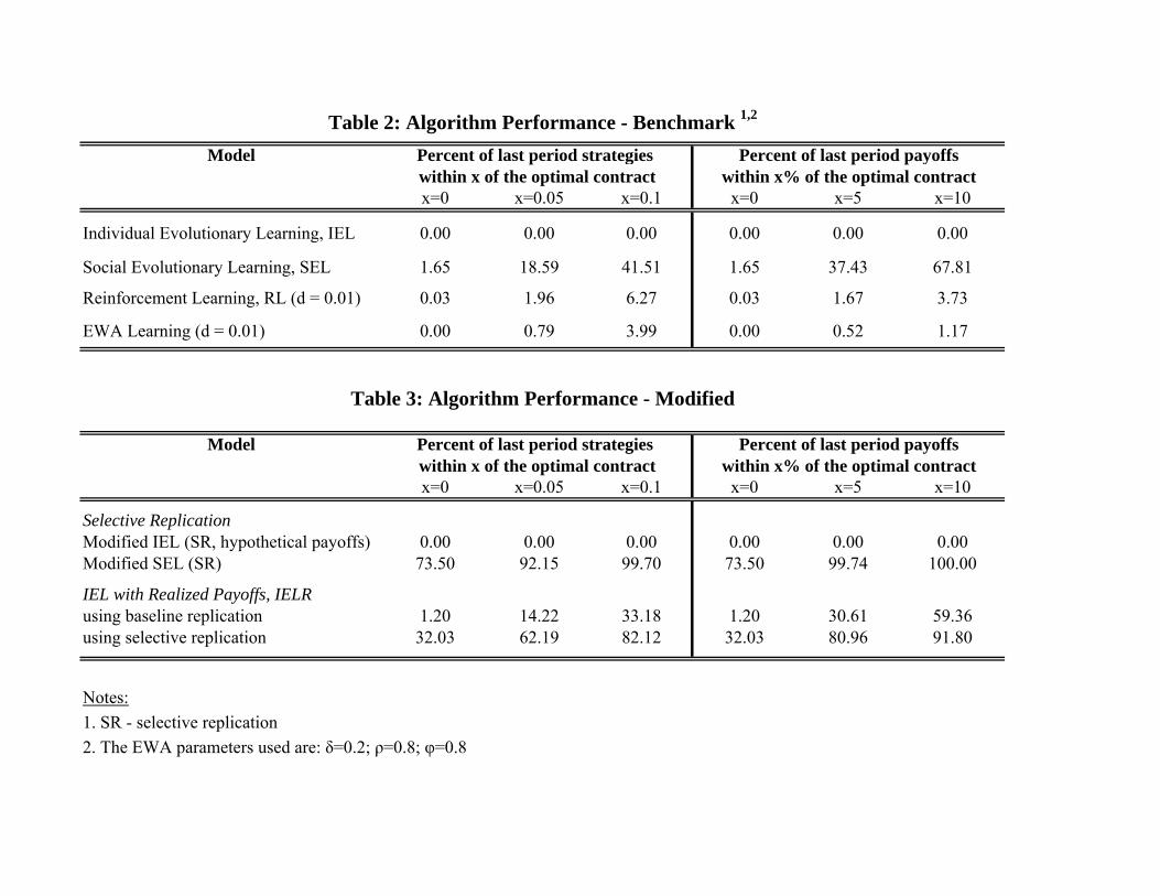
Model

x=0 x=0.05 x=0.1 x=0 x=5 x=10

Individual Evolutionary Learning, IEL 0.00 0.00 0.00 0.00 0.00 0.00

Social Evolutionary Learning, SEL 1.65 18.59 41.51 1.65 37.43 67.81

Reinforcement Learning, RL (d = 0.01) 0.03 1.96 6.27 0.03 1.67 3.73

EWA Learning (d = 0.01) 0.00 0.79 3.99 0.00 0.52 1.17

Model

x=0 x=0.05 x=0.1 x=0 x=5 x=10

Selective ReplicationModified IEL (SR, hypothetical payoffs) 0.00 0.00 0.00 0.00 0.00 0.00Modified SEL (SR) 73.50 92.15 99.70 73.50 99.74 100.00

IEL with Realized Payoffs, IELRusing baseline replication 1.20 14.22 33.18 1.20 30.61 59.36using selective replication 32.03 62.19 82.12 32.03 80.96 91.80

Notes:1. SR - selective replication2. The EWA parameters used are: δ=0.2; ρ=0.8; φ=0.8

Percent of last period strategies Percent of last period payoffs

Table 2: Algorithm Performance - Benchmark 1,2

within x of the optimal contract within x% of the optimal contract

Table 3: Algorithm Performance - Modified

Percent of last period strategies Percent of last period payoffswithin x of the optimal contract within x% of the optimal contract

Model

x=0 x=0.05 x=0.1 x=0 x=5 x=10

Individual (SR, N=100) 27.66 57.84 78.40 27.66 74.94 84.80Individual (SR, N=10) 26.88 56.97 78.69 26.88 77.63 89.06Individual (SR, T1=100) 51.77 78.72 94.95 51.77 94.91 98.97Individual (SR, N=10, T1=100) 42.22 71.77 91.44 42.22 92.48 98.34Individual (SR, experimentation rate=0.02) 32.61 63.14 83.94 32.61 82.56 92.44Individual (SR, perturbation radius decay) 37.26 67.28 88.18 37.26 85.17 94.50Individual (SR, early experimentation decay) 18.94 44.93 67.54 18.94 77.99 90.95Individual (tournament selection) 2.59 13.03 26.52 2.59 41.76 62.07Individual (SR, λ=3) 27.09 59.96 81.48 27.09 78.92 88.97

Social (SR, N=100) 89.70 98.94 100.00 89.70 100.00 100.00Social (SR, T1=100) 88.75 98.71 100.00 88.75 100.00 100.00Social (SR, early experimentation decay) 48.57 64.04 84.60 48.57 97.54 99.77Social (tournament selection) 68.90 90.12 99.13 68.90 99.25 99.99

Notes:1. SR - selective replication2. All individual runs use realized payoffs only (IELR)

Percent of last period strategies Percent of last period payoffs

Table 4: Algorithm Performance - Robustness Checks 1,2

within x of the optimal contract within x% of the optimal contract

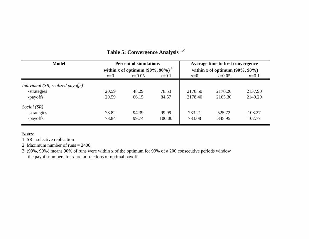
Model

x=0 x=0.05 x=0.1 x=0 x=0.05 x=0.1

Individual (SR, realized payoffs) -strategies 20.59 48.29 78.53 2178.50 2170.20 2137.90 -payoffs 20.59 66.15 84.57 2178.40 2165.30 2149.20

Social (SR) -strategies 73.82 94.39 99.99 733.21 525.72 108.27 -payoffs 73.84 99.74 100.00 733.08 345.95 102.77

Notes:1. SR - selective replication2. Maximum number of runs = 24003. (90%, 90%) means 90% of runs were within x of the optimum for 90% of a 200 consecutive periods window the payoff numbers for x are in fractions of optimal payoff

Percent of simulations Average time to first convergence

Table 5: Convergence Analysis 1,2

within x of optimum (90%, 90%) 3 within x of optimum (90%, 90%)

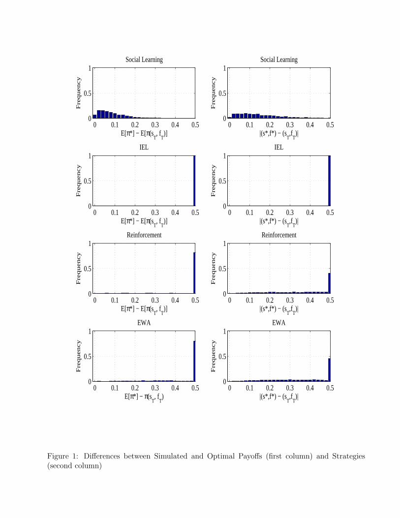
0 0.1 0.2 0.3 0.4 0.50

0.5

1Social Learning

E[π*] − E[π(sT, f

T)]

Fre

qu

en

cy

0 0.1 0.2 0.3 0.4 0.50

0.5

1Social Learning

|(s*,f*) − (sT,f

T)|

Fre

qu

en

cy

0 0.1 0.2 0.3 0.4 0.50

0.5

1IEL

E[π*] − E[π(sT, f

T)]

Fre

qu

en

cy

0 0.1 0.2 0.3 0.4 0.50

0.5

1IEL

|(s*,f*) − (sT,f

T)|

Fre

qu

en

cy

0 0.1 0.2 0.3 0.4 0.50

0.5

1Reinforcement

E[π*] − E[π(sT, f

T)]

Fre

qu

en

cy

0 0.1 0.2 0.3 0.4 0.50

0.5

1Reinforcement

|(s*,f*) − (sT,f

T)|

Fre

qu

en

cy

0 0.1 0.2 0.3 0.4 0.50

0.5

1EWA

E[π*] − π(sT, f

T)

Fre

qu

en

cy

0 0.1 0.2 0.3 0.4 0.50

0.5

1EWA

|(s*,f*) − (sT,f

T)|

Fre

qu

en

cy

Figure 1: Differences between Simulated and Optimal Payoffs (first column) and Strategies(second column)

29

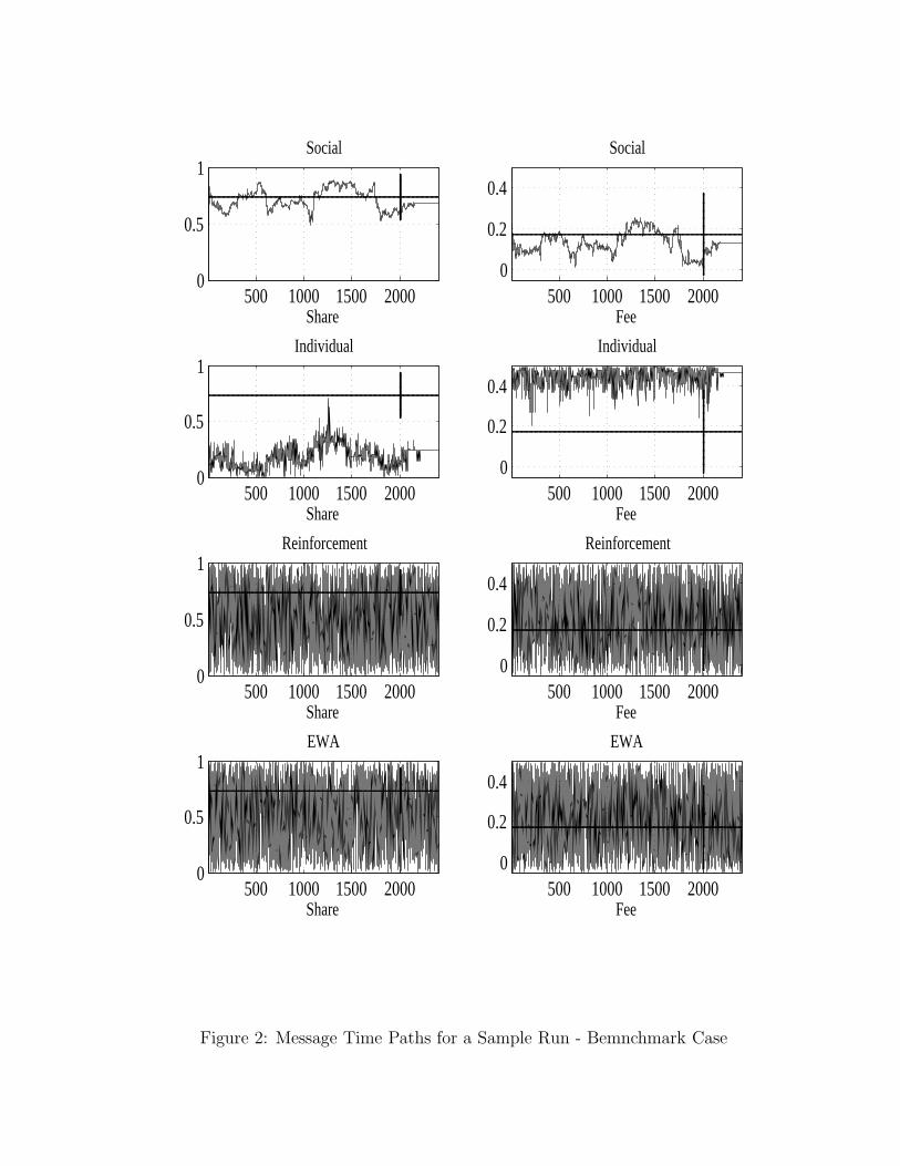
500 1000 1500 20000

0.5

1

Share

Social

500 1000 1500 20000

0.2

0.4

Fee

Social

500 1000 1500 20000

0.5

1

Share

Individual

500 1000 1500 20000

0.2

0.4

Fee

Individual

500 1000 1500 20000

0.5

1

Share

Reinforcement

500 1000 1500 20000

0.2

0.4

Fee

Reinforcement

500 1000 1500 20000

0.5

1

Share

EWA

500 1000 1500 20000

0.2

0.4

Fee

EWA

Figure 2: Message Time Paths for a Sample Run - Bemnchmark Case

30

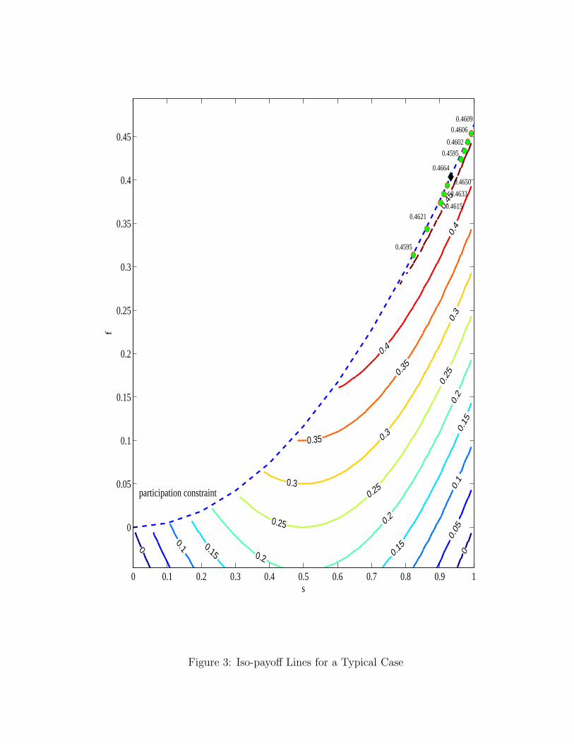
0

0

0.05

0.1

0.1

0.15 0.15

0.15

0.2

0.2

0.2

0.25

0.25

0.25

0.3

0.3

0.3

0.35

0.35

0.4

0.4

0.45

f

s

participation constraint

0 0.1 0.2 0.3 0.4 0.5 0.6 0.7 0.8 0.9 1

0

0.05

0.1

0.15

0.2

0.25

0.3

0.35

0.4

0.45

0.4664

0.4633

0.4595

0.4621

0.4650

0.4606

0.4595

0.4609

0.4615

0.4602

Figure 3: Iso-payoff Lines for a Typical Case

31

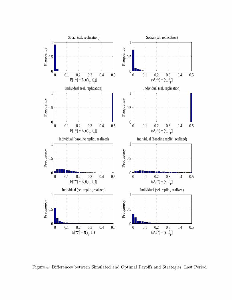
0 0.1 0.2 0.3 0.4 0.50

0.5

1Social (sel. replication)

E[π*] − E[π(sT, f

T)]

Fre

qu

en

cy

0 0.1 0.2 0.3 0.4 0.50

0.5

1Social (sel. replication)

|(s*,f*) − (sT,f

T)|

Fre

qu

en

cy

0 0.1 0.2 0.3 0.4 0.50

0.5

1Individual (sel. replication)

E[π*] − E[π(sT, f

T)]

Fre

qu

en

cy

0 0.1 0.2 0.3 0.4 0.50

0.5

1Individual (sel. replication)

|(s*,f*) − (sT,f

T)|

Fre

qu

en

cy

0 0.1 0.2 0.3 0.4 0.50

0.5

1Individual (baseline replic., realized)

E[π*] − E[π(sT, f

T)]

Fre

qu

en

cy

0 0.1 0.2 0.3 0.4 0.50

0.5

1Individual (baseline replic., realized)

|(s*,f*) − (sT,f

T)|

Fre

qu

en

cy

0 0.1 0.2 0.3 0.4 0.50

0.5

1Individual (sel. replic., realized)

E[π*] − π(sT, f

T)

Fre

qu

en

cy

0 0.1 0.2 0.3 0.4 0.50

0.5

1Individual (sel. replic., realized)

|(s*,f*) − (sT,f

T)|

Fre

qu

en

cy

Figure 4: Differences between Simulated and Optimal Payoffs and Strategies, Last Period

32

500 1000 1500 20000

0.5

1Social (sel. replication)

|(s*,r*) − (s,f)| <= x500 1000 1500 2000

0

0.5

1Social (sel. replication)

|E[π*] − E[π(s,f)]| <= x%

500 1000 1500 20000

0.5

1Individual (sel. replication)

|(s*,f*) − (s,f)| <= x500 1000 1500 2000

0

0.5

1Individual (sel. replication)

|E[π*] − E[π(s,f)]| <= x%

500 1000 1500 20000

0.5

1Individual (baseline replic., realized)

|(s*,f*) − (s,f)| <= x500 1000 1500 2000

0

0.5

1Individual (baseline replic., realized)

|E[π*] − E[π(s,f)]| <= x%

500 1000 1500 20000

0.5

1Individual (sel. replic., realized)

|(s*,f*) − (s,f)| <= x500 1000 1500 2000

0

0.5

1Individual (sel. replic., realized)

|E[π*] − E[π(s,f)]| <= x%

x=0x=0.05

x=0x=5

Figure 5: Time Paths of the Fraction of Simulated Strategies/Payoffs Equal to the Optimum(solid Line) and 5% of the Optimum (dotted Line)

33

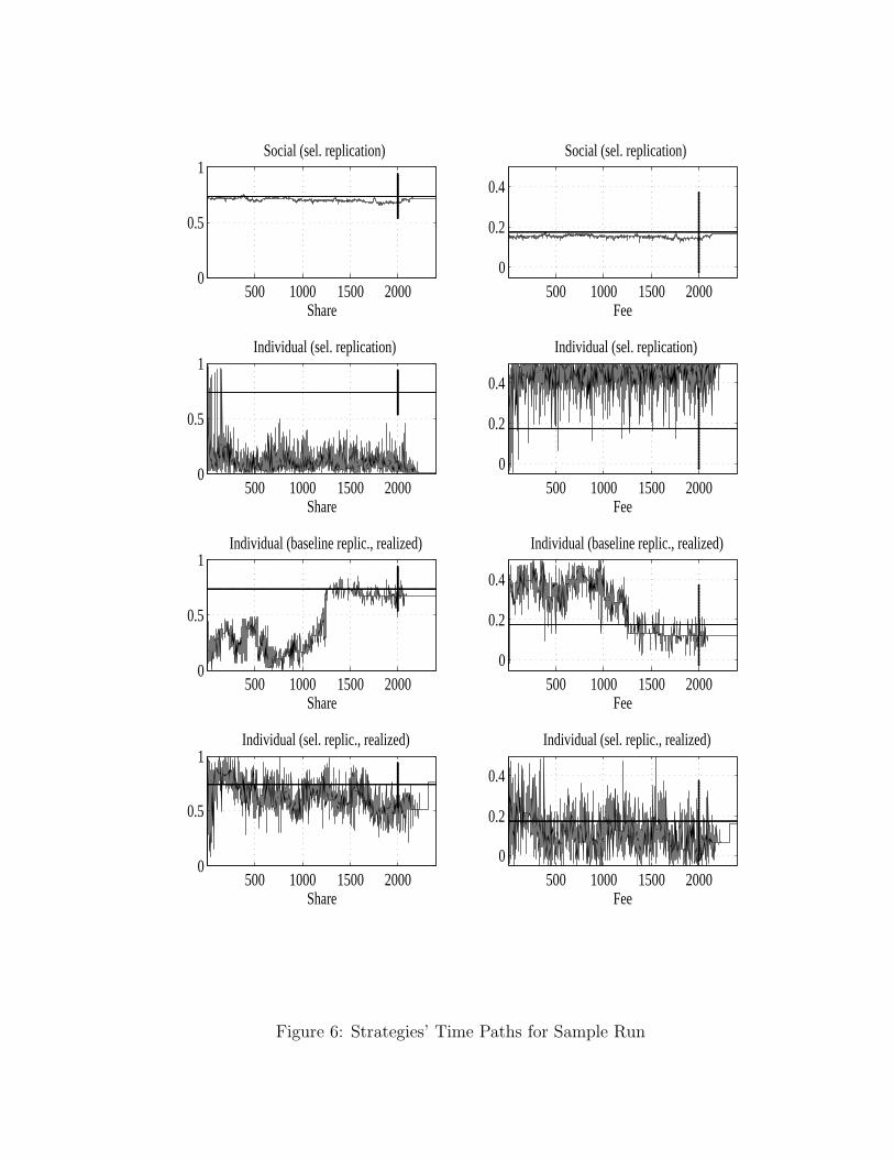
500 1000 1500 20000

0.5

1

Share

Social (sel. replication)

500 1000 1500 20000

0.2

0.4

Fee

Social (sel. replication)

500 1000 1500 20000

0.5

1

Share

Individual (sel. replication)

500 1000 1500 20000

0.2

0.4

Fee

Individual (sel. replication)

500 1000 1500 20000

0.5

1

Share

Individual (baseline replic., realized)

500 1000 1500 20000

0.2

0.4

Fee

Individual (baseline replic., realized)

500 1000 1500 20000

0.5

1

Share

Individual (sel. replic., realized)

500 1000 1500 20000

0.2

0.4

Fee

Individual (sel. replic., realized)

Figure 6: Strategies’ Time Paths for Sample Run

34

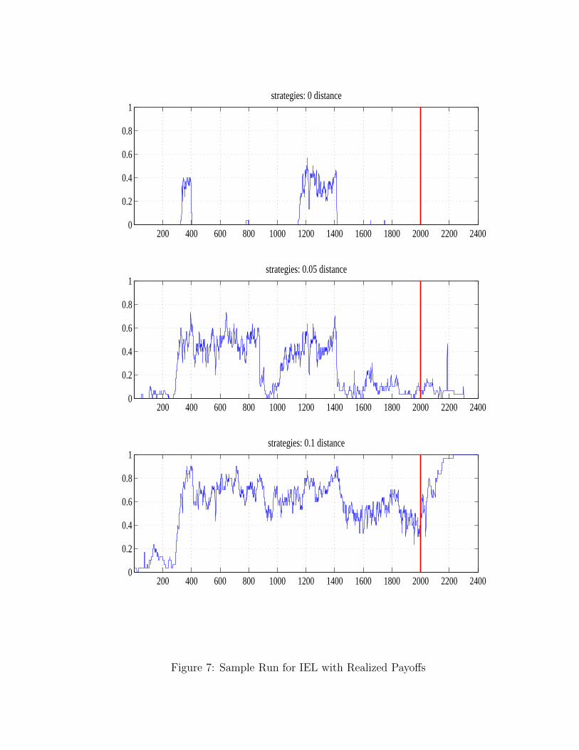
200 400 600 800 1000 1200 1400 1600 1800 2000 2200 24000

0.2

0.4

0.6

0.8

1strategies: 0 distance

200 400 600 800 1000 1200 1400 1600 1800 2000 2200 24000

0.2

0.4

0.6

0.8

1 strategies: 0.05 distance

200 400 600 800 1000 1200 1400 1600 1800 2000 2200 24000

0.2

0.4

0.6

0.8

1 strategies: 0.1 distance

Figure 7: Sample Run for IEL with Realized Payoffs

35

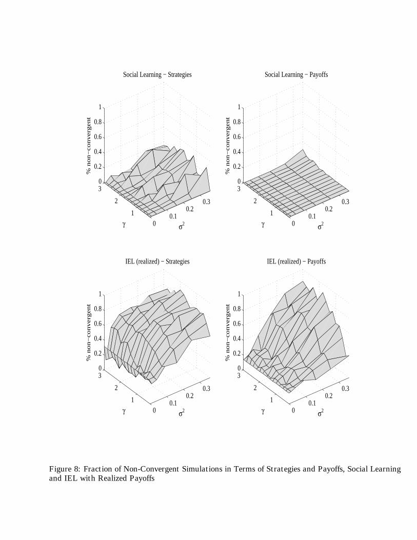
00.1

0.20.3

1

2

30

0.2

0.4

0.6

0.8

1

σ2

Social Learning − Strategies

γ

% n

on

−co

nv

erg

ent

00.1

0.20.3

1

2

30

0.2

0.4

0.6

0.8

1

σ2

Social Learning − Payoffs

γ%

no

n−

con

ver

gen

t

00.1

0.20.3

1

2

30

0.2

0.4

0.6

0.8

1

σ2

IEL (realized) − Strategies

γ

% n

on

−co

nv

erg

ent

00.1

0.20.3

1

2

30

0.2

0.4

0.6

0.8

1

σ2

IEL (realized) − Payoffs

γ

% n

on

−co

nv

erg

ent

Figure 8: Fraction of Non-Convergent Simulations in Terms of Strategies and Payoffs, Social Learningand IEL with Realized Payoffs

0 0.5 1

0

0.1

0.2

0.3

0.4

0.5Period = 1

s

f

0 0.5 1

0

0.1

0.2

0.3

0.4

0.5Period = 3

sf

0 0.5 1

0

0.1

0.2

0.3

0.4

0.5Period = 5

s

f

0 0.5 1

0

0.1

0.2

0.3

0.4

0.5Period = 100

s

f

0 0.5 1

0

0.1

0.2

0.3

0.4

0.5Period = 1000

s

f

0 0.5 1

0

0.1

0.2

0.3

0.4

0.5Period = 1500

s

f

0 0.5 1

0

0.1

0.2

0.3

0.4

0.5Period = 2000

s

f

0 0.5 1

0

0.1

0.2

0.3

0.4

0.5Period = 2100

s

f

0 0.5 1

0

0.1

0.2

0.3

0.4

0.5Period = 2400

s

f

Figure 9: Evolution of a Typical Run - Social Learning

37

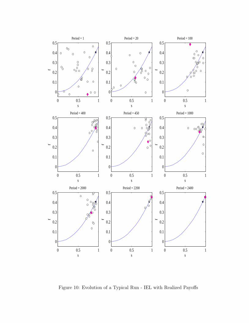
0 0.5 1

0

0.1

0.2

0.3

0.4

0.5Period = 1

s

f

0 0.5 1

0

0.1

0.2

0.3

0.4

0.5Period = 20

sf

0 0.5 1

0

0.1

0.2

0.3

0.4

0.5Period = 100

s

f

0 0.5 1

0

0.1

0.2

0.3

0.4

0.5Period = 400

s

f

0 0.5 1

0

0.1

0.2

0.3

0.4

0.5Period = 450

s

f

0 0.5 1

0

0.1

0.2

0.3

0.4

0.5Period = 1000

s

f

0 0.5 1

0

0.1

0.2

0.3

0.4

0.5Period = 2000

s

f

0 0.5 1

0

0.1

0.2

0.3

0.4

0.5Period = 2200

s

f

0 0.5 1

0

0.1

0.2

0.3

0.4

0.5Period = 2400

s

f

Figure 10: Evolution of a Typical Run - IEL with Realized Payoffs

38

Figure 11: Frequency of Evaluations of Strategies During a Typical Run

39

0 0.5 1

0

0.1

0.2

0.3

0.4

Sample run pool: SEL, t = 200

s

f

0 0.5 1

0

0.1

0.2

0.3

0.4

Sample run pool: IEL, t = 6000

s

f

0 0.5 1

0

0.1

0.2

0.3

0.4

Sample run pool: SEL, t = 500

s

f

0 0.5 1

0

0.1

0.2

0.3

0.4

Sample run pool: IEL, t = 15000

s

f

0 100 200 300 400 5000

0.5

1

time, t

fra

ctio

n

SEL, |(s*,f*) − (s,f)| <= x

x = 0x = .05

0 5000 10000 150000

0.5

1IEL, |(s*,f*) − (s,f)| <= x

fra

ctio

n

time, t

x = 0x = .05

Figure 12: Equal Number of Evaluations

40