Jarmo Hietarinta : Solving the two-dimensional constant quantum ...

Solving the two-dimensional constant quantum Yang-Baxter equation

Jarmo Hietarinta Department of Physics, University of Turku, 20500 Turku, Finlard

(Received 29 September 1992; accepted for publication 14 January 1993)

A detailed analysis of the constant quantum Yang-Baxter equation Rf+R’+?R’2’3 = RW3RMR’h

~1~2 h k2h i2i3 ilk3 k& in two dimensions is presented, leading to an exhaustive list of its solutions. The set of 64 equations for 16 unknowns was first reduced by hand to several subcases which were then solved by computer using the Griibner-basis methods. Each solution was then transformed into a canonical form (based on the various trace matrices of R ) for final elimination of dupli- cates and subcases. If we use homogeneous parametrization the solutions can be combined into 23 distinct cases, modulo the well-known C, P, and T reflections, and rotations and scalings R=K(Q@Q)R(QBQ)-‘.

1. INTRODUCTION

The constant quantum Yang-Baxter equation

(1)

(summation over repeated indices) has recently been the subject of active discussions. It is related, e.g., to integrable systems, where it appears in a form with a spectral parameter,

(1’)

This equation first arose in the study of solvable vertex models in statistical mechanics’ and has thereafter been found to be the key equation, eg., in the quantization of integrable nonlinear evolution equations.2 The constant form ( 1) is also important for quantum groups,3 knot theory,4 etc. (for a review, see Ref. 5); it is also obtained from Eq. ( 1’ ) in the limit u = v=O or n=v=fc~.

In many applications one needs solutions of Eq. ( 1). Depending on the origin of the problem one may also impose auxiliary conditions (like unitarity) on R. These extra conditions are often restrictive enough to allow one to find all (or families of) solutions. For example, the 8-vertex ansatz was used in Refs. 6 and 7. (For a survey of the solutions found up to 1980, see Ref. 8.) There are also beautiful results about solutions of Eq. ( 1) in arbitrary dimensions derived using Lie-algebra techniques.’

In this article we show how we found all solutions of Eq. ( 1) when the dimension ( = the range of indices) is two. The results were first announced in Ref. 10.

II. INVARIANCES

In Eq. ( 1) the indices range in general from 1 to N=dimension of the system. This means that there are N6 equations for M unknowns, thus Eq. ( 1) is a highly overdetermined system of nonlinear equations. Even in the simplest nontrivial case of N = 2 we get 64 cubic equations

“E-Mail: [email protected]

J. Math. Phys. 34 (5), May 1993 0022-2488/93/001725-32$06.00 @ 1993 American Institute of Physics 1725

Downloaded 04 Jun 2004 to 147.46.27.112. Redistribution subject to AIP license or copyright, see http://jmp.aip.org/jmp/copyright.jsp

1726 Jarmo Hieterinta: Solving the 2-D constant quantum Yang-Baxter equation

for 16 unknowns. This is so complicated that we must use all possible methods to simplify both the solution process and the presentation of results. Of special interest here are the symmetries of the set equations.

It is well-known that the set of Eqs. ( 1) is invariant under the following continuously parametrized transformations:

R-dQ@Q)MQ@Q>-‘3 (2)

where Q is a nonsingular N X N matrix and K a nonzero number. In the following we will often use for Q the parametrization:

QWW)=(~ l;A)(; ;)(:, ;). (2’)

(This contains all Q matrices with Q,r#O, but this omission can be taken care of with the reflections below.)

Equations ( 1) are also invariant under the following index changes:

R;+& (34

Rkf+ R&!,$I,R, IJ (indices mod N), (3b)

In two dimensions we collect the elements Rv into a 4x4 matrix as follows:

R=[; ; z j=i; g ; %j, (4)

\ R:: R:; R;; R;$/ \P 4 u v/

where we have also introduced a labeling of the matrix elements in order to avoid repeated writing of quadruple indices. In terms of this matrix (3a) corresponds to a reflection across the diagonal ( = the usual transposition), (3b) with n = 1 and followed by (3a) to a reflection across the secondary diagonal, and (3~) to a reflection among the two central rows and among the two central columns. These are also called P, C, and T reflections, respectively. Index change (3b) can also be obtained from (2) with Q = (:A).

An important subcase of (2) is related to scaling. Firstly, there is the overall scaling with K, secondly there is the scaling obtained by a diagonal Q. In the latter the various elements of R in Eq. (4) have the following scaling weights:

0 112

-10 0 1 the scaling weights of R= (5)

-2 -1 -1 0

Thus, if we have two nonzero elements of R with different weights we could, using the above two scalings, scale both of them to one.

J. Math. Phys., Vol. 34, No. 5, May 1993


Jarmo Hietarinta: Solving the 2-D constant quantum Yang-Baxter equation 1727

Using the above symmetries we can transform the R matrix into a more suitable form for solving or for presenting the results. It turns out that the best methods for these two purposes are different.

Ill. FINDING THE SOLUTIONS

The problem of solving the 64 equations in 16 variables is just too complicated to do with a brute force approach. That would also introduce unnecessary repeats: The solution space is invariant under the group of transformations discussed above and it is sufficient to keep only one representative of each orbit. For these reasons we used the symmetries to divide the problem into several smaller ones, until each subproblem was manageable and the continuous freedom was fixed. At this point a small overlap among the subproblems was acceptable. In Sec. III A we describe the division into six major cases, the final breakdown and solutions are given in Sec. III B.

In the following we often refer to specific equations of Eq. (l), we use the notation

(1”)

The 64 equations are displayed in Appendix A.

A. The major divisions

In the process of eliminating the continuous invariance from the equations we tried at the same time to bring them into a form where a solution would be easier to find. The procedure we adopted is as follows:

(i) First we observed that the comer elements d and p appeared most frequently in the equations. It seemed therefore to be advantageous to fix the rotational degree of freedom B in Eq. (2’) so that d = 0. If d = 0 to begin with we take B = 0, if d#O, p = 0 we take the P reflection of R and B=O. If p#O then the B part of transformation Q yields

d .=&p-t- B3(f+k-q-u)+ B2(a-g--h---l--m+v)+ B( -b-c+j+n)+d. new- (6)

Since p#O we can always find a B so that d,,,, =O. There may be many solutions but we just need one. From now on we may assume that d=O and to keep it that way we consider only transformations with B=O in Eq. (2’).

(ii) With d=O we find

E22:= -(bc(f-k) +jn(q-u))=O. (7)

This would factorize into subcases if f - k=O or q-u=O. If f = k already there is nothing to do, if f#k but q=u use C reflection to put f = k, and in both cases take C=O in Eq. (2’). If both f#k and q#u we have after transforming with the C part in Eq. (2’)

(f -kLie,:= C2(j-n) +C( -g--h+l+m)+f-k=O,

(cc---U)new:= C2(b-c)+C(g-h+z-m)+q-u=o.

Now we can obtain the desired result by solving for C in one of the above equations (and by using C reflection if necessary), except if j = n, b=c, h = I, g= m, f #k, q#u. This special case will be discussed last as Case C. In the generic case we can therefore transform the R matrix into the form

J. Math. Phys., Vol. 34, No. 5, May 1993 Downloaded 04 Jun 2004 to 147.46.27.112. Redistribution subject to AIP license or copyright, see http://jmp.aip.org/jmp/copyright.jsp

1728 Jarmo Hietarinta: Solving the 2-D constant quantum Yang-Baxter equation

R= (8)

(iii) When we use f = k in Ekq. (7) the problem can be divided into two big cases, A: q=u and B: n=O, q#u. (The case j=O can be T reflected into n=O.)

1. Case A The matrix is

R= (9)

Now E5, factorizes as

-pW-u)k--ml =O, (10)

and we get the subcases Al: k= -u and A2: g=m, k+u#O. The third possibilityp=O yields Es8+Ee1= -2u2(g-mm) and E25+E49= -2k2(g-m), and therefore leads again to Al or A2.

2. Case B The matrix is

with q#u. Now from equations E8,16,24,32 we find that either Bl: j=O, B2: j#O, c=O, m=O or B3: j#O, b=O, i=O and c#O or m#O.

3. Case C This is the special case

, (12)

with f #k, q#u. Note that we may also assume p#O, since otherwise we may reflect R to one of the forms discussed above.

B. Final splitting into subcases and their solutions

Next we must analyze the previously obtained six major cases in detail. During this process, which is described in detail in Appendix B, we will also fix the remaining scaling




freedoms K and A in Eqs. (2) and (2’). This divides the problem into further subcases, which are easier to handle. However, even the subsubcases turned out to be too hard to solve by hand, so we used computer algebra.

The best way to analyze sets of polynomial equations is by using the Griibner basis- approach.” A set of equations naturally defines a polynomial ideal and then one can ask for the basis of this ideal. This can be found algorithmically and the Buchberger algorithm has been implemented in computer algebra systems. Here we are only interested in the solutions of the original set of equations rather than the ideal itself. This means in practice that it is preferable to try to factorize the equations in the process of constructing the basis, and whenever factor- ization takes place the search should be split into independent simpler branches. In this work we used the “groebner” package written by Melenk, MGller and Neun’= for the REDUCE 3.4 computer algebra system.13

Thus for each of the subsubcases derived in Appendix B we computed the factorized Griibner basis using the “groebner” program. l2 The solutions that were obtained are given in Appendix B in terms of the corresponding Griibner bases: ci gives the input assignment defining the subcase (each element in the list must vanish). If some element is required not to vanish it is given in the list ni (which is written out only if it is nonempty). bi gives the factorized Griibner basis with the assignment cP In most cases we used default variable ordering, in some cases it was necessary to impose a specific ordering to get the simplest results. In one difficult case we used LET assignments obtained by inspection, before computing the Griibner bases. The raw output often contained repeats and subcases, which were eliminated with another program.

The output contains 96 solutions, but many of these are related with the allowed rotations and reflections. For further analysis we solved for the matrix elements of R (using “groe- solve”“) and saved the results into a vector form; each of these solutions were then transformed into a canonical form discussed in the next section.

IV. THE CANONICAL FORM FOR R

In order to eliminate duplicate solutions from the output given in Appendix B we have to transform them into a canonical form in which they can be compared.

The R matrix has four indices so to get a simpler view of its transformation properties let us consider the following four ways to get a two-indiced “trace” matrix from it:

rl k+, 1 +R$ +R$!, f;+. I (13)

Here the position of the line through r indicates the pair of repeated indices over which the trace is taken. Under Eq. (2) all of these transform according to

r+KQrQ-‘. (14)

Since the trace matrices transform like normal matrices we propose that the canonical form is determined, as far as possible, by bringing the trace matrices into the Jordan canonical form. However, since these matrices do not commute in general they cannot always be brought into a canonical form simultaneously, therefore we will analyze them in the order given in Eq. ( 13). [Note that a T reflection (3~) permutes them: rl c-f 1 r, X+-V‘.]

To be specific we propose that the canonical form is determined as follows: ( 1) If all trace matrices in the list ( 13) are proportional to the unit matrix go to step 5, else

take the first not proportional to the unit matrix, call it r and go to step 2. (2) Use Q to bring r into a Jordan canonical form. If the canonical form is diagonal it must

have nonequal diagonal elements, thus Q is also determined up to a diagonal matrix, go to step



6. If the canonical form is nondiagonal r must be of type (i $) with ,u#O. This type of form is preserved by an upper triangular Q, its diagonal part is determined later in step 6, for the remaining go first to step 3.

(3) Now Q is upper triangular with units on the diagonal. If all remaining trace matrices in the list ( 13) commute with Q go to step 4, else find the first which does not commute with Q and call it r. Let r= (6 E), where either C#O or A#D and transform it so that B= C. Go to step 6.

(4) Here Q and all trace matrices are upper triangular, so to fix the nondiagonal part we look at the corner element d and try to make it zero. Next go to step 6.

(5) In this case the trace matrices are all proportional to the unit matrix and Q is still completely free. The R matrix must be of the form

a b b d

f g h --b

1 I

f h g -b’ (15)

P -f -f a

If we again postpone the discussion of the scaling freedoms to step 6 we can take A= 1 in Eq. (2’). The Q transformation will preserve the structure ( 15) so we try to fix B and C in Eq. (2’) by requiring that after transformation b= f =O. Generically this can be done, but there are exceptions. In some cases there are several solutions, then we take the one that produces the simplest R matrix. In fact in most cases it was possible to require in addition that either a=0 or p=O. [For example, matrix ( 15) with b=f=O, a=g, p=q= f h can be diagonalized.]

(6) At this point Q is determined up to a diagonal matrix so together with K we have two scaling freedoms left. We can use them, e.g., to scale two elements of R with different weights to 1, or one to 1 and two with different weights equal to each other. The effects of these scalings are easy to see so we do not propose any algorithm to fix them.

The results of applying this algorithm to the solutions obtained in the previous section are given in Table I of the Appendix. The canonical forms referred to are given in the next section.

V. THE RESULTS

We will now list all of the solutions of Eqs. ( 1) in two dimensions, modulo the transformations (2) and (3). Their canonical forms have been obtained using the algorithm of Sec. IV. We will first give them with homogeneous parametrization (RHn,m), which gives the shortest list (these were already announced in Ref. lo), and then in a form where all possible scalings have been done (Rs,,m ). For clarity we have replaced the O’s with dots.

A. Homogeneous parametrization

The solutions are given in order of decreasing number of free essential parameters and decreasing rank. Solutions obtained by fixing a numerical value to a free parameter, or by imposing relations among parameters are not included separately. Let us define as dimension of a solution the number of free parameters after all scalings have been fixed. With homogeneous parametrization we have dimension = the total number of parameters - 1 or 2, depending on how many parameters could be scaled to 1 at a generic point, cf. Eq. (5).

Three-dimensional solutions. There is only one such case, the diagonal matrix




Two-dimensional solutions. There are three solutions with rank 4, the well-known 6-vertex models

, R H2.2 = . .

/

and the upper triangular

There is also a rank 2 solution

(q+W(p2-k=)

One-dimensional solutions. The rank 4 solutions consist of the 8-vertex model p=+w--42 * * P2-4”

p=+Q2 P2-4’ ’ R ff1.1= 1 : P’4 p=+42 *

p=-$ . * P2-2P9-42

and three others

- P P-9 * R , R H1.3= . . .

R H1.4=

k= kp * k= . . . .



For rank 3 we have two solutions

four of rank 2,

R

and two of rank 1

Li( 1 / I I)9 ill.i(# 1 i Ij-

Zero-dimensional solutions. There are three solutions of rank 4

GM= jl 1’ ;l ;)9 RM.~=[;~ 1 (1 ;)9 Rm.3=(; i 1

two of rank 3

%.4=ji i 1 j Rm.s=(l i I I),

and one of rank 2

1 1 1 *

*“- R M).6= i 1 - . . . .

. . . 1




Of the above solutions H3.1, X2.1, H2.2, H1.l, H1.2, H1.4, H1.12, HO.l, Ho.2, Ho.3, HO.5 fit into the 8-vertex ansatz

&iv=

and appeared, eg. in Refs. 6 and 7 with the exception of H1.12 and HO.5 The only rank 4 solutions not fitting into the R,, ansatz are the upper triangular H2.3 and H1.3.

After these computations were finished we found out about the works of Fei et al. I4 and Hlavaty.” In Ref. 14 many solutions were obtained, but when these solutions are transformed into a canonical defined above, they become in fact subcases of SV, H1.6, H1.8, and H0.6. This underlines the importance of using a canonical form. In Ref. 15 a triangular ansatz is used, and the author obtains H2.3 and H1.3 for k= 1, but the other triangular non-8-vertex solutions are not included.

B. The algebraic structure

It is important to observe that in all cases we obtained a nice polynomial parametrization for the matrix elements. In fact for most cases the algebraic structure is very simple, the only possible exceptions are Rm.4, RHI.1, and RH1.7, which we will now look at separately.

1. Parametrization of R,,, and RH,.,

The simplest way to write Rm,4 (and at the same time RH1.7 and RHl,y-11) is by

’ where bcj-bcn+bjn-cjn=O. (16) * * - n . . . .

(SW eg., b18 and b32.2.3 in Appendix B.) [Note that if b,c,j,n are all nonzero we can write the condition in the appealing form (l/b) - (l/c) = (l/n) - ( l/j).] In this article we want to give explicit parametrization for the results, so the presentation ( 16) is not enough.

If we make a B transformation on Rc we obtain

dnew=d- B(b+c- j-n), (17)

so we can divide the analysis into two parts: (1) d=O and (2) d= 1, b+c- j-n=O. (1) d=O. ( 1.1) At least one of the matrix elements b,c,j,n vanishes. After possibly using T and C

reflections we may assume that c=O. Then the condition (16) collapses to bjn=O and we obtain the solutions RHI.sII.

( 1.2) AI1 matrix elements are nonzero, but a pair of adjacent ones are equal. After reflections we may again assume that b=c. Then Eq. ( 16) becomes c2( j - n) =O, and since c#O we must take j=n, and get a subcase of Rm.3.

(1.3) All matrix elements are nonzero and adjacent ones are different. Without loss of generality we may use the following parametrization:

b=(q-k)z, c=(q+k)z, j=(p+k)w, n=(p-k)w,> (18)



where we may assume that z#O, w#O, p f k#O, q& k#O, and k#O. The condition ( 16) becomes then -Zwzk(w(p’-FIz) -z(q’-k2))=0 with the obvious solution

z=p2-k2, w=qz-k2,

(the overall factor can be ignored) which yields Rm,+ (2) d=l, b+c-j--n=O.

(19)

(2.1) At least one of the matrix elements b,c, j,n vanishes. Again we may assume that c=O, which implies as before bjn =O. Now we must also impose the relation b-j-n =O. If j =0 we get a subcase of Rm.3, else we get (after reflections, if necessary) the k = 0 and q = k subcases ofR~1.1.

(2.2) All matrix elements are nonzero, but two adjacent ones are equal. After reflections we may again assume that b = c. The conditions become c?( j - n ) = 0, 2c - j - n = 0, and since c#O we must take b=c= j =n, which is a subcase of R,,,.

(2.3) All matrix elements are nonzero and adjacent ones are different. If we use the parametrization ( 18) condition b+c- j - n =0 implies w =q, z=p and then Eq. ( 16) factorizes as

-2kdp-q) (pq+kz) =O. (20)

For this case k, p, q are nonzero, the factor p=q yields a particular subcase of Rm.3, while pq+ k2=0 yields R,,., after scaling.

2. Parametrization of RH,.,

The solution of RHl.1 falls in the group

Rx= where a+v=2h, dp=h2, &-h2= (h-u)2. (21)

p * * v

(The ansatz Rx leads also to other solutions with simpler parametrization.) The classification of (21) goes as follows:

( 1) h = 0. From the second condition we see that either d or p vanishes also, let us say p = 0, furthermore v= -a and g= ha, which yields the p=q subcases of R,,.,.

(2) h#O. We may now scale so that d=p=h and parametrize as h=p-&, g=p+@, after which the other conditions in ECq. (21) yield a=p&2PQ-&, v=p2r2PQ-@, i.e., RHI.I.

It is perhaps worth observing also that sometimes a result may look simpler in a nonca- nonical form, for example, the solution RHI.1 could also be written as

(22)

More precisely, RHl.lb with z#O, w#O, z+ w#O can be transformed to RHI.1 withp#O, q#O, p2-##O. The respective exceptional points do not transform to each other, instead we have the following set equivalence under the transformations (2) and (3): {RHl.lb,Rm.l(k=p=q = -s),R,.,(k=s,p=q=O),R,,.,(p=q=O))={R,,.,,R,,.~(p=k,q=O),RH~.2(P=q),R~.~}.




C. Scaled results

In many applications it would be useful to scale the results as far as possible, so that all parameters are essential (in particular the dimensionality of the solution= the number of parameters) and as many matrix elements as possible have numerical values. In this subsection we give the fully scaled results. There are more solutions here than in the list of Sec. V A, because the solutions split according to whether a parameter we want to scale vanishes or not. A different list would be obtained if we would choose different parameters for scaling. 3 parameters, rank 4

2 parameters, rank 4

2 parameters, rank 2

1 parameter, rank 4

R s3.1=

i

1 * *

. P *

. . 4

. . .

, R s-2.2=

R s-2.3=

s

1

:(_ llpq

* 1 .P . . 1 1 . . * 1

P I--Pq .

4 *

-P4 I , !

. (p2-1)(q-1) (P2-f)(q+1) *

(p+U(q2--l)

* I

(p-1)(q2-1) .

1+&Pd - 1 *

1+qz R s1.1= . l-q2

1-g .

14 1-g *

1+q2 * 1-2q-q:

, R s1.2=

%.3=[: ; i ;qjp %A=(, i

1. * 1 1. * 1

* 1 l-q * 1 l-q * :I* I . . . . Q * Q *’ . . . . . . --4 --4

* 4 1 . . .

. . 1.



1 parameter, rank 3

RsI.s=~ : l;q :)s I;;(# ; : :)a

1 parameter, rank 2

Rs,.,=[# ‘-’ ‘T’ ‘;---;i, Rs,.s=

* 1 1 * . . . Q . . . 4 ’ . . . . I

(: : : :\ j;=(# I I 1)s Rsm=[# ; m !)P ““.II=\: : : j

1 parameter, rank 1

h=( # I 1 :)s &,.I_( # 1 I 1

no parameters, rank 4




%*3 =


1 * * 1

1 1 *

1 -1 *

-1 * * 1

1 1 . . . \

. . .

%s=\; ; j ;j Rm=(1 i ; j

. . . . no parameters, rank 2

RS.9 =

1 * * 1 -1 1 *

:I* I , . . . .

. . . .

R So.8 = I ! R Sil.10=

. . . 1

. . 1 *

.I. :

. . . . I

1 1 1 * . . . .

I

, . . . .

. . . 1


Rm.13=[; ; m ;), h=( 1 m 1 ;)+ And then there is of course the rank 0 solution R=O.

VI. CONCLUSIONS

In this article we have shown how we obtained all solutions to the constant quantum Yang-Baxter equation ( 1) in two dimensions. Finding the solutions of a set of 64 cubic equations in 16 variables was quite complicated. This task could not have been accomplished without extensive use of computer algebra and the Grobner-basis methods. On the other hand without judicious splitting into subcases it could not have been solved by computer either.



The classification of the solutions was also nontrivial. There is no need to present separately results which can be obtained from others by the well-known transformations (2) and (3). To fix this freedom we have proposed an algorithm, whose main idea is that the “trace” matrices of R should be in a Jordan canonical form, as far as possible.

In the end it turns out that all solutions have a very simple polynomial parametrization. Here we have presented the results both with homogeneous parametrization and with fully scaled parametrization.

ACKNOWLEDGMENTS

I would like to thank E. K. Sklyanin and H. J. de Vega for discussions, and H. Melenk and W. Neun for help with the “groebner” package.

APPENDIX A: THE EQUATION

Using the notation (1”) we have

E,:= - (abk-acf +b2p-bhk-c?p+-cfZ--dp-dhp+dt@+d&),

E2:=ach-adf -I-bcf -bck-bdp+bhm$c%-cfn+dfh+dhu-dkm-dnp,

E3:=a2b-a’c-abh-abm+acg+acl+b2f -b2u+bhl-c’k+c?q-chl+dfg

+ dhq - dkm - dlu,

E4:=a2d-acz+acj+acn - adh - bcm + bdf - bdu + bhn - c2m + c% - chn

+dfj+dhv-dm2-dnu,

Es:= - (abl-adk+b2q-bcf +bck-bjk-cdp+cgl-dfg-djp+dkl+diq),

+dlm+dnq),

-d2-djq+dkn+dlv),

E8:=abd-acd-adj+adn+bcj-bcn+bdg-bdv+bjn-cdm+cdv-cjn

+dgj+djv-dmn-dnv,

E~:=abp-akl-bfk+bku-b~+cfk+cmp+dfp+dpu-flm-#n-Inp,

E,o:=bcp+bmu+chk-ckl~cmu-dfk~dhp-dlp~du2-fmn-kmn-n2p,

E,,:=abk-ackSb2p-bhk+cgk-ckm~cmq~dgp+dqu-hlm-kmn-inu,

E~~:=adkfamn+bdp+bnu-c2k+cjk-clm-cm2fcmv-dhk+djp-dlu

+duv-hmn-m2n-n2u,




E,3:=a21-abkt_abq+akn-al2-bgk-bkm+bkv-blq+cfl+cnp+dfq~dpv

-glm -kin - Inq,

EE14:=acl+amn-bck+bcq-bm2+bmv+chl-c~+cnu-dgk~dhq-dlq+duv

-gmn-lmn-n2q,

E,~:=abl-adk+b2q-bjk+cgl+cnq+dgq-dkm+dqv-jim-kn2-lnv,

E~~:=adl+an2+bdq+bnv-cdk+cjl-cln+cnv-djk+djq-dlv-dm2+dv2

-jmn-mn2-n’v,

E,+= - (a2f -a’k-afl-afm+agk+ahk+bf2+bgp-ck2-cmp- f2n+fhi

-hkl-hnp+ jk2-l jlp),

E18:= - (acf -ack-cfl+cgk-ckm-cmu+df2+dgp-hlm-hnu+jkm

tjnp),

E19:=abk-acf -bfh+bfi-bgu-chk+ckl+cmq+ fgn-h’l+hP+hnq

- jkm- jlu,

E20:=adk+ajm-c2f-cgm-chm+ckn~cmv-dfh+dfl-dgu+fjn-h2n

+hln+hnv- jm2- jnu,

E2,:= - (abf -abk+bfg-bfm+bgq+bhk-dk2-dmp-fgn+ghl+jlq

-.iv),

E22:= - (bcf -bck+dfg+dgq-dkm-dmu+ jnq- jnu),

E23:= - (adf +agn-b2k+bfj-bgl-bgm+bgv+dhk-dkl-dmq-g%+hjI

+jkn-jP’+jlv-jnq),

E24:=bdk+bjm-cdf -cgn-dfj+dgl-dgv-dhm+dkn+dmv+gjn-hjn

+ jln- jmn,

E25:=-(a2p-ak2~akq+aku-alp~bfp+bpq-fkm~flu-fnp-k2m+k2v

-klu+Ipv-m’p-npu),

E2,:=--acpSamu-ck2+ckq-clp+dfp+dpq+fnu-hkm-hnp-km2

+kmv-lmu-m’u+npv-nu2),



E27:= -(acp+amq+bhp-b#-blp+bqu+cku-gkm-gnp+hlu-klm+kmv

-Pu+luv-m2q-nqu),

Ebb:= - (&+cmq+cmu+dhp-d#-dlp+dqu+hnu- jkm-jnp-kmn

-lnu),

E2~:=-(abp-akltbgp+bku+b~-fim-fnq+glu-~n+~q~-mnp-np~~~

E30~=-(bcp+bmu-ckl+dgp+d~tgnu-hlm-hnq-kmn-mnu+~q~

-nuu),

E3,:= -(adp+anq+bjp-bkl-blq+bqv+dku-glm-gnq+jlu-k~n+kn~

-Pv+lv2-mnq-nqv),

~~~~~ - (cdp+cnq+djp-dkl-dlq+dmu+dqv- jlm- jnq+ jnu-kn2-Inv),

E33:= - (acp-afh+bfk+bgp-cfk+cfq-chp+dkp+dpq-f2j-ghk

-WI,

E34:= - (a2h-acf +acu+afj-ah2+bhk+bjp-cfg-cfm+cfv-chu+dku

+dpv-fhj-ghm-hju),

E35:=abf -acf +bfg-bfm-bgu-$p+cfl-dmp-dqu+fgj-!-ghl+hjq,

E36:= -(ach-adf +bhm+bjutc%-cfn-dfg+dmu+duv-fj2-ghn

--hjv),

Ebb:= - (bcp-bfh+bfl+bgq+cgq-dfk-dhp-+-dlp+d~-fgj-gjk-j2p~~

E38:=-(abh+agj-bcf +bcu-bh2+bhl+bjq-&+cgv-dfm-dhu+dlu

+dqv-ghj-gjm- j2u),

Ex9:= -(adf +agj-b2f +bfn-b?-bgh+bgvtcdp+cjq-dfl-dhq+dnp

+dqu--$j-gjl-j2q),

EM:= -(adh+aj2-bdf -bhj+bhn+bjv+cdu+cjv-dfn-d?-dhv+dnu

+dv2-gj2-gjn- j2v),

&,:=agp-amp- fgk+ fhk+ fjp-fkl+fkm-fmq+gku-gip1-hmp+ jpu




- knp - npq,

E42:=-(ahk+amu-cfk-cgp+fjk-fm2+fmv-gmu-h2k-hjp+hkl

-hmu+ jlp- ju2+knu+npv),

E43:=bfk+bgp-cfk-cmp+gjp+jqu-mnp-nqu,

E44:=-(chk+cmu-dfk-dgp-fmn-gnu+hlm-j2p~jlu-juv+mnu

+nuv),

E45:=afl+agq-bfk-bmp+ fhl+ fjq+ fkn- fp-2k+gkv-glq-gmq

i-hnpi- jpv-lnp--8,

E46:=-(bhk+bmu-cfl-cgq-fmn~gjk-h21-hjq+h~-hnu~jlq-juv

+Znu+nqu),

E47:=bfl+bgq-dfk-dmp+ghl-gjk+gjq+hnq- jmq+ jqv-n’p-nqv,

E48:=dfl+dgq-dhk-dmu+ fn2Sgnv+hjl-hln+hnv- j2k+ j2q- jlv- jmv

+ jf?-n’u-nv2,

E~9:=a2p-af2+afq+afu-ahp+ckp+cpu-f2g+f2v-fgk-fhq-g2p

+hkq+hpv-jkp- jpq,

Eso:=acp-afh+cfq+cmp+cu2-f2j-ghk-gjp+hmq~huv-jku-jpv,

E,,:=abp+agu+bfq-cf2-chp+clp+cqu-fgh-fgmSfgv--g2u-h2q+hlq

+hqu- imp- jqu,

E52:=adp+aju-cfh-chu+cnp+cuv+dfq-fhj+fjv-ghm-gju-h2v

+hnq+hv2- jmu- juu,

E53:=abp+agq-bf2+bfu-bhp+dkp+dpu-f$-fgI+fgv--g2q-ghq+ jkq

-.ilp+.ipv-.iq2,

E54:=bcp-bfh+cgq+dmp+du2- fgj-ghl-gjq- jlu+ jmq- jqv+ juv,

E~,:=b2p+bgq+bgu-df2-dhp+dlp+dqu-fgj-fgn-hjq+jlq-jnp,

E~~:=bdp+bju-dfh+dgq-dhu+dnp+duv-fj2-ghn-hjv+jnq-jnu,

EST:= - tafp-akp-apq+apu+fgp-+-fk-ku-fpw-fqu+gpq-kmp



+kpv-kqu-mpu+pqu-puv),

Ebb:= - (ahp+au2-ckp-cpq+ fjp+fuv+hkq-hh-hpv+ jpq+kuv--m2p

- mqu - mu2+pv2 - u2v),

- mpv + mqu,

--quh

E6,:=alp+a$-bfp-bpu- flq+ flu+ fqv--g’p-g2-gqu+knp+kqv-lpv

+w+p3-q%,

,Q~:= -(bhp+bu2-clp-c$+gjp+guv+hlq-hlu-hqv+j$+luv-mnp

-mqv-nu2+qv2--uuu2),

E@:= - (dhp-dlp-d#+du2+hnq-t- j’p- jlu+ juu-n2p-nqv).

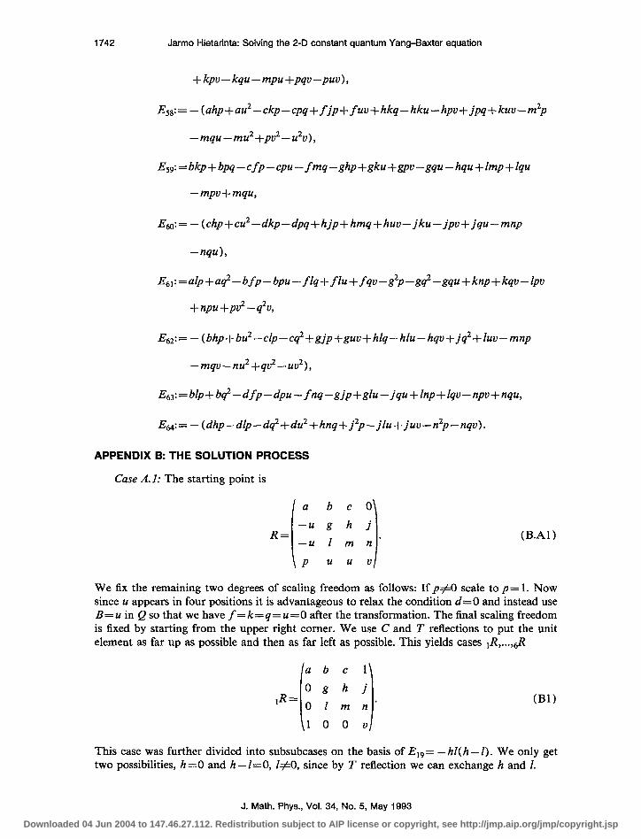
APPENDIX B: THE SOLUTION PROCESS

Case A.1: The starting point is

R=

p uuu

(B.Al)

We fix the remaining two degrees of scaling freedom as follows: If p#O scale to p= 1. Now since u appears in four positions it is advantageous to relax the condition d =0 and instead use B = u in Q so that we have f = k = q = u = 0 after the transformation. The final scaling freedom is fixed by starting from the upper right corner. We use C and T reflections to put the unit element as far up as possible and then as far left as possible. This yields cases lR,...,,$

This case was further divided into subsubcases on the basis of E,, = - hZ( h - I). We only get two possibilities, h=O and h-1=0, 1#0, since by T reflection we can exchange h and 1.




cu=Cd- Lf,h--I&- Lwl,

2R=

cz=Cb-- Mf,kp- l,q,uIt,

b2={{a-v,c-l,g+u,h-Z,j+1,Z2v+l,m+v,n+1}}.

3R=

c3=iIa- Lb,cd,f,j,kn,p- Lwl,

b3={~fl,h,Z,m+l,v-l},(g--l,h,l,m-l,v-1}, Cg-u,h-v-l,Z,m+l},

0 0 0 o\

0 1 h 0 4R= 0 I m 0’

1 0 0 o/

There are no solutions of this type. 0 0 0 0 0

SR=o 1 0 1 0 I 0 I 0’

1 0 0 0

c~=Cdw,d,f,g,h-- Lj,km,w- Lqwl,

032)

U33)

034)

W)

b,=CCO,CI- 111.



1

0 0 0 0 0 0 0 0

6R= 0 0 0 0’ 1 0 0 0 I

(I361

cg={a,b,c,d,f,g,h,j,k,I,m,n,p- l,q,u,v},

Next we have p=O and then u cannot be eliminated while keeping p=d= 0. First we assume that u is nonzero and scale to u = - 1 and start putting the other unit element from the . . diagonal, yleldmg 7R,...,ll R

lb CO

0 -1 -1 U

, (B7)

cl=Ca- Mf - Lk- l,p,q+ l,u+ l},

b7={{b+n,c+n,g+ l,h+2n,j-n,Z+2n,m+ l,u- l},{b+n,c+ng+ l,h,j-n,l,m+ l,v- 1)).

Ob CO

8R= 1 I mn 0 -1 -1 0

There are no solutions of this type.

Ob CO

0 -1 -1 0

038)

cg={a,d,f - l,g,h- l,k- l,m,p,q+ l,u+ l,u}, bg=CUw,jJ- Ln33. 01 co

1dz=

0 -1 -1 0

q~=Ca,b-- Mf - Lg,h,k- Lhp,q+ la+ Lvl,

039)

(BlO)

h=CCc- l,j+ l,n+ 133.



Jarmo Hietarinta: Solving the 2-D constant quantum Yang-Baxter equation

00 00 10 00

11R=

0 -1 -1 0

CII =Ca,b,c,d,f - Lg,hj,k-- 4Awvwt- l,u+ 4~3,

1745

0311)

Next we have p = 0, u = 0 in Eq. (B.A 1) and transform among b,c, j,n so that b = 1 for the subcases ,2R ,...,18R. (This can be done unless b=c=j=n=O, which is discussed later.) The other unit will be on the diagonal. Note that now C and T reflections are not allowed.

(J312)

This turned out to be computationally difficult, so we split it further into three parts using E,,= -1mh.

(1) I=0

~12.1 ={a- Lb- L4f,W,p,w3,

jv-m+n+v,m2-v,mn-m+n+v,mv+m+nv--n-2v,n2v-n2-4nv-v2+v},

{c+u,g+l,h-u-l,j,m-v,n},{c+l,g+h-l,j,m-l,n,v-1},

Cc&- l,j,m,w- 13,Cc,g,h,j,m-- Lw- l},Cc-- L&j,ww- 133.

It is often the case in computing Griibner bases that in a bad ordering of variables the result looks complicated. This holds for the first entry above, if we give up the default alphabetical ordering and instead put j and m last in the list of variables, then the first entry in b,,, splits into

Here the first solution is in fact the special case v=O of the second solution in b12,1 so it can be omitted.

(2) m=O, I#0

c12.2=(a- Lb- Wf,k,m,p,q,u3,

n12.2={{03, h=CCc+ Lg- M,jJ- hv- 133.

(3) h=O, m#O, I#0

c12.3=Ca- V- Mf,kbq,u3, n12,2=ICO,Cm33,



mv+m+nv2-nnv+2v,n2v2-n2V+4nV-V+ 1},

{cv+ l,g-v,j,Z--v- l,m+ l,n},{c+ l,g- l,j,Z+m- l,n,u- 1)).

Again a change in the variable ordering (j, n, m last in the list) produces a shorter result for the first element

13R= , (Bl3)

c13=Ca,b- Ld,f,kp,q,w- 13,

b~3=C{c,g,h,j- Ll- Lm,nh{c,g- Lh,jJ- Lm,n3,Cc-j,g+m- Lhjm-i+m,l,n- 13,

Cw- l,h,j,l,m- Ln33.

@=

c14=Ca,b- Mfe- lAp,qwh

b14={{c+ l,h+ l,j,Z,m,n3,{c+ Lh,j+ LZ,m+ M- 133.

cl~=Ca,b- Mf,g,km- Lp,q,w3,

h=CCc+ l,h,j,l+ 1~~33. h=CCc+ l,h,j,l+ 1~~33.

16R= 1 0 1 c 0

0 0 1 j

0 10

0 0 0 0 I n’ 16R=

m=Ca,b- Ld,f,g,h-- Lkwvww3,

(Bl4)

(J315)

(B16)

b16={{c- l,j-n,Z- 1)).




I+= , 0317)

c17=Ca,b-- Mf,g,hM- Lwww3,

b= CCcJ33.

1 0 1 c 0

0 0 0

NJ=

j

0 0 0 n’

0 0 0 0 I (J318)

ble={{cjn-cj+cn-jn}}.

Finally we havep=u=b=c=j=n=O in Eq. (B.Al) so we can only put one element to 1

19R=

Cgm+v,h,Z-v- 1),&h- l,Z- l,m,v},Cg,h- l,Z- l,m,v- 1)).

2oR=

c20= Ca,b,c,d,f ,g- Li,kn,p,q,w3,

21R =

~21 = Ca,b,w&f ,g,h - Lj,km,n,p,q,u,v3,

(Bl9)

G320)

0321)



b,,=CCO,CI- 133.

Case A.2: Now we have d= 0, f = k, g= m, q = u, and k + u#O, let us therefore scale so that k+u=l

R=

p uuv

(B.A2)

We start putting the other unit element from the lower left hand corner. Both C and T reflections are allowed, but may have to be accompanied with a redefinition of II.

In the first case we scale to p= 1 and have

W2)

Since u appears now in four places, we again give up the constraint d=O and instead transform with A=l, C=O, B=u in (Ml) to

(B22a)

(where the parameters have been redefined). Note that this transformation does not change the relations g= m, f = k, q= u. Now EM- Eh2 = hZ( h - I) so the problem splits into two, 1: h = I, 2: Z=O, h#O. There are no solutions in the second category, so let us concentrate on the first. With h = I we find E,, = b - c, E4, = j -n, thus the R matrix must have the nicely symmetric form

(B22b)

One property of the R matrix is that if it has b = c, j = n, f = k, q= u, g= m, h = I these relations will be preserved under a general Q transformation. To utilize this property, we try to transform 22$ to one of the forms studied before.

First we use the B part of Q to put d=O, yielding

a c c 0

l-u m I n 223 =

1 I

l-u I m n

1 uuv

(B22c)




(where the variables have been redefined, as usual). After the C part of Q we find

(f +~hv:= - (c+n)C2+(a-v)Ctl=O, (B22d)

pnew:=2(n-c)C3+(a-21-2m+v)C2+2(1--2u)C+l=O. (B22e)

A previously discussed subcase of Al is obtained if we can solve C from the first equation. If this cannot be done, we must have c = -n, a = v and if we then can solve for C from the second equation we again get a subcase of Al, after a reflection. The final exceptional case is n =c=O, a = u = I+ m, u = f, which yields

c22={a-Z-m,b,c,d,2f - l,g-m,h-Z,j,2k- l,n,p- 1,2q- 1,2u- Lv-Z-m},

622 = CU33,

as the only possibly new solution.

23R = (~23)

%={a- Mf +u- lg-m,k+u- l,p,q-u},

b23={{4b-v+ 1,4c-v+ l,h,4j+u2-v,Z,2m+v+1,4n+v2-v,uv-u-v},

{b-n,c-n,h,j-n,Z,2m-v-l,2u-l},~b,c,h+n,j-n,Z+n,m,u,v-1},

{b-Z,c-Z,h-Z,j,m+ l,n,u,uf 1},{4b-v2+ 1,4c-v2+ l,h,j,Z,2m-u-k l,n,u},

{b,c,h,4j+v2-l,Z,2m+v-l,4n+v2-l,u-l},{b,c,h+n,j-n,Z~n,m-l,u-l,v+1},

{b+Z,c+Z,h-Z,j,m,n,u-l,v-11)).



0 b c O\

l-u 24R=

i

1 h j l-u I 1 n ’

0 u u o/

There are no solutions of this type.

0 b c 0

25R = l-u 0 1 j ! I l-u I 0 n’

0 u u 0

c25=Ca,d,f +u- l,g,h- l,k+u- l,m,p,q-u,v},

b25= CCb,c,.i,l-- Ln33.

1 0 1 c 0

l-u 0 0

2&=

j l-u 0 0 n’

0 u u 0 I %={a,b- l,d,f +u- l,g,h,k+u-- Ll,m,p,q--u,v),

b26={{c- l,j- l,n- 1,2u- 1)).

0 0 0 o\ l-u 0 0 0

29 = ! l-u 0 0 0’ 0 u 210

~27=Ca,b,w&f +u- LgA,j,k+u- l,l,m,n,p,q-w),

b=CC33. Case BI: In the first B case the starting point is

R=

(B24)

(B25)

(B36)

(B27)

(B.Bl)

with q#u. If now b=c and p=O we can reflect the matrix to one of the forms studied before, thus we get two subcases: ( 1) b=c, p#O, and (2) b#c.

B 1.1 We fix the scaling freedoms by putting p = 1 and q = u + 2. We now have cE3 - 2acE4, + aE6 = 2c3 so in fact we must also take c = 0 and obtain



Jarmo Hietarinta: Solving the 2-D constant quantum Yang-Baxter equation

a 0 00

1751

(B28)

+a=Chc,d,f -kj,n,p- b-u-23,

{a+k+-v,g-k-v,h+k,k2 + + v k 2 ,I, m-v,u+l},{a-m,g+v,h-m-v,k,Z,mu+2m+uv},

{a-v,g+2u+v+2,h,k+u+1,Z+2u+2,m+v,u2+u-v},{a-Z+v,g-Z+v,h,k,Zu+2v,m+v},

{a,g,h,k,m,u,v},{a+u2+2u,g+u2+2u,h,k,Z,m+u2+2u,v}}.

B1.2 If b#c we may assume that one of them, say c, is nonzero and scale it to 1, thus we start with

29R= 1) (~29)

where b#l, q#u. For computational purposes it now turns out to be best to scale m to 1, if it is nonzero.

( 1) If m =0 we scale so that q-u = 2. For the simplest result we used a variable ordering that places I last in the list of variables.

c29.1={+ Mf -kj,ww--u-23,

{a-Z,b+ l,g+h-Z,hZ- l,k,p,u+ l,v-,},{a-v,b,g-v,hv--2,k,p,u+2,1}}.

(2) If m#O we scale to m = 1. This is a good illustration of the significance of variable ordering in computing Griibner bases. The default ordering produced a quite long output but when we finally found the best ordering (alphabetical, except that h, I last in the list) both the output and computation time was reduced almost by a factor of 10.

c29.2={+ Mf -kj,m- l,n),

n29,2=CCb- 13,Cq---33,

b29.2={{a+h,b,g+h- l,k+h,p+h2,q,u--k2,u+k- l,Z3,

{a-l- l,b+ l,g+h-Z- l,k,p,q-hZ,u+hZ,v-Z- l},




{a-h2+hZ+h+ l,b+h-Z- l,g+h-Z- l,k-h2+hZ+2h,

p-h3+h2Z+2h2,q-hl ,u+h3-h’l-2h2+hZ,v-h2+hZ+2h-Z-l},

Ca-v-h+Z+2,b+h-Z- l,g+h-Z- l,k-u+Z+ l,p+3-vZ-2v+Z+ 1,

q-v’+v-Z,u+vZ+v-l,vh-vl-vu-h+l}}.

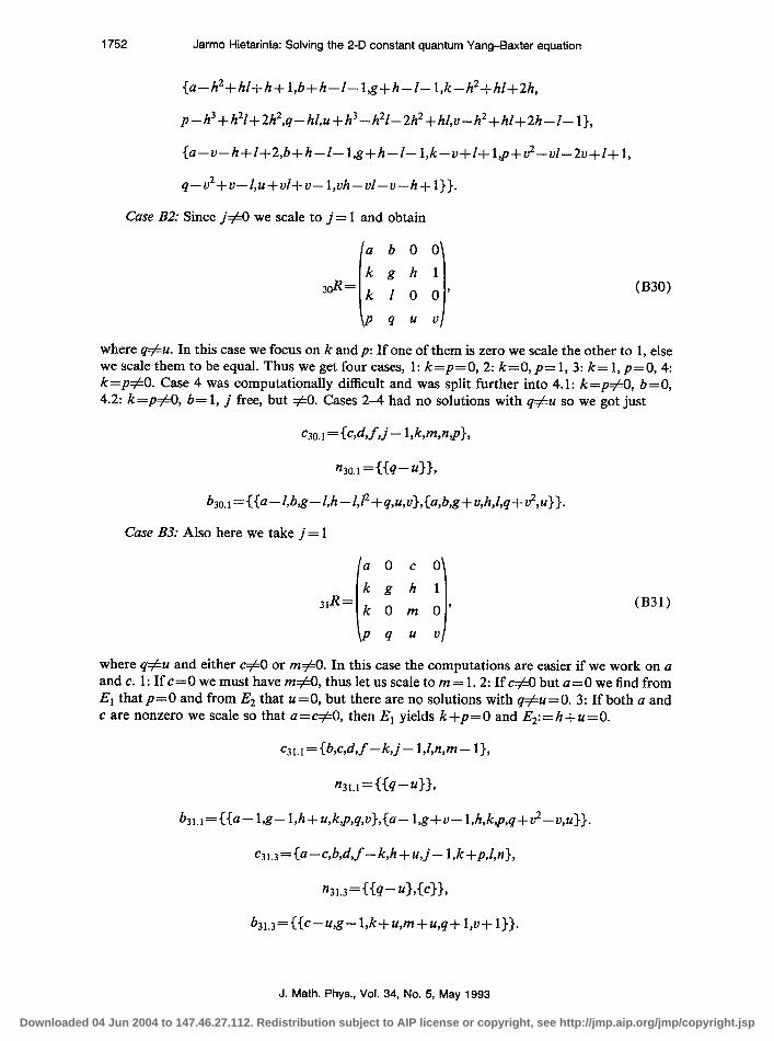
Case B2: Since j#O we scale to j= 1 and obtain

9 0330)

where q#u. In this case we focus on k and p: If one of them is zero we scale the other to 1, else we scale them to be equal. Thus we get four cases, 1: k=p=O, 2: k=O,p= 1, 3: k= 1, p=O, 4: k=p#O. Case 4 was computationally difficult and was split further into 4.1: k=p#O, b=O, 4.2: k=p#O, b= 1, j free, but #O. Cases 2-4 had no solutions with q#u so we got just

~30.1 =Cc,d,f,j-- Lkmw3,

n30.1= CCq- 43,

Case B3: Also here we take j= 1

31R= (I3311

where q#u and either c#O or m#O. In this case the computations are easier if we work on a and c. 1: If c = 0 we must have m#O, thus let us scale to m = 1.2: If c#O but a = 0 we find from El that p=O and from E2 that u =0, but there are no solutions with qfu = 0. 3: If both a and c are nonzero we scale so that a = c#O, then E, yields k +p = 0 and E2: = h + u = 0.

w1=Cb,c,d,f -k-i- LAn,m- 13,

b31.1={Ca- Lg- Lh+u,kp,q,~3,Ca-- kg+- Lh,kp,q+~-w33.

c31.3=Ca-c,W,f -M+u,j- l,k+p,Z,n3,

b31.3=CCc-u,g- l,k+u,m+u,q+ l,v+ 133.




Case C This is the special case

a c c 0

R=

P 4 u v

(B.C)

with f#k, q#u, p#O, we will therefore scale to p= 1. Now E3=c2(f -k+q-u) and E48 =n2(f-k+q-u) so we must either have c=n=O or f-k+q-u=O. In the first case we have

32R= (B32)

with f#k, q#u and scale to get two subcases, 1: k=O, f = 1, q#u, 2: k= 1, f#l, q#u. (In the second subcase we may also assume that f#O otherwise the solution would be obtained from the first by T reflection.)

&.I= CCa- vJ,m - v,q,u - 13,Ca,l,m,q,v3,Ca,l,m,u,v)).

c32.2=Cb,c,dtg-m,h-Z,j,k- l,n,p- 13,

n32.2=CCq-u3,Cf - 13,Cf33,

b32.2=CCa--v,f + l,Z,m--,q+v,u--},{a--,f -u,Z,m--,q- 13,

(a,fqu+fq-fu-qu,m,Z,v33.

In the last case we can scale so that f = k+ 1 and then q= u - 1

k+l m I n 33R = k I mn (B33)

and we may also assume that n#O or c#O, else we get back to 32R. From E32 + Es6 = n (c - 3n) and E2 + E3=c(3c-n) we see that there are no solutions of this type.



APPENDIX C: ANALYSIS AT THE RAW DATA

TABLE I. Analysis of the raw data. “Case” refers to subscripts of c and b Appendix B. The canonical homogeneous form to which a solution can be transformed is given in column 3.

Case Subcase Transforms to R,,,

1.1 1

1.2 1 2

2

3

5

6

7

9

10

11

12.1

12.2

12.3

13

1

1 2 3 4 5 6

1 2

1

1 2

1

1

1

1 2 3 4 5 6 1 8

1

1 2 3

1 2 3 4

14 1 2

15 1

1.4

0.2 n2= (P- 1)2/4Z, 3P+ l#O: 0.2,

n2=(Zr-1)2/4Z, 3P+l=O: 1.6, else 1.4 m+u=O: 1.4, else 1.1

3.1 see # 3 above

3.1

Z’=4: 0.1, else 1.4

0.1 2.3 1.2 1.2 1.2 1.2

1.8 1.4

2.3

n=O,l: 0.1, else 1.4 n=O: 0.1, else 1.4

1.6

1.4

1.6

2.2 1.2

h=O: 1.3, else 2.1 0.1

c#Q m= 1 or c=O, u= 1: 2.3, else 3.1 0.4 1.5 0.6

2.1

2.2 1.2

m=l: 1.3, else 2.1

2.2 1.2 3.1 1.5

1.12 3.1

1.12




TABLE I. (Continued. )

case 16

Subcase

1

Transforms to R,. ~

1.6

17 1 1.8

18 1 see Sec. V B 1

19 1 3.1 2 2.1 3 2.2 4 5

2.1 2.2

6 0.5 7 0.3

20

21 1 1.12 2 1.4

22 1 2.3

23 1 1.6 2 n= -(m- 1)‘/2: 2.3, else 3.1 3 n=O: 0.6, n=l: 1.2, else 1.1 4 l=O: 1.2, I= - 1: 0.6, else 1.1 5 u=O: 1.6, else # 4 above 6 # 4 above 7 # 4 above 8 # 3 above

25 1 1.6

26 1 3.1

27 1 1.6

28 U=-1: 1.7, u=-2: 1.12, else 2.1 k=O: 1.7, else 2.2

m+ufO: 1.2 m+u=O, u=-1: 1.7, else 1.11 1.8

m+u=O: 1.7, else 1.2 u=-1: 1.7, u=O: 1.12, else 2.1

see # 3 above 1.8

1 1.12 2 3.1 3 1.12

u=-2,O: 1.11, else 1.5

29.1 1.2 1.2

P+ 1 =O: 1.3 else 2.1 1.5

29.2 h=l: 1.11 else 1.5 h=-Z=l: 1.11, h=-Z#l: 1.3, h#-/cl: 1.12, else 2.1

h=l: 1.11, else 1.2 u=O: 1.11, else 1.2



TABLE I. (Continued. )

Case Subcase Transforms to R, B

30.1 1 0.4 2 1.8

31.1 1 2

31.3 1 1.8

32.1 1 2.3 2 u= 1: 2.3, else 1.9 3 q=l: 1.7, else 1.10

32.2 1 1.3 2 2.3 3 seeSec.VB 1

1.5 1.5

‘R. J. Baxter, Exactly Solved Models in Statistical Mechanics (Academic, New York, 1982). ‘P. P. Kulish and E. K. Sklyanin, in Integrable Quantum Field Theories, edited by J. Hietarinta and C. Montonen

(Springer, New York, 1982), pp. 61-119; L. Faddeev, in Integrable systems, Nankai lectures 1987, edited by M.-L. Ge and X. C. Song (World Scientific, Singapore, 1989), pp. 23-70; E. K. Sklyanin, Preprint HU-TFTdl-51 (1991).

‘L. A. Takhtajan, in Introduction to Quantum Group and Integrable Massive Models of Quantum Field Theoty, edited by M.-L. Ge and B.-H. Zhao (World Scientific, Singapore, 1990), pp. 69-197.

‘Braid Group, Knot Theory, and Statistical Mechanics, edited by C. N. Yang and M. L. Ge (World Scientific, Singapore, 1989).

‘M. Jimbo, Introduction to the Yang-Baxter Equation, in Ref. 4; Yang-Baxter Equation in Integrable Systems, edited by M. Jimbo (World Scientific, Singapore, 1990).

6K. Sogo, M. Uchinami, Y. Akutsu, and M. Wadati, Prog. Theor. Phys. 68, 508 (1982). ‘L. Hlavaty, J. Phys. A 20, 1661 (1987). ‘P. P. Kulish and E. K. Sklyanin, J. Sov. Math. 19, 1596 (1982). 9M. Jimbo, Commun. Math. Phys. 102, 537 (1987); V. V. Baxhanov, ibid. 113, 471 (1987).

“J. Hietarinta, Phys. Lett. A 165, 245 (1992). “J H Davenport, Looking at a set of equations, Bath Computer Science Technical Report 87-06; H. Melenk, CWI . .

Quarterly 3, 121 (1990). I2 H. Melenk, H. M. Moller, and W. Neun, GROEBNER, A Package for Calculating Groebner Bases (Included in the

REDUCE 3.4 distribution package.) 13A. C. Hearn, REDUCE User’s Manual Version 3.4, CP 78 (Rand, Santa Monica, 7/91). “S.-M. Fei, H.-Y. Guo, and H. Shi, J. Phys. A 25, 2711 (1992); and S.-M. Fei (private communication). “L. Hlavaty, J. Phys. A 25, L63 (1992).



Jarmo Hietarinta : Solving the two-dimensional constant quantum ...

Documents

Transcript of Jarmo Hietarinta : Solving the two-dimensional constant quantum ...