January 21, 2007 - SRON

Observational Astrophysics I

JOHAN BLEEKERSRON Netherlands Institute for Space Research

Astronomical Institute Utrecht

January 21, 2007

Contents

1 Discovery Space 41.1 Historical remarks . . . . . . . . . . . . . . . . . . . . . . . . . . . . . . . . . . 41.2 Discovery and rediscovery . . . . . . . . . . . . . . . . . . . . . . . . . . . . . . 51.3 The search . . . . . . . . . . . . . . . . . . . . . . . . . . . . . . . . . . . . . . 71.4 The phase space of observations . . . . . . . . . . . . . . . . . . . . . . . . . . . 101.5 Estimating the total number of cosmic phenomena . . . . . . . . . . . . . . . . 111.6 Unimodal and Multimodal Phenomena . . . . . . . . . . . . . . . . . . . . . . . 121.7 The End of the Search . . . . . . . . . . . . . . . . . . . . . . . . . . . . . . . . 13

2 Information Carriers 152.1 Electromagnetic radiation . . . . . . . . . . . . . . . . . . . . . . . . . . . . . . 15

2.1.1 Characterisation . . . . . . . . . . . . . . . . . . . . . . . . . . . . . . . 152.1.2 Thermal radiation . . . . . . . . . . . . . . . . . . . . . . . . . . . . . . 162.1.3 Non-thermal radiation . . . . . . . . . . . . . . . . . . . . . . . . . . . . 192.1.4 Astrophysical relevance . . . . . . . . . . . . . . . . . . . . . . . . . . . 242.1.5 Multispectral correlations . . . . . . . . . . . . . . . . . . . . . . . . . . 262.1.6 Observing locations . . . . . . . . . . . . . . . . . . . . . . . . . . . . . 27

2.2 Neutrinos . . . . . . . . . . . . . . . . . . . . . . . . . . . . . . . . . . . . . . . 292.2.1 Characterisation . . . . . . . . . . . . . . . . . . . . . . . . . . . . . . . 292.2.2 Astrophysical relevance . . . . . . . . . . . . . . . . . . . . . . . . . . . 302.2.3 Observing locations . . . . . . . . . . . . . . . . . . . . . . . . . . . . . 30

2.3 Cosmic-rays . . . . . . . . . . . . . . . . . . . . . . . . . . . . . . . . . . . . . . 302.3.1 Characterisation . . . . . . . . . . . . . . . . . . . . . . . . . . . . . . . 302.3.2 Astrophysical relevance . . . . . . . . . . . . . . . . . . . . . . . . . . . 312.3.3 Observing locations . . . . . . . . . . . . . . . . . . . . . . . . . . . . . 31

2.4 Gravitational radiation . . . . . . . . . . . . . . . . . . . . . . . . . . . . . . . . 312.4.1 Characterisation . . . . . . . . . . . . . . . . . . . . . . . . . . . . . . . 312.4.2 Astrophysical relevance . . . . . . . . . . . . . . . . . . . . . . . . . . . 332.4.3 Observing locations . . . . . . . . . . . . . . . . . . . . . . . . . . . . . 33

3 Stochastic Character of Radiation Fields 343.1 Radiometric units . . . . . . . . . . . . . . . . . . . . . . . . . . . . . . . . . . . 343.2 Random phenomena and variables . . . . . . . . . . . . . . . . . . . . . . . . . 35

3.2.1 Parent population . . . . . . . . . . . . . . . . . . . . . . . . . . . . . . 353.2.2 Discrete and continuous distributions: expectation values . . . . . . . . 373.2.3 Sample parameters . . . . . . . . . . . . . . . . . . . . . . . . . . . . . . 38

3.3 Probability density distributions . . . . . . . . . . . . . . . . . . . . . . . . . . 393.3.1 The binomial and Poisson distributions . . . . . . . . . . . . . . . . . . 39

1

3.3.2 The Normal or Gaussian distribution . . . . . . . . . . . . . . . . . . . . 413.3.3 The Lorentzian distribution . . . . . . . . . . . . . . . . . . . . . . . . . 42

3.4 Method of maximum likelihood . . . . . . . . . . . . . . . . . . . . . . . . . . . 433.4.1 Calculation of the mean . . . . . . . . . . . . . . . . . . . . . . . . . . . 433.4.2 Estimated error of the mean . . . . . . . . . . . . . . . . . . . . . . . . 45

3.5 Stochastic processes . . . . . . . . . . . . . . . . . . . . . . . . . . . . . . . . . 453.5.1 Distribution functions . . . . . . . . . . . . . . . . . . . . . . . . . . . . 453.5.2 Mean and variance . . . . . . . . . . . . . . . . . . . . . . . . . . . . . . 46

3.6 Intrinsic stochastic nature of a radiation beam . . . . . . . . . . . . . . . . . . 463.6.1 Bose-Einstein statistics . . . . . . . . . . . . . . . . . . . . . . . . . . . 463.6.2 Electromagnetic radiation in the thermal limit . . . . . . . . . . . . . . 483.6.3 Electromagnetic radiation in the quantum limit . . . . . . . . . . . . . . 51

4 Physical principles of radiation detction 534.1 Types of detection . . . . . . . . . . . . . . . . . . . . . . . . . . . . . . . . . . 53

4.1.1 Amplitude detection . . . . . . . . . . . . . . . . . . . . . . . . . . . . . 534.1.2 Power (or intensity) detection . . . . . . . . . . . . . . . . . . . . . . . . 53

4.2 Detection of electromagnetic radiation . . . . . . . . . . . . . . . . . . . . . . . 544.2.1 Opacity, cross-section, Kirchhoff’s law . . . . . . . . . . . . . . . . . . . 544.2.2 Thermal detection . . . . . . . . . . . . . . . . . . . . . . . . . . . . . . 554.2.3 Photo-electric detection . . . . . . . . . . . . . . . . . . . . . . . . . . . 56

4.3 Neutrino detection . . . . . . . . . . . . . . . . . . . . . . . . . . . . . . . . . . 664.4 Cosmic-ray detection . . . . . . . . . . . . . . . . . . . . . . . . . . . . . . . . . 69

5 Characterization of instrumental response 725.1 Characteristic parameters . . . . . . . . . . . . . . . . . . . . . . . . . . . . . . 72

5.1.1 Bandwidth (symbol: λλ, νν, or εε) . . . . . . . . . . . . . . . . . . . . . 725.1.2 Field of view (FOV, symbol: ΩFOV ) . . . . . . . . . . . . . . . . . . . . . 725.1.3 Precision and resolution . . . . . . . . . . . . . . . . . . . . . . . . . . . 735.1.4 Limiting sensitivity [symbol: (F (λ, ν, ε)min] . . . . . . . . . . . . . . . . 765.1.5 Polarisation sensitivity (symbol: Πmin) . . . . . . . . . . . . . . . . . . . 76

5.2 Convolutions . . . . . . . . . . . . . . . . . . . . . . . . . . . . . . . . . . . . . 785.2.1 General . . . . . . . . . . . . . . . . . . . . . . . . . . . . . . . . . . . . 785.2.2 Fourier transforms . . . . . . . . . . . . . . . . . . . . . . . . . . . . . . 80

5.3 Instrument response and data sampling . . . . . . . . . . . . . . . . . . . . . . 815.3.1 Response fuctions . . . . . . . . . . . . . . . . . . . . . . . . . . . . . . 815.3.2 Discrete measurement intervals, the Nyquist criterion . . . . . . . . . . 835.3.3 Noise . . . . . . . . . . . . . . . . . . . . . . . . . . . . . . . . . . . . . 84

5.4 The Central Limit Theorem . . . . . . . . . . . . . . . . . . . . . . . . . . . . . 86

6 Signal to Noise Ratio 886.1 General . . . . . . . . . . . . . . . . . . . . . . . . . . . . . . . . . . . . . . . . 886.2 Temperature characterisation . . . . . . . . . . . . . . . . . . . . . . . . . . . . 89

6.2.1 Brightness and antenna temperature . . . . . . . . . . . . . . . . . . . . 896.2.2 Noise sources at radio wavelengths . . . . . . . . . . . . . . . . . . . . . 906.2.3 The SNR-degradation factor . . . . . . . . . . . . . . . . . . . . . . . . 93

6.3 Power characterisation . . . . . . . . . . . . . . . . . . . . . . . . . . . . . . . . 946.3.1 Typical set-up of observation . . . . . . . . . . . . . . . . . . . . . . . . 946.3.2 Responsivity . . . . . . . . . . . . . . . . . . . . . . . . . . . . . . . . . 95

6.3.3 The Noise Equivalent Power (NEP) . . . . . . . . . . . . . . . . . . . . 966.4 Quantum characterisation . . . . . . . . . . . . . . . . . . . . . . . . . . . . . . 97

7 Imaging in Astronomy 1007.1 Diffraction . . . . . . . . . . . . . . . . . . . . . . . . . . . . . . . . . . . . . . . 101

7.1.1 The Huygens-Fresnel principle . . . . . . . . . . . . . . . . . . . . . . . 1017.1.2 Fresnel and Fraunhofer diffraction . . . . . . . . . . . . . . . . . . . . . 1017.1.3 Point Spread Function (PSF) and Optical Tranfer Function (OTF) in

the Fraunhofer limit . . . . . . . . . . . . . . . . . . . . . . . . . . . . . 1027.1.4 Circular pupils . . . . . . . . . . . . . . . . . . . . . . . . . . . . . . . . 1077.1.5 Rayleigh Resolution Criterion . . . . . . . . . . . . . . . . . . . . . . . . 1107.1.6 Complex pupils . . . . . . . . . . . . . . . . . . . . . . . . . . . . . . . . 110

7.2 Other limits to image quality . . . . . . . . . . . . . . . . . . . . . . . . . . . . 1117.2.1 Optical aberrations . . . . . . . . . . . . . . . . . . . . . . . . . . . . . . 1117.2.2 Atmospheric degradation: speckle images . . . . . . . . . . . . . . . . . 1137.2.3 Seeing: the Fried parameter . . . . . . . . . . . . . . . . . . . . . . . . . 1167.2.4 Real time correction: principle of adaptive optics . . . . . . . . . . . . . 118

7.3 High energy imaging . . . . . . . . . . . . . . . . . . . . . . . . . . . . . . . . . 1207.3.1 Grazing incidence telescopes . . . . . . . . . . . . . . . . . . . . . . . . . 1207.3.2 Non-focussing optics: beam modulation . . . . . . . . . . . . . . . . . . 1237.3.3 Gamma-ray imaging . . . . . . . . . . . . . . . . . . . . . . . . . . . . . 126

8 Spectroscopy in Astronomy 1348.1 Spectral diagnostics in Astrophysics . . . . . . . . . . . . . . . . . . . . . . . . 134

8.1.1 Physical source parameters embedded in spectral information . . . . . . 1348.1.2 Continuum and line emission . . . . . . . . . . . . . . . . . . . . . . . . 1348.1.3 Characterisation of spectral lines . . . . . . . . . . . . . . . . . . . . . . 134

8.2 Spectral separation principles . . . . . . . . . . . . . . . . . . . . . . . . . . . . 1348.2.1 General concepts . . . . . . . . . . . . . . . . . . . . . . . . . . . . . . . 1348.2.2 Interferometric separation techniques . . . . . . . . . . . . . . . . . . . . 1348.2.3 Non-interferometric separation techniques . . . . . . . . . . . . . . . . . 134

Chapter 1

Discovery Space

1.1 Historical remarks

Traditional astronomy was concerned with studying the light, i.e. optical radiation,from ob-jects in space. The range of light is in fact surprisingly limited, it includes only radiation withwavelenghts 30 percent shorter to 30 percent longer than the wavelength to which the humaneye is most sensitive. Present day astronomy covers the full electromagnetic spectrum cov-ering wavelenghts less than one thousand-millionth as long (gamma-rays), to over a hundredmillion times the wavelength of light for the longest radio waves. To make an analog withsound, traditional astronomy was an effort to understand the symphony of the universe withears which could hear only middle C and the two notes immediately adjacent.The accidental discovery in 1931 by Karl Jansky, a radio engineer at Bell Telephone Labora-tory, of radio waves beyond the Earth showed that there was non-optical radiations from space.The rapid growth of astronomy over the recent decades basically arises from overcoming twomajor barriers.

The first is a natural barrier, the earth’s atmosphere, which absorbs most radiations fromspace,consequently space-based instruments and platforms are required to cross this barrier.This ”space age” started in the 1950s and has been absolutely seminal for the developmentof modern astrophysics.

The second barrier was technological: new types of telescopes had to be built to gatherother kinds of electromagnetic radiation than optical or radio waves, this also included tech-niques for collecting cosmic-ray particles and neutrinos. Also, a host of new sensor techniquesto detect and record the images and spectra gathered by these telecopes needed to be devel-oped, including their suitability to be launched by rockets and carried on satellite platformsoperated in space. As a consequence, many cosmic phenomena have only come to be recog-nized in the past forty-five years, largely through the introduction into astronomy of radio,X-ray, infrared, and gamma-ray techniques. None of the new phenomena had been antici-pated before World War II, and it is natural to wonder how many more remain unrecognizedeven today, how rich and complex the universe might be. Further, if technological advancesalready have helped us uncover so many new cosmic features, how many more innovations ofsimilar kinds could we put to use in future cosmic searches?

Astronomy is largely an observational science, and for at least the next century our tech-nology will be insufflciently advanced to permit exploration of the universe beyond the solarsystem. Because astronomy is so dependent on observations, it is relatively simple to assessthe impact that further technological advances are likely to make. In the experimental sci-ences such an assessment would be far more complex. The experimentalist studies a system

4

Figure 1.1: Observation, experiments, and exploration. Observation is the most passive meansfor gathering data. The observer receives and analyzes information transmitted naturally bythe system he is studying. The experimenter, in contrast, stimulates the system under con-trolled conditions to evoke responses in some observable fashion. Exploration is an attempt togather increasing amounts of information by means of a voyage which brings the experimenteror observer closer to the system to be studied.

by imposing constraints and observing the system’s response to a controlled stimulus. Thevariety of these constraints and of stimuli may be extended at will, and experiments can be-come arbitrarily complex as indicated in figure 1.1.Astronomy is different. The observer has only two choices. He can seek to detect and an-

alyze signals incident from the sky, or he may choose to ignore them. But he has no way ofstimulating a cosmic source to alter its emission. He can only observe what is offered. He isentirely dependent on the carriers of information that transmit to him all he may learn aboutthe universe.

1.2 Discovery and rediscovery

Though there is no unique definition of a cosmic phenomenon, most astronomers would com-pile a list much like the one shown in figure 1.2 if asked to name the principal phenomenacharacterizing the universe.The 43 phenomena named are given prominence in most astronomical texts and standard

reference works. Conferences and symposia concern themselves with individual phenomenaon the list, and books or review articles frequently focus on one or another of these entries.The discovery dates for the phenomena shown in the top curve cannot always be precisely pin-pointed because the realization of a discovery sometimes dawns slowly. At times a discoveryinvolves the recognition that a previously known phenomenon actually comprises two quitedistinct sources or classes of events — giant and main sequence stars, novae and supernovae,galaxies that contain gas — while others do not. Such discoveries are indicated by a slash (/)in the designation of the two phenomena that become resolved. The lower curve shows phe-

5

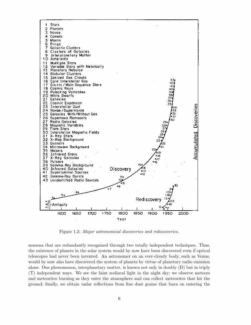
Figure 1.2: Major astronomical discoveries and rediscoveries.

nomena that are redundantly recognized through two totally independent techniques. Thus,the existence of planets in the solar system would by now have been discovered even if opticaltelescopes had never been invented. An astronomer on an ever-cloudy body, such as Venus,would by now also have discovered the system of planets by virtue of planetary radio emissionalone. One phenomenon, interplanetary matter, is known not only in doubly (D) but in triply(T) independent ways. We see the faint zodiacal light in the night sky; we observe meteorsand meteorites burning as they enter the atmosphere and can collect meteorites that hit theground; finally, we obtain radar reflections from fine dust grains that burn on entering the

6

upper atmosphere.The most striking aspect of the two curves is the increasingly accelerated rate of discoveryshown by the rapid rise in the top curve. Simultaneously with this rise comes an increasingrecognition of previously known phenomena, now rediscovered by means of radio telescopes.

1.3 The search

The search for cosmic phenomena is one of mankind’s greatest adventures and one of the mostambitious enterprises of modern science. To understand its conduct we will need to discern thenature of the phenomena, identify the people caught up in the search, describe the skills thesescientists possess, analyze the plans they follow to their goals, and identify the tools requiredfor their quest. We will need to know how the most significant discoveries are being made,whether past successes can guide us to further discoveries, whether there are ways to gaugethe future scope of the search — of deciding whether our inventory of cosmic phenomena isnearly complete, whether we are close to being the last generation of astronomers needed tounravel the complexities of the universe, or whether there will be an endless cadre of cosmicresearchers stretching into an uncertain future. There is only one way to approach this study:we must look at the conduct of past searches in order to discern trends that can lead toassessments of the future. Seven traits common to many discoveries are these:

1. The most important observational discoveries result from substantial tech-nological innovation in observational astronomy.Galileo’s spyglass enabled him to resolve features on the moon considerably finer thanany that can be distinguished with the unaided eye. He could also see stars severalmagnitudes fainter. Viktor Hess’s discovery of cosmic rays led to an increasing aware-ness that electromagnetic radiation is not the only carrier of astronomical informationreaching Earth; there also exist energetic subatomic particles that inform us about catas-trophic events far away in the cosmos. Karl Jansky looked out into the universe and sawsignals from our galaxy at wavelengths 20 million times longer than anything the eyecan see; the scientists at the Naval Research Laboratory and at the American Scienceand Engineering Corporation were able to detect signals at wavelengths 1,000 timesshorter than visible light, and these techniques led to the discovery of X-ray stars andgalaxies. The Vela military satellites could detect brief bursts of gamma-rays and foundjust such bursts arriving from unknown parts in the sky; and short pulses detected atradio wavelengths similarly had led Anthony Hewish and Jocelyn Bell to the discoveryof pulsars in 1968. Technological innovations that led to discovery have usually involvedcompletely new wavelength ranges never used in astronomy before, or have made useof instruments with unprecedented precision for resolving sources to exhibit structuralfeatures, time variations or spectral features never seen before.

2. Once a powerful new technique is applied in astronomy, the most profounddiscoveries follow with little delay.Many discoveries are made within weeks or months of the introduction of new observingequipment. In the past twenty-five years there have been no discoveries that couldhave been made with instruments available a quarter-century earlier. Occasionally adiscovery is verified by an observer who can point to records he had obtained some twoor three years before; on these the new phenomenon may already be discerned, thoughnot perhaps convincingly enough to stand out.

7

3. A novel instrument soon exhausts its capacity for discovery.This corollary to the speed with which new discoveries follow technical innovations doesnot imply that new apparatus quickly becomes useless. It just means that the instru-ment’s function changes. It joins an existing array of tools available to the astronomerfor analytical work, rather than for discovery, and continues useful service in that ca-pacity. To revitalize a technique for further searches for new phenomena, its sensitivityor resolving power must be substantially increased, often by as much as several fac-tors of 10. Thus the discovery of quasars became possible only after radio-astronomicaltechniques had advanced to a stage at which sources subtending angles no larger than 1second of arc could be identified and accurately located in the sky. The radio equipmentavailable earlier to Jansky could simply not have coped with such observations.

4. New cosmic phenomena frequently are discovered by physicists and engineersor by other researchers originally trained outside astronomy.In a wide-ranging study of the emergence of radio astronomy in Great Britain, thesociologists David Edge and Michael Mulkay have noted that all of the early British radioastronomers were physicists or electrical engineers and that radio astronomy, worldwide,was originally staffled largely by workers trained in physics or electrical engineering.The same trait can be discerned all across modern astronomy. We speak of ”cosmic-ray physicists”, and, in fact, cosmic-ray research is largely carried out in the physicsdepartments of universities. Similarly, the early X-ray or gamma-ray astronomers hadbeen trained as physicists. This trend is not just confined to modern times. We needonly think of the work of Galileo, William Herschel and Joseph Fraunhofer, who broughtnew methods and techniques to astronomy after working in other fields. Many of thesepioneers initially worked at what professional astronomers would have considered theoutskirts of astronomy.

5. Many of the discoveries of new phenomena involved use of equipment origi-nally designed for military use.The rapid development of radio astronomy after World War II was made possible byexisting radar equipment developed for the war effort. Even before the war’s end, how-ever, James Stanley Hey, at the time employed by the British radar network, had notedoccasional strong radio emission from the Sun and had discovered radar reflections frommeteor trails. Subsequently both solar radio astronomy and radar meteor observationsdeveloped into subdisciplines with their own practitioners. In 1946, shortly after theend of the war, Hey and his collaborators, still using war-time equipment available tothem, also discovered a curiously undulating cosmic radio signal that proved to be thefirst extragalactic radio source, Cygnus A. In the United States the earliest post-warsolar X-ray and far-ultraviolet observations were carried out with German V-2 rockets.Advances in infrared astronomy were similarly based on progress in the construction ofmilitary detectors, but the most sensitive far-infrared detectors were not developed untilsome time after the war and did not become available for astronomical work until thelate 1950s and early 1960s. This relationship between the tools of surveillance in warand in astronomy is not new: Galileo had pointed out the military value of the spyglassto the Venetian senate. His gift of the spyglass so pleased the senators that they atonce doubled his salary and made his professorship at the University of Padua a lifetimeappointment.

6. The instruments used in the discovery of new phenomena often have beenconstructed by the observer and used exclusively by him.

8

The instruments used by Galileo, Hess, Jansky, and the early X-ray astronomers werebuilt by them and were under their sole control. The Los Alamos group that discov-ered gamma-ray bursts had access to all the data gathered by the passive Vela satellites.Men like Christian Huygens, James Bradley, William Herschel, Friedrich Wilhelm Bessel,William Huggins, and William Parsons, third earl of Rosse, responsible for prime discov-eries in the seventeenth, eighteenth and nineteenth centuries, also had instruments thatthey alone might use: When faced with a surprising result, they could check their ap-paratus at leisure, repeat the observations, and cross-check their results until they werecertain that a finding was genuine and not due to some instrumental artifact. Morethan half of the phenomena discovered in historical times were made with instrumentsunder exclusive control of the astronomers responsible for the discovery.

7. Observational discoveries of new phenomena frequently occur by chance —they combine a measure of luck with the will to pursue and understand anunexpected finding.Before Viktor Hess set out to make his balloon observations, the slow discharge thatalways takes place in electroscopes had generally been attributed to radioactivity in theearth. If that were true, Hess argued, absorption of the radiation in 5 kilometers ofair should shield his instruments and cause them to discharge more slowly. Instead,Hess noted an increased discharging rate at higher altitudes and concluded that therays were cosmic. Karl Jansky, in 1931, was concerned with the mundane problem offinding ways to lower interference in radio telephone transmission. Instead he is nowremembered for finding radio emission from the Milky Way. The Los Alamos gamma-ray physicists were searching for surreptitious nuclear bomb tests and found cosmicgamma-ray bursts instead. The first X-ray star was discovered through a search forlunar X-ray fluorescence. The cosmic microwave background radiation was found whenArno Penzias and Robert Wilson at Bell Laboratories found they could not reduce belowa certain level the noise registered by a new sensitive radiometer they had developed.Pulsars forced attention upon themselves when Anthony Hewish and Jocelyn Bell wereactually set to measure scintillation — twinkling — of radio sources. About half thecosmic phenomena now known were chance discoveries. The number of these surprisesis a measure of how little we know our universe.

In addition to providing new discoveries, novel astronomical techniques have also providedanother, almost equally important datum, the rediscovery of phenomena recognized fromearlier observations. Frequently even this rediscovery occurs unexpectedly. The detectionof strong radio emission from Jupiter in 1955 represented the first, unexpected measure ofradio emission from a planet. Previously, planets had been considered to be undetectablewith available radiotelescopes because their theoretically predicted flux was too low to permitdetection.We say that a phenomenon is recognized in two completely independent ways if itcould be discovered equally well with separate instruments that differ by at least a factor ofa 1000 in one of their observing capacities. Spiral galaxies, for example, can be recognizedequally well through radio observations and through optical studies at wavelengths a milliontimes shorter. This independent recognition of phenomena through widely differing channelsof information provides a statistical key to the total number of observational discoveries wemight ultimately hope to make. A simple example illustrates the idea: consider a collection ofbaseball or football cards. At the beginning of each season when the collection is still small,all the cards differ from each other. But as the collection grows, an increasingly large fractionof the cards becomes duplicated. Assume that all individual pictures are equally represented

9

Figure 1.3: Phase space of discoveries.

and assume further that the cards are obtained in some statistically random order. Then thevery first duplicate obtained tells us an important characteristic of the set — namely,that it isfinite. In a collection containing an infinite number of different cards randomly distributed,no duplicates would ever be found unless an infinite number of cards were examined. As thecollection of cards grows and the number of duplicates increases, the relationship between thenumber of single cards in the collection and the number of duplicates can yield an increasinglyaccurate estimate of the total number of different cards in a complete set. The statisticsgoverning our search for cosmic phenomena through different channels of observation is similarto the statistics of baseball cards. Each newly opened channel corresponds to a newly openedpackage of cards. Initially, as our technical expertise grows and the number of availablechannels increases, we discover an increasing number of new phenomena. But as the numberof our discoveries grows, a survey carried out through a completely new channel will mainlyuncover an increasing number of duplicates, i.e. phenomena already known from earlierdiscovery through previously established channels. We currently recognize already quite anumber of duplicates, the rediscoveries of figure 1.2, such as the planets and the spiral, gas-containing galaxies.Thus the number of cosmic phenomena is finite and can be estimated!

1.4 The phase space of observations

The phase space of observations is a multidimensional space, each point of which correspondsto a different basic observing capability. The rectangular bordershown in figure 1.3 encom-passes the space containing all conceivable astronomical observations that can be carried outin our universe. The region of this space in which a given phenomenon appears, are deter-mined by its observable traits and not by its position in the sky. The phenomenon’s locationin the phase space will therefore not change appreciably from one phase in the evolution of ourgalaxy to the next, though the constellations of stars seen in the sky would change appreciablyduring that time. If we consider the case of electromagnetic observations, as an example, fiveorthogonal axes can be defined, i.e. the spectral frequency or wavelength of the observation,the angular resolution, the time resolution and the polarization of the received light. Theparameters define a five-dimensional space and any point contained in this space correspondsto a particular observation one can carry out. Conversely, any observation one might pos-sibly conceive corresponds to one or more points that can be unambiguously located in thevolume. This five-dimensional space constitutes therefore the phase space for electromagneticobservations (sometimes a sixth dimension, the intensity, is also added to EM-phase space).

10

The framed portion of figure 1.3 represents the entire accessible multidimensional space.The shaded portions are regions in which observations have already been undertaken. Thecosmic phenomena are represented by a variety of symbols. Some of these symbols appearin several portions of the space. Violins appear both in a region to which we already haveaccess and in a portion of the space in which we currently lack the instrumental capabilitiesto observe. Some phenomena, such as the one represented by the Greek letter Φ appearonly once. Some, like the question marks or the little men — which might represent life intheuniverse — appear outside current instrumental reach. These phenomena remain to bediscovered. Others, still, have been observed in two widely separated shaded regions. Theseare exemplified by the asterisks and open squares and represent phenomena independentlyobserved in two different ways.

1.5 Estimating the total number of cosmic phenomena

To estimate how many more phenomena might be discovered in further cosmic searches,one must assume that past discoveries have been characteristic for those expected in thefuture. If we take a total (finite) volume V for the phase space and consider a small portionv of this volume to represent all the observations that have already been made, a cosmicphenomenon with multiplicity m in V will have an average value mv/V if we pick randomlysmall compartments out of V until they make up a total subvolume v. The multiplicity mrefers to m points (or rather small compartments) in phase space at locations that wouldlead to an independent recognition of the specific cosmic phenomenon. Let us take, forexample, the supernova phenomenon. Apart from detecting this as a bright optical flash, itcan independently be detected as a pulse of neutrinos (SN1987A) and, possibly, as a pulse ofgravitational waves. The multiplicity m would have to be set at either 2 or 3 or higher. Theprobability of finding k independent recognitions of a particular cosmic phenomenon with amultiplicity m in a subvolume v is given by the binomial distribution:

P (k) =

(mk

)pk (1 − p)m−k (1.1)

with p = v/V and the binomial coefficient(mk

)=

m!k! (m− k)!

(1.2)

The average k of this distribution equals mp = mv/V as we noted earlier. Suppose now thatapart from the cosmic phenomenon under consideration (e.g. the supernova phenomenon)n other phenomena do exist. Let us also assume, since we have no other clue, that themultiplicities of these n phenomena are all the same, i.e. equal to m. The number of singly(k=1) detected phenomena in the subvolume v are then given by:

X = n P (1) = n m p (1 − p)m−1 (1.3)

We also have for doubly and triply detected phenomena:

Y = n P (2) =n m (m− 1)

2p2 (1 − p)m−2 (1.4)

Z = n P (3) =n m (m− 1) (m− 2)

6p3 (1 − p)m−3 (1.5)

11

Year of Tally

Cosmic phenomena 1959 1969 1979

Total discovered (A + B + C) 30 39 43Singly recognized (A) 25 31 35Doubly recognized (B) 4 7 7Triply recognized (C) 1 1 1Best estimate for

total in universe (n) 103 99 123Recognized fraction of total 0.29 0.39 0.35

Table 1.1: The number of phenomena estimated in different years.

If we assume m to be rather large and p to be small, we get an estimate of the total numberof phenomena n:

n ≈ X

2Y(X + 2Y ) (1.6)

provided that n is large compared to X and Y . The number of still unknown phenomenafollows from n− (X + Y ). Although this estimate gives no clue what so ever as to the natureof these phenomena, it nevertheless provides a sense of complexity of the cosmos, i.e. ameasure of the scope of work lying ahead. When we tally the number of simply and doublyrecognized phenomena from figure 1.2, we get X=35 and Y=7. Using the above formula forn, we can then estimate the total number of cosmic phenomena we may ultimately recognizeto be n ≈ 125, i.e. only one-third are known today. To verify the plausibility of the aboveapproach, one can perform the following tests.The number n is a property of the universe,and our estimate of n should therefore be constant, independent of the epoch in which theestimate is made. With the data shown in figure 1.2, we can obtain estimates for n, basedon values for the number of singly and doubly recognized phenomena known in 1959, 1969,and 1979. Using the equation relating n to X and Y then permits us to calculate the bestestimate for n that we would have obtained in each of these years. Table 1.1 shows that theseestimates only differ by about 20 percent. With the limited available data we can expect nogreater constancy than that.

1.6 Unimodal and Multimodal Phenomena

The estimate just made of the wealth of cosmic phenomena, n, was based on the assumptionthat each of the phenomena could potentially be found in several different locations in thevolume represented by figure 1.3. However, we have no assurance that this assumption isvalid. A substantial number of phenomena could exist that revealed themselves only througha unique astronomical observing mode and were otherwise beyond reach of observationaldiscovery. How many of these unimodal phenomena does the universe contain? Are they more

12

numerous than the multimodal phenomena we estimate to number n ≈ 125? How can we tell?We can estimate the maximum number of unimodal phenomena in this way: we examine allthe phenomena X that have thus far been singly recognized. Among these there will be asubgroup numbering X ′, for which we cannot be certain whether a redundant recognition isbound to be possible. For the remaining (X−X ′)phenomena, astrophysical theory will permitthe prediction of an alternate mode of observation, based on our more intimate understandingof these phenomena. At present there may be as many as four phenomena for which we arenot certain about the possibility of redundant recognition, and we can therefore set X ′ = 4for the current epoch of astronomy. We may divide X ′, by a factor p, representing currentcompetence for making observations. That competence is just the fraction of the observingspace that technical developments have permitted us to search — the shaded fraction of theplot in figure 1.3. The ratio X ′/p then provides an upper limit to the number of phenomenathat ultimately would remain singly recognized. It can be made plausible that p ≈ 0.01 atpresent, and therefore X ′/p ≈ 400. We therefore expect a maximum number of about 400unimodal phenomena. These may quadruple the total number of phenomena ultimately to befound, making a total number of approximately 500. At our present stage of development inastronomy, this is a satisfactorily close estimate which should continually improve as we learnmore about the phenomena we uncover.We can see at least that we are not dealing with a list of phenomena numbering in thethousands or the millions, an estimate that could have been quite conceivable without theapproach developed here. If this way of viewing the universe as a system of finite varietyseems slightly improbable right now, one should remember that geography, too, was once anunimaginably variegated field. During the fifteenth and sixteenth centuries, discovery followedgreat discovery. But then it all came to an end. Today there are few surface features on Earththat remain unknown. The probability of discovering a new ocean or finding a mountain higherthan Mount Everest is nil. Uncharted features on the earth’s surface are now measured inmeters, not kilometers or miles. In a similar way we may expect the undiscovered cosmicphenomena to shrivel in number until only minor features remain unnoticed.

1.7 The End of the Search

The history of most efforts at discovery follows a common pattern, whether we consider thediscovery of varieties of insects, the exploration of the oceans for continents and islands, or thesearch for oil reserves in the ground. There is an initial accelerating rise in the discovery rateas increasing numbers of explorers become attracted. New ideas and new tools are broughtto bear on the search, and the pace of discovery quickens. Soon, however, the number ofdiscoveries remaining to be made dwindles, and the rate of discovery declines despite thehigh efficiency of the methods developed. The search is approaching an end. An occasional,previously overlooked, feature can be found or a particularly rare species encountered; butthe rate of discovery begins to decline quickly and then diminishes to a trickle. Interest drops,researchers leave the field, and there is virtually no further activity. The discovery rate in thiscourse of events follows a bell-shaped curve, roughly as drawn in figure 1.4.Correspondingly, there also is a steep S-shaped curve which represents the accumulation ofdiscoveries. The discovery rate for cosmic phenomena, averaged over early decades whendiscoveries were sparse, is shown in the bottom, bell-shaped curve. The dashed portion isan extension into the future, based on the rates measured in the past. It is computed fora total wealth of multimodal phenomena estimated at 125, as explained in the text. Thetall S-shaped curve clearly exhibits the accelerating rate of discovery in recent decades and

13

Figure 1.4: Discovery and discovery rate projected into the future.

represents data shown in figure 1.2. The dashed and dotted lines extend the curve into thefuture, taking into account the general rise and fall of discovery rates seen in other ventures,as well as the total estimated number of phenomena still awaiting discovery. The dashed lineassumes that there are no unimodal phenomena and levels off at n ≈ 125 phenomena. Thedotted curve assumes a maximum number of unimodal phenomena and can reach a level ashigh as 500. Projections into the future are based on two factors, a belief that a smoothbell-shaped curve, symmetric about its peak, well represents the rate of discovery throughoutthe search and a belief that the total number of multimodal phenomena to be found will equalour best estimate of roughly 125. If this curve accurately corresponds to future developments,we should have found some 90 percent of all the multimodal phenomena by the year 2200.Thereafter,however, it might take several millennia to find the remaining few percent. Justas astronomical discovery started a few thousand years ago with an awareness of planets thatregularly move through the starry sky, so too, the search may continue thousands of years intothe future. This is particularly true if many cosmic phenomena are unimodal. Discoveries willthen take place as long as new observational techniques can be introduced into astronomy,i.e. as long as any portions of the volume drawn in figure 1.3 remain unshaded.The phenomena to be discovered last might be those that occur with great rarity and emittoo little energy to be found at great distances across the universe. Alternatively, the lastfew phenomena might be those that emit carriers for which observing apparatus is developedvery late in the history of technological progress. The rate of discovery in that case would bedelayed by technical factors rather than by limitations intrinsic to the nature of the undisclosedphenomena.

14

Chapter 2

Information Carriers

An information carrier is defined here as a physical phenomenon which can be “sensed” andprocessed by a detection system. In this way information can be extracted about the (physical)state and characteristics of the information source, i.e. in this case a cosmic source.

In astronomy there are four important information carriers:

1. Electromagnetic radiation / Photons

2. Neutrinos

3. Cosmic-rays

4. Gravitational radiation / Gravitons

These will be discussed in the following sections. Other carriers also exist (such as meteorites,moon rocks, space plasma) but these are beyond the scope of this course and will not bediscussed.

2.1 Electromagnetic radiation

2.1.1 Characterisation

Detection of electromagnetic radiation is the most commonly used way of doing astronomicalobservations. An electromagnetic wave can be described by its wavelength λ, frequency ν,energy ε or characteristic temperature T . These quantities are mutually related and arecommonly given in the following units1:

wavelength λ in A, nm, μm, mm, cm, mfrequency ν = c

λ in MHz, GHz, THzenergy ε = hc

λ = hν in eV, keV, MeV, GeV (1 eV = 1.6 · 10−19 J)char. temperature T = hc

λk = hνk = ε

k in K

with c the velocity of light, h Planck’s constant and k Boltzmann’s constant.The entire electromagnetic spectrum is divided into several classes, like gamma-rays and

radio waves. Most (groups of) classes have their own detection methods which will be treatedin the next chapters. Each class has its own convention of describing the waves: in X-ray

1In these lecture notes SI units will be used, unless stated otherwise

15

Figure 2.1: The electromagnetic spectrum. The observable part covers about twenty decades.Waves with wavelengths above 10 km are absorbed by the interstellar medium.

astronomy observers use photon energy ε, in the infrared one commonly uses wavelength. Anoverview of the electromagnetic spectrum is given in figure 2.1. We shall now briefly reviewthe basic principles of the most important physical processes that give rise to cosmic sourcesof EM-radiation.

2.1.2 Thermal radiation

There are two basic sources of thermal radiation:

• An optically thick radiator producing blackbody radiation governed by Planck’s law.

• An optically thin radiator producing a superposition of Bremsstrahlung, recombinationand line radiation.

Blackbody radiation

The energy density radiated by a blackbody at temperature T in a narrow frequency bandfrom ν to ν + Δν is given by Planck’s law:

ρ(ν)dν =8πhc3

ν3

exp ( hνkT ) − 1

dν (2.1)

This equation can be rewritten as a function of the energy density ρ(ε) between ε and ε+ dε

16

Figure 2.2: Intensity spectra of blackbody radiation at various temperatures. Bνdν = c4πρνdν.

Note the difference between the horizontal axis for Bν and Bλ. Figure taken from Kraus(1966).

or ρ(λ) between λ and λ+ dλ using ρ(ν) |dν |= ρ(ε) |dε |= ρ(λ) |dλ |:

ρ(ε)dε =8π

(hc)3ε3

exp ( εkT ) − 1

dε (2.2)

ρ(λ)dλ =8πhcλ5

1exp( hc

λkT ) − 1dλ (2.3)

The energy for which the energy density function is at maximum can be found by

0 =dρ(ν)dν

⇒ hνmax

kT= 3

[1 − exp

(−hνmax

kT

)]

νmax ≈ 2.82kT

h(2.4)

Similarly one obtains εmax ≈ 2.82kT and λmax ≈ hc/4.97kT (see also equation 2.40). Notethat this wavelength does not correspond to the frequency νmax.

17

Spectral densities in X-rays and γ-rays are usually given as a photon number densityinstead of an energy density:

n(ε)dε =ρ(ε)ε

dε =8π

(hc)3ε2

exp ( εkT ) − 1

dε (2.5)

Question 1: Show that the energy where the photon number is at maximum

(εmax)n ≈ 1.59kT (2.6)�

The mean photon energy for a blackbody with temperature T is given by

ε =∫∞0 εnεdε∫∞0 nεdε

≈ 2.7 kT (2.7)

Note that this energy is larger than the energy where the photon number is at its maximum.

The calculation of this integral is non-trivial. Consider the general form,

I =∫ ∞

0

xn

ex − 1dx = Γ(n+ 1) ζ(n+ 1) (2.8)

with Γ(n) the gamma function that has the properties

Γ(n+1) = n ·Γ(n) ; Γ(0) = 1 ⇒ Γ(n) = (n−1)! [n > 1] (2.9)

and ζ(n) the Riemann ζ function defined as:

ζ(n) =∞∑

k=1

1kn

= 1 +12n

+13n

+14n

+ · · · [n > 1]. (2.10)

Calculating these integrals results in

n = 1 I = π2

6 = 1.645n = 2 I = 2.402n = 3 I = π4

15 = 6.494n = 4 I = 24.886n = 5 I = 8π6

63 = 122.081

Thermal Bremsstrahlung

If an electron moves through an electric field, such as the Coulomb field of an ion (densityNion, charge Z), it is accelerated and thus, it emits radiation. The electron loses kineticenergy. If the electrons and ions are in local thermal equilibrium, the emission is thermal.The emission coefficient is equal to:

j(ν) = 5.4 · 10−39Z2NeNionT− 1

2e e−hν/kTe gff erg cm−3 s−1 sr−1 Hz−1 (2.11)

with gff the average Gaunt factor (of order unity) and Te the electron temperature.

18

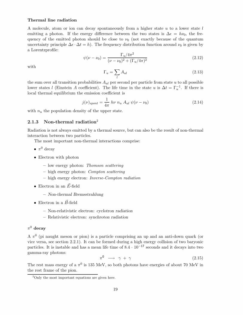
Thermal line radiation

A molecule, atom or ion can decay spontaneously from a higher state u to a lower state lemitting a photon. If the energy difference between the two states is Δε = hν0, the fre-quency of the emitted photon should be close to ν0 (not exactly because of the quantumuncertainty principle Δε ·Δt = h). The frequency distribution function around ν0 is given bya Lorentzprofile:

ψ(ν − ν0) =Γu/4π2

(ν − ν0)2 + (Γu/4π)2(2.12)

withΓu =

∑l

Aul (2.13)

the sum over all transition probabilities Aul per second per particle from state u to all possiblelower states l (Einstein A coefficient). The life time in the state u is Δt = Γ−1

u . If there islocal thermal equilibrium the emission coefficient is

j(ν)spont =14π

hν nu Aul ψ(ν − ν0) (2.14)

with nu the population density of the upper state.

2.1.3 Non-thermal radiation2

Radiation is not always emitted by a thermal source, but can also be the result of non-thermalinteraction between two particles.

The most important non-thermal interactions comprise:

• π0 decay

• Electron with photon

– low energy photon: Thomson scattering– high energy photon: Compton scattering– high energy electron: Inverse-Compton radiation

• Electron in an �E-field

– Non-thermal Bremsstrahlung

• Electron in a �B-field

– Non-relativistic electron: cyclotron radiation

– Relativistic electron: synchroton radiation

π0 decay

A π0 (pi naught meson or pion) is a particle comprising an up and an anti-down quark (orvice versa, see section 2.2.1). It can be formed during a high energy collision of two baryonicparticles. It is instable and has a mean life time of 8.4 · 10−17 seconds and it decays into twogamma-ray photons:

π0 −→ γ + γ (2.15)

The rest mass energy of a π0 is 135 MeV, so both photons have energies of about 70 MeV inthe rest frame of the pion.

2Only the most important equations are given here.

19

Figure 2.3: Radiation geometry (dotted line) of Thomson scattering for an unpolarised photonbeam.

Figure 2.4: Compton scattering event.

Thomson scattering

Photons can be scattered on free electrons. If the photon energy hν is much less than the restmass energy of the electrons mec

2, the frequency of the incoming photon is not changed, onlyits direction: elastic scattering. Consequently, thermal radiation will remain thermal afterscattering.

The probability of scattering is given by the electron density and the Thomson cross-section for electrons

σT ≡ 8π3r2e = 6.65 · 10−29 m2 (2.16)

with re the classical electron radius e2/mec2. The scattering is not equally strong in all

directions, the radiation geometry for unpolarised radiation has a typical dipole structure.The derivative of the Thomson cross-section to the solid angle Ω is[

dσT

dΩ

]unpol

=r2e2

(1 + cos2 θ) (2.17)

with θ the angle between the incoming and scattered radiation (see figure 2.3).

Compton scattering

If the photon energy is of the order of the rest mass energy of the electrons, the scatteringbecomes inelastic and energy and impulse is transferred from the photon to the electron. The

20

wavelength change is given byλ2 − λ1 = λc(1 − cos θ) (2.18)

with λc the Compton wavelength:

λc ≡ h

mec= 2.4 · 10−3 nm (2.19)

This energy loss is only important if λ1 ≈ λc, so for gamma-ray photons. In other cases thephoton is Thomson scattered.

The cross-section for this process is given by the Klein-Nishina equation:

σc(ε1, ε2) =r2e2

∫Ω

(ε2ε1

)2 (ε1ε2

+ε2ε1

− sin2 θ

)dΩ (2.20)

Question 2: Show that this equation is equal to the Thomson cross-section σT if ε2 = ε1.

Inverse-Compton radiation

The process described above can also be reversed: very energetic electrons transfer energyand momentum to (low energy) photons. This process can occur if the Lorentz factor γ ofthe electrons is (much) larger than 1, γ � 1. If the frequency of the incoming photon is ν1,with its direction of propagation making an angle θ with the velocity vector of the electron,the electron ’sees’ a frequency ν ′1 in its inertial system:

ν ′1 = γ(1 − v

ccos θ)ν1 (2.21)

If the photons are not too energetic (i.e. γhν1 � mec2) normal Thomson scattering will take

place in the rest frame of the electrons: ν ′2 = ν ′1. After transforming back to the observer’ssystem, the frequency of the scattered photon becomes:

νic = ν2 = ν1γ2(1 +

v

ccos θ′)(1 − v

ccos θ)

≈ 43γ2ν1 averaged over an isotropic radiation field (2.22)

≈ 4γ2ν1 head − on collision (2.23)

Consequently the electrons will slow down and the photons will gain energy rapidly. Theaverage power radiated by the electron in an isotropic photon field equals:

P =43σT γ2 Uph

v2

c(2.24)

with Uph the energy density of the photon field.In the observer’s inertial system the emitted radiation will be strongly beamed in the

forward direction, see figure 2.5. The beam width of the scattered photons is approximatelyproportional to γ−1. This effect is called relativistic beaming.

For a blackbody photon field

Uph =∫εnBB(ε) dε = nphε (2.25)

with nph the number density of the photon field and ε = hν = 2.7kT (see equation 2.7). Theaverage power P of equation 2.24 for relativisistic electrons (v ≈ c) can be rewritten as

P = cσTnphεic (2.26)

21

Figure 2.5: Radiation geometry of inverse-Compton radiation. The upper plots show theradiation geometry in the rest frame of the electron, the arrows indicate the direction of ac-celeration. The lower plots show the radiation geometry in the rest frame of the observer, theelectron velocity is along the horizontal axis.

which is self-explanatory if the cross-section for this process equals σT in the electron restframe.

Suppose that the energy distribution of the electrons is a power law in total energy3:

n(εtot)dεtot ∼ ε−αtot dεtot ⇔ n(γ)dγ ∼ γ−αdγ (2.27)

since ε = γmec2. The shape of the associated number spectrum of inverse-Compton scattered

photons can be easily derived from the relation

n(εic) = nphKe

∫σ(εic, ε, γ) γ−α dγ (2.28)

with Ke the normalisation constant for the electron energy distribution and σ(εic, ε, γ) thecross-section for producing a photon with energy εic from the scattering of an electron withLorentz factor γ on a blackbody photon with average energy ε. In this case we have

σ(εic, ε, γ) = σT δ

(εic − 4

3εγ2)

(2.29)

Question 3: Show that substitution of this cross-section yields:

n(εic) ∼ ε(α−1)/2 ε−(α+1)/2ic (2.30)

or n(νic) ∼ ν(α−1)/2 ν−(α+1)/2ic (2.31)

�Multiplication with hνic yields the shape of the energy density of the scattered photons:

ρ(νic) ∼ ν(α−1)/2 ν−(α−1)/2ic (2.32)

Non-thermal Bremsstrahlung

When a non-thermal electron is accelerated in an electric field, it will always emit Bremsstrahlung.If the electron distribution is non-Maxwellian (out of thermal equilibrium), equation 2.11 isnot valid. The emission coefficient will not depend on the temperature Te, but will depend onthe energy distribution of the electron beam. If the kinetic energy distribution of the electronsis a power law in electron kinetic energy:

N(εkin)dεkin ∼ ε−αkindεkin (2.33)

3Note that ε is used for a photon energy and ε is used for an electron energy

22

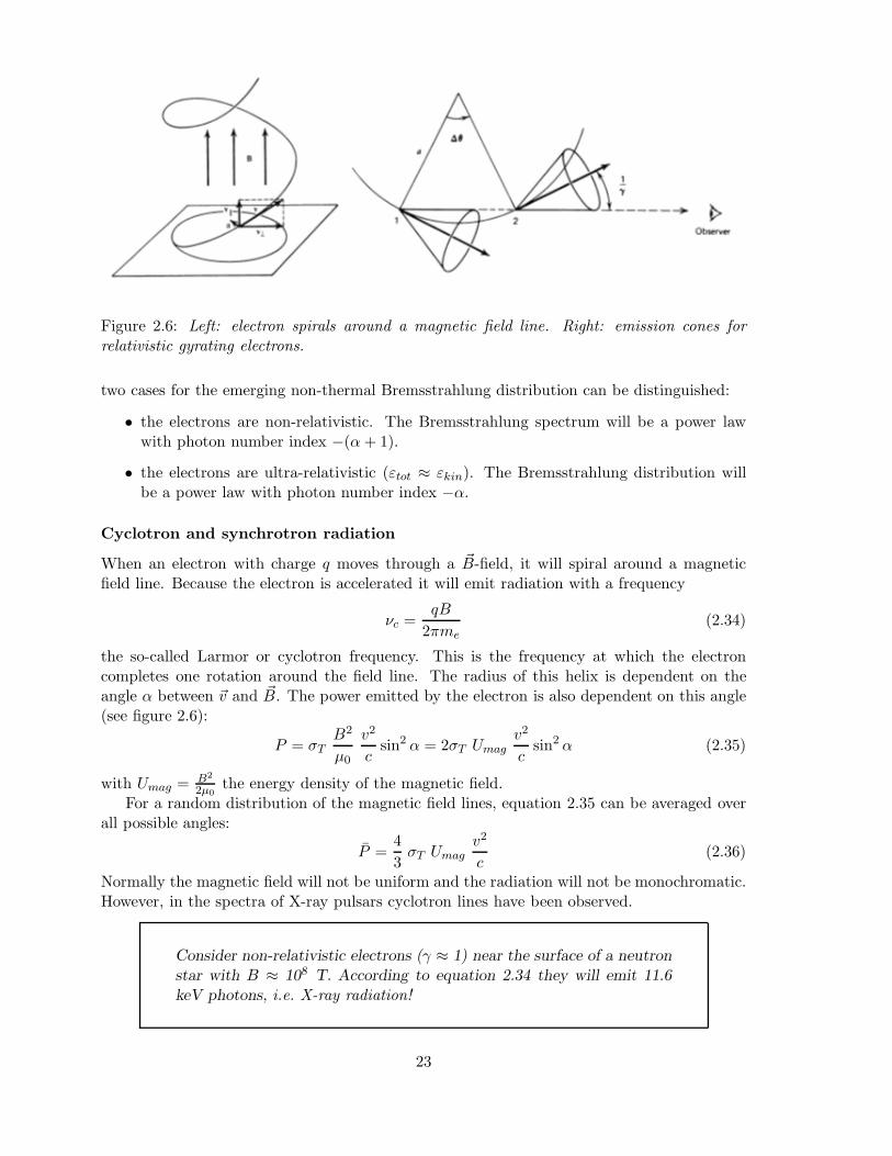
Figure 2.6: Left: electron spirals around a magnetic field line. Right: emission cones forrelativistic gyrating electrons.

two cases for the emerging non-thermal Bremsstrahlung distribution can be distinguished:

• the electrons are non-relativistic. The Bremsstrahlung spectrum will be a power lawwith photon number index −(α+ 1).

• the electrons are ultra-relativistic (εtot ≈ εkin). The Bremsstrahlung distribution willbe a power law with photon number index −α.

Cyclotron and synchrotron radiation

When an electron with charge q moves through a �B-field, it will spiral around a magneticfield line. Because the electron is accelerated it will emit radiation with a frequency

νc =qB

2πme(2.34)

the so-called Larmor or cyclotron frequency. This is the frequency at which the electroncompletes one rotation around the field line. The radius of this helix is dependent on theangle α between �v and �B. The power emitted by the electron is also dependent on this angle(see figure 2.6):

P = σTB2

μ0

v2

csin2 α = 2σT Umag

v2

csin2 α (2.35)

with Umag = B2

2μ0the energy density of the magnetic field.

For a random distribution of the magnetic field lines, equation 2.35 can be averaged overall possible angles:

P =43σT Umag

v2

c(2.36)

Normally the magnetic field will not be uniform and the radiation will not be monochromatic.However, in the spectra of X-ray pulsars cyclotron lines have been observed.

Consider non-relativistic electrons (γ ≈ 1) near the surface of a neutronstar with B ≈ 108 T. According to equation 2.34 they will emit 11.6keV photons, i.e. X-ray radiation!

23

The frequency of the radiation emitted by fast electrons in a magnetic field is lower thanthat of slow electrons due their relativistic mass increase. The rotation frequency (or gyro-frequency) is given by:

νg =νc

γ=

qB

2πγme(2.37)

and the averaged power has increased with a factor γ2:

P =43σT γ2 Umag

v2

c(2.38)

As in the inverse-Compton process, this radiation power is again strongly beamed. Theobserver will not see the radiation continously, but he will only see a short pulse wheneverthe electron is moving in his direction. The principal frequency of these pulses is called thesynchrotron frequency νs:

νs =32γ3νg sinα (2.39)

and is (much) larger than the gyro-frequency if γ � 1. These are very short pulses (γ−3 of arotation period). This pulse spectum will be broad and consists of many discrete components,i.e. the Fourier components of a sharp radiation pulse. This will blend into a real continuum,when the electrons have a velocity distribution, or when the magnetic field is not uniform,which is the practical case.

Since νs ∼ γ2, similar to the inverse-Compton process, the photon distribution functionis again a power law with spectral index (α + 1)/2 provided that the electrons have a powerlaw energy distribution with index α.

2.1.4 Astrophysical relevance

Radiation of black bodies is typically emitted in a broad band around the maximum wave-length

λmax =0.00290T

m (2.40)

For temperatures between 1 and 106 Kelvin, this radiation will thus fall between the near-radio (microwaves) and the extreme-ultraviolet (EUV). Cold objects (around 10 - 100 K),such as cool clouds of gas and dust, emit infrared waves. Normal stars are best observable inthe visible regime. Very hot objects (white dwarfs, neutron stars, supernova remnants) arepredominantly shining in the ultraviolet and soft X-ray regime. Large velocities are involvedfor the emission of harder X-rays.

Not only accreting neutron stars and black holes produce hard X-rays, also heavy starswith extended hot atmospheres, and hot diffuse gas in clusters of galaxies are good X-rayemitters.

Gamma-rays can not be formed in this way, much higher energy particles are needed, suchas cosmic-rays. When these particles interact with any atom, gamma-rays will be emitted.The main source of these photons are nebulae, dark molecular clouds and central parts ofgalaxies.

The inverse-Compton effect produces high energy photons. Their energy can be estimatedfrom equation 2.22 and 2.7 (

εic1 eV

)≈ 1200 Tz

(εe

1 GeV

)2

(2.41)

24

with εe = γmec2. If the cosmic background radiation (Tz = 2.7 K) is used as the incoming

radiation field, an electron of 550 MeV will boost the photon to 1 keV (X-rays). An electronof 550 GeV will produce a hard gamma-ray photon of 1 GeV.

Consider a proton (with mass mp) falling from infinity onto the surfaceof a compact star (massM∗, radius R∗). Its potential energy is convertedinto kinetic energy through:

12mpv

2 =GM∗R∗

mp =⇒ v =(

2GM∗R∗

)1/2

(2.42)

For a neutron star (M∗ = 1 M�, R∗ = 10 km), v ≈ 0.5c ! If all thiskinetic energy would be converted into thermal energy, an estimate ofthe maximum temperature Tmax follows from

kTmax =GM∗R∗

mp =⇒ Tmax ≈ 1012 K (2.43)

for a neutron star. For a white dwarf (M∗ = 1 M�, R∗ = 104 km) Tmax

amounts to ≈ 109 K.Consider next “bulk-mass” accretion flow onto the compact star witha rate M = dM

dt . The radiation luminosity arising from this bulk-massinfall into the gravitational potential well of the compact star is givenby

L =GM∗R∗

M (2.44)

An estimate of the effective temperature Te can now be obtained byemploying Stefan-Boltzmann’s law for a black body radiator with thetotal surface area of the compact star, i.e.

L =GM∗R∗

M = 4πR∗2σSBTe4 (2.45)

with σSB the Stefan-Boltzmann constant (= 5.67 · 10−8 W m−2 K−4).For an accretion rate M = 10−9 M� yr−1 this yields an effective temper-ature Te ≈ 107 K (L = 1030 W ) for a neutron star and Te ≈ 6 · 104 K(L = 1027 W ) for a white dwarf. Such temperatures make these ac-creting objects shine in the ultraviolet, extreme-ultraviolet (EUV) andX-ray wavelength regimes.

The energy range in which synchrotron photons are emitted, depends on the magneticfield strength and the typical electron energy εe = γmec

2. From equation 2.39 we find:(

εs1 eV

)≈ 0.07

(B⊥1G

)(εe

1 GeV

)2

(2.46)

So galaxies (B = 1 μG, εe = 1 GeV) are observable at radio frequencies.

25

A substantial part of the electromagnetic radiation of the Crab nebula is syn-chrotron emission. This radiation is observed over a very broad frequencyband,from radio- to gamma-waves. The typical magnetic field strength in this nebulais B ≈ 5 · 10−4 G, so the electrons which are involved should range from

Radio emission εs ≈ 10−7 eV (24 MHz) ⇒ εtot ≈ 50 MeV (γ ≈ 102)Gamma emission εs ≈ 1 GeV ⇒ εtot ≈ 5 PeV (γ ≈ 1010)

2.1.5 Multispectral correlations

To understand the source of radiation (the information source) better it is often enlighteningto look for multispectral correlations in the observed radiation fluxes. For instance: if anobserver wants to trace a dark (molecular) cloud, he can study the H, H2, CO or OH linesin the radio and infrared. But the cloud is potentially also visible in gamma-rays: primarycosmic-ray protons and heavy nuclei (see section 2.3.1) can interact with cloud gas, producingπ0-mesons which decay in γ-rays.

Synchrotron and inverse-Compton radiation are coupled through their generating electronbeams. This can already be seen from the similarities in the equations for the average power(2.24) and (2.38). When an electron beam travels through interstellar space, which has a verylow magnetic field (approximately 5 μG), both synchrotron radiation and inverse-Comptonradiation (from the cosmic background photons) are produced, but in a completely differentwavelength range: the synchrotron radiation will be emitted as radio waves and the inverse-Compton effect produces X-ray or gamma-ray photons. The energy ratio of the two waves is(using equations 2.41 and 2.46):

εicεs

= 2 · 104 Tz

(B⊥1 G

)−1

(2.47)

If a magnetic field B⊥ = 5 μG and Tz = 2.7 K are substituted, a ratio εic/εs = 1010 is obtained.

26

This equation can also be derived if the synchrotron process is described as a change of theelectron energy as a result of the magnetic field. This change is proportional to the magneticfield strength and the proportionality constant is the Bohr magneton:

μB =hq

2me(2.48)

The ratio (2.47) can then be calculated as

εicεs

=2.7kTz

μBB= 4 · 104 Tz

(B⊥1 G

)−1

(2.49)

The difference of about a factor of 2 in the numerical coefficient arises from the fact that theinverse-Compton and synchrotron spectra produced by a monochromatic electron beam arenot δ-functions but show a rather wide distribution. This has not been taken into account inthese ‘order of magnitude’ calculations.

2.1.6 Observing locations

There are two distinct ways of observation:

• In-situ, such as the

– geosphere, e.g. the magnetic field of the Earth

– sun, e.g. solar wind composition and velocity observations by a space probe (e.g.Ulysses, SOHO)

– planets, e.g. magnetic fields, atmosphere and rock composition (Viking, Pionier,Voyager, Mars Sojourner, Spirit, Opportunity)

• Remote sensing (or teledetection)

Remote sensing is the dominant technique for astronomical observations. During thepast several decades a very large number of observing facilities have been built which detectelectromagnetic waves from space.One major division between observing locations is ground-based and space-based. Both haveadvantages. Ground telescopes can in principle be

• larger (� 10 m diameter of the primary mirror)

• cheaper (80 – 100 M$, typically a factor 10 less than space telescopes)

• long lasting (≥ 50 year)

• easily accessible (changing instruments and refurbishment are ‘routine’)

• upgraded (install new, bigger and more complex detectors)

In contrast, space telescopes are more sensitive because they do not suffer from the atmosphereand the telescopes can more easily work at lower temperatures. Ground telescopes can onlyobserve in the radio and optical band. Only at some locations also observations in the infraredcan be done. Moreover, ground telescopes have only access to a limited part of the sky.

The main influence from the atmosphere is due to

27

• absorption

• emission

– black body radiation of atmosphere itself (infrared above 2 μm)

– variable OH emission lines (1 – 2 μm, 30 – 40 % variations within a few seconds)

This absorption and BB-emission is mainly caused by H2O in the atmo-sphere, but the H2O-content (and so the pressure P (z)) is a strong functionof altitude.

P (z) = P (z = 0) · e− zH (2.50)

with H the scaleheight, which is different for air and water:

Hair = 8000 mHwater = 3000 m

Observation at high altitudes (mountains, airplanes) gives large improve-ments in the thermal IR windows, but it does not reduce the OH emissionwhich is formed at about 90 km height.

• scattering due to dust

• scintillation and seeingWhen a plane coherent wave front travels through the Earth’s atmosphere, it encountersdensity variations due to turbulence and temperature differences. These inhomogeneitiesform cells with different indices of refraction, so that the wave front is distorted. These cellshave typical diameters of 10 cm and change with temporal frequencies between 1 and 1000Hz. So a 1 meter telescope sees about 100 of these cells changing potentially every 1 to 10milliseconds. Micro turbulence (even smaller scales) causes seeing. All this results in a highfrequency jitter of the image: a twinkling star!

Conditions for a good observing site are

• a stable atmosphere

• as high as possible

• on a island (water vapour is kept in a low inversion layer above the ocean)

• no pollution (dirt)

• no light pollution

Good sites are La Palma (Canary Islands, Spain), Hawaii (USA), La Silla and Paranal(Chili) and Kitt Peak (USA).

Space telescopes have two possible orbits, a high (or deep) and a low (near-earth) orbit.Low orbits are within the Van Allen radiation belts. It is relatively easy to put a high masstelescope in such an orbit which can be serviced by the Space Shuttle (e.g. the Hubble SpaceTelescope). But the orbit degrades and eventually the spacecraft will re-enter the atmosphere.

28

Moreover, it cannot observe a source for a long uninterupted time interval, because its loworbit around the earth gives rise to extended eclipses during each, typically 90 minute, orbitalperiod.

High orbit satelites suffer from extra noise due to solar flares and its detectors shouldbe radiation shielded. But it can observe a source for a long uninterupted period (24 – 100consecutive hours) and it has a real-time data link with a single ground station during almostits complete orbit (Example: ESA’s Infrared Space Observatory (ISO)).

2.2 Neutrinos


In particle physics all particles are divided in two groups: quarks and leptons. Moreover anti-particles of these types do also exist. All these particles have spin 1/2, they follow Fermi-Diracstatistics and are called fermions.

Single quarks have never been observed, but they constitute the building blocks of largerparticles, the hadrons. Several types of quarks are known and they are characterised by aflavour and a colour. Six flavours exist: up(u), down(d), strange(s), charm(c), bottom(b) andtop(t), and there are three colours, red(r), green(g) and blue(b).

d u s c b tMass (GeV) 0.004 - 0.008 0.002 - 0.004 0.08 - 0.12 1.15 - 1.35 4.1 - 4.4 170 - 190Charge (q) -1/3 +2/3 -1/3 +2/3 -1/3 +2/3Spin �J 1/2 1/2 1/2 1/2 1/2 1/2Baryon number 1/3 1/3 1/3 1/3 1/3 1/3

Table 2.1: Mass and quantum numbers of quarks.

Particles consisting of three quarks are called baryons, such as the proton (u-u-d, each adifferent color) and the neutron (u-d-d). Mesons are made up of two quarks, such as the pion(π meson) which consists of an up and an anti-down quark (or vice versa).

There are six types of leptons and anti-leptons. The lepton family consists of the electron(e−), muon (μ−), tau (τ−), electron-neutrino (νe), muon-neutrino (νμ) and the tau-neutrino(ντ ). The anti-lepton family consists of e+ (positron), μ+, τ+ and the anti-neutrinos νe, νμ

and ντ . Leptons do not have a color and they do not possess an electric or magnetic moment.They do not stick together to form other particles.

e νe μ νμ τ ντ

Mass (MeV) 0.511 ≤ 10 eV 105.66 ≤ 0.17 1784.1 ≤ 24Charge (q) -1 0 -1 0 -1 0Decay time (s) > 1029 2.2 · 10−6 3 · 10−13

Spin 1/2 1/2 1/2 1/2 1/2 1/2

Table 2.2: Mass, decay time and quantum numbers of leptons.

It is still not clear whether or not the neutrinos have a mass, although rather recently(1998) evidence was found that neutrinos should have at least some mass. Their existence

29

was derived because energy and impulse should be conserved in β-decay reactions, such as:

146C −→ 14

7N + e− + . . . (2.51)

If this were a two body process, conservation of energy and impulse would require that theelectron would always get a fixed velocity (two particles with two unknown velocities and twoconservation laws give a unique solution). But it was observed that there was a distribution ofelectron velocities. So a third particle needed to be invoked, the neutrino. Basically a neutronin the unstable core of the atom decays into a proton, an electron and an anti-neutrino:

n −→ p+ + e− + νe (2.52)

A muon-neutrino is formed during the decay of a muon or a pion:

μ± −→ e± + νe + νμ (2.53)π± −→ μ± + νμ (2.54)

Neutrino radiation is always characterised by its energy in electronVolts (eV).


Neutrinos from only two cosmic sources have been detected. Practically all detected neutrinosare produced in nuclear reactions in the core of the sun, such as:

p+ + p+ −→ 21H + e+ + νe (2.55)

137N −→ 13

6C + e+ + νe (2.56)

This last reaction is an example of β-decay which produces a positron.Another neutrino source was the supernova 1987A from which a pulse containing about

10 neutrinos was detected. These neutrinos are formed in the inverse β-decay process duringthe collapse of the core of the star:

p+ + e− −→ n + νe (2.57)


Neutrinos interact rarely with other particles and are consequently very difficult to detect.Large tanks of a suitable absorbing material are necessary. These should be located deeplyunderground (e.g. mines or mountains) to shield the neutrino telescope maximally againstnoise signals.

The first detector was built in 1968, comprising a large tank of tetracloroethene (C2Cl4), acheap cleaning agent. About 20 years later two watertanks, originally constructed to observepossible proton decay, turned out to be good neutrino detectors. These are the Kamiokandedetector in Japan and the Irvine-Michigan-Brookhaven (IMB) detector in the USA. A galliumbased detector was recently completed in the Gran Sasso tunnel (Appenine mountains) in Italy.

2.3 Cosmic-rays


Cosmic-rays (also energetic particles from the sun are sometimes included in cosmic radiation)consist mainly of atomic nuclei at very high velocities. Most particles are protons (84 %) and

30

helium nuclei (14 %), the rest are heavier nuclei, positrons and electrons. These have Lorentzfactors ranging from 2 to 1011. Cosmic-ray particles are always characterised by their energy(in electronVolts). For a particle which is more massive than a proton, its kinetic energy isusually given in energy per nucleon.

Electrons have a rest mass energy of 511 keV, protons have 938 MeV. The total energy oflarger particles with charge Z and mass M = Amp is

Ecr = γMc2 = Erestcr + Ekin

cr (2.58)

So the kinetic energy per nucleon of such a particle is given by

Ekincr

A= (γ − 1)mpc

2 (2.59)

A particle becomes relativistic when γ ≥ 2; an electron becomes relativistic, if its kineticenergy is above 0.5 MeV, a proton if its energy exceeds 1 GeV. Most cosmic-ray particlesincident on the Earth’s atmosphere have energies around 109 eV and a velocity of 0.9c. Theseso-called primary cosmic-rays have a flux of 104 particles per square meter per second. Theenergy spectra of cosmic-ray particles above 1 GeV show a typical power law dependence.This is shown in figure 2.7 for four species: H, He, C and Fe nuclei.


Cosmic-rays are presumably produced in supernovae and near the surface of pulsars. Theycan be accelerated in shocks (circumstellar and interstellar) and in pulsar magnetospheres.Their composition (including isotopic composition) near the Earth gives us important clues tocosmic acceleration and propagation phenomena and to the composition of interstellar clouds.


Primary particles cannot reach sea level and need to be observed from high-altitude-balloonsand space platforms. If such a primary cosmic-ray particle enters the earth’s atmosphere itwill collide with an air particle (predominantly N and O) at an average height of 30 to 60kilometer. This interaction produces a large number of different particles such as protons,neutrons, electrons, positrons, gamma photons, neutrinos, pions and muons. If the incomingparticle is sufficiently energtic (TeV (1012 ) to PeV (1015 ) energies), these secondary particleswill have sufficient energy to interact in turn with other particles, so a particle shower willreach the surface of the earth. These particles are called secondary cosmic-rays.

Also muons are detected as secondary particles which may seem puzzling, since their meantravel distance before they decay is about 660 meters according to Newtonian mechanics. Theyare formed at heights above 30 kilometer, but due to relativistic time dilatation it is possiblefor them to reach the ground before they decay.

The study of very-high-energy cosmic-rays by means of air shower production can thereforebe done from the ground with the aid of a so-called coincidence technique between severalradiation detector arrays.

2.4 Gravitational radiation


A mass m which is accelerated in a gravitational field due to a mass M emits gravitationalwaves. But since action = – reaction, both masses move in opposite directions, so the dipole

31

Figure 2.7: The differential energy spectra of cosmic-rays as measured from observations madefrom above the Earth’s atmosphere. The spectra for hydrogen, helium, carbon and iron areshown. The solid line shows the unmodulated spectrum for hydrogen, i.e. the effects of prop-agation through the interplanetary medium upon the energy spectra of the particles have beeneliminated using a model for the modulation process. The flux of the helium nuclei belowabout 60 MeV nucleon−1 is due to an additional flux of these particles which is known as theanomalous 4He component. This figure is taken from Longair (1992) and Simpson (1983).

part of the radiation cancels and the lowest order term becomes the quadrupole radiation.Except for the indirect measurement of gravitational waves from the binary pulsar PSR

B1913+16, for which Russell Hulse and Joseph Taylor shared the Nobel price in 1993, nodirect detection of gravitational radiation has yet been made. PSR B1913+16 comprises twoorbiting neutron stars with a period of 7.8 hours, one of the neutron stars is observable as aradio pulsar, with a period of 37.9 milliseconds. The shift in the times of periastron passagemeasured over 20 years with respect to a constant orbital period is shown in figure 2.8. Thegeneral theory of relativity predicts the curved solid line

32

Figure 2.8: Emission of gravitational radiation by PSR B1913+16 leads to an increasingdeviation in the time of the periastron passage compared with a hypothetical system whoseorbital period remains constant. Solid curve corresponds to the deviation predicted by thegeneral theory of relativity. Dots represent the measured deviation. The data provide thestrongest evidence now available for the existence of gravitational radiation.


According to the general theory of relativity, detectable gravitational waves should be emittedby a number of nearby, very close double star systems. Since the frequency of the signal isknown, detection of the periodic signal should be greatly facilitated, it is to be expected atrelatively low frequencies (10−4 – 1 Hz), corresponding to wavelengths in the range 3 · 108 –3 · 1012 m (the latter value being 20 times the distance from the Sun to the Earth!).


Ground-based detectors will search for signals from supernovae, compact binary coalescenceand pulsars at frequencies well above 1 Hz. The low-frequency range (below 1 Hz) willnever be accessible from the ground because it is masked by Earth-based gravitational noise.Moreover, there are several intrinsic uncertainties about the strength and distribution of allsources emitting higher frequencies.

Space-based observatories are required for frequencies below 1 Hz, moreover local closebinaries emitting at these low frequencies, are potentially assured sources. Supermassive blackholes, residing in the cores of active galaxies, do not radiate above 10−2 Hz and consequentlyalso require space-based detectors. Currently a space-based gravitational wave antenna (theLaser Interferometer Space Antenna LISA) is under development as a joint project betweenthe US(NASA) and Europe(ESA) for an anticipated launch in 2013.

33

Chapter 3

Stochastic Character of RadiationFields

3.1 Radiometric units

The spectral radiance or monochromatic intensity is the basic quantity to describe a radiationfield. It is defined as the amount of radiant energy per unit time, per unit area perpendicularto the beam, per unit solid angle, per unit wavelength (or frequency, energy). The relevantgeometry is displayed in figure 3.1, the spectral radiance is expressed as:

I(λ, �Ω, t) =dE

�n · �Ω dΩ dt dλ dA(3.1)

The monochromatic radiation flux density or spectral irradiance F (λ, t) is derived by integrat-ing I(λ, �Ω, t) over the solid angle:

Figure 3.1: geometry for defining intensity(radiance).

34

F (λ, t) =dE

dt dA dλ=∫Ω

I(λ, �Ω, t) �n · �Ω dΩ

=2π∫0

π∫0

I(λ, θ, φ, t) cos θ sin θ dθ dφ (3.2)

The total irradiance F (t) is subsequently obtained by integrating over all wavelengths.The spectral(monochromatic) radiant flux is the total amount of monochromatic radiant energythat is transported through a given area per unit time interval:

Φ(λ, t) =dE

dt dλ=∫Ω

∫A

I(λ, �Ω, t) �n · �Ω dΩ dA (3.3)

Finally, the radiant flux represents the total amount of radiant energy that is transportedthrough a given area, integrated over all wavelengths, per unit time:

Φ(t) =dE

dt=∫Ω

∫A

∫λ

Iλ(�Ω, t) �n · �Ω dΩ dA dλ (3.4)

For an isotropic radiation field from the upper hemisphere, e.g. an isotropically distributedsky background, the following relation holds:

F (λ, t) = πI(λ, �Ω, t) (3.5)

and for a point source at position �Ω0 with spectral radiance Sp(λ, t) the spectral irradianceis:

F (λ, t) =∫Ω

Sp(λ, t) δ(�Ω − �Ω0) �n · �Ω dΩ

= Sp(λ, t) �n · �Ω0 = Sp(λ, t) cos θ0 (3.6)= Sp(λ, t) for normal incidence (3.7)

The spectral radiance I, which characterizes the radiation beam, has intrinsic statistical fluc-tuations. As a consequence, an astronomical measurement has to be treated as a stochasticprocess.In the following paragraph, some basic statistical notions will first be reiterated, like thedefinition of random variables and the properties of frequently encountered probability dis-tributions. Next, the concept of a stochastic variable is introduced and some basic propertiesare discussed. These will be used later for describing the astronomical measuring process.

3.2 Random phenomena and variables

3.2.1 Parent population

A random phenomenon is characterized by the fact that the outcome, in terms of a numer-ical value, is not predictable in a deterministic sense, but exhibits a more or less smoothdistribution of outcomes if repeated many times. Associated with this notion is the random

35

variable (RV), which value constitutes a numerical outcome of a certain random phenomenon.The probability density distribution of a random variable gives the possible values and theprobabilities assigned to these values.Random variables can be subdivided in two categories:

• Discrete random variables, comprising a finite number of possible values.

• Continuous random variables, comprising all values in a certain number interval, i.e. aninfinite number of possible values.

If an infinite number of measurements could be taken, the result would give the way in whichthe observed data points are distributed, i.e. the true probability distribution. This distribu-tion is called the parent distribution, practical measurements can be hypothesized as samplesof an infinite number of possible measurements which are distributed according to the parentpopulation. In other words the parent population parameters can be perceived to becomeequal to the experimental parameters in the limit of an infinite number of measurements:

(Parent parameter) = limN→∞

(experimental parameter) (3.8)

If N measurements are made of a quantity x, labeled x1, x2, ..., xN , the mean μ of the parentpopulation can be defined as:

μ ≡ limN→∞

(1N

∑i

xi

)(3.9)

The mean is therefore equivalent to the centroid or average value of the quantity x.The median value μ1/2 of the parent distribution is that value at which there are equal

numbers of values higher and lower than μ1/2. Expressed differently, the probability thatan arbitrarily selected value is higher than the median is 50%, and the probability that anarbitrarily selected value is lower is 50% also:

P (xi > μ1/2) ≡ P (xi < μ1/2) ≡ 0.5 (3.10)

Finally, the most probable value μmax of the parent distribution is the value at which thedistribution peaks:

P (μmax) ≥ P (xi �= μmax) (3.11)

For symmetric distributions, like the Gauss function, the average, median and most prob-able value are all the same. The differences are only visible in asymmetric functions, as inFigure 3.2.

An appropriate measure of the dispersion of observations is the standard deviation σ. Thevariance σ2 is defined as the limit of the average of squares of the deviations from the meanμ:

σ2 ≡ limN→∞

[1N

∑i

(xi − μ)2]

= limN→∞

(1N

∑i

x2i

)− μ2 (3.12)

36

Figure 3.2: Illustration of the various definitions of ”average”, illustrated for the Maxwelliandistribution function f(x) = x2G(x, 0, 25) where G(x, μ, σ) is the Gauss-function of equation3.27.

3.2.2 Discrete and continuous distributions: expectation values

If there are n different observable values of a discrete random variable x, expression (3.9) canbe replaced by:

μ =n∑

j=1

xjP (xj) (3.13)

where P (xj) is the probability to obtain the discrete value xj and no two values of xj areequal. Similarly, the definition of the variance can be redefined in terms of the probabilityfunction P (xj):

σ2 =n∑

j=1

[(xj − μ)2P (xj)

]=

n∑j=1

[x2

jP (xj)]− μ2 (3.14)

The mean μ is the expectation value E{x} of x, and the variance σ2 is the expectation valueE{(x− μ)2} of the square of the deviations of x from μ.The expectation value of any function f(x) of x is given by

E{f(x)} =n∑

j=1

[f(xj)P (xj)] (3.15)

If the parent distribution is considered as a continuous, smoothly varying function p(x),the mean μ and the variance σ2 are given by the following integral expressions:

μ =+∞∫

−∞xP (x)dx and σ2 =

+∞∫−∞

x2P (x)dx− μ2 (3.16)

37

Figure 3.3: Illustration of the difference between the parent distribution and the distributionderived from a finite number of measurements, in this case 100 trials displayed with the his-togram. The solid curve is the actual parent distribution, a Gaussian distribution with averageμ = 3.000 and standard deviation σ = 1.000. The dashed curve is the estimated parent distri-bution derived from the histogram with parameters x = 3.045 and s = 1.078.

The expectation value of any function f(x) of x follows from:

E{f(x)} =+∞∫

−∞f(x)P (x)dx (3.17)

3.2.3 Sample parameters

In practical experiments, only a finite number of observations will be made. Consequently,the experimental data only allow an estimate of the parameters of the parent distribution.For a series of N observations, the most probable estimate of the mean μ is the average x ofthe observations (see a later paragraph on the method of maximum likelihood). Hence:

μ ≈ x ≡ 1N

∑i

xi =1N

n∑j=1

fjxj (3.18)

with fj the number of times each value of xj is observed, no two values of xj being alike. Thisaverage x is called the sample mean and is distinctly different from the parent mean μ.The best estimate of the parent variance σ2 is given by the experimental or sample variances2, according to:

σ2 ≈ s2 ≡ 1N − 1

∑i

(xi − x)2 =1

N − 1

n∑j=1

fj(xj − x)2 (3.19)

38

Figure 3.4: (Left) Binomial distribution function for flipping a coin (10x) PB(k, n, p): n = 10and p = 1/2; μ = 5 and σ = 1.6. (Right) Binomial distribution function for throwing 10 dicePB(k, n, p): n = 10 and p = 1/6; μ = 1.67 and σ = 1.2.

where the factor N − 1 in the denominator is the number of degrees of freedom left forassessing s2 after determining the value of x from N observations. Again, the value of thesample variance s2 is distinctly different from the parent variance σ2 unless N → ∞.

Figure 3.3 shows the deviations between parent mean and sample mean, parent standarddeviation and sample standard deviation respectivily, for a sample of 100 measurements. Themagnitude of the errors in sample mean and variance is obviously dependent on the size ofthe sample. A quantitative estimate of these errors will be discussed later in this chapter.

3.3 Probability density distributions

In this section the probability density distributions are reviewed that often occur, or arepostulated to occur, in measurement series.

3.3.1 The binomial and Poisson distributions

An observer tries to detect photons during a certain time interval. The expected numberof photons to arrive in this interval is μ. How many photons will the observer detect? Toaddress this question, the measurement interval is subdivided in n equal sub-intervals. In eachsub-interval the probability that a photon arrives is therefore p = μ/n (a correction to thisstatement follows below!), the probability that no photon arrives is 1 − p. The measurementof the observer can thus be considered as a series of n trials to find a photon, each trial havingprobability p of succeeding. The probability that k photons will be detected is then given bythe binomial function:

PB(k, n, p) =

(nk

)pk(1 − p)n−k (3.20)

The binomial function also describes processes like flipping a coin, or throwing dice. Forexample, when a coin is flipped the probability of getting head is p = 1/2, and the probability

39

of getting k times head when the coin is flipped 10 times is given by PB(k, 10, 0.5), thisillustrated at the left in figure 3.4. When we throw 10 dice, the probability of getting k timesa 1 is given by PB(k, 10, 1/6), illustrated at the right in figure 3.4.The mean μ of a binomial distribution can be evaluated by combining the definition of μ asthe first moment of the distribution function and expression (3.20):

μ =n∑

k=0

[k

n!k!(n− k)!

pk(1 − p)n−k]

= np (3.21)

Likewise, the variance σ2 of a binomial distribution is computed by considering the expectationvalue of (k − μ)2:

σ2 =n∑

k=0

[(k − n)2

n!k!(n − k)!

pk(1 − p)n−k]

= np(1 − p) (3.22)

Note: evaluate these sums yourself!The results for the mean μ and the variance σ are remarkably simple. If the probability for asingle success p is equal to the probability for failure p=1−p=1

2 , the distribution is symmetricabout the mean μ, and the median μ 1

2and the most probable value are both equal to the

mean. In this case the variance σ2 is equal to half the mean: σ2=μ/2. If p and q=1 − p arenot equal, the distribution is asymmetric with a smaller variance.Return now to the experimenter measuring the arrival of photons. If the sub-interval is large,there is a finite probability that more than 1 photon will arrive in this particular interval,which is not taken into account in the above argument. To suppress this probability, the limitis taken of letting the number of trials n go to infinity, keeping the product np ≡ μ constant.In this limit the binomial distribution changes into the Poisson distribution, in which theprobability of obtaining k photons is given by

PP (k, μ) =μk

k!e−μ (3.23)

The derivation of this expression follows from:

P (k) =

(nk

)pk(1 − p)n−k =

n!k!(n − k)!

(μ

n

)k (1 − μ

n

)n−k

(3.24)

=μk

k!n(n− 1)(n − 2)..(n − k + 1)

nk

(1 − μ/n)n

(1 − μ/n)k=μk

k!1e−μ

1=μk

k!e−μ

The exponent makes sure that the sum∑PP (k, μ) over all probabilities from k = 0 to k = ∞

is 1 (remember ex = 1 + x+ x2/2! + x3/3! . . . .).Suppose the observer carries out an infinite number of observations (this is obviously a

thought experiment), and should then on average detect μ photons: k = μ. The varianceσ2 ≡ (k − μ)2 also equals μ.The derivations of these results follow from:

k =∞∑

k=0

kμk

k!e−μ = e−μ(0 + μ+ 2

μ2

2!+ . . .) = e−μ(μ+

μ2

1!+μ3

2!. . .) (3.25)

= e−μμ(1 +μ

1!+μ2

2!+ . . .) = e−μμeμ = μ

40

Figure 3.5: (Left) Poisson distribution function PP (k, μ) for μ = 5. (Right) Poisson distribu-tion function PP (k, μ) for μ = 1.67. The dotted lines show Gaussian approximations to thePoisson function.

∞∑k=0

k2μk

k!= 0 + μ+ 2μ2 + 3

μ3

2!.. = μ(1 +

μ

1!+ 3

μ2

2!..) = μ(1 +

μ

1!+μ2

2!+ ..

μ

1!+ 2

μ2

2!+ ..)

= μ(eμ + μ[1 +μ

1!+μ2

2!+ ..]) = μeμ + μ2eμ (3.26)

hence

σ2 ≡ (k − μ)2 =∞∑

k=0

k2P (k) − μ2 = e−μ∞∑

k=0

k2μk

k!− μ2 = μ+ μ2 − μ2 = μ

Two examples of the Poisson distribution are given in figure 3.5. The dotted lines in-dicate Gaussian approximations to the Poisson function. It is clear from these examplesthat especially for low values of the mean μ, the Gaussian approximations underestimate theprobability of large deviations!

3.3.2 The Normal or Gaussian distribution

If μ is large, the Poisson distribution is well approximated by the normal distribution, alsocalled the Gaussian distribution:

PG(x, μ, σ) =1

σ√

2πexp

[−1

2

(x− μ

σ

)2]

(3.27)

for the special case where σ =√μ. The Gauss function has the computational advantage over

both the binomial and the Poission distribution that it is easy to compute; it does not containsuch expensive calculations as the factorials. It also describes (or is assumed to describe) thedistribution of measurements in many physical experiments.The shape of the distribution is illustrated in figure 3.6. It is a bell-shaped curve symmetricabout the mean μ. The width of the distribution is characterized by the full-width at half-maximum, which is generally called the half-width Γ. This is defined as the range of x between

41

Figure 3.6: Gaussian probability distribution PG(x, μ, σ) versus x−μ; Γ = 2.354σ and P.E. =0.6745σ.

the values at which the probability PG(x, μ, σ) is half its maximum value:

PG(x± 12Γ, μ, σ) =

12PG(μ, μ, σ) Γ = 2.354σ (3.28)

A tangent drawn along the portion of steepest descent of the curve intersects the curve at thee−

12 points x=μ± σ and intersects the x-axis at the points x=μ± 2σ:

PG(μ± σ, μ, σ) = e−12PG(μ, μ, σ) (3.29)

The mean and standard deviation of the Gaussian distribution are equal to the parametersμ and σ given explicitly in the probability density equation (3.27). This equivalence can beverified by using the definitions of μ and σ as the expectation values of x and (x − μ)2 forcontinuous distributions, as discussed in the previous paragraph.The probable error P.E. is defined to be the absolute value of the deviation |x− μ| such thatthe probability for the deviation of any random observation |xi−μ| to be less is equal to 1

2 . Inother words, half the observations of an experiment are expected to fall within the boundariesdenoted by μ±P.E.. The relation between the P.E. and the standard deviation σ is found byevaluating the point at which the integral probability curve yields a probability of 1

2 of beingexceeded.

3.3.3 The Lorentzian distribution

The Lorentzian distribution is frequently encountered in spectroscopic data reduction, sinceit describes the resonance behaviour associated with atomic and nuclear transitions. Theprobability density function is displayed in figure 3.7 and defined as:

PL(x, μ,Γ) =1π

Γ/2(x− μ)2 + (Γ/2)2

(3.30)

42

Figure 3.7: The Lorentzian probability distribution for μ = 25 and Γ = 5.

The distribution is symmetric about its mean μ, with a half-width Γ. The most noticabledifference with the Gaussian distribution is the fact that it does not diminish to zero so rapidly,for large deviations it only decreases proportional to the square of the deviation.The mean μ is one of the free parameters, it is also equal to the median and the mostprobable value, like in the case of the Gaussian distribution. However, the standard deviationis not defined for a Lorentzian distribution as a consequence of its slowly decreasing behaviourfor large deviations, i.e. the integral defining the expectation value for the square of thedeviations is unbounded. The width of a Lorentzian distribution is characterized by the half-width parameter Γ, defined such that when the deviation from the mean x − μ = Γ/2, theprobability density PL(x, μ,Γ) is half its value at the maximum. Note: verify this yourself!

Figure 3.8 shows a comparison of the Gaussian and Lorentzian distributions with equalvalues for their means μ and half-widths Γ.

3.4 Method of maximum likelihood

3.4.1 Calculation of the mean

Consider an observation that comprises a set of N data points, and is presumed to be a ran-dom selection from a Gaussian parent distribution PG(xi, μ, σ). How does one arrive at anestimate μ′ from the data, giving the maximum likelihood that the parent distribution had amean equal to μ, and what is the error in the estimate μ′?If we hypothesize a trial parent distribution PG(xi, μ

′, σ), the probability of observing a par-

43

Figure 3.8: Lorentzian probability distribution PL(x, μ,Γ) versus x−μ, compared to a Gaussiandistribution with the same mean and half-width.

ticular value xi for one of the data points is given by

PG(xi, μ′, σ) =

1σ√

2πexp

[−1

2

(xi − μ′

σ

)2]

(3.31)

Considering now the entire set of N observational values, the probability for observing thatparticular set is given by

P (μ′, σ) =N∏

i=1

PG(xi, μ′, σ) =

(1

σ√

2π

)N

exp

[−1

2

∑i

(xi − μ′

σ

)2]

(3.32)

According to the method of maximum likelihood, when comparing P (μ′, σ) for several valuesof μ′, the most likely parent population from which such a set of data might have come, i.e.when P (μ′, σ) is at the maximum value, is assumed to be the correct one.The value P (μ′, σ) in equation (3.32) is maximum if the exponential term is minimized, hence:

−12d

dμ′∑

i

(xi − μ′

σ

)2

= 0 =⇒ μ′ = x ≡ 1N

∑i

xi (3.33)

In practise, some data points might be measured with better or worse precision than others,this can be accomodated by assigning to each data point xi its own standard deviation σi,representing the precision with which that particular data point was measured, hence:

−12d

dμ′∑

i

(xi − μ′

σi

)2

= 0 =⇒ μ′ =∑

i(xi/σ2i )∑

i(1/σ2i )

(3.34)

The most probable value for the mean is therfore the weighted average of the data points,each data point being weighted inversely by its own variance.

44

3.4.2 Estimated error of the mean

What uncertainty σμ is associated with the estimate of the mean μ′ in equation 3.34?Each individual variance σ2

i contributes some uncertainty; assuming uncorrelated measure-ment points xi the accumulated variance σ2

μ of the estimated mean μ′ follows from:

σ2μ =

∑i

[σ2

i

(∂μ′

∂xi

)2]

(3.35)

if higher-order terms in the expansion of σ2μ are neglected. The values of the partial differential

quotients ∂μ′/∂xi can be derived from expression 3.34:

∂μ′

∂xi=

1/σ2i∑

i

(1/σ2

i

) =⇒ σ2μ =

1∑i

(1/σ2

i

) (3.36)

If the uncertainties in the data points are all equal, i.e. if σi = σ, the error of the meanreduces to the simple expression:

σ2μ =

σ2

N(3.37)

Example: Consider the sample displayed in figure 3.3 of a previous paragraph, that comprises100 measurements. The mean was estimated to be μ ≈ μ′ = x=3.045, the standard deviationwas estimated to be σ ≈ s=1.078. Since all the uncertainties σ in the individual data pointsare equal, the uncertainty in the determination of the mean equals σμ ≈ s/

√N=0.108. This

is already substantially larger than the actual error of 0.045.Important notion: If the discrete values of x in figure 3.3, i.e. the centres of the verticalbins at 0.25, 0.75, 1.25,....., 5.75, are not the exact trial values but merely reflect the lumpingof trial values in bin widths of 0.5 straddling these centre values, the exact numerical resultson the sample mean x and the sample standard deviation s will depend on the selected binwidths (0.5 in this case)and the bin grid (centre values of x). The choice of the appropriatebin widths in data acquisition and handling is the subject of optimal sampling, which will bediscussed in Chapter 5.

3.5 Stochastic processes

3.5.1 Distribution functions

A stochastic process is defined as an infinite series of stochastic variables, one for each value ofthe time t. For a specific value of t, the stochastic variable X(t) possesses a certain probabilitydensity distribution. The numerical value of the stochastic variable X(t) at time t correspondsto a particular draw (outcome) from this probability distribution at time t. The time seriesof draws represents a single time function and is commonly referred to as a realisation of thestochastic process. The full set of all realisations is called the ensemble of time functions (seeFig. 3.9).At each time t, the stochastic variable X(t) describing the stochastic process, is distributedby a momentary cumulative distribution, called the first-order distribution:

F (x; t) = P{X(t) ≤ x}, (3.38)

which gives the probability that the outcome at time t will not exceed the numerical value x.The probability density function, or first-order density, of X(t) follows from the derivative of

45

Figure 3.9: The ensemble of time functions of a stochastic process.

F (x; t),

f(x; t) ≡ ∂F (x; t)∂x

. (3.39)

This probability function may be a binomial, Poisson or normal (Gaussian) distribution.

3.5.2 Mean and variance

For the determination of the statistical properties of a stochastic process it suffices in manyapplications to consider only certain averages, in particular the expected values of X(t) andof X2(t).

The mean or average μ(t) of X(t) is the expected value of X(t) and is defined as

μ(t) = E{X(t)} =+∞∫

−∞x f(x; t) dx. (3.40)

The variance of X(t) is the expected value of the square of the difference of X(t) and μ(t)and is, by definition, equal to the square of the standard deviation:

σ2(t) = E{(X(t) − μ(t))2} = E{X2(t)} − μ2(t) (3.41)

(in case of real functions X(t) and μ(t)).

3.6 Intrinsic stochastic nature of a radiation beam

3.6.1 Bose-Einstein statistics

Irrespective of the type of information carrier, e.g. electromagnetic or particle radiation, theincoming radiation beam in astronomical measurements is subject to fluctuations which derivefrom the incoherent nature of the emission process in the information (=radiation) source. For

46

a particle beam this is immediately obvious from the corpuscular character of the radiation,however for electromagnetic radiation the magnitude of the fluctuations depends on whetherthe wave character or the quantum character (i.e. photons) dominates. By employing Bose-Einstein statistics, the magnitude of these intrinsic fluctuations can be computed for thespecific case of a blackbody radiation source, which is incoherent or “chaotic” with respect totime.In this course we shall not embark on a detailed treatment of these fluctuations, this is a subjectthat will be elaborated in the more advanced course Observational Astrophysics 2 (OAF2). Itsuffices here to give the outcome of applying Bose-Einstein statistics to a blackbody radiationfield:

• For a photon energy hν � kT , the statistical fluctuations in the radiation beam aredominated by the wave character of the radiation. If the average radiation power perunit frequency interval is given by P (ν) (e.g. in Watt Hz−1), the variance in this poweris given by:

ΔP 2(ν) = P2(ν) (3.42)

and P (ν) = kT (3.43)

The value of P (ν) applies to one degree of polarisation!This case is called the thermal limit for an electromagnetic radiation beam.

• In the other extreme case that hν � kT , photon statistics prevails and the statisticalfluctuations in the signal can be expressed as Poissonian noise:

Δn2(ν) = n(ν) (3.44)

in which n(ν) represents the number of photons in the observation sample. This con-dition is called the quantum limit of the fluctuations and it represents the minimumvalue of intrinsic noise present in any radiation beam. Obviously, this always holds forcorpuscular radiation (cosmic-rays) and neutrinos, since the wave character is not anissue.

Figure 3.10 shows the subdivision between thermal and quantum noise as a function of tem-perature. The transition between noise in the quantum limit to the thermal limit occurs athν ≈ kT . At room temperature, T ≈ 300 K, this corresponds to a frequency ν ≈ 6 THz, ora wavelength λ ≈ 50 μm. The relation ν = kT/h as a function of temperature T is displayedin figure 3.10. It is clear from this diagram that radio observations are always dominated bythe wave character of the incoming beam and are therefore performed in the thermal limit.As a result, the treatment of noise in radio observations differs drastically from that of mea-surements at shorter wavelengths. Specifically at submillimetric and infrared wavelengthsquantum limited observation is vigorously pursued but this remains still difficult.

The fluctuations in average power P (ν), given in equation 3.42 for the thermal limit canbe interpreted in such a way that whenever wave packet interference becomes important, theinterference will cause the fluctuations to become of the same magnitude as the signal. Thelow frequency fluctuations can be thought of as caused by the random phase differences andbeats of the wavefields, as described in the following paragraph.Note:The above expression for the fluctuations in a blackbody photon gas applies only to theinterior of a blackbody in which the receiving element is submerged, i.e. a blackbody cavity

47

Figure 3.10: Frequency as a function of temperature: division between thermal and quantumnoise. Figure taken from Lena (1988).

or a thermal bath. This requires that the condition λ2 = c2/ν2 = AeΩ is satisfied, in whichAe represents the effective collecting area of the telescope and Ω the solid angle subtented bythe radiation source. The expression AeΩ is called the throughput or ”etendue” of coherence.(The derivation of this relation and the subject of coherent detection will be treated in detaillater in OAF2). If this condition is not fulfilled, then even in the limit hν � kT quantum noisemay dominate. For example, if a star, whose spectrum resembles a blackbody at temperatureT , is observed at frequency ν, such that hν � kT , thermal noise ought to dominate. Thestar may however be so distant that the radiation is effectively unidirectional and hence,AeΩ � λ2. The photons will consequently arrive well separated in time and quantum noiseevidently dominates.

3.6.2 Electromagnetic radiation in the thermal limit

In astrophysics, many sources of electromagnetic (EM) radiation have a thermal origin. Thisimplies that the incoming wave-signal has been built up by the superposition of many indi-vidual wavepackets, which were all generated by a myriad of independent radiative atomictransitions at the radiation source. Each wavepacket has a limited duration that dependson the characteristic time scale of the particular atomic transition. The intrinsic spread inthe frequency of the emitted wavepacket derives from the uncertainty relation of HeisenbergΔεΔt = h with spread in frequency Δν = 1/Δt. The characteristic time length of such awavepacket Δt ≡ τc = 1/Δν is called the coherence time, it represents the typical time scaleover which the phase of the EM-wave can be predicted with reasonable accuracy at a givenlocation in space. Figure 3.11 shows the stochastic signal comprising a random superpositionof individual wavepackets. This wave signal fluctuates both in amplitude and in frequency,

48

Figure 3.11: A quasi-monochromatic wave.

the latter characterised by a typical bandwidth Δν around an average frequency ν. Such asignal represents a quasi-monochromatic wave with a frequency stability ν/Δν.

The frequency bandwidth Δν can be accommodated by introducing a complex waveamplitude1 E0(t) =| E0(t) | ·eiφ(t), which involves a time dependent phase angle φ(t). Theelectromagnetic wave can then generally be expressed as follows:

E(t) = E0(t) · ei2πνt =|E0(t) | · ei(2πνt+φ(t)) (3.45)

Taking the real part for one direction of polarisation, this equation becomes

E(t) = E0(t) cos(2πνt+ φ(t)) (3.46)

The stochastic variable describing the radiation field in the thermal limit is thus representedby the time variable electric field vector E(t), i.e. X(t) = E(t). A full treatment of thestochastic properties of a thermal radiation field is given in OAF2.The time dependent behaviour of E(t) is depicted in figure 3.11 representing one polarisationcomponent of a quasi-monochromatic wave. Points on the EM-wave shown in this figureseparated by more than τc in time are related to different wavepackets and show therefore nocorrelation in phase.

At optical wavelengths, a typical atomic transition takes τc ≈ 10−9 s, this comprises aboutone million oscillations at a typical carrier frequency of 1015 Hz, i.e. the fluctuation frequenciesof |E0(t) | and φ(t) for quasi-monochromatic radiation are much slower than ν.

1A tilde is put over quantities that are explicitly used as complex variables to avoid confusion

49

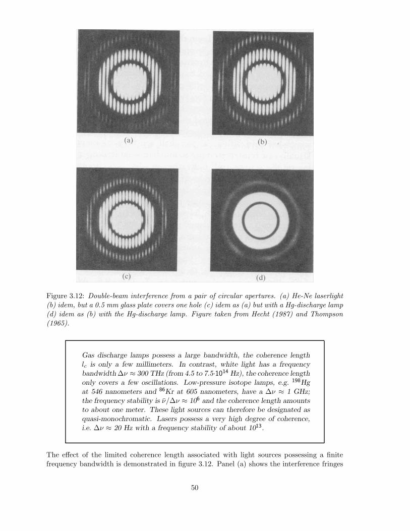
Figure 3.12: Double-beam interference from a pair of circular apertures. (a) He-Ne laserlight(b) idem, but a 0.5 mm glass plate covers one hole (c) idem as (a) but with a Hg-discharge lamp(d) idem as (b) with the Hg-discharge lamp. Figure taken from Hecht (1987) and Thompson(1965).

Gas discharge lamps possess a large bandwidth, the coherence lengthlc is only a few millimeters. In contrast, white light has a frequencybandwidth Δν ≈ 300 THz (from 4.5 to 7.5·1014 Hz), the coherence lengthonly covers a few oscillations. Low-pressure isotope lamps, e.g. 198Hgat 546 nanometers and 86Kr at 605 nanometers, have a Δν ≈ 1 GHz;the frequency stability is ν/Δν ≈ 106 and the coherence length amountsto about one meter. These light sources can therefore be designated asquasi-monochromatic. Lasers possess a very high degree of coherence,i.e. Δν ≈ 20 Hz with a frequency stability of about 1013.

The effect of the limited coherence length associated with light sources possessing a finitefrequency bandwidth is demonstrated in figure 3.12. Panel (a) shows the interference fringes

50

Figure 3.13: Staircase function.

when two small circular apertures are illuminated by a He-Ne laser source. Panel (b) showsthe fringe patters when one of the apertures is covered with an optically flat piece of glas witha thickness of 0.5 mm. No change in the form of the pattern, other than a shift in its location,is evident because the coherence length of the laser light far exceeds the optical path-lengthdifference introduced by the glass plate. On the other hand, when the same experiment isrepeated using the light of a collimated Hg-discharge lamp, the fringes disappear (comparepanel (c) and (d)). In this case the coherence length of the beam is appreciably shorter thanthe optical path difference introduced by the glass plate. Hence, the wavepackets emanatingfrom the two apertures are uncorrelated and no fringe pattern is formed.

3.6.3 Electromagnetic radiation in the quantum limit

In the quantum limit no coherence effects occur and the radiation field fluctuations can bedescribed by photon statistics only. Consider an incident radiation beam with an average fluxof nb photons (or particles or neutrinos) per second. The generation of photons at randomtimes ti can be described by a stochastic variable X(t), which consists of a family of increasingstaircase functions, with discontinuities at the the points ti, see figure 3.13:

X(t) =∑

i

U(t− ti) (3.47)

with U(t) the unit-step function

U(t) =

{1 for t ≥ 00 for t < 0.

(3.48)

The derivative of the stochastic variable X(t):

Y (t) =dX(t)dt

=∑

i

δ(t− ti) (3.49)

represents a train of Dirac impulses at random time positions ti. The number of photons XΔT

registered during a measurement period ΔT (which is a (small) part of the total measurementtime T ), follows from

XΔT =t+ΔT∫

t

∑i

δ(t − ti) dt = k (3.50)

51

The random variable XΔT is distributed according to a Poisson distribution. The probabilityto detect k photons, if the mean value is μ, is:

pP (k, μ) =μk

k!e−μ (3.51)

with k an integer value. The (continuous) probability density function for Poissonian statisticscan now be expressed as:

p(x, μ) =∞∑

k=0

pP (k, μ) δ(x − k) (3.52)

So, the average value of XΔT is:

E{XΔT } =+∞∫

−∞x p(x, μ) dx = μ = nb ΔT (3.53)

The variance σ2 of a Poisson distribution equals the average μ, i.e. nb ΔT , the standarddeviation σ is

√nb ΔT . The signal to noise ratio (S/N) can be defined as μ/σ =

√nb ΔT .

Given an average flux of nb, the value of S/N thus improves with the measurement periodΔT proportional to (ΔT )

12 . In an analogous fashion the S/N of the stochastic variable Y (t)

improves with n12b .

52

Chapter 4

Physical principles of radiationdetction

4.1 Types of detection

Detection of a radiation field can generally be subdivided in two categories: amplitude detec-tion and power detection.

4.1.1 Amplitude detection

This type of detection involves the measurement of the instantaneous amplitude of an elec-tromagnetic wave with average frequency ν and varying amplitude and phase. Consideringone component of polarisation, the signal S(t) varies as

S(t) = E0(t) cos(2πνt+ φ(t)) (4.1)

and is obtained by conversion of the electromagnetic field into a current by a receiving antenna.The relation between the signal and the amplitude of the wave can be regarded as linear,moreover the phase information φ(t) remains available. This detection process is thereforereferred to as coherent detection.

4.1.2 Power (or intensity) detection

In this case the detection process involves the measurement of the average power of an elec-tromagnetic wave, a particle or a neutrino beam, in which the averaging takes place over acertain time interval ΔT , i.e. the detection yields a running average over ΔT . For electro-magnetic waves this integration interval ΔT is large compared to the period of the wave c/ν,the signal S(t) follows from:

S(t) =1

ΔT

t+ΔT∫t

E(t′) · E∗(t′) dt′ =1

ΔTΠ(

t

ΔT

)∗ |E(t) |2 (4.2)

If the electromagnetic wave is regarded as a photon beam, the equivalent expression is:

S(t) =1

ΔT

t+ΔT∫t

n(t′) dt′ (4.3)

53

in which n(t′) represents the photon flux. This relation also applies to corpuscular radiation(cosmic rays) and neutrinos. As discussed in Chapter 3, n(t′) relates to a Poisson process. Ifthe time interval ΔT is taken sufficiently small, equation 4.3 reduces to single photon (particle)counting.

In this course no detailed treatment of the mechanism of amplitude detection will be given,however in the following paragraphs the physical principles of photon, particle and neutrinodetection will be briefly reviewed, since they underly the working principles of a large varietyof radiation sensors.

4.2 Detection of electromagnetic radiation

4.2.1 Opacity, cross-section, Kirchhoff’s law

Consider a beam of electromagnetic radiation with monochromatic intensity I(ε, 0) at normalincidence on a layer of absorbing material (e.g. a detection element). The absorption in aninfinitesimal layer ds within the absorber at depth s can be derived from the relation:

I(ε, s+ ds) − I(ε, s) = −dI(ε, s) = I(ε, s) k(ε, s) ds (4.4)

The parameter k(ε, s) represents the probability per unit path-length that a photon is eitherabsorbed or scattered. In general k(ε, s) is a function of the position s, but for a uniformhomogeneous absorber k(ε, s) = k(ε), independent of s. k(ε, s) is commonly referred to asthe (volume) opacity or total absorption (extinction) coefficient of the relevant medium. Alsok(ε, s) = [l(ε, s)]−1, in which l(ε, s) represents the mean free path of a photon with energy ε.In practice a related quantity

κ(ε, s) = k(ε, s)/ρ (4.5)

is often used, where ρ is the specific mass. κ(ε, s) is called the mass absorption coefficient inunits of surface area per unit mass (e.g. m2kg−1). The absorption coefficient per atom for auniform absorber follows from:

σ(ε) =κ(ε) Am

NA(4.6)

where Am represents the atomic mass andNA Avogadro’s number. The quantity σ(ε) (or σ(λ),or σ(ν)) is called the absorption (scattering) cross-section and needs to be used when describ-ing the microscopic properties of an absorbing medium. The volume opacities k(ε), k(λ), k(ν)are usually applied when treating radiation transport phenomena on a macroscopic level, suchas stellar atmospheres.

Integration of equation 4.4, taking a total absorption length s0, yields the attenuated beamintensity I(ε, s0) after passing through s0:

I(ε, s0) = I(ε, 0) exp

⎛⎝−

s0∫0

k(ε, s) ds

⎞⎠ = I(ε, 0) exp(−τ(ε, s0)) (4.7)

in which

τ(ε, s) =s∫

0

k(ε, s′) ds′ (4.8)

represents the optical depth.In order to understand the absorption potential and properties of various materials, it

is necessary to treat the nature of the physical interaction processes which give rise to this

54

absorption effect. In addition, the associated interaction products need to be assessed, sincethey comprise the conversion products which make up the physical signal at the detectoroutput.

Basically the detection mechanisms for electromagnetic radiation can be divided into twomajor subclasses: photo-electric devices and thermal devices.

Photo-electric devices detect radiation by direct interaction of the individual photons withthe atomic structure of the material (or with the free atoms in a gas). This can be quantita-tively described with the aid of the linear absorption coefficient k(ε, λ, ν) or the cross-sectionσ(ε, λ, ν) as discussed in this section. This interaction of radiation with matter producesparameter changes that can be detected by associated circuitry or interfaces. Physical pa-rameters that can change in these devices due to irradiation comprise resistance, inductance(due to charge generation), voltage and current.

Thermal devices respond to the “heating” effect of the incident radiation field by chang-ing their temperature. This process requires two steps: the radiation field changes the tem-perature of the absorber and subsequently this temperature change causes or induces somemeasurable parameter change. The absorption characteristic of a thermal device is normallyexpressed by the so-called absorptance α(λ). Kirchhoff’s law for electromagnetic radiationstates that in thermodynamic equilibrium the amount of energy absorbed is equal to theamount of energy emitted. Therefore, for all surfaces:

α(λ) = E(λ) (4.9)

with E the spectral emissivity and α(λ) the ratio of the amount of radiation absorbed to theamount of radiation incident monochromatically:

α(λ) =(I(λ))abs

(I(λ))incid(4.10)

A blackbody has a spectral emissivity E(λ) = 1 and therefore absorbs all incident radiation,it can reflect no light and, hence, appears black.

In the following paragraphs the physical processes underlying thermal and photo-electricdetection are briefly discussed.

4.2.2 Thermal detection

Thermal sensors are devices where the energy absorbed depends often on the surface propertiesof the material involved. The spectral response is determined by the spectral dependence ofthe surface absorptance:

α(λ, T ) = E(λ, T ) =I(λ, T )material

I(λ, T )blackbody(4.11)

The energy transfer process can be regarded as a conversion of the radiation energy intomechanical energy of lattice vibrations in the target material, i.e. conversion into phonons:

ε = hνrad −→∑

i

(hνs)i (4.12)

in which hνs represents the characteristic phonon energy (� kTmaterial). Values of “thermalmass” (= specific heat × mass) and thermal conductance are basic parameters for a thermaldevice and determine its response time. Thermal detectors are typically slower responding

55

devices than photo-electric sensors since their thermal mass must experience a rise and fall oftemperature. A large temperature change per unit radiation power requires a small thermalmass or a well-isolated detector. Consequently the heat injection due to the radiation fieldwill not dissipate very fast and the decay time becomes relatively long.

In addition the spectral response for a thermal device is much broader than a typicalphoto-electric sensor and extends into the far-infrared (up to several hundred micron). Someexamples of a thermal sensor that produce a change in electrical parameter are:

Device: Physical parameter changeBolometer −→ resistanceThermocouple −→ voltagePyroelectric −→ capacitance in ferro-electric materialSuper-conductor −→ resistance

4.2.3 Photo-electric detection

The photo-electric effect

Consider first photo-electric absorption by free atoms (e.g. gases). The absorption of thephoton up to energies of 10 to 100 keV (depending on the Z of the target atoms) takes placethrough the so-called photo-electric effect. This entails a destructive process in which theincident photon releases an electron from the parent atom:

ε = We +12mv2 (4.13)

with We the required ionisation energy. The surplus energy of the photon is converted intokinetic energy of the so-called photo-electron. The atomic cross-section σpe(ε) for this processdisplays a number of characteristic features (the absorption edges) which correspond to thebinding energies of the target atom, see figure 4.1, showing the atomic cross-sections forthe noble gasses Argon and Xenon and displaying the absorption edges at the L- and K-shellionisation energies. These absorption features show that the photo-electric effect is, classicallyspeaking, a resonance process. For energies above the K-edge, up to ε ≈ mc2, σpe(ε) can beobtained from the Born-approximation:

σpe(ε) = 4√

2 σT Z5 α4

(mec

2

ε

)7/2

(4.14)

in which σT is the Thomson cross-section (see equation 2.16), Z is the atomic number of thetarget material and α is the fine structure constant (α = 1/137). The process is stronglydependent on Z (∼ Z5) and on the photon energy ε (∼ ε−7/2). The Born-approximation isnot valid near the absorption edges.

In practise, most detection elements are solids and, apart from the innermost energy levels,the collective properties of the lattice structure has to be taken into account.

Figure 4.2 shows the orbital and energy-level diagram of a single atom in a highly schematicfashion. Figure 4.3c shows the energy-level diagram for a crystal containing several atoms.The innermost levels are so energetic that they normally do not interact. However, theouter levels interact and form a so-called band structure, figure 4.3a,b shows the subdivisionof various energy levels as a function of lattice spacing for a hypothetical substance. Twoimportant band structures emerge: the valence band and (directly above it) the conduction

56

Figure 4.1: Cross section σpe(ε) as a function of energy.

band. The valence band represents the group of states containing the valence electrons ofthe atomic solid and determines the chemical properties. Both bands together determine theelectrical properties of the solid. The valence and conduction band may be separated by aforbidden energy band ΔE = Eg, because electrons can not exist in the crystal with theseenergies.

Metals do not possess an energy gap, semiconductors have energy gaps of the order of 1 eVand insulators of the order of 10 eV. Photons of sufficient energy incident on a semiconductormaterial may therefore excite electrons from the valence band into the conduction band. Inthis way free charge carriers are added to the conduction band which raises the materialsconductivity proportional to the incident radiation flux (see figure 4.5). The linear absorptioncoefficient k(ε) for three well-known semiconductor materials, Si, Ge and GaAs, are displayedin figure 4.4, some more of these so-called intrinsic semiconductors, including infrared sensitivematerials, are listed in table 4.1.

It is clear from the energetics of this process that photons with energies below the bandgap

57

Figure 4.2: Orbital and energy level diagram of an atom. Only relative positions and energiesare shown. Figure taken from Greiner (1961).

cannot be detected, this manifests itself as a long-wavelength cut-off λc in wavelength response:

λc =1.24

Eg(in eV)μm (4.15)

To get a longer wavelength response towards the infrared region, a smaller energy gap isneeded. By doping the intrinsic semi-conductor material with alien atoms, donor- or acceptor-levels can be introduces in the energy level diagram of the band-structure (see figure 4.6). Adonor-level is located just below the conduction band, so photons in the mid- and far-infraredwavelength range can introduce extra electrons in the conduction band. This material is calleda n-type semiconductor. An acceptor-level corresponds to an energy just above the valenceband and can accept an excited electron, leaving a hole in the lower band. This hole acts likea positive charge carrier, just like an electron in the conduction band. This material is calleda p-type semiconductor. Together these doped materials are called extrinsic semiconductorsand they need to be cooled to prevent ionisation by thermal excitation due to the ambienttemperature field; see table 4.1 for some examples.

The photo-electric effect in solids just described, influences the conductivity (and hence,the resistance) of the material concerned, which can be employed to generate an electrical

58

Figure 4.3: Energy level diagram for a crystal containing several atoms. (a) levels as a functionof lattice spacing R. (b) levels for a particular level spacing R0. (c) (lower plot) conductionand valence band in this crystal. Figure taken from Greiner (1961).

signal, since the generated charge carriers do not leave the solid. This interaction process isreferred to as the internal photo-electric effect. emission.

Complementing this interaction process is the external photo-electric effect. In this casethe radiation-excited electron in the conduction band (metal or semiconductor) physicallyleaves the detecting material and moves in free space. This is illustrated in figure 4.7, wherea so-called photo-cathode is the absorbing medium. The photon is absorbed in the photo-cathode material that has been deposited on an optically transparent substrate. The photo-electric interaction can produce an energetic electron that has sufficient energy to overcomethe work-function of the cathode material. The electric potential represented by the work-function is the difference between the electric potential of the conduction band and the outside(=vacuum) electric potential. If the electron is released from the surface it can be captured inan electric field and adds to a current signal. The photo-cathode material should preferablyhave a high k(ε) combined with a long mean free path for the photo-electron to leave thematerial (helped, of course, by a low value of the work-function). Table 4.1 lists severalphoto-cathode materials that are sensitive for optical and near-infrared radiation.

In the case of very energetic radiation, like X-ray and gamma-ray photons, the atomic

59

Figure 4.4: Measured absorption coefficient for three semiconductors: Si, Ge and GaAs, as afunction of incident photon energy. Figure taken from Middelhoek & Audet (1989).

Figure 4.5: Intrinsic semiconductor energy level diagram. Figure taken from Dereniak &Boreman (1996).

cross-section is still applicable for solids since the photo-electrons are emitted from the inner-most orbits, which are hardly influenced by the atomic lattice structure. Figure 4.8 showssome values of k(ε) for these photon energies, starting from 10 keV, and it also shows that athigher photon energies other interaction mechanisms start to become dominant, i.e. Comptonscattering and pair production. These will be shortly discussed in the next sections.

Not all photo-electric interactions need to result in free charge carriers. One alternative

60

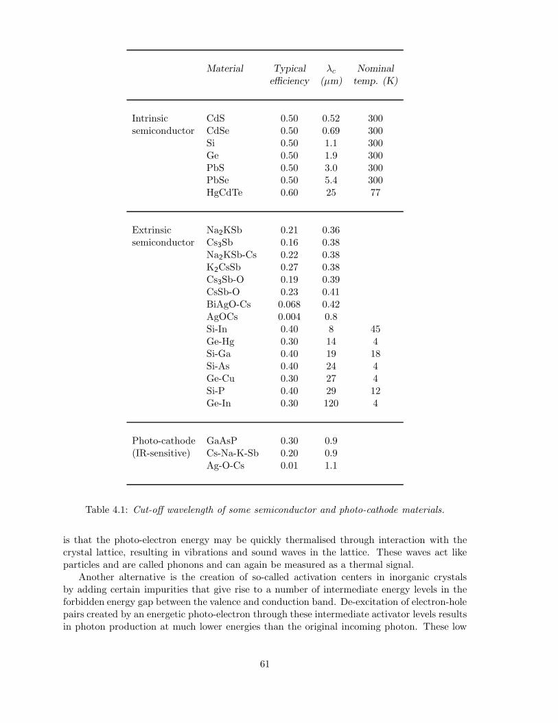
Material Typical λc Nominalefficiency (μm) temp. (K)

Intrinsic CdS 0.50 0.52 300semiconductor CdSe 0.50 0.69 300

Si 0.50 1.1 300Ge 0.50 1.9 300PbS 0.50 3.0 300PbSe 0.50 5.4 300HgCdTe 0.60 25 77

Extrinsic Na2KSb 0.21 0.36semiconductor Cs3Sb 0.16 0.38

Na2KSb-Cs 0.22 0.38K2CsSb 0.27 0.38Cs3Sb-O 0.19 0.39CsSb-O 0.23 0.41BiAgO-Cs 0.068 0.42AgOCs 0.004 0.8Si-In 0.40 8 45Ge-Hg 0.30 14 4Si-Ga 0.40 19 18Si-As 0.40 24 4Ge-Cu 0.30 27 4Si-P 0.40 29 12Ge-In 0.30 120 4

Photo-cathode GaAsP 0.30 0.9(IR-sensitive) Cs-Na-K-Sb 0.20 0.9

Ag-O-Cs 0.01 1.1

Table 4.1: Cut-off wavelength of some semiconductor and photo-cathode materials.

is that the photo-electron energy may be quickly thermalised through interaction with thecrystal lattice, resulting in vibrations and sound waves in the lattice. These waves act likeparticles and are called phonons and can again be measured as a thermal signal.

Another alternative is the creation of so-called activation centers in inorganic crystalsby adding certain impurities that give rise to a number of intermediate energy levels in theforbidden energy gap between the valence and conduction band. De-excitation of electron-holepairs created by an energetic photo-electron through these intermediate activator levels resultsin photon production at much lower energies than the original incoming photon. These low

61

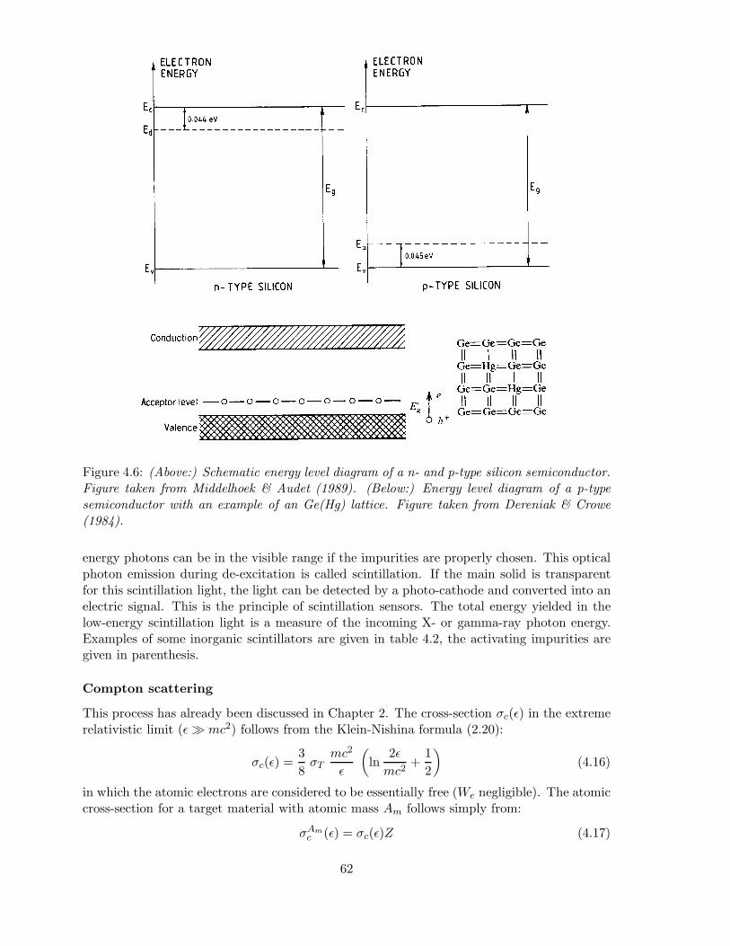
Figure 4.6: (Above:) Schematic energy level diagram of a n- and p-type silicon semiconductor.Figure taken from Middelhoek & Audet (1989). (Below:) Energy level diagram of a p-typesemiconductor with an example of an Ge(Hg) lattice. Figure taken from Dereniak & Crowe(1984).

energy photons can be in the visible range if the impurities are properly chosen. This opticalphoton emission during de-excitation is called scintillation. If the main solid is transparentfor this scintillation light, the light can be detected by a photo-cathode and converted into anelectric signal. This is the principle of scintillation sensors. The total energy yielded in thelow-energy scintillation light is a measure of the incoming X- or gamma-ray photon energy.Examples of some inorganic scintillators are given in table 4.2, the activating impurities aregiven in parenthesis.

Compton scattering

This process has already been discussed in Chapter 2. The cross-section σc(ε) in the extremerelativistic limit (ε� mc2) follows from the Klein-Nishina formula (2.20):

σc(ε) =38σT

mc2

ε

(ln

2εmc2

+12

)(4.16)

in which the atomic electrons are considered to be essentially free (We negligible). The atomiccross-section for a target material with atomic mass Am follows simply from:

σAmc (ε) = σc(ε)Z (4.17)

62

Figure 4.7: External photo-electric process. Figure taken from Dereniak & Boreman (1996).

Material Wavelength Decay Index ofof maximum constant refraction

emission (μs) at λmax

λmax (nm)

NaI(Tl) 410 0.23 1.85CsI(Na) 420 0.63 1.84CsI(Tl) 565 1.0 1.846LiI(Eu) 470 – 485 1.4 1.96ZnS(Ag) 450 0.20 2.36CaF2(Eu) 435 0.9 1.44

Table 4.2: Properties of some inorganic scintillators.

with Z the atomic number. This process is therefore proportional to Z (compare ∼ Z5 for thephoto-electric effect). Moreover, since this process is a scattering process, the full detection ofthe photon-energy requires an interaction cascade: the primary photon is successively down-scattered in energy until it is sufficiently reddened to be captured by the photo-electric effect.Figure 4.8 shows k(ε) for a few commonly used detection materials.

Pair production

Pair production is a typical quantum theoretical process. It can be envisaged as a photo-electric effect with an electron of negative energy in the Dirac-electron sea (virtual electron).

63

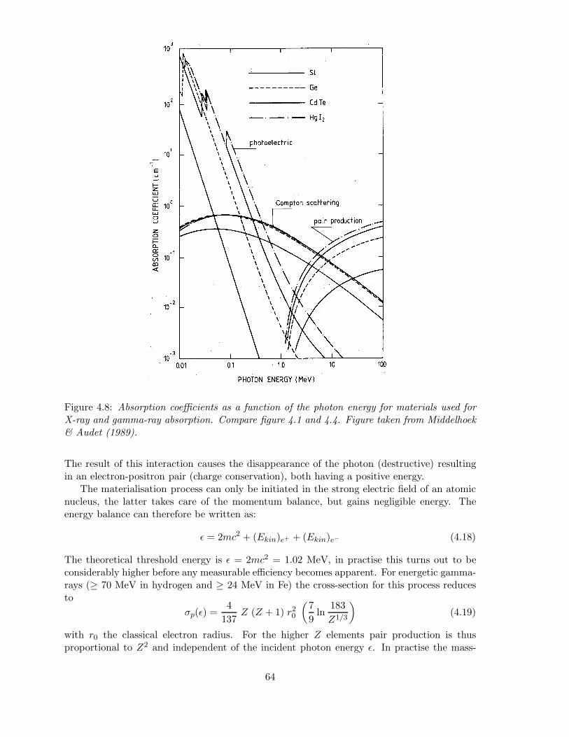
Figure 4.8: Absorption coefficients as a function of the photon energy for materials used forX-ray and gamma-ray absorption. Compare figure 4.1 and 4.4. Figure taken from Middelhoek& Audet (1989).

The result of this interaction causes the disappearance of the photon (destructive) resultingin an electron-positron pair (charge conservation), both having a positive energy.

The materialisation process can only be initiated in the strong electric field of an atomicnucleus, the latter takes care of the momentum balance, but gains negligible energy. Theenergy balance can therefore be written as:

ε = 2mc2 + (Ekin)e+ + (Ekin)e− (4.18)

The theoretical threshold energy is ε = 2mc2 = 1.02 MeV, in practise this turns out to beconsiderably higher before any measurable efficiency becomes apparent. For energetic gamma-rays (≥ 70 MeV in hydrogen and ≥ 24 MeV in Fe) the cross-section for this process reducesto

σp(ε) =4

137Z (Z + 1) r20

(79

ln183Z1/3

)(4.19)

with r0 the classical electron radius. For the higher Z elements pair production is thusproportional to Z2 and independent of the incident photon energy ε. In practise the mass-

64

Figure 4.9: The relative importance of different forms of energy loss mechanisms for γ-raysas a function of photon energy and atomic number. Figure taken from Hillier (1984) andLongair (1992).

absorption coefficient is always used:

κp(ε) =NA

Am(σp(ε) =

79X−1

0 (4.20)

with

X0 =(

4137

NA

AmZ (Z + 1) r20 ln

183Z1/3

)−1

(4.21)

As can be seen from this equation, X0 only depends on the material properties under consid-eration and not on the photon energy ε. X0 is called the radiation length in units of kg·m−2,and is a standard parameter in high-energy γ-ray astrophysics. It really is a mass absorptioncoefficient with the same units as a surface density, but after multiplication with the densityit becomes a length scale.

The radiation length is then used to characterise the absorbing medium: the attenuationis given by:

I(x) = I(0) exp(−7

9x

X0

)(4.22)

Numerical values for largely different Z are

X0 � 6 g·cm−2 −→ 5.3 mm for a lead slabX0 � 62 g·cm−2 −→ 7 km for hydrogen at 1 bar

Figure 4.9 summarizes the relative importance of the three major types of photo-electricradiation absorption. The solid lines show the values of Z and ε for which the two neighboringeffects are just equal.

65

Figure 4.10: Theoretical solar neutrino spectrum. Figure taken from Kitchen (1991).

Reflection and refraction

In the previous sections the physical principles of thermal and photo-electric absorption havebeen described. If a radiation beam arrives at the interface between two media with refractiveindices ni and nt, Fresnel’s laws apply giving the relation between the intensity of the incident,the reflected and the transmitted (=refracted) beam. This is relevant for low energy photonsand plays an important role in the overall efficiency of the detection process since reflectionlosses at the interface may be substantial. Since Fresnel’s laws are extensively treated in anystandard textbook on optics, this subject will not be elaborated in this course.

4.3 Neutrino detection

The mean free path for neutrino detection

λ(εν) =1

σ(εν)N(4.23)

is extremely long due to the exceedingly small value of the nuclear cross-section σ(εν) for theinteraction process. For the highest electron-neutrino energies, σ(ενe) for capture in chlorineamounts to ≈ 10−46 m2, yielding a λ ≈ 1 parsec in pure 37

17Cl.

66

The neutrino capture reaction in chlorine can be written as:

νe + 3717Cl −→ 37

18Ar + e− (4.24)

The threshold energy for this reaction to occur is ενe = 0.814 MeV. This is greater than themaximum energy of the electron neutrinos generated in the main p-p chain in stellar interiors,but smaller than that of those produced in the decay of 8B, see figure 4.10.

In the deep mine of the Home-state Gold Mining Company (South Dakota), the radio-active 37Ar is generated in about 600 tons of perchloro-ethylene C2Cl4. The incoming electronneutrinos release the 37Ar from the molecule and they can be flushed out of the fluid bypassing He through the volume. The 37Ar decays with a half life of 34.8 days by capturingone of the inner orbital electrons (electron capture, EC). The photon which is released by thisprocess is used to expel one of the outer electrons and ionise the atom. This free electron iscalled the Auger electron and has a fixed energy of 2.82 keV:

3718Ar + EC −→ 37

17Cl+ + e− (2.82keV) (4.25)

This low-energy electron is detected in a sensitive gas proportional counter.The Kamiokande experiment (Mitsui Mining Company in Japan) uses an active volume

of 3000 tons of very pure water. The neutrino produces an energetic electron by scattering:

νx + e −→ ν ′x + e′ (4.26)

This electron will move with a speed greater than the local speed of light. Due to the abruptchange of the electric field the surrounding atoms will emit radiation. This so-called Cerenkovradiation can be detected and also provides some directionality information due to the forwardbeaming of the cone of Cerenkov emission. As indicated with νx, this technique has also somesensitivity for the detection of νμ and ντ . The scattering probabilities are:

ps(νμ) ≈ ps(ντ ) ≈ 17ps(νe) (4.27)

Two other large neutrino experiments entail the SAGE (Soviet-American Gallium Ex-periment) and the GALLEX (Gallium Experiment) located in the Gran Sasso UndergroundLaboratory in the Italian Appennino Mountains, which comprises a collaboration betweenEurope, the United States and Israel. These experiments make use of the reaction:

νe + 7131Ga −→ 71

32Ge + e− (4.28)

The threshold energy for this reaction is approximately 0.233 MeV which allows the large fluxof low energy neutrinos emitted in the p-p process to be detected.

GALLEX employs 30 tonnes of gallium used in an aqueous solution of gallium chlorideand hydrochloric acid. The 71Ge decays with a half lifetime of 11.4 days by electron capture:

7132Ge + EC −→ 71

31Ga+ + e− (10.37 keV) (4.29)

The Auger electron is again measured in a sensitive gas-filled radiation sensor.SAGE uses 60 tonnes of solid gallium, located in the Caucasus mountains (Baksan Valley).

Heating melts the gallium and flushing with hydrochloric acid brings out the volatile GeCl4.No firm results are yet available.

67

Both the Kamiokande experiment in Japan and the IMB detector in theUnited States have seen a neutrino pulse from the supernova explosion inthe Large Magellanic Cloud SN1987A on February 23th, 1987. Duringthe collapse of the core of the progenitor star, about 1058 neutrinos wereemitted. Of these neutrinos 20 were detected in the water detectorsmentioned above, see figure below. Precisely on that day there wereproblems with the Japanese electricity net, due to which the clocks werenot completely synchronised with Universal Time. Hence, the arrivaltimes of the neutrinos detected with Kamiokande have an uncertaintyof about 60 seconds.The IMB detected the first neutrinos at 07:35:41. At 09:22 Jones did notobserve any new star, at 10:38 the first optical picture of the supernovawas made by Garrad and McNaught, but they did not develop their filmimmediately. Only in the following night Shelton and Duhalde were thefirst to see a supernova in 383 years with their naked eye.

An important recent development has been the completion and operation of the SudburyNeutrino Observatory (SNO)in Ontario, Canada. This neutrino detector has been built twokilometers underground, the detection principle is based on neutrino interaction with theDeuterium nucleus in heavy water. Three reactions are possible:

νe + 21H −→ p + p + e− (4.30)

νx + 21H −→ p + n + νx (4.31)

νx + e− −→ νx + e− (4.32)

The neutrino absorption in the first reaction only applies to electron-neutrino’s, the other reac-tions, i.e. the deuteron break-up and energetic electron scatter respectivily, apply to any typeof neutrino (νx). In the deuteron break-up reaction, the nucleus splits into its constituent

68

Figure 4.11: Energy loss rate due to ionisation losses for cosmic-ray particles. Figure takenfrom Longair (1992).

components, i.e. a proton and a neutron, the neutron eventually recombines with anotherdeuteron, releasing a gamma-ray photon that , in turn, knocks-on an energetic electron. Theenergetic electrons are all detected by the emission of Cerenkov light. The deuteron break-upreaction measures the total flux of all neutrino flavours above a threshold energy of ≈ 2.2MeV, consequently the detector is sensitive to the 8B solar neutrino flux (see figure 4.10).The detector comprises a volume of 1000 tons of heavy water, viewed by more than 9500 pho-tomultiplier tubes, held on an 18-meter geodesic sphere, that measure the emitted Cerenkovlight cones. The different reactions can be separated by the different energy distributions andemission geometries of the energetic electrons. Recently, 2 kilotons of NaCl (salt) was addedto enhance the efficiency of neutron-capture after the deuteron break-up reaction.The most recent results of this instrument have convincingly demonstrated that solar neu-trino’s indeed change ”flavour” on there journey from the solar interior to the earth, i.e. thatphase transitions occur between νe, νμ and ντ neutrino’s. This is not in agreement with ”thestandard model” in physics, and implies that neutrino’s have at least some mass. This resultalso solves the almost 30 years standing problem of the so-called deficit in the solar neutrinoflux, namely that the number of electron neutrino’s observed appeared to be only one-thirdto one-half of the flux computed on the basis of standard stellar nuclear fusion models.The estimated flux density of electron neutrino’s is (1.59 ± 0.08) 106 cm−2s−1, the total neu-trino flux density amounts to (5.21 ± 0.27) 106 cm−2s−1. The latter value is very close to theflux density derived from current models of stellar evolution.

4.4 Cosmic-ray detection

Cosmic-ray particles lose energy by ionisation when traversing matter. The ionisation lossper unit path-length is given by relativistic quantum theory and is known as the Bethe-Blochformula:

−dEdx

= −dEkin

dx=

Z2q4nZ0

4πε20mev2

[ln

(2γ2mev

2

I

)− v2

c2

]= Z2nZ0f(v) (4.33)

69

Figure 4.12: Stopping power per unit mass length in various materials as a function of theLorentz factor γ, kinetic energy and momentum (inset). Figure taken from Longair (1992).

with Zq the charge of the cosmic-ray particle under consideration, n the atomic density of thetarget material, Z0 its atomic number, I the average ionisation potential and v the particlevelocity. The formula indicates that the energy loss depends only on the velocity of theparticle and on its charge, given a medium characterised by nZ0. The velocity (or energy)dependence is shown in figure 4.11. Up to velocity v ≈ c or kinetic energy Ekin ≈ Ammpc

2

the ionisation loss decreases as v−2 or E−1kin. For energies around Ammpc

2 there is a minimumin the ionisation loss: a particle with this kinetic energy is designated as a minimum ionisingparticle. At higher energies the ionisation loss slowly increases again proportional to ln(γ2).

The quantity dE/dx is often referred to as the stopping power of the material. This powercan also be expressed in terms of the mass per unit area traversed by the cosmic-ray particle(equivalent to the mass-absorption coefficient for electromagnetic radiation κ(ε). With ξ = ρx(in kg m−2):

−dEkin

dξ= −dEkin

dx

dx

dξ=

1nA0mp

Z2nZ0f(v) = Z2f(v)Z0

A0mp(4.34)

The ratio Z0/A0mp is rather insensitive to Z for all stable elements, it varies from 1/(2mp)for light elements to 1/(2.4mp) for uranium. Thus, the only variation of the energy loss fromelement to element is the variation in I. Figure 4.12 shows −dE/dξ as a function of kineticenergy per nucleon (expressed in terms of γ−1, see equation 2.59) for singly charged (protonsand electrons) and doubly charged (He-nuclei) particles for several target materials. Despitethe wide range of values of I for those materials, it can be seen that the curves lie remarkablyclose together for singly charged particles, this is due to the logarithmic dependence on I. Thismeans that the quantity (dEkin/dξ)/Z2 is almost constant and if the energy loss dEkin/dξis measured as a function of the kinetic energy Ekin of the particle, the charge Z (the onlyvariable left) can be measured. Moreover, the minimum ionisation loss occurs at a Lorentz-factor γ ≈ 2 and can be well approximated for any species by 0.2Z2 MeV (kg m−2)−1. If thisenergy loss is measured the relativistic movement of the particle is ascertained.

70

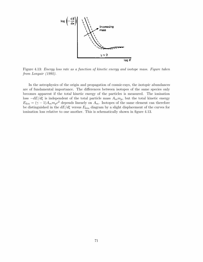
Figure 4.13: Energy loss rate as a function of kinetic energy and isotope mass. Figure takenfrom Longair (1992).

In the astrophysics of the origin and propagation of cosmic-rays, the isotopic abundancesare of fundamental importance. The differences between isotopes of the same species onlybecomes apparent if the total kinetic energy of the particles is measured. The ionisationloss −dE/dξ is independent of the total particle mass Ammp, but the total kinetic energyEkin = (γ − 1)Ammpc

2 depends linearly on Am. Isotopes of the same element can thereforebe distinguished in the dE/dξ versus Ekin diagram by a slight displacement of the curves forionisation loss relative to one another. This is schematically shown in figure 4.13.

71

Chapter 5

Characterization of instrumentalresponse

5.1 Characteristic parameters

Characterization of the performance and response of a physical measurement system canbe achieved by considering a multidimensional parameter space, in which each coordinateaxis relates to a specific instrument parameter that has a major influence on the quality ofthe measurement. For astrophysical observations these parameters comprise, among others,bandwidth, field of view, precision and resolution, limiting sensitivity.

In the following paragraphs a brief description of these parameters is given. It should bekept in mind, however, that a certain “bandwidth” in the definitions of these parameters isinevitable and due account must be taken of their exact meaning in a particular observationalcontext.

5.1.1 Bandwidth (symbol: λλ, νν, or εε)

The bandwidth, or rather spectral bandwidth, is defined as the wavelength (or frequency, orenergy) interval over which the instrument has adequate detection efficiency, i.e. over whichit is observationally employed. The long and short wavelength cut-offs are derived fromthe wavelength dependent detection efficiency, which is governed by the physical interactionprocess (see chapter 4). The precise criteria for choosing the cut-off values are mostly ratherarbitrary, e.g. cut-off is defined at 50 % or 10 % of the value of maximum efficiency in thebandpass.

5.1.2 Field of view (FOV, symbol: ΩFOV )

The field of view is defined as the solid angle subtended on the sky by the selected telescopeconfiguration. If the effective area of the telescope is a continuously declining function of theoff-axis (optical axis) angle, the choice of the effective FOV is somewhat arbitrary (like in thecase of spectral bandwidth), e.g. decline to half the maximum sensitive area (FOV at FullWidth at Half Maximum (FWHM)) or to zero sensitive area (FOV at Full Width at ZeroResponse (FWZR)). The effective FOV is also dependent on the angular resolution which isrequired for an observation: due to the potential decline of the image quality with off-axisangle not the whole field of view may qualify for a particular observation.

72

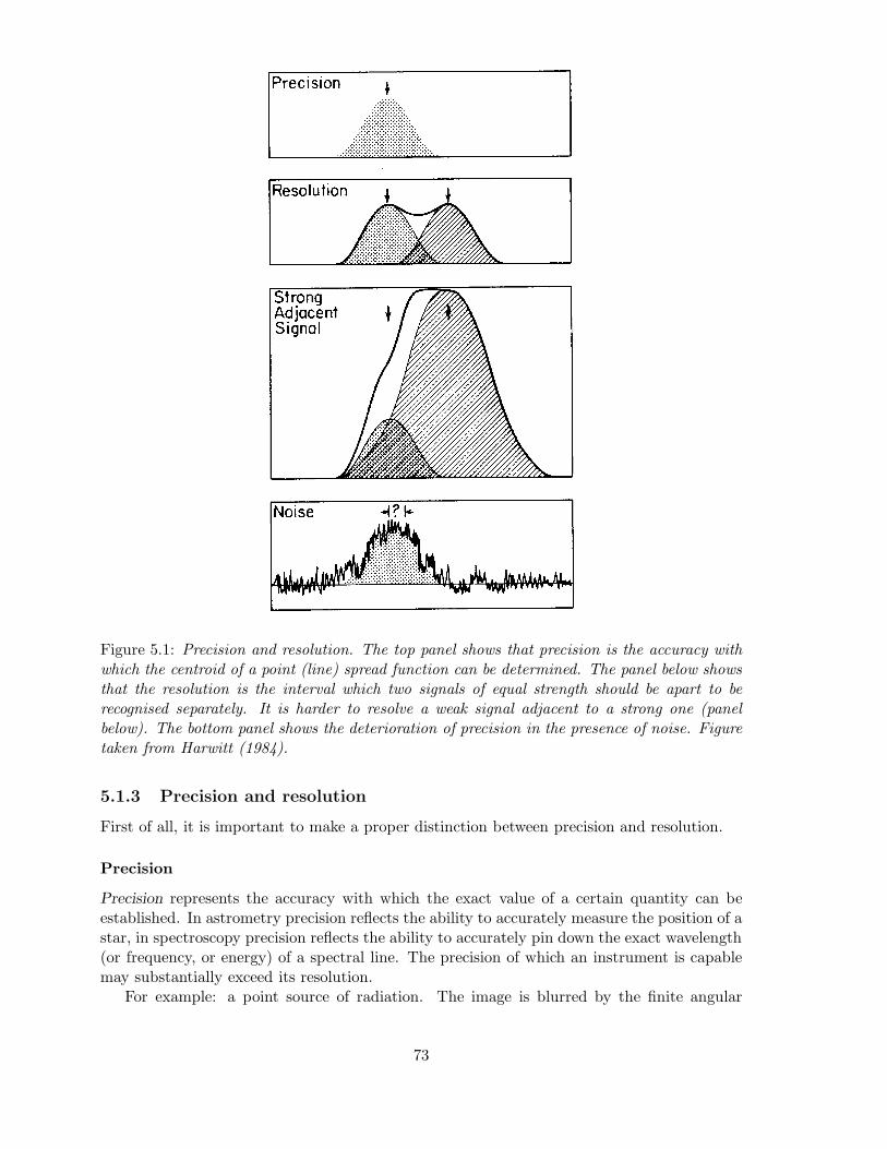
Figure 5.1: Precision and resolution. The top panel shows that precision is the accuracy withwhich the centroid of a point (line) spread function can be determined. The panel below showsthat the resolution is the interval which two signals of equal strength should be apart to berecognised separately. It is harder to resolve a weak signal adjacent to a strong one (panelbelow). The bottom panel shows the deterioration of precision in the presence of noise. Figuretaken from Harwitt (1984).

5.1.3 Precision and resolution

First of all, it is important to make a proper distinction between precision and resolution.

Precision

Precision represents the accuracy with which the exact value of a certain quantity can beestablished. In astrometry precision reflects the ability to accurately measure the position of astar, in spectroscopy precision reflects the ability to accurately pin down the exact wavelength(or frequency, or energy) of a spectral line. The precision of which an instrument is capablemay substantially exceed its resolution.

For example: a point source of radiation. The image is blurred by the finite angular

73

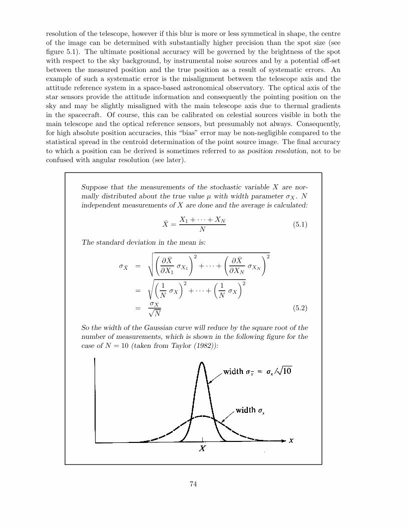
resolution of the telescope, however if this blur is more or less symmetical in shape, the centreof the image can be determined with substantially higher precision than the spot size (seefigure 5.1). The ultimate positional accuracy will be governed by the brightness of the spotwith respect to the sky background, by instrumental noise sources and by a potential off-setbetween the measured position and the true position as a result of systematic errors. Anexample of such a systematic error is the misalignment between the telescope axis and theattitude reference system in a space-based astronomical observatory. The optical axis of thestar sensors provide the attitude information and consequently the pointing position on thesky and may be slightly misaligned with the main telescope axis due to thermal gradientsin the spacecraft. Of course, this can be calibrated on celestial sources visible in both themain telescope and the optical reference sensors, but presumably not always. Consequently,for high absolute position accuracies, this “bias” error may be non-negligible compared to thestatistical spread in the centroid determination of the point source image. The final accuracyto which a position can be derived is sometimes referred to as position resolution, not to beconfused with angular resolution (see later).

Suppose that the measurements of the stochastic variable X are nor-mally distributed about the true value μ with width parameter σX . Nindependent measurements of X are done and the average is calculated:

X =X1 + · · · +XN

N(5.1)

The standard deviation in the mean is:

σX =

√√√√( ∂X∂X1

σX1

)2

+ · · · +(∂X

∂XNσXN

)2

=

√(1NσX

)2

+ · · · +(

1N

σX

)2

=σX√N

(5.2)

So the width of the Gaussian curve will reduce by the square root of thenumber of measurements, which is shown in the following figure for thecase of N = 10 (taken from Taylor (1982)):

74

Another example is the timing precision (symbol: Δtabs = tabs− tobservatory), which equalsthe difference between the measured time and true time. The absolute timing accuracy is par-ticularly important for synchronisation of periodic phenomena over time series with repeatedinterupts (satellite data) or over different observations. For example in pulsar observations,the period of a pulsar (and other parameters like period derivative or orbital period and or-bital period derivative in case of a binary) can be determined to a much higher precision,when two observations at different times are synchronised: i.e. the exact number of pulseperiods between the two observations should be known. From the time of arrival of the pulseat the first observation and the predicted period (and period derivative etc.) a prediction ismade of the time of arrival of the pulses in the second observation. From the deviation ofthe measured time of arrival a better value of the period (and period derivative etc.) can bedetermined. (The absolute time of an observation is usually determined by comparing theobservatory maser clock with a GPS system (Global Positioning System) which is locked toUniveral Time (UT) determined by the world’s best atomic clocks.)

Resolution

Resolution (or resolving power) represents the capability of measuring the separation betweentwo closely spaced features, e.g. two spectral lines or two point like radiation sources. Thefollowing resolutions are commonly used in astrophysical data:

• Angular resolution (symbol: Δθ)This is defined as the minimum angular separation needed between two equally brightpoint sources to ensure that they can be individually just separated (“resolved”).

If an angle of Δθ radians can just be resolved, the angular resolving power is

Rθ =1

Δθ(5.3)

• Spectral resolution (symbol: Δλ,Δν or Δε)This is defined as the separation in wavelength (or frequency, or energy) between twospectral lines of equal intensity, that is just large enough to resolve the lines individually.

The spectral resolving power is the ratio of the wavelength λ at which the observationis carried out, to the wavelength difference Δλ which can just be resolved:

RS =λ

Δλ=

ν

Δν=

ε

Δε(5.4)

• Charge and mass resolution (symbol: ΔZ and ΔA)These characteristic parameters are relevant for the measurement of the composition ofa particle beam (e.g. cosmic-rays). It is defined as the fractional charge and mass whichcan just be separated by a particle telescope.

The charge and mass resolving power is the ratio of the charge Z, mass A, which isbeing measured, to the charge difference ΔZ, mass difference ΔA, which can be justresolved:

RZ =Z

ΔZ(5.5)

RA =A

ΔA(5.6)

75

• Temporal resolution (symbol: Δt)This parameter can be defined as representing the minimum time interval between twoconsecutive samples of a realisation of a stochastic process for which these samples canbe regarded as uncorrelated (independent) at the output of the measuring device.

It is important to realise that the characteristic resolution parameters defined above, applyto closely spaced features of comparable strength. If, for instance, a faint star lies very closeto a brighter companion, or a faint spectral line lies near a far brighter spectral feature, thetwo may not be separable with a given resolution, even though a pair of equally bright starsor spectral lines would be easily resolved at the same separation.

5.1.4 Limiting sensitivity [symbol: (F (λ, ν, ε)min]

The limiting sensitivity achievable with a specific observation facility is defined as the min-imum value of the monochromatic flux density arising from a celestial point source, thatcan be detected significantly over a certain measuring period T in a predefined wavelength(frequency, energy) interval.

This parameter is a function of the effective telescope area Aeff , integration time T andangular resolution Δθ, moreover it may strongly depend on sky position (background light)and instrumental noise (potentially variable). If the nature of the radiation source is truelydiffuse in origin, like a cosmic-ray beam incident on a particle telescope, the collecting power ofthe instrument is normally related to the so-called geometry factor or grasp. This parameteris defined as the telescope effective area integrated over the FOV of the telescope:

GF =∫ΩF OV

Aeff dΩ (5.7)

Derivation of expressions for the limiting sensitivity will be discussed in some detail in chapter6.

5.1.5 Polarisation sensitivity (symbol: Πmin)

The information carried by the polarisation of electromagnetic radiation is important, sinceit characterizes the physical conditions of the emission region. The polarisation is defined byusing four so-called Stokes parameters. The detection system may only be sensitive to onepolarisation component (such as a radio dipole antenna) and the telescope (optics, waveguides)may potentially alter it. The polarisation sensitivity is therefore defined as the accuracy towhich the Stokes parameters can be measured.

76

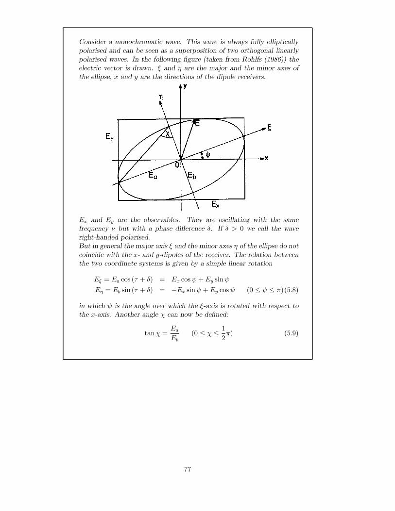
Consider a monochromatic wave. This wave is always fully ellipticallypolarised and can be seen as a superposition of two orthogonal linearlypolarised waves. In the following figure (taken from Rohlfs (1986)) theelectric vector is drawn. ξ and η are the major and the minor axes ofthe ellipse, x and y are the directions of the dipole receivers.

Ex and Ey are the observables. They are oscillating with the samefrequency ν but with a phase difference δ. If δ > 0 we call the waveright-handed polarised.But in general the major axis ξ and the minor axes η of the ellipse do notcoincide with the x- and y-dipoles of the receiver. The relation betweenthe two coordinate systems is given by a simple linear rotation

Eξ = Ea cos (τ + δ) = Ex cosψ +Ey sinψEη = Eb sin (τ + δ) = −Ex sinψ + Ey cosψ (0 ≤ ψ ≤ π)(5.8)

in which ψ is the angle over which the ξ-axis is rotated with respect tothe x-axis. Another angle χ can now be defined:

tanχ =Ea

Eb(0 ≤ χ ≤ 1

2π) (5.9)

77

In 1892 Poincare showed that there exists a one-to-one relation betweenpolarisation states of a wave and points on a sphere with radius E2

a +E2b .

The angles 2ψ and 2χ can be seen as the longitude and the lattitude ofthe sphere. The three coordinates of each point are the Stokes param-eters Q, U and V , see the following figure (taken from Rohlfs (1986)).

Points on the equator represents linear polarised waves (V = 0), thenorth pole represents a right-circular polarised wave and the south polea left-circular. The Stokes parameters are defined as

I = E2a + E2

b (5.10)Q = I cos 2ψ cos 2χ (5.11)U = I sin 2ψ cos 2χ (5.12)V = I sin 2χ (5.13)

By definition a monochromatic wave is fully polarised:

I2 = Q2 + U2 + V 2 (5.14)

Now the Stokes parameters can be expressed in the observable parame-ters E1, E2 and δ:

I = E21 + E2

2 (5.15)Q = E2

1 − E22 (5.16)

U = 2E1E2 cos δ (5.17)V = 2E1E2 sin δ (5.18)

5.2 Convolutions

5.2.1 General

In the preceeding paragraph several characteristic parameters have been defined which relateto the resolution of the astrophysical instrumentation in use. Although this gives a handle oncapability and potential performance, for quantitative handling of the data full account needs

78

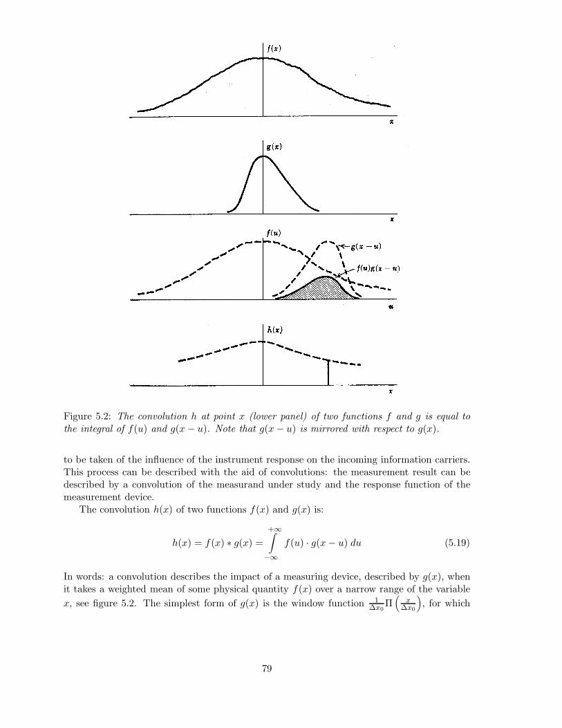
Figure 5.2: The convolution h at point x (lower panel) of two functions f and g is equal tothe integral of f(u) and g(x− u). Note that g(x− u) is mirrored with respect to g(x).

to be taken of the influence of the instrument response on the incoming information carriers.This process can be described with the aid of convolutions: the measurement result can bedescribed by a convolution of the measurand under study and the response function of themeasurement device.

The convolution h(x) of two functions f(x) and g(x) is:

h(x) = f(x) ∗ g(x) =+∞∫

−∞f(u) · g(x− u) du (5.19)

In words: a convolution describes the impact of a measuring device, described by g(x), whenit takes a weighted mean of some physical quantity f(x) over a narrow range of the variablex, see figure 5.2. The simplest form of g(x) is the window function 1

Δx0Π(

xΔx0

), for which

79

the convolution integral reduces to the expression for the so-called running average:

1Δx0

+∞∫−∞

f(u)Π(x− u

Δx0

)du =

1Δx0

x+ 12x0∫

x− 12x0

f(u)du (5.20)

Convolutions are commutative, associative and distributive, i.e.:

f(x) ∗ g(x) = g(x) ∗ f(x) (5.21)f(x) ∗ (g(x) ∗ h(x)) = (f(x) ∗ g(x)) ∗ h(x) (5.22)f(x) ∗ (g(x) + h(x)) = f(x) ∗ g(x) + f(x) ∗ h(x) (5.23)

5.2.2 Fourier transforms

Convolutions can be easily and elegantly handled by employing the Fourier transform tech-nique. The Fourier transform of a function g(x) exists if it satisfies the following conditions:

1. The integral of |g(x) | exists, i.e.∫∞−∞ |g(x) | dx is convergent.

2. Discontinuities in g(x) are finite.

The Fourier transform F(g(x)) of g(x) is called G and is a function of the Fourier domainvariable s:

F(g(x)) = G(s) =+∞∫

−∞g(x) e−2πisx dx (5.24)

The inverse transform is given by

g(x) =+∞∫

−∞G(s) e2πisx ds (5.25)

For a function h(t) depending on time, its Fourier transform will depend on the frequencyvariable f :

H(f) =+∞∫

−∞h(t) e−2πift dt (5.26)

Sometimes the frequency variable f is replaced by the angular frequency ω = 2πf , yielding

H(ω) =+∞∫

−∞h(t) e−iωt dt (5.27)

h(t) =12π

+∞∫−∞

H(ω) eiωt dω (5.28)

which lacks the symmetry of the expressions in f .A Fourier transform pair is often indicated in a symbolic way by a double arrow: g(x) ⇔

G(s) or h(t) ⇔ H(f).

80

A particular useful theorem from Fourier theory states that the Fourier transform of theconvolution of two functions equals the product of the Fourier transforms of the individualfunctions

F(f ∗ g) = F(f) · F(g) or, in shorthand : f ∗ g ⇔ F (s) ·G(s) (5.29)

This is called the convolution theorem. Other useful and frequently applied theorems are

f(ax) ⇔ 1|a | F

(s

a

)(5.30)

f(x) + g(x) ⇔ F (s) +G(s) (5.31)f(x− a) ⇔ e−2πiasF (s) Shift theorem (5.32)

f(x) cosωx ⇔ 12F

(s− ω

2π

)+

12F

(s+

ω

2π

)(5.33)

f(x) ∗ f∗(−x) ⇔ |F (s) |2 (5.34)f ′(x) ⇔ 2πis F (s) (5.35)

d

dx(f(x) ∗ g(x)) = f ′(x) ∗ g(x) = f(x) ∗ g′(x) (5.36)

+∞∫−∞

|f(x) |2 dx =+∞∫

−∞|F (s) |2 ds Parseval’s theorem (5.37)

+∞∫−∞

f(x)g∗(x) dx =+∞∫

−∞F (s)G∗(s) ds (5.38)

f and g real

+∞∫−∞

f(x)g(−x) dx =+∞∫

−∞F (s)G(s) ds (5.39)

5.3 Instrument response and data sampling

5.3.1 Response fuctions

In observational astrophysics it is often necessary to have a full and quantitative knowlegdeof the angular and spectral reponse functions in order to perform a proper deconvolution ofthe measurement data to extract optimally the characteristics of the information source.

Consider the example of a spectrometer which possesses a response function R(λ, λ′). Inmany cases, the smearing effect (or blurring) of the spectrometer is solely a function of thewavelength difference λ′ − λ, i.e. R(λ, λ′) = R(λ′ − λ). If the information source emits aspectrum S(λ), the source function, the measured distribution M(λ) at the output of thespectrometer is given by the convolution:

M(λ) =+∞∫

−∞S(λ′)R(λ− λ′) dλ′ =

∞∫0

S(λ′)R(λ− λ′) dλ′ (5.40)

since S(λ) = 0 for λ ≤ 0. Applying the convolution theorem, with S(λ) ⇔ S(s), R(λ) ⇔ R(s)and M(λ) ⇔M(s)

S(s) =M(s)R(s)

(5.41)

81

The spectrum of the source can be reconstructed by deconvolution of the measured spectrum.This is accomplished through the inverse Fourier transform:

S(λ) = F−1[M(s)R(s)

](5.42)

To illustrate the notions just described, consider a spectrometer with a Gaussian responsefunction:

R(λ) =1√2πσ

e−λ2

2σ2 (5.43)

Suppose an infinitely narrow spectral line at wavelength λ0 is measured: S(λ) = S0 ·δ(λ−λ0).The convolution of S(λ) and R(λ) gives the measured result, which is (of course) a Gaussiandistributed profile around λ0:

M(λ) =S0√2πσ

e−(λ−λ0)2

2σ2 (5.44)

Suppose an observer has measured M(λ) and R(λ) is known. He can now reconstruct S(λ).First the Fourier transform of M(λ) is taken:

M(s) =+∞∫

−∞M(λ) e−2πisλ dλ

=+∞∫

−∞

S0√2πσ

e−(λ−λ0)2

2σ2 e−2πisλ dλ

=S0√2πσ

e−2πisλ0−2π2s2σ2

+∞∫−∞

e−(λ−λ0)2

2σ2 −2πis(λ−λ0)+2π2σ2s2

dλ

=S0√2πσ

e−2πisλ0−2π2s2σ2

+∞∫−∞

e−πλ′2√2πσ dλ′

= S0 e−2πisλ0−2π2s2σ2

(5.45)

where λ′ = λ−λ0√2πσ

+ i√

2πσs. Analogously

R(s) = e−2π2s2σ2(5.46)

(Note that the Fourier transform of a Gaussian function is again Gaussian.) Applying equation5.42 gives

S(λ) = F−1[S0 e−2πisλ0 ] = S0 · δ(λ − λ0) (5.47)

i.e. the observer has recovered the exact form of the spectral source function.Consider now a spectrometer with a Gaussian response function with width σ. If σ is

large, i.e. the line spread function is wide, the Fourier domain only contains low frequenciesas can be seen from equation 5.46 and figure 5.3. By decreasing σ, the range of frequencies inthe Fourier domain increases and consequently the range of spectral frequencies over whichthe measurement provides information. The lnR(s) is a parabola, which tends to a δ-functionfor the limit σ → ∞ (no spectral resolution) and becomes flat for σ ↓ 0 (perfect transmissionat all frequencies).Obtaining S(λ) by this method is, in practise, complicated by two factors: data sampling andnoise. This will be adressed in the following paragraphs.

82

Figure 5.3: The line S(λ) is widened by the response function R(λ). For a broad (narrow)response the Fourier transform of the measured function M(s) contains information over anarrow (broad) range of frequencies.

5.3.2 Discrete measurement intervals, the Nyquist criterion

First of all the measurement distribution M(λ) is not a continuous function as assumed inequation 5.40, but is always sampled in discrete intervals or bins and is also not available overthe whole interval from −∞ to ∞.The problem of discrete intervals can be overcome by using the discrete version of the Fouriertransform.Suppose there are N consecutive sampled values g(xk) with xk = kτ (k = 0, 1, 2, ..., N − 1),the sampling interval is τ . With N input numbers, evidently no more than N independentoutput numbers can be produced. Estimates of the Fourier transform G(s) can now be soughtat discrete frequency values sn = n

Nτ (n = −N/2, ..., N/2). The extreme values of ncorrespond in this case to the lower and upper limits of the Nyquist critical frequency (seelater in this paragraph). Notice that in this case n takes N + 1 rather than N values, this isbecause the two extreme values of n are not independent (i.e. they are equal), this reducesthe count of independent numbers to N .

G(sn) =+∞∫

−∞g(x) e−2πisnxdx ≈

N−1∑k=0

g(xk) e−2πisnxk τ = GD(sn) (5.48)

Substitution of xk and sn yields:

GD(sn) = τN−1∑k=0

g(xk) e−2πikn/N (5.49)

where GD(sn) is the nth value of the discrete transform of g(x).The inverse Fourier tranform, which recovers the set of sampled g(xk) values exactly fromGD(sn) is given by:

g(xk) =1N

N−1∑n=0

GD(sn) e2πikn/N (5.50)

N.B. Outside the measurement range the function values are set to zero.Using discrete Fourier transforms instead of continuous transforms does not lead to loss of

83

information, provided the interval between sampling points or the bin width τ satisfies theNyquist criterion for optimum sampling. This can be qualitativily understood in the follow-ing way. Any physical measurement system has a finite frequency response, therefore themeasured distribution M(x), constituting some function of a parameter x, is contained inbandwidth, i.e. the Fourier transform M(s) ⇔M(x) is a bandlimited function, characterizedby a maximum cut-off frequency smax, also called the critical scr or Nyquist frequency. Inthe case of ’Gaussian’ response for instance: the frequencies will never be distributed purelyGaussian since no physical system transmits the tail frequencies up to ∞.Nyquist (and Shannon) established a theorem for optimum sampling of bandlimited observa-tions. This theorem states that no information is lost if sampling occurs at intervals (or inbins) τ = 1

2scr. The formal derivation of this theorem will not be given here, it is treated in

the follow-on course OAF2. Thus, the use of the discrete Fourier transform causes no lossof information, provided that the sampling frequency 1

τ is twice the highest frequency in thecontinuous input function (i.e. the source function convolved with the response function). Themaximum frequency smax that can be determined for a given sampling interval equals there-fore 1

2τ . If the input signal is sampled too slowly, i.e. if the signal contains frequencies higherthan 1

2τ , then these cannot be determined after the sampling process and the finer details willbe lost. More seriously however, the higher frequencies which are not resolved will beat withthe measured frequencies and produce spurious components in the frequency domain belowthe Nyquist frequency. This effect is known as aliasing and may give rise to major problemsand uncertainties in the determination of the source function.

Example: Consider again the above spectrometer with the Gaussianresponse function. What is the proper sampling interval for the mea-sured function M(λ)?As stated before: no physical system transmits the tail frequencies up to∞. Suppose that the frequencies of the Gaussian shaped Fourier trans-form R(s) = e−2π2σ2s2

are covered out to three standard deviations inthe s domain, i.e. the exponent 2π2σ2s2cr equals 9

2 so that scr ≈ 12σ . As

is clear from the right panel in the figure in section 5.3.1, the powerin the Fourier domain above this value of scr can be neglected. TheNyquist frequency scr = 1

2σ can be considered as appropriate and sincescr = 1

2τ the proper sampling interval τ (or bin width) for M(λ) in caseof a Gaussian line spread function with width σ is:

τ = σ (5.51)

If sampling (binning) is performed at a higher frequency the informa-tion in M(λ) is oversampled, at lower frequencies undersampled. It isimportant to note that although oversampling ensures the transfer ofall information, it also leads to statistical dependence between adjacentpoints (bins). This implies that standard statistical tests, like the χ2-test or other likelihood tests, do not apply anymore since they assumestatistically independent samples.

5.3.3 Noise

Secondly the presence of noise (both intrinsic to the signal and background noise) and distur-bances will produce ambiguities in the values derived for S(λ). Handling the errors and their

84

Figure 5.4: Operation that defines the Wiener filter problem

propagation is a major subject in deconvolution processing to arrive at reliable confidenceintervals for the physical parameters estimated for the radiation source. Sophisticated filteralgorithms have been developed to optimally reduce the influence of noise. Random noise canbe most efficiently reduced by employing so-called optimal or Wiener filters. If applied to astochastic process, the Wiener filter is the optimum result if the filter is designed such thatits output is a good estimate of either the past, the present or the future value of the inputsignal. The basic problem to be addressed is depicted in figure 5.4. The input signal W (t) isa stochastic process comprising the sum of a signal component X(t) and a noise componentN(t):

W (t) = X(t) + N(t) (5.52)

The system is assumed to be linear with a tranfer function H(f), being the Fourier transformof the impulse response function h(t). The output of the system is denoted Y (t).In general , H(f) is selected such that Y (t) is the best possible estimate of the input signalX(t) at the time t+ t0, that is the best estimate of X(t+ t0). If t0 > 0, Y (t) is an estimateof a future value of X(t) corresponding to a prediction filter. If t0 < 0, Y (t) is an estimate ofthe past value of X(t), corresponding to a smoothing filter. If t = 0, Y (t) is an estimate of thecurrent value of X(t).If Y (t) differs from the desired true value of X(t+ t0), the error is:

ε(t) = X(t+ t0) − Y (t) (5.53)

This error is illustrated conceptually in figure 5.4 by dashed lines. The optimum filter will bechosen so as to minimize the mean-squared value of ε(t):

minimize E{ε2(t)

}= E

{[X(t+ t0) − Y (t)]2

}(5.54)

We shall not give the derivation of the expression for the optimum filter transfer function, butonly give the result for the case of an uncorrelated input signal X(t) and noise N(t):

Hopt(f) =SX(f)

SX(f) + SN (f)e2πift0 (5.55)

85

Figure 5.5: Example of central limit theorem: window function and two consecutive selfcon-volutions. The last one already resembles closely a Gaussian function.

in which SX(f) = |X(f)|2 and SN (f) = |N(f)|2 represent the so-called power spectral densitiesof the input signal X(t) and the noise N(t) respectively.Note: Let us check the value of Hopt(f) for a noise free input, i.e. SN (f) = 0. Equation(5.55) then reduces to:

Hopt(f) = e2πift0 (5.56)

This expression corresponds to an ideal delay line with delay −t0 (recall the shift theorem!). Ift0 > 0, corresponding to prediction, we require an unrealizable negative delay line. If t0 < 0,corresponding to a smoothing filter, the required delay is positive and realizable. Hopt(f) = 1follows for t0 = 0, this result is intuitively obvious.

5.4 The Central Limit Theorem

If a large number of functions are convolved together, the resultant function becomes increas-ingly smooth. Consider now n independent random variables Xi, each distributed according toa stationary probability density function pXi(x). The sumX of these variables, i.e.X =

∑nXi

has a mean μ =∑

n μi and a variance σ2 =∑

n σ2i . Moreover, the probability density function

of the sum X follows from the convolution of the individual probability densities:

pX(x) = pX1(x) ∗ pX2(x) ∗ · · · ∗ pXn(x) (5.57)

The central limit theorem (CLT) in its general form states that under applicable conditionsthe convolution of n functions (not necessarily the same) is a Gaussian function whose meanvalue is μ and whose variance is σ2 plus a remainder which vanishes as n→ ∞:

limn→∞ pX(x) =

1√2πσ

e−12

((x−μ)

σ

)2(5.58)

The central limit theorem is basically a property of convolutions: the convolution of a largenumber of positive functions is approximately Gaussian. An example is given in figure 5.5,

which shows that two self-convolutions of the window function 1T Π(

x− 12T

T

)already produces a

86

function which closely approximates a Gaussian density distribution. A starting condition forthe CLT to hold in the case of repeated self-convolution is the requirement that the probabilitydensity function p(x) or its Fourier transform can be approximated by a parabolic functionin a small region around its maximum value.

Most physical measurement systems comprise a chain of elements, each contributing noiseand changing response through it particular response function. The central limit theoremshows that in many cases these successive convolutions lead to an integral response, whichcan be approximated by a Gaussian function.

This figure shows the window function and three successive selfconvolu-tions and the associated Fourier transforms. The window function Π(x)forms a Fourier pair with the function sinc(x).Successive self-convolutions of Π(x) yield successive self-multiplicationsof sinc(s) (application of the convolution theorem, i.e. Π∗n ⇔ sincn(s)).In a small range Δs around s = 0 (maximum) sinc(s) can be approxi-mated by the parabolic curve (1− as2), the nth power of sinc(s) is thenapproximated by (1 − as2)n. Taylor expansion of this function yields

sincn(s) ≈ (1 − as2)n = e−nas2+ rest term (5.59)

Keeping s fixed and letting n → ∞ causes the Gaussian (exponential)term to get continually narrower, its width goes as n−1/2, and the restterm tends to zero. The Gaussian term in the s-domain has a Gaussian

Fourier transform, i.e.√

πna · e−π2x2

na , which continually becomes wider,

a property that variances add under convolution. The interesting phe-nomenon that emerges from this illustration is the tendency towardsGaussian form under successive self-convolution and, also, under succes-sive self-multiplication.

87

Chapter 6

Signal to Noise Ratio

6.1 General

The feasibility of detecting a signal from a cosmic source depends on the level of noise (anddisturbance) in which the signal is embedded during the measurement. Contributions tothe noise signal potentially comprise other sources of radiation in the field of view of theobserving instrument (sky-noise), background radiation from the operational environment ofthe telescope (e.g. atmosphere, radiation belts, earth) and noise arising from the constitutingelements of the measurement chain (transducers, transmission lines, wave tubes, amplifiers,mixers, digitisers, etc.).

Consequently, the quality of a particular observation is determined by the magnitude ofthe so-called signal-to-noise ratio (SNR). This SNR is generally a function of integration time(Tobs) of the observation and depends on the bandwidth (λλ, νν, εε) of the measurement.From this a limiting sensitivity can be derived, i.e. the weakest source signal that can still bedetected significantly.

For electromagnetic radiation three types of noise characterisations dependent on wave-length, are in use.

1. In the radio-band coherent detection is employed, i.e. the phase information is preserved,with hν � kT . Noise and SNR are normally represented by characteristic temperaturesand temperature ratios.

2. In the (far) infrared band (hν ≈ kT ) incoherent detection is used. A transducer (Latin:transducere) converts the radiation field into a voltage or current and noise is commonlyexpressed in terms of an equivalent radiation power (power characterisation).

3. At shorter wavelengths (Optical, UV, X-rays, γ-rays), the incoming photons can beregistered individually: so-called single photon counting. The signal and noise contri-butions can then be evaluated by a statistical treatment of the accumulated quanta, i.e.quantum characterisation. The latter treatment of noise and SNR applies by definitionfor corpuscular radiation and neutrinos.

The three notions introduced above are discussed in some detail in the following sectionsand the parameters which are commonly used for SNR characterisation in these cases will beshortly reviewed.

88

Figure 6.1: Schematic view of a radio telescope, with the receiving horne, the wave tube andthe detector diode.

6.2 Temperature characterisation

6.2.1 Brightness and antenna temperature

Consider a thermal signal source radiating at radio wavelengths. If this source is opticallythick, the specific intensity B(ν) is given by the Rayleigh-Jeans approximation (hν � kT ) ofa blackbody radiator:

B(ν) =c

4πρ(ν) =

2kTbν2

c2=

2kTb

λ2(6.1)

in which Tb is the brightness temperature. (Note that although the last expression containsλ, the units remain however per unit frequency, e.g. Watt·m−2·sr−1·Hz−1. The convenienceof using λ becomes apparent when integration over the beamsize is performed, see below.) Inthis way a radio brightness distribution B(ν, �Ω) on the sky can be described by an equivalentbrightness temperature distribution Tb(�Ω).

Radio waves arriving at the focus of a telescope enter the receiver input by a horn (or“feed”) which matches the impedance of the vacuum to that of a wave-tube, that selectsone degree of polarisation. The wave is subsequently guided through the wave-tube into aresonance cavity, which defines by its selectivity a bandwidth Δν centered around a frequencyν0 of the incoming radiation. A (always) non-linear detection element (transducer) in thisresonance cavity converts the wave field (i.e. the electric vector) into a current. This is thesimplest detection configuration for a radio telescope, nevertheless it suffices to describe theessential characteristics of the measurement process, see figure 6.1. The power reaching thenon-linear element is in good approximation given by:

P (ν) =12η(ν) A(ν)

2kλ2

∫Ωbeam

Tb(�Ω) d�Ω ≡ η(ν)kTant (6.2)

in which the factor 12 refers to a single polarisation component, A(ν) represents the telescope

effective area at frequency ν, Ωbeam is the diffraction limited beamsize and η(ν) takes accountof the frequency dependent transmission losses prior to detection by the non-linear element.P (ν) is given in units of Watt·Hz−1 . Expression 6.2 can be set equal to the product of thetransmission losses η(ν) and a thermal power kTant (per unit frequency) available at thereceiver input. Tant is called the antenna temperature and is therefore independent of thetransmission in the receiver system. It should be noted that Tant is only equal to the physicaltemperature Tb of the radio source if the following conditions are met:

• The source is optically thick at the frequency considered.

89

• The source is sufficiently extended to fill the diffraction limited beamsize Ωbeam of thetelescope, i.e. Ωbeam satisfies A(ν) Ωbeam = λ2, the ’etendue’ of coherence introduced inChapter 3.

If the radiation source is not a blackbody but has an arbitrary spectrum (e.g. an optically thinthermal source or a non-thermal source), the antenna temperature Tant becomes frequencydependent and does not relate to a physical temperature. The power received at the detectionelement is now expressed as

P (ν) = η(ν)kTant(ν) (6.3)

in which Tant(ν) is the antenna temperature at the specific frequency ν.In this picture the antenna may be thought to be replaced by its characteristic resistance

Ra at a fictitious temperature Tant(ν) producing a thermal noise power kTant(ν) per unitfrequency at frequency ν or kTant if the power received is white (frequency independent) overthe bandwidth Δν considered. In turn, this replacement is equivalent to a fictitious noise freeresistor Ra in series with a voltage source which generates a power spectral density, in unitsof Volt2·Hz−1:

SV (ν) = 4kTant(ν)Ra (6.4)

It is important to realize that Tant(ν) has generally nothing to do withthe physical temperature of the resistor Ra. To demonstrate this, con-sider an amplifier (bandwidth Δν = 1 MHz), with an output impedanceR = 50 Ω, generating a rms-white noise voltage σV = 1 mV. The avail-able power per Hz at the output of this amplifier follows from

P =σ2

V

4 R Δν= 5 · 10−15 Watt · Hz−1 (6.5)

The corresponding noise temperature is

Tant =P

k≈ 3.5 · 108 K (6.6)

whereas the physical temperature is about 300 Kelvin.Only in the case of passive elements (i.e. which do not need energy), likewave guides, resistor networks and transmission cables embedded in theearth, the noise temperature and the physical temperature are aboutequal.

6.2.2 Noise sources at radio wavelengths

In practise, if the radio antenna is pointed at a sky region devoid of sources, a non-zero outputwill be measured at the output of the receiver. This arises from various noise sources:

• Residual thermal emission from the atmosphere and from the telescope itself. A sim-ple approximation is available when the atmosphere is optically thin, i.e. if the opticaldepth τ(ν) along the zenith is small compared to unity. In this case, the specific in-tensity I(ν) ≈ τ(ν)B(ν, Tatm), with B(ν, Tatm) the blackbody function at the averagetemperature Tatm of the atmosphere. Since τ(ν) is a strong function of wavelength, thecontribution of the atmospheric thermal emission to the noise is also a strong function

90

Figure 6.2: Frequency dependence of the noise temperature for several sources of backgroundradiation and receiver components. Figure taken from Longair (1992).

of wavelength and so is the associated noise temperature Tatm(ν). For example at ν= 100 GHz (λ ≈ 3 mm), τ(ν) ≈ 0.2, i.e. the atmospheric emission corresponds to anantenna temperature of about 50 Kelvin. Figure 6.2 shows, among others, the frequencydependence of the noise temperature associated with atmospheric emission.

• Thermal emission from the telescope environment and the earth surface, detected inthe side lobes of the diffraction pattern of the telescope’s angular response function(diffraction limit). This contribution to the antenna temperature is very site dependent.Symbol: Tlobe(ν).

• Thermal noise from the Galaxy and the microwave background. The Galactic contribu-tion is again strongly frequency dependent, the microwave background is white. Bothcomponents are also indicated in figure 6.2. Symbol: TGal(ν) and Tcb.

• Contributions from the receiver chain, i.e. feed, wave guides, detection element, ampli-fiers, etc. This contribution to the total noise is normally expressed as an effective noisetemperature Teff (ν). The value of Teff (ν) is derived in the following way. Suppose thatthe total noise power available at the antenna Pant(ν), is subject to a power amplifi-cation G(ν) in the receiver chain. At the output stage of the receiver, the total power

91

Pout(ν) is then given by

Pout(ν) = G(ν) · Pant(ν) + Prec(ν) = G(ν) ·[Pant(ν) +

Prec(ν)G(ν)

](6.7)

in which Prec(ν) represents the noise power introduced by the receiver chain. Divisionby Boltzmann’s constant k yields:

Tout(ν) = G(ν) · [Tant(ν) + Teff(ν)] = G(ν) · Top(ν) (6.8)

Tout(ν) equals the noise temperature at the output of the whole telescope system (an-tenna + receiver chain), Teff (ν) is the effective noise temperature introduced above.Teff (ν) can be regarded as the temperature which has to be assigned to the character-istic resistance Ra of the antenna in order to have a fictitious noise-free system producethe same noise temperature as the noisy system for Tant = 0 Kelvin. Top(ν) representsin a similar way the temperature to be assigned to Ra to have a noise free system pro-duce the same noise temperature as the noisy system at the actual value of the antennatemperature Tant:

Top(ν) = Tant(ν) + Teff (ν) (6.9)

Top(ν) is the so-called operational temperature of the telescope system. This relationeffectively contains all essential noise contributions: Tant(ν) includes all componentsdue to radiation noise, Teff (ν) includes all components referring to the receiver chain.Figure 6.2 shows some typical values of Teff (ν) for masers, cooled field-effect transistors(FET) used in the first amplifier stage, parametric amplifiers and superconducting mixerelements (SIS) which are employed in case of a heterodyne detection chain.

Note 1: If the receiver chain consists of a series of n noisy elements, each with a powergain Gi(ν) and an associated effective temperature Teffi

(ν), the operational temperatureTop(ν) derives from:

Top(ν) = Tant(ν) + Teff1(ν) +Teff2(ν)G1(ν)

+ · · · +Teffn(ν)∏n−1i=1 Gi(ν)

(6.10)

This is the cascade rule according to Friis (verify yourself). Expression 6.10 showsthat the first stages in the receiver chain are mainly determining the noise behaviorof the system, once the amplification is sufficiently high, the noise contributions ofadditional stages become small. In particular the input-stage is crucial with respect tothe achievable noise performance.

Note 2: The power gains Gi(ν) may partly be smaller than unity, this represents trans-mission losses in passive components like wave tubes, transmission lines and resistornetworks: Gi(ν) = ηi(ν). These losses can seriously degrade the noise characteristicsof the system since the physical temperature of the attenuating components enters thedetermination of Top(ν). According to Kirchhoff’s reciprocity law, in equilibrium theabsorbed power by the passive components equals the radiated power. Hence, the contri-bution of a single loss-element at physical temperature TL to the noise can be expressedas (1 − η(ν))TL or 1

L(ν) [L(ν) − 1]TL, with L(ν) = η−1(ν) the frequency dependent loss-factor (by definition larger than unity). Employing this single loss-element behind anantenna yields a system output noise given by the expression:

Tout(ν) =1

L(ν)(Tant(ν) + [L(ν) − 1]TL) (6.11)

92

i.e. Teff(ν) = [L(ν) − 1]TL, and

Top(ν) = Tant(ν) + [L(ν) − 1]TL (6.12)

To show that this potentially strongly influences the value of Top(ν), consider the fol-lowing example.Suppose the telescope is pointed at a cloudless sky region devoid of sources with Tant(ν)= 20 K. If a small piece of wave tube between the antenna and the input of the amplifierintroduces a loss of 10 %, i.e. L(ν) = 1.1, and this wave tube is at room temperature(T ≈ 290 K), the operational temperature becomes Top(ν) = 20 + 0.1 · 290 ≈ 50 K; adeterioration of a factor 2.5. If the wave tube is cooled with liquid Nitrogen (T ≈ 70K), Top(ν) becomes about 27 K (35 % deterioration) and at liquid Helium temperature(T ≈ 4 K), Top(ν) = 20 K, i.e. practically no deterioration. The importance of coolingof passive components at the receiver chain front-end is therefore amply demonstrated.

6.2.3 The SNR-degradation factor

With the above assessment of the various noise contributions, the total operational noisetemperature is expressed as:

Top(ν) = TGal(ν) + Tcb + Tatm(ν) + Tlobes(ν) + Teff (ν) (6.13)

This represents the background power against which a potential source signal will have to bedetected. If the signal power (i.e. radiation flux) is given by Φs(ν) = kTs(ν), the momenta-neous SNR at the input of the receiver chain is given by the ratio between the available sourcepower and the power contained in the background radiation fields:

SNRin(ν) =Ts(ν)

TGal(ν) + Tcb + Tatm(ν) + Tlobes(ν)(6.14)

The noise generated by the receiver chain degrades the SNR at the output to:

SNRout(ν) =G(ν) · Ts(ν)

G(ν) · [TGal(ν) + Tcb + Tatm(ν) + Tlobes(ν) + Teff (ν)](6.15)

The SNR-degradation factor D(ν) (≥ 1) is now simply expressed as

D(ν) =SNRin(ν)SNRout(ν)

=Top(ν)Tant(ν)

(6.16)

Referring to the example in Note 2 in the previous subsection, the deterioration of the SNRdue to the loss in the wave tube would be specified by D(ν) ≈ 2.5 (room temperature), D(ν) ≈1.35 (liquid Nitrogen) and D(ν) ≈ 1 (liquid Helium).

The momentaneous SNR = Ts(ν)Top(ν) refers to the value obtained considering the radiation

energy during one second (e.g. Watt) and in a bandwidth of 1 Hz. In reality this is of coursegreatly improved by integration over the selected bandwidth Δν and over an exposure periodTobs. A full derivation of the resulting SNR is given in the more advanced course OAF2, hereonly the result is given:

SNR =Ts(ν)Top(ν)

√Tobs Δν (6.17)

93

Figure 6.3: Frequency spectrum of the noise of a transducer. Noise power is along the verticalaxis. Figure taken from Dereniak & Crowe (1984).

i.e. the SNR improves with the square root of the product of the radio channel bandwidthand the observation time Tobs. The minimum detectable source power for a SNR = 1 is thengiven by

Psmin(ν) =2 k Top(ν)√Tobs Δν

(6.18)

Note: The value of Top(ν) is measured for two values of the antenna temperature by lookingalternatively at the source and at a neighboring (source-less) sky point. The Top(ν) val-ues in equations 6.17 and 6.18 refer to an antenna temperature excluding the signal sourcecontribution.

6.3 Power characterisation

6.3.1 Typical set-up of observation

Consider the case of incoherent detection of a radiation field by a transducer which convertsthe incident radiant power into an electrical output (usually a current or a voltage). Twotypes of flux will be used to characterise the radiation source:

• Monochromatic flux Φ(λ0) at a particular wavelength λ0, defined as:

Φ(λ0) =∞∫0

Φ(λ) · δ(λ− λ0) dλ (6.19)

• Blackbody flux Φ(T ), which is the specific flux integrated over a blackbody profile:

Φ(T ) =∞∫0

Φbb(λ, T ) dλ (6.20)

The incoming signal is modulated (e.g. by a chopper) with a fixed frequency fchop. This signalis now the input for the transducer. This transducer has a spectral bandwidth λλ over whichits integrates the incoming flux. It produces a time-dependent output voltage Vout or currentIout, which also contains the noise of the transducer. If thermal noise (so-called Johnson noise)

94

dominates, this noise is “white” in the temporal frequency domain: kT Watt·Hz−1 up to acut-off frequency fc, see figure 6.3. The frequency bandwidth of the transducer is in this caseΔf = fc. Since the source signal is periodic with known period T = 1

fchop, the outcoming

signal can be folded modulo this period. In this process all transducer noise at other temporalfrequencies can be filtered out.

Source Φ=⇒ Chopper =⇒ Transducer

6.3.2 Responsivity

For the case of incoherent detection a basic figure of merit is responsivity. This is the ratio ofthe electrical output (in Amperes or Volts) to the radiant input, i.e. total radiation flux (inWatts).

The spectral voltage responsivity of a detection system at a particular output wavelength λ0

is the measured voltage output Vout(f) divided by the monochromatic radiation flux Φ(λ0, f)incident on the transducer:

RV (λ0, f) =Vout(f)Φ(λ0, f)

(in Volt · Watt−1) (6.21)

Since the transducer generally has a limited frequency response or time resolving power (infigure 6.3 it is flat up to a cut-off frequency fc) the output Vout will depend on the temporalbehaviour of Φ(λ0), which can be modulated with a chopping frequency f . For instance, iff � fc, the response of the transducer will be zero. Simularly, the spectral current responsivityis defined as:

RI(λ0, f) =Iout(f)Φ(λ0, f)

(in Ampere · Watt−1) (6.22)

Alternatively, a blackbody responsivity R(T, f) can be defined, which represents the detectoroutput signal divided by the incident radiation flux from a blackbody source Φ(T ) modulatedby frequency f :

RV (T, f) =Vout(f)Φ(T, f)

(6.23)

The relation of RV (T, f) with RV (λ0, f) can be easily seen by computing the voltage at theoutput of the transducer through integration of the spectral responsivity over a blackbodyspectrum:

Vout =∞∫0

RV (λ0, f) Φbb(λ0, T ) dλ0 ≡ RV (T, f)∞∫0

Φbb(λ0, T ) dλ0 (6.24)

hence,

RV (T, f) =

∞∫0RV (λ0, f) Φbb(λ0, T ) dλ0

∞∫0

Φbb(λ0, T ) dλ0

= RV (λ0, f) (6.25)

which shows that RV (T, f) is obtained by averaging RV (λ0, f) over a blackbody spectraldistribution. Note that the blackbody responsivity is a measure of the detector response toincident radiation integrated over all wavelengths even though the transducer is only sensitiveto a finite wavelength interval.

95

Example: consider a steady blackbody source with area As irradiatinga sensor (transducer) area Atr, both areas are normal to the opticalaxis connecting them. The power emitted by the blackbody source perunit solid angle equals AsσSBT

4/π (in Watt·sr−1) with σSB = 5.67·10−8

Watt·m−2·K−4 Stefan-Boltzmann’s constant. The transducer area Atr

subtends a solid angle as seen by the blackbody source of Atr/R2 if the

source is at a distance R. Hence, the blackbody voltage responsivityfollows from:

RV (T ) =πR2Vout

AsAtrσSBT 4(in Volt· Watt−1) (6.26)

This equation also holds if the transducer is preceded by a loss-lessoptical system that images all of the blackbody source area onto thedetector area, since the ratio Vout/Atr remains constant.

6.3.3 The Noise Equivalent Power (NEP)

The noise equivalent power (NEP) of a detector is the required power incident on the detectorto produce a signal output equal to the rms-noise voltage at the output. Stating this in adifferent way, the NEP is the signal power that is required to produce a SNR equal to one.This signal power is given by

Vout = RV · Φ (6.27)

This yields a SNR of

SNR =RV · Φ√V 2

noise

=RI · Φ√I2noise

(6.28)

and consequently for a SNR = 1:

Φ ≡ NEP =

√V 2

noise

RV=

√I2noise

RI(6.29)

Either the spectral responsivity R(λ0, f) or the blackbody responsivity R(T, f) may be in-serted in equation 6.29 to define two different noise equivalent powers. The spectral NEP(λ0, f)is the monochromatic radiant flux Φ(λ0) required to produce a SNR of one at a frequency f .The blackbody NEP(T, f) represents the blackbody radiant flux required to produce a SNRof one.

The noise equivalent power is useful for comparing similar detectors that operate un-der identical conditions. It should however not be used as a general measure of detectorperformance for comparing dissimilar detectors. Firstly, the larger the temporal frequencybandwidth Δf the larger the noise that is present. Also, increasing the detector area Atr willin general decrease the responsivity if all other factors are held constant.

A more useful figure of merit is therefore the normalized noise equivalent power, eitherper unit bandwidth:

NEP� =NEP√

Δf(in Watt · Hz−

12 ) (6.30)

96

or per unit bandwidth and per unit area:

NEP∗ =NEP√Atr Δf

(in Watt · Hz−12 · m−1) (6.31)

Normalisation entails proportionality to the square root of bandwidth and collecting area Atr.The reciprocal values of the NEP and the NEP∗ are the so-called Detectivities, D and D∗,

and are often used, i.e.:

D =1

NEP(6.32)

D∗ =1

NEP∗ = D ·√Atr Δf (6.33)

(6.34)

implying the notion that “larger is better”. Again, either the spectral or blackbody NEP maybe used to define spectral or blackbody detectivity, D∗(λ0, f) and D∗(T, f) respectively.

An alternative equivalent expression for D∗ is:

D∗ =√Atr Δf

Φ· SNR (6.35)

with Φ the radiant power incident on the detector. Expression 6.35 can be interpreted asD∗ to be equal to the SNR at the output of the transducer when 1 Watt of radiant power isincident on a detector area of 1 m2 with a bandwidth of 1 Hz. This is of course only meant asa mental concept because most transducers are much smaller than 1 m2 and they reach theirlimiting sensitivity output well below 1 Watt of incident power.

The figure of merit D∗ may be used to compare directly the merit of transducers (sen-sors, detectors) of different physical size, whose performance was measured using differentbandwidths.

6.4 Quantum characterisation

In observations where the individual information carriers are registered (photons, cosmic-rayparticles or neutrinos), the signal to noise ratio considerations are based on a statistical treat-ment of the data. This leads to expressions for the limiting sensitivity for source detectiondepending on collecting area, exposure time and noise level. In what follows, statistical inde-pendence is assumed between subsequent events; the process possesses no internal coherenceand the stochastic nature of the data can therefore be described by Poissonian statistics.

Consider a radiation beam, originating from a distant point source, with a photon fluxdensity ns (e.g. photons·m−2·s−1). Suppose this point source is embedded in uniformlydistributed background radiation noise with a photon intensity nbg (photons·m−2·s−1·sr−1).Furthermore, the quantum noise of the detector is given by ndet counts per unit detectorarea per unit time. If the telescope effective area equals Aeff , where the energy dependentcollecting area has been averaged over the energy bandwidth of the observation, the numberof registered counts over an integration period Tobs in one image pixel equals:

N1 = ((ns + nbgΔΩ)Aeff + ndetApix)Tobs = (ns + nbgΔΩ + ndetδ)AeffTobs (6.36)

in which ΔΩ represents the solid angle subtended on the sky by the angular resolution of thetelescope and δ the ratio between the area of a single pixel on the face of the image detector

97

Apix and Aeff . An adjacent pixel without the point source accumulates in the same observingtime:

N2 = (nbgΔΩ + ndetδ)AeffTobs (6.37)

According to Poissonian statistics the fluctuations in N1 and N2 equal√N1 and

√N2 respec-

tively. The SNR can now be defined as

SNR =N1 −N2√N1 +N2

(6.38)

in which the signal strength is evaluated in terms of the magnitude of the statistical fluctuationin the noise component (beware: not in relation to the absolute magnitude of the noisecomponent).

Consider two extreme cases:

• The source signal strongly dominates the noise, i.e. N2 � N1.

In this case the SNR equals

SNR =√N1 =

√nsAeffTobs (6.39)

In terms of the limiting sensitivity, a minimum number of photons Nmin is required inorder to be able to speak of a detection, for example 10 or 25. In those cases the SNRequals 3 or 5.

The limiting sensitivity follows from

nsmin =Nmin

AeffTobs∼ (AeffTobs)−1 (6.40)

This is the best possible case. The detection is so-called signal-photon-noise limited. Thelimiting sensitivity improves linearly with the effective collecting area and the integrationtime.

• The source signal is drowned in the noise, i.e. N1 ≈ N2 = N .

The criterium for source detection can be formulated on the basis of a certain level ofconfidence (minimal SNR) k. The limiting sensitivity now follows from

nsmin = k

√2N

AeffTobs(6.41)

Substituting N = (ns + nbgΔΩ + ndetδ)AeffTobs:

nsmin = k

√2(nbgΔΩ + ndetδ)

AeffTobs∼ (AeffTobs)−

12 (6.42)

In this case the limiting sensitivity only improves with the square root of the telescopecollecting area and the integration time.

In the case ndetδ � nbgΔΩ (detector noise negligible), the detection is said to bebackground-photon-noise limited.

Note: implicitly the bandwidth of the observation also comes in when evaluating the SNR.The values ns, nbg and ndet were defined as integral values over a certain predetermined energybandwidth. For example, if an energy bandwidth ε2−ε1 = Δε is considered, ns =

∫Δεns(ε) dε =

ns(ε)Δε. Similarly, nbg = nbg(ε)Δε and ndet = ndet(ε)Δε. Now the following relations hold:• signal-photon-noise limited: nsmin(ε) ∼ (AeffTobsΔε)−1

• background-photon-noise limited: nsmin(ε) ∼ (AeffTobsΔε)−12

98

Different observatories are not only sensitive in different energy ranges,but have also different limiting sensitivities. The following figure showsthe spectra of four objects (Crab nebula, 3C273 (a quasar at z = 0.158),NGC 1068 (an active Seyfert galaxy at 11 Mpc distance) and 3C273if it were displaced at z = 4. It also shows in thick lines the limitingsensitivities of several observing facilities.

• Radio: Westerbork (pre-upgrade), Very Large Array (New Mex-ico), Effelsberg 100 meter dish (near Bonn).

• Infrared: Aircraft balloon experiment, Infrared Space Observatory.

• Optical: eye, 200-inch telescope (5 meter) at Mount Palomar (Cal-ifornia), Faint Object Camera in the Hubble Space Telescope.

• Ultraviolet + X-rays: UHURU-satellite, EXOSAT, Einstein Ob-servatory and the Chandra X-ray Observatory (AXAF).

• γ-rays: COS-B.

99

Chapter 7

Imaging in Astronomy

As introduced in Chapter 3, each position in the sky specified by a unit direction vector�Ω is associated with a monochromatic intensity (spectral radiance) I(�Ω, λ, t), received by anobserver. This distribution is the monochromatic image or map of the sky (or source). Theobservation process inevitably degrades this image in at least three different ways:

• Through the finite exposure length, which leads to a finite number of photons incidentduring the measurement time. Consequently we always deal with a sample of the parentdistribution representing the true image. This introduces measurement noise and leadsto an imperfect restitution of I(�Ω, λ, t), releative to a measurement with infinite signal-to-noise ratio. We have treated the issue of signal-to-noise in some depth in Chapter6. We shall also return to this subject in more quantitative detail in the master courseObservational Astrophysics 2 (OAF2).

• Through the finite size of the telesope or antenna apertures, that imposes a fundamentalrestriction on the attainable image quality due to diffraction. In addition, the focussingproperties and the imperfections in the realisation of the optical surfaces lead to geomet-rical aberrations that may become dominant over the fundamental restrictions imposedby diffraction.

• In the case of ground-based optical observatories, through the consequence of the radi-ation beam crossing the Earth’s heterogeneous and turbulent atmosphere. In moderntelescope systems this can partly be compensated for by employing adaptive optics.

In the following sections we shall treat in some detail the effects on image formation arisingfrom diffraction, geometrical aberration and atmospheric ”seeing”.At wavelengths shorter than ∼ 0.1 nanometer, the application of focussing optics becomesuntenable due to extremely low reflection efficiencies of the optical surfaces. Imaging canstill be accomplished by employing beam modulation techniques (e.g. coded mask telescopes)and, at gamma-ray wavelengths, by exploiting the directionality properties of the photoninteraction processes. In the latter case, the optical element and the detection system havebecome one and the same device. A discussion of these techniques is presented in the latterpart of this chapter and is elaborated with reference to recently operated and planned spaceobservatories.

100

7.1 Diffraction

7.1.1 The Huygens-Fresnel principle

Consider a point source S at great distance compared to the size of the aperture of an observ-ing telescope, a condition that is mostly satisfied in observational astrophysics. The EM-waveincident on the telescope aperture can hence be described by a plane wave. Propagation ofthis plane wave beyond the aperture opening is then governed by the Huygens-Fresnel princi-ple. This principle states that every unobstructed point of a wavefront, at a given instant intime, serves as a source of secondary wavelets with the same frequency as that of the primarywave. The amplitude of the radiation field at any point beyond, is the superposition of allthese wavelets considering their amplitudes and relative phases.

7.1.2 Fresnel and Fraunhofer diffraction

Now imagine the aperture of the telescope as an opening in an opaque screen and considera plane of observation very close behind this aperture. Under these conditions a clear andsharp image of the aperture is recognizable, despite some light fringing around its periphery(keep in mind that the idealized geometric aperture image corresponds to λ → 0). If theplane of observation is moved further away from the aperture, the radiation starts to divergeand the image of the aperture becomes increasingly more structured as fringes become moreprominent. This is known as Fresnel or near field diffraction. If the plane of observationis gradually moved out further, the fringes continually change, the projected pattern is nowspread out considerably and bears almost no resemblance anymore to the actual aperture.Still further out, only the size of the pattern changes and not its shape. The radiation nowpropagates in spherical expansion. If R is the distance from the aperture, the wave amplitudesdecrease proportional to R and the radiation power with R2, in contrast to the plane waveincident on the aperture opening. In this region we have the Fraunhofer or far field limitfor diffraction, which holds for the great majority of observations in astronomy. Putting itdifferently: taking a point source S and a point of observation P , both very far from theaperture opening, Fraunhofer diffraction applies as long as the incoming and outgoing (in aconical fashion) wavefronts approach being planar (i.e. differing therefrom by a small fractionof a wavelength over the extent of the diffracting aperture or obstacle).Figure 7.1 shows the planar wave situation applicable to Fraunhofer diffraction, two lenses

(L1, L2) have been inserted to reposition the radiation source S and the observation positionP from infinity to a finite and physically feasible location.A more quantitative way to appreciate this is that in the superposition of all wavelets at theobservation point P (application of the Huygens-Fresnel principle defined above) the phaseof each contributing wavelet at P , due to the differences in path traversed, is crucial to thedetermination of the resultant field amplitude in P . Now if the wavefronts impinging onand emerging from the aperture are planar, these path differences will be describable by alinear function of the two geometric aperture variables, say a 2-dimensional position vector�r. This linearity in the aperture variables of the wavelet’s phase differences is the explicitmathematical criterion for the prevalence of Fraunhofer diffraction!

101

Figure 7.1: Fraunhofer diffraction

7.1.3 Point Spread Function (PSF) and Optical Tranfer Function (OTF)in the Fraunhofer limit

Consider the primary mirror, lens or radio dish of a telescope viewing the sky. The planethrough the rim of the primary mirror (dish) is defined as the aperture or pupil plane. Aposition in this pupil plane can be specified by a 2-dimensional position vector �r. The positionof a celestial source in the sky field being observed can be specified by a unit direction vector�Ω(Ωx,Ωy,Ωz), its components represent the direction cosines relative to a Cartesian coordinatesystem with its origin at the centre of the mirror. The x-axis is chosen perpendicular to thepupil plane and the y and z axes are located in the pupil plane, see figure 7.2. ObviouslyΩ2

x+Ω2y+Ω2

z = 1 should hold, so if Ωy and Ωz are given Ωx is fixed apart from its sign. Howeverthe radiation is incident from the upper hemisphere, hence we have Ωx ≥ 0. Consequently asource position in the sky can be described by a 2-dimensional rather than a 3-dimensionalvector �Ω(θy, θz). The angular components θy and θz refer to two orthogonal angular coordinateaxes across the sky field under observation, they are related to the direction cosines of �Ωthrough sin θy = Ωy/(1 − Ω2

z)12 and sin θz = Ωz/(1 − Ω2

y)12 . In observational astronomy a

particular sky field under observation is practically always strictly limited in angular size (≤square degree). Therefore, in good approximation, we can assume that θy ≈ sin θy ≈ Ωy andθz ≈ sin θz ≈ Ωz.To stipulate the essence of Fraunhofer diffraction, we reduce the telescope primary mirrorto a single pupil in the yz-plane. If we consider the image plane to be spherical at a verylarge distance R → ∞ from the pupil plane, a celestial point source at sky coordinates�Ω0(θy0 , θz0) will produce a geometrical image located at −�Ω0(θ ′

y0, θ ′

z0) = −�Ω0(−θy0,−θz0) in

the image plane. In this approach the telescope has been reduced to a Camera Obscura. Thishas fundamentally no impact on our analysis, since in reality the actual telescope mirror onlyserves to retrieve the point source image at R = ∞ to a practical distance: the focal lengthof the telescope. As a consequence of the diffraction by the pupil, the image of the celestialpoint source will not be limited to the direction �Ω0 of the geometrical image, but will also

102

Figure 7.2: Camera Obscura: sky and image coordinates in the Fraunhofer limit.

be blurred around this direction. (Interalia: we can omit the minus sign by simply reversingthe pointing direction of �Ω0, i.e. now pointing towards the image plane in the anti-sourcedirection). Hence, if we have a celestial point source of unit intensity at a sky position �Ω0,the intensity of the diffraction image need to be described by a function h(�Ω − �Ω0): thePoint Spread Function (PSF) of the diffraction-limited telescope. The Fourier transform ofh(�Ω − �Ω0) is designated the Optical Tranfer Function (OTF), i.e. we have PSF ⇔ OTF.For the derivation, in the Fraunhofer limit, of the relation between the radiation field in thepupil plane and the emerging diffraction pattern described by the telescope’s PSF considerthe geometry in figure 7.3. A quasi-monochromatic celestial point source is located at theorigin of the angular sky coordinates, i.e. along the direction of the x-axis (θy = 0, θz = 0).This source, at very large distance from the telescope aperture, produces a flat wavefront inthe pupil plane. Taking the centre of the pupil as the origin, we have at every position �r ofthe pupil the same electric field signal, i.e. a fully coherent field distribution across the pupil,

103

Figure 7.3: Geometry for diffraction by the telescope pupil in the Fraunhofer limit.

analytically expressed (see Chapter 3) as:

E(t) = E0(t) · ei2πνt with the amplitude ”phasor” E0(t) =|E0(t) | · eiφ(t) (7.1)

According to Huygens-Fresnel, the resulting field E(�Ω, t) in a direction �Ω on a distant imagesphere with radius R is the superposition of the contributions from all positions within thepupil, each contribution with its own specific phase delay due to the difference in path length:

E(�Ω, t) =C

R

∫ ∫pupil

E0

(t− R′(�Ω, �r)

c

)ei2πν

(t−R′(�Ω,�r)

c

)d�r (7.2)

with R′(�Ω, �r) the distance between the pupil position �r and the image position in the direction�Ω (see figure 7.3), d�r = dydz, 1/R the amplitude damping factor due to the spherical expan-sion of the wavefield and C a proportionality constant. To evaluate the integral in equation( 7.2) in the Fraunhofer limit, we make two important assumptions:

104

• The coherence length lc = cτc, see Chapter 3, is presumed large compared to themaximum path difference between the waves originating at different positions withinthe pupil (i.e. large compared to the pupil diameter). This imposes a requirementon the maximum allowable frequency bandwidth of the quasi-monochromatic source.With this condition fulfilled, the complex amplitude of the image in the direction �Ω,E0

(t−R′(�Ω, �r)/c

), is independent of the pupil coordinate �r. Hence, the complex am-

plitude term in equation ( 7.2) can be placed in front of the integral.

• The far field approximation holds, i.e. the distance between position �r in the pupil andthe image position in the direction �Ω is linearily dependent on the pupil coordinate �r:

R′(�Ω, �r) = R + �Ω · �r (7.3)

with �Ω ·�r = Ωyy+ Ωzz = θyy+ θzz the scalar product between the unit image-directionvector �Ω and �r (by definition 2-dimensional, since �r has no x-coordinate).

Implementing these assumption, we can rewrite equation ( 7.2) as:

E(�Ω, t) =(C

R

∫ ∫pupil

e−2πi�Ω·�r

λ d�r

)[E0(t− R

c) e2πiν(t−R

c)]

=(C

R

∫ ∫pupil plane

P (�r) e−2πi�Ω· �r

λ d�r

)E(t− R

c) (7.4)

where we have introduced the pupil function P (�r), with P (�r) = 1 inside the pupil and P (�r) = 0everywhere else.Note: The notion of the pupil function can actually be implemented in a more generalfashion and makes it a versatile tool for describing the influence of an aperture on the incidentradiation field, like transmission, reflection, absorption and/or phase shifts. For example, thepupil may act as a phase mask that introduces position dependent phase changes φ(�r), thesecan be represented by putting P (�r) = eiφ(�r), rather than P (�r) = 1 inside the pupil boundary.Equation ( 7.4) is now expressed in the form of a Fourier integral, however the integral impliesa scaled Fourier transform of the pupil function P (�r) with conjugate variables �Ω and �r/λ.Next, the proportionality constant C can be determined by using the fact that the totalenergy flux (= radiant flux, see Chapter 3) Φ(t) through the pupil needs to be conserved inthe diffraction image, i.e.:

∫ ∫image plane

|E(�Ω, t)|2R2d�Ω = Φ(t) ⇒∫ ∫

image plane

|E(�Ω, t)|2d�Ω =Φ(t)R2

(7.5)

Applying Parseval’s theorem to the scaled Fourier transform given in equation ( 7.4) we alsohave:

1λ2

∫ ∫image plane

|E(�Ω, t)|2d�Ω =∫ ∫

pupil plane

C2

R2|P (�r) E(t− R

c)|2 d�rλ2

= C2 Φ(t)R2

(7.6)

Combining equations ( 7.5) and ( 7.6), we obtain C = 1/λ.Substituting C in equation 7.4 and writing the Fourier integral as a ”true” (i.e. non-scaled )Fourier transform in the conjugate variables �Ω and �ζ ≡ �r/λ (beware: d�ζ ≡ d�r/λ2), results in:

E(�Ω, t) =[(

λ

R

)∫ ∫pupil plane

P (�ζ ) e−2πi�Ω· �ζ d�ζ]E(t− R

c) = a(�Ω)E(t− R

c) (7.7)

105

The 2-dimensional conjugate vector variable �ζ has the dimension radian−1 and represents aspecific spatial frequency on the sky expressed in periods/radian. The dimensionlessfunction a(�Ω) is called the amplitude diffraction pattern:

a(�Ω) =(λ

R

)∫ ∫pupil plane

P (�ζ ) e−2πi�Ω· �ζ d�ζ with a(�Ω [0, 0] ) =(λ

R

)(pupil area

λ2

)(7.8)

The dimensionless quantity a(�Ω [0, 0] entails the product of the amplitude damping term1/R, scaled to λ, and the geometrical pupil area, scaled to λ2.Equation ( 7.8) shows a most important result regarding the diffraction phenomenon: in theFraunhofer limit the amplitude diffraction pattern, with the proper normalisation factor at�Ω [0, 0] , can be obtained by taking the Fourier transform of the pupil function, i.e.:

a(�Ω) ⇔(λ

R

)P (�r/λ) (7.9)

This Fourier pair shows that the diffraction image depends on the size of the pupil, expressedin the number of wavelengths λ.The derivation of the amplitude diffraction image a(�Ω) was done for a quasi-monochromaticpoint source at the origin of the angular sky coordinates along the direction of the x-axis. Asimilar point source at an arbitrary position �Ω0 on the sky yields a diffraction image a(�Ω−�Ω0),i.e. the same diffraction image but displaced to the geometrical image position �Ω0. This is anobvious result, and straightforward to derive.

Equation ( 7.8) expresses the distribution of the amplitude diffraction pattern. Taking thesquare of the absolute value of this expression yields the intensity diffraction pattern, definedas the telescope’s Point Spread Function (PSF). The brightness distribution, sλ(�Ω, t), of thecosmic source under observation is convolved with this PSF to obtain the diffraction-limitedsource image dλ(�Ω, t). Similarly, the Fourier transform of the source brightness distribution,Sλ(�ζ, t), is multiplied with the Optical Transfer Function (OTF) of the telescope to obtain thespatial frequency spectrum of the diffraction-limited source image Dλ(�ζ, t). Hence we have:

dλ(�Ω, t) =∫ ∫

source

hλ(�Ω − �Ω′) sλ(�Ω′, t) d�Ω′ and

Dλ(�ζ, t) = Hλ(�ζ ) · Sλ(�ζ, t) (7.10)

In the above relations we have added an index λ to stipulate the wavelength dependence ofthe PSF and the OTF.Multiplying ( 7.8) with its complex conjugate yields the mathematical expression for the PSFhλ(�Ω):

PSF = hλ(�Ω) = a(�Ω) · a∗(�Ω) =∣∣∣ a(�Ω)

∣∣∣2 =∣∣∣∣(λ

R

)∫ ∫pupil plane

P (�ζ ) e−2πi�Ω· �ζ d�ζ∣∣∣∣2

(7.11)To obtain an expression for the OTF Hλ(�ζ ), taking the general case of a complex pupilfunction, we can use the following relations (verify this yourself!):

a(�Ω) ⇔(λ

R

)P (�ζ ) and a∗(�Ω) ⇔

(λ

R

)P ∗(−�ζ ) (7.12)

Hence, by applying the convolution theorem, we get:

a(�Ω) · a∗(�Ω) ⇔(λ

R

)2 [P (�ζ ) ∗ P ∗(−�ζ )

](7.13)

106

Figure 7.4: The Airy brightness function normalised to unit intensity at θ = 0

In the common case of a centrally symmetric pupil, the autoconvolution of equation ( 7.13) isjust the autocorrelation, and so we can write:

OTF = Hλ(�ζ ) =1R2

∫ ∫pupil plane

P (�r)∗ P (�r − λ�ζ )d�r (7.14)

with the vector variable of the integral rescaled to the pupil coordinate �r. (The complexconjugate of the pupil function in equation ( 7.14) has of course no meaning in case the pupilfunction is real)Equation ( 7.14) characterizes the response function of a low pass filter for spatial frequencies:the transmission continually decreases with increasing spatial frequency, at a certain valueλ�ζmax, the mutually displaced pupil functions in ( 7.14) will no longer overlap and higherspatial frequencies will not be transmitted.Important notion: a finite pupil acts as a low pass filter for the spatial frequencies in thebrightness distribution of the celestial object observed. Given a fixed size of the pupil: thelonger the wavelength the lower the cut-off frequency (λ|�ζ | = constant).Moreover it is worth noting that, although non-circular pupils are rarely encountered in as-tronomy, expressions ( 7.11) and ( 7.14) are applicable for arbitrary pupil geometries.

7.1.4 Circular pupils

Circular pupils play a central role in astronomy, so this warrants a special description. Giventhe circular symmetry, the pupil function can be expressed as a function of a scalar variableρ with the aid of the 2-dimensional circular box function Π(ρ), where Π(ρ) ≡ 1 for |ρ| < 1/2and Π(ρ) ≡ 0 for |ρ| ≥ 1/2. The Fourier transform of this function involves the first order

107

Figure 7.5: The 2-dimensional Airy brightness function for the diffracted intensity

Bessel function J1(x):

Π(ρ) ⇔ 12

[J1(πθ)θ

](7.15)

in which the scalar variable θ, replacing the angular direction vector �Ω, represents the circularsymmetric diffraction angle. Taking a telescope diameter D and applying the scaling law forFourier transforms, we have:

Π(ρ

D

)⇔ 1

2

[DJ1(πθD)

θ

](7.16)

Substituting for ρ the spatial frequency variable (now also a scalar) p = ρ/λ, the amplitudeof the diffracted field follows from equation ( 7.9):

a(θ) ⇔(λ

R

)Π(λp

D

)⇒

(λ

R

)[14π(D/λ)2

] [2J1(πθD/λ)πθD/λ

](7.17)

108

Figure 7.6: The Optical Tranfer Function (OTF) for a circular aperture with diameter D. The3d-shape is sometimes referred to as the Chinese Hat function.

Hence, introducing the reduced variable u = πθD/λ, we arrive at the expression for thediffraction-limited PSF for a circular telescope:

PSF = |a(θ)|2 =(λ

R

)2 (14π(D/λ)2

)2 [2J1(u)u

]2(7.18)

The first term in the expression at the right-hand side is the normalisation of the PSF forundiffracted light, i.e. for θ = 0. It involves the dimensionless quantity that accomodatesthe attenuation factor (scaled to λ) of the radiation energy due to the spherical expansionof the wavefield in the Fraunhofer limit and the geometrical area of the circular aperture,scaled to λ2. The second term is often called the Airy brightness function and has a ring-likestructure. We can designate this term as hλ(θ), the point source response function normalisedto unit intensity at θ = 0, i.e.:

hλ(θ) =[2J1(u)u

]2≡[2J1(πθD/λ)πθD/λ

]2(7.19)

The OTF can be derived from the autocorrelation of Π(λp/D):

OTF =(λ

R

)2 [Π(λp

D

)∗ Π

(λp

D

)]

=12

(D

R

)2⎡⎣arccos(λp

D

)−(λp

D

)(1 −

(λp

D

)2) 1

2

⎤⎦Π(λp

2D

)(7.20)

109

Normalization to unity response for zero frequency (p = 0), by dividing with the telescopearea and disregarding the 1/R2 attenuation factor resulting from spherical expansion of thediffracted field in the Fraunhofer limit, yields the spatial frequency response function Hλ(p)of the telescope:

Hλ(p) =2π

⎡⎣arccos(λp

D

)−(λp

D

)(1 −

(λp

D

)2) 1

2

⎤⎦Π(λp

2D

)(7.21)

Figure 7.4 and figure 7.5 show the Airy diffraction patterns in 1- and 2-dimensional display.The FWHM of the central peak is roughly equal to λ/D radians, around this main peak ringshaped secondary maxima are present that decrease monotonously in strength. Figure 7.6shows the OTF resulting from self-convolution of the circular pupil function: the shape isreferred to as the ”Chinese hat”, the transmission of spatial frequencies decreases almost lin-early up to the cut-off frequency D/λ, beyond this frequency the transmission of the telescopeequals zero.

7.1.5 Rayleigh Resolution Criterion

The image of two, equally bright, point sources with an angular separation θ is the incoherentsuperposition of two identical Airy functions. The limiting angle at which the two sourcescan be separated has been fixed at the value where the maximum of the one Airy functioncoincides with the first zero of the other Airy function. The first zero of J1(u) occurs at a valueof the reduced variable u = u0 = 3.832, this relates to an angle θ = θ0 = 1.22λ/D. Thisangular value is often used to specify the angular resolving power or discriminating power ofthe telescope pupil and is commonly referred to as the Rayleigh criterion. This criterion is onlyapproximate and much less quantitative than the PSF hλ(θ) for a circular pupil. Moreover,in certain cases it is possible to resolve two point sources closer than θ0, for example in thecase of the two components of a double star, if the measurement of the image is made withexcellent signal to noise ratio (larger than a few hundred). In such a case the diffracted imageprofile I(θ) can significantly differ from the profile of a single point source hλ(θ) even if theangular separation of the two components is less than θ0. On the other hand, if the signalto noise ratio is poor, or if the two sources have greatly different brightness, the value ofθ0 might be largely insufficient to reliably extract separate source contributions. The lattercase is certainly applicable to crowded source fields with high brightness contrasts betweenthe observed field sources. In that case the value of θ0 can be severely compromised and theactual resolving power will be significantly reduced in a case specific fashion!

7.1.6 Complex pupils

In expression ( 7.4) the pupil function was introduced in its simplest form, i.e. P (�r) = 1 insidethe pupil and P (�r) = 0 everywhere else. We already noted at that point that the concept ofthe pupil function is much more general, we shall elaborate shortly on this here. P (�r) = 1implies that all points within the pupil emit the same field amplitude E(t) = E0(t) · ei2πνt. Ifwe now more generally introduce within the pupil a complex pupil function P (�r), the sametreatment of the Fraumhofer diffraction holds as before. However, each pupil point now emitsits own specific field amplitude and phase determined by the complex pupil function:

E(�r, t) = P (�r)E0(t) · ei2πνt (7.22)

110

The derivation of the amplitude diffraction pattern remains unchanged (verify this youself)and we have (see also equation( 7.8)):

a(�Ω) =(λ

R

)∫ ∫pupil plane

P (�ζ ) e−2πi�Ω· �ζ d�ζ (7.23)

Complex pupil functions can be generated in several different ways, we give here two examples.

• An optical mask inserted in the aperture.Consider a plane wave incident on the pupil plane. Cover the aperture with a foil witha position dependent transparency (determines the amplitude of P (�r)) and a positiondependent thickness or refractive index, which determines the phase of P (�r).

• Microwave phased-array antenna’s.Antenna’s for radar waves and microwave communication often comprise a flat plane,filled with a large number of radiators, like waveguide exits, dipoles etcetera. Theyradiate according to expression ( 7.22). The radiation field emitted from the pupil P (�r)can be regulated electronically, in particular its phase. The radiation beam generatedby the collection of individual radiators is defined by the distribution of radiation powerover the sky direction vector �Ω. If we have P (�r) = 1 this distribution is given by theAiry function centered around �Ω = 0, i.e. perpendicular to the radiator plane. If weselect a pupil function with a linear phase dependence, �Ω = e−2πi�Ω0 ·�r/λ, the radiationbeam rotates towards sky direction �Ω0, commensurate with the Fourier shift theorem. Inthis way the direction of the radiation beam can be very rapidly controlled electronicallyin two angular dimensions without any mechanical rotation devices!

7.2 Other limits to image quality

7.2.1 Optical aberrations

A common and severe aberration of both lenses and mirrors is spherical aberration. Thisaberration arises from the fact that lens or mirror annuli with different radii have differentfocal lengths. In the case of a spherical mirror this aberration can be completely eliminatedfor rays parallel to the optical axis by deepening the spherical mirror surface to a paraboloidalsurface. However a paraboloidal mirror suffers from another aberration called coma. Comacauses the images for objects that are not located on the optical axis to consist of a seriesof circles which correspond to the various annular zones of the mirror surface, these circlesare progressivily shifted towards or away from the optical axis giving rise to a characteristicpear-shaped image blur (see figure 7.7). The figure also shows the condition that needs to beobeyed to reduce coma to zero in an optical system, the Abbe sine condition:

sin θsinφ

=θparax

φparax= constant (7.24)

where the angles are defined in figure 7.7.The severity of the coma aberration at a given angular distance from the optical axis is in-versely proportional to the square of the focal ratio of the telescope. Therefore, the effectof comatic aberration can be significantly reduced by employing as large a focal ratio aspossible. Examples of optical designs with large focal ratios comprise the Cassegrain andRitchey-Chretien systems, we shall dwell on these shortly in the following paragraph sincethey constitute the most common format for large telescopes in astronomy.

111

Figure 7.7: Coma error for an off-axis object. The characteristic ”pear-shaped” ray distribu-tion near the off-axis geometrical image point is indicated in the lower right-hand corner.

Figure 7.8: Upper panel: Cassegrain configuration with parabolic primary and hyperbolic sec-ondary mirror. Lower left: comparison between the on-axis Airy-disk and the coma-dominatedimage at an off-axis angle of 0.5 degrees. Lower right: improved off-axis performance for atwo-hyperboloid Ritchey-Chretien configuration.

112

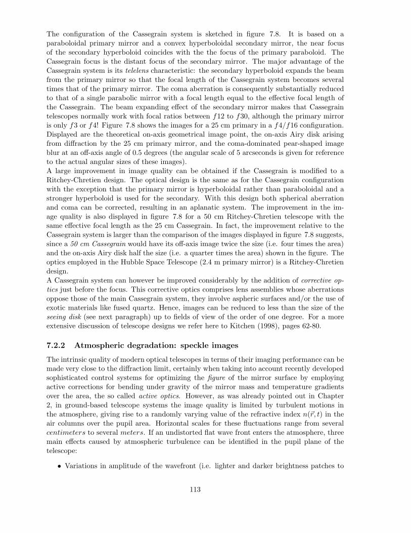
The configuration of the Cassegrain system is sketched in figure 7.8. It is based on aparaboloidal primary mirror and a convex hyperboloidal secondary mirror, the near focusof the secondary hyperboloid coincides with the the focus of the primary paraboloid. TheCassegrain focus is the distant focus of the secondary mirror. The major advantage of theCassegrain system is its telelens characteristic: the secondary hyperboloid expands the beamfrom the primary mirror so that the focal length of the Cassegrain system becomes severaltimes that of the primary mirror. The coma aberration is consequently substantially reducedto that of a single parabolic mirror with a focal length equal to the effective focal length ofthe Cassegrain. The beam expanding effect of the secondary mirror makes that Cassegraintelescopes normally work with focal ratios between f12 to f30, although the primary mirroris only f3 or f4! Figure 7.8 shows the images for a 25 cm primary in a f4/f16 configuration.Displayed are the theoretical on-axis geometrical image point, the on-axis Airy disk arisingfrom diffraction by the 25 cm primary mirror, and the coma-dominated pear-shaped imageblur at an off-axis angle of 0.5 degrees (the angular scale of 5 arcseconds is given for referenceto the actual angular sizes of these images).A large improvement in image quality can be obtained if the Cassegrain is modified to aRitchey-Chretien design. The optical design is the same as for the Cassegrain configurationwith the exception that the primary mirror is hyperboloidal rather than paraboloidal and astronger hyperboloid is used for the secondary. With this design both spherical aberrationand coma can be corrected, resulting in an aplanatic system. The improvement in the im-age quality is also displayed in figure 7.8 for a 50 cm Ritchey-Chretien telescope with thesame effective focal length as the 25 cm Cassegrain. In fact, the improvement relative to theCassegrain system is larger than the comparison of the images displayed in figure 7.8 suggests,since a 50 cm Cassegrain would have its off-axis image twice the size (i.e. four times the area)and the on-axis Airy disk half the size (i.e. a quarter times the area) shown in the figure. Theoptics employed in the Hubble Space Telescope (2.4 m primary mirror) is a Ritchey-Chretiendesign.A Cassegrain system can however be improved considerably by the addition of corrective op-tics just before the focus. This corrective optics comprises lens assemblies whose aberrationsoppose those of the main Cassegrain system, they involve aspheric surfaces and/or the use ofexotic materials like fused quartz. Hence, images can be reduced to less than the size of theseeing disk (see next paragraph) up to fields of view of the order of one degree. For a moreextensive discussion of telescope designs we refer here to Kitchen (1998), pages 62-80.

7.2.2 Atmospheric degradation: speckle images

The intrinsic quality of modern optical telescopes in terms of their imaging performance can bemade very close to the diffraction limit, certainly when taking into account recently developedsophisticated control systems for optimizing the figure of the mirror surface by employingactive corrections for bending under gravity of the mirror mass and temperature gradientsover the area, the so called active optics. However, as was already pointed out in Chapter2, in ground-based telescope systems the image quality is limited by turbulent motions inthe atmosphere, giving rise to a randomly varying value of the refractive index n(�r, t) in theair columns over the pupil area. Horizontal scales for these fluctuations range from severalcentimeters to several meters. If an undistorted flat wave front enters the atmosphere, threemain effects caused by atmospheric turbulence can be identified in the pupil plane of thetelescope:

• Variations in amplitude of the wavefront (i.e. lighter and darker brightness patches to

113

Figure 7.9: Left panel: short exposure speckle image. Right panel: long exposure showing thesmoothed ”seeing” disk of the observed point source.

the ”eye”) corresponding to concentration or spreading of the wavefront energy (scin-tillation).

• Variation in the angle of the mean tangent plane to the wavefront causing angular motionof the image. Characteristic wavefront slopes are of the order of a few μm’s/meter.

• Reduction of spatial coherence of the wavefront across the pupil plane due to randomfluctuation of the phase, that leads to smearing of the image, resulting in image sizesmuch larger than from diffraction alone.

These effects can be described by introducing a new, instantaneous, pupil function which israndom and complex:

P (�r, t) = P (�r)ψ(�r, t) (7.25)

in which P (�r) represents the simple geometrical pupil function introduced in equation ( 7.4)and ψ(�r, t) represents a wavefront that randomly varies in amplitude and phase. During avery short exposure, of the order of a few milliseconds, one may consider the wavefront frozenin its instantaneous shape. If we neglect for the moment the amplitude fluctuations (i.e.scintillation), we can write:

ψ(�r, t) = e−iφ(�r, t) (7.26)

in which the phase of the wave, φ(�r, t), is a random variable whose spatial statistical distri-bution is determined by the properties of the randomly varying value of the refractive indexin the turbulent cells of the overlaying atmosphere. If we consider an atmospheric layer ofthickness Δh that is large compared to the scale size of the turbulent cells, so that Gaussianstatistics apply (i.e. the central limit theorem), the phase shift produced by the refractiveindex fluctuations is:

φ(�r, t) = k

h+Δh∫h

n(�r, t, z)dz (7.27)

with n(�r, t, z) the refractive index random variable, z the vertical coordinate and k = 2π/λthe wave number. This randomly varying phase shift describes the effects of angular motionand smearing of the image, the amplitude variations may often be neglected if the turbulenceis not very severe.Hence we have now an instantaneous, random, pupil function:

P (�r, t) = P (�r)e−iφ(�r, t) (7.28)

114

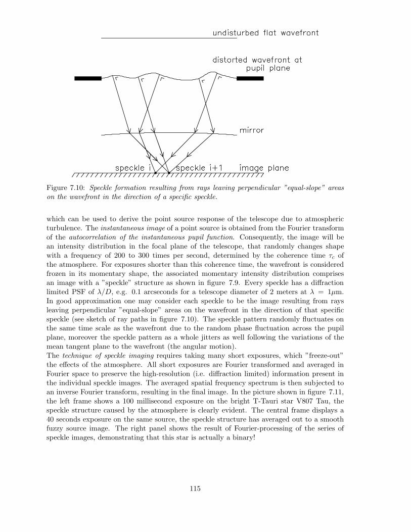
Figure 7.10: Speckle formation resulting from rays leaving perpendicular ”equal-slope” areason the wavefront in the direction of a specific speckle.

which can be used to derive the point source response of the telescope due to atmosphericturbulence. The instantaneous image of a point source is obtained from the Fourier transformof the autocorrelation of the instantaneous pupil function. Consequently, the image will bean intensity distribution in the focal plane of the telescope, that randomly changes shapewith a frequency of 200 to 300 times per second, determined by the coherence time τc ofthe atmosphere. For exposures shorter than this coherence time, the wavefront is consideredfrozen in its momentary shape, the associated momentary intensity distribution comprisesan image with a ”speckle” structure as shown in figure 7.9. Every speckle has a diffractionlimited PSF of λ/D, e.g. 0.1 arcseconds for a telescope diameter of 2 meters at λ = 1μm.In good approximation one may consider each speckle to be the image resulting from raysleaving perpendicular ”equal-slope” areas on the wavefront in the direction of that specificspeckle (see sketch of ray paths in figure 7.10). The speckle pattern randomly fluctuates onthe same time scale as the wavefront due to the random phase fluctuation across the pupilplane, moreover the speckle pattern as a whole jitters as well following the variations of themean tangent plane to the wavefront (the angular motion).The technique of speckle imaging requires taking many short exposures, which ”freeze-out”the effects of the atmosphere. All short exposures are Fourier transformed and averaged inFourier space to preserve the high-resolution (i.e. diffraction limited) information present inthe individual speckle images. The averaged spatial frequency spectrum is then subjected toan inverse Fourier transform, resulting in the final image. In the picture shown in figure 7.11,the left frame shows a 100 millisecond exposure on the bright T-Tauri star V807 Tau, thespeckle structure caused by the atmosphere is clearly evident. The central frame displays a40 seconds exposure on the same source, the speckle structure has averaged out to a smoothfuzzy source image. The right panel shows the result of Fourier-processing of the series ofspeckle images, demonstrating that this star is actually a binary!

115

Figure 7.11: Left frame: a 100 millisecond exposure on the bright T Tauri star V807 Tau,the speckle structure is clearly seen. Middle frame: a 40 second exposure on the same source,the speckles have averaged to a smooth fuzzy source. Right panel: Speckle-processed imagerevealing the binary nature of the source.

7.2.3 Seeing: the Fried parameter

As is evident from figures 7.9 and 7.11, long exposures combine speckle images into a severelybroadened image, this broadening is called seeing. The resulting smoothed PSF, the so-calledseeing disk, is slightly broader than a single speckle pattern and amounts to ≈ one arcsecond.This seeing-value of one arcsecond corresponds to the diffraction limit of a 10 cm diametertelescope at λ = 0.5μm. The merit of using larger optical telescopes is, therefore, not primarilysharper images but sensitivity owing to their much larger light collecting power!The observed intensity at each point of a long-exposure image is simply the time-averagedinstantaneous intensity I(�Ω) = E

{I(�Ω , t)

}:

I(�Ω) = E{s(�Ω) ∗ h(�Ω, t)

}= s(�Ω) ∗ E

{h(�Ω, t)

}(7.29)

with s(�Ω) the intensity of a constant quasi-monochromatic source and h(�Ω, t) the randomlyvariable PSF.The spatial frequency spectrum of the seeing disk in long exposure images follows from thecomputation of the normalised mean OTF H(�ζ ) = E

{H(�ζ , t)

}which, according to equation

( 7.14), equals the normalised mean autocorrelation of the pupil function in the case of centrallysymmetric pupils:

H(�ζ ) = E

{1∫ ∫

pupil planeP 2(�ζ ′)d�ζ ′

∫ ∫pupil plane

P (�ζ ′)e−iφ(�ζ ′, t)P (�ζ ′ − �ζ )eiφ(�ζ ′−�ζ , t)d�ζ ′}

=1∫ ∫

pupil planeP 2(�ζ ′)d�ζ ′

∫ ∫pupil plane

P (�ζ ′)P (�ζ ′ − �ζ )E{e−i[φ(�ζ ′, t)−φ(�ζ ′−�ζ , t)]

}d�ζ ′

(7.30)

with �ζ ′ ≡ �r ′/λ, �ζ ≡ �r/λ and d�ζ ′ ≡ d�r ′/λ2 the scaled pupil position vectors and differentialarea, normalised to the wavelength λ. The phase fluctuations φ(�ζ , t) over the wavefront inthe pupil plane can be regarded as resulting from a large number of perturbations in theoverlaying atmosphere, which are mutually phase independent. According to the central limittheorem the distribution of the random variable φ(�ζ , t) will be Gaussian with zero mean overboth time and space. If x is a real Gaussian random variable, it is straightforward to show(verify this yourself!) that:

E {exp(ix)} = exp[−1

2E{x2}]

(7.31)

116

and consequently we have for the expectation value in the integrand of equation ( 7.30):

E{exp[−i[φ(�ζ ′, t) − φ(�ζ ′ − �ζ , t)]

]}= exp

[−1

2E{[φ(�ζ ′, t) − φ(�ζ ′ − �ζ , t)

]2}]

= exp[−1

2Qφ(�ζ )

](7.32)

where we have introduced a structure function for the phase:

Qφ(�ζ ) = E{[φ(�ζ ′, t) − φ(�ζ ′ − �ζ , t)

]2}

= 2[E{φ2(�ζ ′, t)

}− E

{φ(�ζ ′, t)φ(�ζ ′ − �ζ , t)

}](7.33)

This structure function for the phase distribution over the wavefront can be derived fromthe structure function of the refractive index for homogeneous and isotropic turbulence. Weshall forego this calculation here and refer to the treatment by F. Roddier: The Effects ofAtmospheric Turbulence in Optical Astronomy (Progress in Optics XIX,281,1981). The phasecorrelation on the perturbed wavefront expressed by equation ( 7.33) can be characterised bya wavelength dependent correlation length rc = λζc. A detailed computation involving theafore mentioned structure function of the refractive index yields:

Qφ(�r) = 2( |�r|rc

)5/3

=⇒ Qφ(�ζ ) = 2

(λ|�ζ|rc

)5/3

(7.34)

with:

rc =

⎡⎣1.45 k2

∞∫0

C2n(z) dz

⎤⎦−3/5

(7.35)

in which the wave number k = 2π/λ and where C2n(z) represents the refractive index structure

constant, that strongly depends on the altitude z, typical values range from 10−14 m−2/3 nearthe ground decreasing to 10−17 m−2/3 at an altitude of 10 km.The common case of a circular pupil with a diameter D � rc yields for the mean value ofthe normalised OTF:

H(p) = exp −(λp

rc

)5/3

(7.36)

where we have again used the scalar spatial frequency variable p following the limitation tocircular symmetry. The point source response is the Fourier Transform of H(p).It is customary to express the degraded resolution in terms of the diameter DF of a diffractionlimited circular pupil which would give an image of the same angular extent as the seeing disk.DF is the so-called Fried parameter, which can be computed from:

∞∫0

H(p)p dp =

DF /λ∫0

2π

⎡⎣arccos( λp

DF

)−(λp

DF

)(1 −

(λp

DF

)2) 1

2

⎤⎦ p dp (7.37)

For the lefthand integral in equation (7.37):

∞∫0

p

[exp −

(λp

rc

)5/3]dp (7.38)

117

we can introduce the variable x = [(λp)/rc]5/3 and rewrite this as:

35r2cλ2

∞∫0

x1/5 e−x dx =35r2cλ2

Γ(

65

)= 0.55

r2cλ2

(7.39)

Introducing a change of variable x = (λp)/DF , we can rewrite the righthand integral ofequation ( 7.37) as:

(2π

D2F

λ2

)⎡⎣ 1∫0

(x arccos x − x2

√(1 − x2)

)dx

⎤⎦ =

(2π

D2F

λ2

)(π

16

)=

D2F

8λ2(7.40)

Hence, the Fried parameter relates to the phase correlation length rc on the perturbed wave-front as:

D2F = 4.4 r2c =⇒ DF = 2.1 rc (7.41)

and, implementing expression (7.35), we find:

DF =

⎡⎣0.423 k2

∞∫0

C2n(z) dz

⎤⎦−3/5

= 0.185λ6/5

⎡⎣ ∞∫

0

C2n(z) dz

⎤⎦−3/5

(7.42)

Subsequently, expressing the phase structure function Qφ(�r) and the mean OTF H(p) for acircular aperture in terms of the Fried parameter DF , we can rewrite equations (7.34) and(7.36) as:

Qφ(�r) = 6.88( |�r|DF

)5/3

H(p) = exp

[− 3.44

(λp

DF

)5/3]

(7.43)

From this we see that the spatial frequency cut-off p ≈ DF /λ (H(p) ≈ 0.03), consequentlythe angular resolution Δθ ≈ λ/DF . This value is often called the seeing angle or simply theseeing. A typical value for DF in the visible range of the spectrum ranges between 10 and20 cm. So if for instance the seeing at the Keck 10-m telescope is 10 cm, the image qualityis no better than that provided by a 10-cm amateur telescope. From expression (7.42) it isclear that the Fried parameter is highly chromatic: ∼ λ6/5. This means that the coherencearea rapidly increases towards the infrared: a DF of 20 cm at 0.5 μm increases to almost 1.2meters at 2.2 μm.

7.2.4 Real time correction: principle of adaptive optics

Under certain conditions, it is possible to restore spatial frequencies, filtered by the atmo-sphere, in real time. This is the aim of adaptive optics, which has developed very rapidlysince 1985.An atmospheric compensation system employing active optics contains three main compo-nents: a sampling system, a wavefront sensor and a correction system. The sampling systemprovides the sensor with the distorted wavefront, in astronomy this normally entails a partlyreflecting mirror, which typically diverts ≈ 10 percent of the radiation to the sensor, allowingthe bulk of the radiation to proceed to form the main image. Many adaptive optics systemsuse a guide star rather than the object of interest to determine the distorsions of the wave-front. Inevitably, the guide star must be very close in the sky to the object of interest, orits wavefront will have undergone a different atmospheric distorsion. The region of the sky

118

Figure 7.12: Left: the isoplanatic area. Right: The Hartman array sensor for generation ofthe error signals caused by turbulence induced ”folds” in the flat wavefronts arriving from adistant point source.

over which the images have been similarly affected by the turbulent atmosphere is called theisoplanatic area or patch. This can in practise be as small as a few arcseconds. The notionof the isoplanatic area is displayed in the left panel of figure 7.12. This small angular sizeof the isoplanatic area means that only very few objects have suitable guide stars, thereforeartificial guide stars have been produced. This is being accomplished by the production of aso-called optical echo: a laser is tuned to one of the sodium D-line frequencies and excites thefree sodium atoms in the atmosphere at a typical height of 80 - 90 km. The glowing atomsappear like a star-like point close to the object of interest. Laser-produced guide stars possesstwo inherent problems. Due to the relatively low height of the laser-produced guide star, thelight path is slightly conical and may still differ substantially from the light path traversedby the radiation from the object of interest. Secondly, the outgoing laser beam is affectedby atmospheric turbulence as well, i.e. the guide star moves with respect to the object ofinterest, again resulting in a blurred image during long exposures.A wavefront sensor detects the distorsions in the incoming wavefront provided by the beamsplitter. Figure 7.12 shows the so-called Hartmann sensor, frequently used in astronomicaladaptive optics systems. It employs a two-dimensional array of small focussing lenses, eachof which providing an image onto an array-detector. In the absence of wavefront distorsions,each image is centered on an array-element. Distorsions in the wavefront will displace theimages from the detector centres, the degree of displacement and its direction is used to gen-erate error signals which are fed to a correction mirror. Since the atmosphere changes on atimescale of the order of ten milliseconds, the sampling, sensing and correction has to occurin a millisecond or less. The simplest systems only correct for the overall tilt of the wavefront,i.e. the mean tangent plane change of the wavefront that causes angular motion of the image.This is accomplished by suitably tilting a plane or segmented mirror placed in the light beamof the telescope in the direction opposite to the angular motion. A similar technique is the

119

so-called shift and add methodology, in that case multiple short exposure images are shifteduntil their brightest points are aligned and then added together. More sophisticated tech-niques also involve fine scale displacement corrections by employing a thin mirror capable ofbeing distorted by piezo- electric or other actuators placed undernearth the deformable mirrorsurface. The error signals of the sensor elements are then used to distort the mirror in theopposite manner relative to the distorsions of the incoming wavefront. Currently operatingsystems using this approach can achieve diffraction-limited performance in the near-infraredfor telescopes of 3 to 4 meter diameter, i.e. ≈ 0.2 arcseconds at 2 μm.The efficiency of an adaptive optics system is measured by the so-called Strehl ratio, which isthe ratio of the intensity at the centre of the corrected image to that at the centre of a perfectdiffraction-limited image of the same source. Strehl ratios of 0.6 to 0.8 are currently beingachieved.

7.3 High energy imaging

7.3.1 Grazing incidence telescopes

Wavelengths shortward of ≈ 50 nanometer and longer than ≈ 0.1 nanometer, i.e. the regimeof extreme-ultraviolet (EUV) and X-radiation, are absorbed by metallic surfaces at normalincidence, the only way to reflect and focus this radiation is to employ total reflection, sincethe refractive index of metals at these wavelenghts is slightly less than one. We can write therefractive index as:

n = 1 − δ − iβ with δ, β � 1 (7.44)

δ being a measure for the reflection and β a measure for the absorption. If we only considerthe real part of n, referring to reflection, we have n = 1 − δ. Employing Snell’s law, thecritical angle for total reflection follows from:

cos θcr = 1 − δ =⇒ θcr =√

2δ (7.45)

where the cosine term can been approximated by the first terms of the Taylor series, since δ �1. Typical values for the critical angle, depending on wavelength and specific metal(coating),range from 1 to 3 degrees. These small angles imply that focussing optics for this wavelengthrange requires very high incidence angles. It is therefore commonly referred to as grazingincidence optics, the grazing angle constitutes the angle between the incoming ray and themetal reflecting surface (i.e. the complement of the angle of incidence). Figure 7.13 showsthe reflection efficiencies ε, for several grazing angles, as a function of wavelength in A-unitsfor gold as the reflection coating deposited on the mirror substrate.

Several grazing incidence telescope configurations have been devised, the most practicaluse has been a design by Wolter comprising adjacent annular sections of a paraboloidal anda hyperboloidal surface irradiated at grazing incidence. This so-called Wolter-I telescope isdisplayed in figure 7.14, the focus of the paraboloid coincides with the focus of the ”virtual”part of the hyperboloid and the telescope focus is the focal point of the actual hyperboloidalannulus. Obviously, like in the case of the Cassegrain system, the hyperboloidal surface actsas a correction element for the large coma error of a single paraboloid for off-axis radiation. Inpractise one can obtain resolutions of the order of 1-10 arcseconds over fields of view (FOVs)of several arcminutes. Another design, also due to Wolter, is shown in figure 7.15. In thiscase the grazing incidence rays reflect from the inner surface of the paraboloidal mirror and,consecutively, from the outer surface of the hyperboloid. This so-called Wolter-II configurationis occasionally used for soft X-ray and Extreme Ultraviolet imaging, the typical grazing angles

120

Figure 7.13: Reflection efficiencies of gold for several grazing angles as a function of wave-length (in A) of the incoming radiation beam. The ordinate scale for the efficiency ε rangesfrom 0.01 to 1.

are larger than in the case of the Wolter-I configuration, however the design can be much morecompact. The location of the foci of both the individual annuli and of the full telescope isindicated in figure 7.15. A drawback of grazing incidence optics is the fact that the apertureof such telescopes is only a thin ring in projection, since only the radiation incident onto theparaboloidal annulus is transmitted to the focus. In order to increase the effective area, andhence the sensitivity of the telescope system, several systems with different radii are nestedinside each other in a confocal fashion. This is schematically shown in figure 7.16.

It is important to realise that at these short wavelengths it is normally no longer thediffraction that limits the resolution of the telescope (λ/D very small), but rather the accuracyof the surface figure such as roundness and profile. Moreover, the micro-finish of the reflectingsurface (i.e. the microscopic surface roughness) plays a dominant role in the potential qualityof the image: a surface with irregularities scatters rather than reflects the incoming beam,this will show up as ”wings” in the PSF that might contain a substantial fraction of the beamenergy. Surface smoothness of the order of 0.1 nanometer has be achieved, providing veryhigh quality X-ray mirrors.Grazing incidence mirrors can be produced in a variety of ways, either by direct machiningand polishing or by a so-called replication technique. In the latter case a thin metal reflectivelayer is deposited on a highly polished (i.e. X-ray quality) mandrel of the inverse shape tothat required for the mirror. Subsequently electro-deposition of e.g. nickel onto the mandrelis applied to built up a self-supporting mirror shell. When the appropriate thickness for the

121

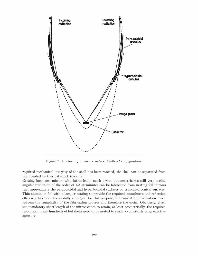
Figure 7.14: Grazing incidence optics: Wolter-I configuration.

required mechanical integrity of the shell has been reached, the shell can be separated fromthe mandrel by thermal shock (cooling).Grazing incidence mirrors with intrinsically much lower, but nevertheless still very useful,angular resolution of the order of 1-3 arcminutes can be fabricated from nesting foil mirrorsthat approximate the paraboloidal and hyperboloidal surfaces by truncated conical surfaces.Thin aluminum foil with a lacquer coating to provide the required smoothness and reflectionefficiency has been successfully employed for this purpose, the conical approximation muchreduces the complexity of the fabrication process and therefore the costs. Obviously, giventhe mandatory short length of the mirror cones to retain, at least geometrically, the requiredresolution, many hundreds of foil shells need to be nested to reach a sufficiently large effectiveaperture!

122

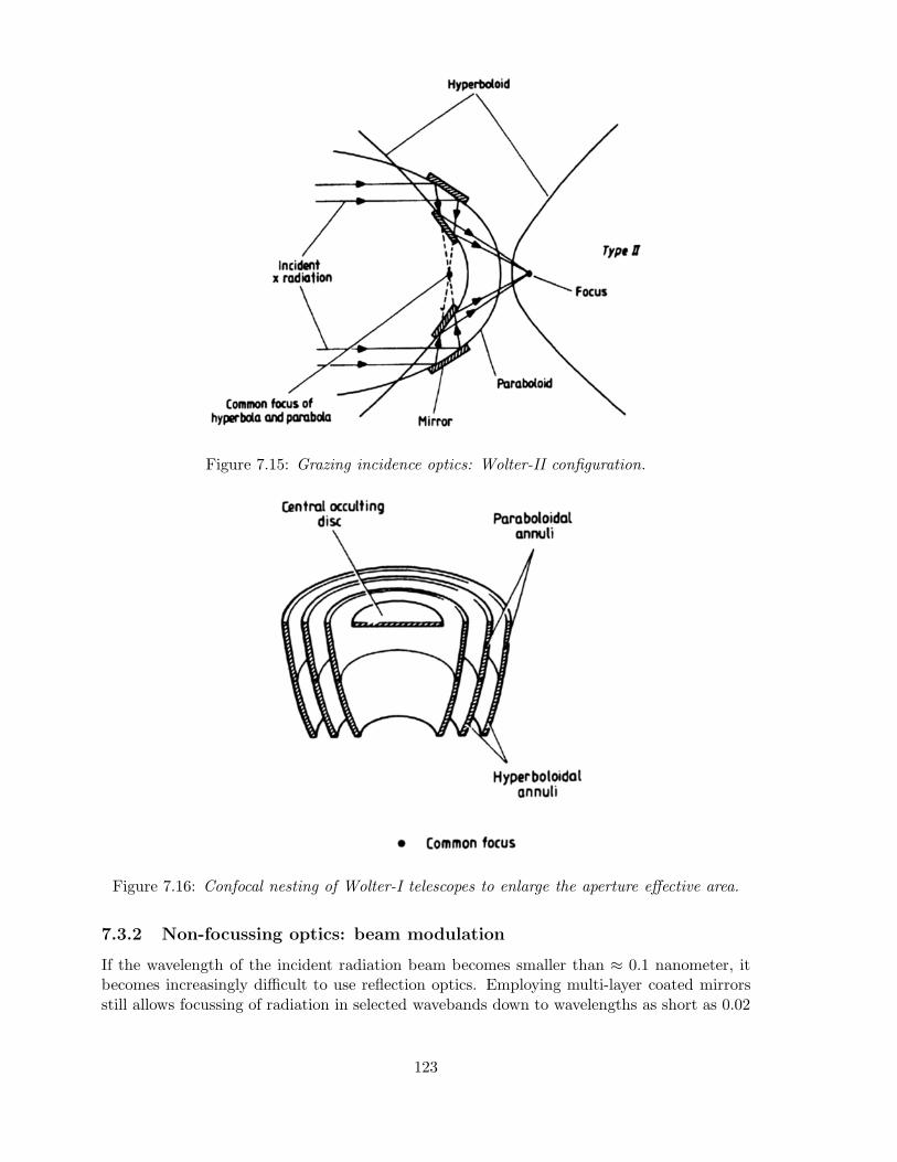
Figure 7.15: Grazing incidence optics: Wolter-II configuration.

Figure 7.16: Confocal nesting of Wolter-I telescopes to enlarge the aperture effective area.

7.3.2 Non-focussing optics: beam modulation

If the wavelength of the incident radiation beam becomes smaller than ≈ 0.1 nanometer, itbecomes increasingly difficult to use reflection optics. Employing multi-layer coated mirrorsstill allows focussing of radiation in selected wavebands down to wavelengths as short as 0.02

123

Figure 7.17: Elements of a coded mask telescope

nanometer, but not much further. Therefore, images will have to be obtained by other means.In the photon energy range where the photo-electric effect is still dominant, imaging canbe accomplished by applying the coded mask technique. In the photon energy range whereCompton scattering and pair creation are the dominant interaction processes, the kinematicsof the interaction processes can be used to extract directional information to built up images.In that case telescope and detecting device have become one. We shall treat these latter twotechniques under Gamma-ray imaging, and shall first briefly describe the principle of codedmask imaging.Coded mask imaging is based on an old principle, the Camera Obscura, where a hole in amask allows an image to form on a screen. The smaller the hole , the better the angularresolution, but unavoidably at the expense of the irradiance. Moreover, if the hole becomestoo small, diffraction effects will degrade the resolution. In the X-ray domain diffractioneffects become negligible considering the small wavelengths involved, and the irradiance levelcan be enhanced by employing a large number of holes, so that the transmission of the maskmay reach a value of ≈ 50 percent. The resulting image from such a multi-hole mask is alinear superposition of the images produced by each individual hole. The distribution of theholes needs to be done in such a way that the brightness distribution of the illuminatingcelestial source can be reconstructed in an unambiguous fashion from the measured intensitydistribution in the registered image. The appropriate pattern of holes and stops constitutesa so-called coded mask, this surface is described by a two-dimensional transmission functionM(x, y). If we assume an extended radiation source S(x, y), the intensity distribution D(x, y)on the detector can be written as a convolution:

D(x, y) = M(x, y) ∗ S(x, y) + N (7.46)

with N representing the detector noise.The working principle of the coded mask camera is displayed in figure 7.17. To reconstructthe brightness distribution of the extended celestial radiation source, the image D(x, y) needsto be deconvolved with the transmission function M(x, y) of the mask. The simplest operationto perform this deconvolution is a two-dimensional cross-correlation of the mask transmissionfunction with the detector image. Formally, an estimate of the source distribution, Σ(x, y),can be obtained by applying a decoding function A(x, y):

Σ(x, y) = A(x, y) ∗ D(x, y) = A(x, y) ∗ M(x, y) ∗ S(x, y) + A(x, y) ∗ N (7.47)

If the image detector were to be noise free, there should exist a one-to-one correspondencebetween S and Σ, hence we require A ∗ M = δ (Kronecker delta). Secondly, the noise

124

Figure 7.18: Left: A BeppoSAX WFC coded mask picture of a sky region near the GalacticCentre in terms of a raw photon intensity map. The dark bars and stripes reflect the detec-tor window support structure. Right: the deconvolved detector image showing the wealth ofcompact X-ray sources in the Galactic Bulge area.

distribution should preferably be uniform over the deconvolved image. Mask patterns M(x, y)that satisfy these two requirements are designated optimal.Note: It is important to realize that the noise level and distribution in the detector imagedepends on the brightness distribution of the sky within the field of view of the coded masktelescope. Each source in the sky field observed does not only contribute to its specific location(i.e. pixel) in the detector image but also to all the other image pixels. This means that all theradiation sources in the observed sky field contribute to the noise level of the detector image.The angular resolution of a coded mask telescope is directly related to the size me of anindividual mask element and the distance l between the mask plane and the detector plane:

δθres = arctan(me/l) (7.48)

This resolution implies a proper sampling by the image detector of the mask element me, theNyquist criterion is amply satisfied for a spatial resolution of the detector de ≈ me/3. Usuallythe size of the mask pattern covers the same area as the image detector and the sensitivityis not uniform across the whole field of view, being dependent on the coded fraction of thedetector that is illuminated by the mask pattern. Hence, the characterisation of the field ofview of a coded mask telescope can be done along three coding limits: the fully coded limit,the semi-coded limit and the zero-coded limit. If the mask has the same size as the imagedetector and does not comprise repetition of a (smaller size) basic coding pattern, the fieldthat is fully coded equals zero. The field of view at half the sensitivity will be equal to the solidangle subtended by the mask as seen from the image detector. Several coded mask telescopeshave been developed and built for hard X-ray and low-energy gamma-ray detection, e.g. theDutch-Soviet coded mask X-ray camera on the Soviet MIR Space Station, the French codedmask telescope SIGMA onboard the Soviet GRANAT spacecraft, the Dutch-Italian Wide Fieldcoded mask Cameras on the BeppoSAX satellite and the low-energy Gamma-ray Imager onthe European INTEGRAL Space Observatory. The Wide-Field coded mask Cameras (WFC)

125

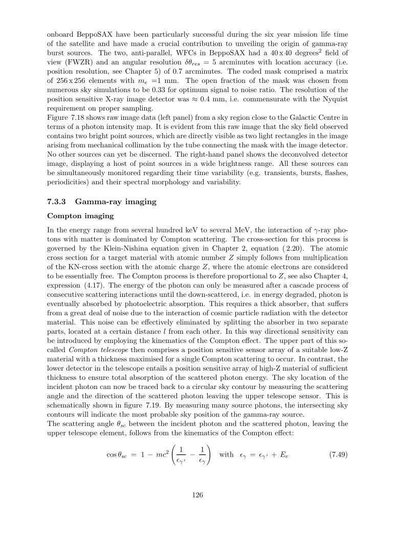
onboard BeppoSAX have been particularly successful during the six year mission life timeof the satellite and have made a crucial contribution to unveiling the origin of gamma-rayburst sources. The two, anti-parallel, WFCs in BeppoSAX had a 40 x 40 degrees2 field ofview (FWZR) and an angular resolution δθres = 5 arcminutes with location accuracy (i.e.position resolution, see Chapter 5) of 0.7 arcminutes. The coded mask comprised a matrixof 256 x 256 elements with me =1 mm. The open fraction of the mask was chosen fromnumerous sky simulations to be 0.33 for optimum signal to noise ratio. The resolution of theposition sensitive X-ray image detector was ≈ 0.4 mm, i.e. commensurate with the Nyquistrequirement on proper sampling.Figure 7.18 shows raw image data (left panel) from a sky region close to the Galactic Centre interms of a photon intensity map. It is evident from this raw image that the sky field observedcontains two bright point sources, which are directly visible as two light rectangles in the imagearising from mechanical collimation by the tube connecting the mask with the image detector.No other sources can yet be discerned. The right-hand panel shows the deconvolved detectorimage, displaying a host of point sources in a wide brightness range. All these sources canbe simultaneously monitored regarding their time variability (e.g. transients, bursts, flashes,periodicities) and their spectral morphology and variability.

7.3.3 Gamma-ray imaging

Compton imaging

In the energy range from several hundred keV to several MeV, the interaction of γ-ray pho-tons with matter is dominated by Compton scattering. The cross-section for this process isgoverned by the Klein-Nishina equation given in Chapter 2, equation ( 2.20). The atomiccross section for a target material with atomic number Z simply follows from multiplicationof the KN-cross section with the atomic charge Z, where the atomic electrons are consideredto be essentially free. The Compton process is therefore proportional to Z, see also Chapter 4,expression (4.17). The energy of the photon can only be measured after a cascade process ofconsecutive scattering interactions until the down-scattered, i.e. in energy degraded, photon iseventually absorbed by photoelectric absorption. This requires a thick absorber, that suffersfrom a great deal of noise due to the interaction of cosmic particle radiation with the detectormaterial. This noise can be effectively eliminated by splitting the absorber in two separateparts, located at a certain distance l from each other. In this way directional sensitivity canbe introduced by employing the kinematics of the Compton effect. The upper part of this so-called Compton telescope then comprises a position sensitive sensor array of a suitable low-Zmaterial with a thickness maximised for a single Compton scattering to occur. In contrast, thelower detector in the telescope entails a position sensitive array of high-Z material of sufficientthickness to ensure total absorption of the scattered photon energy. The sky location of theincident photon can now be traced back to a circular sky contour by measuring the scatteringangle and the direction of the scattered photon leaving the upper telescope sensor. This isschematically shown in figure 7.19. By measuring many source photons, the intersecting skycontours will indicate the most probable sky position of the gamma-ray source.The scattering angle θsc between the incident photon and the scattered photon, leaving theupper telescope element, follows from the kinematics of the Compton effect:

cos θsc = 1 − mc2(

1εγ ′

− 1εγ

)with εγ = εγ ′ + Ee (7.49)

126

Figure 7.19: Kinematics of the Compton effect. The sky location of the incident photon can betraced back to a circular contour by measuring the scattering angle φ = θsc and the orientationof the line element AB.

in which εγ represents the energy of the incoming photon, εγ ′ the energy of the first scat-tered photon and Ee the energy of the scattered Compton electron. The direction of the firstCompton scattered photon, the line element AB in figure 7.19, can be reconstructed frommeasuring the interaction positions in the upper and lower telescope elements respectively.Figure 7.20 depicts such a telescope configuration for the case of the Comptel instrument,launched in 1991 aboard the Compton Gamma-Ray Observatory (Compton GRO) by NASA.The energy and position of the scattered Compton electron is measured in the upper de-

tector, comprising a liquid scintillator array in which each element is viewed by a numberof photomultipliers to obtain position resolution within a single array module. The energyand position of the first scattered photon is measured in the lower detector, constitutingan array of optically thick NaI(Tl) scintillator crystals for total absorption of the scatteredgamma-ray photon, again a cluster of photomultipliers is used to determine the position ofthe absorbed scattered photon inside a single NaI-module. By requiring simultaneous triggersfrom the upper and lower detector arrays within a small time window commensurate with thetime-of-flight tTOF ≈ l/c of the first scattered photon from the upper to the lower detectorarray, almost all background events can be eliminated. This can be understood by remem-bering that these background events either trigger only one detector array or they producethe wrong time sequence (practically all background events are produced in the high-masshigh-Z absorber array). This particular Compton telescope is the most sensitive instrumentin the medium-energy gamma-ray range (0.5-30 MeV) developed and operated thus far. Theangular resolution depends on the measurement accuracy of the orientation of the line ele-ment AB and the scattering angle θsc and ranges from 1.7 to 4.4 degrees (FWHM) dependingon the gamma-ray energy. The accuracy of source position determination, i.e. the positionresolution, is 5-30 arcminutes dependent on photon energy. The field of view (FOV) of such

127

Figure 7.20: Configuration of the Compton telescope as flown on the NASA Compton Gamma-Ray Observatory (Compton-GRO). The upper detector array (the scatterer) consists of 7 cylin-drical modules filled with liquid scintillator (NE 213A, geometric area ≈ 0.42 m2), each viewedby several photomultiplier tubes to obtain position resolution. The lower detector (the absorber)consists of 14 cylindrical modules of an anorganic scintillator (NaI(Tl), geometric area ≈ 0.86m2, each of them also viewed by a multitude of photomultipliers. The distance between bothdetector assemblies is 1.5 meter.

Figure 7.21: Gamma-ray map of the Orion region in the 3-7 MeV energy range as measuredby Comptel. The orange-white contours indicate the locations of gamma-ray enhancements,the blue contours represent the locations of the densest interstellar gas clouds

128

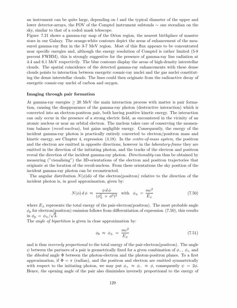
an instrument can be quite large, depending on l and the typical diameter of the upper andlower detector-arrays, the FOV of the Comptel instrument subtends ∼ one steradian on thesky, similar to that of a coded mask telescope.Figure 7.21 shows a gamma-ray map of the Orion region, the nearest birthplace of massivestars in our Galaxy. The orange-white contours depict the areas of enhancement of the mea-sured gamma-ray flux in the 3-7 MeV region. Most of this flux appears to be concentratednear specific energies and, although the energy resolution of Comptel is rather limited (5-8percent FWHM), this is strongly suggestive for the presence of gamma-ray line radiation at4.4 and 6.1 MeV respectivily. The blue contours display the areas of high-density interstellarclouds. The spatial coincidence of the detected gamma-ray enhancements with these denseclouds points to interaction between energetic cosmic-ray nuclei and the gas nuclei constitut-ing the dense interstellar clouds. The lines could then originate from the radioactive decay ofenergetic cosmic-ray nuclei of carbon and oxygen.

Imaging through pair formation

At gamma-ray energies ≥ 20 MeV the main interaction process with matter is pair forma-tion, causing the disappearance of the gamma-ray photon (destructive interaction) which isconverted into an electron-positron pair, both having positive kinetic energy. The interactioncan only occur in the presence of a strong electric field, as encountered in the vicinity of anatomic nucleus or near an orbital electron. The nucleus takes care of conserving the momen-tum balance (recoil-nucleus), but gains negligible energy. Consequently, the energy of theincident gamma-ray photon is practically entirely converted to electron/positron mass andkinetic energy, see Chapter 4, expression (4.18). In the centre-of-mass system, the positronand the electron are emitted in opposite directions, however in the laboratory-frame they areemitted in the direction of the initiating photon, and the tracks of the electron and positronreveal the direction of the incident gamma-ray photon. Directionality can thus be obtained bymeasuring (”visualising”) the 3D-orientations of the electron and positron trajectories thatoriginate at the location of the recoil-nucleus. From these orientations the sky position of theincident gamma-ray photon can be reconstructed.The angular distribution N(φ)dφ of the electron(positron) relative to the direction of the

incident photon is, in good approximation, given by:

N(φ) dφ ≈ φdφ

(φ2± + φ2)2with φ± =

mc2

E±(7.50)

where E± represents the total energy of the pair-electron(positron). The most probable angleφp for electron(positron) emission follows from differentiation of expression (7.50), this resultsin φp = φ±/

√3.

The angle of bipartition is given in close approximation by:

φb ≈ φ± =mc2

E±(7.51)

and is thus inversely proportional to the total energy of the pair-electron(positron). The angleψ between the partners of a pair is geometrically fixed for a given combination of φ−, φ+ andthe dihedral angle Φ between the photon-electron and the photon-positron planes. To a firstapproximation, if Φ = π (radian), and the positron and electron are emitted symmetricallywith respect to the initiating photon, we may put φ+ ≈ φ− ≈ φ, consequently ψ = 2φ.Hence, the opening angle of the pair also diminishes inversely proportional to the energy of

129

Figure 7.22: Principle of a pair conversion telescope. Thin metal converter plates are inter-leaved with tracking layers, comprising gas layers or thin 2D-position-sensitive semiconductordetector planes.

the initiating gamma-ray photon.The characteristic interaction length for pair formation is given by the radiation length (ex-

pressed in mass per unit area), which was introduced in Chapter 4, formula (4.21). Thisinteraction length is proportional to [Z(Z + 1)]−1, i.e. ≈ Z−2 for the higher Z-elements, fur-thermore it depends on the material properties under consideration but is independent of theenergy of the incident photon.A pair forming telescope can now be constructed by stacking several thin high-Z-metal con-verter plates at an appropriate mutual distance, each with a thickness of a fraction of aradiation length. The full stack is built up to a total thickness of a few radiation lengths,suitable high-Z converters comprise lead or tungsten plates. The gaps between the plates inthe stack, the so-called tracking layers, are either filled with gas or do contain thin, positionsensitive, semiconductor strip detectors, this is schematically shown in figure 7.22. Once thepair has formed, the electron/positron either ionizes the gas filling along their tracks or pro-duce an electric charge in the semiconductor strips at the particular spots of their passage.In the case of a gas filled chamber, the registered presence of a particle-pair triggers a highvoltage pulse that discharges along the particle tracks between the plates, delineating the ori-entation of their trajectories. Such a detector is called a spark chamber, the principle of whichwas already developed during the late 1950’s and the 1960’s for diagnostics in high-energyphysics at particle accelerators and in cosmic ray physics. This technique was also used in thefirst space-borne gamma-ray telescopes on SAS-2 (NASA) and COS-B (ESA), that resultedin the first (partial) maps of the high-energy gamma-ray sky. Although more sophisticatedread-out techniques, employing thin-wire grids for detection of the charges produced along theionisation tracks, were utilized in the second generation EGRET gamma-ray telecope on the

130

Figure 7.23: Schematic of the EGRET pair telescope aboard the Compton Gamma Ray Ob-servatory. The principal telescope elements are indicated, for explanation see text.

Compton Gamma-Ray-Observatory, the basic detection principle remained unaltered. Figure7.23 shows the main constitutive elements of this pair telescope, that was designed to coverthe energy range from 20 MeV to 30 GeV.The instrument uses a multiple-layer spark chamber with thin metal pair-conversion plates.The total energy of the gamma-ray photon is measured by a NaI(Tl) scintillation counterbeneath the spark chambers to provide good energy resolution over a wide dynamic range inenergy. The absorption proces involves a cascade of non-thermal Bremsstrahlung losses bythe pair-particles and renewed pair formation by the Bremsstrahlung photons, followed byCompton scattering and finally photo-electric absorption until all the initial photon energyhas been depleted. The instrument is covered by a plastic scintillator anticoincidence dometo discriminate against charged particle radiation incident on the telescope. Moreover, tofurther separate background events from true celestial gamma-rays, a time-of-flight system isincorporated similar to the one incorporated in the Compton telescope, to ensure that theradiation is arriving in the proper time sequence.The EGRET telescope instantaneously covers a wide field of view of ∼ 0.6 steradians, the

position resolution is dependent on photon energy and source strength. For a strong, hardspectrum, gamma-ray source this position resolution amounts to ∼ 5 - 10 arcminutes. As out-lined above, at lower photon energies the pair-angle is large, however the kinetic energy of thepair particles is relatively low and they suffer from scattering in the metal converter plates ofthe spark chamber. This introduces stochastic fluctuations in the particle-track determina-

131

Figure 7.24: The third EGRET all sky map of gamma-ray point sources above 100 MeV. Themajority of these sources remains as yet unidentified

tion due to the straggling behaviour of the electron/positron pairs. At high photon energies,the statistical fluctuations due to straggling are less severe, since the pair particles possessa much higher kinetic energy. However, as we have seen, the separation angle ψ diminisheswith 1/E±, which makes accurate determination of the bipartition angle less straightforward.Figure 7.24 shows the third catalogue of EGRET detected gamma-ray point sources above100 MeV, the large majority of these sources has not yet been identified. This is either dueto the limited positional resolution of the EGRET instrument or to an intrinsic lack of coun-terparts at other wavelengths.

The next generation gamma-ray telescope GLAST (Gamma-ray Large Area Space Tele-scope), to be launced by NASA in 2006, exploits a new technology in track detection: thegas-filling of the chamber has been replaced by solid state detectors as the tracking material.This allows for improved energy and spatial resolution. An energy resolution as good as 5percent(FWHM) is aimed for and a position resolution as good as a few arcminutes for asingle gamma-ray photon and of the order of ≤ 30 arcseconds for a strong gamma-ray source.In addition, a major advantage is the fact that a replenishable supply of chamber gas is nolonger needed, which will make a much longer mission life time potentially feasible.The baseline design for the GLAST pair forming telescope involves a modular tracker arraycomprising four-by-four tower modules (total of 16), of which each module consists of inter-leaved planes of thin lead converter sheets and silicon-strip solid state detectors. The siliconstrips are arranged in a stack of 19 pairs-of-planes, one plane of each pair for read-out in thex-direction, the other plane of the pair for read-out in the perpendicular y-direction. Whenthe electron/positron interacts with such a plane-pair, an accurate position can be determinedin two dimensions. The third dimension of the track is derived by analysing the signals fromconsecutive adjacent planes as the particle travels downward through the stack towards theenergy calorimeter. A multi-fold (at least three) coincidence between adjacent plane-pairstriggers the read-out sequence of the particle tracks. Figure 7.25 shows the concept of thetower modules and the stack of tracking detectors. The energy bandwidth of GLAST rangesfrom ∼ 15 MeV to ≥ 100 GeV, with a field of view in excess of 2 steradians. The sensitivityof GLAST for point source detection will be ∼ 50 times that of EGRET at 100 MeV, with

132

Figure 7.25: GLAST: concept of the tracker modules

an enhanced positional resolving power of 0.5 - 5 arcminutes.

133

Chapter 8

Spectroscopy in Astronomy

8.1 Spectral diagnostics in Astrophysics

8.1.1 Physical source parameters embedded in spectral information

8.1.2 Continuum and line emission

8.1.3 Characterisation of spectral lines

Absolute wavelength (frequency, energy) scale

Line broadening effects, line profiles and equivalent line width

8.2 Spectral separation principles

8.2.1 General concepts

Photometry and Spectroscopy

Spectral sensitivity, response and resolution

8.2.2 Interferometric separation techniques

Wavelength dispersive techniques

Etalons

Fourier Transform techniques

8.2.3 Non-interferometric separation techniques

Direct separation: photometric filtering

Wavelength dispersive: refraction

Energy dispersive techniques

Heterodyne spectroscopy

134

January 21, 2007 - SRON

Documents

Transcript of January 21, 2007 - SRON