Evidence for an intermediate-mass black hole from a gravitationally

lensed gamma-ray burst

James Paynter∗ Rachel Webster† Eric Thrane ‡§

March 30, 2021

If gamma-ray bursts are at cosmological distances, they must be gravitationally lensed occasion-ally [1, 2]. The detection of lensed images with millisecond-to-second time delays provides evidencefor intermediate-mass black holes, a population which has been difficult to observe. Several studieshave searched for these delays in gamma-ray burst light curves, which would indicate an interveninggravitational lens [3, 4, 5, 6]. Among the ∼ 104 gamma-ray bursts observed, there have been a hand-ful of claimed lensing detections [7], but none have been statistically robust. We present a Bayesiananalysis identifying gravitational lensing in the light curve of GRB 950830. The inferred lens massdepends on the unknown lens redshift zl, and is given by (1 + zl)Ml = 5.5+1.7

−0.9× 104 M (90% credibility),which we interpret as evidence for an intermediate-mass black hole. The most probable configuration,with a lens redshift zl ∼ 1 and a gamma-ray burst redshift zs ∼ 2, yields a present day number densityof ≈ 2.3+4.9

−1.6 × 103 Mpc−3 (90% credibility) with a dimensionless energy density ΩIMBH ≈ 4.6+9.8−3.3 × 10−4.

The false alarm probability for this detection is ∼ 0.6% with trial factors. While it is possible thatGRB 950830 was lensed by a globular cluster, it is unlikely since we infer a cosmic density inconsistentwith predictions for globular clusters ΩGC ≈ 8× 10−6 at 99.8% credibility. If a significant intermediate-mass black hole population exists, it could provide the seeds for the growth of supermassive black holesin the early Universe.

The evidence for a cosmological population of intermediate-mass black holes (IMBHs) is mounting. They have longbeen posited to reside in the cores of globular clusters. Dynamical friction in stellar clusters causes the most massivestars to sink to the bottom of the cluster’s gravitational potential. Since 2004, simulations have indicated that, forsmall compact clusters, stellar mergers happens within the lifetime of giant stars [8]. Critically, these mergers occurbefore the stars go supernova and disturb the system, leading to a runaway collision and the formation of a ∼ 103 Mmegastar. These short-lived monsters could seed IMBHs, which subsequently grow through accretion and mergers.Yet direct observational signatures of their existence are elusive.

Their large mass puts the majority of IMBH mergers outside the sensitivity range of the current generation ofgravitational-wave detectors. The Advanced Laser Interferometer Gravitational-wave Observatory (LIGO) [9] andVirgo [10] are sensitive to mergers with a total merger-product mass of . 400 M. Furthermore, IMBHs are too smallto be observed using the same techniques employed to detect supermassive black holes in galactic nuclei. They areeither not massive enough, or live in a state of starvation, unable to accrete enough gas to power quasar-like emission.

Astronomers are converging on the population of IMBHs from both ends of the black hole mass spectrum. Com-pact object mergers detected by LIGO-Virgo are uncovering a population of black holes edging closer to the rangetraditionally reserved for IMBHs [11], including the recent discovery of a 150 M merger product [12]. From the otherend, the lower limit on supermassive black holes in the nuclei of dwarf galaxies is descending [13]. There have beenrecent findings of compact objects with mass 104 − 105 M residing in galactic cores [14, 15]. Observations of a tidaldisruption event from the evisceration of a star by a black hole’s tidal field suggest an IMBH resides in a star clusteron the outskirts of a barred lenticular galaxy [16]. In this Letter, we provide evidence for an IMBH using gravitationallensing. Gravitational lensing is one of the few ways to directly constrain IMBH population statistics by providing anestimate for the number density of IMBHs.

In strong gravitational lensing, photon paths from a background source are distorted due to curved spacetime,producing multiple images. The relative fluxes and the difference between arrival times for each image can be used toinfer the gravitational structure of the lens. In the case of a compact lens, the mass can be directly determined upto a redshift factor. The fraction of distant sources which experience multiple-imaging is directly proportional to thedimensionless energy density of compact lenses, Ωlens ≡ ρlens/ρc [17] where ρlens is the energy density of lenses while ρcis the critical energy density required for a flat Universe. This fraction is independent of the lens mass, mlens. Stronglensing is accompanied by an overall magnification, typically a factor of a few in flux. This allows us to probe moredistant sources, or sources which would otherwise be too faint to detect.

Gamma-ray bursts (GRBs) are extremely luminous bursts of γ-rays, with peak energies of 100−300 keV. They arethought to be generated by the rapid infall of material onto a nascent stellar mass black hole, formed through eithera collapsar supernova or a compact object merger. Some of the accreting material is launched in ultra-relativistic,bipolar jets along the rotation axis. A fraction of this outflow is converted into electromagnetic radiation, which isLorentz-boosted into γ-rays. The cosmological nature of GRBs is well established by both the isotropy of observedevents [18] and redshift measurements of their optical afterglow [19]. A cosmological origin implies that at least somefraction of the GRB population must be strongly lensed [1].

Gamma-ray detectors, unlike those used for optical or infrared astronomy, have comparatively poor angular reso-lution, but good temporal resolution. Thus, we do not expect to resolve a gravitationally lensed image pair in γ-rays.However, a time delay between the two images, resulting from the differences in geometric path and relative differ-ences in gravitational field strength, can be observed. The photons which travel a longer distance arrive first, as theshorter path traverses deeper into the gravitational potential well of the lens where time dilation is stronger. Thegravitationally retarded image is dimmer than the first image. The observational signature of such an event is thusan initial γ-ray pulse followed by a duplicate “echo.” The duration of the time delay between the burst and the echo

∗jpaynter@student.unimelb.edu.au, School of Physics, University of Melbourne, Parkville, Victoria, 3010, Australia†School of Physics, University of Melbourne, Parkville, Victoria, 3010, Australia‡School of Physics and Astronomy, Monash University, Clayton, VIC 3800, Australia§OzGrav: The ARC Centre of Excellence for Gravitational Wave Discovery, Australia

1

arX

iv:2

103.

1541

4v1

[as

tro-

ph.H

E]

29

Mar

202

1

is predominantly determined by the mass of the gravitational lens, but also by the alignment of the γ-ray source withrespect to the observer-lens line-of-sight. For a point-mass lens [20, 21, 22],

(1 + zl)M =c3∆t

2G

(r − 1√r

+ ln r

)−1

. (1)

Here, ∆t is the time delay, r is the ratio of the fluxes, and (1 + zl)M is the redshifted lens mass. By measuring ∆tand r we can infer the redshifted mass (1 + zl)M .

The total number of observed GRBs is of order 104. We analyse the BATSE dataset as it is the largest availablesingle dataset at ∼ 2, 700 bursts. We include both long and short GRBs in our study. For a burst and echo tooccur within the same BATSE light curve, we require a time delay of . 240 s. The minimum detectable time delay isdetermined by the width of the γ-ray pulse; if the delay time is too short, the two images merge into one. For longGRBs, the minimum detectable time delay is ≈ 1 s, and for short bursts, it is ≈ 40 ms. This range of time delayscorresponds to a lens mass range of approximately 102 − 107 M [23, 21].

We identify preliminary lensing candidates with an auto-correlation analysis [24, 7]. We utilise the four availablebroadband energy channels of BATSE burst data independently. The equivalence principle dictates that all wavelengthsof light are equally affected by gravitational fields. This implies two constraints: the time delay is independent of thephoton energy, and the gravitational magnification of each image is identical for every wavelength. Once we haveidentified candidates, we employ Bayesian model selection to determine the Bayesian odds comparing the lensinghypothesis to the no-lensing hypothesis. Our unified framework simultaneously provides the detection significancewhile estimating the lensing parameters, which we use to infer the lens mass. To model GRB pulses, we employ thefast-rise exponential-decay (FRED) model [25]. Details are provided in the supplementary material.

We uncover one statistically significant gravitational lensing candidate: GRB 950830 (BATSE trigger 3770)—ashort γ-ray burst. The light curve for this burst is shown in Fig. 1 with the reconstructed curve of the best-fit modelplotted in black. The black curve is created by taking the mean of the curves drawn by each of the & 60, 000 posteriorsample sets at each time bin. We find that each individual pulse is best fit by a variation of the FRED pulse modelplus a sine-Gaussian function. We analyse the four available energy channels independently and find that the lensinghypothesis is preferred in each channel with ln Bayes Factors (ln(BF)) between 0.5− 7. Adding the ln(BF)s from eachof the channels, we find the total ln(BF) = 12.9 (log10 BF = 5.6) in favour of lensing, indicating strong statisticalsupport for the lensing hypothesis. A ln(BF) of eight is considered “strong evidence” in support of one model over theother [26]. Detailed fits are shown in Extended Data Figs.1-6, including an example of a ’double’ burst which is not alens (Extended Data Figs. 7-8).

Assuming a point-mass deflector, the marginalised posterior distributions for time delay and magnification ratio ofthis lensing event in Fig.2 can be used in conjunction with equation (1) to infer a redshifted lens mass of (Fig.3)

(1 + zl)Ml ∼ 5.5+1.7−0.9 × 104 M. (2)

There are three astrophysical objects in this mass range, which might serve as a lens: globular clusters, dark matterhalos, and black holes. A gravitational lens is well approximated as a point mass if most of its mass is contained withinthe region bound by the two lensed images where they bisect the cosmological plane of the lens. Taking instead anisothermal mass distribution as the gravitational lens, and integrating over all zl, zs, we find a lens velocity dispersionof ∼ 4 km s−1. From simulations, this dispersion is associated with an Navarro–Frenk–White (NFW) profile of mass∼ 105 M [27]. Globular clusters follow a similar mass–velocity dispersion scaling [28]. In either framework then,either a singular point mass, or a self-gravitating isothermal sphere, we have a consistent measurement for the mass.

Dark matter halos are numerous, and their number density can be calculated using the Press-Schechter formalism.However, each has a negligible contribution to lensing cross-section, as NFW mass distributions typically have cores,which are not sufficiently massive to produce multiple images. Globular clusters are compact enough to producemultiple images, but there are not many of them. Assuming that the Milky Way’s ∼ 200 globular clusters are typical,and that the Milky Way formed from an overdensity of approximately 20 Mpc3, then the number density of globularclusters is approximately 10 Mpc−3, giving Ωgc(105 M) ∼ 8×10−6—significantly lower than the mean density impliedby GRB 950830.

Following [17], we use the optical depth to estimate the cosmological density, Ω ∼ τ (〈zs〉). Assuming that BATSEγ-ray bursts have a mean redshift of two, the IMBH energy density is

Ωimbh

(M ∼ 104−5 M, 〈zs〉 ∼ 2

)≈ 4.6+9.8

−3.3 × 10−4. (3)

The present day number density of IMBHs is

nimbh(M ∼ 104−5 M

)≈ 2.3+4.9

−1.6 × 103 Mpc−3, (4)

(90% credibility), where we have assumed a lens redshift of zl ∼ 1. The uncertainty is from Poisson counting statistics.Thus, there should be approximately ≈ 4.6+9.8

−3.2×104 in the neighbourhood of the Milky Way. There are approximately108 stellar-mass black holes in the Milky Way [29]. Assuming all stellar mass black holes are bound to galaxies, andwith ngal ∼ 0.04 Mpc−3, then the number density of stellar mass black holes is nstellar ∼ 107 Mpc−3. Our result for theIMBH density is consistent with the stellar mass black hole density assuming that number density scales as ∼ M−1.Note that the mean redshift of Swift short GRBs is 〈zs〉 ≈ 0.8. If the GRBs in the BATSE sample had the same mean,then the inferred cosmological density Ωimbh would increase by about an order of magnitude. Extended Data Figs.9-10 give results at different source and lens redshifts.

Our estimate for Ωimbh is consistent with the null result of other GRB lens searches [6, 30], which are sensitive todifferent lens masses. The Fermi and Konus-Wind catalogues are similar in size to the BATSE GRB catalogue, andthere is ∼ 50% probability that these contain another GRB which is gravitationally lensed by an IMBH. In addition,due to the relatively flat GRB luminosity function [23], the uncertainty in nimbh derived from a single lensing event ismore significant than the potential magnification bias.

If this detection represents the first determination of the space density of IMBHs, then it may shed light on openquestions in astrophysics. How are the supermassive black holes that power quasars so massive at high redshift? AreIMBHs gravitationally bound to galaxies? Do they have observational signatures in electromagnetic or gravitationalradiation? What is their relationship to the globular cluster population? Are they the remnants of direct collapse of104−6 M dark matter or baryonic clouds in the early Universe? The identification of additional lensing candidatesin the GRB catalogues will confirm this result, and allow a more precise determination of Ωimbh.

2

References

[1] B. Paczynski. Gamma-ray bursters at cosmological distances. Astrophys. J. Lett., 308:L43–L46, 1986.

[2] B. Paczynski. Gravitational microlensing and gamma-ray bursts. Astrophys. J. Lett., 317:L51–L55, 1987.

[3] Joachim Wambsganss. A Method to Distinguish Two Gamma-Ray Bursts with Similar Time Profiles. Astrophys.J., 406:29–35, 1993.

[4] Michael A. Nowak and Scott A. Grossman. Can We Identify Lensed Gamma-Ray Bursts? Astrophys. J., 435:557–572, 1994.

[5] Julian B. Munoz, Ely D. Kovetz, Liang Dai, and Marc Kamionkowski. Lensing of Fast Radio Bursts as a Probeof Compact Dark Matter. Phys. Rev. Lett., 117(9):091301, 2016.

[6] Lingyuan Ji, Ely D. Kovetz, and Marc Kamionkowski. Strong lensing of gamma ray bursts as a probe of compactdark matter. Phys. Rev. D, 98:123523, 2018.

[7] Y. Hirose, M. Umemura, A. Yonehara, and J. Sato. Imprint of Gravitational Lensing by Population III Stars inGamma-Ray Burst Light Curves. Astrophys. J., 650:252–260, 2006.

[8] Simon F. Portegies Zwart, Holger Baumgardt, Piet Hut, Junichiro Makino, and Stephen L. W. McMillan. Forma-tion of massive black holes through runaway collisions in dense young star clusters. Nature, 428(6984):724–726,2004.

[9] J Aasi et al. Advanced LIGO. Class. Quantum Grav., 32:074001, 2015.

[10] F. Acernese et al. Advanced Virgo: a 2nd generation interferometric gravitational wave detector. Class. QuantumGrav., 32:024001, 2015.

[11] B. P. et al. Abbott. Binary Black Hole Population Properties Inferred from the First and Second Observing Runsof Advanced LIGO and Advanced Virgo. Astrophys. J., 882(2):L24, 2019.

[12] B. P. et al. Abbott. Gw190521: A binary black hole merger with a total mass of 150 M⊙. Phys. Rev. Lett.,125:101102, 2020.

[13] Andrew King. GSN 069 - A tidal disruption near miss. Mon. Not. R. Ast. Soc., 493(1):L120–L123, 2020.

[14] Tomoharu Oka, Shiho Tsujimoto, Yuhei Iwata, Mariko Nomura, and Shunya Takekawa. Millimetre-wave emissionfrom an intermediate-mass black hole candidate in the Milky Way. Nature Astronomy, 1:709–712, 2017.

[15] Shunya Takekawa, Tomoharu Oka, Yuhei Iwata, Shiho Tsujimoto, and Mariko Nomura. The fifth candidate foran intermediate-mass black hole in the galactic center. The Astrophysical Journal, 890(2):167, 2020.

[16] Dacheng Lin, Jay Strader, Eleazar R. Carrasco, Dany Page, Aaron J. Romanowsky, Jeroen Homan, Jimmy A.Irwin, Ronald A. Remillard, Olivier Godet, Natalie A. Webb, Holger Baumgardt, Rudy Wijnands, Didier Barret,Pierre-Alain Duc, Jean P. Brodie, and Stephen D. J. Gwyn. A luminous X-ray outburst from an intermediate-massblack hole in an off-centre star cluster. Nature Astronomy, 2:656–661, 2018.

[17] W. H. Press and J. E. Gunn. Method for Detecting a Cosmological Density of Condensed Objects. Astrophys.J., 185:397–412, 1973.

[18] G. J. Fishman, C. A. Meegan, R. B. Wilson, W. S. Paciesas, and G. N. Pendleton. The BATSE experiment onthe Compton Gamma Ray Observatory: status and some early results. In NASA Conference Publication, volume3137 of NASA Conference Publication, pages 26–34, 1992.

[19] E. Costa, F. Frontera, J. Heise, M. Feroci, J. in’t Zand, F. Fiore, M. N. Cinti, D. Dal Fiume, L. Nicastro,M. Orlandini, E. Palazzi, M. Rapisarda, G. Zavattini, R. Jager, A. Parmar, A. Owens, S. Molendi, G. Cusumano,M. C. Maccarone, S. Giarrusso, A. Coletta, L. A. Antonelli, P. Giommi, J. M. Muller, L. Piro, and R. C. Butler.Discovery of an X-ray afterglow associated with the γ-ray burst of 28 February 1997. Nature, 387(6635):783–785,1997.

[20] Ramesh Narayan and Sylvanie Wallington. Determination of Lens Parameters from Gravitationally LensedGamma-Ray Bursts. Astrophys. J., 399:368–372, 1992.

[21] S. Mao. Gravitational lensing, time delay, and gamma-ray bursts. Astrophys. J. Lett., 389:L41–L44, 1992.

[22] L. M. Krauss and T. A. Small. A new approach to gravitational microlensing - Time delays and the galactic massdistribution. Astrophys. J., 378:22–29, 1991.

[23] O. M. Blaes and R. L. Webster. Using Gamma-Ray Bursts to Detect a Cosmological Density of Compact Objects.Astrophys. J. Lett., 391:L63–L66, 1992.

[24] B. Geiger and P. Schneider. The light-curve reconstruction method for measuring the time delay of gravitationallens systems. Mon. Not. R. Ast. Soc., 282:530–546, 1996.

[25] J. P. Norris, R. J. Nemiroff, J. T. Bonnell, J. D. Scargle, C. Kouveliotou, W. S. Paciesas, C. A. Meegan, and G. J.Fishman. Attributes of Pulses in Long Bright Gamma-Ray Bursts. Astrophys. J., 459:393–412, 1996.

[26] E. Thrane and C. Talbot. An introduction to Bayesian inference in gravitational-wave astronomy: parameterestimation, model selection, and hierarchical models. Pub. Astron. Soc. Aust., 36:E010, 2019.

[27] Stuart Wyithe. private communication, 2020.

[28] H. Baumgardt and M. Hilker. A catalogue of masses, structural parameters, and velocity dispersion profiles of112 Milky Way globular clusters. Mon. Not. R. Ast. Soc., 478(2):1520–1557, 2018.

3

[29] Oliver D. Elbert, James S. Bullock, and Manoj Kaplinghat. Counting black holes: The cosmic stellar remnantpopulation and implications for LIGO. Mon. Not. R. Ast. Soc., 473(1):1186–1194, 2018.

[30] K. Hurley, A. E. Tsvetkova, D. S. Svinkin, R. L. Aptekar, D. D. Frederiks, S. V. Golenetskii, A. A. Kokomov,A. V. Kozlova, A. L. Lysenko, M. V. Ulanov, T. L. Cline, I. G. Mitrofanov, D. Golovin, M. L. Litvak, A. B.Sanin, W. Boynton, K. Harshman, C. Fellows, R. Starr, A. Rau, A. von Kienlin, and X. Zhang. A Searchfor Gravitationally Lensed Gamma-Ray Bursts in the Data of the Interplanetary Network and Konus-Wind.Astrophys. J., 871(1):121, 2019.

Acknowledgements

ET is supported through Australian Research Council Grant No. CE170100004 and No. FT150100281. The analysissoftware was run on The University of Melbourne’s Spartan HPC system. This research has made use of data providedby the High Energy Astrophysics Science Archive Research Center (HEASARC), which is a service of the AstrophysicsScience Division at NASA/GSFC and the High Energy Astrophysics Division of the Smithsonian Astrophysical Obser-vatory. J.P. would like to acknowledge Stuart Wyithe, Michele Trenti, and Andrew Melatos for constructive commentsin analysing and interpreting the data and results. J.P. would also like to thank Chris Shrader for assistance in un-derstanding the BATSE instrumentation, and J. Michael Burgess for constructive feedback on PyGRB and the properanalysis of γ-ray data.

Author Contributions

R.W. contributed to the initial planning of the project with later additions from J.P. and E.T. J.P. contributed thedata analysis through the pulse-fitting software package PyGRB under the guidance of E.T. The manuscript was draftedby J.P. and E.T. J.P. and R.W. contributed the gravitational lensing calculations while E.T. contributed the Bayesianframework. J.P. and E.T. responded to questions and comments from the referees. All authors discussed the resultsand commented on the manuscript.

Additional Information

Correspondence and requests for materials should be addressed to J.P.

Competing Interests

The authors declare no competing financial interests.

Methods

In this appendix we provide additional background on our methods. We start with a general overview of GRB lensingto place our research within the context of the wider field. From there, we describe our selection method for findinggravitationally lensed GRB candidates. We then discuss the statistics of photon counting in γ-ray astronomy. Weconstruct a Bayesian framework with a model for the lensing signal and γ-ray background. We go on to discuss thevalidity and robustness of our results. We include calculations to determine the optical depth to lensing for a sourcepopulation at mean redshift 〈zs〉, and provide evidence against the alternative hypothesis, that GRB 950830 was lensedby a globular cluster. We derive the uncertainty on our estimate for the number density of IMBH nimbh. We alsoinclude an estimate of the false alarm probability, both with and without trial factors. Finally, we include a candidateidentified by the autocorrelation detection algorithm but strongly rejected by our Bayesian analysis for illustrativepurposes.

A brief literature review. Gravitational lensing studies of γ-ray bursts typically come in one of two flavours.There are autocorrelation studies, which search for echoes of the γ-ray burst within the same light curve. Then thereare cross-correlation studies, which compare the light curve similarity of two separate GRB triggers on a per-bin basis.These are typically accompanied by positional coincidence statistics, which check if the GRBs have consistent sourcelocations. Our study is of the first flavour.

Traditional strong gravitational lensing refers to the multiple imaging of, e.g., quasars due to galactic-mass gravita-tional lenses. Also known as macrolensing, fiducial image separations are on the order of arcseconds, with inter-imagetime delays of days to years depending on the lens geometry and source-lens alignment. Millilensing (or mesolensing)is loosely defined as gravitational lensing due to million solar mass objects [31], and produces time delays of orderseconds. The conversion between mass and time delay is

∆t ≈ 50(Ml/106M

)seconds (5)

for a Schwarzschild potential [21]. In essence, millilensing fills the mass range between traditional strong lensing andmicrolensing whereby stars acting either alone or in unison in galaxies [32, 33, 34] produce multiple images with ∼microsecond time delays. At the more extreme end, nanolensing [35] (∼ 10−6−10−1 M), picolensing (∼ 10−12−10−7

M), and femtolensing [36] (∼ 10−16 − 10−13 M) describe deflections and interference effects due to planetary andsub-planetary mass gravitational lenses.

Autocorrelation probes millilensing echoes from ∼ 102 − 106 M gravitational lenses. The minimum lens massis determined by the temporal resolution of the instrument in addition to the variability timescale and durationof the burst. The upper mass limit is determined by the instrumental cut-off of data recording after the eventtrigger. Numerous autocorrelation searches of the BATSE database have been done using the summed 64 ms lightcurves [37, 38],[7]. Autocorrelation has been used on the Fermi GBM and Swift BAT catalogues [6], with a null resultfor lenses masses of 101 − 103 M.

4

Cross correlation studies probe time delays equal to the difference in arrival time of the two bursts. The observationof the second image is inhibited by Earth occultation. This sets a minimum observable time delay, since γ-rayobservatories typically have ∼ 90 min orbital periods. Recent work on the Fermi GBM response shows how theobservation conditions of a γ-ray burst significantly affect the inferred spectrum [39]. The effects of detector angularresponse, energy response, atmospheric scattering, accumulated particle precipitation, cosmic background and Galacticsources such as the Sun or Crab Pulsar complicate cross-correlation studies. No lensing studies have looked for GRBlensing across multiple observatories due to the inherent difficulties comparing light curves from instruments withdifferent energy responses. Cross-correlation studies of the BATSE database are also numerous [40, 41], in addition toFermi GBM [42]. A study of Konus-Wind GRBs searching for time delays of ∼ hours to ∼ 25 years (lens masses of108− 1013 M) was further augmented by the inclusion of spectral analysis [30]. Another lens identification techniqueinvolves correlation of the cumulative light curve in three spectral dimensions [43]. Correlation-free approaches include amodel-agnostic statistical method, which does take into account Poisson statistics [3], and Fourier analysis methods [4].For a comprehensive review of the gravitational lensing of transient events, see [44][30].

Candidate selection. The BATSE catalogue contains 2,704 triggered γ-ray bursts. Of these, 2,629 have discsc

bfits (64 ms) light curves available for download. Furthermore, higher-time-resolution observations are availablefor 2,446 of these γ-ray bursts, with 2,435 existing as pre-binned tte bfits (5 ms) light curves. We carry out apreliminary auto-correlation search (described below) on both the discsc bfits and tte bfits pre-binned lightcurves. Candidate detections are followed up with further analysis. In total we carry out auto-correlation on 2,679unique γ-ray bursts.

Signal (auto)-correlation can be used to measure the time delay of temporally overlapping signals of a gravitationallylensed system [24]. We define the autocorrelation function (ACF) as

C(δt) =

∑nj=0 I(tj + δt)I(tj)∑N

k=0 I(tk)2, (6)

where the sum in the numerator is taken over the bins where the two signals overlap, and the sum in the denominatoris taken over the entire input signal [24, 7]. Here, I(tj) is the count rate at time bin tj , N is the total number of bins,and n the total number of overlapping bin, where j, k index these bins in the summations.

We fit a 3rd order Savitzky-Golay filter F (δt) to the ACF. The dispersion σ between the ACF and the fit F (δt) is

σ2 =1

N

N∑j=0

[C(δtj)− F (δtj)]2, (7)

where N is the total number of bins. We identify 3σ outliers as gravitational-lensing candidates [7, 6]. Furthermore,we autocorrelate each of the four BATSE LAD energy channels, and perform the same filtering process. Gravitationallensing is achromatic for point sources, so we expect that each channel of a candidate lens GRB should autocorrelatewith the same time delay. We check that candidates yield lensing signals in both the summed light curve and individualenergy channels.

Photon counting. Photon counting is a Poisson process. High-energy satellites like BATSE accumulate photons ata series of discrete times, t1, t2, ...tn. For BATSE, these photons are collected with a sampling frequency of 500 kHz. Inmost cases, hardware limitations require that the BATSE photon arrival times (time-tagged events; TTE) are down-sampled before transmission to Earth. Only the shortest, moderately bright bursts are completely contained withinthe TTE photon-list data. Fortunately, this is the case for GRB 950830. For bursts not completely encoded in a TTElist, the counts are averaged into 64 ms bins before transmission, typically recorded for ∼ 240 s after triggering. Weignore the fact that BATSE has a small dead time (of about one clock cycle) after each count as this is only becomesimport for very bright bursts which saturate the detector.

If we consider a single time stamp ti, the likelihood of observing Ni photons is given by Poisson counting statistics

L(Ni|θ) =λNiθ,ie

−λθ,i

Ni!. (8)

The expected number of photons, λθ is

λθ,i = δtiR(tiθ). (9)

Here δti is the sampling time and R(ti|θ) is the photon rate (in units of photons per unit time) evaluated at time tiand given model parameters θ. The sampling time, δti, is subscripted with index i to account for the cases where thetime resolution in the available data changes during an event. The rate can be written as a sum of signal S (from theGRB) and background B

R(ti|θ) = B + S(ti|θ). (10)

To first order, the background is constant, but the signal varies with time according to model parameters θ.The likelihood of observing ~N = N1, N2, ... photons at times t1, t2, .... is given simply by taking the product of the

likelihood functions evaluated at different times

L( ~N |θ) =∏i

L(Ni|θ). (11)

It is easier, though, to work with the ln likelihood, which is

lnL( ~N |θ) =∑i

lnL(Ni|θ) (12)

=∑i

Ni ln(δtiB + δtiS(ti|θ)

)−(δtiB + δtiS(ti|θ)

)− log(Ni!). (13)

5

Bayesian Inference. There are two goals of Bayesian inference. The first is to derive posterior distributions p(θ|d)for our model parameters, which enables us to determine their credible intervals. The second goal is to calculate theBayesian evidence Z for a set of models in order to do model selection. Bayes theorem,

p(θ|d) =L(d|θ)π(θ)

Z, (14)

relates the posterior probability density p(θ|d) of model parameters θ given the observed data d, to a likelihood functionL(d|θ) and prior probability density π(θ). The likelihood function is a mathematical description of the probabilityof observing the data with the given model parameters. The priors are probability distributions for what we expectthese parameters to be, which, in our case, are informed by the BATSE GRB population. The evidence, also calledthe marginal likelihood, is a normalisation factor which gives information about the quality of the fit of the model tothe data averaged over parameter space, viz.

Z =

∫L(d|θ)π(θ)dθ. (15)

We define different models for

S(ti|θ,M), (16)

which we use to do Bayesian inference. The null model M = Mnull states that there is no lensing. The lens modelM = Mlens states that there is lensing. We adopt the Fast-Rise Exponential-Decay (FRED) pulse model, which isubiquitous in GRB pulse-modelling:

S(t|A, τ, ξ,∆) = A exp

[−ξ(t−∆

τ+

τ

t−∆

)]. (17)

Here, A is a vertical y-scale factor, τ is a duration scaling parameter, and ξ is an asymmetry parameter, which canbe used to adjust the skewness of the pulse. A more generalised form of this model has additional exponents, γ, ν,allowing for flatter/sharper peaks, viz.

S(t|A, τ, ξ,∆, γ, ν) = A exp

[−ξγ

(t−∆

τ

)γ− ξν

(τ

t−∆

)ν]. (18)

We call this the extended FRED model, or FRED-X for short. An analytic normalisation exists for both the FREDand FRED-X models, which decouples the maximum height of the pulses from every parameter except A, such thatA is the maximum amplitude of the pulse. Structured pulses can be modelled as either multiple overlapping pulses,or by accounting for the residual structure with another parameterisation. Thus, a single channel FRED light curverequires 4n+1 parameters, where the +1 corresponds to the constant background parameter B. For bursts with manypulses, our model is:

Stot =∑j

S(t|∆j , Aj , τj , ξj). (19)

Our prior enforces

∆j+1 > ∆j . (20)

to ensure that we are not fitting the same pulse configuration in different permutations.The FRED model has proved a popular phenomenological fit due to its simplicity and a posteriori applicability to

certain GRB progenitor models. Some authors have noted (and we confirm here) that there is a systematic residualstructure, visible after subtracting the best-fit FRED and FRED-X models from a GRB light curve, indicating animperfect fit [45]. We model these residuals using a sine-Gaussian wave packet

res(t) = Ares exp

[−(t−∆res

τres

)2]

cos (ωt+ ϕ) , (21)

as it is ubiquitous in physics and provides an adequate fit to the residual structure. The residual is part of our signalmodel, so we fit it simultaneously to any FRED pulses:

S(t|θ) = S(t|θfred) + res(t|θres). (22)

The lens model is similar to the null model, but with two extra parameters used to describe the delayed signal:

Slens(θlens) = S(t|θnull) + r−1 · S(t+ ∆t|θnull) (23)

where the lens parameter vector θlens subsumes the null parameter vector θnull in addition to the time delay, ∆t, andmagnification ratio, r. The parameter r reduces the amplitude of the delayed signal while the parameter ∆t describesthe size of the delay. Thus, the lens model requires 4n+ 3 parameters, where nlens is typically about half nnull.

In order to determine which model is favoured, we calculate the Bayesian evidence for each model:

Znull =

∫dθnull Lnull( ~N, θnull)π(θnull), (24)

Zlens =

∫dθlens Llens( ~N, θlens)π(θlens). (25)

Here π denotes a prior distribution and ~N is the vector of photon counts. Once we have each evidence, we obtain theln Bayes factor

ln(BF) = lnZnull − lnZlens. (26)

The Bayes factor is a statistically rigorous measure of which model the data prefer. A ln Bayes factor of eight,ln(BF) & 8, is considered “strong evidence” in support of one model over the other [26].

To perform parameter estimation and evidence calculations we use the Bilby Bayesian inference library [46]. Weemploy nested sampling [47, 48], taking advantage of the multi-ellipsoid bounding method [49], with dynamicallyupdated sampling points [50]. Results tend to be unimodal, but we use multi-ellipsoid bounding regardless due to itsflexibility and speed in the case of multimodal results. Some parameters recover bi-modal distributions, particularlyin pulse start times ∆j , due to the pre-binning of the BFITS datatype analysed.

6

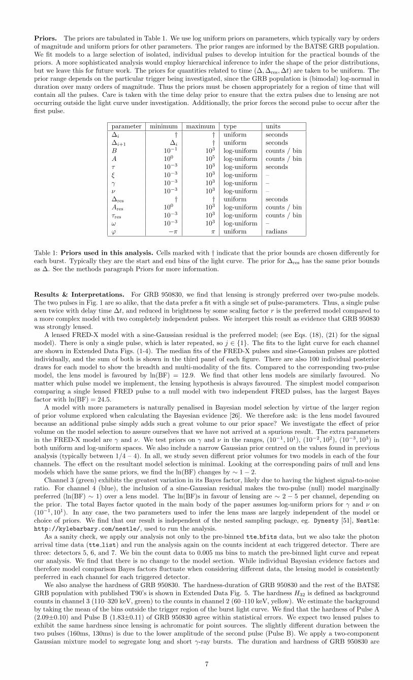
Priors. The priors are tabulated in Table 1. We use log uniform priors on parameters, which typically vary by ordersof magnitude and uniform priors for other parameters. The prior ranges are informed by the BATSE GRB population.We fit models to a large selection of isolated, individual pulses to develop intuition for the practical bounds of thepriors. A more sophisticated analysis would employ hierarchical inference to infer the shape of the prior distributions,but we leave this for future work. The priors for quantities related to time (∆,∆res,∆t) are taken to be uniform. Theprior range depends on the particular trigger being investigated, since the GRB population is (bimodal) log-normal induration over many orders of magnitude. Thus the priors must be chosen appropriately for a region of time that willcontain all the pulses. Care is taken with the time delay prior to ensure that the extra pulses due to lensing are notoccurring outside the light curve under investigation. Additionally, the prior forces the second pulse to occur after thefirst pulse.

parameter minimum maximum type units∆i † † uniform seconds∆i+1 ∆i † uniform secondsB 10−1 103 log-uniform counts / binA 100 105 log-uniform counts / binτ 10−3 103 log-uniform secondsξ 10−3 103 log-uniform –γ 10−3 103 log-uniform –ν 10−3 103 log-uniform –∆res † † uniform secondsAres 100 103 log-uniform counts / binτres 10−3 103 log-uniform counts / binω 10−3 103 log-uniform –ϕ −π π uniform radians

Table 1: Priors used in this analysis. Cells marked with † indicate that the prior bounds are chosen differently foreach burst. Typically they are the start and end bins of the light curve. The prior for ∆res has the same prior boundsas ∆. See the methods paragraph Priors for more information.

Results & Interpretations. For GRB 950830, we find that lensing is strongly preferred over two-pulse models.The two pulses in Fig. 1 are so alike, that the data prefer a fit with a single set of pulse-parameters. Thus, a single pulseseen twice with delay time ∆t, and reduced in brightness by some scaling factor r is the preferred model compared toa more complex model with two completely independent pulses. We interpret this result as evidence that GRB 950830was strongly lensed.

A lensed FRED-X model with a sine-Gaussian residual is the preferred model; (see Eqs. (18), (21) for the signalmodel). There is only a single pulse, which is later repeated, so j ∈ 1. The fits to the light curve for each channelare shown in Extended Data Figs. (1-4). The median fits of the FRED-X pulses and sine-Gaussian pulses are plottedindividually, and the sum of both is shown in the third panel of each figure. There are also 100 individual posteriordraws for each model to show the breadth and multi-modality of the fits. Compared to the corresponding two-pulsemodel, the lens model is favoured by ln(BF) = 12.9. We find that other lens models are similarly favoured. Nomatter which pulse model we implement, the lensing hypothesis is always favoured. The simplest model comparisoncomparing a single lensed FRED pulse to a null model with two independent FRED pulses, has the largest Bayesfactor with ln(BF) = 24.5.

A model with more parameters is naturally penalised in Bayesian model selection by virtue of the larger regionof prior volume explored when calculating the Bayesian evidence [26]. We therefore ask: is the lens model favouredbecause an additional pulse simply adds such a great volume to our prior space? We investigate the effect of priorvolume on the model selection to assure ourselves that we have not arrived at a spurious result. The extra parametersin the FRED-X model are γ and ν. We test priors on γ and ν in the ranges, (10−1, 101), (10−2, 102), (10−3, 103) inboth uniform and log-uniform spaces. We also include a narrow Gaussian prior centred on the values found in previousanalysis (typically between 1/4 – 4). In all, we study seven different prior volumes for two models in each of the fourchannels. The effect on the resultant model selection is minimal. Looking at the corresponding pairs of null and lensmodels which have the same priors, we find the ln(BF) changes by ∼ 1− 2.

Channel 3 (green) exhibits the greatest variation in its Bayes factor, likely due to having the highest signal-to-noiseratio. For channel 4 (blue), the inclusion of a sine-Gaussian residual makes the two-pulse (null) model marginallypreferred (ln(BF) ∼ 1) over a lens model. The ln(BF)s in favour of lensing are ∼ 2 − 5 per channel, depending onthe prior. The total Bayes factor quoted in the main body of the paper assumes log-uniform priors for γ and ν on(10−1, 101). In any case, the two parameters used to infer the lens mass are largely independent of the model orchoice of priors. We find that our result is independent of the nested sampling package, eg. Dynesty [51], Nestle:http://kylebarbary.com/nestle/, used to run the analysis.

As a sanity check, we apply our analysis not only to the pre-binned tte bfits data, but we also take the photonarrival time data (tte list) and run the analysis again on the counts incident at each triggered detector. There arethree: detectors 5, 6, and 7. We bin the count data to 0.005 ms bins to match the pre-binned light curve and repeatour analysis. We find that there is no change to the model section. While individual Bayesian evidence factors andtherefore model comparison Bayes factors fluctuate when considering different data, the lensing model is consistentlypreferred in each channel for each triggered detector.

We also analyse the hardness of GRB 950830. The hardness-duration of GRB 950830 and the rest of the BATSEGRB population with published T90’s is shown in Extended Data Fig. 5. The hardness H32 is defined as backgroundcounts in channel 3 (110–320 keV, green) to the counts in channel 2 (60–110 keV, yellow). We estimate the backgroundby taking the mean of the bins outside the trigger region of the burst light curve. We find that the hardness of Pulse A(2.09±0.10) and Pulse B (1.83±0.11) of GRB 950830 agree within statistical errors. We expect two lensed pulses toexhibit the same hardness since lensing is achromatic for point sources. The slightly different duration between thetwo pulses (160ms, 130ms) is due to the lower amplitude of the second pulse (Pulse B). We apply a two-componentGaussian mixture model to segregate long and short γ-ray bursts. The duration and hardness of GRB 950830 are

7

typical of a short gamma-ray burst. We have include the autocorrelation of the light curve of GRB 950830 in ExtendedData Fig. 6.

To improve our analysis, we could a priori constrain the magnification ratio and time delay to be the sameparameter in each of the spectral channels. The eight parameters in the lens model – two from each channel – arereduced to just two shared between the four energy channels. However, analysing the channels separately provides anindependent check that the magnification ratios and time delays are consistent, in accordance with the equivalenceprinciple (cf. Fig. 3, Extended Data Fig. 8). Below, we revisit this topic, analysing the data with multiple channelssimultaneously. Doing this four-channel nested sampling analysis on the FRED-X model with a sine-Gaussian residualbecomes prohibitively expensive. Since we believe that this will only increase the Bayesian evidence in favour oflensing, and since our result is already quite strong (ln(BF) = 12.9), we leave this analysis for future work.

Furthermore, we could include a spectral model to relate the pulse-fits in the four channels, reducing the number offree parameters in our model. The canonical GRB spectra model – the Band function – is a time averaged spectra [52],which would not suit our purposes of a time-evolving spectra. Addition of a spectral model requires the analysis offour time-series simultaneously, which is computationally challenging. We leave this as a goal for future work.

Another future goal is to use hierarchical inference to infer the prior distributions for FRED-X parameters usingthe full catalogue of GRBs, the vast majority of which do not contain a lens. This would yield priors consistent withthe population properties of GRBs. Again, we expect this to only strengthen the evidence in favour of lensing. Finally,we do not fully utilise the available high-resolution (TTE-list data), since this requires analysis of an 800,000 unittime series. This analysis is prohibitively expensive for the many-parameter models. We are able to run a simpleFRED model Eq. (17), and found that lensing was similarly favoured in all channels when running the analysis withthe pre-binned BFITS data.

We have thus-far assumed that we expect each image of a gravitationally lensed GRB will be statistically consistent.We have not discussed the many potential causes for anisotropy between the images. Gamma-ray bursts are highlybeamed due to the ultra-relativistic velocities (γ ∼ 103−4) of their progenitor outflow. This results in the viewingangle onto the emission surface becoming important, since the radiation is beamed within and angle of θ ∼ γ−1.The difference in viewing angle onto the source scales with the mass of the lens – the more massive the lens, thestronger the deflection, the greater the original angular separation of the lines-of-sight onto the source. Assuminga homogeneous emission surface, both lines-of-sight onto the source should be viewing the same region for massesMlens . 1012 M. For larger masses, the deflection angle becomes great enough such that the observer is viewingtwo emission regions which may not be in casual contact, thus the gravitationally lensed images need not be identical.For smaller lens masses, anisotropy in the GRB emission surface can result in the images having inherent differences.Finally, as discussed earlier, the detector orientation and energy response can have a significant effect on the inferredenergy spectrum, potentially resulting in a false negative identification of a gravitationally lensed pair of γ-ray bursts.

Method limitations. Our method provides advantages over model-agnostic approaches such as correlation, whichdo not include all available information, for example, Poisson counting statistics. Bayesian inference provides a naturalframework to make quantitative statistical statements about preferred models. Our methodology provides a metric fordetection significance, and successfully rejects dubious candidates, which trigger an autocorrelation detection (see Arejected candidate). Of course, the results of Bayesian inference are only as good as the choice of model and priors.We try a variety of pulse models and prior ranges to ensure our results are robust, and find that the statisticallyidentical pulse model is consistently preferred. This does not preclude the existence of a better pulse model. Wehave shown that the gravitational lens candidate GRB 950830 is robustly detected using both traditional GRB lensingtechniques and our Bayesian inference method.

Finally, we point out that any method relying on self similarity can produce false positive lensing candidatesif identical repeating pulses are a feature of some γ-ray bursts. However, we regard the “intrinsic self-similarity”hypothesis as unlikely since the vast majority of GRBs are not seen to repeat, and we cannot think of a physicalmechanism that would cause a subpopulation of short GRBs to emit identical pulses.

Estimate of Optical Depth. A rough estimate for the optical depth to strong gravitational lensing is

τ =Nlens

NGRB, (27)

where Nlens is the number of multiply-imaged GRBs and NGRB is the total number of GRBs in our dataset. We findNlens = 1 lensed GRB in a dataset of NGRB = 2, 679, so the lens probability is P (τ) ∼ τ = 3.7+7.8

−2.6 × 10−4 (90%credibility), where we have used a Jeffreys prior. We may relate the energy density of lenses to the optical depth,Ωl ∼ τ(〈zs〉) [17], where 〈zs〉 is the mean redshift of sources in the sample.

For a point mass and a point lens, the angular Einstein radius of the lens is

θ2E =

4GMl

c2dA(zl, zs)

dA(zl)dA(zs). (28)

Here, G is the gravitational constant, c the speed of light, and Ml the mass of the gravitational lens. The angulardiameter distances are defined as dA(zl, zs) = (χ(zs)− χ(zl)) /(1 + zs), with proper comoving distance

χ(zl, zs) =c

H0

∫ zs

zl

dz√ΩΛ + Ωm(1 + z)3

. (29)

We take ΩΛ = 0.714, and Ωm = 0.286, with present day Hubble constant H0 = 69.6 km s−1Mpc−1. The angularimpact parameter β of the true position of the source to the lens can be parameterised in units of the Einstein radius,y ≡ β/θE . Such a configuration creates two images, with time delay given by

∆t(Ml, zl, y) = (1 + zl)4GMl

c3f(y), (30)

where

f(y) =

(y

2

√y2 + 4 + ln

√y2 + 4 + y√y2 + 4− y

.

)(31)

8

A source with angular impact parameter β has an effective lensing cross-section of∫σ =

∫ βmax

βmin

2πβ dβ

= πθ2E

∫ ymax

ymin

2ydy

=4πGMl

c2dA(zl, zs)

dA(zl)dA(zs)

∫ ymax

ymin

2y dy. (32)

Thus, ymin and ymax turn the cross-section into an annulus. The minimum impact parameter is set by the time delaybetween the arrival times of the two images. If the time delay is too short, the images will appear as single gamma-rayburst. For a point lens, we may calculate the minimum time delay for a lens of mass Ml at redshift zl by invertingequation (30),

ymin(∆tmin,Ml, zl) = f−1

(c3∆tmin

(1 + zl)4GMl

), (33)

since f(y) is monotonic increasing in y. We take ∆tmin = 10 ms. The latter-arriving image is dimmer than the firstimage but must still be above the detectable flux for the detector, µ2ϕpeak > ϕ0, where µ2 is the magnification of thedimmer image. This restricts the maximum possible impact parameter [23]:

ymax(ϕpeak) =

(1 +

ϕpeak

ϕ0

)1/4

−(

1 +ϕpeak

ϕ0

)−1/4

, (34)

where ϕpeak/ϕ0 is the peak counts divided by the trigger threshold at that time. We estimate ymax with medi-ans of the ϕpeak/ϕ0 for the peak flux on 64 ms, 256 ms, and 1024 ms integrations from the BATSE Cmax table:https://gammaray.nsstc.nasa.gov/batse/grb/catalog/4b/tables/4br_grossc.cmaxmin, which are 1.5, 2.2, and2.5 respectively. The final cross section is then

σ(~x) =4πGMl

c2dA(zl)dA(zl, zs)

dA(zs)

(y2

max − y2min

)Θ (ymax − ymin) (35)

where ~x ≡ (Ml, zl, zs, ϕpeak, ϕ0,∆tmin) and Θ is the Heaviside step function.The optical depth is the number density n(zl) of lenses at redshift zl, multiplied by the effective lensing cross-section

of each lens σ(~x), integrated over z ∈ (0, zs):

τ(~x) =1

dΩ

∫ zs

0

dV (zl)n(zl)

∫dσ(~x). (36)

We assume a constant comoving density of lenses,

nl(zl) = n0(1 + zl)3. (37)

The number density of lenses can be related to their energy density Ωl through

n0 =ρcΩlMl

=3H2

0 Ωl8πGMl

. (38)

With comoving volume element

dV (z) = χ2(z)dχ(z)

dzdzdΩ

= χ2(z)c

H0

dz dΩ√ΩΛ + Ωm(1 + z)3

, (39)

we have

τ(~x) =3H0Ωl2cχ(zs)

∫ zs

0

dzl(1 + zl)χ(zl)√

ΩΛ + Ωm(1 + zl)3[χ(zs)− χ(zl)]

·[y2

max(ϕpeak, ϕ0)− y2min(∆tmin,Ml, zl)

]. (40)

With an estimated lens probability of P (τ) ∼ τ ≈ 3.7× 10−4, we infer the lens density by inversion of Eq. (40). Theresult of this integral is shown in Extended Data Fig. 9 for several mean source redshifts 〈zs〉 each with the threepermutations of ϕpeak/ϕ0 from the BATSE Cmax table.

The 7 BATSE bursts with known redshifts are GRB 970508: z = 0.835, GRB 970828: z = 0.958, GRB 971214:z = 3.412, GRB 980425: z = 0.0085, GRB 980703: z = 0.967, GRB 990123: z = 1.600, GRB 990510: z = 1.619, withmean 〈z〉 = 1.34. The average spectroscopic redshift of Swift γ-ray bursts is 〈z〉 = 2.2 [53]. We are unable to accuratelyestimate the redshift of GRB 950830 or the BATSE catalogue in general due to the inherent degeneracy between theeffects of cosmological redshift and relativistic beaming on a γ-ray burst light curve. We argue that a mean BATSEGRB redshift of 〈zs〉 ∼ 2 is appropriate based on the redshifts of known BATSE bursts and the spectroscopicallydetermined redshifts of other GRB catalogues. We include the derived energy densities for a number of redshifts inExtended Data Fig. 10 for the comparison. The lens densities are calculated from the source redshifts and opticaldepth through Eq. (40). With the inferred lens densities Ωl, we may exclude our calculated globular cluster densityΩgc ∼ 8 × 10−6 based on Poisson statistics. Observing one gravitational lens in ∼ 2, 679 light curves is very unlikelyfor such a low cosmological density.

The present day number density is given by

nimbh(zl, zs) =Ωimbh(zs) ρcMimbh(zl)

, (41)

9

where ρc is the critical energy density of the Universe and Mimbh(zl) is the mass of the lens. With Ωimbh(〈zs〉 ∼2) = 4.6+9.8

−3.3 × 10−4, and (1 + zl)Mimbh = 5.5+1.7−0.9 × 104 M =⇒ Mimbh(zl ∼ 1) ∼ 2.8+1.7

−0.9 × 104 M yields

nimbh = 2.3+4.9−1.6 × 103 Mpc−3 through Eq. (38). Where zl ∼ 1 comes from a gravitational lens being most likely to

occur halfway between the observer and source. Uncertainty on the density of IMBHs arises from the fact that Nlens

is Poisson distributed. We calculate the uncertainty on nl assuming zl = 0, as we do not know where the lens is, onlythat its most probable redshift is zl ∼ 1. We ignore the uncertainty due to the lens mass as it is much more preciselydetermined. In order to calculate the uncertainty on nimbh, we assume that the likelihood of the data given nimbhfollows an N = 1 Poisson distribution. Employing a Jeffreys’ prior,

π(nimbh ∝ n−1/2imbh ), (42)

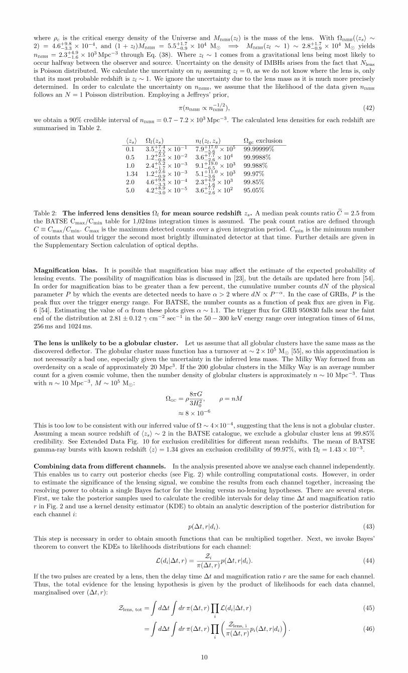
we obtain a 90% credible interval of nimbh = 0.7− 7.2× 103 Mpc−3. The calculated lens densities for each redshift aresummarised in Table 2.

〈zs〉 Ωl(zs) nl(zl, zs) Ωgc exclusion

0.1 3.5+7.4−2.5 × 10−1 7.9+17.0

−5.6 × 105 99.99999%0.5 1.2+2.5

−0.8 × 10−2 3.6+7.7−2.6 × 104 99.9988%

1.0 2.4+5.2−1.7 × 10−3 9.1+19.0

−6.5 × 103 99.988%1.34 1.2+2.6

−0.9 × 10−3 5.1+11.0−3.6 × 103 99.97%

2.0 4.6+9.8−3.3 × 10−4 2.3+4.9

−1.6 × 103 99.85%5.0 4.2+8.9

−3.0 × 10−5 3.6+7.7−2.6 × 102 95.05%

Table 2: The inferred lens densities Ωl for mean source redshift zs. A median peak counts ratio C = 2.5 fromthe BATSE Cmax/Cmin table for 1,024ms integration times is assumed. The peak count ratios are defined throughC ≡ Cmax/Cmin. Cmax is the maximum detected counts over a given integration period. Cmin is the minimum numberof counts that would trigger the second most brightly illuminated detector at that time. Further details are given inthe Supplementary Section calculation of optical depths.

Magnification bias. It is possible that magnification bias may affect the estimate of the expected probability oflensing events. The possibility of magnification bias is discussed in [23], but the details are updated here from [54].In order for magnification bias to be greater than a few percent, the cumulative number counts dN of the physicalparameter P by which the events are detected needs to have α > 2 where dN ∝ P−α. In the case of GRBs, P is thepeak flux over the trigger energy range. For BATSE, the number counts as a function of peak flux are given in Fig.6 [54]. Estimating the value of α from these plots gives α ∼ 1.1. The trigger flux for GRB 950830 falls near the faintend of the distribution at 2.81± 0.12 γ cm−2 sec−1 in the 50− 300 keV energy range over integration times of 64 ms,256 ms and 1024 ms.

The lens is unlikely to be a globular cluster. Let us assume that all globular clusters have the same mass as thediscovered deflector. The globular cluster mass function has a turnover at ∼ 2× 105 M [55], so this approximation isnot necessarily a bad one, especially given the uncertainty in the inferred lens mass. The Milky Way formed from anoverdensity on a scale of approximately 20 Mpc3. If the 200 globular clusters in the Milky Way is an average numbercount for a given cosmic volume, then the number density of globular clusters is approximately n ∼ 10 Mpc−3. Thuswith n ∼ 10 Mpc−3, M ∼ 105 M:

Ωgc = ρ8πG

3H20

, ρ = nM

≈ 8× 10−6

This is too low to be consistent with our inferred value of Ω ∼ 4×10−4, suggesting that the lens is not a globular cluster.Assuming a mean source redshift of 〈zs〉 ∼ 2 in the BATSE catalogue, we exclude a globular cluster lens at 99.85%credibility. See Extended Data Fig. 10 for exclusion credibilities for different mean redshifts. The mean of BATSEgamma-ray bursts with known redshift 〈z〉 = 1.34 gives an exclusion credibility of 99.97%, with Ωl = 1.43× 10−3.

Combining data from different channels. In the analysis presented above we analyse each channel independently.This enables us to carry out posterior checks (see Fig. 2) while controlling computational costs. However, in orderto estimate the significance of the lensing signal, we combine the results from each channel together, increasing theresolving power to obtain a single Bayes factor for the lensing versus no-lensing hypotheses. There are several steps.First, we take the posterior samples used to calculate the credible intervals for delay time ∆t and magnification ratior in Fig. 2 and use a kernel density estimator (KDE) to obtain an analytic description of the posterior distribution foreach channel i:

p(∆t, r|di). (43)

This step is necessary in order to obtain smooth functions that can be multiplied together. Next, we invoke Bayes’theorem to convert the KDEs to likelihoods distributions for each channel:

L(di|∆t, r) =Zi

π(∆t, r)p(∆t, r|di). (44)

If the two pulses are created by a lens, then the delay time ∆t and magnification ratio r are the same for each channel.Thus, the total evidence for the lensing hypothesis is given by the product of likelihoods for each data channel,marginalised over (∆t, r):

Zlens, tot =

∫d∆t

∫dr π(∆t, r)

∏i

L(di|∆t, r) (45)

=

∫d∆t

∫dr π(∆t, r)

∏i

(Zlens, i

π(∆t, r)pi(∆t, r|di)

). (46)

10

On the other hand, if the two pulses are not created from a lens, there is no reason for the delay time and magnificationratio to be the same for each channel, and so the total evidence for the null hypothesis is given simply by the productof the evidence values for each channel:

Ztotnull =

∏i

Znull, i (47)

Evaluating Eqs. 45 and 47, we obtain a total Bayes factor ln(BF) = 12.93 in favour of the lensing hypothesis.

False alarm probability. In Bayesian statistics, we carry out model selection using the posterior odds [26],

Olensnull =

Zlens

Znull

πlens

πnull, (48)

where Zlens/Znull = BF is the Bayes factor from Eq. (26). The prior odds, πlens/πnull, expresses the relative probabilityassigned a priori to the hypothesis of lensing over a null model. If we assign an equal prior probability to bothhypotheses, then

Olensnull =

Zlens

Znull(49)

=plens

1− plens, (50)

and so the false alarm probability is

1− plens =1

1 + BF

=1

1 + e12.9

= 2.5× 10−6

A more conservative approach is to assign prior odds equal to the reciprocal of the total number of bursts searched(or equivalently, equal to the optical depth), which gives us:

Olensnull =

Zlens

Znull

πlens

πnull

=BF

2, 679,

which gives a false alarm probability of

1− plens =1

1 + BF/2, 679

=1

1 + e12.9/2, 679

= 6.5× 10−3.

We see that the strong preference for the lensing hypothesis persists even taking into account trial factors.

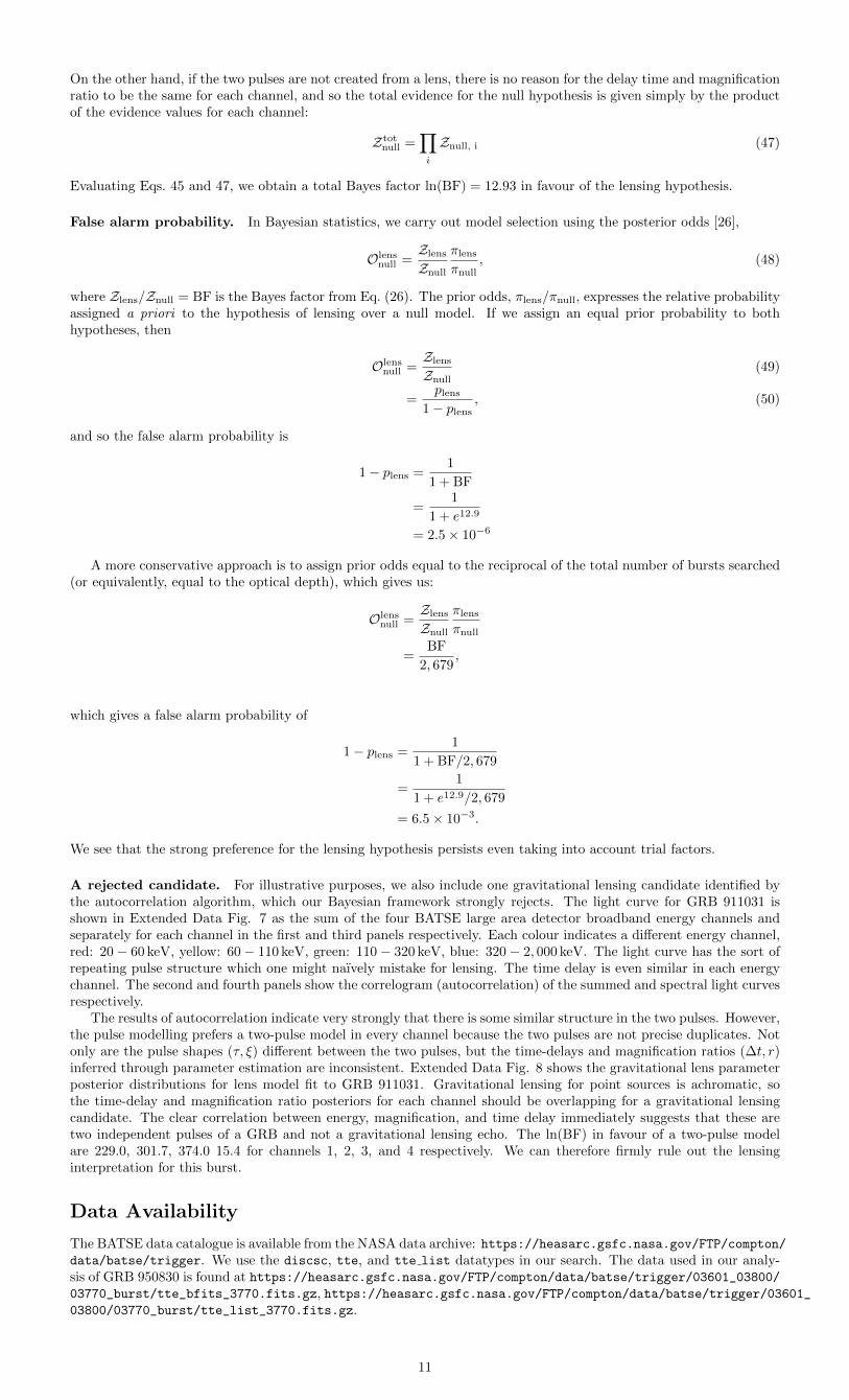
A rejected candidate. For illustrative purposes, we also include one gravitational lensing candidate identified bythe autocorrelation algorithm, which our Bayesian framework strongly rejects. The light curve for GRB 911031 isshown in Extended Data Fig. 7 as the sum of the four BATSE large area detector broadband energy channels andseparately for each channel in the first and third panels respectively. Each colour indicates a different energy channel,red: 20 − 60 keV, yellow: 60 − 110 keV, green: 110− 320 keV, blue: 320− 2, 000 keV. The light curve has the sort ofrepeating pulse structure which one might naıvely mistake for lensing. The time delay is even similar in each energychannel. The second and fourth panels show the correlogram (autocorrelation) of the summed and spectral light curvesrespectively.

The results of autocorrelation indicate very strongly that there is some similar structure in the two pulses. However,the pulse modelling prefers a two-pulse model in every channel because the two pulses are not precise duplicates. Notonly are the pulse shapes (τ, ξ) different between the two pulses, but the time-delays and magnification ratios (∆t, r)inferred through parameter estimation are inconsistent. Extended Data Fig. 8 shows the gravitational lens parameterposterior distributions for lens model fit to GRB 911031. Gravitational lensing for point sources is achromatic, sothe time-delay and magnification ratio posteriors for each channel should be overlapping for a gravitational lensingcandidate. The clear correlation between energy, magnification, and time delay immediately suggests that these aretwo independent pulses of a GRB and not a gravitational lensing echo. The ln(BF) in favour of a two-pulse modelare 229.0, 301.7, 374.0 15.4 for channels 1, 2, 3, and 4 respectively. We can therefore firmly rule out the lensinginterpretation for this burst.

Data Availability

The BATSE data catalogue is available from the NASA data archive: https://heasarc.gsfc.nasa.gov/FTP/compton/data/batse/trigger. We use the discsc, tte, and tte list datatypes in our search. The data used in our analy-sis of GRB 950830 is found at https://heasarc.gsfc.nasa.gov/FTP/compton/data/batse/trigger/03601_03800/03770_burst/tte_bfits_3770.fits.gz, https://heasarc.gsfc.nasa.gov/FTP/compton/data/batse/trigger/03601_03800/03770_burst/tte_list_3770.fits.gz.

11

Code Availability

The analysis code PyGRB [56] has been written in python [57] by J.P. and is freely available at https://github.

com/JamesPaynter/PyGRB under the BSD 3-Clause License. PyGRB is built around Monash University’s Bilby nestedsampling wrapper, with additional FITS I/O functionality provided by AstroPy [58]. The software uses the NumPy [59]and SciPy [60] computational libraries. Plotting makes use of the Matplotlib [61] and corner [62] libraries.

References

[31] G. F. Marani, R. J. Nemiroff, J. P. Norris, K. Hurley, and J. T. Bonnell. Gravitationally Lensed Gamma-RayBursts as Probes of Dark Compact Objects. Astrophys. J. Lett., 512(1):L13–L16, 1999.

[32] L. L. R. Williams and R. A. M. J. Wijers. Distortion of gamma-ray burst light curves by gravitational microlensing.Mon. Not. R. Ast. Soc., 286(1):L11–L16, 1997.

[33] J. S. B. Wyithe and E. L. Turner. Gravitational microlensing of gamma-ray bursts at medium optical depth.Mon. Not. R. Ast. Soc., 319(4):1163–1168, 2000.

[34] Geraint F Lewis. Gravitational microlensing time delays at high optical depth: image parities and the temporalproperties of fast radio bursts. Mon. Not. R. Ast. Soc., 497(2):1583–1589, 2020.

[35] Mark A. Walker and Geraint F. Lewis. Nanolensing of Gamma-Ray Bursts. Astrophys. J., 589(2):844–860, 2003.

[36] Andrew Gould. Femtolensing of Gamma-Ray Bursters. Astrophys. J. Lett., 386:L5–L7, 1992.

[37] R. J. Nemiroff, J. P. Norris, W. A. D. T. Wickramasinghe, J. M. Horack, C. Kouveliotou, G. J. Fishman,C. A. Meegan, R. B. Wilson, and W. S. Paciesas. Searching gamma-ray bursts for gravitational lensing echoes -Implications for compact dark matter. Astrophys. J., 414:36–40, 1993.

[38] O. S. Ougolnikov. A Search for Possible Mesolensing of Cosmic Gamma-Ray Bursts: II. Double and Triple Burstsin the BATSE Catalog. Cosmic Research, 41(2):141–146, 2003.

[39] B. Biltzinger, F. Kunzweiler, J. Greiner, K. Toelge, and J. Michael Burgess. A physical background model for theFermi Gamma-ray Burst Monitor. Astron. Astrophys., 640:A8, 2020.

[40] Robert J. Nemiroff, Gabriela F. Marani, Jay P. Norris, Jerry T. Bonnell, Charles A. Meegan, and Kevin C.Hurley. Gamma-ray burst lensing limits on cosmological parameters. In R. Marc Kippen, Robert S. Mallozzi, andGerald J. Fishman, editors, Gamma-ray Bursts, 5th Huntsville Symposium, volume 526 of American Institute ofPhysics Conference Series, pages 663–667, 2000.

[41] C. Li and L. Li. Search for strong gravitational lensing effect in the current GRB data of BATSE. Science ChinaPhysics, Mechanics, and Astronomy, 57:1592–1599, 2014.

[42] R. Davidson, P. N. Bhat, and G. Li. Are there Gravitationally Lensed Gamma-ray Bursts detected by GBM? InJ. E. McEnery, J. L. Racusin, and N. Gehrels, editors, American Institute of Physics Conference Series, volume1358 of American Institute of Physics Conference Series, pages 17–20, 2011.

[43] Zsolt Bagoly and Peter Veres. Achromatic Search for Gravitational Lensing in Fermi Data. In Nobuyuki Kawaiand Shigehiro Nagataki, editors, American Institute of Physics Conference Series, volume 1279 of AmericanInstitute of Physics Conference Series, pages 293–295, 2010.

[44] Masamune Oguri. Strong gravitational lensing of explosive transients. Reports on Progress in Physics,82(12):126901, 2019.

[45] Jon Hakkila, Istvan Horvath, Eric Hofesmann, and Stephen Lesage. Properties of Short Gamma-ray Burst Pulsesfrom a BATSE TTE GRB Pulse Catalog. Astrophys. J., 855(2):101, 2018.

[46] Gregory Ashton, Moritz Hubner, Paul D. Lasky, Colm Talbot, Kendall Ackley, Sylvia Biscoveanu, Qi Chu, AtulDivakarla, Paul J. Easter, Boris Goncharov, Francisco Hernandez Vivanco, Jan Harms, Marcus E. Lower, GrantD. Meadors, Denyz Melchor, Ethan Payne, Matthew D. Pitkin, Jade Powell, Nikhil Sarin, Rory J.E. Smith, andEric Thrane. Bilby: A user-friendly bayesian inference library for gravitational-wave astronomy. The AstrophysicalJournal Supplement Series, 241(2):27, 2019.

[47] John Skilling. Nested Sampling. In Rainer Fischer, Roland Preuss, and Udo Von Toussaint, editors, AmericanInstitute of Physics Conference Series, volume 735 of American Institute of Physics Conference Series, pages395–405, 2004.

[48] John Skilling. Nested sampling for general bayesian computation. Bayesian Anal., 1(4):833–859, 2006.

[49] F. Feroz, M. P. Hobson, and M. Bridges. MULTINEST: an efficient and robust Bayesian inference tool forcosmology and particle physics. Mon. Not. R. Ast. Soc., 398(4):1601–1614, 2009.

[50] Edward Higson, Will Handley, Mike Hobson, and Anthony Lasenby. Dynamic nested sampling: an improvedalgorithm for parameter estimation and evidence calculation. Statistics and Computing, 29(5):891–913, 2019.

[51] Joshua S. Speagle. DYNESTY: a dynamic nested sampling package for estimating Bayesian posteriors andevidences. Mon. Not. R. Ast. Soc., 493(3):3132–3158, 2020.

[52] D. Band, J. Matteson, L. Ford, B. Schaefer, D. Palmer, B. Teegarden, T. Cline, M. Briggs, W. Paciesas, G. Pendle-ton, G. Fishman, C. Kouveliotou, C. Meegan, R. Wilson, and P. Lestrade. BATSE Observations of Gamma-RayBurst Spectra. I. Spectral Diversity. Astrophys. J., 413:281–292, 1993.

12

[53] Limin Xiao and Bradley E. Schaefer. Redshift Catalog for Swift Long Gamma-ray Bursts. Astrophys. J.,731(2):103, 2011.

[54] William S. Paciesas, Charles A. Meegan, Geoffrey N. Pendleton, Michael S. Briggs, Chryssa Kouveliotou,Thomas M. Koshut, John Patrick Lestrade, Michael L. McCollough, Jerome J. Brainerd, Jon Hakkila, WilliamHenze, Robert D. Preece, Valerie Connaughton, R. Marc Kippen, Robert S. Mallozzi, Gerald J. Fishman, Geor-gia A. Richardson, and Maitrayee Sahi. The Fourth BATSE Gamma-Ray Burst Catalog (Revised). Astrophys. J.Supp., 122(2):465–495, 1999.

[55] Andres Jordan, Dean E. McLaughlin, Patrick Cote, Laura Ferrarese, Eric W. Peng, Simona Mei, Daniela Villegas,David Merritt, John L. Tonry, and Michael J. West. The ACS Virgo Cluster Survey. XII. The Luminosity Functionof Globular Clusters in Early-Type Galaxies. Astrophys. J. Supp., 171(1):101–145, 2007.

[56] James R. Paynter. Pygrb: A pure python gamma-ray burst analysis package. Journal of Open Source Software,5(53):2536, 2020.

[57] Guido Van Rossum and Fred L. Drake. Python 3 Reference Manual. CreateSpace, Scotts Valley, CA, 2009.

[58] Astropy Collaboration, T. P. Robitaille, E. J. Tollerud, P. Greenfield, M. Droettboom, E. Bray, T. Aldcroft,M. Davis, A. Ginsburg, A. M. Price-Whelan, W. E. Kerzendorf, A. Conley, N. Crighton, K. Barbary, D. Muna,H. Ferguson, F. Grollier, M. M. Parikh, P. H. Nair, H. M. Unther, C. Deil, J. Woillez, S. Conseil, R. Kramer,J. E. H. Turner, L. Singer, R. Fox, B. A. Weaver, V. Zabalza, Z. I. Edwards, K. Azalee Bostroem, D. J. Burke,A. R. Casey, S. M. Crawford, N. Dencheva, J. Ely, T. Jenness, K. Labrie, P. L. Lim, F. Pierfederici, A. Pontzen,A. Ptak, B. Refsdal, M. Servillat, and O. Streicher. Astropy: A community Python package for astronomy.Astron. Astrophys., 558:A33, 2013.

[59] S. van der Walt, S. C. Colbert, and G. Varoquaux. The numpy array: A structure for efficient numericalcomputation. Computing in Science Engineering, 13(2):22–30, 2011.

[60] Pauli Virtanen, Ralf Gommers, Travis E. Oliphant, Matt Haberland, Tyler Reddy, David Cournapeau, EvgeniBurovski, Pearu Peterson, Warren Weckesser, Jonathan Bright, Stefan J. van der Walt, Matthew Brett, JoshuaWilson, K. Jarrod Millman, Nikolay Mayorov, Andrew R. J. Nelson, Eric Jones, Robert Kern, Eric Larson,CJ Carey, Ilhan Polat, Yu Feng, Eric W. Moore, Jake VanderPlas, Denis Laxalde, Josef Perktold, Robert Cimr-man, Ian Henriksen, E. A. Quintero, Charles R Harris, Anne M. Archibald, Antonio H. Ribeiro, Fabian Pedregosa,Paul van Mulbregt, and SciPy 1. 0 Contributors. SciPy 1.0: Fundamental Algorithms for Scientific Computingin Python. Nature Methods, 17:261–272, 2020.

[61] J. D. Hunter. Matplotlib: A 2d graphics environment. Computing in Science & Engineering, 9(3):90–95, 2007.

[62] Daniel Foreman-Mackey. corner.py: Scatterplot matrices in python. The Journal of Open Source Software, 1:24,2016.

[63] Bernard Meade, Lev Lafayette, Greg Sauter, and Daniel Tosello. Spartan HPC-Cloud Hybrid: Deliver-ing Performance and Flexibility. https://melbourne.figshare.com/articles/Spartan_HPC-Cloud_Hybrid_

Delivering_Performance_and_Flexibility/4768291, 2017.

13

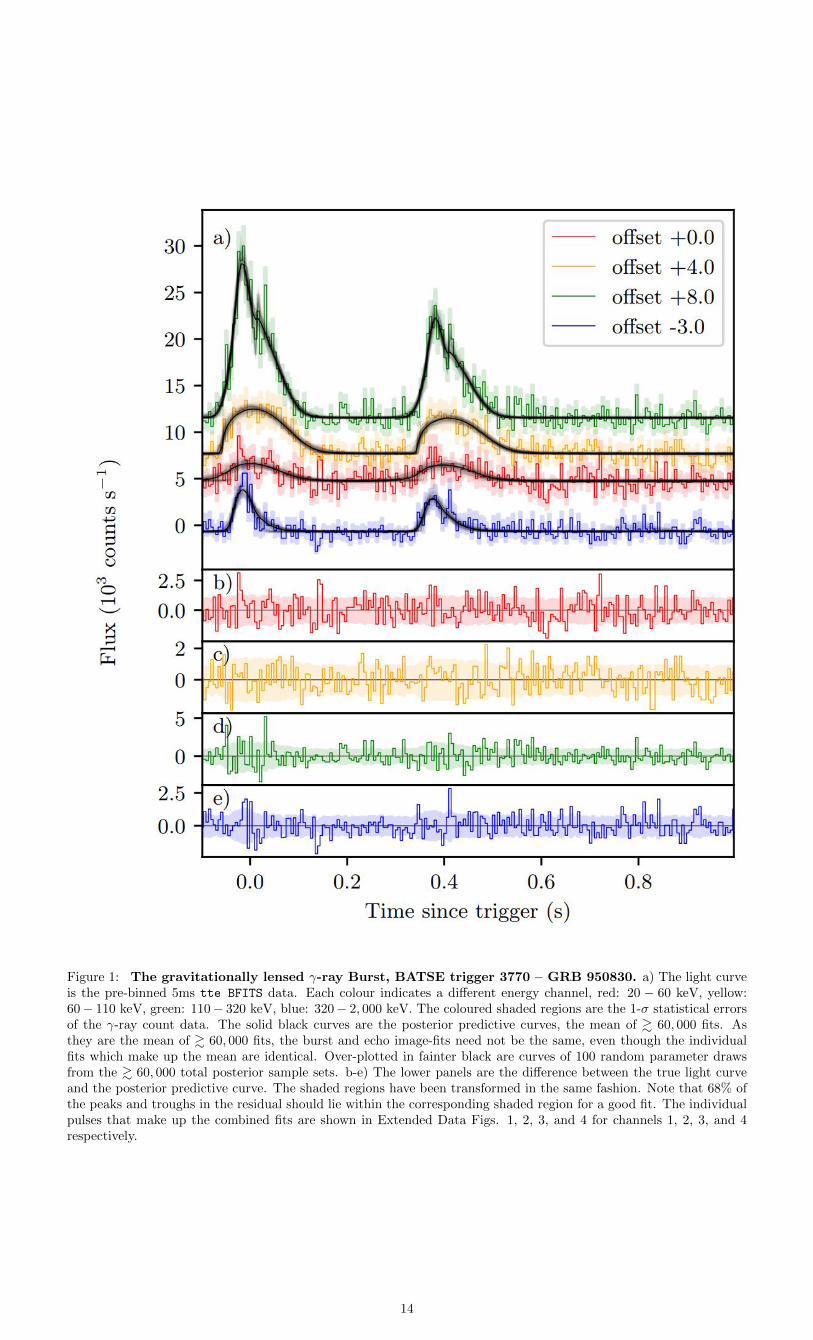
Figure 1: The gravitationally lensed γ-ray Burst, BATSE trigger 3770 – GRB 950830. a) The light curveis the pre-binned 5ms tte BFITS data. Each colour indicates a different energy channel, red: 20 − 60 keV, yellow:60− 110 keV, green: 110− 320 keV, blue: 320− 2, 000 keV. The coloured shaded regions are the 1-σ statistical errorsof the γ-ray count data. The solid black curves are the posterior predictive curves, the mean of & 60, 000 fits. Asthey are the mean of & 60, 000 fits, the burst and echo image-fits need not be the same, even though the individualfits which make up the mean are identical. Over-plotted in fainter black are curves of 100 random parameter drawsfrom the & 60, 000 total posterior sample sets. b-e) The lower panels are the difference between the true light curveand the posterior predictive curve. The shaded regions have been transformed in the same fashion. Note that 68% ofthe peaks and troughs in the residual should lie within the corresponding shaded region for a good fit. The individualpulses that make up the combined fits are shown in Extended Data Figs. 1, 2, 3, and 4 for channels 1, 2, 3, and 4respectively.

14

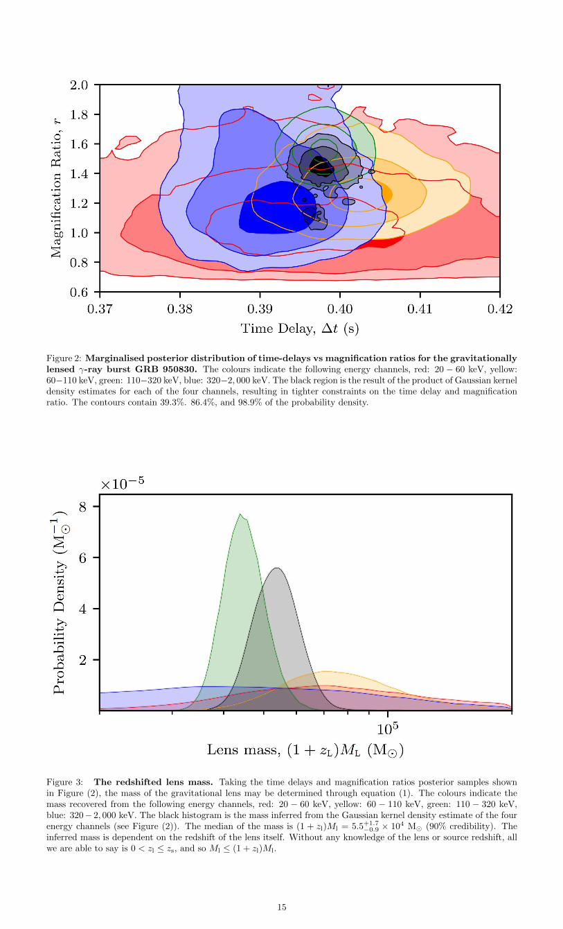
Figure 2: Marginalised posterior distribution of time-delays vs magnification ratios for the gravitationallylensed γ-ray burst GRB 950830. The colours indicate the following energy channels, red: 20 − 60 keV, yellow:60−110 keV, green: 110−320 keV, blue: 320−2, 000 keV. The black region is the result of the product of Gaussian kerneldensity estimates for each of the four channels, resulting in tighter constraints on the time delay and magnificationratio. The contours contain 39.3%. 86.4%, and 98.9% of the probability density.

Figure 3: The redshifted lens mass. Taking the time delays and magnification ratios posterior samples shownin Figure (2), the mass of the gravitational lens may be determined through equation (1). The colours indicate themass recovered from the following energy channels, red: 20 − 60 keV, yellow: 60 − 110 keV, green: 110 − 320 keV,blue: 320− 2, 000 keV. The black histogram is the mass inferred from the Gaussian kernel density estimate of the fourenergy channels (see Figure (2)). The median of the mass is (1 + zl)Ml = 5.5+1.7

−0.9 × 104 M (90% credibility). Theinferred mass is dependent on the redshift of the lens itself. Without any knowledge of the lens or source redshift, allwe are able to say is 0 < zl ≤ zs, and so Ml ≤ (1 + zl)Ml.

15

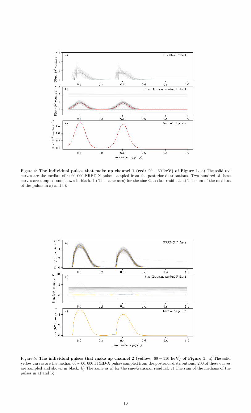
Figure 4: The individual pulses that make up channel 1 (red: 20 − 60 keV) of Figure 1. a) The solid redcurves are the median of ∼ 60, 000 FRED-X pulses sampled from the posterior distributions. Two hundred of thesecurves are sampled and shown in black. b) The same as a) for the sine-Gaussian residual. c) The sum of the mediansof the pulses in a) and b).

Figure 5: The individual pulses that make up channel 2 (yellow: 60 − 110 keV) of Figure 1. a) The solidyellow curves are the median of ∼ 60, 000 FRED-X pulses sampled from the posterior distributions. 200 of these curvesare sampled and shown in black. b) The same as a) for the sine-Gaussian residual. c) The sum of the medians of thepulses in a) and b).

16

Figure 6: The individual pulses that make up channel 3 (green: 110 − 320 keV) of Figure 1. a) The solidgreen curves are the median of ∼ 60, 000 FRED-X pulses sampled from the posterior distributions. 200 of these curvesare sampled and shown in black. b) The same as a) for the sine-Gaussian residual. c) The sum of the medians of thepulses in a) and b).

Figure 7: The individual pulses that make up channel 4 (blue: 320− 2, 000 keV) of Figure 1. a) The solidblue curves are the median of ∼ 60, 000 FRED-X pulses sampled from the posterior distributions. 200 of these curvesare sampled and shown in black. b) The same as a) for the sine-Gaussian residual. c) The sum of the medians of thepulses in a) and b).

17

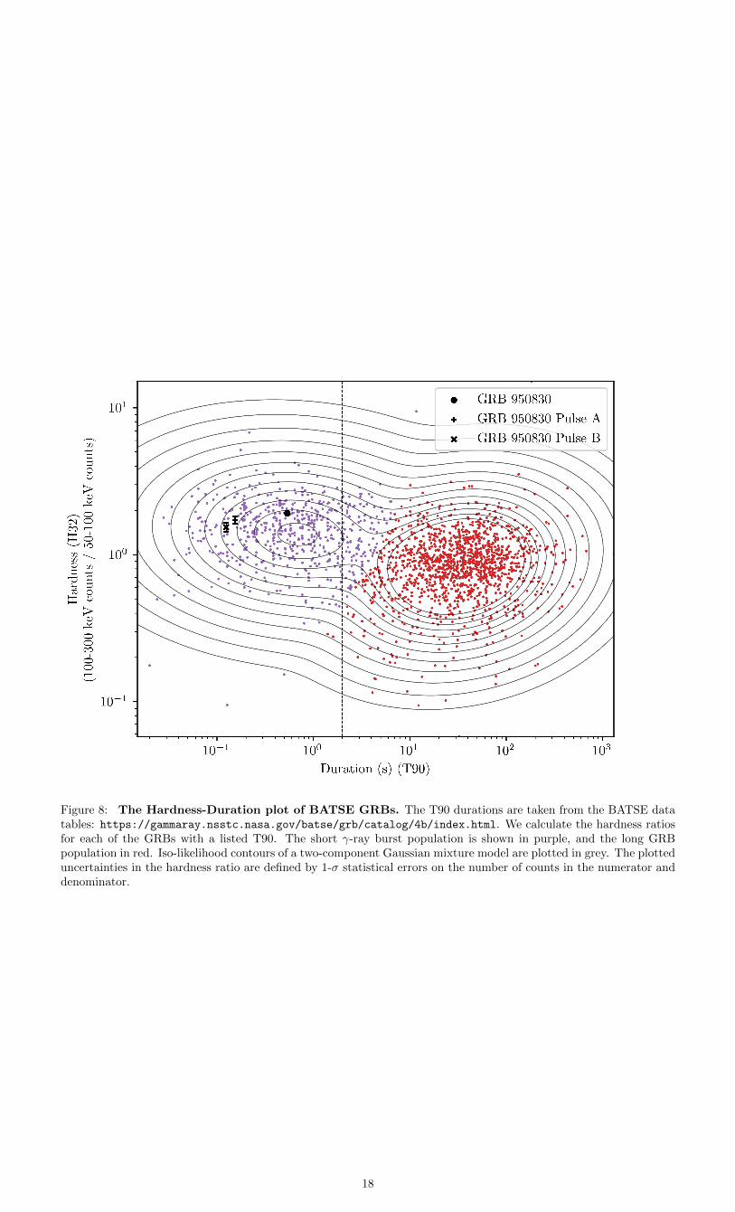
Figure 8: The Hardness-Duration plot of BATSE GRBs. The T90 durations are taken from the BATSE datatables: https://gammaray.nsstc.nasa.gov/batse/grb/catalog/4b/index.html. We calculate the hardness ratiosfor each of the GRBs with a listed T90. The short γ-ray burst population is shown in purple, and the long GRBpopulation in red. Iso-likelihood contours of a two-component Gaussian mixture model are plotted in grey. The plotteduncertainties in the hardness ratio are defined by 1-σ statistical errors on the number of counts in the numerator anddenominator.

18

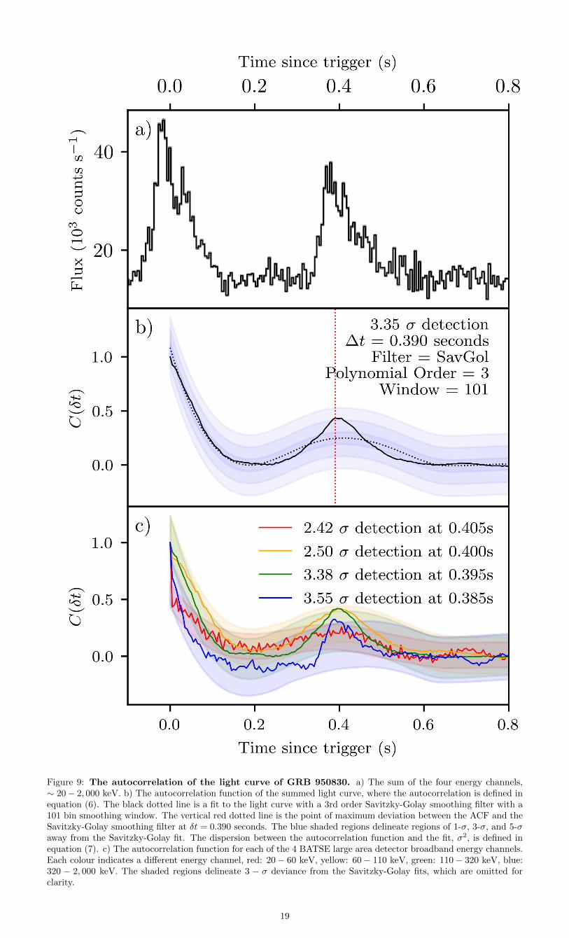
Figure 9: The autocorrelation of the light curve of GRB 950830. a) The sum of the four energy channels,∼ 20− 2, 000 keV. b) The autocorrelation function of the summed light curve, where the autocorrelation is defined inequation (6). The black dotted line is a fit to the light curve with a 3rd order Savitzky-Golay smoothing filter with a101 bin smoothing window. The vertical red dotted line is the point of maximum deviation between the ACF and theSavitzky-Golay smoothing filter at δt = 0.390 seconds. The blue shaded regions delineate regions of 1-σ, 3-σ, and 5-σaway from the Savitzky-Golay fit. The dispersion between the autocorrelation function and the fit, σ2, is defined inequation (7). c) The autocorrelation function for each of the 4 BATSE large area detector broadband energy channels.Each colour indicates a different energy channel, red: 20− 60 keV, yellow: 60− 110 keV, green: 110− 320 keV, blue:320 − 2, 000 keV. The shaded regions delineate 3 − σ deviance from the Savitzky-Golay fits, which are omitted forclarity.

19

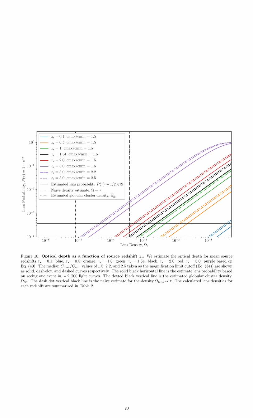
Figure 10: Optical depth as a function of source redshift zs. We estimate the optical depth for mean sourceredshifts zs = 0.1: blue, zs = 0.5: orange, zs = 1.0: green, zs = 1.34: black, zs = 2.0: red, zs = 5.0: purple based onEq. (40). The median Cmax/Cmin values of 1.5, 2.2, and 2.5 taken as the magnification limit cutoff (Eq. (34)) are shownas solid, dash-dot, and dashed curves respectively. The solid black horizontal line is the estimate lens probability basedon seeing one event in ∼ 2, 700 light curves. The dotted black vertical line is the estimated globular cluster density,Ωgc. The dash dot vertical black line is the naıve estimate for the density Ωlens ∼ τ . The calculated lens densities foreach redshift are summarised in Table 2.

20

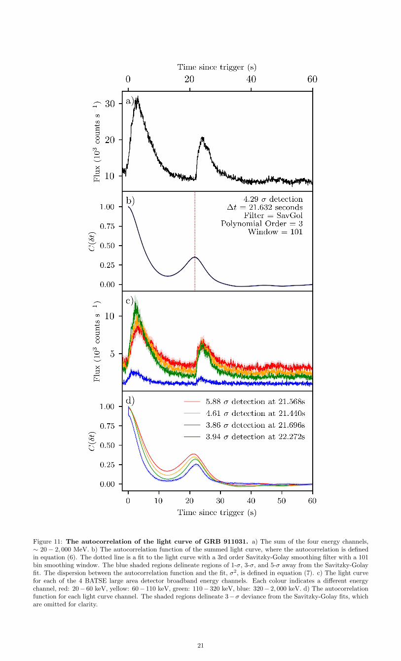
Figure 11: The autocorrelation of the light curve of GRB 911031. a) The sum of the four energy channels,∼ 20 − 2, 000 MeV. b) The autocorrelation function of the summed light curve, where the autocorrelation is definedin equation (6). The dotted line is a fit to the light curve with a 3rd order Savitzky-Golay smoothing filter with a 101bin smoothing window. The blue shaded regions delineate regions of 1-σ, 3-σ, and 5-σ away from the Savitzky-Golayfit. The dispersion between the autocorrelation function and the fit, σ2, is defined in equation (7). c) The light curvefor each of the 4 BATSE large area detector broadband energy channels. Each colour indicates a different energychannel, red: 20− 60 keV, yellow: 60− 110 keV, green: 110− 320 keV, blue: 320− 2, 000 keV. d) The autocorrelationfunction for each light curve channel. The shaded regions delineate 3−σ deviance from the Savitzky-Golay fits, whichare omitted for clarity.

21

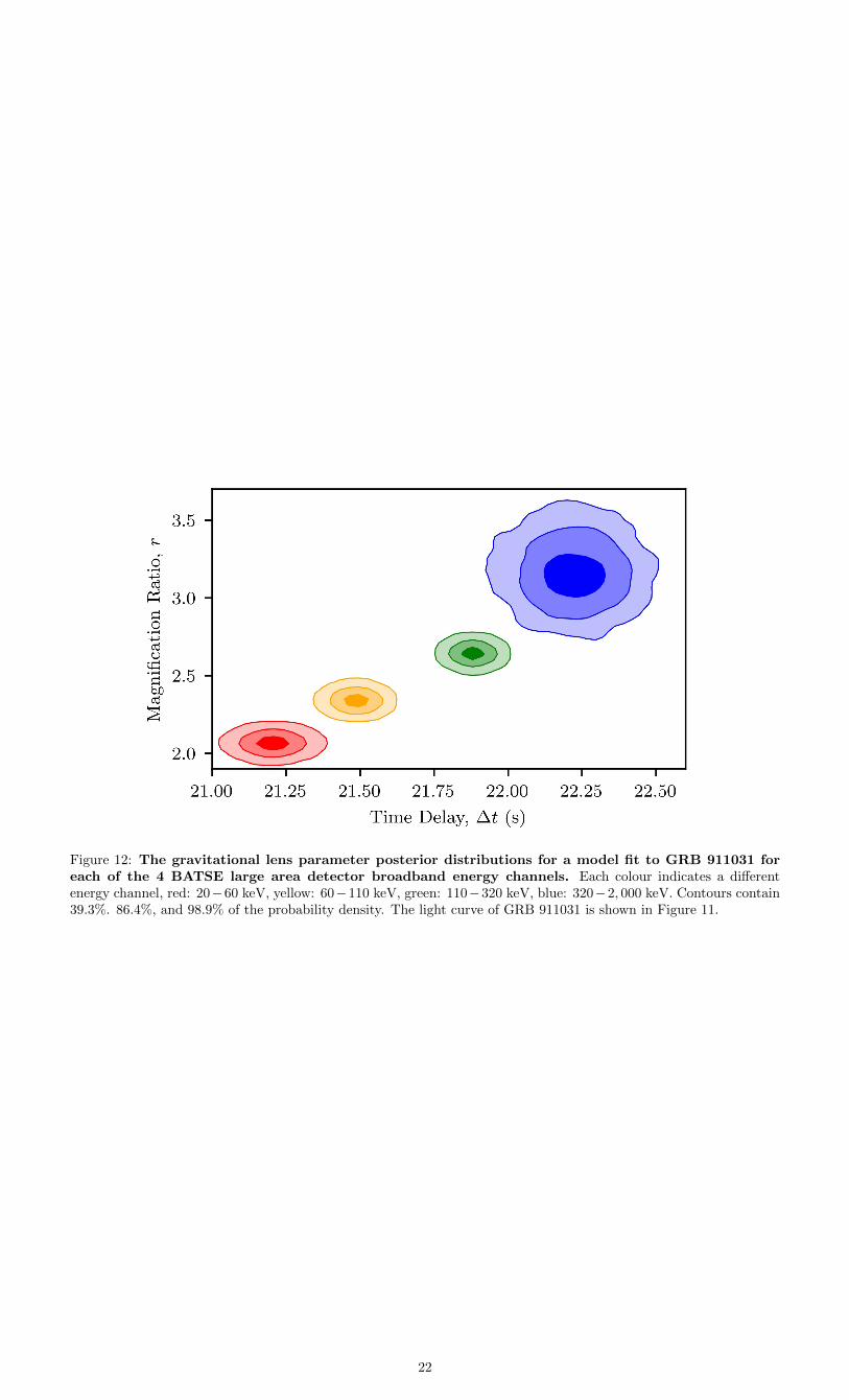
Figure 12: The gravitational lens parameter posterior distributions for a model fit to GRB 911031 foreach of the 4 BATSE large area detector broadband energy channels. Each colour indicates a differentenergy channel, red: 20−60 keV, yellow: 60−110 keV, green: 110−320 keV, blue: 320−2, 000 keV. Contours contain39.3%. 86.4%, and 98.9% of the probability density. The light curve of GRB 911031 is shown in Figure 11.

22