James J. Buckley Simulating Fuzzy Systems - … · Fuzzy probabilities and fuzzy parameters in...
208
James J. Buckley Simulating Fuzzy Systems
Transcript of James J. Buckley Simulating Fuzzy Systems - … · Fuzzy probabilities and fuzzy parameters in...

James J. Buckley
Simulating Fuzzy Systems

Studies in Fuzziness and Soft Computing, Volume 171
Editor-in-chiefProf. Janusz KacprzykSystems Research InstitutePolish Academy of Sciencesul. Newelska 601-447 WarsawPolandE-mail: [email protected]
Further volume of this seriescan be found on our homepage:springeronline.com
Vol. 157. R.A. Aliev, F. Fazlollahi, R.R. AlievSoft Computing and its Applications inBusiness and Economics, 2004ISBN 3-540-22138-7
Vol. 158. K.K. DompereCost-Benefit Analysis and the Theory ofFuzzy Decisions – Identification andMeasurement Theory, 2004ISBN 3-540-22154-9
Vol. 159. E. Damiani, L.C. Jain,M. Madravia (Eds.)Soft Computing in Software Engineering,2004ISBN 3-540-22030-5
Vol. 160. K.K. DompereCost-Benefit Analysis and the Theory ofFuzzy Decisions – Fuzzy Value Theory, 2004ISBN 3-540-22161-1
Vol. 161. N. Nedjah, L. de MacedoMourelle (Eds.)Evolvable Machines, 2005ISBN 3-540-22905-1
Vol. 162. R. Khosla, N. Ichalkaranje, L.C. JainDesign of Intelligent Multi-Agent Systems,2005ISBN 3-540-22913-2
Vol. 163. A. Ghosh, L.C. Jain (Eds.)Evolutionary Computation in Data Mining,2005ISBN 3-540-22370-3
Vol. 164. M. Nikravesh, L.A. Zadeh,J. Kacprzyk (Eds.)Soft Computing for Information Prodessingand Analysis, 2005ISBN 3-540-22930-2
Vol. 165. A.F. Rocha, E. Massad, A. Pereira Jr.The Brain: From Fuzzy Arithmetic toQuantum Computing, 2005ISBN 3-540-21858-0
Vol. 166. W.E. Hart, N. Krasnogor,J.E. Smith (Eds.)Recent Advances in Memetic Algorithms,2005ISBN 3-540-22904-3
Vol. 167. Y. Jin (Ed.)Knowledge Incorporation in EvolutionaryComputation, 2005ISBN 3-540-22902-7
Vol. 168. Yap P. Tan, Kim H. Yap,Lipo Wang (Eds.)Intelligent Multimedia Processing with SoftComputing, 2005ISBN 3-540-22902-7
Vol. 169. C.R. Bector, Suresh ChandraFuzzy Mathematical Programming andFuzzy Matrix Games, 2005ISBN 3-540-23729-1
Vol. 170. Martin PelikanHierarchical Bayesian OptimizationAlgorithm, 2005ISBN 3-540-23774-7
Vol. 171. James J. BuckleySimulating Fuzzy Systems, 2005ISBN 3-540-24116-7

James J. Buckley
Simulating Fuzzy Systems
123

Professor James J. BuckleyUniversity of Alabama at BirminghamDepartment of MathematicsBirmingham, AL 35294-1170USAE-mail: [email protected]
ISSN print edition: 1434-9922ISSN electronic edition: 1860-0808ISBN 3-540-24116-7 Springer Berlin Heidelberg New York
Library of Congress Control Number: 2004116660This work is subject to copyright. All rights are reserved, whether the whole or part of the materialis concerned, specifically the rights of translation, reprinting, reuse of illustrations, recitation,broadcasting, reproduction on microfilm or in any other way, and storage in data banks. Dupli-cation of this publication or parts thereof is permitted only under the provisions of the GermanCopyright Law of September 9, 1965, in its current version, and permission for use must always beobtained from Springer. Violations are liable for prosecution under the German Copyright Law.
Springer is a part of Springer Science+Business Mediaspringeronline.com
© Springer-Verlag Berlin Heidelberg 2005Printed in Germany
The use of general descriptive names, registered names, trademarks, etc. in this publication doesnot imply, even in the absence of a specific statement, that such names are exempt from the relevantprotective laws and regulations and therefore free for general use.
Typesetting: by the author and TechBooks using a Springer LATEX macro packageCover design: E. Kirchner, Springer HeidelbergPrinted on acid-free paper 62/3141/jl- 5 4 3 2 1 0

To Julianne and Helen

Contents
1 Introduction . . . . . . . . . . . . . . . . . . . . . . . . . . . . . . . . . . . . . . . . . . . . . . 11.1 Introduction . . . . . . . . . . . . . . . . . . . . . . . . . . . . . . . . . . . . . . . . . . . 11.2 Notation . . . . . . . . . . . . . . . . . . . . . . . . . . . . . . . . . . . . . . . . . . . . . . 31.3 Figures . . . . . . . . . . . . . . . . . . . . . . . . . . . . . . . . . . . . . . . . . . . . . . . . 3References . . . . . . . . . . . . . . . . . . . . . . . . . . . . . . . . . . . . . . . . . . . . . . . . . 4
2 Fuzzy Sets . . . . . . . . . . . . . . . . . . . . . . . . . . . . . . . . . . . . . . . . . . . . . . . . 52.1 Introduction . . . . . . . . . . . . . . . . . . . . . . . . . . . . . . . . . . . . . . . . . . . 52.2 Fuzzy Sets . . . . . . . . . . . . . . . . . . . . . . . . . . . . . . . . . . . . . . . . . . . . . 5
2.2.1 Fuzzy Numbers . . . . . . . . . . . . . . . . . . . . . . . . . . . . . . . . . . 52.2.2 Alpha-Cuts . . . . . . . . . . . . . . . . . . . . . . . . . . . . . . . . . . . . . . 72.2.3 Inequalities . . . . . . . . . . . . . . . . . . . . . . . . . . . . . . . . . . . . . . 82.2.4 Discrete Fuzzy Sets . . . . . . . . . . . . . . . . . . . . . . . . . . . . . . . 8
2.3 Fuzzy Arithmetic . . . . . . . . . . . . . . . . . . . . . . . . . . . . . . . . . . . . . . . 82.3.1 Extension Principle . . . . . . . . . . . . . . . . . . . . . . . . . . . . . . . 82.3.2 Interval Arithmetic . . . . . . . . . . . . . . . . . . . . . . . . . . . . . . . 92.3.3 Fuzzy Arithmetic . . . . . . . . . . . . . . . . . . . . . . . . . . . . . . . . . 10
2.4 Fuzzy Functions . . . . . . . . . . . . . . . . . . . . . . . . . . . . . . . . . . . . . . . . 112.4.1 Extension Principle . . . . . . . . . . . . . . . . . . . . . . . . . . . . . . . 112.4.2 Alpha-Cuts and Interval Arithmetic . . . . . . . . . . . . . . . . 122.4.3 Differences . . . . . . . . . . . . . . . . . . . . . . . . . . . . . . . . . . . . . . 13
2.5 Ordering/Ranking Fuzzy Numbers . . . . . . . . . . . . . . . . . . . . . . . . 142.6 Optimization . . . . . . . . . . . . . . . . . . . . . . . . . . . . . . . . . . . . . . . . . . 152.7 Discrete Versus Continuous . . . . . . . . . . . . . . . . . . . . . . . . . . . . . . 15References . . . . . . . . . . . . . . . . . . . . . . . . . . . . . . . . . . . . . . . . . . . . . . . . . 17
3 Fuzzy Estimation . . . . . . . . . . . . . . . . . . . . . . . . . . . . . . . . . . . . . . . . . 193.1 Introduction . . . . . . . . . . . . . . . . . . . . . . . . . . . . . . . . . . . . . . . . . . . 193.2 Fuzzy Probabilities . . . . . . . . . . . . . . . . . . . . . . . . . . . . . . . . . . . . . 193.3 Fuzzy Numbers from Confidence Intervals . . . . . . . . . . . . . . . . . 203.4 Fuzzy Arrival/Service Rates . . . . . . . . . . . . . . . . . . . . . . . . . . . . . 22
3.4.1 Fuzzy Arrival Rate . . . . . . . . . . . . . . . . . . . . . . . . . . . . . . . 223.4.2 Fuzzy Service Rate . . . . . . . . . . . . . . . . . . . . . . . . . . . . . . . 23
3.5 Fuzzy Probability Distributions . . . . . . . . . . . . . . . . . . . . . . . . . . 253.5.1 Fuzzy Binomial . . . . . . . . . . . . . . . . . . . . . . . . . . . . . . . . . . 25
VIII Contents
3.5.2 Fuzzy Estimator of µ in the Normal . . . . . . . . . . . . . . . . 273.5.3 Fuzzy Estimator of σ2 in the Normal . . . . . . . . . . . . . . . 283.5.4 Fuzzy Exponential . . . . . . . . . . . . . . . . . . . . . . . . . . . . . . . . 323.5.5 Fuzzy Uniform . . . . . . . . . . . . . . . . . . . . . . . . . . . . . . . . . . . 33
3.6 Summary . . . . . . . . . . . . . . . . . . . . . . . . . . . . . . . . . . . . . . . . . . . . . . 34References . . . . . . . . . . . . . . . . . . . . . . . . . . . . . . . . . . . . . . . . . . . . . . . . . 34
4 Fuzzy Probability Theory . . . . . . . . . . . . . . . . . . . . . . . . . . . . . . . . . 374.1 Introduction . . . . . . . . . . . . . . . . . . . . . . . . . . . . . . . . . . . . . . . . . . . 374.2 Fuzzy Binomial . . . . . . . . . . . . . . . . . . . . . . . . . . . . . . . . . . . . . . . . 374.3 Fuzzy Poisson . . . . . . . . . . . . . . . . . . . . . . . . . . . . . . . . . . . . . . . . . . 394.4 Fuzzy Normal . . . . . . . . . . . . . . . . . . . . . . . . . . . . . . . . . . . . . . . . . . 424.5 Fuzzy Exponential . . . . . . . . . . . . . . . . . . . . . . . . . . . . . . . . . . . . . . 444.6 Fuzzy Uniform . . . . . . . . . . . . . . . . . . . . . . . . . . . . . . . . . . . . . . . . . 46References . . . . . . . . . . . . . . . . . . . . . . . . . . . . . . . . . . . . . . . . . . . . . . . . . 48
5 Fuzzy Systems Theory . . . . . . . . . . . . . . . . . . . . . . . . . . . . . . . . . . . . 495.1 Introduction . . . . . . . . . . . . . . . . . . . . . . . . . . . . . . . . . . . . . . . . . . . 495.2 Fuzzy System . . . . . . . . . . . . . . . . . . . . . . . . . . . . . . . . . . . . . . . . . . 505.3 Computing Fuzzy Measures of Performance . . . . . . . . . . . . . . . . 51Reference . . . . . . . . . . . . . . . . . . . . . . . . . . . . . . . . . . . . . . . . . . . . . . . . . . 52
6 Simulation . . . . . . . . . . . . . . . . . . . . . . . . . . . . . . . . . . . . . . . . . . . . . . . . 53References . . . . . . . . . . . . . . . . . . . . . . . . . . . . . . . . . . . . . . . . . . . . . . . . . 55
7 Queuing I: One-Step Calculations . . . . . . . . . . . . . . . . . . . . . . . . . 577.1 Introduction . . . . . . . . . . . . . . . . . . . . . . . . . . . . . . . . . . . . . . . . . . . 577.2 One-Step Calculations . . . . . . . . . . . . . . . . . . . . . . . . . . . . . . . . . . 57
7.2.1 Fuzzy Calculations . . . . . . . . . . . . . . . . . . . . . . . . . . . . . . . 587.2.2 Simulation . . . . . . . . . . . . . . . . . . . . . . . . . . . . . . . . . . . . . . . 61
7.3 Multi-Step Calculations . . . . . . . . . . . . . . . . . . . . . . . . . . . . . . . . . 647.4 Rest of the Book . . . . . . . . . . . . . . . . . . . . . . . . . . . . . . . . . . . . . . . 66References . . . . . . . . . . . . . . . . . . . . . . . . . . . . . . . . . . . . . . . . . . . . . . . . . 67
8 Simulation Optimization . . . . . . . . . . . . . . . . . . . . . . . . . . . . . . . . . . 698.1 Introduction . . . . . . . . . . . . . . . . . . . . . . . . . . . . . . . . . . . . . . . . . . . 698.2 Arrivals . . . . . . . . . . . . . . . . . . . . . . . . . . . . . . . . . . . . . . . . . . . . . . . 698.3 Service . . . . . . . . . . . . . . . . . . . . . . . . . . . . . . . . . . . . . . . . . . . . . . . . 70
8.3.1 Exponential . . . . . . . . . . . . . . . . . . . . . . . . . . . . . . . . . . . . . 708.3.2 Uniform . . . . . . . . . . . . . . . . . . . . . . . . . . . . . . . . . . . . . . . . . 718.3.3 Normal . . . . . . . . . . . . . . . . . . . . . . . . . . . . . . . . . . . . . . . . . 72
8.4 Probabilistic Transfer . . . . . . . . . . . . . . . . . . . . . . . . . . . . . . . . . . . 738.5 Summary . . . . . . . . . . . . . . . . . . . . . . . . . . . . . . . . . . . . . . . . . . . . . . 73
Contents IX
9 Queuing II: No One-Step Calculations . . . . . . . . . . . . . . . . . . . . 759.1 Introduction . . . . . . . . . . . . . . . . . . . . . . . . . . . . . . . . . . . . . . . . . . . 759.2 Case 1: First Simulation . . . . . . . . . . . . . . . . . . . . . . . . . . . . . . . . . 759.3 Case 2: Second Simulation . . . . . . . . . . . . . . . . . . . . . . . . . . . . . . . 789.4 Case 3: Third Simulation . . . . . . . . . . . . . . . . . . . . . . . . . . . . . . . . 799.5 Summary . . . . . . . . . . . . . . . . . . . . . . . . . . . . . . . . . . . . . . . . . . . . . . 80Reference . . . . . . . . . . . . . . . . . . . . . . . . . . . . . . . . . . . . . . . . . . . . . . . . . . 80
10 Call Center Model . . . . . . . . . . . . . . . . . . . . . . . . . . . . . . . . . . . . . . . . 8110.1 Introduction . . . . . . . . . . . . . . . . . . . . . . . . . . . . . . . . . . . . . . . . . . . 8110.2 Case 1: First Simulation . . . . . . . . . . . . . . . . . . . . . . . . . . . . . . . . . 8210.3 Case 2: Second Simulation . . . . . . . . . . . . . . . . . . . . . . . . . . . . . . . 8310.4 Case 3: Third Simulation . . . . . . . . . . . . . . . . . . . . . . . . . . . . . . . . 8410.5 Summary . . . . . . . . . . . . . . . . . . . . . . . . . . . . . . . . . . . . . . . . . . . . . . 85Reference . . . . . . . . . . . . . . . . . . . . . . . . . . . . . . . . . . . . . . . . . . . . . . . . . . 85
11 Machine Shop I . . . . . . . . . . . . . . . . . . . . . . . . . . . . . . . . . . . . . . . . . . . 8711.1 Introduction . . . . . . . . . . . . . . . . . . . . . . . . . . . . . . . . . . . . . . . . . . . 8711.2 Case 1: First Simulation . . . . . . . . . . . . . . . . . . . . . . . . . . . . . . . . . 8911.3 Cases 2 and 3: Second and Third Simulation . . . . . . . . . . . . . . . 9111.4 Summary . . . . . . . . . . . . . . . . . . . . . . . . . . . . . . . . . . . . . . . . . . . . . . 92Reference . . . . . . . . . . . . . . . . . . . . . . . . . . . . . . . . . . . . . . . . . . . . . . . . . . 93
12 Machine Shop II . . . . . . . . . . . . . . . . . . . . . . . . . . . . . . . . . . . . . . . . . . 9512.1 Introduction . . . . . . . . . . . . . . . . . . . . . . . . . . . . . . . . . . . . . . . . . . . 9512.2 Case 1: First Simulation . . . . . . . . . . . . . . . . . . . . . . . . . . . . . . . . . 9712.3 Case 2: Second Simulation . . . . . . . . . . . . . . . . . . . . . . . . . . . . . . . 9812.4 Case 3: Third Simulation . . . . . . . . . . . . . . . . . . . . . . . . . . . . . . . . 10012.5 Summary . . . . . . . . . . . . . . . . . . . . . . . . . . . . . . . . . . . . . . . . . . . . . . 101Reference . . . . . . . . . . . . . . . . . . . . . . . . . . . . . . . . . . . . . . . . . . . . . . . . . . 101
13 Emergency Room Model . . . . . . . . . . . . . . . . . . . . . . . . . . . . . . . . . 10313.1 Introduction . . . . . . . . . . . . . . . . . . . . . . . . . . . . . . . . . . . . . . . . . . . 10313.2 Case 1: First Simulation . . . . . . . . . . . . . . . . . . . . . . . . . . . . . . . . . 10513.3 Case 2: Second Simulation . . . . . . . . . . . . . . . . . . . . . . . . . . . . . . . 10713.4 Case 3: Third Simulation . . . . . . . . . . . . . . . . . . . . . . . . . . . . . . . . 10813.5 Summary . . . . . . . . . . . . . . . . . . . . . . . . . . . . . . . . . . . . . . . . . . . . . . 108Reference . . . . . . . . . . . . . . . . . . . . . . . . . . . . . . . . . . . . . . . . . . . . . . . . . . 109
14 Machine Servicing Problem . . . . . . . . . . . . . . . . . . . . . . . . . . . . . . . 11114.1 Introduction . . . . . . . . . . . . . . . . . . . . . . . . . . . . . . . . . . . . . . . . . . . 11114.2 Case 1: First Simulation (k = 1) . . . . . . . . . . . . . . . . . . . . . . . . . . 11214.3 Case 2: Second Simulation (k = 2) . . . . . . . . . . . . . . . . . . . . . . . . 11414.4 Case 3: Third Simulation (k = 3) . . . . . . . . . . . . . . . . . . . . . . . . . 11514.5 Case 4: Fourth Simulation (k = 4) . . . . . . . . . . . . . . . . . . . . . . . . 115
X Contents
14.6 Case 5: Fifth Simulation (k = 5) . . . . . . . . . . . . . . . . . . . . . . . . . . 11514.7 Summary . . . . . . . . . . . . . . . . . . . . . . . . . . . . . . . . . . . . . . . . . . . . . . 115Reference . . . . . . . . . . . . . . . . . . . . . . . . . . . . . . . . . . . . . . . . . . . . . . . . . . 116
15 Life Insurance: New Account Model . . . . . . . . . . . . . . . . . . . . . . 11715.1 Introduction . . . . . . . . . . . . . . . . . . . . . . . . . . . . . . . . . . . . . . . . . . . 11715.2 Case 1: First Simulation . . . . . . . . . . . . . . . . . . . . . . . . . . . . . . . . . 11815.3 Case 2: Second Simulation . . . . . . . . . . . . . . . . . . . . . . . . . . . . . . . 12015.4 Case 3: Third Simulation . . . . . . . . . . . . . . . . . . . . . . . . . . . . . . . . 12115.5 Summary . . . . . . . . . . . . . . . . . . . . . . . . . . . . . . . . . . . . . . . . . . . . . . 121Reference . . . . . . . . . . . . . . . . . . . . . . . . . . . . . . . . . . . . . . . . . . . . . . . . . . 121
16 Inventory Control I . . . . . . . . . . . . . . . . . . . . . . . . . . . . . . . . . . . . . . . 12316.1 Introduction . . . . . . . . . . . . . . . . . . . . . . . . . . . . . . . . . . . . . . . . . . . 12316.2 Case 1: First Simulation . . . . . . . . . . . . . . . . . . . . . . . . . . . . . . . . . 12516.3 Case 2: Second Simulation . . . . . . . . . . . . . . . . . . . . . . . . . . . . . . . 12716.4 Case 3: Third Simulation . . . . . . . . . . . . . . . . . . . . . . . . . . . . . . . . 12816.5 Summary . . . . . . . . . . . . . . . . . . . . . . . . . . . . . . . . . . . . . . . . . . . . . . 129References . . . . . . . . . . . . . . . . . . . . . . . . . . . . . . . . . . . . . . . . . . . . . . . . . 129
17 Inventory Control II . . . . . . . . . . . . . . . . . . . . . . . . . . . . . . . . . . . . . . 13117.1 Introduction . . . . . . . . . . . . . . . . . . . . . . . . . . . . . . . . . . . . . . . . . . . 13117.2 Case 1: First Simulation . . . . . . . . . . . . . . . . . . . . . . . . . . . . . . . . . 13317.3 Case 2: Second Simulation . . . . . . . . . . . . . . . . . . . . . . . . . . . . . . . 13417.4 Case 3: Third Simulation . . . . . . . . . . . . . . . . . . . . . . . . . . . . . . . . 13517.5 Summary . . . . . . . . . . . . . . . . . . . . . . . . . . . . . . . . . . . . . . . . . . . . . . 136Reference . . . . . . . . . . . . . . . . . . . . . . . . . . . . . . . . . . . . . . . . . . . . . . . . . . 136
18 Oil Tanker Problem . . . . . . . . . . . . . . . . . . . . . . . . . . . . . . . . . . . . . . 13718.1 Introduction . . . . . . . . . . . . . . . . . . . . . . . . . . . . . . . . . . . . . . . . . . . 13718.2 Case 1: Super Tankers . . . . . . . . . . . . . . . . . . . . . . . . . . . . . . . . . . 13918.3 Case 2: Big Tankers . . . . . . . . . . . . . . . . . . . . . . . . . . . . . . . . . . . . 13918.4 Case 3: Regular Tankers . . . . . . . . . . . . . . . . . . . . . . . . . . . . . . . . . 14018.5 Summary . . . . . . . . . . . . . . . . . . . . . . . . . . . . . . . . . . . . . . . . . . . . . . 141References . . . . . . . . . . . . . . . . . . . . . . . . . . . . . . . . . . . . . . . . . . . . . . . . . 142
19 Priority Queues . . . . . . . . . . . . . . . . . . . . . . . . . . . . . . . . . . . . . . . . . . 14319.1 Introduction . . . . . . . . . . . . . . . . . . . . . . . . . . . . . . . . . . . . . . . . . . . 14319.2 Case 1: First Simulation . . . . . . . . . . . . . . . . . . . . . . . . . . . . . . . . . 14619.3 Case 2: Second Simulation . . . . . . . . . . . . . . . . . . . . . . . . . . . . . . . 14619.4 Case 3: Third Simulation . . . . . . . . . . . . . . . . . . . . . . . . . . . . . . . . 14719.5 Summary . . . . . . . . . . . . . . . . . . . . . . . . . . . . . . . . . . . . . . . . . . . . . . 148

Contents XI
20 Optimizing a Production Line . . . . . . . . . . . . . . . . . . . . . . . . . . . . 14920.1 Introduction . . . . . . . . . . . . . . . . . . . . . . . . . . . . . . . . . . . . . . . . . . . 14920.2 Simulations . . . . . . . . . . . . . . . . . . . . . . . . . . . . . . . . . . . . . . . . . . . . 15120.3 Summary . . . . . . . . . . . . . . . . . . . . . . . . . . . . . . . . . . . . . . . . . . . . . . 152Reference . . . . . . . . . . . . . . . . . . . . . . . . . . . . . . . . . . . . . . . . . . . . . . . . . . 154
21 Supermarket Model . . . . . . . . . . . . . . . . . . . . . . . . . . . . . . . . . . . . . . 15521.1 Introduction . . . . . . . . . . . . . . . . . . . . . . . . . . . . . . . . . . . . . . . . . . . 15521.2 Case 1: First Simulation . . . . . . . . . . . . . . . . . . . . . . . . . . . . . . . . . 15821.3 Case 2: Second Simulation . . . . . . . . . . . . . . . . . . . . . . . . . . . . . . . 15921.4 Case 3: Third Simulation . . . . . . . . . . . . . . . . . . . . . . . . . . . . . . . . 16021.5 Summary . . . . . . . . . . . . . . . . . . . . . . . . . . . . . . . . . . . . . . . . . . . . . . 160Reference . . . . . . . . . . . . . . . . . . . . . . . . . . . . . . . . . . . . . . . . . . . . . . . . . . 160
22 Bank Teller Problem . . . . . . . . . . . . . . . . . . . . . . . . . . . . . . . . . . . . . 16122.1 Introduction . . . . . . . . . . . . . . . . . . . . . . . . . . . . . . . . . . . . . . . . . . . 16122.2 First Simulation: Multiple Queues . . . . . . . . . . . . . . . . . . . . . . . . 16322.3 Second Simulation: Single Queue . . . . . . . . . . . . . . . . . . . . . . . . . 16322.4 Summary . . . . . . . . . . . . . . . . . . . . . . . . . . . . . . . . . . . . . . . . . . . . . . 163References . . . . . . . . . . . . . . . . . . . . . . . . . . . . . . . . . . . . . . . . . . . . . . . . . 164
23 A Bus Stop . . . . . . . . . . . . . . . . . . . . . . . . . . . . . . . . . . . . . . . . . . . . . . . 16523.1 Introduction . . . . . . . . . . . . . . . . . . . . . . . . . . . . . . . . . . . . . . . . . . . 16523.2 Case 1: First Simulation . . . . . . . . . . . . . . . . . . . . . . . . . . . . . . . . . 16623.3 Case 2: More Buses . . . . . . . . . . . . . . . . . . . . . . . . . . . . . . . . . . . . . 16723.4 Case 3: Larger Buses . . . . . . . . . . . . . . . . . . . . . . . . . . . . . . . . . . . . 16823.5 Summary . . . . . . . . . . . . . . . . . . . . . . . . . . . . . . . . . . . . . . . . . . . . . . 168Reference . . . . . . . . . . . . . . . . . . . . . . . . . . . . . . . . . . . . . . . . . . . . . . . . . . 168
24 Process Failure/Spare Parts Problem . . . . . . . . . . . . . . . . . . . . . 16924.1 Introduction . . . . . . . . . . . . . . . . . . . . . . . . . . . . . . . . . . . . . . . . . . . 16924.2 Case 1: No Spare Parts . . . . . . . . . . . . . . . . . . . . . . . . . . . . . . . . . . 17124.3 Case 2: One Spare Part . . . . . . . . . . . . . . . . . . . . . . . . . . . . . . . . . 17124.4 Case 3: Two Spare Parts . . . . . . . . . . . . . . . . . . . . . . . . . . . . . . . . 17124.5 Case 4: Three Spare Parts . . . . . . . . . . . . . . . . . . . . . . . . . . . . . . . 17224.6 Summary . . . . . . . . . . . . . . . . . . . . . . . . . . . . . . . . . . . . . . . . . . . . . . 172Reference . . . . . . . . . . . . . . . . . . . . . . . . . . . . . . . . . . . . . . . . . . . . . . . . . . 173
25 Preemptive Service . . . . . . . . . . . . . . . . . . . . . . . . . . . . . . . . . . . . . . . 17525.1 Introduction . . . . . . . . . . . . . . . . . . . . . . . . . . . . . . . . . . . . . . . . . . . 17525.2 Case 1: First Simulation . . . . . . . . . . . . . . . . . . . . . . . . . . . . . . . . . 17725.3 Case 2: Second Simulation . . . . . . . . . . . . . . . . . . . . . . . . . . . . . . . 17725.4 Case 3: Third Simulation . . . . . . . . . . . . . . . . . . . . . . . . . . . . . . . . 17925.5 Summary . . . . . . . . . . . . . . . . . . . . . . . . . . . . . . . . . . . . . . . . . . . . . . 179Reference . . . . . . . . . . . . . . . . . . . . . . . . . . . . . . . . . . . . . . . . . . . . . . . . . . 179

XII Contents
26 Project Network Model . . . . . . . . . . . . . . . . . . . . . . . . . . . . . . . . . . . 18126.1 Introduction . . . . . . . . . . . . . . . . . . . . . . . . . . . . . . . . . . . . . . . . . . . 18126.2 Simulations . . . . . . . . . . . . . . . . . . . . . . . . . . . . . . . . . . . . . . . . . . . . 18326.3 Maximize Profit . . . . . . . . . . . . . . . . . . . . . . . . . . . . . . . . . . . . . . . . 18526.4 Summary . . . . . . . . . . . . . . . . . . . . . . . . . . . . . . . . . . . . . . . . . . . . . . 186References . . . . . . . . . . . . . . . . . . . . . . . . . . . . . . . . . . . . . . . . . . . . . . . . . 186
27 Summary and Conclusions . . . . . . . . . . . . . . . . . . . . . . . . . . . . . . . . 187References . . . . . . . . . . . . . . . . . . . . . . . . . . . . . . . . . . . . . . . . . . . . . . . . . 188
28 Simulation Programs . . . . . . . . . . . . . . . . . . . . . . . . . . . . . . . . . . . . . 18928.1 Introduction . . . . . . . . . . . . . . . . . . . . . . . . . . . . . . . . . . . . . . . . . . 18928.2 Chapter 9 . . . . . . . . . . . . . . . . . . . . . . . . . . . . . . . . . . . . . . . . . . . . . 18928.3 Chapter 10 . . . . . . . . . . . . . . . . . . . . . . . . . . . . . . . . . . . . . . . . . . . . 19128.4 Chapter 11 . . . . . . . . . . . . . . . . . . . . . . . . . . . . . . . . . . . . . . . . . . . . 19228.5 Chapter 12 . . . . . . . . . . . . . . . . . . . . . . . . . . . . . . . . . . . . . . . . . . . . 19228.6 Chapter 13 . . . . . . . . . . . . . . . . . . . . . . . . . . . . . . . . . . . . . . . . . . . . 19528.7 Chapter 17 . . . . . . . . . . . . . . . . . . . . . . . . . . . . . . . . . . . . . . . . . . . . 19628.8 Chapter 18 . . . . . . . . . . . . . . . . . . . . . . . . . . . . . . . . . . . . . . . . . . . . 20028.9 Chapter 22 . . . . . . . . . . . . . . . . . . . . . . . . . . . . . . . . . . . . . . . . . . . . 20128.10 Chapter 25 . . . . . . . . . . . . . . . . . . . . . . . . . . . . . . . . . . . . . . . . . . . . 20228.11 Chapter 26 . . . . . . . . . . . . . . . . . . . . . . . . . . . . . . . . . . . . . . . . . . . . 203
Index . . . . . . . . . . . . . . . . . . . . . . . . . . . . . . . . . . . . . . . . . . . . . . . . . . . . . . . . . 205

1 Introduction
1.1 Introduction
This book is written in two major parts. The first part includes the introduc-tory chapters consisting of Chaps. 1 through 8. In part two, Chaps. 9–26, wepresent the applications.
First we need to be familiar with fuzzy sets. All you need to know aboutfuzzy sets for this book comprises Chap. 2. For a beginning introduction tofuzzy sets and fuzzy logic see [6].
Chapter 3 gives a brief introduction to fuzzy estimation. We explain howyou can get fuzzy numbers when you estimate, from crisp data, probabilitiesor parameters in probability densities. The basic construction involves placingconfidence intervals, one on top of another, to obtain a fuzzy number as ourestimator instead of using a point estimator or a single confidence interval.
Fuzzy probabilities and fuzzy parameters in probability densities givesrise to fuzzy distributions. In Chap. 4 we look more closely at the fuzzy bi-nomial, fuzzy Poisson, fuzzy normal, fuzzy exponential and the fuzzy uniformdistribution. These are the fuzzy distributions that we will be using in therest of the book. For all of these fuzzy distributions we want to see how theyare used to compute fuzzy probabilities.
Chapter 5 introduces fuzzy systems theory. Consider any system whosedescription employs probability theory. Assume that some of these proba-bilities must be estimated from crisp data, and/or some the parameters inthe probability densities must be estimated from crisp data. Using our fuzzyestimators (Chap. 3) we obtain fuzzy probabilities and fuzzy distributions.Now we want to compute certain system descriptors like R = the expectedtime it takes an item to pass through the system and N = the expectednumber of items in the system. The fuzziness in the probabilities and proba-bility densities propagates through the system producing fuzzy numbers forR and N . We have a fuzzy system. A main problem with fuzzy systems [2, 9]is: how will we accomplish all the needed fuzzy calculations to compute thesystem descriptors? This is the main topic of this book: use crisp simulationto estimate the fuzzy numbers describing system performance.
How do we choose simulation software to accomplish all the simulationsin Chaps. 7, 9–26 is the topic of Chap. 6. We discuss cost, ease of use, need to
James J. Buckley: Simulating Fuzzy Systems, StudFuzz 171, 1–4 (2005)www.springerlink.com c© Springer-Verlag Berlin Heidelberg 2005

2 1 Introduction
run on a desktop computer, must compile system statistics we are interestedin, plus some others. Our final decision is also discussed.
Simulation can not be used to approximate all fuzzy calculations. Whichfuzzy computations can be approximated is the topic of Chap. 7. Considera very simple queuing system where customers arrive and possibly enter aqueue waiting for service in a single server and after service they depart thesystem. If the server is vacant the customer can go directly into the server.We want to find N = the expected number of customers in the system.The input to the model is λ = the arrival rate and µ = the service rate.In any operations research book we may find a function f to compute N interms of λ and µ, or N = f(λ, µ). Assume that λ and µ must be estimatedfrom data on the system. We obtain fuzzy estimators which incorporate theuncertainty in the data. So now λ and µ become fuzzy numbers. Put the fuzzynumbers into the function f and determine, using the extension principle(Chap. 2), the fuzzy number for N . We argue in Chap. 7 that simulationcan estimate alpha-cuts (horizontal slices, Chap. 2) of N . We say that N canbe gotten in a one-step calculation since we have N a function of λ and µ.Next consider finding N using a two-step calculation. Here we first find thesteady-state probabilities from the λ and µ and then get N as a function ofthe steady-state probabilities. Then λ and µ become fuzzy, the steady-stateprobabilities are fuzzy and finally we get fuzzy N . In this case N is obtainedas the result of a two-step calculation. We argue in Chap. 7 that simulationmay not approximate horizontal cuts of fuzzy N from a two-step (or more)calculation.
Chapter 8 introduces a type of simulation optimization. We discuss howwe plan to solve the simulation optimization problems presented in (5.4) and(5.5) of Chap. 5, and (7.20) and (7.21) of Chap. 7. This solution must beperformed in all Chaps. 9–26.
The structure of the rest of the book is now determined. Use simulationto approximate fuzzy system descriptors in fuzzy systems where the fuzzynumber to be approximated can be assumed to be the result of a one-stepcalculation but the system is sufficiently complicated so that we do not knowthis one-step function. This will be the topic of Chaps. 9–26.
The applications in Chaps. 9–26 are quite varied ranging from emergencyrooms to machine shops to project scheduling showing the varieties of fuzzysystems. These chapters may be read independently (except Chaps. 11,12and 16,17 go together). This means some material, including discussion ofsteady-state, fuzzy estimators, one-step functions, etc., are repeated in eachchapter.
Selected simulation programs are in Chap. 28. These simulation programs,including minimal comments, are listed in that chapter. We could not includeall the programs because that would make the Chap. 40 pages long, too muchdevoted to computer programs in a book around 200 pages. A reader may
1.3 Figures 3
obtain other simulation programs by contacting the author via email withtheir requests.
This book is based on, but expanded from, the following recent papersand publications: (1) fuzzy estimation, probability and statistics [1, 2, 3, 4],[7,8, 9]; (2) fuzzy systems [5]; and (3) simulating fuzzy systems [10, 11].
There are no prerequisites, but it would be helpful to know some basicinformation about queuing systems. However, the reader should be able tounderstand, from the figures and analytical development, how simulation isuseful in analyzing fuzzy systems.
1.2 Notation
It is difficult, in a book with a lot of mathematics, to achieve a uniformnotation without having to introduce many new specialized symbols. Ourbasic notation is presented in Chap. 2. What we have done is to have auniform notation within each chapter. What this means is that we may usethe letters “a” and “b” to represent a closed interval [a, b] in one chapter butthey could stand for parameters in a probability density in another chapter.We will have the following uniform notation throughout the book: (1) weplace a “bar” over a letter to denote a fuzzy set (A, B, etc.), and all ourfuzzy sets will be fuzzy subsets of the real numbers; and (2) an alpha-cut ofa fuzzy set (Chap. 2) is always denoted by “α”. Since we will be using α foralpha-cuts we need to change some standard notation in statistics: we use βin confidence intervals. So a (1 − β)100% confidence interval means a 95%confidence interval if β = 0.05. When a confidence interval switches to beingan alpha-cut of a fuzzy number (see Chap. 3), we switch from β to α. Allfuzzy arithmetic is performed using the extension principle (Chap. 2). Theterm “crisp” means not fuzzy. A crisp set is a regular set and a crisp numberis a real number. Also, throughout the book x will be the mean of a randomsample, not a fuzzy set.
1.3 Figures
Some of the figures, graphs of certain fuzzy numbers, in the book are difficultto obtain so they were created using different methods. Many graphs weredone first in Maple [12] and then exported to LaTeX2ε. We did these figuresfirst in Maple because of the “implicitplot” command in Maple. Let us ex-plain why this command was important in this book. Suppose X is a fuzzyestimator we want to graph. Usually in this book we determine X by firstcalculating its α-cuts. Let X[α] = [x1(α), x2(α)]. So we get x = x1(α) de-scribing the left side of the triangular shaped fuzzy number X and x = x2(α)describes the right side. On a graph we would have the x-axis horizontal andthe y-axis vertical. α is on the y-axis between zero and one. Substituting y

4 1 Introduction
for α we need to graph x = xi(y), for i = 1, 2. But this is backwards, weusually have y a function of x. The “implicitplot” command allows us to dothe correct graph with x a function of y when we have x = xi(y). Figures2.1–2.3, 3.1–3.7, 4.1, 4.3, and 4.5 were done in Maple and then exported toLaTeX2ε. All the other figures were constructed in LaTeX2ε.
References
1. J.J. Buckley: Fuzzy Probabilities: New Approach and Applications,Physica-Verlag, Heidelberg, Germany, 2003. 3
2. J.J. Buckley: Fuzzy Probabilities and Fuzzy Sets for Web Planning, Springer,Heidelberg, Germany, 2004. 1, 3
3. J.J. Buckley: Fuzzy Statistics, Springer, Heidelberg, Germany, 2004. 34. J.J. Buckley: Uncertain Probabilities III: The Continuous Case, Soft Comput-
ing, 8(2004)200-206. 35. J.J. Buckley: Fuzzy Systems, Soft Computing. To appear. 36. J.J. Buckley and E. Eslami: An Introduction to Fuzzy Logic and Fuzzy Sets,
Physica-Verlag, Heidelberg, Germany, 2002. 17. J.J. Buckley and E. Eslami: Uncertain Probabilities I: The Discrete Case, Soft
Computing, 7(2003)500-505. 38. J.J. Buckley and E. Eslami: Uncertain Probabilities II: The Continuous Case,
Soft Computing, 8(2004)193-199. 39. J.J. Buckley, K. Reilly and X. Zheng: Fuzzy Probabilities for Web Planning,
Soft Computing, 8(2004)464-476. 1, 310. J.J. Buckley, K. Reilly and X. Zheng: Simulating Fuzzy Systems I, in:
Applied Research in Uncertainty Modelling and Analysis, Eds. N.O. Attoh-Okine, B. Ayyub, Kluwer, 2004. To appear. 3
11. J.J. Buckley, K. Reilly and X. Zheng: Simulating Fuzzy Systems II, in: AppliedResearch in Uncertainty Modelling and Analysis, Eds. N.O. Attoh-Okine, B.Ayyub, Kluwer, 2004. To appear. 3
12. Maple 9, Waterloo Maple Inc., Waterloo, Canada. 3

2 Fuzzy Sets
2.1 Introduction
In this chapter we have collected together the basic ideas from fuzzy setsand fuzzy functions needed for the book. Any reader familiar with fuzzy sets,fuzzy numbers, the extension principle, α-cuts, interval arithmetic, and fuzzyfunctions may go on and have a look at Sects. 2.5, 2.6 and 2.7. In Sect. 2.5we discuss the method we will be using in this book to evaluate comparisonsbetween fuzzy numbers. That is, in Sect. 2.5 we need to decide which oneof the following three possibilities is true: M < N ; M ≈ N ; or M > N , forfuzzy numbers M and N . In Sect. 2.6, using Sect. 2.5, we solve, for smallsets of fuzzy numbers, maxM i and minM i, 1 ≤ i ≤ n. Section 2.6 explainshow, and why, we will approximate discrete fuzzy sets with fuzzy numbers.A good general reference for fuzzy sets and fuzzy logic is [4] and [8].
Our notation specifying a fuzzy set is to place a “bar” over a letter. SoX, M , T , . . . , µ, p, σ2, a, b, . . . , all denote fuzzy sets.
2.2 Fuzzy Sets
If Ω is some set, then a fuzzy subset A of Ω is defined by its membershipfunction, written A(x), which produces values in [0, 1] for all x in Ω. So, A(x)is a function mapping Ω into [0, 1]. If A(x0) = 1, then we say x0 belongs toA, if A(x1) = 0 we say x1 does not belong to A, and if A(x2) = 0.6 we saythe membership value of x2 in A is 0.6. When A(x) is always equal to oneor zero we obtain a crisp (non-fuzzy) subset of Ω. For all fuzzy sets B, C, . . .we use B(x), C(x), . . . for the value of their membership function at x. Thefuzzy sets we will be using will be fuzzy numbers .
The term “crisp” will mean not fuzzy. A crisp set is a regular set. Acrisp number is just a real number. A crisp function maps real numbers (orreal vectors) into real numbers. A crisp solution to a problem is a solutioninvolving crisp sets, crisp numbers, crisp functions, etc.
2.2.1 Fuzzy Numbers
A general definition of fuzzy number may be found in [4, 8], however ourfuzzy numbers will be triangular (shaped) fuzzy numbers. A triangular fuzzy
James J. Buckley: Simulating Fuzzy Systems, StudFuzz 171, 5–18 (2005)www.springerlink.com c© Springer-Verlag Berlin Heidelberg 2005

6 2 Fuzzy Sets
0
0.2
0.4
0.6
0.8
1
alpha
0.5 1 1.5 2 2.5 3x
Fig. 2.1. Triangular Fuzzy Number N
number N is defined by three numbers a < b < c where the base of thetriangle is the interval [a, c] and its vertex is at x = b. Triangular fuzzynumbers will be written as N = (a/b/c). A triangular fuzzy number N =(1.2/2/2.4) is shown in Fig. 2.1. We see that N(2) = 1, N(1.6) = 0.5, etc.
A triangular shaped fuzzy number P is given in Fig. 2.2. P is only partiallyspecified by the three numbers 1.2, 2, 2.4 since the graph on [1.2, 2], and[2, 2.4], is not a straight line segment. To be a triangular shaped fuzzy numberwe require the graph to be continuous and: (1) monotonically increasing on
0
0.2
0.4
0.6
0.8
1
alpha
0.5 1 1.5 2 2.5 3x
Fig. 2.2. Triangular Shaped Fuzzy Number P

2.2 Fuzzy Sets 7
[1.2, 2]; and (2) monotonically decreasing on [2, 2.4]. For triangular shapedfuzzy number P we use the notation P ≈ (1.2/2/2.4) to show that it ispartially defined by the three numbers 1.2, 2, and 2.4. If P ≈ (1.2/2/2.4) weknow its base is on the interval [1.2, 2.4] with vertex (membership value one)at x = 2.
2.2.2 Alpha-Cuts
Alpha-cuts are slices through a fuzzy set producing regular (non-fuzzy) sets.If A is a fuzzy subset of some set Ω, then an α-cut of A, written A[α], isdefined as
A[α] = x ∈ Ω|A(x) ≥ α , (2.1)
for all α, 0 < α ≤ 1. The α = 0 cut, or A[0], must be defined separately.Let N be the fuzzy number in Fig. 2.1. Then N [0] = [1.2, 2.4]. Notice that
using (2.1) to define N [0] would give N [0] = all the real numbers. Similarly,in Fig. 2.2 P [0] = [1.2, 2.4]. For any fuzzy set A, A[0] is called the support, orbase, of A. Many authors call the support of a fuzzy number the open interval(a, b) like the support of N in Fig. 2.1 would then be (1.2, 2.4). However inthis book we use the closed interval [a, b] for the support (base) of the fuzzynumber.
The core of a fuzzy number is the set of values where the membershipvalue equals one. If N = (a/b/c), or N ≈ (a/b/c), then the core of N is thesingle point b.
For any fuzzy number Q we know that Q[α] is a closed, bounded, intervalfor 0 ≤ α ≤ 1. We will write this as
Q[α] = [q1(α), q2(α)] , (2.2)
where q1(α) (q2(α)) will be an increasing (decreasing) function of α withq1(1) = q2(1). If Q is a triangular shaped then: (1) q1(α) will be a continuous,monotonically increasing function of α in [0, 1]; (2) q2(α) will be a continuous,monotonically decreasing function of α, 0 ≤ α ≤ 1; and (3) q1(1) = q2(1) .
For the N in Fig. 2.1 we obtain N [α] = [n1(α), n2(α)], n1(α) = 1.2 + 0.8αand n2(α) = 2.4−0.4α, 0 ≤ α ≤ 1. The equation for ni(α) is backwards. Withthe y-axis vertical and the x-axis horizontal the equation n1(α) = 1.2 + 0.8αmeans x = 1.2 + 0.8y, 0 ≤ y ≤ 1. That is, the straight line segment from(1.2, 0) to (2, 1) in Fig. 2.1 is given as x a function of y whereas it is usuallystated as y a function of x. This is how it will be done for all α-cuts of fuzzynumbers.
The general requirements for a fuzzy set N of the real numbers to be afuzzy number are: (1) it must be normalized, or N(x) = 1 for some x; and (2)its alpha-cuts must be closed, bounded, intervals for all alpha in [0, 1]. Thiswill be important in fuzzy estimation because there the fuzzy numbers willhave very short vertical line segments at both ends of its base (see Sect. 3.3in Chap. 3). Even so, such a fuzzy set still meets the general requirementspresented above to be called a fuzzy number.

8 2 Fuzzy Sets
2.2.3 Inequalities
Let N = (a/b/c). We write N ≥ δ, δ some real number, if a ≥ δ, N > δ whena > δ, N ≤ δ for c ≤ δ and N < δ if c < δ. We use the same notation fortriangular shaped fuzzy numbers whose support is the interval [a, c].
If A and B are two fuzzy subsets of a set Ω, then A ≤ B means A(x) ≤B(x) for all x in Ω, or A is a fuzzy subset of B. A < B holds when A(x) <B(x), for all x. There is a potential problem with the symbol <. In someplaces in the book, for example see Sect. 2.5, M < N for fuzzy numbers Mand N means that M is less than N . It should be clear on how we use “<”as to which meaning is correct.
2.2.4 Discrete Fuzzy Sets
Let A be a fuzzy subset of Ω. If A(x) is not zero only at a finite number ofx values in Ω, then A is called a discrete fuzzy set. Suppose A(x) is not zeroonly at x1, x2, x3 and x4 in Ω. Then we write the fuzzy set as
A =
µ1
x1, . . . ,
µ4
x4
, (2.3)
where the µi are the membership values. That is, A(xi) = µi, 1 ≤ i ≤ 4,and A(x) = 0 otherwise. We can have discrete fuzzy subsets of any space Ω.Notice that α-cuts of discrete fuzzy sets of IR, the set of real numbers, do notproduce closed, bounded, intervals.
2.3 Fuzzy Arithmetic
If A and B are two fuzzy numbers we will need to add, subtract, multiply anddivide them. There are two basic methods of computing A + B, A − B, etc.which are: (1) extension principle; and (2) α-cuts and interval arithmetic.
2.3.1 Extension Principle
Let A and B be two fuzzy numbers. If A + B = C, then the membershipfunction for C is defined as
C(z) = supx,y
min(A(x), B(y))|x + y = z . (2.4)
If we set C = A − B, then
C(z) = supx,y
min(A(x), B(y))|x − y = z . (2.5)
Similarly, C = A · B, then

2.3 Fuzzy Arithmetic 9
C(z) = supx,y
min(A(x), B(y))|x · y = z , (2.6)
and if C = A/B,
C(z) = supx,y
min(A(x), B(y))|x/y = z . (2.7)
In all cases C is also a fuzzy number [8]. We assume that zero does not belongto the support of B in C = A/B. If A and B are triangular (shaped) fuzzynumbers then so are A+B and A−B, but A ·B and A/B will be triangularshaped fuzzy numbers.
We should mention something about the operator “sup” in (2.3)–(2.6). IfΩ is a set of real numbers bounded above (there is a M so that x ≤ M , forall x in Ω), then sup(Ω) = the least upper bound for Ω. If Ω has a maximummember, then sup(Ω) = max(Ω). For example, if Ω = [0, 1), sup(Ω) = 1 butif Ω = [0, 1], then sup(Ω) = max(Ω) = 1. The dual operator to “sup” is “inf”.If Ω is bounded below (there is a M so that M ≤ x for all x ∈ Ω), theninf(Ω) = the greatest lower bound. For example, for Ω = (0, 1] inf(Ω) = 0but if Ω = [0, 1], then inf(Ω) = min(Ω) = 0.
Obviously, given A and B, (2.3)–(2.6) appear quite complicated to com-pute A+B, A−B, etc. So, we now present another procedure based on α-cutsand interval arithmetic. First, we present the basics of interval arithmetic.
2.3.2 Interval Arithmetic
We only give a brief introduction to interval arithmetic. For more informationthe reader is referred to [9, 10]. Let [a1, b1] and [a2, b2] be two closed, bounded,intervals of real numbers. If ∗ denotes addition, subtraction, multiplication,or division, then [a1, b1] ∗ [a2, b2] = [α, β] where
[α, β] = a ∗ b|a1 ≤ a ≤ b1, a2 ≤ b ≤ b2 . (2.8)
If ∗ is division, we must assume that zero does not belong to [a2, b2]. We maysimplify (2.8) as follows:
[a1, b1] + [a2, b2] = [a1 + a2, b1 + b2] , (2.9)[a1, b1] − [a2, b2] = [a1 − b2, b1 − a2] , (2.10)
[a1, b1] / [a2, b2] = [a1, b1] ·[
1b2
,1a2
], (2.11)
and[a1, b1] · [a2, b2] = [α, β] , (2.12)
where
α = mina1a2, a1b2, b1a2, b1b2 , (2.13)β = maxa1a2, a1b2, b1a2, b1b2 . (2.14)

10 2 Fuzzy Sets
Multiplication and division may be further simplified if we know thata1 > 0 and b2 < 0, or b1 > 0 and b2 < 0, etc. For example, if a1 ≥ 0 anda2 ≥ 0, then
[a1, b1] · [a2, b2] = [a1a2, b1b2] , (2.15)
and if b1 < 0 but a2 ≥ 0, we see that
[a1, b1] · [a2, b2] = [a1b2, a2b1] . (2.16)
Also, assuming b1 < 0 and b2 < 0 we get
[a1, b1] · [a2, b2] = [b1b2, a1a2] , (2.17)
but a1 ≥ 0, b2 < 0 produces
[a1, b1] · [a2, b2] = [a2b1, b2a1] . (2.18)
2.3.3 Fuzzy Arithmetic
Again we have two fuzzy numbers A and B. We know α-cuts are closed,bounded, intervals so let A[α] = [a1(α), a2(α)], B[α] = [b1(α), b2(α)]. Then ifC = A + B we have
C[α] = A[α] + B[α] . (2.19)
We add the intervals using (2.8). Setting C = A − B we get
C[α] = A[α] − B[α] , (2.20)
for all α in [0, 1]. AlsoC[α] = A[α] · B[α] , (2.21)
for C = A · B andC[α] = A[α]/B[α] , (2.22)
when C = A/B, provided that zero does not belong to B[α] for all α. Thismethod is equivalent to the extension principle method of fuzzy arithmetic[8]. Obviously, this procedure, of α-cuts plus interval arithmetic, is more user(and computer) friendly.
Example 2.3.3.1
Let A = (−3/ − 2/ − 1) and B = (4/5/6). We determine A · B using α-cutsand interval arithmetic. We compute A[α] = [−3 + α,−1 − α] and B[α] =[4 + α, 6−α]. So, if C = A·B we obtain C[α] = [(α−3)(6−α), (−1−α)(4 + α)],0 ≤ α ≤ 1. The graph of C is shown in Fig. 2.3.

2.4 Fuzzy Functions 11
0
0.2
0.4
0.6
0.8
1
alpha
–18 –16 –14 –12 –10 –8 –6 –4x
Fig. 2.3. The Fuzzy Number C = A · B
2.4 Fuzzy Functions
In this book a fuzzy function is a mapping from fuzzy numbers into fuzzynumbers. We write H(X) = Z for a fuzzy function with one independentvariable X. X will be a triangular (shaped) fuzzy number and then we usuallyobtain Z as a triangular (shaped) shaped fuzzy number. For two independentvariables we have H(X,Y ) = Z.
Where do these fuzzy functions come from? They are usually extensions ofreal-valued functions. Let h : [a, b] → IR. This notation means z = h(x) for xin [a, b] and z a real number. One extends h : [a, b] → IR to H(X) = Z in twoways: (1) the extension principle; or (2) using α-cuts and interval arithmetic.
2.4.1 Extension Principle
Any h : [a, b] → IR may be extended to H(X) = Z as follows
Z(z) = supx
X(x)|h(x) = z, a ≤ x ≤ b
. (2.23)
Equation (2.22) defines the membership function of Z for any triangular(shaped) fuzzy number X in [a, b].
If h is continuous, then we have a way to find α-cuts of Z. Let Z[α] =[z1(α), z2(α)]. Then [5]
z1(α) = minh(x)|x ∈ X[α] , (2.24)z2(α) = maxh(x)|x ∈ X[α] , (2.25)
for 0 ≤ α ≤ 1.

12 2 Fuzzy Sets
If we have two independent variables, then let z = h(x, y) for x in [a1, b1],y in [a2, b2]. We extend h to H(X,Y ) = Z as
Z(z) = supx,y
min
(X(x), Y (y)
)|h(x, y) = z
, (2.26)
for X (Y ) a triangular (shaped) fuzzy number in [a1, b1] ([a2, b2]). For α-cutsof Z, assuming h is continuous, we have
z1(α) = minh(x, y)|x ∈ X[α], y ∈ Y [α] , (2.27)z2(α) = maxh(x, y)|x ∈ X[α], y ∈ Y [α] , (2.28)
0 ≤ α ≤ 1.
2.4.2 Alpha-Cuts and Interval Arithmetic
All the functions we usually use in engineering and science have a computeralgorithm which, using a finite number of additions, subtractions, multiplica-tions and divisions, can evaluate the function to required accuracy [5]. Suchfunctions can be extended, using α-cuts and interval arithmetic, to fuzzy func-tions. Let h : [a, b] → IR be such a function. Then its extension H(X) = Z, Xin [a, b] is done, via interval arithmetic, in computing h(X[α]) = Z[α], α in[0, 1]. We input the interval X[α], perform the arithmetic operations neededto evaluate h on this interval, and obtain the interval Z[α]. Then put theseα-cuts together to obtain the value Z. The extension to more independentvariables is straightforward.
For example, consider the fuzzy function
Z = H(X) =A X + B
C X + D, (2.29)
for triangular fuzzy numbers A, B, C, D and triangular fuzzy number X in[0, 10]. We assume that C ≥ 0, D > 0 so that C X + D > 0. This would bethe extension of
h(x1, x2, x3, x4, x) =x1x + x2
x3x + x4. (2.30)
We would substitute the intervals A[α] for x1, B[α] for x2, C[α] for x3, D[α]for x4 and X[α] for x, do interval arithmetic, to obtain interval Z[α] for Z.Alternatively, the fuzzy function
Z = H(X) =2X + 103X + 4
, (2.31)
would be the extension of
h(x) =2x + 103x + 4
. (2.32)
2.4 Fuzzy Functions 13
2.4.3 Differences
Let h : [a, b] → IR. Just for this subsection let us write Z∗= H(X) for the
extension principle method of extending h to H for X in [a, b]. We denoteZ = H(X) for the α-cut and interval arithmetic extension of h .
We know that Z can be different from Z∗. But for basic fuzzy arithmetic
in Sect. 2.3 the two methods give the same results. In the example belowwe show that for h(x) = x(1 − x), x in [0, 1], we can get Z
∗ = Z for someX in [0, 1]. What is known ([5],[9]) is that for usual functions in science andengineering Z
∗ ≤ Z. Otherwise, there is no known necessary and sufficientconditions on h so that Z
∗= Z for all X in [a, b].
There is nothing wrong in using α-cuts and interval arithmetic to evaluatefuzzy functions. Surely, it is user, and computer friendly. However, we shouldbe aware that whenever we use α-cuts plus interval arithmetic to computeZ = H(X) we may be getting something larger than that obtained fromthe extension principle. The same results hold for functions of two or moreindependent variables.
Example 2.4.3.1
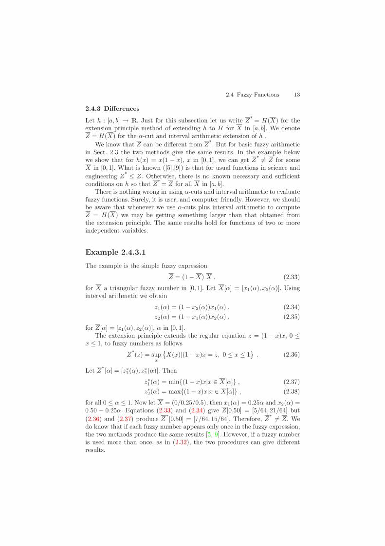
The example is the simple fuzzy expression
Z = (1 − X) X , (2.33)
for X a triangular fuzzy number in [0, 1]. Let X[α] = [x1(α), x2(α)]. Usinginterval arithmetic we obtain
z1(α) = (1 − x2(α))x1(α) , (2.34)z2(α) = (1 − x1(α))x2(α) , (2.35)
for Z[α] = [z1(α), z2(α)], α in [0, 1].The extension principle extends the regular equation z = (1 − x)x, 0 ≤
x ≤ 1, to fuzzy numbers as follows
Z∗(z) = sup
x
X(x)|(1 − x)x = z, 0 ≤ x ≤ 1
. (2.36)
Let Z∗[α] = [z∗1(α), z∗2(α)]. Then
z∗1(α) = min(1 − x)x|x ∈ X[α] , (2.37)z∗2(α) = max(1 − x)x|x ∈ X[α] , (2.38)
for all 0 ≤ α ≤ 1. Now let X = (0/0.25/0.5), then x1(α) = 0.25α and x2(α) =0.50 − 0.25α. Equations (2.33) and (2.34) give Z[0.50] = [5/64, 21/64] but(2.36) and (2.37) produce Z
∗[0.50] = [7/64, 15/64]. Therefore, Z
∗ = Z. Wedo know that if each fuzzy number appears only once in the fuzzy expression,the two methods produce the same results [5, 9]. However, if a fuzzy numberis used more than once, as in (2.32), the two procedures can give differentresults.

14 2 Fuzzy Sets
2.5 Ordering/Ranking Fuzzy Numbers
This section is about ordering/ranking a finite set of fuzzy numbers. Givena finite set of fuzzy numbers A1, . . . , An, we want to order/rank them fromsmallest to largest. For a finite set of real numbers there is no problem inordering them from smallest to largest. However, in the fuzzy case thereis no universally accepted way to do this. There are probably more than40 methods proposed in the literature of defining M ≤ N , for two fuzzynumbers M and N . Here the symbol ≤ means “less than or equal” and not“a fuzzy subset of”. A few key references on this topic are [1, 6, 7, 11, 12],where the interested reader can look up many of these methods and see theircomparisons.
Here we will present only one procedure for ordering fuzzy numbers thatwe have used before [2, 3]. But note that different definitions of ≤ betweenfuzzy numbers can give different ordering. We first define ≤ between twofuzzy numbers M and N . Define
v(M ≤ N) = maxmin(M(x), N(y))|x ≤ y , (2.39)
which measures how much M is less than or equal to N . We write N < Mif v(N ≤ M) = 1 but v(M ≤ N) < η, where η is some fixed fraction in(0, 1]. In this book we will use η = 0.8. Then N < M if v(N ≤ M) = 1 andv(M ≤ N) < 0.8. We then define M ≈ N when both N < M and M < N arefalse. M ≤ N means M < N or M ≈ N . Now this ≈ may not be transitive.If N ≈ M and M ≈ O implies that N ≈ O, then ≈ is transitive. However, itcan happen that N ≈ M and M ≈ O but N < O because M lies a little tothe right of N and O lies a little to the right of M but O lies sufficiently farto the right of N that we obtain N < O. But this ordering is still useful inpartitioning the set of fuzzy numbers up into sets H1, . . . , HK where [2, 3]:(1) given any M and N in Hk, 1 ≤ k ≤ K, then M ≈ N ; and (2) givenN ∈ Hi and M ∈ Hj , with i < j, then N ≤ M . Then the highest rankedfuzzy numbers lie in HK , the second highest ranked fuzzy numbers are inHK−1, etc. This result is easily seen if you graph all the fuzzy numbers onthe same axis then those in HK will be clustered together farthest to theright, proceeding from the HK cluster to the left the next cluster will bethose in HK−1, etc.
There is an easy way to determine if M < N , or M ≈ N , for manyfuzzy numbers. First, it is easy to see that if the core of N lies completely tothe right of the core of M , then v(M ≤ N) = 1. Also, if the core of M and thecore of N overlap, then M ≈ N . Now assume that the core of N lies to theright of the core of M , as shown in Fig. 2.4 for triangular fuzzy numbers,and we wish to compute v(N ≤ M). The value of this expression is simplyy0 in Fig. 2.4. In general, for triangular (shaped) fuzzy numbers v(N ≤ M)is the height of their intersection when the core of N lies to the right ofthe core of M . Locate η, for example η = 0.8 in this book, on the vertical

2.7 Discrete Versus Continuous 15
0 1 2 3 4 5x
1
y
MN
(x0, y0)
Fig. 2.4. Determining M < N
axis and then draw a horizontal line through η. If in Fig. 2.4 y0 lies belowthe horizontal line, then M < N . If y0 lies on, or above, the horizontal line,then M ≈ N .
2.6 Optimization
Given a finite set of fuzzy numbers M i, 1 ≤ i ≤ n, we will sometimes, inChaps. 9–26, want to find maxM i and/or minM i. We will use the graphicalmethod from Sect. 2.5. This works well when the set of fuzzy numbers issmall but becomes “messy”, or too cluttered, when the set of fuzzy numbersis large.
First consider the fuzzy numbers M i, i = 1, 2, 3, shown in Fig. 2.5 and wewant maxM i. Clearly, using η = 0.8 from Sect. 2.5, we get M2 < M3 < M1
and maxM i = M1.Next consider the fuzzy numbers M i, 1 ≤ i ≤ 6, in Fig. 2.6 and we
want minM i. Using η = 0.8 we have M1 ≈ M6 < M i, i = 2, 3, 4, 5. HenceminM i = M1,M6.
2.7 Discrete Versus Continuous
In Chaps. 7 and 9 through 26 there are a number of fuzzy sets we willwant to determine and they may be discrete fuzzy sets or fuzzy numbers(now also called continuous fuzzy sets). Examples of discrete fuzzy sets maybe: (1) LC = number of lost customers per unit time; (2) MQ = maxi-mum queue length for a certain queue in the fuzzy system; (3) N = ex-pected (mean) number of transactions (customers, items) in the fuzzy system;
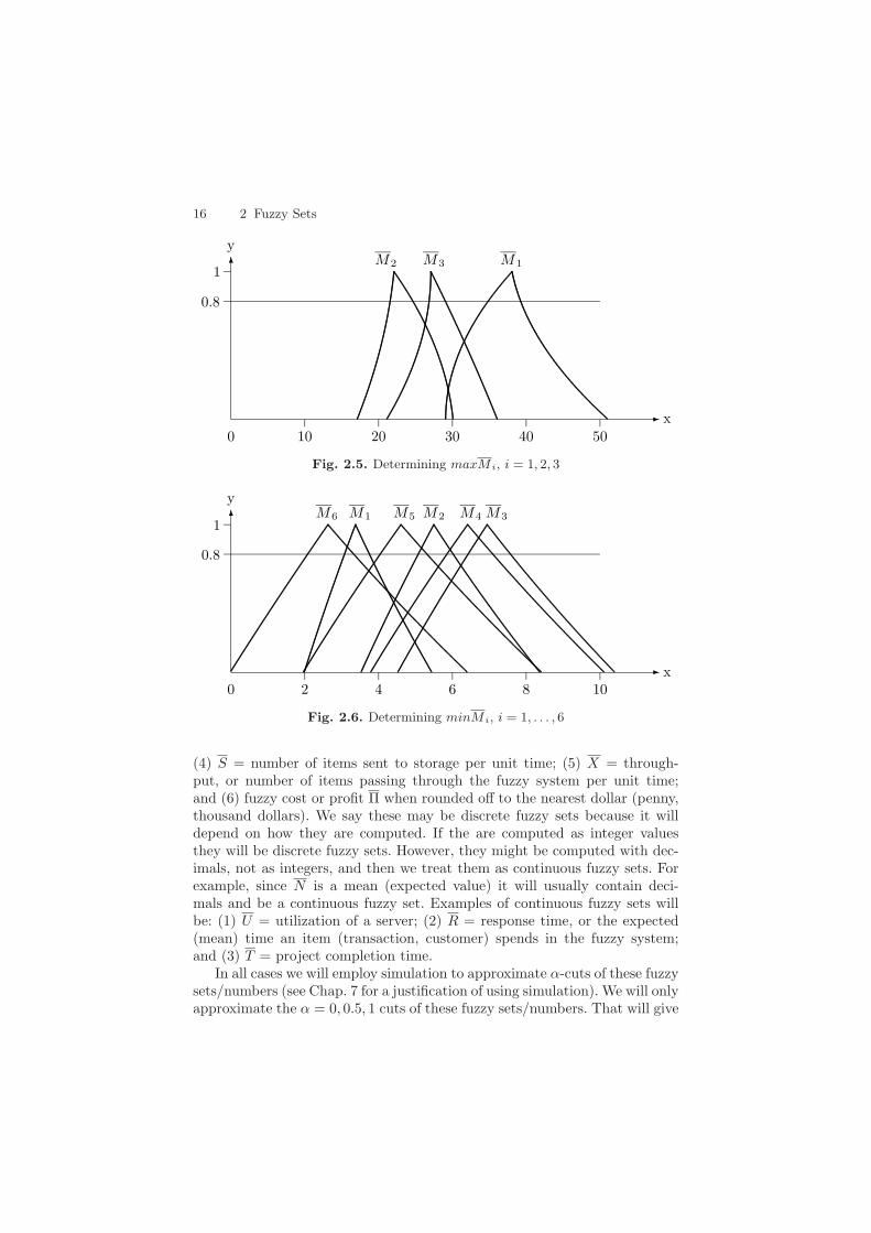
16 2 Fuzzy Sets
0.8
0 10 20 30 40 50x
1
yM1M2 M3
Fig. 2.5. Determining maxM i, i = 1, 2, 3
0.8
0 2 4 6 8 10x
1
yM3M2M6 M5M1 M4
Fig. 2.6. Determining minM i, i = 1, . . . , 6
(4) S = number of items sent to storage per unit time; (5) X = through-put, or number of items passing through the fuzzy system per unit time;and (6) fuzzy cost or profit Π when rounded off to the nearest dollar (penny,thousand dollars). We say these may be discrete fuzzy sets because it willdepend on how they are computed. If the are computed as integer valuesthey will be discrete fuzzy sets. However, they might be computed with dec-imals, not as integers, and then we treat them as continuous fuzzy sets. Forexample, since N is a mean (expected value) it will usually contain deci-mals and be a continuous fuzzy set. Examples of continuous fuzzy sets willbe: (1) U = utilization of a server; (2) R = response time, or the expected(mean) time an item (transaction, customer) spends in the fuzzy system;and (3) T = project completion time.
In all cases we will employ simulation to approximate α-cuts of these fuzzysets/numbers (see Chap. 7 for a justification of using simulation). We will onlyapproximate the α = 0, 0.5, 1 cuts of these fuzzy sets/numbers. That will give

References 17
0 24 48 72 96 120x
1
y
Fig. 2.7. Discrete Fuzzy Set MQ
us only five points to approximate the graphs of these fuzzy sets/numbers. Foran example consider approximating MQ. Let MQ[0] = [26, 121], MQ[0.5] =[45, 100] and MQ[1] = 70. Then we have the following five points in the graphof the membership function: (26, 0), (45, 0.5), (70, 1), (100, 0.5), (121, 0). Forall the discrete fuzzy sets we will now draw a continuous curve through thethree points on the left side, and draw a continuous curve through the threepoints on the right side, producing a graph of a continuous fuzzy set. Thismakes the discrete fuzzy set appear to be a fuzzy number. See Fig. 2.7. Thefive points are plotted as small dark circles within the approximating fuzzynumber.
Why did we do this to discrete fuzzy sets? This makes all our graphsuniform so the fuzzy sets may be compared using Sects. 2.5 and 2.6. Also,constructing graphs through three points is very easy using the graphingcommand “qbezier” in LaTeX. We will try to remind the reader about thisapproximating a discrete fuzzy set by a fuzzy number whenever it occurs inthe rest of the book.
References
1. G. Bortolon and R. Degani: A Review of Some Methods for Ranking FuzzySubsets, Fuzzy Sets and Systems, 15(1985)1-19. 14
2. J.J. Buckley: Ranking Alternatives Using Fuzzy Numbers, Fuzzy Sets and Sys-tems, 15(1985)21-31. 14
3. J.J. Buckley: Fuzzy Hierarchical Analysis, Fuzzy Sets and Systems, 17(1985)233-247. 14
4. J.J. Buckley and E. Eslami: Introduction to Fuzzy Logic and Fuzzy Sets,Physica-Verlag, Heidelberg, Germany, 2002. 5
18 2 Fuzzy Sets
5. J.J. Buckley and Y. Qu: On Using α-Cuts to Evaluate Fuzzy Equations, FuzzySets and Systems, 38(1990)309-312. 12, 13
6. P.T. Chang and E.S. Lee: Fuzzy Arithmetic and Comparison of Fuzzy Numbers,in: Fuzzy Optimization: Recent Advances, Eds. M. Delgado, J. Kacprzyk, J.L.Verdegay and M.A. Vila, Physica-Verlag, Heidelberg, Germany, 1994, 69-81. 14
7. D. Dubois, E. Kerre, R. Mesiar and H. Prade: Fuzzy Interval Analysis, in:Fundamentals of Fuzzy Sets, The Handbook of Fuzzy Sets, Eds. D. Dubois andH. Prade, Kluwer Acad. Publ., 2000, 483-581. 14
8. G.J. Klir and B. Yuan: Fuzzy Sets and Fuzzy Logic: Theory and Applications,Prentice Hall, Upper Saddle River, N.J., 1995. 5, 9, 10
9. R.E. Moore: Methods and Applications of Interval Analysis, SIAM Studies inApplied Mathematics, Philadelphia, 1979. 9, 13
10. A. Neumaier: Interval Methods for Systems of Equations, Cambridge UniversityPress, Cambridge, U.K., 1990. 9
11. X. Wang and E.E. Kerre: Reasonable Properties for the Ordering of FuzzyQuantities (I), Fuzzy Sets and Systems, 118(2001)375-385. 14
12. X. Wang and E.E. Kerre: Reasonable Properties for the Ordering of FuzzyQuantities (II), Fuzzy Sets and Systems, 118(2001)387-405. 14

3 Fuzzy Estimation
3.1 Introduction
The first thing to do is explain how we will get fuzzy numbers , and fuzzyprobabilities, from a set of confidence intervals which will be constructedfrom crisp data. This is done in the next two sections. Next we discuss howwe can obtain fuzzy numbers for arrival rates and for service rates in queuingsystems. Then we discuss the fuzzy binomial, the fuzzy normal, the fuzzyexponential and the fuzzy uniform distributions. These will be the fuzzyprobability distributions used in the rest of the book. The material in thischapter has been adapted from results in references [1, 7].
3.2 Fuzzy Probabilities
Let X = x1, . . . , xn be a finite set and let P be a probability functiondefined on all subsets of X with P (xi) = ai, 1 ≤ i ≤ n, 0 < ai < 1, all i,and
∑ni=1 ai = 1. We may substitute a fuzzy number ai for ai, for some i,
to obtain a discrete (finite) fuzzy probability distribution . Where do thesefuzzy numbers come from?
In some problems, because of the way the problem is stated, the valuesof all the ai are crisp and known. For example, consider tossing a fair coinand a1 = the probability of getting a “head” and a2 = is the probabilityof obtaining a “tail”. Since we assumed it to be a fair coin we must havea1 = a2 = 0.5. In this case we would not substitute a fuzzy number for a1 ora2. But in many other problems the ai are not known exactly and they areeither estimated from a random sample or they are obtained from “expertopinion”.
Suppose we have the results of a random sample to estimate the value ofa1. We would construct a set of confidence intervals for a1 and then put thesetogether to get the fuzzy number a1 for a1. This method of building a fuzzynumber from confidence intervals is discussed in detail in the next section.
Assume that we do not know the values of the ai and we do not haveany data to estimate their values. Then we may obtain numbers for the ai
from some group of experts. This group could consist of only one expert. Thiscase includes subjective, or “personal”, probabilities. First assume we have
James J. Buckley: Simulating Fuzzy Systems, StudFuzz 171, 19–35 (2005)www.springerlink.com c© Springer-Verlag Berlin Heidelberg 2005

20 3 Fuzzy Estimation
only one expert and he is to estimate the value of some probability p. Wecan solicit this estimate from the expert as is done in estimating job timesin project scheduling ([11], Chap. 13). Let a = the “pessimistic” value of p,or the smallest possible value, let c = be the “optimistic” value of p, or thehighest possible value, and let b = the most likely value of p. We then ask theexpert to give values for a, b, c and we construct the triangular fuzzy numberp = (a/b/c) for p. If we have a group of N experts all to estimate the valueof p we solicit the ai, bi and ci, 1 ≤ i ≤ N , from them. Let a be the averageof the ai, b is the mean of the bi and c is the average of the ci. The simplestthing to do is to use (a/b/c) for p.
3.3 Fuzzy Numbers from Confidence Intervals
We will be using fuzzy numbers for parameters in probability density func-tions (probability mass functions, the discrete case) and in this section weshow how we obtain these fuzzy numbers from a set of confidence intervals.Let X be a random variable with probability density function (or proba-bility mass function) f(x; θ) for single parameter θ. It is easy to generalizeour method to the case where θ is a vector of parameters. Assume that θis unknown and it must be estimated from a random sample X1, . . . , Xn.Let Y = u(X1, . . . , Xn) be a statistic used to estimate θ. Given the valuesof these random variables Xi = xi, 1 ≤ i ≤ n, we obtain a point estimateθ∗ = y = u(x1, . . . , xn) for θ. We would never expect this point estimate toexactly equal θ so we often also compute a (1 − β)100% confidence intervalfor θ. We are using β here since α, usually employed for confidence interval, isreserved for α-cuts of fuzzy numbers. In this confidence interval one usuallysets β equal to 0.10, 0.05 or 0.01.
We propose to find the (1−β)100% confidence interval for all 0.01≤β < 1.Starting at 0.01 is arbitrary and you could begin at 0.001 or 0.005 etc. Denotethese confidence intervals as
[θ1(β), θ2(β)] , (3.1)
for 0.01 ≤ β < 1. Add to this the interval [θ∗, θ∗] for the 0% confidenceinterval for θ. Then we have (1− β)100% confidence interval for θ for 0.01 ≤β ≤ 1.
Now place these confidence intervals, one on top of the other, to produce atriangular shaped fuzzy number θ whose α-cuts are the confidence intervals.We have
θ[α] = [θ1(α), θ2(α)] , (3.2)
for 0.01 ≤ α ≤ 1. All that is needed is to finish the “bottom” of θ to make ita complete fuzzy number. We will simply drop the graph of θ straight downto complete its α-cuts so

3.3 Fuzzy Numbers from Confidence Intervals 21
θ[α] = [θ1(0.01), θ2(0.01)] , (3.3)
for 0 ≤ α < 0.01. In this way we are using more information in θ than just apoint estimate, or just a single interval estimate.
The following example shows that the fuzzy mean of the normal probabil-ity density will be a triangular shaped fuzzy number. However, for simplicity,throughout this book we will always use triangular fuzzy numbers for thefuzzy values of uncertain parameters in probability density (mass) functions.
Example 3.3.1
Consider X a random variable with probability density function N(µ, 100),which is the normal probability density with unknown mean µ and knownvariance σ2 = 100. To estimate µ we obtain a random sample X1, . . . , Xn
from N(µ, 100). Suppose the mean of this random sample turns out to be28.6. Then a (1 − β)100% confidence interval for µ is
[θ1(β), θ2(β)] = [28.6 − zβ/210/√
n, 28.6 + zβ/210/√
n] , (3.4)
where zβ/2 is defined as∫ zβ/2
−∞N(0, 1)dx = 1 − β/2 , (3.5)
and N(0, 1) denotes the normal density with mean zero and unit variance.To obtain a graph of fuzzy µ, or µ, let n = 64. Then we evaluated (3.4) and(3.5) using Maple [9] and the final graph of µ is shown in Fig. 3.1, withoutdropping the graph straight down to the x-axis at the end points.
0
0.2
0.4
0.6
0.8
1
alpha
26 27 28 29 30 31x
Fig. 3.1. Fuzzy Mean µ in Example 3.3.1

22 3 Fuzzy Estimation
In future chapters we will have fuzzy numbers for the parameters inthe probability density (mass) functions producing fuzzy probability den-sity (mass) functions. These fuzzy probability density (mass) functions arediscussed in the next chapter.
3.4 Fuzzy Arrival/Service Rates
In this section we concentrate on deriving fuzzy numbers for the arrival rate,and the service rate, in a queuing system. We consider the fuzzy arrival ratefirst.
3.4.1 Fuzzy Arrival Rate
We assume that we have Poisson arrivals ([11], Chap. 15) which means thatthere is a positive constant λ so that the probability of k arrivals per unittime is
λk exp(−λ)/k! , (3.6)
the Poisson probability function. We need to estimate λ, the arrival rate, sowe take a random sample X1, . . . , Xm of size m. In the random sample Xi
is the number of arrivals per unit time, in the ith observation. Let S be thesum of the Xi and let X be S/m. Here, X is not a fuzzy set but the mean.
Now S is Poisson with parameter mλ ([8], p. 298). Assuming that mλis sufficiently large (say, at least 30), we may use the normal approximation([8], p. 317), so the statistic
W =S − mλ√
mλ, (3.7)
is approximately a standard normal. Then
P [−zβ/2 < W < zβ/2] = 1 − β , (3.8)
where the zβ/2 was defined in (3.5). Now divide numerator and denominatorof W by m and we get
P [−zβ/2 < Z < zβ/2] = 1 − β , (3.9)
where
Z =X − λ√
λ/m. (3.10)
From these last two equations we may derive an approximate (1 − β)100%confidence interval for λ. Let us call this confidence interval [l(β), r(β)].
We now show how to compute l(β) and r(β). Let

3.4 Fuzzy Arrival/Service Rates 23
f(λ) =√
m(X − λ)/√
λ . (3.11)
Now f(λ) has the following properties: (1) it is strictly decreasing for λ > 0;(2) it is zero for λ > 0 only at X = λ; (3) the limit of f , as λ goes to ∞ is−∞; and (4) the limit of f as λ approaches zero from the right is ∞. Hence,(1) the equation zβ/2 = f(λ) has a unique solution λ = l(β); and (2) theequation −zβ/2 = f(λ) also has a unique solution λ = r(β).
We may find these unique solutions. Let
V =√
z2β/2/m + 4X , (3.12)
z1 =[−
zβ/2√m
+ V
] /2 , (3.13)
and
z2 =[zβ/2√
m+ V
]/2 . (3.14)
Then l(β) = z21 and r(β) = z2
2 .We now substitute α for β to get the α-cuts of fuzzy number λ. Add the
point estimate, when α = 1, X, for the 0% confidence interval. Now as αgoes from 0.01 (99% confidence interval) to one (0% confidence interval) weget the fuzzy number for λ. As before, we drop the graph straight down atthe ends to obtain a complete fuzzy number.
Example 3.4.1.1
Suppose m = 100 and we obtained X = 25. We evaluated (3.12) through(3.14) using Maple [9] and then the graph of λ is shown in Fig. 3.2, withoutdropping the graph straight down to the x-axis at the end points. However,in the rest of the book we will use a triangular fuzzy number for λ.
3.4.2 Fuzzy Service Rate
Let µ be the average (expected) service rate, in the number of service com-pletions per unit time, for a busy server. Then 1/µ is the average (expected)service time. The probability density of the time interval between successiveservice completions is ([11], Chap. 15)
(1/µ) exp(−t/µ) , (3.15)
for t > 0, the exponential probability density function. Let X1, . . . , Xn be arandom sample from this exponential density function. Then the maximumlikelihood estimator for µ is X ([8], p. 344), the mean of the random sample(not a fuzzy set). We know that the probability density for X is the gamma

24 3 Fuzzy Estimation
0
0.2
0.4
0.6
0.8
1
alpha
24 24.5 25 25.5 26x
Fig. 3.2. Fuzzy Arrival Rate λ in Example 3.4.1.1
([8], p. 297) with mean µ and variance µ2/n ([8], p. 351). If n is sufficientlylarge we may use the normal approximation to determine approximate con-fidence intervals for µ. Let
Z = (√
n[X − µ])/µ , (3.16)
which is approximately normally distributed with zero mean and unit vari-ance, provided n is sufficiently large. See Fig. 3.2 in [8] for n = 100 whichshows the approximation is quite good if n = 100. The graph in Fig. 3.2 in [8]is for the chi-square distribution which is a special case of the gamma distri-bution. So we now assume that n ≥ 100 and use the normal approximationto the gamma.
An approximate (1 − β)100% confidence interval for µ is obtained from
P [−zβ/2 < Z < zβ/2] = 1 − β , (3.17)
where β was defined in (3.5). After solving for µ we get
P [L(β) < µ < R(β)] = 1 − β , (3.18)
whereL(β) = [
√n X]/[zβ/2 +
√n] , (3.19)
andR(β) = [
√n X]/[
√n − zβ/2] . (3.20)
An approximate (1 − β)100% confidence interval for µ is[ √
n X
zβ/2 +√
n,
√n X√
n − zβ/2
]. (3.21)
3.5 Fuzzy Probability Distributions 25
0.2
0.4
0.6
0.8
1
alpha
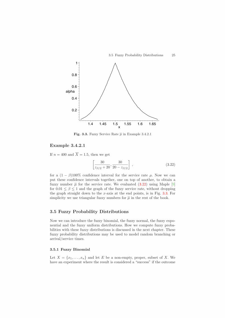
1.4 1.45 1.5 1.55 1.6 1.65x
Fig. 3.3. Fuzzy Service Rate µ in Example 3.4.2.1
Example 3.4.2.1
If n = 400 and X = 1.5, then we get[
30zβ/2 + 20
,30
20 − zβ/2
], (3.22)
for a (1 − β)100% confidence interval for the service rate µ. Now we canput these confidence intervals together, one on top of another, to obtain afuzzy number µ for the service rate. We evaluated (3.22) using Maple [9]for 0.01 ≤ β ≤ 1 and the graph of the fuzzy service rate, without droppingthe graph straight down to the x-axis at the end points, is in Fig. 3.3. Forsimplicity we use triangular fuzzy numbers for µ in the rest of the book.
3.5 Fuzzy Probability Distributions
Now we can introduce the fuzzy binomial, the fuzzy normal, the fuzzy expo-nential and the fuzzy uniform distributions. How we compute fuzzy proba-bilities with these fuzzy distributions is discussed in the next chapter. Thesefuzzy probability distributions may be used to model random branching orarrival/service times.
3.5.1 Fuzzy Binomial
Let X = x1, . . . , xn and let E be a non-empty, proper, subset of X. Wehave an experiment where the result is considered a “success” if the outcome
26 3 Fuzzy Estimation
xi is in E. Otherwise, the result is considered a “failure”. Let P (E) = p sothat P (E′) = q = 1 − p. P (E) is the probability of success and P (E′) is theprobability of failure. We assume that 0 < p < 1. Let X be a random variablewhich is one if the outcome is a success and zero when it is a failure. Theprobability mass function of X is
f(x) = px(1 − p)1−x , (3.23)
for x = 0, 1. We say that X has a Bernoulli distribution. If p is not knownprecisely it must be estimated. We could obtain a fuzzy estimator p for pthrough expert opinion or from data as discussed below for the binomialdistribution. Using fuzzy p we get the fuzzy Bernoulli distribution. The fuzzyBernoulli will be used to model random branching where p could be theprobability of an item being defective.
Suppose we have m independent repetitions of this experiment discussedabove. If P (r) is the probability of r successes in the m experiments, then
P (r) =(
m
r
)prqm−r , (3.24)
for r = 0, 1, 2, . . . ,m, gives the binomial distribution.In these experiments let us assume that P (E) = p is not known precisely
and it needs to be estimated from data, or obtained from expert opinion. Letus assume that we estimate p from some crisp data.
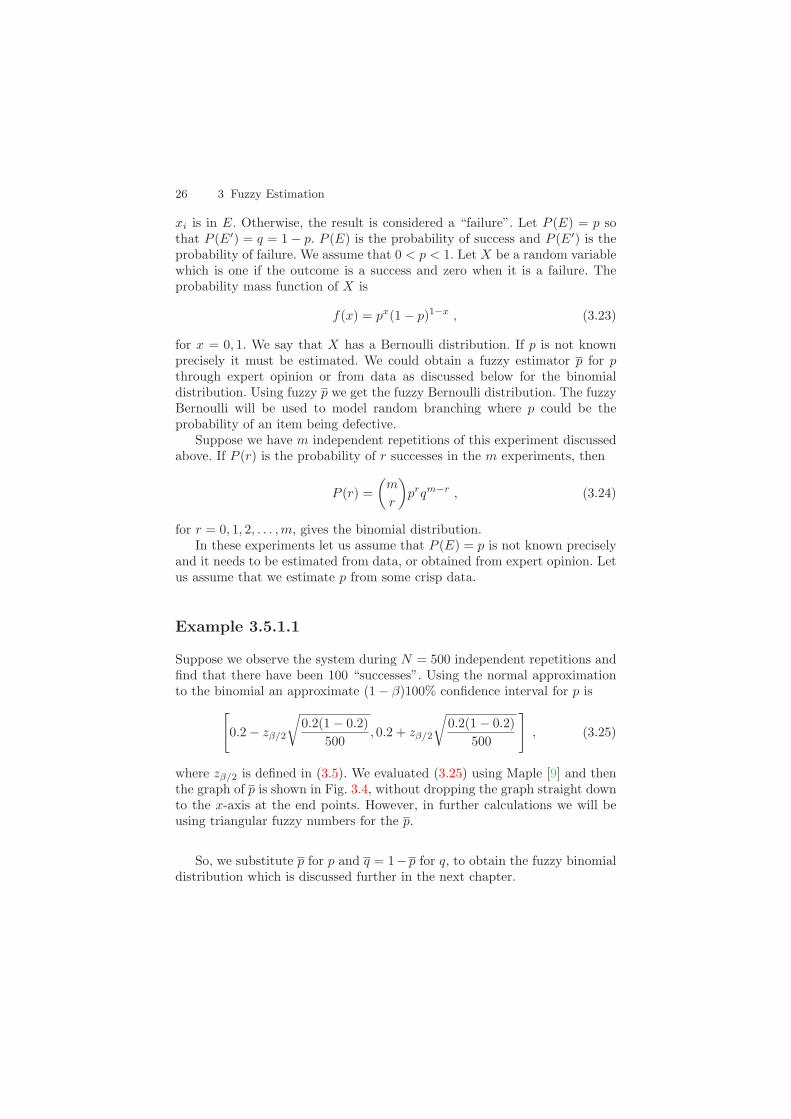
Example 3.5.1.1
Suppose we observe the system during N = 500 independent repetitions andfind that there have been 100 “successes”. Using the normal approximationto the binomial an approximate (1 − β)100% confidence interval for p is
[0.2 − zβ/2
√0.2(1 − 0.2)
500, 0.2 + zβ/2
√0.2(1 − 0.2)
500
], (3.25)
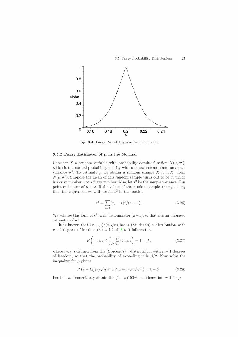
where zβ/2 is defined in (3.5). We evaluated (3.25) using Maple [9] and thenthe graph of p is shown in Fig. 3.4, without dropping the graph straight downto the x-axis at the end points. However, in further calculations we will beusing triangular fuzzy numbers for the p.
So, we substitute p for p and q = 1− p for q, to obtain the fuzzy binomialdistribution which is discussed further in the next chapter.
3.5 Fuzzy Probability Distributions 27
0
0.2
0.4
0.6
0.8
1
alpha
0.16 0.18 0.2 0.22 0.24x
Fig. 3.4. Fuzzy Probability p in Example 3.5.1.1
3.5.2 Fuzzy Estimator of µ in the Normal
Consider X a random variable with probability density function N(µ, σ2),which is the normal probability density with unknown mean µ and unknownvariance σ2. To estimate µ we obtain a random sample X1, . . . , Xn fromN(µ, σ2). Suppose the mean of this random sample turns out to be x, whichis a crisp number, not a fuzzy number. Also, let s2 be the sample variance. Ourpoint estimator of µ is x. If the values of the random sample are x1, . . . , xn
then the expression we will use for s2 in this book is
s2 =n∑
i=1
(xi − x)2/(n − 1) . (3.26)
We will use this form of s2, with denominator (n−1), so that it is an unbiasedestimator of σ2.
It is known that (x − µ)/(s/√
n) has a (Student’s) t distribution withn − 1 degrees of freedom (Sect. 7.2 of [8]). It follows that
P
(−tβ/2 ≤ x − µ
s/√
n≤ tβ/2
)= 1 − β , (3.27)
where tβ/2 is defined from the (Student’s) t distribution, with n − 1 degreesof freedom, so that the probability of exceeding it is β/2. Now solve theinequality for µ giving
P(x − tβ/2s/
√n ≤ µ ≤ x + tβ/2s/
√n)
= 1 − β . (3.28)
For this we immediately obtain the (1 − β)100% confidence interval for µ

28 3 Fuzzy Estimation
[x − tβ/2s/
√n, x + tβ/2s/
√n]
. (3.29)
Put these confidence intervals together, as discussed in Sect. 3.3, and weobtain µ our fuzzy number estimator of µ.
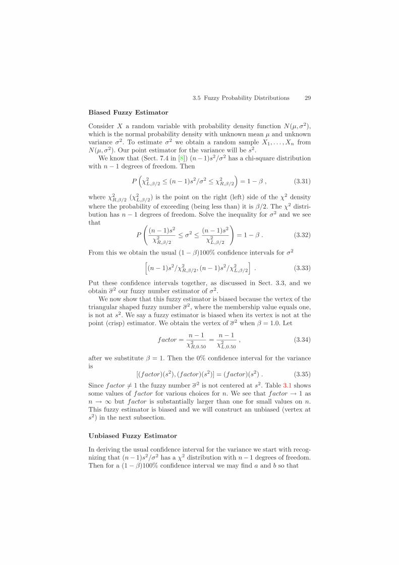
Example 3.5.2.1
Consider X a random variable with probability density function N(µ, σ2),which is the normal probability density with unknown mean µ and unknownvariance σ2. To estimate µ we obtain a random sample X1, . . . , Xn fromN(µ, σ2). Suppose the mean of this random sample of size 25 turns out to be28.6 and s2 = 3.42. Then a (1 − β)100% confidence interval for µ is[
28.6 − tβ/2
√3.42/25, 28.6 + tβ/2
√3.42/25
]. (3.30)
To obtain a graph of fuzzy µ, or µ, assume that 0.01 ≤ β ≤ 1. We evaluated(3.30) using Maple [9] and then the graph of µ is shown in Fig. 3.5, withoutdropping the graph straight down to the x-axis at the end points.
To complete the picture we draw short vertical line segments, from thehorizontal axis up to the graph, at the end points of the base of the fuzzynumber µ. The base (µ[0]) is a 99% confidence interval for µ.
3.5.3 Fuzzy Estimator of σ2 in the Normal
We first construct a fuzzy estimator for σ2 using the usual confidence intervalsfor the variance from a normal distribution and we show this fuzzy estimatoris biased. Then we construct an unbiased fuzzy estimator for the variance.
0
0.2
0.4
0.6
0.8
1
alpha
28 28.5 29 29.5x
Fig. 3.5. Fuzzy Estimator µ in Example 3.5.2.1
3.5 Fuzzy Probability Distributions 29
Biased Fuzzy Estimator
Consider X a random variable with probability density function N(µ, σ2),which is the normal probability density with unknown mean µ and unknownvariance σ2. To estimate σ2 we obtain a random sample X1, . . . , Xn fromN(µ, σ2). Our point estimator for the variance will be s2.
We know that (Sect. 7.4 in [8]) (n− 1)s2/σ2 has a chi-square distributionwith n − 1 degrees of freedom. Then
P(χ2
L,β/2 ≤ (n − 1)s2/σ2 ≤ χ2R,β/2
)= 1 − β , (3.31)
where χ2R,β/2 (χ2
L,β/2) is the point on the right (left) side of the χ2 densitywhere the probability of exceeding (being less than) it is β/2. The χ2 distri-bution has n − 1 degrees of freedom. Solve the inequality for σ2 and we seethat
P
((n − 1)s2
χ2R,β/2
≤ σ2 ≤ (n − 1)s2
χ2L,β/2
)= 1 − β . (3.32)
From this we obtain the usual (1 − β)100% confidence intervals for σ2
[(n − 1)s2/χ2
R,β/2, (n − 1)s2/χ2L,β/2
]. (3.33)
Put these confidence intervals together, as discussed in Sect. 3.3, and weobtain σ2 our fuzzy number estimator of σ2.
We now show that this fuzzy estimator is biased because the vertex of thetriangular shaped fuzzy number σ2, where the membership value equals one,is not at s2. We say a fuzzy estimator is biased when its vertex is not at thepoint (crisp) estimator. We obtain the vertex of σ2 when β = 1.0. Let
factor =n − 1χ2
R,0.50
=n − 1χ2
L,0.50
, (3.34)
after we substitute β = 1. Then the 0% confidence interval for the varianceis
[(factor)(s2), (factor)(s2)] = (factor)(s2) . (3.35)
Since factor = 1 the fuzzy number σ2 is not centered at s2. Table 3.1 showssome values of factor for various choices for n. We see that factor → 1 asn → ∞ but factor is substantially larger than one for small values on n.This fuzzy estimator is biased and we will construct an unbiased (vertex ats2) in the next subsection.
Unbiased Fuzzy Estimator
In deriving the usual confidence interval for the variance we start with recog-nizing that (n− 1)s2/σ2 has a χ2 distribution with n− 1 degrees of freedom.Then for a (1 − β)100% confidence interval we may find a and b so that
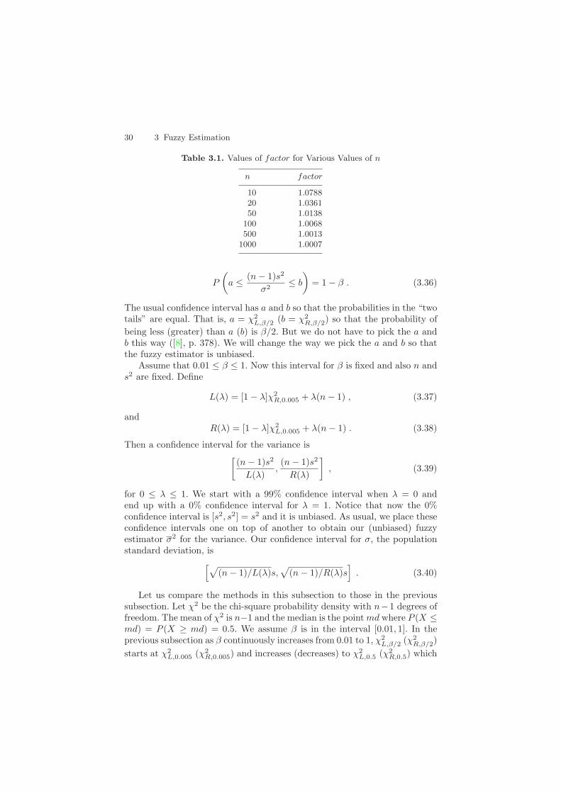
30 3 Fuzzy Estimation
Table 3.1. Values of factor for Various Values of n
n factor
10 1.078820 1.036150 1.0138
100 1.0068500 1.0013
1000 1.0007
P
(a ≤ (n − 1)s2
σ2≤ b
)= 1 − β . (3.36)
The usual confidence interval has a and b so that the probabilities in the “twotails” are equal. That is, a = χ2
L,β/2 (b = χ2R,β/2) so that the probability of
being less (greater) than a (b) is β/2. But we do not have to pick the a andb this way ([8], p. 378). We will change the way we pick the a and b so thatthe fuzzy estimator is unbiased.
Assume that 0.01 ≤ β ≤ 1. Now this interval for β is fixed and also n ands2 are fixed. Define
L(λ) = [1 − λ]χ2R,0.005 + λ(n − 1) , (3.37)
andR(λ) = [1 − λ]χ2
L,0.005 + λ(n − 1) . (3.38)
Then a confidence interval for the variance is[(n − 1)s2
L(λ),(n − 1)s2
R(λ)
], (3.39)
for 0 ≤ λ ≤ 1. We start with a 99% confidence interval when λ = 0 andend up with a 0% confidence interval for λ = 1. Notice that now the 0%confidence interval is [s2, s2] = s2 and it is unbiased. As usual, we place theseconfidence intervals one on top of another to obtain our (unbiased) fuzzyestimator σ2 for the variance. Our confidence interval for σ, the populationstandard deviation, is
[√(n − 1)/L(λ)s,
√(n − 1)/R(λ)s
]. (3.40)
Let us compare the methods in this subsection to those in the previoussubsection. Let χ2 be the chi-square probability density with n−1 degrees offreedom. The mean of χ2 is n−1 and the median is the point md where P (X ≤md) = P (X ≥ md) = 0.5. We assume β is in the interval [0.01, 1]. In theprevious subsection as β continuously increases from 0.01 to 1, χ2
L,β/2 (χ2R,β/2)
starts at χ2L,0.005 (χ2
R,0.005) and increases (decreases) to χ2L,0.5 (χ2
R,0.5) which

3.5 Fuzzy Probability Distributions 31
equals to the median. Recall that χ2L,β/2 (χ2
R,β/2) is the point on the χ2
density where the probability of being less (greater) that it equals β/2. FromTable 3.1 we see that the median is always less than n − 1. This producesthe bias in the fuzzy estimator in that subsection. In this subsection as λcontinuously increases from zero to one L(λ) (R(λ)) decreases (increases)from χ2
R,0.005 (χ2L,0.005) to n − 1. At λ = 1 we get L(1) = R(1) = n − 1 and
the vertex (membership value one) is at s2 and it is now unbiased.We will use this fuzzy estimator σ2 constructed in this section for σ2 in
the rest of this book. Given a value of λ = λ∗ ∈ [0, 1] one may wonder whatis the corresponding value of β for the confidence interval. We now show howto get the β. Let L∗ = L(λ∗) and R∗ = R(λ∗). Define
l =∫ R∗
0
χ2dx , (3.41)
andr =
∫ ∞
L∗χ2dx , (3.42)
and then β = l + r. Now l (r) need not equal β/2. Both of these integralsabove are easily evaluated using Maple [9]. The chi-square density inside theseintegrals has n − 1 degrees of freedom.
Example 3.5.3.1
Consider X a random variable with probability density function N(µ, σ2),which is the normal probability density with mean µ and unknown varianceσ2. To estimate σ2 we obtain a random sample X1, . . . , Xn from N(µ, σ2).Suppose n = 25 and we calculate s2 = 3.42. Then a confidence interval forσ2 is [
82.08L(λ)
,82.08R(λ)
]. (3.43)
To obtain a graph of fuzzy σ2, or σ2, first assume that 0.01 ≤ β ≤ 1. Weevaluated (3.43) using Maple [9] and then the graph of σ2 is shown in Fig. 3.6,without dropping the graph straight down to the x-axis at the end points.
To complete the picture we draw short vertical line segments, from thehorizontal axis up to the graph, at the end points of the base of the fuzzynumber σ2. The base (σ2[0]) is a 99% confidence interval for σ2.
To complete this subsection let us present one graph of our fuzzy estimatorσ of σ. Alpha-cuts of σ are [
9.06√L(λ)
,9.06√R(λ)
]. (3.44)
Assuming 0.01 ≤ β ≤ 1, the graph is in Fig. 3.7.
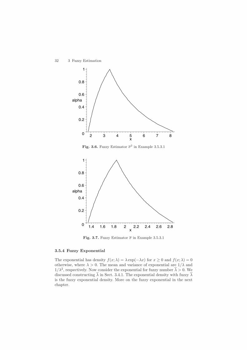
32 3 Fuzzy Estimation
0
0.2
0.4
0.6
0.8
1
alpha
2 3 4 5 6 7 8x
Fig. 3.6. Fuzzy Estimator σ2 in Example 3.5.3.1
0
0.2
0.4
0.6
0.8
1
alpha
1.4 1.6 1.8 2 2.2 2.4 2.6 2.8x
Fig. 3.7. Fuzzy Estimator σ in Example 3.5.3.1
3.5.4 Fuzzy Exponential
The exponential has density f(x;λ) = λ exp(−λx) for x ≥ 0 and f(x;λ) = 0otherwise, where λ > 0. The mean and variance of exponential are 1/λ and1/λ2, respectively. Now consider the exponential for fuzzy number λ > 0. Wediscussed constructing λ in Sect. 3.4.1. The exponential density with fuzzy λis the fuzzy exponential density. More on the fuzzy exponential in the nextchapter.

3.5 Fuzzy Probability Distributions 33
3.5.5 Fuzzy Uniform
Let U(a, b), for 0 ≤ a < b, denote the uniform distribution whose densityfunction is f(x) = 1/(b − a) for a < x < b, and f(x) = 0 otherwise. Theuniform distribution will be used to model times between arrivals in a queuingsystem and/or service times in a server.
Assume that we do not know a and b precisely so they must be estimated.Let X1, . . . , Xn be a random sample from U(a, b) and let x1, . . . , xn be thevalues of this random sample. Define xmin = minxi|1 ≤ i ≤ n and xmax =maxxi|1 ≤ i ≤ n. Then xmin (xmax) is our point estimator of a (b). We maynow construct (1 − β)100% confidence intervals for a (b), for 0.01 ≤ β ≤ 1,and placing these intervals one on top of another (with completing the baseas described above) to obtain our fuzzy estimator a (b) of a (b). We willnot describe the mechanics of building these confidence intervals in this bookbecause to do so would divert us into too much theoretical work in probabilityand statistics. The solution for the confidence intervals is complicated [10]and not to be found in statistics books. However, we do show the resultsin Figs. 3.8 and 3.9. Both figures give a and b and in Fig. 3.8 the left sideof a was cut off because a is non-negative. These graphs were done usingMaple [9].
In some applications (Chaps. 12, 14 and 19) we will use triangular fuzzynumbers for a and b. This is not correct since the a and b in Figs. 3.8 and3.9 are not triangular fuzzy numbers. It is just a habit of the author to usetriangular fuzzy numbers in applications. However, changing the a and b inthese chapters to look like those in Figs. 3.8 and 3.9 would probably onlycause small changes in the results.
0 1xmin
a 2 3xmax
b 4 5x
1
a b
y
Fig. 3.8. Fuzzy Estimators a and b in U(a, b)
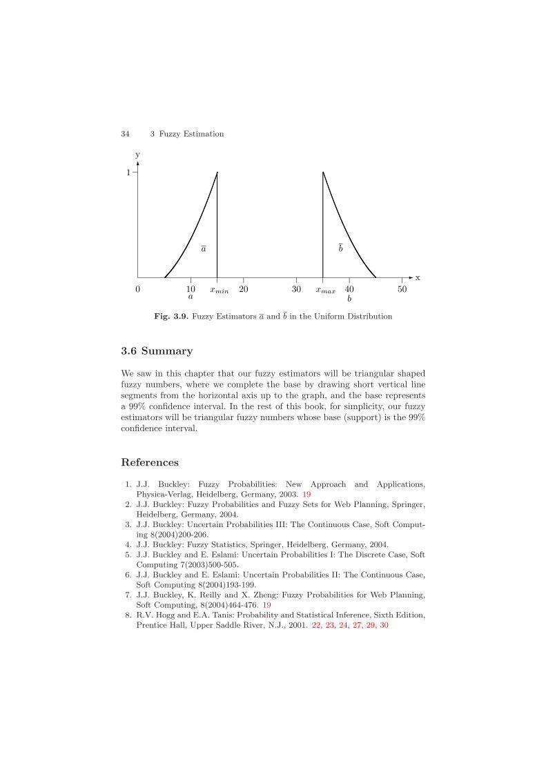
34 3 Fuzzy Estimation
0 10 xmina
20 30 xmax 40b
50x
1
a b
y
Fig. 3.9. Fuzzy Estimators a and b in the Uniform Distribution
3.6 Summary
We saw in this chapter that our fuzzy estimators will be triangular shapedfuzzy numbers, where we complete the base by drawing short vertical linesegments from the horizontal axis up to the graph, and the base representsa 99% confidence interval. In the rest of this book, for simplicity, our fuzzyestimators will be triangular fuzzy numbers whose base (support) is the 99%confidence interval.
References
1. J.J. Buckley: Fuzzy Probabilities: New Approach and Applications,Physica-Verlag, Heidelberg, Germany, 2003. 19
2. J.J. Buckley: Fuzzy Probabilities and Fuzzy Sets for Web Planning, Springer,Heidelberg, Germany, 2004.
3. J.J. Buckley: Uncertain Probabilities III: The Continuous Case, Soft Comput-ing 8(2004)200-206.
4. J.J. Buckley: Fuzzy Statistics, Springer, Heidelberg, Germany, 2004.5. J.J. Buckley and E. Eslami: Uncertain Probabilities I: The Discrete Case, Soft
Computing 7(2003)500-505.6. J.J. Buckley and E. Eslami: Uncertain Probabilities II: The Continuous Case,
Soft Computing 8(2004)193-199.7. J.J. Buckley, K. Reilly and X. Zheng: Fuzzy Probabilities for Web Planning,
Soft Computing, 8(2004)464-476. 198. R.V. Hogg and E.A. Tanis: Probability and Statistical Inference, Sixth Edition,
Prentice Hall, Upper Saddle River, N.J., 2001. 22, 23, 24, 27, 29, 30

References 35
9. Maple 9, Waterloo Maple Inc., Waterloo, Canada. 21, 23, 25, 26, 28, 31, 3310. Personal Communication from Professor N. Chernov, Mathematics Depart-
ment, UAB, Birmingham, Alabama. 3311. H.A. Taha: Operations Research, Fifth Edition, Macmillan, N.Y., 1992. 20, 22, 23

4 Fuzzy Probability Theory
4.1 Introduction
In this chapter we look more closely at the fuzzy binomial distribution, thefuzzy Poisson, and at the fuzzy normal, exponential and uniform densities.We need to be familiar with these fuzzy probability functions because theiruse transforms crisp systems theory to fuzzy system theory (Chap. 5). Thematerial in this chapter is based on [1, 2, 3, 4].
4.2 Fuzzy Binomial
As before X = x1, . . . , xn and let E be a non-empty, proper, subset ofX. We have an experiment where the result is considered a “success” if theoutcome xi is in E. Otherwise, the result is considered a “failure”. Let P (E) =p so that P (E′) = q = 1− p. P (E) is the probability of success and P (E′) isthe probability of failure. We assume that 0 < p < 1.
Suppose we have m independent repetitions of this experiment. If P (r) isthe probability of r successes in the m experiments, then
P (r) =(
m
r
)prqm−r , (4.1)
for r = 0, 1, 2, . . . ,m, gives the binomial distribution.In these experiments let us assume that P (E) is not known precisely and
it needs to be estimated, or obtained from expert opinion. So the p value isuncertain and we substitute p for p (see Sect. 3.5.1) and q = 1 − p. Now letP (r) be the fuzzy probability of r successes in m independent trials of theexperiment. Then we obtain
P (r)[α] =(
m
r
)prqm−r|S
, (4.2)
for 0 ≤ α ≤ 1, where S is the statement “p ∈ p[α], q ∈ q[α], p+ q = 1”. Thereis uncertainty in the value of p and q but there is no uncertainty in the factthat the sum of p and q must equal one. Notice that P (r) is not
(mr
)prqm−r.
If P (r)[α] = [Pr1(α), Pr2(α)], then
James J. Buckley: Simulating Fuzzy Systems, StudFuzz 171, 37–48 (2005)www.springerlink.com c© Springer-Verlag Berlin Heidelberg 2005
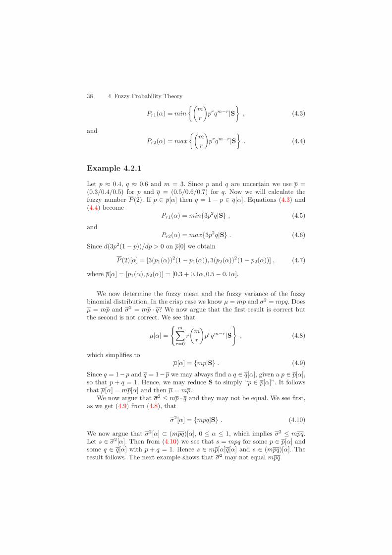
38 4 Fuzzy Probability Theory
Pr1(α) = min
(m
r
)prqm−r|S
, (4.3)
and
Pr2(α) = max
(m
r
)prqm−r|S
. (4.4)
Example 4.2.1
Let p ≈ 0.4, q ≈ 0.6 and m = 3. Since p and q are uncertain we use p =(0.3/0.4/0.5) for p and q = (0.5/0.6/0.7) for q. Now we will calculate thefuzzy number P (2). If p ∈ p[α] then q = 1 − p ∈ q[α]. Equations (4.3) and(4.4) become
Pr1(α) = min3p2q|S , (4.5)
andPr2(α) = max3p2q|S . (4.6)
Since d(3p2(1 − p))/dp > 0 on p[0] we obtain
P (2)[α] = [3(p1(α))2(1 − p1(α)), 3(p2(α))2(1 − p2(α))] , (4.7)
where p[α] = [p1(α), p2(α)] = [0.3 + 0.1α, 0.5 − 0.1α].
We now determine the fuzzy mean and the fuzzy variance of the fuzzybinomial distribution. In the crisp case we know µ = mp and σ2 = mpq. Doesµ = mp and σ2 = mp · q? We now argue that the first result is correct butthe second is not correct. We see that
µ[α] =
m∑
r=0
r
(m
r
)prqm−r|S
, (4.8)
which simplifies toµ[α] = mp|S . (4.9)
Since q = 1−p and q = 1−p we may always find a q ∈ q[α], given a p ∈ p[α],so that p + q = 1. Hence, we may reduce S to simply “p ∈ p[α]”. It followsthat µ[α] = mp[α] and then µ = mp.
We now argue that σ2 ≤ mp · q and they may not be equal. We see first,as we get (4.9) from (4.8), that
σ2[α] = mpq|S . (4.10)
We now argue that σ2[α] ⊂ (mpq)[α], 0 ≤ α ≤ 1, which implies σ2 ≤ mpq.Let s ∈ σ2[α]. Then from (4.10) we see that s = mpq for some p ∈ p[α] andsome q ∈ q[α] with p + q = 1. Hence s ∈ mp[α]q[α] and s ∈ (mpq)[α]. Theresult follows. The next example shows that σ2 may not equal mpq.

4.3 Fuzzy Poisson 39
Example 4.2.2
Let p = (0.4/0.6/0.8) and q = 1 − p = (0.2/0.4/0.6). If p is in p[α], then wecan always choose q = 1 − p ∈ q[α] so that p + q = 1. Then
σ2[α] = mp(1 − p)|p ∈ p[α] , (4.11)
from (4.10). Let h(p) = mp(1 − p). We see that h(p): (1) is increasing on[0, 0.5]; (2) has its maximum of 0.25 m at p = 0.5; and (3) is decreasing on[0.5, 1]. So, the evaluation of (4.11) depends if p = 0.5 belongs to the α-cutof p. Let p[α] = [p1(α), p2(α)] = [0.4 + 0.2α, 0.8 − 0.2α]. So, p = 0.5 belongsto the α-cut of p only for 0 ≤ α ≤ 0.5. Then
σ2[α] = [h(p2(α)), 0.25m] , (4.12)
for 0 ≤ α ≤ 0.5, and
σ2[α] = [h(p2(α)), h(p1(α))] , (4.13)
for 0.5 ≤ α ≤ 1. We substitute in for p1(α) and p2(α) to finally obtain σ2
and its graph, for m = 10, using Maple [5] is in Fig. 4.1. Clearly σ2 does notequal 10pq. For example σ2[0] = [1.6, 2.5] but (10pq)[0] = [0.8, 4.8].
4.3 Fuzzy Poisson
Let X be a random variable having the Poisson probability mass function. IfP (x) stands for the probability that X = x, then
0
0.2
0.4
0.6
0.8
1
alpha
1.6 1.8 2 2.2 2.4x
Fig. 4.1. Fuzzy Variance in Example 4.2.2

40 4 Fuzzy Probability Theory
P (x) =λx exp(−λ)
x!, (4.14)
for x = 0, 1, 2, 3, . . . , and parameter λ > 0. Now λ is not known precisely andmust be estimated from some (crisp) data. See Sect. 3.4.1. Our estimator isa fuzzy number so substitute this fuzzy number λ > 0 for λ to produce thefuzzy Poisson probability mass function. Set P (x) to be the fuzzy probabilitythat X = x. Then we find α-cuts of this fuzzy number as
P (x)[α] =
λx exp(−λ)x!
|λ ∈ λ[α]
, (4.15)
for all α ∈ [0, 1]. The evaluation of (4.15) depends on the relation of x to λ[0].Let h(λ) = λx exp(−λ)
x! for fixed x and λ > 0. We see that h(λ) is an increasingfunction of λ for λ < x, the maximum value of h(λ) occurs at λ = x, and h(λ)is a decreasing function of λ for λ > x. Let λ[α] = [λ1(α), λ2(α)], for 0 ≤ α ≤1. Then we see that: (1) if λ2(0) < x, then P (x)[α] = [h(λ1(α)), h(λ2(α))];and (2) if x < λ1(0), then P (x)[α] = [h(λ2(α)), h(λ1(α))]. The other case,where x ∈ λ[0], is explored in the following example.
Example 4.3.1
Let x = 6 and λ = (3/5/7). We see that x ∈ [3, 7] = λ[0]. We determineλ[α] = [3 + 2α, 7 − 2α]. Define P (6)[α] = [p1(α), p2(α)]. To determine theα-cuts of P (6) we need to solve (see Sect. 2.4.1)
p1(α) = minh(λ)|λ ∈ λ[α] , (4.16)
andp2(α) = maxh(λ)|λ ∈ λ[α] . (4.17)
It is not difficult to solve (4.16) and (4.17) producing
P (6)[α] = [h(3 + 2α), h(6)] , (4.18)
for 0 ≤ α ≤ 0.5, and
P (6)[α] = [h(3 + 2α), h(7 − 2α)] , (4.19)
for 0.5 ≤ α ≤ 1. The graph of P (6) is shown in Fig. 4.2.Let us consider another, slightly more complicated, example of finding
fuzzy probabilities using the fuzzy Poisson.
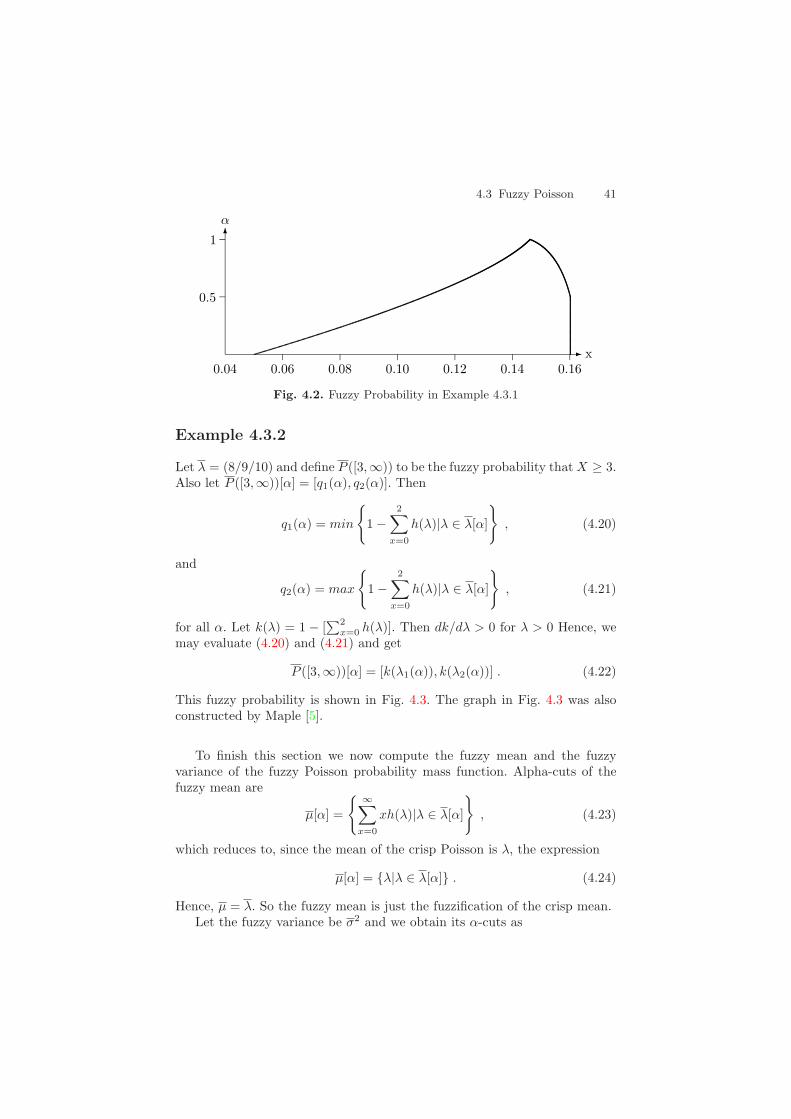
4.3 Fuzzy Poisson 41
0.04 0.06 0.08 0.10 0.12 0.14 0.16x
1
0.5
α
Fig. 4.2. Fuzzy Probability in Example 4.3.1
Example 4.3.2
Let λ = (8/9/10) and define P ([3,∞)) to be the fuzzy probability that X ≥ 3.Also let P ([3,∞))[α] = [q1(α), q2(α)]. Then
q1(α) = min
1 −
2∑x=0
h(λ)|λ ∈ λ[α]
, (4.20)
and
q2(α) = max
1 −
2∑x=0
h(λ)|λ ∈ λ[α]
, (4.21)
for all α. Let k(λ) = 1 − [∑2
x=0 h(λ)]. Then dk/dλ > 0 for λ > 0 Hence, wemay evaluate (4.20) and (4.21) and get
P ([3,∞))[α] = [k(λ1(α)), k(λ2(α))] . (4.22)
This fuzzy probability is shown in Fig. 4.3. The graph in Fig. 4.3 was alsoconstructed by Maple [5].
To finish this section we now compute the fuzzy mean and the fuzzyvariance of the fuzzy Poisson probability mass function. Alpha-cuts of thefuzzy mean are
µ[α] =
∞∑x=0
xh(λ)|λ ∈ λ[α]
, (4.23)
which reduces to, since the mean of the crisp Poisson is λ, the expression
µ[α] = λ|λ ∈ λ[α] . (4.24)
Hence, µ = λ. So the fuzzy mean is just the fuzzification of the crisp mean.Let the fuzzy variance be σ2 and we obtain its α-cuts as
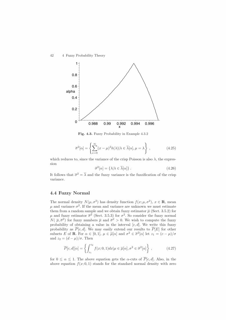
42 4 Fuzzy Probability Theory
0
0.2
0.4
0.6
0.8
1
alpha
0.988 0.99 0.992 0.994 0.996x
Fig. 4.3. Fuzzy Probability in Example 4.3.2
σ2[α] =
∞∑x=0
(x − µ)2h(λ)|λ ∈ λ[α], µ = λ
, (4.25)
which reduces to, since the variance of the crisp Poisson is also λ, the expres-sion
σ2[α] = λ|λ ∈ λ[α] . (4.26)
It follows that σ2 = λ and the fuzzy variance is the fuzzification of the crispvariance.
4.4 Fuzzy Normal
The normal density N(µ, σ2) has density function f(x;µ, σ2), x ∈ R, meanµ and variance σ2. If the mean and variance are unknown we must estimatethem from a random sample and we obtain fuzzy estimator µ (Sect. 3.5.2) forµ and fuzzy estimator σ2 (Sect. 3.5.3) for σ2. So consider the fuzzy normalN( µ, σ2) for fuzzy numbers µ and σ2 > 0. We wish to compute the fuzzyprobability of obtaining a value in the interval [c, d]. We write this fuzzyprobability as P [c, d]. We may easily extend our results to P [E] for othersubsets E of R. For α ∈ [0, 1], µ ∈ µ[α] and σ2 ∈ σ2[α] let z1 = (c − µ)/σand z2 = (d − µ)/σ. Then
P [c, d][α] =∫ z2
z1
f(x; 0, 1)dx|µ ∈ µ[α], σ2 ∈ σ2[α]
, (4.27)
for 0 ≤ α ≤ 1. The above equation gets the α-cuts of P [c, d]. Also, in theabove equation f(x; 0, 1) stands for the standard normal density with zero
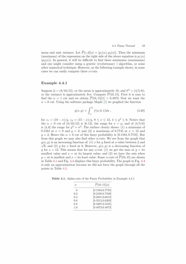
4.4 Fuzzy Normal 43
mean and unit variance. Let P [c, d][α] = [p1(α), p2(α)]. Then the minimum(maximum) of the expression on the right side of the above equation is p1(α)(p2(α)). In general, it will be difficult to find these minimums (maximums)and one might consider using a genetic (evolutionary ) algorithm, or someother numerical technique. However, as the following example shows, in somecases we can easily compute these α-cuts.
Example 4.4.1
Suppose µ = (8/10/12), or the mean is approximately 10, and σ2 = (4/5/6),or the variance is approximately five. Compute P [10, 15]. First it is easy tofind the α = 1 cut and we obtain P [10, 15][1] = 0.4873. Now we want theα = 0 cut. Using the software package Maple [5] we graphed the function
g(x, y) =∫ z2
z1
f(u; 0, 1)du , (4.28)
for z1 = (10 − x)/y, z2 = (15 − x)/y, 8 ≤ x ≤ 12, 4 ≤ y2 ≤ 6. Notice thatthe α = 0 cut of (8/10/12) is [8, 12], the range for x = µ, and of (4/5/6)is [4, 6] the range for y2 = σ2. The surface clearly shows: (1) a minimum of0.1584 at x = 8 and y = 2; and (2) a maximum of 0.7745 at x = 12 andy = 2. Hence the α = 0 cut of this fuzzy probability is [0.1584, 0.7745]. Butfrom this graph we may also find other α-cuts. We see from the graph thatg(x, y) is an increasing function of: (1) x for y fixed at a value between 2 and√
6; and (2) y for x fixed at 8. However, g(x, y) is a decreasing function ofy for x = 12. This means that for any α-cut: (1) we get the max at y = itssmallest value and x = at its largest value; and (2) we have the min wheny = at is smallest and x = its least value. Some α-cuts of P [10, 15] are shownin Table 4.1 and Fig. 4.4 displays this fuzzy probability. The graph in Fig. 4.4is only an approximation because we did not force the graph through all thepoints in Table 4.1.
Table 4.1. Alpha-cuts of the Fuzzy Probability in Example 4.4.1
α P [10, 15][α]
0 [0.1584,0.7745]0.2 [0.2168,0.7340]0.4 [0.2821,0,6813]0.6 [0.3512,0.6203]0.8 [0.4207,0.5545]1.0 [0.4873,0.4873]

44 4 Fuzzy Probability Theory
0 0.2 0.4 0.6 0.8 1x
1
α
Fig. 4.4. Approximate Fuzzy Probability in Example 4.4.1
We now show that the fuzzy mean of N(µ, σ2) is µ and the fuzzy varianceis σ2, respectively, the fuzzification of the crisp mean and variance. Let thefuzzy mean be M . Then its α-cuts are
M [α] =∫ ∞
−∞xf(x;µ, σ2)dx|µ ∈ µ[α], σ2 ∈ σ2[α]
. (4.29)
But the integral in the above equation equals µ for any µ ∈ µ[α] and anyσ2 ∈ σ2[α]. Hence M = µ. Let the fuzzy variance be V . Then its α-cuts are
V [α] =∫ ∞
−∞(x − µ)2f(x, µ, σ2)dx|µ ∈ µ[α], σ2 ∈ σ2[α]
. (4.30)
We see that the integral in the above equation equals σ2 for all µ ∈ µ[α] andall σ2 ∈ σ2[α]. Therefore, V = σ2.
4.5 Fuzzy Exponential
The exponential E(λ) has density f(x;λ) = λ exp(−λx) for x ≥ 0 andf(x;λ) = 0 otherwise, where λ > 0. The mean and variance of E(λ) is1/λ and 1/λ2, respectively. If the parameter λ is unknown we estimate itfrom some random sample producing fuzzy estimator λ (Sect. 3.4.2) for λ.Now consider E(λ) for fuzzy number λ > 0. Let us find the fuzzy probabilityof obtaining a value in the interval [c, d], c > 0. Denote this probability asP [c, d]. One may generalize to P [E] for other subsets E of R. We compute
P [c, d][α] =
∫ d
c
λ exp(−λx)dx|λ ∈ λ[α]
, (4.31)

4.5 Fuzzy Exponential 45
for all α. Let P [c, d][α] = [p1(α), p2(α)], then
p1(α) = min
∫ d
c
λ exp(−λx)dx|λ ∈ λ[α]
, (4.32)
and
p2(α) = max
∫ d
c
λ exp(−λx)dx|λ ∈ λ[α]
, (4.33)
for 0 ≤ α ≤ 1. Let
h(λ) = exp(−cλ) − exp(−dλ) =∫ d
c
λ exp(−λx)dx , (4.34)
and we see that h: (1) is an increasing function of λ for 0 < λ < λ∗; and (2) is adecreasing function of λ for λ∗ < λ. We find that λ∗ = −[ln(c/d)]/(d−c). As-sume that λ > λ∗. So we can now easily find P [c, d]. Let λ[α] = [λ1(α), λ2(α)].Then
p1(α) = h(λ2(α)) , (4.35)
andp2(α) = h(λ1(α)) . (4.36)
We give a picture of this fuzzy probability, using Maple [5], in Fig. 4.5 when:(1) c = 1 and d = 4; and (2) λ = (1/3/5).
Next we find the fuzzy mean and fuzzy variance of E(λ). If µ denotes themean, we find its α-cuts as
0
0.2
0.4
0.6
0.8
1
alpha
0.05 0.1 0.15 0.2 0.25 0.3 0.35x
Fig. 4.5. Fuzzy Probability for the Fuzzy Exponential

46 4 Fuzzy Probability Theory
µ[α] =∫ ∞
0
xλ exp(−λx)dx|λ ∈ λ[α]
, (4.37)
for all α. However, each integral in the above equation equals 1/λ. Henceµ = 1/λ. If σ2 is the fuzzy variance, then we write down an equation to findits α-cuts we obtain σ2 = 1/λ
2. The fuzzy mean (variance) is the fuzzification
of the crisp mean (variance).
4.6 Fuzzy Uniform
The uniform density U(a, b), a < b, has density function y = f(x; a, b) =1/(b− a) for a < x < b and f(x; a, b) = 0 otherwise. Now consider U(a, b) forfuzzy numbers a and b. In this section we will model a and b as triangularfuzzy numbers. Notice that in Sect. 3.5.5 a and b were half of a triangularshaped fuzzy number as shown in Fig. 3.9 and the left side of a got cut offin Fig. 3.8. The fuzzy sets in Figs. 3.8 and 3.9 are what we should use inthe rest of the book but for now let us have triangular fuzzy numbers fora and b. Assume that a[1] = a and b[1] = b so that a ( b ) represents theuncertainty in a (b). Now using the fuzzy uniform density we wish to computethe fuzzy probability of obtaining a value in the interval [c, d]. Denote thisfuzzy probability as P [c, d]. We can easily generalize to P [E] for more generalsubsets E.
There is uncertainty in the end points of the uniform density but thereis no uncertainty in the fact that we have a uniform density. What thismeans is that given any s ∈ a[α] and t ∈ b[α], s < t, we have a U(s, t), orf(x; s, t) = 1/(t − s) on [s, t] and it equals zero otherwise, for all 0 ≤ α ≤ 1.This enables us to find fuzzy probabilities. Let L(c, d; s, t) be the length ofthe interval [s, t] ∩ [c, d]. Then
P [c, d][α] = L(c, d; s, t)/(t − s)|s ∈ a[α], t ∈ b[α], s < t , (4.38)
for all α ∈ [0, 1]. Equation (4.38) defines the α-cuts and we put these α-cutstogether to obtain the fuzzy set P [c, d]. To find an α-cut of P [c, d] we find theprobability of getting a value in the interval [c, d] for each uniform densityU(s, t) for all s ∈ a[α] and all t ∈ b[α], with s < t.
Example 4.6.1
Let a = (0/1/2) and b = (3/4/5) and [c, d] = [1, 4]. Now P [c, d][α] =[p1(α), p2(α)] an interval whose end points are functions of α. Then p1(α)is the minimum value of the expression on the right side of (4.38) and p2(α)is the maximum value. That is
p1(α) = minL(1, 4; s, t)/(t − s)|s ∈ a[α], t ∈ b[α] , (4.39)

4.6 Fuzzy Uniform 47
0.6 0.7 0.8 0.9 1x
1
y
Fig. 4.6. Fuzzy Probability in Example 4.6.1
andp2(α) = maxL(1, 4; s, t)/(t − s)|s ∈ a[α], t ∈ b[α] . (4.40)
It is easily seen that p2(α) = 1 all α in this example. To find the minimumwe must consider four cases. First a[α] = [α, 2− α] and b[α] = [3 + α, 5− α].Then the cases are: (1) α ≤ s ≤ 1, 3+α ≤ t ≤ 4; (2) α ≤ s ≤ 1, 4 ≤ t ≤ 5−α;(3) 1 ≤ s ≤ 2 − α, 3 + α ≤ t ≤ 4; and (4) 1 ≤ s ≤ 2 − α, 4 ≤ t ≤ 5 − α.Studying all four cases we obtain the minimum equal to 3/(5 − 2α). Hencethe α-cuts of P [1, 4] are [3/(5− 2α), 1] and the graph of this fuzzy number isin Fig. 4.6.
Next we want to find the mean and variance of U(a, b). Let the mean beµ and we find its α-cuts as follows
µ[α] =∫ t
s
(x/(t − s))dx|s ∈ a[α], t ∈ b[α], s < t
, (4.41)
for all α. But each integral in (4.41) equals (s + t)/2. Hence, assuming a[0] =[s1, s2], b[0] = [t1, t2] and s2 < t1,
µ = (a + b)/2 . (4.42)
So, µ is the fuzzification of the crisp mean (a + b)/2. If the variance of U(a, b)is σ2, then its α-cuts are
σ2[α] =∫ t
s
[(x − µ)2/(t − s)]dx|s ∈ a[α], t ∈ b[α], µ = (s + t)/2, s < t
,
(4.43)

48 4 Fuzzy Probability Theory
for all α. Each integral in (4.43) equals (t − s)2/12. Hence σ2 = (b − a)2/12,the fuzzification of the crisp variance.
References
1. J.J. Buckley: Fuzzy Probabilities: New Approach and Applications,Physica-Verlag, Heidelberg, Germany, 2003. 37
2. J.J. Buckley: Uncertain Probabilities III: The Continuous Case, Soft Computing,8(2004)200-206. 37
3. J.J. Buckley and E. Eslami: Uncertain Probabilities I: The Discrete Case, SoftComputing, 7(2003)500-505. 37
4. J.J. Buckley and E. Eslami: Uncertain Probabilities II: The Continuous Case,Soft Computing, 8(2004)193-199. 37
5. Maple 9, Waterloo Maple Inc., Waterloo, Canada. 39, 41, 43, 45
5 Fuzzy Systems Theory
5.1 Introduction
In this chapter we consider systems whose performance depends on probabil-ity distributions and some of the parameters in these probability distributionsare to be estimated. We argue that all such systems become fuzzy systemswhose performance will depend on fuzzy probability distributions and whosemeasures of performance can be described by fuzzy numbers. This chapter isbased on [1].
We will consider one example to illustrate our argument. This example,of a queuing network, is shown in Fig. 5.1. We first describe the crisp (non-fuzzy) system in Fig. 5.1 and then, in the next section, we discuss why, andhow, it becomes fuzzy. A brief discussion on how simulation may be used toestimate fuzzy measures of system performance is in Sect. 5.3.
Items arrive at the arrival node according to the exponential distributionwith mean 1.5 minutes. Time within the system will be measured in minutes.These items go immediately to queue number one (Q1 in Fig. 5.1). This queueis assumed to have unlimited capacity so that we never loose an arrival dueto the system being full. All queues can have any queue discipline (first come,first served; priority, etc.). The first server in the system is labelled S1. Anitem from Q1 enters S1 when S1 is available. All service times are assumed tobe normally distributed. Let N(µ, σ2) be the normal distribution with meanµ and variance σ2. So assume that N(µ1, σ
21) describes the service time for
S1. For all N(µ, σ2) used for service time we assume that µ − 5σ2 > 0 sothat we will not be able to randomly generate negative service times usingthe normal distribution.
After service in S1 the item enters the queue Q2 for the next servers S2. Allother queues (Qi, i = 2,3,4,5) in Fig. 5.1 have finite capacity. If Q2 is full, thenan item in S1 can not leave S1, even though its service there is completed, untilthere is space for it in Q2. S2 consists of two parallel and identical servers S21and S22 both with service times N(µ2, σ
22). After completing service in S21 or
S22 the item goes to queue Q3 for server S3 whose service time is N(µ3, σ23).
Then on to Q4 and three parallel and identical servers S41, S42, S43 eachwith service time N(µ4, σ
24). Next is Q5 for the inspection service stations
S51 and S52. The inspector at S51 is more experienced and faster than theinspector at S52 so: (1) Q5 always feeds S51 first if it is available; and (2) Q5
James J. Buckley: Simulating Fuzzy Systems, StudFuzz 171, 49–52 (2005)www.springerlink.com c© Springer-Verlag Berlin Heidelberg 2005
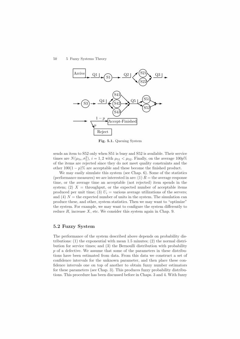
50 5 Fuzzy Systems Theory
Arrive Q1
S1 Q2
S21
S22
Q3
S3 Q4
S41
S42
S43
Q5
S51
S52
Accept-Finished
Reject
1 − p
p
Fig. 5.1. Queuing System
sends an item to S52 only when S51 is busy and S52 is available. Their servicetimes are N(µ5i, σ
25), i = 1, 2 with µ51 < µ52. Finally, on the average 100p%
of the items are rejected since they do not meet quality constraints and theother 100(1 − p)% are acceptable and these become the finished product.
We may easily simulate this system (see Chap. 6). Some of the statistics(performance measures) we are interested in are: (1) R = the average responsetime, or the average time an acceptable (not rejected) item spends in thesystem; (2) X = throughput, or the expected number of acceptable itemsproduced per unit time; (3) Ui = various average utilizations of the servers;and (4) N = the expected number of units in the system. The simulation canproduce these, and other, system statistics. Then we may want to “optimize”the system. For example, we may want to configure the system differently toreduce R, increase X, etc. We consider this system again in Chap. 9.
5.2 Fuzzy System
The performance of the system described above depends on probability dis-tributions: (1) the exponential with mean 1.5 minutes; (2) the normal distri-bution for service times; and (3) the Bernoulli distribution with probabilityp of a defective. We assume that some of the parameters in these distribu-tions have been estimated from data. From this data we construct a set ofconfidence intervals for the unknown parameter, and then place these con-fidence intervals one on top of another to obtain fuzzy number estimatorsfor these parameters (see Chap. 3). This produces fuzzy probability distribu-tions. This procedure has been discussed before in Chaps. 3 and 4. With fuzzy

5.3 Computing Fuzzy Measures of Performance 51
probability distributions we will then compute fuzzy numbers for system per-formance and we have a fuzzy system.
In crisp systems that depend on probability distributions one usually ob-tains point estimates of the parameters in these distributions to be used tocalculate system performance. However, point estimates show no uncertainty.There can be a lot of uncertainty in the model due to these parameters notbeing known precisely.
We suggest adding uncertainty through using fuzzy estimators for the un-known parameters. The fuzzy estimators are constructed from a set of confi-dence intervals. The fuzzy estimators produce fuzzy probability distributionswhich then make the system into a fuzzy system. Hence, many crisp systemsbecome fuzzy systems through this procedure. System performance measureswill now be described by fuzzy numbers which contain the uncertainties fromthe estimation of the parameters in the probability distributions.
Computation of system performance measures becomes much more diffi-cult in the fuzzy system. Assuming the crisp system is sufficiently complicatedwe will need to simulate it to estimate these measures. Chapter 7 discusseswhy simulation can produce correct estimates for the fuzzy numbers for sys-tem performance. What simulation language we will use to estimate thesefuzzy numbers is presented in the next chapter. Also, estimating the fuzzynumbers for system performance involves simulation optimization the topicof Chap. 8.
5.3 Computing Fuzzy Measures of Performance
Now we need to compute R, X, N and the U i. They will be determined bytheir α-cuts. We will consider calculating R[α], 0 ≤ α ≤ 1, since the others arecomputed in a similar manner. We first discuss approximating the alpha-cutsusing simulation and then why simulation will produce the correct result.
Let SIM denote some simulation software (Chap. 6) that can be used tosimulate the crisp system in Fig. 5.1. SIM sends items through the systemuntil we get N accepted (not rejected) items. N could be 1000, or 500, 000, etc.From this simulation we obtain a value for R. Actually, the simulation makes adistribution of values for time in the system and the R we want is the expectedvalue (mean value) of this distribution. So now assume that the output fromSIM will be the mean values we want. Input to SIM will be λ (for theexponential), the means µi and variances σ2
i of the normal distributions forservice time and p the probability of a defective. We summarize all this as
R = SIM(λ, µ1, σ21 , . . . , µ52, σ
25 , p) . (5.1)
Now go to the fuzzy system. We obtain fuzzy number estimators λ,µ1, . . . , p. Then
R[α] = R|R = SIM(λ, µ1, . . . , σ25 , p) ,S , (5.2)

52 5 Fuzzy Systems Theory
whereS = λ ∈ λ[α], µ1 ∈ µ1[α], . . . , σ2
5 ∈ σ25[α], p ∈ p[α] , (5.3)
for 0 ≤ α ≤ 1. Alpha-cuts of R will be intervals so let R[α] = [r1(α), r2(α)].Then
r1(α) = minR|R = SIM(λ, µ1, . . . , σ25 , p),S , (5.4)
andr2(α) = maxR|R = SIM(λ, µ1, . . . , σ
25 , p),S . (5.5)
So we solve (5.4) and (5.5) for selected values of α and we have estimated thefuzzy number for the expected time an item spends in the system. Also, R[0]is like a 99% confidence interval for this time. We compute the other fuzzynumbers (X,N ,U i) the same way.
How are we to solve (5.4) and (5.5)? We suggest a simulation optimizationmethod discussed in Chap. 8. The search space is given by S. As we shall seeusing the end points of the intervals for the α-cuts of λ, µ1, . . . , p will solvemany of these problems.
Now assume we have a function F to compute R from the values of theparameters. That is
R = F (λ, µ1, . . . , σ25 , p) . (5.6)
We do not have such a function but let us assume that it exists and is con-tinuous. Then, using the extension principle (Sect. 2.4.1), we have
R = F (λ, µ1, . . . , p) . (5.7)
Then we can argue, see Chap. 7, that simulation can be used to approximateα-cuts of R obtained from the extension principle. The computation of R in(5.6) is what we call a “one-step” method since we use only one function. InChap. 7 we show that simulation can be used to get correct results, approx-imating R[α], when R is determined by the “one-step” procedure. In fact,we must employ simulation to approximate R, X, N and the U i when sucha one-step function exists but is unknown. In most applications we will notknow the one-step function.
Reference
1. J.J. Buckley, Fuzzy Systems, Soft Computing. To appear. 49

6 Simulation
Now we come to the point were we need to select simulation software to doall the crisp simulations staring in Chap. 7. The author is not an expert insimulation and does not know about all the products that are available. Wewill do a “search” for simulation products.
In choosing a simulation package we will have two main constraints: (1)it must be inexpensive, hopefully at most 100 US dollars; and (2) it mustbe easy to use. Also, it has to run on a desktop computer and collect thestatistics we are interested in (throughput, response time, . . .). To start thesearch put “simulation” into your web search engine and we obtained toomany pages to study. However, we are not interested in all types of simu-lation, only “discrete event” simulation. In discrete event simulation, eventslike an item leaving a server or a customer arriving at a queue, can occur onlyat certain times. The state of the model changes only at discrete event times.The opposite of discrete event simulation would be continuous simulationwhich models systems evolving through continuous time usually governed bysystems of differential equations. So we put discrete event simulation into ourweb search engine and came up with around 20 pages to study. Looking atthe web sites on these pages was interesting but, as we found out later, not allthe discrete event simulation products that we would like to see were listed.The best result of this search was that the author found a recent surveyof discrete event simulation vendors [6]. This survey lists 48 products withinformation about the software, including typical applications, primary mar-ket, animation, system requirements, price, and if an optimization programis included, together with a web site. However, such lists can become quicklyoutdated because company/product names can change due to mergers, ac-quisitions, etc.
Most simulation software comes as two types: (1) a “scaled down” versionusually called the “student version”; and (2) the full version usually calledthe “standard” or “professional” version. The professional software is tooexpensive, usually in the thousands of dollars, so we are interested in usingthe student software. The student version has some limitations, usually atmost 50 (or maybe as high as 200) stations (service, queue, . . .) can be used.You may be able to download the student (and professional) software and useit for free for a certain time period. Also, you can sometimes get the student
James J. Buckley: Simulating Fuzzy Systems, StudFuzz 171, 53–55 (2005)www.springerlink.com c© Springer-Verlag Berlin Heidelberg 2005

54 6 Simulation
version free if it comes with a book, like a user’s manual, that you purchase.Too often, if you have to buy it the student software is priced too high forour budget (max $100).
We also want the simulation software self contained and ready to use sowe do not need to write code (C++, Java, . . .) to run a simulation. Obviously,it must have a good user’s manual. We first decided to use the “click-drag-drop” simulation software. The “click-drag-drop” method makes it very easyto construct a network. Each item in your system, service station, queue,branch, . . has an icon in the tool bar which you click on, then drag it to whereyou want it in the network and then drop it. Separate windows open for youto input information about the icon (like service time, arrival rates, . . .). Wefound this the easiest method to build the systems we want to simulate.
The book [3] contains a chapter devoted to selecting discrete event sim-ulation software. Most of the points addressed here pertain to corporation’suse of simulation. Let us briefly look at some of the major topics. They are
1. Functionality: does it exhibit required functions to satisfy your particularneeds? Under this heading is that it should provide for steady-state per-formance analysis. When the system first starts up it exhibits transient(or warm-up) behavior and then settles into steady-state. The statisticscollected should not be biased by the warm-up time.
2. Usability: how much effort is needed to learn and use the software?3. Reliability: are there any “bugs”?4. Maintainability: how much effort is needed to upgrade. What is the doc-
umentation? What are the hardware requirements?5. Scalability: the ability of the product to function at multiple levels under
various skill levels.6. Vendor quality: what do you know about the company?7. Vendor services: what training, technical support and consulting services
are available?8. Cost: What are the total costs (buy it, maintenance, training, run times,
etc.) associated with this software over n years?
For this book we initially decided on SIMPROCESS [2, 3, 7] because: (1)it has the “click-drag-drop” method of modelling; (2) it has a good user’smanual that you can download from their website [5] for free and you canget it, and learn to use the product, before you get the software; (3) you candownload both the student’s version and the professional version to use forfree for a limited time (varies from 3 to 8 weeks); (4) it runs on a desktopcomputer and obtains all the summary statistics we want; and (5) technicalsupport appears very good which was learned through numerous emails.
However, the free use time for the student’s version will probably expirebefore this book is completed. That would be a disaster. So we switchedto using GPSS. We obtained the GPSS manual [1] which contained the CD-ROM with the student’s version of GPSS/H for free. This simulation language
References 55
(GPSS) has been around for more than 20 years and an excellent introduc-tion can be found in the “big red book” [4]. More information about GPSScan be obtained at [8]. However, the student version has certain limitations:(1) at most 125 blocks; (2) at most 250 statements; and (3) 32, 720 bytes ofCOMMON storage. In the simulations in this book we never had a problemwith the constraints (1) and (2) above. However, we did run out of memory(COMMON).
The machine used for all simulations had 256 MB RAM. We would run outof COMMON (memory) for the following reasons. An item passing throughthe system during a simulation will be called a transaction. Each transactionhas a file attached to it describing where it has been and where it is now ateach tick of the clock in a discrete event simulation. Consider a system thathas lots of queues with unlimited capacity, many arrivals of new transactionsand service stations with slow service time. As time goes by the queues fill upwith 100, 200, . . transactions with their larger and larger files. You will runout of COMMON even with 512 MB RAM. We would decrease the simulationtime, hoping to complete the simulation before we ran out of COMMON.However, a too short simulation time is to be avoided. The simulation runtime should be sufficiently long to get the system well into “steady-state” [1]so that the effect of the initial conditions become insignificant. In one, ortwo, cases we may have reduced run time too much in order to finish thesimulation.
All simulations were done using GPSS and some of the programs are listedin Chap. 28. In Chap. 28 we do not present a tutorial on GPSS, we only listsome of the programs with minimal comments.
References
1. J. Banks, J.S. Carson and J.N. Sy: Getting Started with GPSS/H, Second Edi-tion, Wolverine Software Corp. Annandale, VA, 1995. 54, 55
2. Getting Started SIMPROCESS, CACI Products Company, San Diego, CA, 2004. 543. H.J. Harrington and K. Tumay, Simulation Modelling Methods, McGraw-Hill,
New York, 2000. 544. Thomas J. Schriber: Simulation Using GPSS, John Wiley and Sons, New York,
1974. 555. www.simprocess.com 546. J.J. Swain, Simulation Software Survey, OR/MS Today, August 2003, 46-57. 537. User’s Manual SIMPROCESS, release 4, CACI Products Company, San Diego,
CA, 2004. 548. www.wolverinesoftware.com 55
7 Queuing I: One-Step Calculations
7.1 Introduction
In this chapter we show situations where simulation can produce the sameresults as fuzzy calculations which employ the extension principle. We arguethis result using an example problem in the next section. Then, in the thirdsection, we show cases where simulation may not give the same answers asfuzzy computations. The last section presents a brief overlook of the rest ofthe book. In this chapter we assume the reader is familiar with the basicconcepts of elementary queuing theory as may be found in [8].
7.2 One-Step Calculations
Let us consider a simple queuing system shown in Fig. 7.1. Customers arrivingaccording to an exponential inter-arrival time at rate λ per time unit areplaced into a queue if all servers are busy, or go directly into service whenthe queue is empty and a server is available. The calling source, where thecustomers come from, is very large and can be assumed to be infinite. Thequeue discipline is “first come, first served”. The system has two paralleland identical servers (c = 2, labelled “S” in Fig. 7.1) with exponential inter-service time at rate µ per time unit. System capacity (queue plus servers) isM = 4 customers. We are interested in computing U = server utilization =the average fraction of time that at least one of the servers (assuming thatthere are multiple parallel servers) is busy, N = the expected number ofcustomers in the system, X = average server throughput = the expectednumber of customers leaving the system per unit time, R = average responsetime = the expected time a customer spends in the system, assuming theyentered the system when it was not at capacity and LC = the number of lostcustomers per unit time due to finite system capacity.
We may look up formulas for U , N , X, R and LC in terms of λ andµ, in any book that discusses elementary queuing theory. However, we firstneed expressions for the steady-state probabilities. Let pi be the probability(steady-state) that there are i customers in the system, 0 ≤ i ≤ 4. Then ifρ = λ/µ
James J. Buckley: Simulating Fuzzy Systems, StudFuzz 171, 57–67 (2005)www.springerlink.com c© Springer-Verlag Berlin Heidelberg 2005

58 7 Queuing I: One-Step Calculations
Arrive Queue
S
S
Leave
Fig. 7.1. Elementary Queuing System
p0 =[1 + ρ +
ρ2(1 − ρ3/8)2(1 − ρ/2)
]−1
, (7.1)
and p1 = ρp0, p2 = (ρ2/2)p0, p3 = (ρ3/4)p0 and p4 = (ρ4/8)p0. From theseexpressions for the pi in terms of λ and µ we may obtain formulas for the U ,N , X, R and LC involving only λ and µ.
U = fu(λ, µ) = p1 + p2 + p3 + p4 = 1 − p0 . (7.2)
AlsoN = fn(λ, µ) = p1 + 2p2 + 3p3 + 4p4 , (7.3)
and [3]X = fx(λ, µ) = µp1 + 2µ(p2 + p3 + p4) . (7.4)
Next, R = N/X so
R = fr(λ, µ) =p1 + 2p2 + 3p3 + 4p4
µp1 + 2µ(p2 + p3 + p4). (7.5)
Finally,LC = flc(λ, µ) = λp4 . (7.6)
The fact that we have such functions as fu, fn, fx, fr and flc is importantbecause we can then compute U , N , X, R and LC in one-step. The “One-StepCalculations” in the title to this chapter means that we have such functionsto compute what we want in “one-step”.
7.2.1 Fuzzy Calculations
Now we must estimate both λ and µ from some crisp data so they bothbecome fuzzy numbers λ and µ. See Chap. 3, Sect. 3.4. For this discussionassume that they are both triangular fuzzy numbers λ = (3/4/5) and µ =(5/6/7). Since λ and µ are fuzzy U,N,X, R and LC will all become fuzzynumbers. We find U , N , X, R and LC from the extension principle (Sect.2.4.1 of Chap. 2). Then
U = fu(λ, µ) , (7.7)
N = fn(λ, µ) , (7.8)

7.2 One-Step Calculations 59
X = fx(λ, µ) , (7.9)
R = fr(λ, µ) , (7.10)
andLC = flc(λ, µ) . (7.11)
There are some general constraints attached to computing the items in(7.7)–(7.11). They are: (1) 0 ≤ U ≤ 1; (2) 0 ≤ N ≤ 4 = system capacity;and (3) 0 ≤ X,R,LC. Given that λ ∈ [3, 5] and µ ∈ [5, 7] other constraintsare (1) X ≤ 5 = maximum arrival rate; (2) LC ≤ 5; and (3) R ≤ 3(1/5) =0.6. The last constraint occurs because the longest a customer can be inthe system is three service completions at minimum service rate (maximumservice time).
For now let us concentrate only on N and X. Let N [α] = [n1(α), n2(α)]and X[α] = [x1(α), x2(α)], for 0 ≤ α ≤ 1. Since fn and fx are continu-ous functions, we may compute the alpha-cuts of N and X by solving thefollowing optimization problems (see Sect. 2.4.1)
n1(α) = minfn(λ, µ)|λ ∈ λ[α], µ ∈ µ[α] , (7.12)
n2(α) = maxfn(λ, µ)|λ ∈ λ[α], µ ∈ µ[α] , (7.13)
x1(α) = minfx(λ, µ)|λ ∈ λ[α], µ ∈ µ[α] , (7.14)
x2(α) = maxfx(λ, µ)|λ ∈ λ[α], µ ∈ µ[α] , (7.15)
for 0 ≤ α ≤ 1.Since fn is continuous we know there is a λl ∈ λ[α] and a µl ∈ µ[α] so
thatn1(α) = fn(λl, µl) . (7.16)
That is, the minimum is taken on for some value of λ and µ. These opti-mization problems are easily solved using SOLVER in EXCEL. SOLVER isan optimization package which is an add-in to Microsoft EXCEL. It is freeand if your EXCEL does not have it, then contact Microsoft or [7]. See [6]for applications of SOLVER. Also, there is a λu ∈ λ[α] and a µu ∈ µ[α] sothat
n2(α) = fn(λu, µu) . (7.17)
Similarly, we can find values of λ ∈ λ[α] and µ ∈ µ[λ] for x1(α) and x2(α).All of this development pertains also to U , R and LC.
Example 7.2.1.1
Let us now solve these optimization problems (see (7.12)–(7.15)) to get alpha-cuts of U , N , X, R and LC. We need these results to compare to the simu-lation studies in the next subsection. Table 7.1 shows the α = 0 cut and the

60 7 Queuing I: One-Step Calculations
Table 7.1. One-Step Alpha Cuts of U , N , X, R, LC (c = 2, M = 4)
Alpha = Zero Cut Alpha = One Cut
U [0.3525, 0.6522] 0.4969
N [0.4456, 1.1304] 0.7205
X [2.9737, 4.9223] 3.9504
R [0.1489, 0.2364] 0.1824
LC [0.0082, 0.2174] 0.0497
α = 1 cut. To use a spread sheet (Excel) to solve an optimization problemcan be confusing, so let us go through some of the details on finding the α = 0cut.
Excel is a spread sheet whose columns are labelled A,B,C, . . . and rows arelabelled 1,2,3, . . . So “cell” B4 means the cell in the fourth row and B column.When we say H2 = K we mean put into cell H2 the formula/expression/data K.
1. A1 = λ = 4, A2 = µ = 6 (the initial values of λ and µ)2. B1 = (8 ∗ A24) ∗ (2 ∗ A2 − A1) (the numerator of p0)3. B2 = 16 ∗ A25 + 8 ∗ A1 ∗ A24 − A15 (the denominator of p0)4. B3 = B1/B2 (is p0)5. B4 = A1/A2 (equals ρ = λ/µ)6. C1 = B4 ∗ B3 (computes p1)7. C2 = (B42/2) ∗ B3 (computes p2)8. C3 = (B43/4) ∗ B3 (computes p3)9. C4 = (B44/8) ∗ B3 (computes p4)
10. D1 = U = C1 + C2 + C3 + C411. D2 = N = C1 + 2 ∗ C2 + 3 ∗ C3 + 4 ∗ C412. D3 = X = A2 ∗ (C1) + 2 ∗ A2 ∗ (C2 + C3 + C4)13. D4 = R = D2/D314. D5 = LC = A1 ∗ C4
Now open the SOLVER window. Do the following: (1) target cell = D1,or D2,D3,D4,D5 (what to max or min); (2) changing cells = A1 : A2 (thevariables); and (3) constraints are 3 ≤ A1 ≤ 5 and 5 ≤ A2 ≤ 7 for the α = 0cut. Choose “max” or “min” and click the solve button. In the options boxwe used automatic scaling, estimates = tangent, derivatives = forward, andsearch = Newton. Table 7.2 has the optimization results.
The major problems with SOLVER are: (1) it can get out of the feasibleset; and (2) it can stop at a local maximum. If Solver gives an error message(left the feasible set) just abort that run and start again. To guard againstfinding local maximums/minimums you will need to run SOLVER many times(the more the better) with different initial conditions.
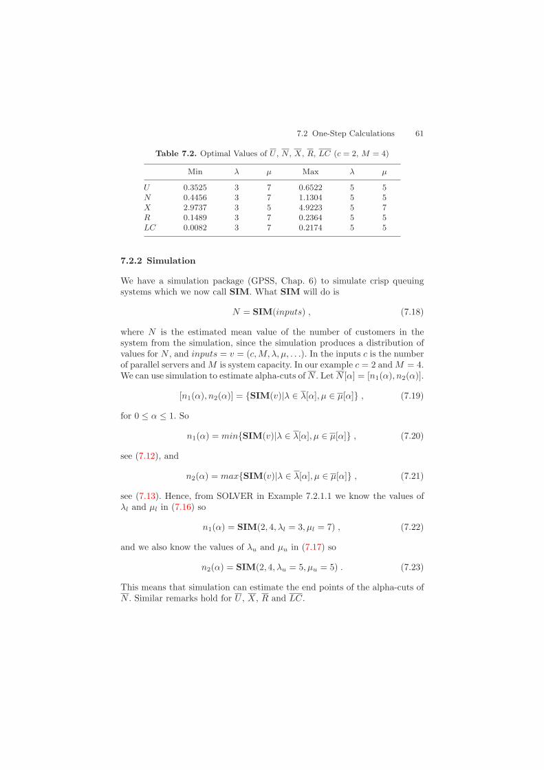
7.2 One-Step Calculations 61
Table 7.2. Optimal Values of U , N , X, R, LC (c = 2, M = 4)
Min λ µ Max λ µ
U 0.3525 3 7 0.6522 5 5N 0.4456 3 7 1.1304 5 5X 2.9737 3 5 4.9223 5 7R 0.1489 3 7 0.2364 5 5LC 0.0082 3 7 0.2174 5 5
7.2.2 Simulation
We have a simulation package (GPSS, Chap. 6) to simulate crisp queuingsystems which we now call SIM. What SIM will do is
N = SIM(inputs) , (7.18)
where N is the estimated mean value of the number of customers in thesystem from the simulation, since the simulation produces a distribution ofvalues for N , and inputs = v = (c,M, λ, µ, . . .). In the inputs c is the numberof parallel servers and M is system capacity. In our example c = 2 and M = 4.We can use simulation to estimate alpha-cuts of N . Let N [α] = [n1(α), n2(α)].
[n1(α), n2(α)] = SIM(v)|λ ∈ λ[α], µ ∈ µ[α] , (7.19)
for 0 ≤ α ≤ 1. So
n1(α) = minSIM(v)|λ ∈ λ[α], µ ∈ µ[α] , (7.20)
see (7.12), and
n2(α) = maxSIM(v)|λ ∈ λ[α], µ ∈ µ[α] , (7.21)
see (7.13). Hence, from SOLVER in Example 7.2.1.1 we know the values ofλl and µl in (7.16) so
n1(α) = SIM(2, 4, λl = 3, µl = 7) , (7.22)
and we also know the values of λu and µu in (7.17) so
n2(α) = SIM(2, 4, λu = 5, µu = 5) . (7.23)
This means that simulation can estimate the end points of the alpha-cuts ofN . Similar remarks hold for U , X, R and LC.

62 7 Queuing I: One-Step Calculations
Example 7.2.2.1
This continues Example 7.2.1.1. We used GPSS/H. The simulation programwas
1. SIMULATE2. REAL &C(1),&D(1),&E(1),&F(1)3. OUT FILEDEF ’ANS.OUT’4. STORAGE S(WORK),25. STORAGE S(BUFFER),26. GENERATE RVEXPO(1,0.3333)7. TEST LE S(BUFFER),1,POUT28. QUEUE SYSTQ9. TEST E S(WORK),0,JUMP1
10. BLET &D(1)=&D(1)+111. TRANSFER ,NEXT12. JUMP1 TEST E S(WORK),1,JUMP213. BLET &F(1)=&F(1)+114. TRANSFER ,NEXT15. JUMP2 TEST E S(WORK),2,NEXT16. BLET &C(1)=&C(1)+117. NEXT ENTER BUFFER18. ADVANCE19. ENTER WORK20. LEAVE BUFFER21. ADVANCE RVEXPO(1,0.1428)22. LEAVE WORK23. DEPART SYSTQ24. TRANSFER ,POUT125. POUT2 BLET &E(1)=&E(1)+126. TERMINATE 127. POUT1 TERMINATE 128. START 500,00029. PUTPIC FILE=OUT,LINES=8,(&C(1),&F(1),&D(1),&E(1))
NUMBER FULL ****NUMBER ONE ****NUMBER EMPTY ****NUMBER LOST ****
30. END
A brief explanation of this program is needed. The command “SIMU-LATE” starts it off and then we define &C(1),&D(1),&E(1) and &F(1) tobe a real numbers. &C(1) will count the number of times the servers areboth busy, &D(1) counts the number of times both servers are idle, &E(1)counts the number of lost customers due to the system at capacity and &F(1)counts the number of times only one server is busy. The next line defines a

7.2 One-Step Calculations 63
file “OUT” which will contain the final value of &C(1),&D(1),&E(1) and&F(1). Two storage items are defined next: (1) WORK will contain the twoidentical and parallel servers; and (2) BUFFER will be the queue in front ofWORK with capacity two customers. GENERATE makes arrivals accordingto the exponential distribution, using random number stream number one,with mean 0.3333 time units between arrivals. The TEST statement sees ifthe system is at capacity (4), and if it is the customer is sent to POUT2,counted as a lost customer and TERMINATED. QUEUE SYSQ, and laterDEPART SYSQ, allows for statistics (time in the system, . . .) to be gath-ered on the system. Then we have a series of tests to update the values of&C(1),&D(1) and &F(1). The customer then enters BUFFER if the serversare busy and ADVANCE, all by itself, says there is no delay to be expe-rienced within BUFFER except to wait for a free server. When a server isfree a customer can enter WORK and the server time is governed by theexponential with mean 0.1428. Finally, after WORK, the customer goes toPOUT1 and leaves the system. The file OUT will contain the number oftimes the system was empty when a new customer arrived, the total numberof lost customers, etc. The rest of the statistics we want will be containedin the standard output report compiled by GPSS/H. The author does notclaim that these GPSS programs are the most efficient since he learned thelanguage while writing this book.
We ran the program until 500,000 customers arrived at the system. Runtime would be expected to be less than 5 seconds. There are two commonmethods of handling “steady-state” statistics [1]: (1) “swamping”; and (2)“deletion”. In the exact one-step calculations we assumed that we were insteady-state. Initially at start-up, the system has some transient behavior,due to it beginning empty, and as time goes on the transient behavior diesdown and we proceed into steady-state. In the “swamping” method we sim-ulate for a long period so that the effect of the initial conditions becomesinsignificant. This is what we did with a simulation of 500,000 customers. Inthe “deletion” method we would break the simulation down into two parts,an initial warm up phase, followed by a data collection period. We will usethe swamping method throughout the book.
The results of the simulation, using the optimal values of λ and µ fromTable 7.2, are shown in Table 7.3. All of these values are very close to thosein Table 7.2.
In the standard output report from GPSS/H we find N and R underQUEUE. To estimate p0 we compute &D(1)/500,000 and then 1 − p0 is U .Some customers are lost due to maximum capacity of 4, but the standardoutput report contains CLOCK = the total number of elapsed time unitsfor the 500,000 simulation run. Then 500,000−&E(1) = the total number ofcustomers who left the system after passing through a server. Hence, X is esti-mated by [500,000−&E(1)]/CLOCK. LC is estimated by &E(1)/CLOCK.
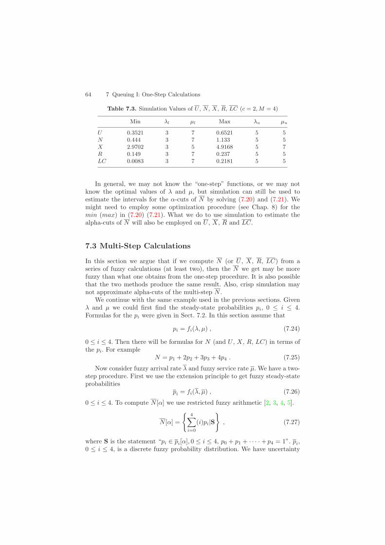
64 7 Queuing I: One-Step Calculations
Table 7.3. Simulation Values of U , N , X, R, LC (c = 2, M = 4)
Min λl µl Max λu µu
U 0.3521 3 7 0.6521 5 5N 0.444 3 7 1.133 5 5X 2.9702 3 5 4.9168 5 7R 0.149 3 7 0.237 5 5LC 0.0083 3 7 0.2181 5 5
In general, we may not know the “one-step” functions, or we may notknow the optimal values of λ and µ, but simulation can still be used toestimate the intervals for the α-cuts of N by solving (7.20) and (7.21). Wemight need to employ some optimization procedure (see Chap. 8) for themin (max) in (7.20) (7.21). What we do to use simulation to estimate thealpha-cuts of N will also be employed on U , X, R and LC.
7.3 Multi-Step Calculations
In this section we argue that if we compute N (or U , X, R, LC) from aseries of fuzzy calculations (at least two), then the N we get may be morefuzzy than what one obtains from the one-step procedure. It is also possiblethat the two methods produce the same result. Also, crisp simulation maynot approximate alpha-cuts of the multi-step N .
We continue with the same example used in the previous sections. Givenλ and µ we could first find the steady-state probabilities pi, 0 ≤ i ≤ 4.Formulas for the pi were given in Sect. 7.2. In this section assume that
pi = fi(λ, µ) , (7.24)
0 ≤ i ≤ 4. Then there will be formulas for N (and U , X, R, LC) in terms ofthe pi. For example
N = p1 + 2p2 + 3p3 + 4p4 . (7.25)
Now consider fuzzy arrival rate λ and fuzzy service rate µ. We have a two-step procedure. First we use the extension principle to get fuzzy steady-stateprobabilities
pi = fi(λ, µ) , (7.26)
0 ≤ i ≤ 4. To compute N [α] we use restricted fuzzy arithmetic [2, 3, 4, 5].
N [α] =
4∑
i=0
(i)pi|S
, (7.27)
where S is the statement “pi ∈ pi[α], 0 ≤ i ≤ 4, p0 + p1 + · · · · + p4 = 1”. pi,0 ≤ i ≤ 4, is a discrete fuzzy probability distribution. We have uncertainty
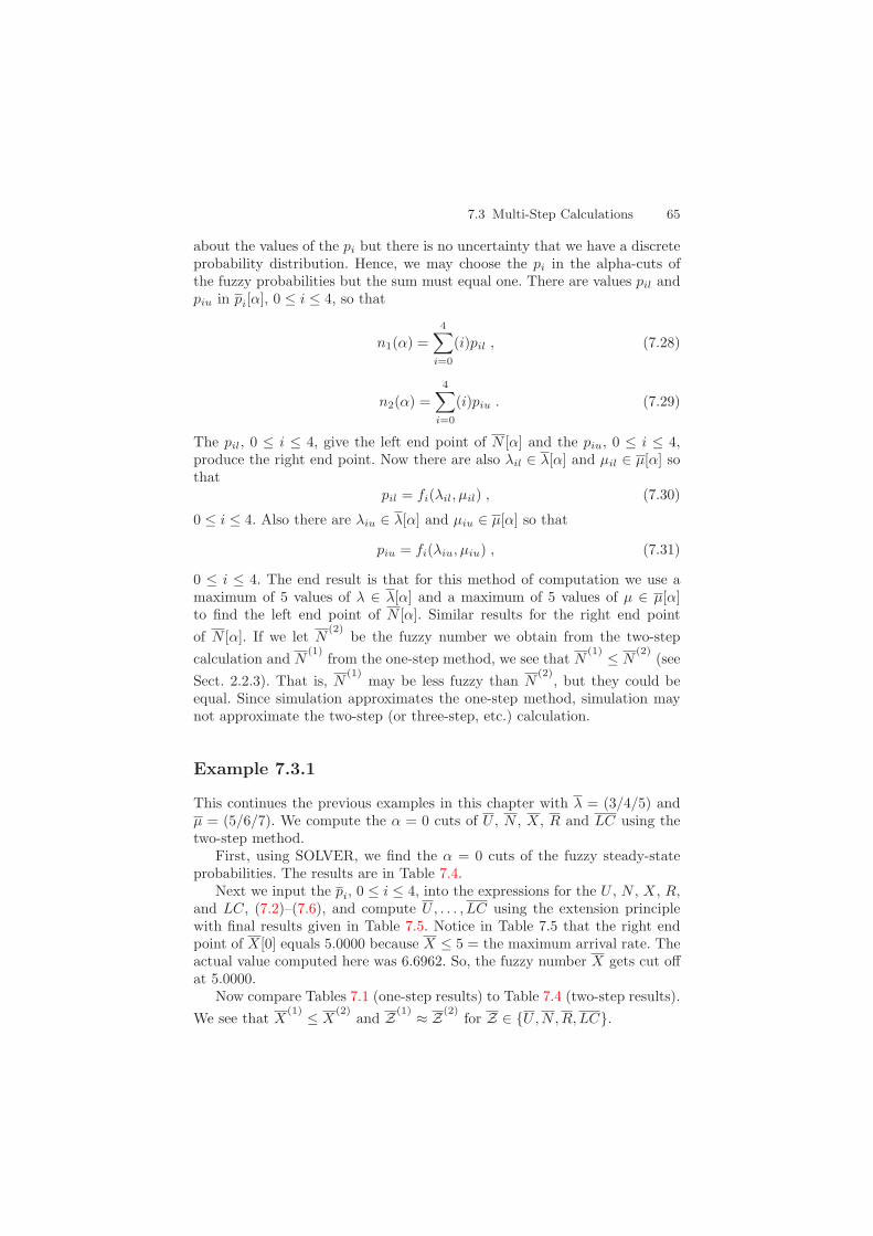
7.3 Multi-Step Calculations 65
about the values of the pi but there is no uncertainty that we have a discreteprobability distribution. Hence, we may choose the pi in the alpha-cuts ofthe fuzzy probabilities but the sum must equal one. There are values pil andpiu in pi[α], 0 ≤ i ≤ 4, so that
n1(α) =4∑
i=0
(i)pil , (7.28)
n2(α) =4∑
i=0
(i)piu . (7.29)
The pil, 0 ≤ i ≤ 4, give the left end point of N [α] and the piu, 0 ≤ i ≤ 4,produce the right end point. Now there are also λil ∈ λ[α] and µil ∈ µ[α] sothat
pil = fi(λil, µil) , (7.30)
0 ≤ i ≤ 4. Also there are λiu ∈ λ[α] and µiu ∈ µ[α] so that
piu = fi(λiu, µiu) , (7.31)
0 ≤ i ≤ 4. The end result is that for this method of computation we use amaximum of 5 values of λ ∈ λ[α] and a maximum of 5 values of µ ∈ µ[α]to find the left end point of N [α]. Similar results for the right end pointof N [α]. If we let N
(2)be the fuzzy number we obtain from the two-step
calculation and N(1)
from the one-step method, we see that N(1) ≤ N
(2)(see
Sect. 2.2.3). That is, N(1)
may be less fuzzy than N(2)
, but they could beequal. Since simulation approximates the one-step method, simulation maynot approximate the two-step (or three-step, etc.) calculation.
Example 7.3.1
This continues the previous examples in this chapter with λ = (3/4/5) andµ = (5/6/7). We compute the α = 0 cuts of U , N , X, R and LC using thetwo-step method.
First, using SOLVER, we find the α = 0 cuts of the fuzzy steady-stateprobabilities. The results are in Table 7.4.
Next we input the pi, 0 ≤ i ≤ 4, into the expressions for the U , N , X, R,and LC, (7.2)–(7.6), and compute U, . . . , LC using the extension principlewith final results given in Table 7.5. Notice in Table 7.5 that the right endpoint of X[0] equals 5.0000 because X ≤ 5 = the maximum arrival rate. Theactual value computed here was 6.6962. So, the fuzzy number X gets cut offat 5.0000.
Now compare Tables 7.1 (one-step results) to Table 7.4 (two-step results).We see that X
(1) ≤ X(2)
and Z(1) ≈ Z(2)for Z ∈ U,N,R,LC.

66 7 Queuing I: One-Step Calculations
Table 7.4. Alpha Cuts of the Fuzzy Probabilities in Example 7.3.1 (c = 2, M = 4)
Alpha = Zero Cut Alpha = One Cut
p0 [0.3478, 0.6475] 0.5031p1 [0.2775, 0.3503] 0.3354p2 [0.0595, 0.1739] 0.1118p3 [0.0127, 0.0870] 0.0373p4 [0.0027, 0.0435] 0.0124
Table 7.5. Two-Step Alpha Cuts of U , N , X, R, LC in Example 7.3.1(c = 2, M = 4)
Alpha = Zero Cut Alpha = One Cut
U [0.3525, 0.6522] 0.4969
N [0.4455, 1.1306] 0.7205
X [2.1370, 5.0000] 3.9504
R [0.1464, 0.2529] 0.1824
LC [0.0081, 0.2175] 0.0497
Example 7.3.1 shows that in using two-step fuzzy calculations sometimeswe get the same result as in the one-step calculation and we may get adifferent (more fuzzy) answer. In the rest of the book we will want to computemany other fuzzy numbers besides those for U , N , X, R and LC. We willusually not know, for all these fuzzy numbers, if the one-step and the multi-step fuzzy calculations agree. So, to be on the “safe side” we will only usesimulation to approximate the α-cuts of the fuzzy numbers obtained fromone-step calculations.
7.4 Rest of the Book
In the applications in the following chapters, Chaps. 9–26, we will use simu-lation to approximate alpha-cuts of certain fuzzy system descriptors like N ,U , X, R and LC when we do not have a one-step calculation available. Thesesystems will be sufficiently complicated so that a one-step expression for N ,U , X, R and LC is too difficult to derive and we do not know how to findit in the literature. We assume a continuous one-step function theoreticallyexists, but in practice we do not know a formula for this function, and thesimulation approximates the results of this (unknown) one-step calculation.The way to analyze these fuzzy systems is through simulation.
All of these systems use probabilities and probability distributions. Wemust estimate these probabilities, or the parameters in the distributions,from crisp data. Our estimators will all be fuzzy estimators (Chap. 3). Fuzzy

References 67
estimators force the system to become a fuzzy system whose analysis is ac-complished by computing fuzzy numbers for N , U , X, R, etc. All these fuzzycalculations will be approximated by simulation.
References
1. J. Banks, J.S. Carson and J.N. Sy: Getting Started with GPSS/H, Second Edi-tion, Wolverine Software Corp., Annandale, VA, 1995.
2. J.J. Buckley: Fuzzy Probabilities: New Approach and Applications,Physica-Verlag, Heidelberg, Germany, 2003. 64
3. J.J. Buckley: Fuzzy Probabilities and Fuzzy Sets for Web Planning, Springer,Heidelberg, Germany, 2004. 64
4. J.J. Buckley and E. Eslami: Uncertain Probabilities I: The Discrete Case, SoftComputing, 7(2003)500-505. 64
5. J.J. Buckley, K. Reilly and X. Zheng: Fuzzy Probabilities for Web Planning,Soft Computing, 8(2004)464-476. 64
6. J.J. Buckley: Maximum Entropy Principle with Imprecise Side-Conditions II:Crisp Discrete Solutions, Soft Computing. To appear.
7. Frontline Systems (www.frontsys.com, www.solver.com).8. H.A. Taha: Operations Research, Fifth Edition, Macmillan, N.Y., 1992. 57

8 Simulation Optimization
8.1 Introduction
In this chapter we discuss how we plan to solve the optimization problemsattached to the simulation as expressed in (5.4)–(5.5) in Chap. 5, or (7.20)–(7.21) in Chap. 7, without the use of a one-step function. Consider the fuzzysystem of Chap. 5, shown in Fig. 5.1, and the servers S41,S42,S43. Each ofthese servers has service time described by a normal distribution N(µ4, σ
24).
For this fuzzy system we want to compute X the fuzzy number for through-put. To approximate X we need some of its α-cuts. Now we first obtain fuzzyestimators for µ4 and σ2
4 which are µ4 and σ24, respectively. Choose α ∈ [0, 1).
The optimization problem to solve is to decide on µ ∈ µ4[α] and σ ∈ σ24[α] to
use in the simulation so that the output approximates the end points of X[α].This has to be done for all the fuzzy estimators in all the fuzzy distributionsemployed by the system.
In this book there are only three places in a fuzzy system that dependon a fuzzy distribution: (1) arrivals; (2) service stations; and (3) randomtransfer points. We now look at each of these and how we hope to solve theoptimization problem.
8.2 Arrivals
In this book all arrivals will usually be governed by the exponential distri-bution. To describe arrivals we use λ = the number of items (customers)arriving per unit time and 1/λ = the mean time between arrivals. The solu-tion to the optimization problem is given in Table 8.1. We have assumed thatall parameters in the fuzzy system are held fixed except λ for this arrival.If λ is our fuzzy estimator of λ, let [λl, λu] = [λ1(α), λ2(α)] = λ[α] for somefixed α ∈ [0, 1).
We interpret Table 8.1 as follows: (1) if we want to approximate the leftend point of the interval X[α] use for λ the left end point of the interval λ[α];and (2) if you want to approximate the right end point of the interval R usefor λ the right end point of the interval λ[α].
All of these results are rather intuitive. Let λ increase from its minimumλl to its maximum λu. All other parameters of the system are held fixed. The
James J. Buckley: Simulating Fuzzy Systems, StudFuzz 171, 69–73 (2005)www.springerlink.com c© Springer-Verlag Berlin Heidelberg 2005

70 8 Simulation Optimization
Table 8.1. Optimal Values of λ ∈ [λl, λu] = λ[α] for Fuzzy Exponential Arrivalsin Simulation
Min λ Max λ
U λl U λu
N λl N λu
R λl R λu
X λl X λu
LC λl LC λu
system becomes more congested. We will call arrivals “customers”, but theyneed not be people. More and more customers will fill the queues in front ofthe servers. This means that server utilization (mean value = U) increases,number of customers in the system (mean value = N) increases and the timea customer spends in the system (mean value = R) also increases. At firstit is not clear what happens to the number of customers leaving the systemper unit time (mean = X) since X = N/R. But the number leaving perunit time will not decrease, so X will also increase. If the system has finitecapacity, then the number of customers lost per unit time (LC) increases as λincreases. These results are what is in Table 8.1. The same results are shownin Tables 7.2 and 7.3. The units in Table 8.1 for λ are number of customersarriving per unit time and not the number of time units between arrivals.
8.3 Service
In this book we will use for the service probability distribution the: (1) ex-ponential; (2) uniform; and (3) normal.
8.3.1 Exponential
The number of service completions per unit time is µ so the mean servicetime is 1/µ. The exponential depends only on one parameter µ. The solutionto the optimization problem is given in Table 8.2. If µ is our fuzzy estimatorof µ, let [µl, µu] = [µ1(α), µ2(α)] = µ[α] for some fixed α ∈ [0, 1).
We interpret Table 8.2 as follows: (1) if we want to approximate the leftend point of the interval X[α] use for µ the left end point of the interval µ[α];and (2) if you want to approximate the right end point of the interval R usefor µ the left end point of the interval µ[α].
All of these results are also intuitive. Let µ increase from its minimum µl
to its maximum µu. All other parameters of the system are held fixed. Thisservice station may have c (c ≥ 1) parallel and identical servers. The systemconsisting of this server and what comes before it, becomes less congested.Fewer and fewer customers fill the queue in front of this server. This means
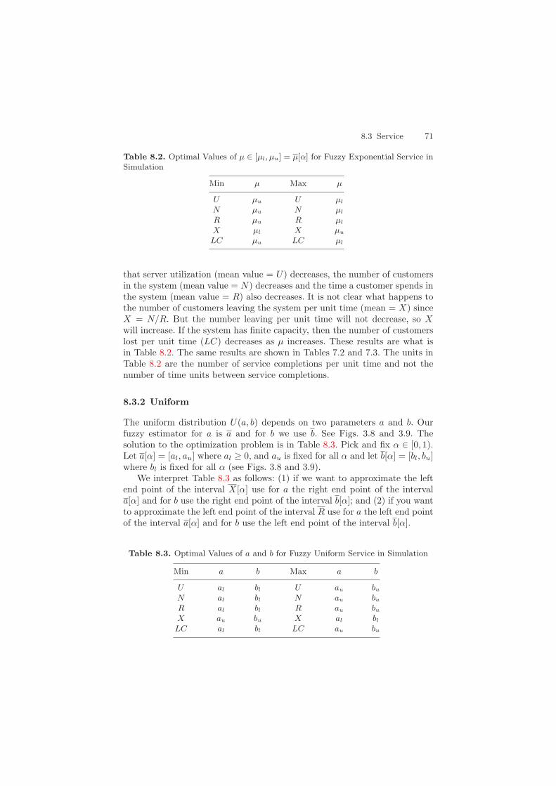
8.3 Service 71
Table 8.2. Optimal Values of µ ∈ [µl, µu] = µ[α] for Fuzzy Exponential Service inSimulation
Min µ Max µ
U µu U µl
N µu N µl
R µu R µl
X µl X µu
LC µu LC µl
that server utilization (mean value = U) decreases, the number of customersin the system (mean value = N) decreases and the time a customer spends inthe system (mean value = R) also decreases. It is not clear what happens tothe number of customers leaving the system per unit time (mean = X) sinceX = N/R. But the number leaving per unit time will not decrease, so Xwill increase. If the system has finite capacity, then the number of customerslost per unit time (LC) decreases as µ increases. These results are what isin Table 8.2. The same results are shown in Tables 7.2 and 7.3. The units inTable 8.2 are the number of service completions per unit time and not thenumber of time units between service completions.
8.3.2 Uniform
The uniform distribution U(a, b) depends on two parameters a and b. Ourfuzzy estimator for a is a and for b we use b. See Figs. 3.8 and 3.9. Thesolution to the optimization problem is in Table 8.3. Pick and fix α ∈ [0, 1).Let a[α] = [al, au] where al ≥ 0, and au is fixed for all α and let b[α] = [bl, bu]where bl is fixed for all α (see Figs. 3.8 and 3.9).
We interpret Table 8.3 as follows: (1) if we want to approximate the leftend point of the interval X[α] use for a the right end point of the intervala[α] and for b use the right end point of the interval b[α]; and (2) if you wantto approximate the left end point of the interval R use for a the left end pointof the interval a[α] and for b use the left end point of the interval b[α].
Table 8.3. Optimal Values of a and b for Fuzzy Uniform Service in Simulation
Min a b Max a b
U al bl U au bu
N al bl N au bu
R al bl R au bu
X au bu X al bl
LC al bl LC au bu

72 8 Simulation Optimization
It can be confusing to compare Tables 8.2 and 8.3. Table 8.2 uses max/minrates but Table 8.3 has max/min times. A min (max) rate corresponds to amax (min) time. The values in Table 8.3 are about times to service comple-tion.
The discussion on why Table 8.3 is correct is similar to why Table 8.2is correct. All other parameters are held fixed. Analysis of Table 8.3 centersaround the mean service time ((a + b)/2) of the uniform U(a, b). You min-imize (a + b)/2 to minimize U , N , R, LC and you maximize (a + b)/2 tomaximize U , N , R, LC. But you minimize (maximize) the mean service timeto maximize (minimize) X.
8.3.3 Normal
The normal distribution N(µ, σ2) depends on two parameters µ and σ2. Ourfuzzy estimator for µ is µ and for σ2 we use σ2. See Chap. 3. The solutionto the optimization problem is in Table 8.4. Pick and fix α ∈ [0, 1). Letµ[α] = [µl, µu].
Table 8.4. Optimal Values of µ for Fuzzy Normal Service in Simulation
Min µ Max µ
U µl U µu
N µl N µu
R µl R µu
X µu X µl
LC µl LC µu
We interpret Table 8.4 as follows: (1) if we want to approximate the leftend point of the interval X[α] use for µ the right end point of the intervalµ[α]; and (2) if you want to approximate the left end point of the interval Ruse for µ the left end point of the interval µ[α]. The values in Table 8.4 areservice times not service rates.
The discussion on why Table 8.3 is correct is similar to why Tables 8.2and 8.3 are correct. We pick and fix the values of all the other parameters.You minimize (maximize) µ to minimize (maximize) U , N , R, LC and youmaximize (minimize) µ to minimize (maximize) X.
Notice that no values of σ2 are in Table 8.4. This is because the results areapproximately independent of σ2. If you hold µ fixed and vary σ2 throughoutsome interval, remember to keep µ−5σ2 > 0, the values for U , N , X, R, LCare relatively constant. We did notice that the number of customers lost canincrease as σ2 increases, but the value of the CLOCK can also change, leavingLC was almost constant. All simulations using normal service times, show-ing independence of the variance, were done using the example in Chap. 7(Fig. 7.1).
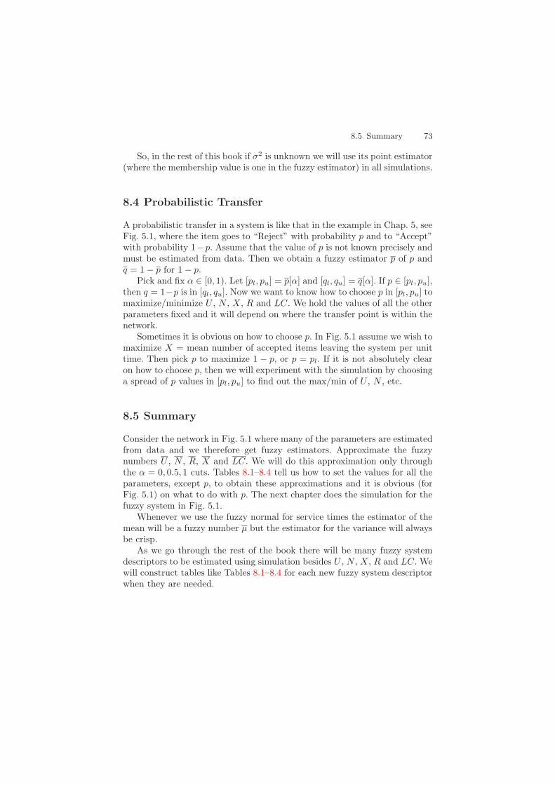
8.5 Summary 73
So, in the rest of this book if σ2 is unknown we will use its point estimator(where the membership value is one in the fuzzy estimator) in all simulations.
8.4 Probabilistic Transfer
A probabilistic transfer in a system is like that in the example in Chap. 5, seeFig. 5.1, where the item goes to “Reject” with probability p and to “Accept”with probability 1−p. Assume that the value of p is not known precisely andmust be estimated from data. Then we obtain a fuzzy estimator p of p andq = 1 − p for 1 − p.
Pick and fix α ∈ [0, 1). Let [pl, pu] = p[α] and [ql, qu] = q[α]. If p ∈ [pl, pu],then q = 1−p is in [ql, qu]. Now we want to know how to choose p in [pl, pu] tomaximize/minimize U , N , X, R and LC. We hold the values of all the otherparameters fixed and it will depend on where the transfer point is within thenetwork.
Sometimes it is obvious on how to choose p. In Fig. 5.1 assume we wish tomaximize X = mean number of accepted items leaving the system per unittime. Then pick p to maximize 1 − p, or p = pl. If it is not absolutely clearon how to choose p, then we will experiment with the simulation by choosinga spread of p values in [pl, pu] to find out the max/min of U , N , etc.
8.5 Summary
Consider the network in Fig. 5.1 where many of the parameters are estimatedfrom data and we therefore get fuzzy estimators. Approximate the fuzzynumbers U , N , R, X and LC. We will do this approximation only throughthe α = 0, 0.5, 1 cuts. Tables 8.1–8.4 tell us how to set the values for all theparameters, except p, to obtain these approximations and it is obvious (forFig. 5.1) on what to do with p. The next chapter does the simulation for thefuzzy system in Fig. 5.1.
Whenever we use the fuzzy normal for service times the estimator of themean will be a fuzzy number µ but the estimator for the variance will alwaysbe crisp.
As we go through the rest of the book there will be many fuzzy systemdescriptors to be estimated using simulation besides U , N , X, R and LC. Wewill construct tables like Tables 8.1–8.4 for each new fuzzy system descriptorwhen they are needed.
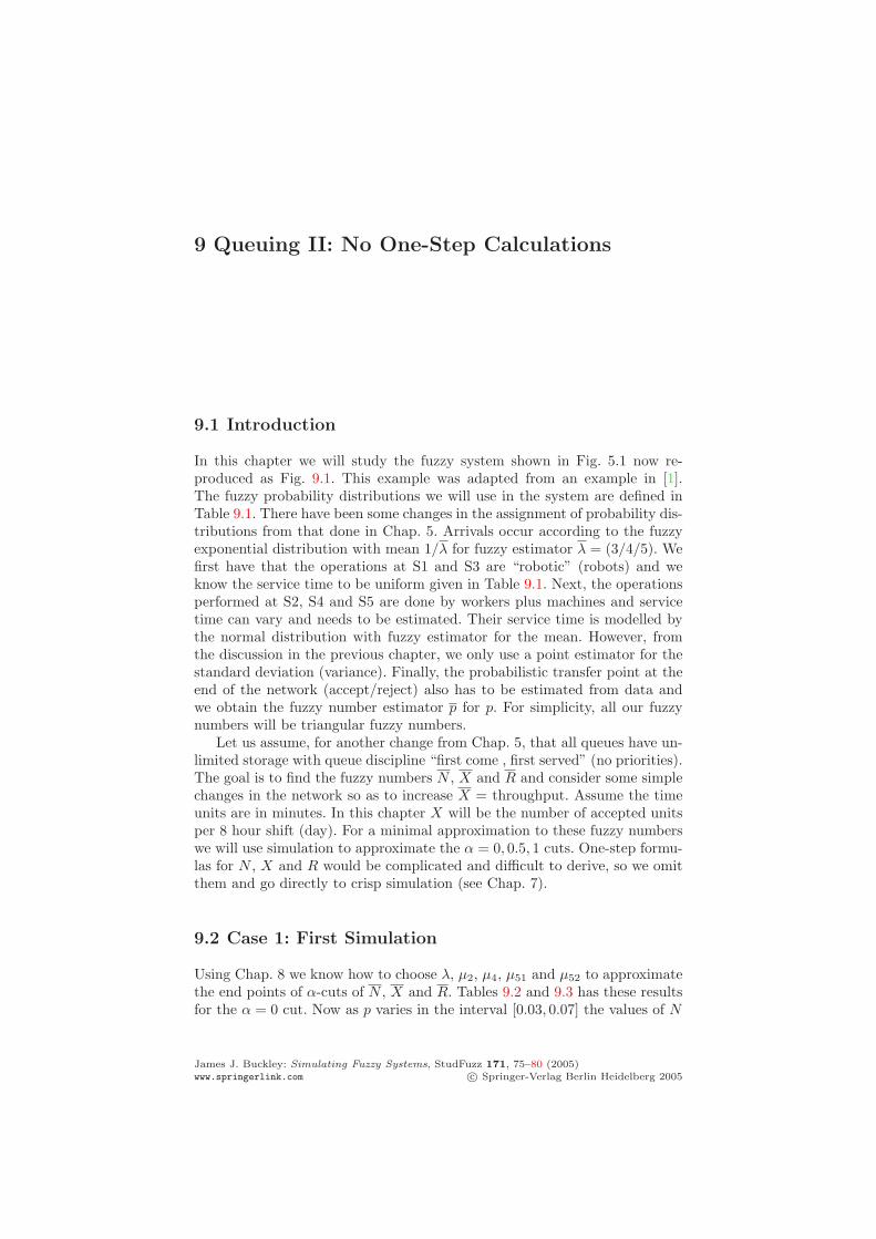
9 Queuing II: No One-Step Calculations
9.1 Introduction
In this chapter we will study the fuzzy system shown in Fig. 5.1 now re-produced as Fig. 9.1. This example was adapted from an example in [1].The fuzzy probability distributions we will use in the system are defined inTable 9.1. There have been some changes in the assignment of probability dis-tributions from that done in Chap. 5. Arrivals occur according to the fuzzyexponential distribution with mean 1/λ for fuzzy estimator λ = (3/4/5). Wefirst have that the operations at S1 and S3 are “robotic” (robots) and weknow the service time to be uniform given in Table 9.1. Next, the operationsperformed at S2, S4 and S5 are done by workers plus machines and servicetime can vary and needs to be estimated. Their service time is modelled bythe normal distribution with fuzzy estimator for the mean. However, fromthe discussion in the previous chapter, we only use a point estimator for thestandard deviation (variance). Finally, the probabilistic transfer point at theend of the network (accept/reject) also has to be estimated from data andwe obtain the fuzzy number estimator p for p. For simplicity, all our fuzzynumbers will be triangular fuzzy numbers.
Let us assume, for another change from Chap. 5, that all queues have un-limited storage with queue discipline “first come , first served” (no priorities).The goal is to find the fuzzy numbers N , X and R and consider some simplechanges in the network so as to increase X = throughput. Assume the timeunits are in minutes. In this chapter X will be the number of accepted unitsper 8 hour shift (day). For a minimal approximation to these fuzzy numberswe will use simulation to approximate the α = 0, 0.5, 1 cuts. One-step formu-las for N , X and R would be complicated and difficult to derive, so we omitthem and go directly to crisp simulation (see Chap. 7).
9.2 Case 1: First Simulation
Using Chap. 8 we know how to choose λ, µ2, µ4, µ51 and µ52 to approximatethe end points of α-cuts of N , X and R. Tables 9.2 and 9.3 has these resultsfor the α = 0 cut. Now as p varies in the interval [0.03, 0.07] the values of N
James J. Buckley: Simulating Fuzzy Systems, StudFuzz 171, 75–80 (2005)www.springerlink.com c© Springer-Verlag Berlin Heidelberg 2005
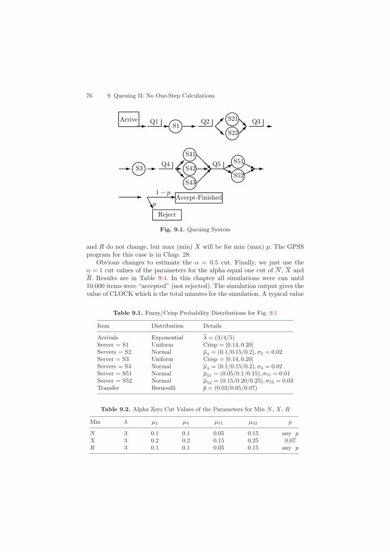
76 9 Queuing II: No One-Step Calculations
Arrive Q1
S1 Q2
S21
S22
Q3
S3 Q4
S41
S42
S43
Q5
S51
S52
Accept-Finished
Reject
1 − p
p
Fig. 9.1. Queuing System
and R do not change, but max (min) X will be for min (max) p. The GPSSprogram for this case is in Chap. 28.
Obvious changes to estimate the α = 0.5 cut. Finally, we just use theα = 1 cut values of the parameters for the alpha equal one cut of N , X andR. Results are in Table 9.4. In this chapter all simulations were run until10,000 items were “accepted” (not rejected). The simulation output gives thevalue of CLOCK which is the total minutes for the simulation. A typical value
Table 9.1. Fuzzy/Crisp Probability Distributions for Fig. 9.1
Item Distribution Details
Arrivals Exponential λ = (3/4/5)Server = S1 Uniform Crisp = [0.14, 0.20]Servers = S2 Normal µ2 = (0.1/0.15/0.2), σ2 = 0.02Server = S3 Uniform Crisp = [0.14, 0.20]Servers = S4 Normal µ4 = (0.1/0.15/0.2), σ4 = 0.02Server = S51 Normal µ51 = (0.05/0.1/0.15), σ51 = 0.01Server = S52 Normal µ52 = (0.15/0.20/0.25), σ52 = 0.03Transfer Bernoulli p = (0.03/0.05/0.07)
Table 9.2. Alpha Zero Cut Values of the Parameters for Min N , X, R
Min λ µ2 µ4 µ51 µ52 p
N 3 0.1 0.1 0.05 0.15 any pX 3 0.2 0.2 0.15 0.25 0.07R 3 0.1 0.1 0.05 0.15 any p
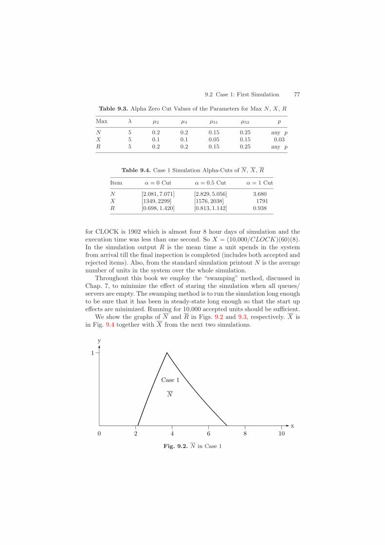
9.2 Case 1: First Simulation 77
Table 9.3. Alpha Zero Cut Values of the Parameters for Max N , X, R
Max λ µ2 µ4 µ51 µ52 p
N 5 0.2 0.2 0.15 0.25 any pX 5 0.1 0.1 0.05 0.15 0.03R 5 0.2 0.2 0.15 0.25 any p
Table 9.4. Case 1 Simulation Alpha-Cuts of N , X, R
Item α = 0 Cut α = 0.5 Cut α = 1 Cut
N [2.081, 7.071] [2.829, 5.056] 3.680X [1349, 2299] [1576, 2038] 1791R [0.698, 1.420] [0.813, 1.142] 0.938
for CLOCK is 1902 which is almost four 8 hour days of simulation and theexecution time was less than one second. So X = (10,000/CLOCK)(60)(8).In the simulation output R is the mean time a unit spends in the systemfrom arrival till the final inspection is completed (includes both accepted andrejected items). Also, from the standard simulation printout N is the averagenumber of units in the system over the whole simulation.
Throughout this book we employ the “swamping” method, discussed inChap. 7, to minimize the effect of staring the simulation when all queues/servers are empty. The swamping method is to run the simulation long enoughto be sure that it has been in steady-state long enough so that the start upeffects are minimized. Running for 10,000 accepted units should be sufficient.
We show the graphs of N and R in Figs. 9.2 and 9.3, respectively. X isin Fig. 9.4 together with X from the next two simulations.
0 2 4 6 8 10x
1
y
Case 1
N
Fig. 9.2. N in Case 1
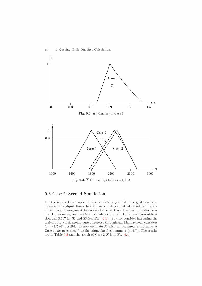
78 9 Queuing II: No One-Step Calculations
0 0.3 0.6 0.9 1.2 1.5x
1
y
Case 1
R
Fig. 9.3. R (Minutes) in Case 1
1000 1400 1800 2200 2600 3000x
1
0.8
y
Case 1
Case 2
Case 3
Fig. 9.4. X (Units/Day) for Cases 1, 2, 3
9.3 Case 2: Second Simulation
For the rest of this chapter we concentrate only on X. The goal now is toincrease throughput. From the standard simulation output report (not repro-duced here) management has noticed that in Case 1 server utilization waslow. For example, for the Case 1 simulation for α = 1 the maximum utiliza-tion was 0.667 for S1 and S3 (see Fig. (9.1)). So they consider increasing thearrival rate which should surely increase throughput. Management considersλ = (4/5/6) possible, so now estimate X with all parameters the same asCase 1 except change λ to the triangular fuzzy number (4/5/6). The resultsare in Table 9.5 and the graph of Case 2 X is in Fig. 9.4.
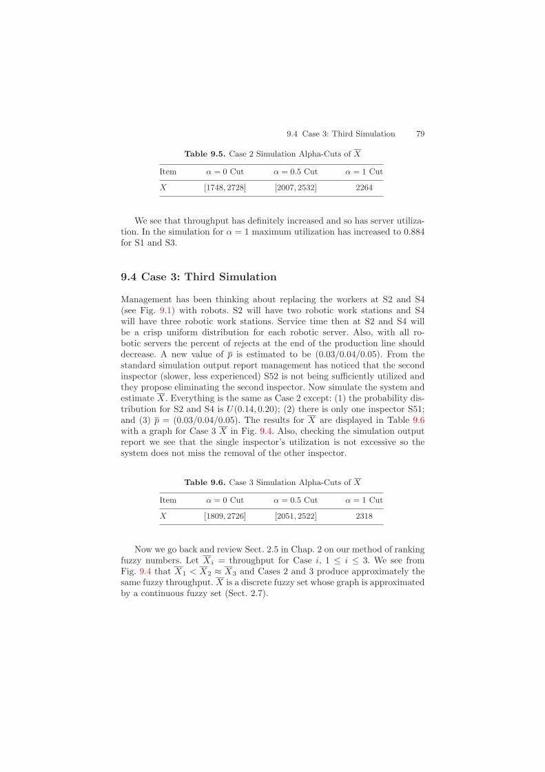
9.4 Case 3: Third Simulation 79
Table 9.5. Case 2 Simulation Alpha-Cuts of X
Item α = 0 Cut α = 0.5 Cut α = 1 Cut
X [1748, 2728] [2007, 2532] 2264
We see that throughput has definitely increased and so has server utiliza-tion. In the simulation for α = 1 maximum utilization has increased to 0.884for S1 and S3.
9.4 Case 3: Third Simulation
Management has been thinking about replacing the workers at S2 and S4(see Fig. 9.1) with robots. S2 will have two robotic work stations and S4will have three robotic work stations. Service time then at S2 and S4 willbe a crisp uniform distribution for each robotic server. Also, with all ro-botic servers the percent of rejects at the end of the production line shoulddecrease. A new value of p is estimated to be (0.03/0.04/0.05). From thestandard simulation output report management has noticed that the secondinspector (slower, less experienced) S52 is not being sufficiently utilized andthey propose eliminating the second inspector. Now simulate the system andestimate X. Everything is the same as Case 2 except: (1) the probability dis-tribution for S2 and S4 is U(0.14, 0.20); (2) there is only one inspector S51;and (3) p = (0.03/0.04/0.05). The results for X are displayed in Table 9.6with a graph for Case 3 X in Fig. 9.4. Also, checking the simulation outputreport we see that the single inspector’s utilization is not excessive so thesystem does not miss the removal of the other inspector.
Table 9.6. Case 3 Simulation Alpha-Cuts of X
Item α = 0 Cut α = 0.5 Cut α = 1 Cut
X [1809, 2726] [2051, 2522] 2318
Now we go back and review Sect. 2.5 in Chap. 2 on our method of rankingfuzzy numbers. Let Xi = throughput for Case i, 1 ≤ i ≤ 3. We see fromFig. 9.4 that X1 < X2 ≈ X3 and Cases 2 and 3 produce approximately thesame fuzzy throughput. X is a discrete fuzzy set whose graph is approximatedby a continuous fuzzy set (Sect. 2.7).
80 9 Queuing II: No One-Step Calculations
9.5 Summary
Management may go on with “what ifing” to increase X. What if we addthis? What if we change that? But we shall stop here. We used crisp sim-ulation to approximate the one-step fuzzy numbers for N , X and R. Thesefuzzy numbers incorporate the uncertainty in the data and their bases arelike a 99% confidence interval. We introduced the beginning of fuzzy systemoptimization. As you vary the fuzzy system you compute approximations tothe fuzzy numbers describing performance and then you choose the configu-ration to possibly maximize throughput and/or minimize response time. SeeSect. 2.6 of Chap. 2. We will continue to add some optimization concepts inthe following chapters.
Reference
1. J. Banks, J.S. Carson and J.N. Sy: Getting Started with GPSS/H, Second Edi-tion, Wolverine Software Corp. Annandale, VA, 1995. 75
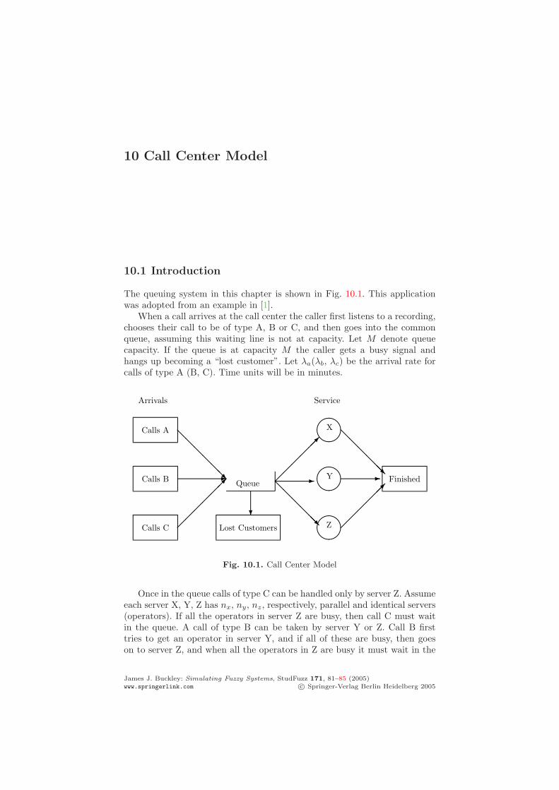
10 Call Center Model
10.1 Introduction
The queuing system in this chapter is shown in Fig. 10.1. This applicationwas adopted from an example in [1].
When a call arrives at the call center the caller first listens to a recording,chooses their call to be of type A, B or C, and then goes into the commonqueue, assuming this waiting line is not at capacity. Let M denote queuecapacity. If the queue is at capacity M the caller gets a busy signal andhangs up becoming a “lost customer”. Let λa(λb, λc) be the arrival rate forcalls of type A (B, C). Time units will be in minutes.
Calls C
Calls B
Calls A
Lost Customers
Arrivals
Queue
X
Y
Z
Service
Finished
Fig. 10.1. Call Center Model
Once in the queue calls of type C can be handled only by server Z. Assumeeach server X, Y, Z has nx, ny, nz, respectively, parallel and identical servers(operators). If all the operators in server Z are busy, then call C must waitin the queue. A call of type B can be taken by server Y or Z. Call B firsttries to get an operator in server Y, and if all of these are busy, then goeson to server Z, and when all the operators in Z are busy it must wait in the
James J. Buckley: Simulating Fuzzy Systems, StudFuzz 171, 81–85 (2005)www.springerlink.com c© Springer-Verlag Berlin Heidelberg 2005
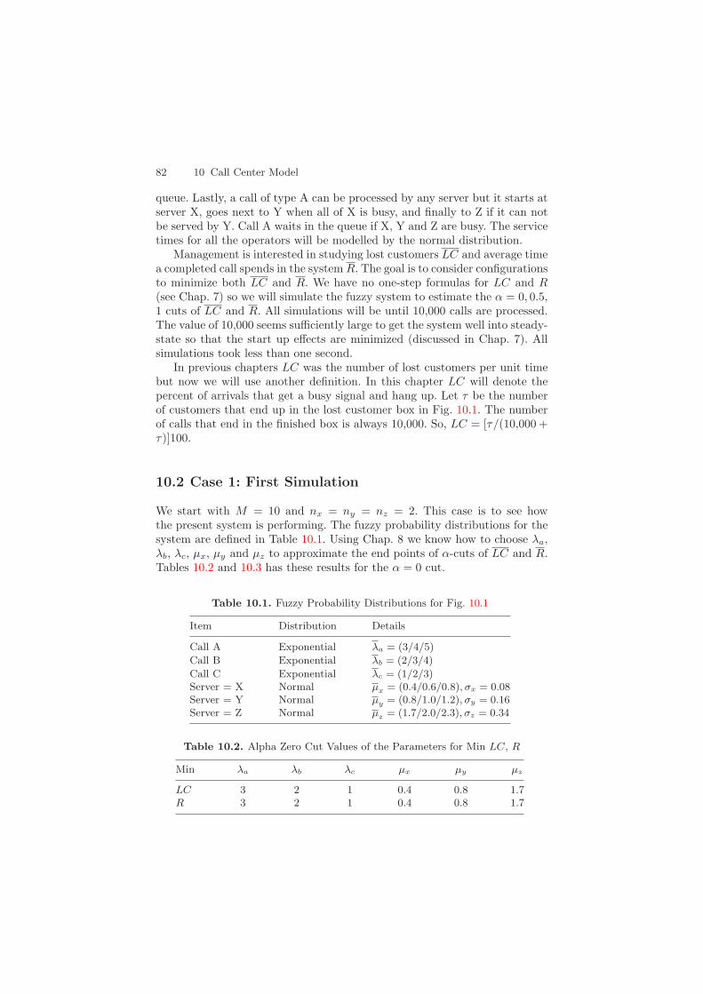
82 10 Call Center Model
queue. Lastly, a call of type A can be processed by any server but it starts atserver X, goes next to Y when all of X is busy, and finally to Z if it can notbe served by Y. Call A waits in the queue if X, Y and Z are busy. The servicetimes for all the operators will be modelled by the normal distribution.
Management is interested in studying lost customers LC and average timea completed call spends in the system R. The goal is to consider configurationsto minimize both LC and R. We have no one-step formulas for LC and R(see Chap. 7) so we will simulate the fuzzy system to estimate the α = 0, 0.5,1 cuts of LC and R. All simulations will be until 10,000 calls are processed.The value of 10,000 seems sufficiently large to get the system well into steady-state so that the start up effects are minimized (discussed in Chap. 7). Allsimulations took less than one second.
In previous chapters LC was the number of lost customers per unit timebut now we will use another definition. In this chapter LC will denote thepercent of arrivals that get a busy signal and hang up. Let τ be the numberof customers that end up in the lost customer box in Fig. 10.1. The numberof calls that end in the finished box is always 10,000. So, LC = [τ/(10,000 +τ)]100.
10.2 Case 1: First Simulation
We start with M = 10 and nx = ny = nz = 2. This case is to see howthe present system is performing. The fuzzy probability distributions for thesystem are defined in Table 10.1. Using Chap. 8 we know how to choose λa,λb, λc, µx, µy and µz to approximate the end points of α-cuts of LC and R.Tables 10.2 and 10.3 has these results for the α = 0 cut.
Table 10.1. Fuzzy Probability Distributions for Fig. 10.1
Item Distribution Details
Call A Exponential λa = (3/4/5)
Call B Exponential λb = (2/3/4)
Call C Exponential λc = (1/2/3)Server = X Normal µx = (0.4/0.6/0.8), σx = 0.08Server = Y Normal µy = (0.8/1.0/1.2), σy = 0.16Server = Z Normal µz = (1.7/2.0/2.3), σz = 0.34
Table 10.2. Alpha Zero Cut Values of the Parameters for Min LC, R
Min λa λb λc µx µy µz
LC 3 2 1 0.4 0.8 1.7R 3 2 1 0.4 0.8 1.7

10.3 Case 2: Second Simulation 83
Table 10.3. Alpha Zero Cut Values of the Parameters for Max LC, R
Max λa λb λc µx µy µz
LC 5 4 3 0.8 1.2 2.3R 5 4 3 0.8 1.2 2.3
Obvious changes to estimate the α = 0.5 cut. Finally, we just use theα = 1 cut values of the parameters for the alpha equal one cut of LC and R.Results are in Table 10.4. A typical value for CLOCK was 1520.77 which isaround three days (8 hours per day) of simulation which took less than onesecond.
Table 10.4. Case 1 Simulation Alpha-Cuts of LC, R
Item α = 0 Cut α = 0.5 Cut α = 1 Cut
LC [36, 82] [58, 77] 69R [3.242, 5.950] [4.100, 5.389] 4.726
We show the graphs of LC and R in Figs. 10.2 and 10.3, respectively.Their graphs from the other cases, discussed below, are also in these figures.
10.3 Case 2: Second Simulation
The percent of lost calls is very high and management’s goal is to reduceit. From the standard simulation output file we notice that the utilization of
0 20 40 60 80 100x
1
0.8
y
Case 3
Case 1
Case 2
Fig. 10.2. LC (Percent) in Cases 1, 2, 3

84 10 Call Center Model
1 2 3 4 5 6x
1
0.8
y
Case 1
Case 2Case 3
Fig. 10.3. R (Minutes) in Cases 1, 2, 3
the operators in server Z is 100%. This is one of the problems causing thehigh loss of calls. Server Z being too busy sends too many calls of type C tothe queue filling it to capacity. Management considers a training program forthe operators in server Y so they can also handle calls of type C. The onlychange from the system in Case 1 is that calls C first go to server Y, and if it isbusy, they are sent to server Z. Also, in Table 10.1, µy = µz = (1.7/2.0/2.3),σy = σz = 0.34. Simulation results for the α = 0, 0.5, 1 cuts of LC and R arein Table 10.5. The graphs are also shown in Figs. 10.2 and 10.3.
Table 10.5. Case 2 Simulation Alpha-Cuts of LC, R
Item α = 0 Cut α = 0.5 Cut α = 1 Cut
LC [43, 81] [60, 77] 71R [3.849, 6.199] [4.567, 5.756] 5.217
10.4 Case 3: Third Simulation
The plan for Case 2 turned out to be a disaster. In fact, from Fig. 10.2 LC evenincreased a small amount in Case 2 over Case 1. Again, from the standardsimulation output file the operators in server Z are still at 100% utilization.Management now considers: (1) adding a trained operator to server Y; (2)adding trained operators to server Z; and (3) increasing the capacity of thequeue. Top management’s goal is to get lost customers to around 20% andreduce time in the system to about 4 minutes. An average of 4 minutes inthe system allows for around 2 minutes holding time in the queue where thecaller will hear company advertisements. Everything remains the same as in
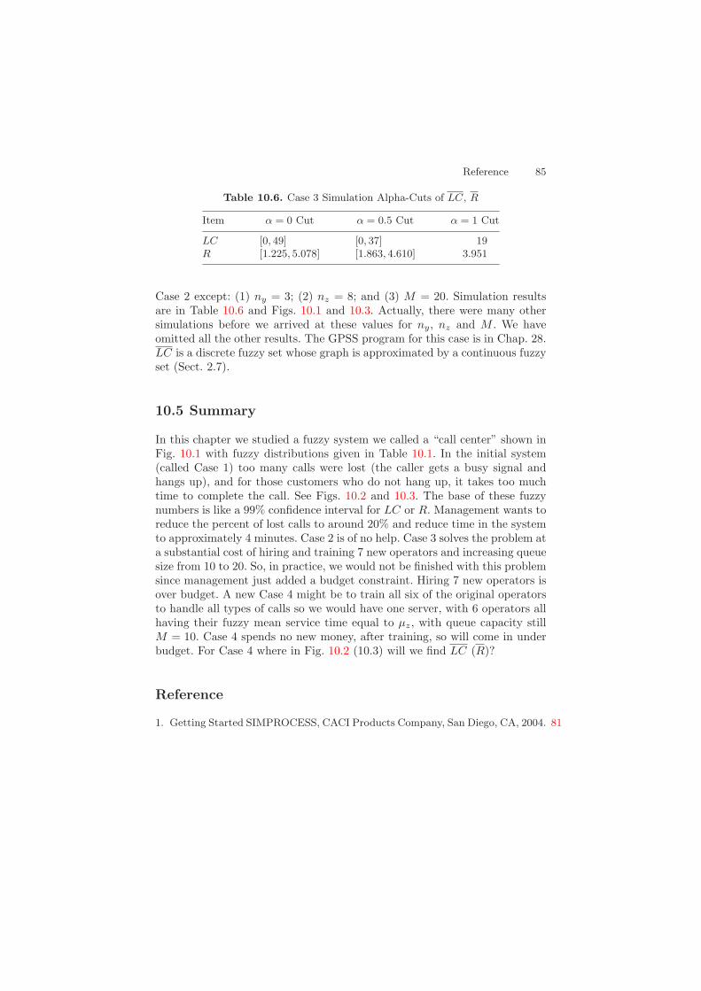
Reference 85
Table 10.6. Case 3 Simulation Alpha-Cuts of LC, R
Item α = 0 Cut α = 0.5 Cut α = 1 Cut
LC [0, 49] [0, 37] 19R [1.225, 5.078] [1.863, 4.610] 3.951
Case 2 except: (1) ny = 3; (2) nz = 8; and (3) M = 20. Simulation resultsare in Table 10.6 and Figs. 10.1 and 10.3. Actually, there were many othersimulations before we arrived at these values for ny, nz and M . We haveomitted all the other results. The GPSS program for this case is in Chap. 28.LC is a discrete fuzzy set whose graph is approximated by a continuous fuzzyset (Sect. 2.7).
10.5 Summary
In this chapter we studied a fuzzy system we called a “call center” shown inFig. 10.1 with fuzzy distributions given in Table 10.1. In the initial system(called Case 1) too many calls were lost (the caller gets a busy signal andhangs up), and for those customers who do not hang up, it takes too muchtime to complete the call. See Figs. 10.2 and 10.3. The base of these fuzzynumbers is like a 99% confidence interval for LC or R. Management wants toreduce the percent of lost calls to around 20% and reduce time in the systemto approximately 4 minutes. Case 2 is of no help. Case 3 solves the problem ata substantial cost of hiring and training 7 new operators and increasing queuesize from 10 to 20. So, in practice, we would not be finished with this problemsince management just added a budget constraint. Hiring 7 new operators isover budget. A new Case 4 might be to train all six of the original operatorsto handle all types of calls so we would have one server, with 6 operators allhaving their fuzzy mean service time equal to µz, with queue capacity stillM = 10. Case 4 spends no new money, after training, so will come in underbudget. For Case 4 where in Fig. 10.2 (10.3) will we find LC (R)?
Reference
1. Getting Started SIMPROCESS, CACI Products Company, San Diego, CA, 2004. 81

11 Machine Shop I
11.1 Introduction
The queuing system in this chapter is shown in Fig. 11.1. This applicationwas adopted from a problem in ([1], p. 594). We continue this problem in thenext chapter.
We first describe the crisp queuing system in Fig. 11.1. Items arrive andfirst go to the queue Q11 in front of machine M11. Of course, if M11 is freethe arriving unit goes directly to the machine. The production line consistsof five machines M1i, i = 1, 2, 3, 4, 5, of type M11 and Fig. 11.1 only showsthe first one M11. Each M1i has a queue Q1i, 1 ≤ i ≤ 5, in front of it. Allqueues have finite capacity shown in Table 11.2.
Arrive Q11
M11 Q121 − p1
p1
Storage
Q21
M21
q1
Reject
1 − q1
1 − p5Accept
1 − q5
M25
q5
Reject
Fig. 11.1. Machine Shop I Model
Each M1i may produce a defective product, i = 1, . . . , 5. If the output isdetermined to be defective it is sent to machine M2i, 1 ≤ i ≤ 5, for reworking.Each M2i has a queue Q2i, 1 ≤ i ≤ 5, of limited capacity in front of it. pi
is the probability that the output from machine M1i is defective and sent to
James J. Buckley: Simulating Fuzzy Systems, StudFuzz 171, 87–93 (2005)www.springerlink.com c© Springer-Verlag Berlin Heidelberg 2005

88 11 Machine Shop I
M2i, i = 1, . . . , 5. So, 1 − pi is the probability that the product from M1i isnot defective and it is sent to Q1,i+1 for M1,i+1, i = 1, 2, 3, 4. For M15 theprobability is 1 − p5 that it is not defective and is finished and acceptable.
All reworking is done by machines M2i, 1 ≤ i ≤ 5. However, some de-fective items cannot be salvaged. qi is the probability that a defective unitsent to M2i can not be fixed and it is sent to the “reject” box in Fig. 11.1,i = 1, . . . , 5. So, 1 − qi is the probability that a defective sent from M1i toM2i has been fixed and then sent to Q1,i+1 for M1,i+1, i = 1, 2, 3, 4. For M25the probability is 1 − q5 it is sent to “finished-accepted”.
Once the production line is set up and running it continues for 24 hours,seven days per week, until the total production quota is met. What happensif queue capacity is exceeded? This is the “storage” box in Fig. 11.1. Sinceproduction can not be disturbed once begun, all excess queue capacity issent to a storage facility. At a later time, when we have some slack time inproduction, or using overtime after the production run is finished, the itemsin storage are put into the system to be finished.
Arrival times will be modelled using the exponential and all service timesare modelled by the normal distribution. The parameters in these distribu-tions all need to be estimated from data and their fuzzy estimators are givenin Table 11.1. Also, the probabilities pi and qi, 1 ≤ i ≤ 5, are estimated and
Table 11.1. Fuzzy Probability Distributions for Fig. 11.1
Item Distribution Details
Arrivals Exponential λ = (0.4/0.5/0.6)M11 Normal µ11 = (1.8/2.0/2.2), σ11 = 0.36M21 Normal µ21 = (2.8/3.0/3.2), σ21 = 0.56M12 Normal µ12 = (1.5/1.8/2.1), σ12 = 0.30M22 Normal µ22 = (2.5/2.8/3.1), σ22 = 0.50M13 Normal µ13 = (1.9/2.2/2.5), σ13 = 0.38M23 Normal µ23 = (2.9/3.2/3.5), σ23 = 0.58M14 Normal µ14 = (1.8/1.9/2.0), σ14 = 0.36M24 Normal µ24 = (2.8/2.9/3.0), σ24 = 0.56M15 Normal µ15 = (2.0/2.4/2.8), σ15 = 0.40M25 Normal µ25 = (3.0/3.4/3.8), σ25 = 0.60Transfer Bernoulli p1 = (0.03/0.05/0.07)Transfer Bernoulli q1 = (0.16/0.20/0.24)Transfer Bernoulli p2 = (0.02/0.03/0.04)Transfer Bernoulli q2 = (0.10/0.15/0.20)Transfer Bernoulli p3 = (0.02/0.04/0.06)Transfer Bernoulli q3 = (0.14/0.18/0.22)Transfer Bernoulli p4 = (0.05/0.06/0.07)Transfer Bernoulli q4 = (0.20/0.25/0.30)Transfer Bernoulli p5 = (0.06/0.08/0.10)Transfer Bernoulli q5 = (0.15/0.20/0.25)
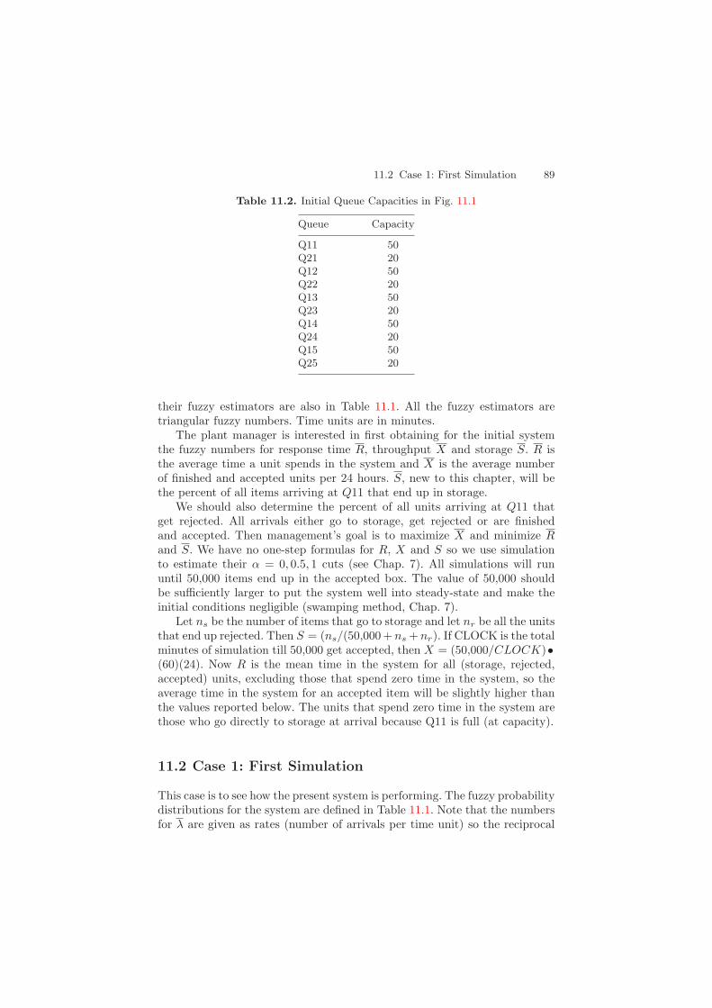
11.2 Case 1: First Simulation 89
Table 11.2. Initial Queue Capacities in Fig. 11.1
Queue Capacity
Q11 50Q21 20Q12 50Q22 20Q13 50Q23 20Q14 50Q24 20Q15 50Q25 20
their fuzzy estimators are also in Table 11.1. All the fuzzy estimators aretriangular fuzzy numbers. Time units are in minutes.
The plant manager is interested in first obtaining for the initial systemthe fuzzy numbers for response time R, throughput X and storage S. R isthe average time a unit spends in the system and X is the average numberof finished and accepted units per 24 hours. S, new to this chapter, will bethe percent of all items arriving at Q11 that end up in storage.
We should also determine the percent of all units arriving at Q11 thatget rejected. All arrivals either go to storage, get rejected or are finishedand accepted. Then management’s goal is to maximize X and minimize Rand S. We have no one-step formulas for R, X and S so we use simulationto estimate their α = 0, 0.5, 1 cuts (see Chap. 7). All simulations will rununtil 50,000 items end up in the accepted box. The value of 50,000 shouldbe sufficiently larger to put the system well into steady-state and make theinitial conditions negligible (swamping method, Chap. 7).
Let ns be the number of items that go to storage and let nr be all the unitsthat end up rejected. Then S = (ns/(50,000 + ns + nr). If CLOCK is the totalminutes of simulation till 50,000 get accepted, then X = (50,000/CLOCK)•(60)(24). Now R is the mean time in the system for all (storage, rejected,accepted) units, excluding those that spend zero time in the system, so theaverage time in the system for an accepted item will be slightly higher thanthe values reported below. The units that spend zero time in the system arethose who go directly to storage at arrival because Q11 is full (at capacity).
11.2 Case 1: First Simulation
This case is to see how the present system is performing. The fuzzy probabilitydistributions for the system are defined in Table 11.1. Note that the numbersfor λ are given as rates (number of arrivals per time unit) so the reciprocal

90 11 Machine Shop I
is the average time between arrivals. The values for µ are the mean servicetimes. Recall (Chap. 8) that we will use crisp estimators for the standarddeviation of the normal distribution. Using Chap. 8 we know how to chooseλ, µ11, µ21, . . . , µ25 to approximate the end points of the α-cuts of R andX. We need to determine this for S also, and how to pick the values forthe pi and qi, 1 ≤ i ≤ 5. Let S[α] = [s1(α), s2(α)]. We found that min(λ),min(µ)ij gives s1(α) and max(λ), max(µ)ij is for s2(α). We will have toexperiment with the pi and qi values, because they will depend on λ andthe µij , to approximate the end points of the alpha-cuts. We ran simulationsusing max/min values of λ, µij , pi and the qi to see what combinationsproduce the max/min of R, X and S. These results are in Tables 11.3 and11.4. In the tables: (1) “min” means use the left end point of the intervalfor the α-cut of the fuzzy estimator; and (2) “max” means use the right endpoint. In Table 11.3 “max/min” means both values give the same result. Theinformation in Tables 11.3 and 11.4 can now be used to estimate alpha-cutsof R, X and S with the simulation results in Table 11.5. If there are alternateoptimal solutions for the values of the parameters we only list one solution.
The value of CLOCK and the run time varies with the values of theparameters. However, the simulation is usually between 90 and 100 days(24 hours per day of production) and the run time varied from 2 seconds to13 seconds.
Table 11.3. Values of the Parameters for Min R, X, S
Min λ µij pi qi
R min min max maxX min max max maxS min min max/min max/min
Table 11.4. Values of the Parameters for Max R, X, S
Max λ µij pi qi
R max max min minX max min min minS max max min min
Table 11.5. Case 1 Simulation Alpha-Cuts of R, X, S
Item α = 0 Cut α = 0.5 Cut α = 1 Cut
R [15, 334] [32, 314] 250
X [501, 727] [542, 647] 591
S [0.00, 39.1] [0.00, 27.7] 12.9
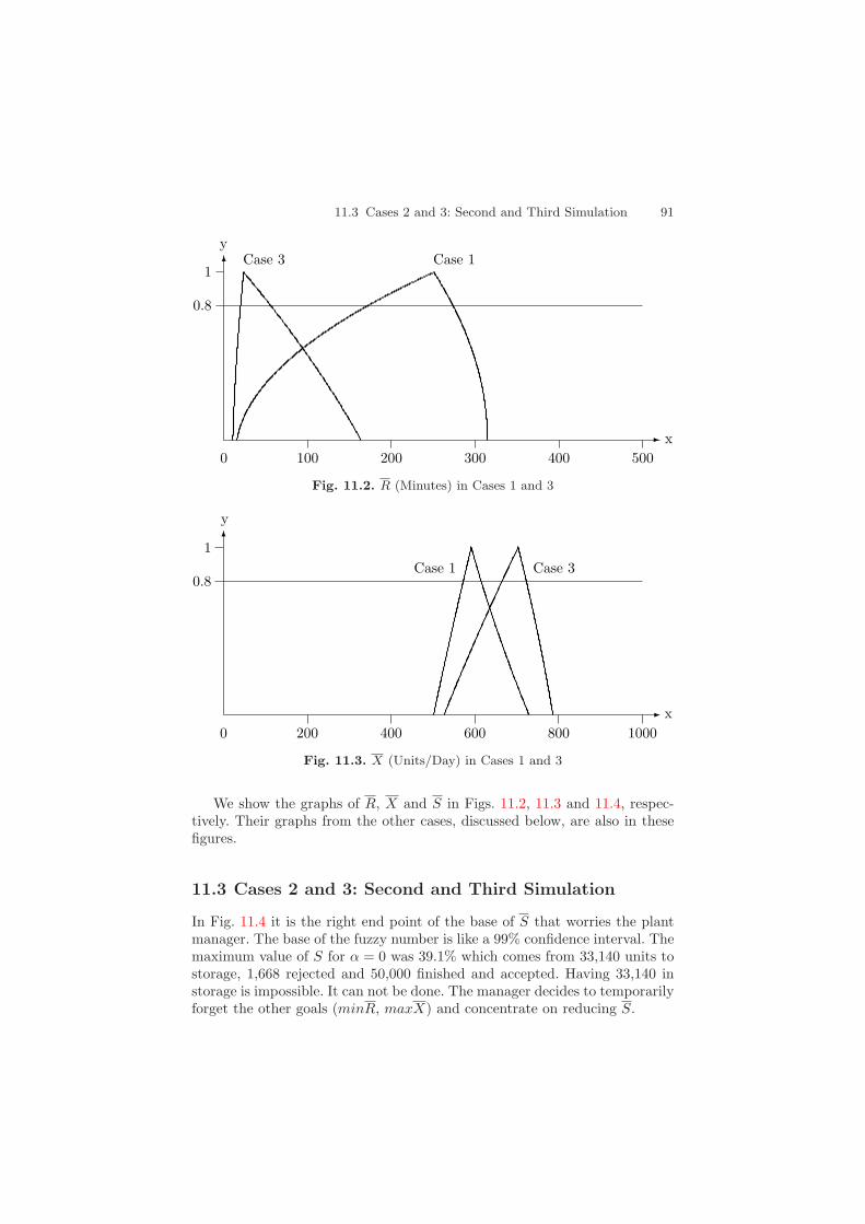
11.3 Cases 2 and 3: Second and Third Simulation 91
0 100 200 300 400 500x
1
0.8
yCase 1Case 3
Fig. 11.2. R (Minutes) in Cases 1 and 3
0 200 400 600 800 1000x
1
0.8
y
Case 3Case 1
Fig. 11.3. X (Units/Day) in Cases 1 and 3
We show the graphs of R, X and S in Figs. 11.2, 11.3 and 11.4, respec-tively. Their graphs from the other cases, discussed below, are also in thesefigures.
11.3 Cases 2 and 3: Second and Third Simulation
In Fig. 11.4 it is the right end point of the base of S that worries the plantmanager. The base of the fuzzy number is like a 99% confidence interval. Themaximum value of S for α = 0 was 39.1% which comes from 33,140 units tostorage, 1,668 rejected and 50,000 finished and accepted. Having 33,140 instorage is impossible. It can not be done. The manager decides to temporarilyforget the other goals (minR, maxX) and concentrate on reducing S.
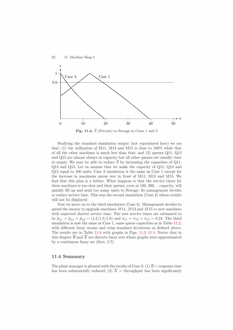
92 11 Machine Shop I
0 10 20 30 40 50x
1
0.8
y
Case 3 Case 1
Fig. 11.4. S (Percent) to Storage in Cases 1 and 3
Studying the standard simulation output (not reproduced here) we seethat: (1) the utilization of M11, M13 and M15 is close to 100% while thatof all the other machines is much less than that; and (2) queues Q11, Q13and Q15 are almost always at capacity but all other queues are usually closeto empty. We may be able to reduce S by increasing the capacities of Q11,Q13 and Q15. Let us assume that we make the capacity of Q11, Q13 andQ15 equal to 100 units. Case 2 simulation is the same as Case 1 except forthe increase in maximum queue size in front of M11, M13 and M15. Wefind that this plan is a failure. What happens is that the service times forthese machines is too slow and their queues, even at 100, 200, . . capacity, willquickly fill up and send too many units to Storage. So management decidesto reduce service time. This was the second simulation (Case 2) whose resultswill not be displayed.
Now we move on to the third simulation (Case 3). Management decides tospend the money to upgrade machines M11, M13 and M15 to new machineswith expected shorter service time. The new service times are estimated tobe µ11 = µ13 = µ15 = (1.2/1.5/1.8) and σ11 = σ13 = σ15 = 0.24. The thirdsimulation is now the same as Case 1, same queue capacities as in Table 11.2,with different fuzzy means and crisp standard deviations as defined above.The results are in Table 11.6 with graphs in Figs. 11.2–11.4. Notice that inthis chapter R and X are discrete fuzzy sets whose graphs were approximatedby a continuous fuzzy set (Sect. 2.7).
11.4 Summary
The plant manager is pleased with the results of Case 3: (1) R = response timehas been substantially reduced; (2) X = throughput has been significantly

Reference 93
Table 11.6. Case 3 Simulation Alpha-Cuts of R, X, S
Item α = 0 Cut α = 0.5 Cut α = 1 Cut
R [10, 163] [13, 107] 23
X [525, 785] [605, 752] 702
S [0, 19.5] [0, 6.0] 0
increased; and (3) S = percent into storage has also been greatly decreased.However, maxS[0] = 19.5% is still high. So, before management spends allthat money to obtain new machines they want to explore other alternatives.One alternative suggested by the engineers is to put the production line intoanother configuration (rearrange the machines). This will be the topic of thenext chapter.
Reference
1. H.A. Taha: Operations Research, Fifth Edition, Macmillan, N.Y., 1992. 87

12 Machine Shop II
12.1 Introduction
This chapter continues the machine shop model discussed in the previouschapter. Management is considering a radical change in the machine shopdiscussed in Chap. 11. The new setup is shown in Fig. 12.1. All the machinesM21, M22, M23, M24, M25 will be put into one group of three machinesM31, M32 and M33. Service station M3 will consist of the three parallel andidentical servers M31, M32, M33. The workers in M3 will be trained to serviceunits from all the five machines M11, . . . ,M15. This will produce a savings oftwo machines and this savings will be put into new machines M11a for M11,M13a for M13 and M15a for M15 all having faster service times.
Arrive Q11
M11 Q121 − p1
p1
Storage
Q3
M3
q
Reject
1 − p5Accept
1 − q
1 − q
Fig. 12.1. Machine Shop II Model
The new service times for M31, M32, M33 and M11a, M13a, M15a areall estimated by “experts”. Since we do not have any data on these newmachines we ask certain experts to estimate their service time. That is,we have no statistical data to generate the fuzzy numbers from a set of
James J. Buckley: Simulating Fuzzy Systems, StudFuzz 171, 95–101 (2005)www.springerlink.com c© Springer-Verlag Berlin Heidelberg 2005
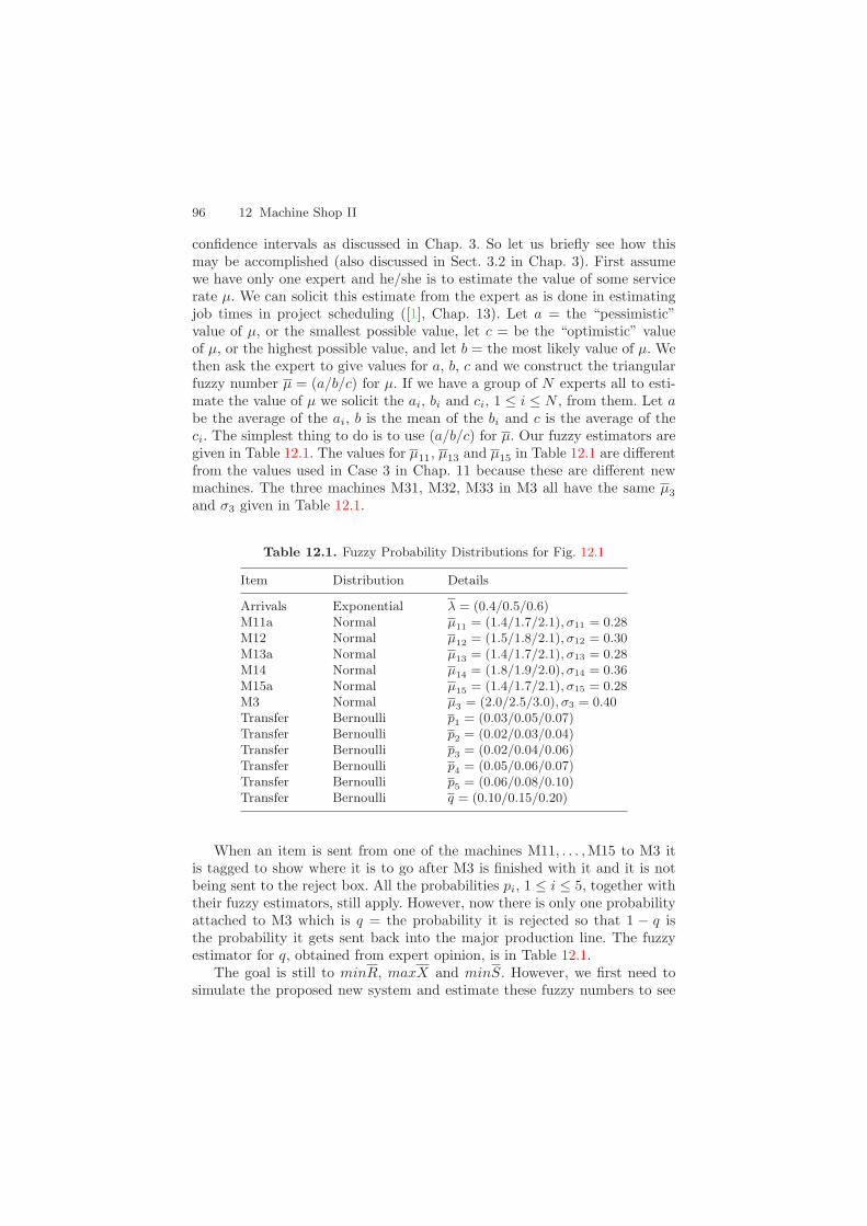
96 12 Machine Shop II
confidence intervals as discussed in Chap. 3. So let us briefly see how thismay be accomplished (also discussed in Sect. 3.2 in Chap. 3). First assumewe have only one expert and he/she is to estimate the value of some servicerate µ. We can solicit this estimate from the expert as is done in estimatingjob times in project scheduling ([1], Chap. 13). Let a = the “pessimistic”value of µ, or the smallest possible value, let c = be the “optimistic” valueof µ, or the highest possible value, and let b = the most likely value of µ. Wethen ask the expert to give values for a, b, c and we construct the triangularfuzzy number µ = (a/b/c) for µ. If we have a group of N experts all to esti-mate the value of µ we solicit the ai, bi and ci, 1 ≤ i ≤ N , from them. Let abe the average of the ai, b is the mean of the bi and c is the average of theci. The simplest thing to do is to use (a/b/c) for µ. Our fuzzy estimators aregiven in Table 12.1. The values for µ11, µ13 and µ15 in Table 12.1 are differentfrom the values used in Case 3 in Chap. 11 because these are different newmachines. The three machines M31, M32, M33 in M3 all have the same µ3
and σ3 given in Table 12.1.
Table 12.1. Fuzzy Probability Distributions for Fig. 12.1
Item Distribution Details
Arrivals Exponential λ = (0.4/0.5/0.6)M11a Normal µ11 = (1.4/1.7/2.1), σ11 = 0.28M12 Normal µ12 = (1.5/1.8/2.1), σ12 = 0.30M13a Normal µ13 = (1.4/1.7/2.1), σ13 = 0.28M14 Normal µ14 = (1.8/1.9/2.0), σ14 = 0.36M15a Normal µ15 = (1.4/1.7/2.1), σ15 = 0.28M3 Normal µ3 = (2.0/2.5/3.0), σ3 = 0.40Transfer Bernoulli p1 = (0.03/0.05/0.07)Transfer Bernoulli p2 = (0.02/0.03/0.04)Transfer Bernoulli p3 = (0.02/0.04/0.06)Transfer Bernoulli p4 = (0.05/0.06/0.07)Transfer Bernoulli p5 = (0.06/0.08/0.10)Transfer Bernoulli q = (0.10/0.15/0.20)
When an item is sent from one of the machines M11, . . . ,M15 to M3 itis tagged to show where it is to go after M3 is finished with it and it is notbeing sent to the reject box. All the probabilities pi, 1 ≤ i ≤ 5, together withtheir fuzzy estimators, still apply. However, now there is only one probabilityattached to M3 which is q = the probability it is rejected so that 1 − q isthe probability it gets sent back into the major production line. The fuzzyestimator for q, obtained from expert opinion, is in Table 12.1.
The goal is still to minR, maxX and minS. However, we first need tosimulate the proposed new system and estimate these fuzzy numbers to see
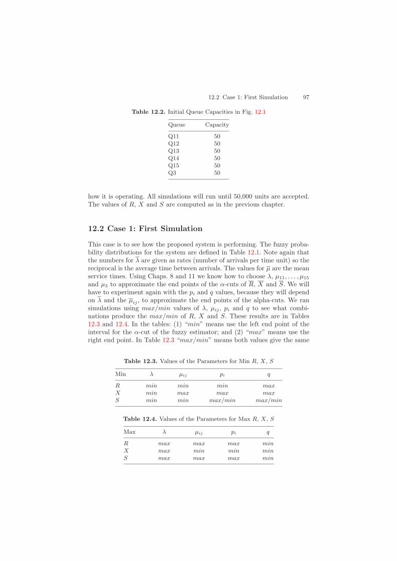
12.2 Case 1: First Simulation 97
Table 12.2. Initial Queue Capacities in Fig. 12.1
Queue Capacity
Q11 50Q12 50Q13 50Q14 50Q15 50Q3 50
how it is operating. All simulations will run until 50,000 units are accepted.The values of R, X and S are computed as in the previous chapter.
12.2 Case 1: First Simulation
This case is to see how the proposed system is performing. The fuzzy proba-bility distributions for the system are defined in Table 12.1. Note again thatthe numbers for λ are given as rates (number of arrivals per time unit) so thereciprocal is the average time between arrivals. The values for µ are the meanservice times. Using Chaps. 8 and 11 we know how to choose λ, µ11, . . . , µ15
and µ3 to approximate the end points of the α-cuts of R, X and S. We willhave to experiment again with the pi and q values, because they will dependon λ and the µij , to approximate the end points of the alpha-cuts. We ransimulations using max/min values of λ, µij , pi and q to see what combi-nations produce the max/min of R, X and S. These results are in Tables12.3 and 12.4. In the tables: (1) “min” means use the left end point of theinterval for the α-cut of the fuzzy estimator; and (2) “max” means use theright end point. In Table 12.3 “max/min” means both values give the same
Table 12.3. Values of the Parameters for Min R, X, S
Min λ µij pi q
R min min min maxX min max max maxS min min max/min max/min
Table 12.4. Values of the Parameters for Max R, X, S
Max λ µij pi q
R max max max minX max min min minS max max max min

98 12 Machine Shop II
Table 12.5. Case 1 Simulation Alpha-Cuts of R, X, S
Item α = 0 Cut α = 0.5 Cut α = 1 Cut
R [12.5, 310.9] [25.2, 189.9] 175
X [528, 714] [600, 683] 654
S [0.00, 34.74] [0.00, 19.32] 4.8
result. The information in Tables 12.3 and 12.4 can now be used to estimatealpha-cuts of R, X and S with the simulation results in Table 12.5.
In a simulation the value of CLOCK and the run time varies with thevalues of the parameters. Time units are in minutes. However, the simulationis usually between 90 and 100 days (24 hours per day of production) and therun time varied from 2 seconds to 13 seconds.
We show the graphs of R, X and S in Figs. 12.2, 12.3 and 12.4, respec-tively. Their graphs from the other cases, discussed below, are also in thesefigures. A sample GPSS program used in this chapter is in Chap. 28.
0.8
0 60 120 180 240 300x
1
y
Case 3
Case 1Case 2
Fig. 12.2. R (Minutes) in Cases 1, 2, 3
12.3 Case 2: Second Simulation
Management is really worried about the results on storage. The base of S islike a 99% confidence interval and the right end point of about 35% corre-sponding to 27,709 units sent to storage. This is not possible since there isno room to hold that many items. As the number of items in storage growsproduction would need to be halted to process these storage units and theplant manager does not wish to stop the production line.

12.3 Case 2: Second Simulation 99
0.8
0 200 400 600 800 1000x
1
y
Case 3
Case 1 Case 2
Fig. 12.3. X (Units/Day) in Cases 1, 2, 3
0.8
0 10 20 30 40 50x
1
y
Case 3
Case 1
Case 2
Fig. 12.4. S (Percent) to Storage in Cases 1, 2, 3
We notice from the standard simulation output that the machines in M3are not being fully utilized. So let us consider deleting two machines fromM3. The savings from this change will be put into decreasing the servicetimes on machines M11a, . . . ,M15a. The engineers think they can improvethe service times slightly to: µ11 = (1.3/1.4/1.5), µ12 = (1.4/1.5/1.6), µ13 =(1.3/1.4/1.5), µ14 = (1.4/1.5/1.6), µ15 = (1.3/1.4/1.5). The correspondingstandard deviations are σ11 = 0.26, σ12 = 0.28, σ13 = 0.26, σ14 = 0.28,σ15 = 0.26. These will be the only changes from Case 1. Now simulate thesystem to estimate S and R, X. The results are in Table 12.6 and Figs. 12.2–12.4.

100 12 Machine Shop II
Table 12.6. Case 2 Simulation Alpha-Cuts of R, X, S
Item α = 0 Cut α = 0.5 Cut α = 1 Cut
R [9.5, 101.2] [11.5, 65.4] 16.4
X [534, 850] [608, 764] 686
S [0.00, 13.64] [0.00, 1.25] 0.00
12.4 Case 3: Third Simulation
Management is now satisfied with storage. The base of S, like a 99% con-fidence interval, is [0.00, 13.64] with the point estimate (where membershipvalue is one), zero percent. They do not expect storage to be much more that0%. Also, R has decreased considerably in Case 2 (Fig. 12.2). How can weincrease throughput X without increasing S and R? Notice that Case 2 didnot substantially increase X (Fig. 12.3). The engineers say that there is noway to further decrease the service times for machines M11a, . . . ,M15a. Ifwe increase the arrival rate we will probably increase congestion in the sys-tem and therefore increase S and R. We might increase the queue capacityQ11, . . . ,Q15, but this will surely increase R. The engineers come up with avery expensive suggestion: replace machines M11a, . . . ,M15a with completelyrobotic machines RM11, . . . ,RM15.
Service times for the new robotic machines RM11, . . . ,RM15 are unknownbut will follow the uniform probability distribution. Using expert opinion wecome up with a fuzzy uniform (Sect. 3.5.5) distribution for service time forRM11, . . . ,RM15 shown in Table 12.7. We will use the same service timeas in Case 2 for the machine in M3 and the same pi and q values givenin Case 1. With these faster robotic machines we may consider increasingthe arrival rate. We believe that we can change λ to (0.5/0.6/0.7) which isthe new rate of arrivals per minute. We need to reinterpret Tables 12.3 and12.4 for the fuzzy uniform distribution. Min under µij means use the leftend points of a1j [0] and b1j [0] and max under µij means use the right endpoints. Queue capacities are the same as in Table 12.2. Now we are readyto simulate the fuzzy system to estimate X and R, S. The results are in
Table 12.7. Fuzzy Uniform Probability Distributions for Case 3
Item Distribution a b
RM11 Uniform a11 = (0.9/1.0/1.1) b11 = (1.1/1.2/1.3)
RM12 Uniform a12 = (1.0/1.1/1.2) b12 = (1.2/1.3/1.4)
RM13 Uniform a13 = (0.9/1.0/1.1) b13 = (1.1/1.2/1.3)
RM14 Uniform a14 = (1.0/1.1/1.2) b14 = (1.2/1.3/1.4)
RM15 Uniform a15 = (0.9/1.0/1.1) b15 = (1.1/1.2/1.3)

Reference 101
Table 12.8. Case 3 Simulation Alpha-Cuts of R, X, S
Item α = 0 Cut α = 0.5 Cut α = 1 Cut
R [7.1, 77.8] [7.7, 24.8] 11.3
X [671, 980] [738, 906] 829
S [0.00, 8.08] [0.00, 0.02] 0.00
Table 12.8 and Figs. 12.2–12.4. In this chapter X is a discrete fuzzy setwhose graph is approximated by a continuous fuzzy set (Sect. 2.7).
12.5 Summary
Let Ri, Xi and Si be the results from Cases i = 1, 2, 3. From our methodof ranking fuzzy numbers in Sect. 2.5 we see from Figs. 12.2–12.4 that: (1)R2 ≈ R3 < R1; (2) X1 ≈ X2 < X3; and (3) S2 ≈ S3 < S1. The bases ofthese fuzzy numbers are like 99% confidence intervals. Clearly, managementprefers Case 3 to Cases 1 and 2.
Now we compare these results to those in Chap. 11. We compare: (1)Fig. 11.2 and Fig. 12.2 for R; (2) Fig. 11.3 and Fig. 12.3 for X; and (3)Fig. 11.4 and Fig. 12.4 for S. The result is that Case 3 of Chap. 12 is thebest. So, the plant manager now needs to go to corporate headquarters tosecure the funds needed to implement Case 3.
Reference
1. H.A. Taha: Operations Research, Fifth Edition, Macmillan, N.Y., 1992. 96

13 Emergency Room Model
13.1 Introduction
The system in this chapter was adapted from an example in [1]. The flowthrough the system is shown in Fig. 13.1. Patients arrive, according to theexponential distribution, by coming through the front door or by ambulance.We model this emergency room during its busiest eight hour shift. All patientsare classified as A or B. All ambulance patients are classified as A patients.When a patient comes through the front door a nurse (N in Fig. 13.1) im-mediately assigns them as a class A, or B, patient. We assume there is nosignificant time delay in this initial classification.
Class B patients first go to the “sign in” procedure (S in Fig. 13.1) wherea secretary gets their basic information. After the sign in class B patientsproceed to an evaluation station manned by nurses (E in Fig. 13.1). Weassume that all service stations have unlimited waiting room preceding them.This emergency room will not turn any patients away because of limitedqueue capacity. When it gets busy patients can sit on the floor, wait in thehalls or even wait outside. Because all queues have infinite capacity they werenot shown in Fig. 13.1. Also, all service times will be modelled by the normaldistribution.
All patients will go to T1 in Fig. 13.1. T1 is where the patient is trans-ported to a “room” for treatment. There are n treatment rooms and thistransfer is handled by an emergency room assistant. Right now there aren = 6 treatment rooms and hospital management is not considering addingmore rooms. Once inside the treatment area class B patients go through “pa-per work”, P1 in Fig. 13.1, which is done by nurses. All patients are thentreated by doctors and nurses (T2 in Fig. 13.1). After treatment class B pa-tients are released or admitted to the hospital, but class A patients now havethe “paper work” done (P2 in Fig. 13.1), which is handled by nurses, beforerelease/admit. The operation of release/admit is assumed to have no timedelay.
Hospital management wants to “optimize” their emergency room. Theyhave too many complaints about their emergency room takes too much time.Their goals are to minimize R = mean time spent in the emergency roomand minimize costs. Since we do not have any one-step formulas for R inthis model we will simulate it to estimate alpha-cuts of R (see Chap. 7). The
James J. Buckley: Simulating Fuzzy Systems, StudFuzz 171, 103–109 (2005)www.springerlink.com c© Springer-Verlag Berlin Heidelberg 2005

104 13 Emergency Room Model
Ambulance A
Front Door A
Front Door B
Arrivals
S
E
T1
N
N
A
P1
B
B
T2 A
P2 ARelease/Admit
B
Fig. 13.1. Emergency Room
costs associated with this system will be the personnel costs for one eighthour shift. This cost will be crisp and not fuzzy. Personnel costs are made upfrom the secretaries, nurses, emergency room assistants and doctors. Thesehourly costs, including fringe benefit expenses, etc. are in Table 12.1.
These two goals will be in conflict. To reduce R we add more personnelwhich increases the cost. Management decides that reducing R is twice asimportant than minimizing costs. So our objective now is to
min[Z = τ1R + τ2Costs] , (13.1)
for τi > 0 and τ1 + τ2 = 1, with special interest for τ1 = 2/3, τ1 = 1/3. Nowfind the personnel assignments to minimize Z for selected values of the τi.
All simulations will attempt to run until 50,000 patients are in the boxrelease/admit. We need to run the simulation a long time so as not to biasR with the start-up results of all servers empty (the swamping method inChap. 7).
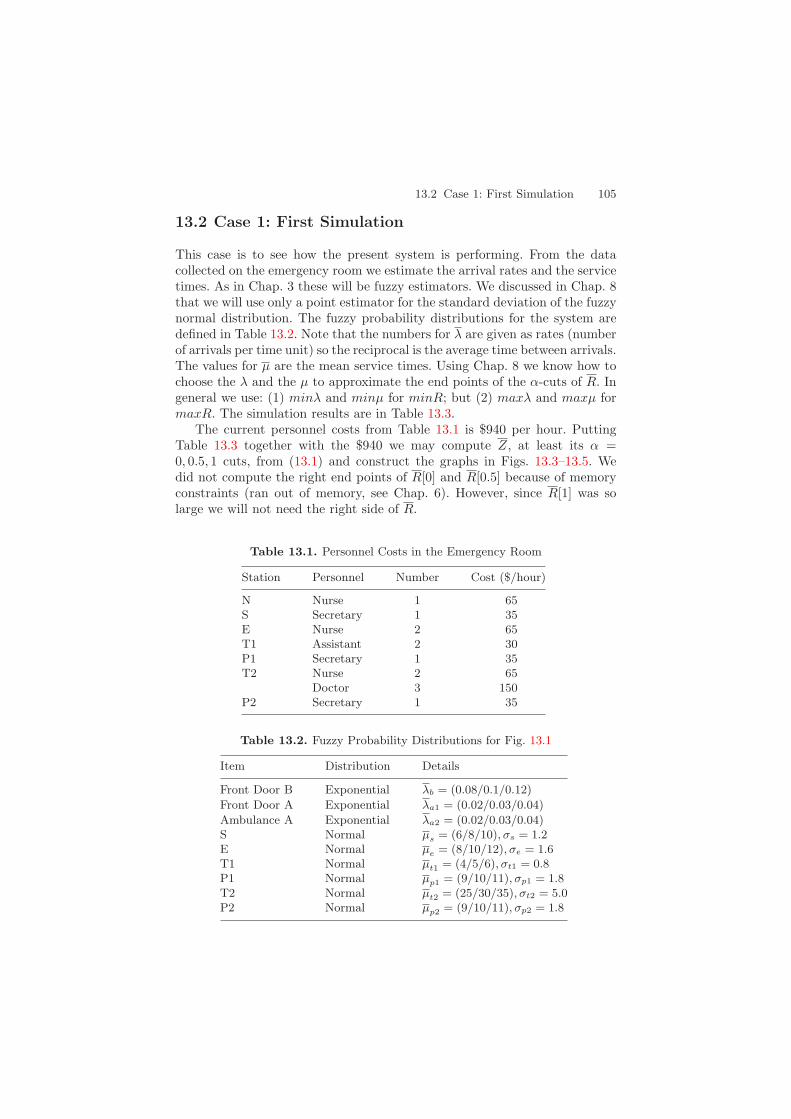
13.2 Case 1: First Simulation 105
13.2 Case 1: First Simulation
This case is to see how the present system is performing. From the datacollected on the emergency room we estimate the arrival rates and the servicetimes. As in Chap. 3 these will be fuzzy estimators. We discussed in Chap. 8that we will use only a point estimator for the standard deviation of the fuzzynormal distribution. The fuzzy probability distributions for the system aredefined in Table 13.2. Note that the numbers for λ are given as rates (numberof arrivals per time unit) so the reciprocal is the average time between arrivals.The values for µ are the mean service times. Using Chap. 8 we know how tochoose the λ and the µ to approximate the end points of the α-cuts of R. Ingeneral we use: (1) minλ and minµ for minR; but (2) maxλ and maxµ formaxR. The simulation results are in Table 13.3.
The current personnel costs from Table 13.1 is $940 per hour. PuttingTable 13.3 together with the $940 we may compute Z, at least its α =0, 0.5, 1 cuts, from (13.1) and construct the graphs in Figs. 13.3–13.5. Wedid not compute the right end points of R[0] and R[0.5] because of memoryconstraints (ran out of memory, see Chap. 6). However, since R[1] was solarge we will not need the right side of R.
Table 13.1. Personnel Costs in the Emergency Room
Station Personnel Number Cost ($/hour)
N Nurse 1 65S Secretary 1 35E Nurse 2 65T1 Assistant 2 30P1 Secretary 1 35T2 Nurse 2 65
Doctor 3 150P2 Secretary 1 35
Table 13.2. Fuzzy Probability Distributions for Fig. 13.1
Item Distribution Details
Front Door B Exponential λb = (0.08/0.1/0.12)
Front Door A Exponential λa1 = (0.02/0.03/0.04)
Ambulance A Exponential λa2 = (0.02/0.03/0.04)S Normal µs = (6/8/10), σs = 1.2E Normal µe = (8/10/12), σe = 1.6T1 Normal µt1 = (4/5/6), σt1 = 0.8P1 Normal µp1 = (9/10/11), σp1 = 1.8T2 Normal µt2 = (25/30/35), σt2 = 5.0P2 Normal µp2 = (9/10/11), σp2 = 1.8
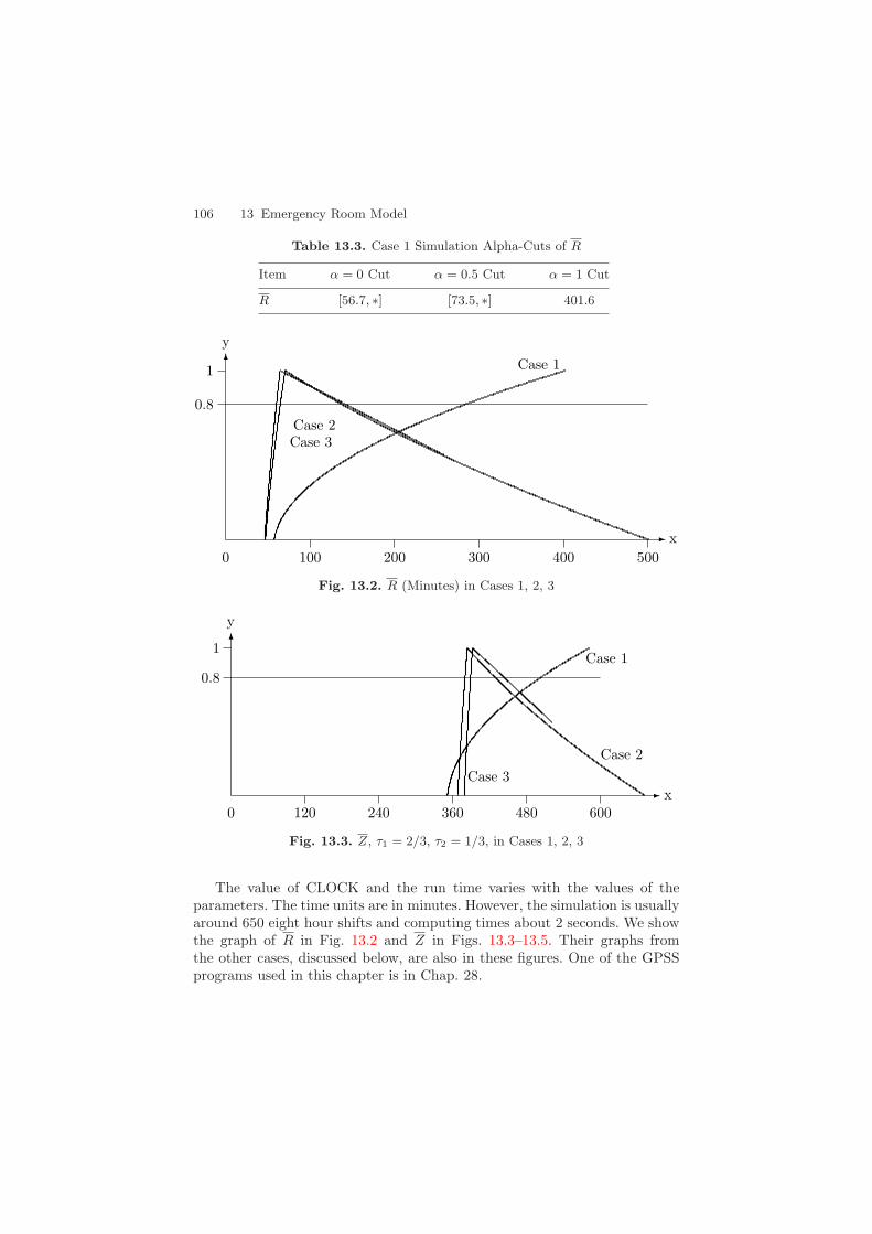
106 13 Emergency Room Model
Table 13.3. Case 1 Simulation Alpha-Cuts of R
Item α = 0 Cut α = 0.5 Cut α = 1 Cut
R [56.7, ∗] [73.5, ∗] 401.6
0.8
0 100 200 300 400 500x
1
y
Case 3
Case 1
Case 2
Fig. 13.2. R (Minutes) in Cases 1, 2, 3
0.8
0 120 240 360 480 600x
1
y
Case 3
Case 1
Case 2
Fig. 13.3. Z, τ1 = 2/3, τ2 = 1/3, in Cases 1, 2, 3
The value of CLOCK and the run time varies with the values of theparameters. The time units are in minutes. However, the simulation is usuallyaround 650 eight hour shifts and computing times about 2 seconds. We showthe graph of R in Fig. 13.2 and Z in Figs. 13.3–13.5. Their graphs fromthe other cases, discussed below, are also in these figures. One of the GPSSprograms used in this chapter is in Chap. 28.
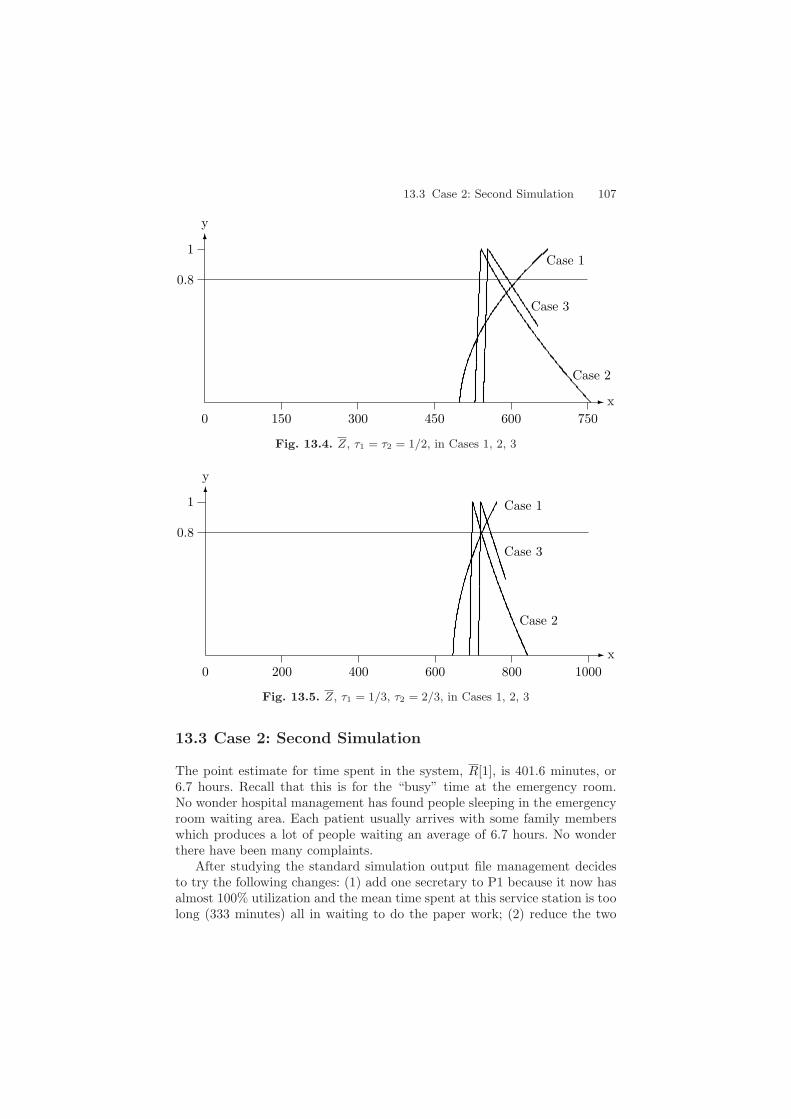
13.3 Case 2: Second Simulation 107
0.8
0 150 300 450 600 750x
1
y
Case 3
Case 1
Case 2
Fig. 13.4. Z, τ1 = τ2 = 1/2, in Cases 1, 2, 3
0.8
0 200 400 600 800 1000x
1
y
Case 3
Case 1
Case 2
Fig. 13.5. Z, τ1 = 1/3, τ2 = 2/3, in Cases 1, 2, 3
13.3 Case 2: Second Simulation
The point estimate for time spent in the system, R[1], is 401.6 minutes, or6.7 hours. Recall that this is for the “busy” time at the emergency room.No wonder hospital management has found people sleeping in the emergencyroom waiting area. Each patient usually arrives with some family memberswhich produces a lot of people waiting an average of 6.7 hours. No wonderthere have been many complaints.
After studying the standard simulation output file management decidesto try the following changes: (1) add one secretary to P1 because it now hasalmost 100% utilization and the mean time spent at this service station is toolong (333 minutes) all in waiting to do the paper work; (2) reduce the two

108 13 Emergency Room Model
assistants in T1 to only one assistant because its utilization is only 40%; and(3) add another nurse to treatment (T2). The increase in personnel costs isjust $70 per hour so the total is $1010 per hour. The service time in T2 haschanged due to adding one nurse. Expert opinion (Sects. 3.2, 12.1) estimatesthe new fuzzy mean to be µt2 = (20/25/30) with σt2 = 4.0. Making thesechanges we simulate the new system with results in Table 13.4 and Figs. 13.2–13.5. In Table 13.4 the right end point of R[0] is 499.2∗ which means that itwas only a simulation run of 1000 patients because larger values resulted in“out of common”, or out of memory.
Table 13.4. Case 2 Simulation Alpha-Cuts of R
Item α = 0 Cut α = 0.5 Cut α = 1 Cut
R [46.2, 499.2∗] [54.5, 226.4] 69.7
13.4 Case 3: Third Simulation
Case two resulted in a point estimate for R of 69.7 minutes, or 1.16 hours.This is clearly a great improvement over the 6.7 hours in Case 1. Studyingthe standard simulation output we see only one further improvement withouta very great increase in costs. In S increase the number of secretaries fromone to two because too much time was spent waiting to sign in and right nowthis one secretary has almost 100% utilization. The costs go up by 35 perhour to a total of $1045 per hour. After this change we simulate the systemagain with the outcome in Table 13.5 and Figs. 13.2–13.5. In Table 13.5 theright end point of R[0] has a ∗ value meaning that we ran out of “common”(memory) even for a run of 1000 patients.
Table 13.5. Case 3 Simulation Alpha-Cuts of R
Item α = 0 Cut α = 0.5 Cut α = 1 Cut
R [45.3, ∗] [52.5, 257.5] 63.6
13.5 Summary
Let us look more closely at Case 3. Patient type B goes through S, E, T1, P1and T2 in Fig. 13.1. Add up the mean service times for these stations and weget 58 minutes. But R[1] = 63.6 minutes only 5.6 minutes more than the 58.Patient type A goes through T1, T2 and P2 in Fig. 13.1 with mean service

Reference 109
times adding up to 40 minutes 23.6 under the 63.6. Hospital managementlikes these results. However, there is still a possibility of long waits since theright end point of R[0] is large (probably more than 5 hours).
Next we study Figs. 13.2–13.5. Let Ri (Zi) be the value of R (Z) in Casei = 1, 2, 3. The bases of all these fuzzy numbers are like 99% confidenceintervals. The reader may need to review Sect. 2.5 of Chap. 2 on how we willorder (rank) fuzzy numbers. First, from Fig. 13.2, we see that R2 ≈ R3 < R1,which is no surprise. The next three figures show how we may treat thesituation of having two goals of minR and min(Costs). Figure 13.3 showswhere we weight R twice as much as “costs” and Z2 ≈ Z3 < Z1. In fact, Z2
and Z3 are almost identical. Next we weight R and “costs” equally and Z3 hasmoved a little to the right of Z2 but still Z2 ≈ Z3 < Z1. The last case is werewe weight “costs” twice as much as R and Fig. 13.5 shows Z1 ≈ Z2 ≈ Z3.Hospital management sees no clear choice in Cases 1, 2, 3 so they requestfurther possible changes in the system and more simulations.
Reference
1. Getting Started SIMPROCESS, CACI Products Company, San Diego, CA, 2004. 103

14 Machine Servicing Problem
14.1 Introduction
The machine servicing problem is shown in Fig. 14.1 and a basic descriptioncan be found in almost any operations research book ([1], p. 573). However,the model in this chapter is considerably different from that in [1]. Itemsarrive for processing at the first machine M1 and then proceed through thenext four machines M2. , , , M5 until they reach the “finished” box. All queuesin front of each machine are assumed to have unlimited capacity. Queuecapacity will not be of importance in this problem so we did not show anyqueue in Fig. 14.1. Each machine can break down and this will certainlyeffect throughput, but all other unbroken machines continue to function. Theprobability that machine Mi breaks down is pi, 1 ≤ i ≤ 5. For each machineMi the probability of a break down is modelled as follows: whenever an itemarrives at the machine for processing, and goes into queue if the machine isbusy, the machine can break down with probability pi, 1 ≤ i ≤ 5. If an itemis being processed at break down it waits until the machine is fixed and thenit continues its processing (no processing time is lost). There is a crew of kmachine repair workers in the “repair” station in Fig. 14.1. The goal is tofind the optimal k to minimize total costs.
Arrive
M1 1 − p1
M5
Finished1 − p5
Repair
p1
p5
Fig. 14.1. Machine Servicing Problem
In Fig. 14.1 it looks like a broken machine is sent to the repair stationfor repair. This is not true. When a machine breaks down and there is anavailable repair worker, the repair worker is sent to the machine for repair.
James J. Buckley: Simulating Fuzzy Systems, StudFuzz 171, 111–116 (2005)www.springerlink.com c© Springer-Verlag Berlin Heidelberg 2005

112 14 Machine Servicing Problem
The repair station is modelled as having k identical and parallel servers eachserver is a repair worker.
We may wish to add the possibility of defective items and limited queuecapacity later but in this chapter we concentrate on finding k to minimizetotal costs.
First there is the hourly cost of a repair person, plus their needed tools andsupplies, which we assume to be (including fringe benefits, etc.) 100 $/hour.Next is the cost of lost production due to broken machines and down time.All simulations will be run until there are 50,000 units in the finished box.We are using the “swamping” method discussed in Chap. 7. Time units arein minutes. CLOCK gives the total number of minutes in the simulation. LetW = (CLOCK)/(60)(8) = the number of 8 hour shifts in the simulation.If D = is the total number of broken machines per simulation, if T = themean repair time (both being repaired and waiting to be repaired) per brokenmachine, and if E = the cost ($/hour) of machine down time, then total cost(TC) per 8 hour shift is
TC(k) = k(100)(8) + [D/W ]TE . (14.1)
In this equation D, W and T will all depend on k. We know that some ofthese numbers will be fuzzy. In the simulations for fixed k we will vary certainparameters through their α-cuts producing variability in D, W , and T . Sothese will all be fuzzy sets/numbers. Also, E is a very difficult number toestimate and we employ expert opinion (see Sects. 3.2, 12.1) to get the fuzzyestimator E for E. Therefore, out goal is to minimize
TC(k) = 800k + [D/W ] T E , (14.2)
for k = 1, . . . , 5.Now we simulate the fuzzy system to estimate some alpha-cuts of TC(k).
There are one-step formulas (see Chap. 7) that can be derived for the machineservicing model in [1], but we do not have such functions for our model sinceit is quite different from [1]. Hence, crisp simulation is used to approximatethe fuzzy sets/numbers.
14.2 Case 1: First Simulation (k = 1)
The time it takes to fix a broken machine needs to be estimated from data.Therefore (Chap. 3) we obtain a fuzzy estimator for the mean repair time.We will use the fuzzy exponential to model arrivals, the fuzzy uniform formachine (M1, . . . ,M5) processing times and the fuzzy normal for repair times.The fuzzy parameters values are all given in Table 14.1. However, we assumethat the probability of a break down is known (crisp). We will use E =(125/150/175).
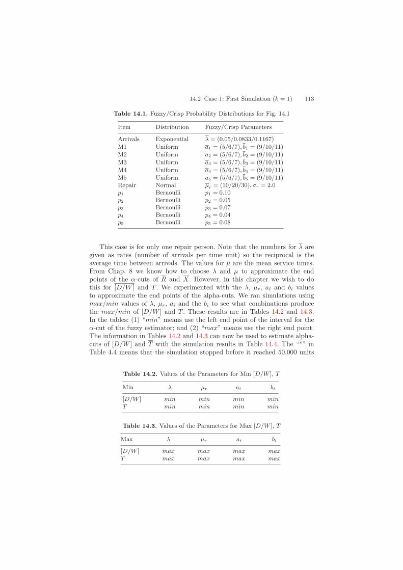
14.2 Case 1: First Simulation (k = 1) 113
Table 14.1. Fuzzy/Crisp Probability Distributions for Fig. 14.1
Item Distribution Fuzzy/Crisp Parameters
Arrivals Exponential λ = (0.05/0.0833/0.1167)
M1 Uniform a1 = (5/6/7), b1 = (9/10/11)
M2 Uniform a2 = (5/6/7), b2 = (9/10/11)
M3 Uniform a3 = (5/6/7), b3 = (9/10/11)
M4 Uniform a4 = (5/6/7), b4 = (9/10/11)
M5 Uniform a5 = (5/6/7), b5 = (9/10/11)Repair Normal µr = (10/20/30), σr = 2.0p1 Bernoulli p1 = 0.10p2 Bernoulli p2 = 0.05p3 Bernoulli p3 = 0.07p4 Bernoulli p4 = 0.04p5 Bernoulli p5 = 0.08
This case is for only one repair person. Note that the numbers for λ aregiven as rates (number of arrivals per time unit) so the reciprocal is theaverage time between arrivals. The values for µ are the mean service times.From Chap. 8 we know how to choose λ and µ to approximate the endpoints of the α-cuts of R and X. However, in this chapter we wish to dothis for [D/W ] and T . We experimented with the λ, µr, ai and bi valuesto approximate the end points of the alpha-cuts. We ran simulations usingmax/min values of λ, µr, ai and the bi to see what combinations producethe max/min of [D/W ] and T . These results are in Tables 14.2 and 14.3.In the tables: (1) “min” means use the left end point of the interval for theα-cut of the fuzzy estimator; and (2) “max” means use the right end point.The information in Tables 14.2 and 14.3 can now be used to estimate alpha-cuts of [D/W ] and T with the simulation results in Table 14.4. The “*” inTable 4.4 means that the simulation stopped before it reached 50,000 units
Table 14.2. Values of the Parameters for Min [D/W ], T
Min λ µr ai bi
[D/W ] min min min minT min min min min
Table 14.3. Values of the Parameters for Max [D/W ], T
Max λ µr ai bi
[D/W ] max max max maxT max max max max

114 14 Machine Servicing Problem
Table 14.4. Case 1 Simulation Alpha-Cuts of [D/W ], T , TC (1)
Item α = 0 Cut α = 0.5 Cut α = 1 Cut
[D/W ] [10.2, ∗] [10.9, 12.6] 11.7
T [11.2, ∗] [18.0, 40.4] 27.0
TC(1) [15,023.90, ∗] [27,846.52, 83,937.7] 48,088.01
Table 14.5. Case 2 Simulation Alpha-Cuts of [D/W ], T , TC (2)
Item α = 0 Cut α = 0.5 Cut α = 1 Cut
[D/W ] [10.2, 13.4] [10.8, 12.5] 11.9
T [10.0, 32.2] [15.1, 26.0] 20.5
TC(2) [12,827.38, 76,949.55] [24,068.04, 52,797.83] 38,149.66
Table 14.6. Case 3 Simulation Alpha-Cuts of [D/W ], T , TC (3)
Item α = 0 Cut α = 0.5 Cut α = 1 Cut
[D/W ] [10.1, 13.6] [10.9, 12.6] 11.7
T [10.0, 30.2] [15.0, 25.0] 20.0
TC(3) [15,000.00, 74,405.54] [24,978.79, 53,903.68] 37,604.08
Table 14.7. Case 4 Simulation Alpha-Cuts of [D/W ], T , TC (4)
Item α = 0 Cut α = 0.5 Cut α = 1 Cut
[D/W ] [10.1, 13.6] [10.8, 12.6] 11.7
T [10.0, 30.0] [15.0, 25.0] 20.0
TC(4) [15,793.70, 74,544.91] [25,470.36, 54,527.85] 38,300.14
in the finished box because it ran out of memory (Chap. 6). We calculatedthe α-cuts of TC(k) using more decimal places in the alpha-cuts of [D/W ]and T than the rounded off values in Tables 14.4–14.8.
The value of CLOCK and the run time varies with the values of theparameters. However, the simulation was usually around 1400 eight hourshifts and the run time varied from 1 to 2 seconds.
We show the graphs of TC(k), k = 1, . . . , 5, in Fig. 14.2.
14.3 Case 2: Second Simulation (k = 2)
We change k = 1 to k = 2 and simulate the fuzzy system again with resultsin Table 14.5.

14.7 Summary 115
Table 14.8. Case 5 Simulation Alpha-Cuts of [D/W ], T , TC (5)
Item α = 0 Cut α = 0.5 Cut α = 1 Cut
[D/W ] [10.1, 13.6] [10.8, 12.6] 11.6
T [10.0, 30.0] [15.0, 25.0] 20.0
TC(5) [16,639.71, 75,376.04] [26,270.36, 55,086.05] 38,768.68
0.8
1 2 3 4 5 6x
1
y
Case 3
Case 2Case 4
Case 1
Case 5
Fig. 14.2. TC(k) (Dollars) in Cases 1–5. Scale = x(10,000)
14.4 Case 3: Third Simulation (k = 3)
Now there are three repair workers. Simulation produces the α-cuts inTable 14.6.
14.5 Case 4: Fourth Simulation (k = 4)
The fourth simulation is for four repair workers and the alpha-cuts are shownin Table 14.7.
14.6 Case 5: Fifth Simulation (k = 5)
The last simulation is when there is five repair persons with α-cuts in Table14.8.
14.7 Summary
We see that [D/W ] is fairly constant for k = 1, . . . , 5 because the pi, theprobability of machine Mi breaking down, was assumed known and it was

116 14 Machine Servicing Problem
not fuzzy. Also, T , down time for a broken machine, was fairly constantfor k = 2, 3, 4, 5. The result is that the term [D/W ] T E in TC(k) wasapproximately level (constant) for k = 2, 3, 4, 5 and shows its largest changein going from k = 1 to k = 2 since T decreased. Now add the term 800k toget all of TC(k) with their graphs in Fig. 14.2.
In Fig. 14.2 all the fuzzy numbers intersect above the horizontal line at 0.8,see Fig. 2.4. The base of these fuzzy numbers is like a 99% confidence interval.We conclude that all of these fuzzy numbers are approximately equal. Ourmethod of ranking fuzzy numbers in Sect. 2.5 does not eliminate any cases.From Fig. 14.2 we probably agree to drop Case 1. With all the other casesalmost the same we recommend Case 2 because it has the least number ofworkers.
The above study ends phase I of the problem. Consider the assumptionthat all the pi are known and crisp and possibly make them fuzzy. Modelmachine break downs differently using the fuzzy exponential and independentof items arriving for processing. Maybe also add capacity constraints to allthe queues in front of all the machines. We could look at the hourly cost ofa repair person and consider it to be fuzzy. Go on to phase II.
Reference
1. H.A. Taha: Operations Research, Fifth Edition, Macmillan, N.Y., 1992. 111, 112
15 Life Insurance: New Account Model
15.1 Introduction
This problem was derived from an example in [1]. The system is shown inFig. 15.1. This figure shows how this insurance company handles an applica-tion for an insurance policy. New account applications arrive at the rate of λper unit time. We use the exponential to model time between arrivals with1/λ the mean time between arrivals. A new account first goes to the creditcheck (CC in Fig. 15.1) station. All service times will be modelled by thenormal distribution. The clerk at CC can reject the application, with prob-ability p1, or not reject and send it on to “SPLIT”. The SPLIT operationcreates a “clone” (an identical copy of the application) and sends one copy toRR (risk rating) and the other to M (medical check). The SPLIT operationis assumed to take no time, or there is no delay at SPLIT. The medical checkstation is staffed by medical doctors who review the medical history of theapplicant and the risk rating station has clerks who evaluate the company’srisk in the policy. After M and RR the two copies come together at JOINand proceed as one file.
The two copies of the application can arrive at JOIN at different times.The first copy to arrive at JOIN must wait there until its clone arrives for bothto be joined into one file. We assume that there is no significant time delay inthe joining operation once both copies are present. Once joined the file goesto the review station (R in Fig. 15.1). A clerk at R may reject the applicationwith probability p2, or send it on to the pricing station (P in the figure). Afterpricing the application proceeds to the paper work station (PW) where allthe relevant information is assembled into an insurance policy and the newaccount ends up in the approved box. It is assumed that all queues haveunlimited capacity and have not been shown in Fig. 15.1.
Management wants the time it takes to process an application to be mini-mized. They would like to investigate the staffing of the various work stationsto reduce R = mean time in the system for an any (rejected/approved) ap-plication. However, as they add more clerks to CC, RR, R and P the totalcosts increase. They would like to keep the costs within some target budgetwhile minimizing R.
Since we do not have any one-step formulas (Chap. 7) for R in this modelwe will simulate it to estimate α-cuts of R. The costs associated with this
James J. Buckley: Simulating Fuzzy Systems, StudFuzz 171, 117–121 (2005)www.springerlink.com c© Springer-Verlag Berlin Heidelberg 2005

118 15 Life Insurance: New Account Model
Arrive
CC
Reject
p1
1 − p1
SPLIT
M
RR
JOIN
R
p2
1-p2
P
PW Approved
Fig. 15.1. New Account Model
system will be the personnel costs for one eight hour shift. This cost will becrisp and not fuzzy. Personnel costs are made up from the secretaries, clerksand doctors. These hourly costs, including fringe benefit expenses, etc. arein Table 15.1. The budget constraint is $B per eight hour shift. So we wishto minR subject to Costs ≤ B. All simulations will be run until 50,000 newapplications have been processed. Simulation time is in minutes. We need torun the simulation a long time so as not to bias R with the start-up results ofall service stations empty (the swamping method Chap. 7). A simulation runof 50,000 is equal to approximately 300 eight hour shifts for the new accountdepartment. Also, each simulation runs takes around 2 seconds.
15.2 Case 1: First Simulation
This case is to see how the system will perform with minimal staffing. Mini-mal staffing is to use only one clerk/secretary/doctor at their service station.From the data collected on the new accounts department we estimate the ar-rival rates and the service times. These will be fuzzy estimators. We discussed
Table 15.1. Staffing Costs in the New Account Department
Station Personnel Cost($/hour)
CC Clerk 65M Doctor 150RR Clerk 65R Clerk 65P Clerk 65PW Secretary 50
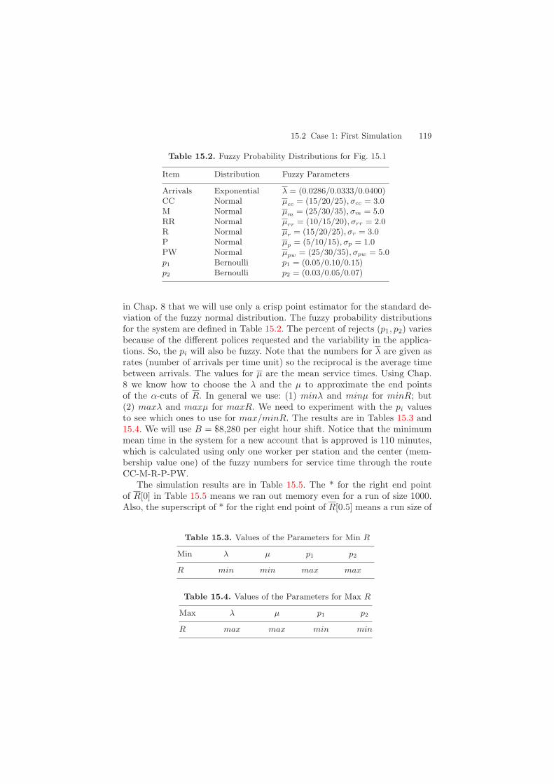
15.2 Case 1: First Simulation 119
Table 15.2. Fuzzy Probability Distributions for Fig. 15.1
Item Distribution Fuzzy Parameters
Arrivals Exponential λ = (0.0286/0.0333/0.0400)CC Normal µcc = (15/20/25), σcc = 3.0M Normal µm = (25/30/35), σm = 5.0RR Normal µrr = (10/15/20), σrr = 2.0R Normal µr = (15/20/25), σr = 3.0P Normal µp = (5/10/15), σp = 1.0PW Normal µpw = (25/30/35), σpw = 5.0p1 Bernoulli p1 = (0.05/0.10/0.15)p2 Bernoulli p2 = (0.03/0.05/0.07)
in Chap. 8 that we will use only a crisp point estimator for the standard de-viation of the fuzzy normal distribution. The fuzzy probability distributionsfor the system are defined in Table 15.2. The percent of rejects (p1, p2) variesbecause of the different polices requested and the variability in the applica-tions. So, the pi will also be fuzzy. Note that the numbers for λ are given asrates (number of arrivals per time unit) so the reciprocal is the average timebetween arrivals. The values for µ are the mean service times. Using Chap.8 we know how to choose the λ and the µ to approximate the end pointsof the α-cuts of R. In general we use: (1) minλ and minµ for minR; but(2) maxλ and maxµ for maxR. We need to experiment with the pi valuesto see which ones to use for max/minR. The results are in Tables 15.3 and15.4. We will use B = $8,280 per eight hour shift. Notice that the minimummean time in the system for a new account that is approved is 110 minutes,which is calculated using only one worker per station and the center (mem-bership value one) of the fuzzy numbers for service time through the routeCC-M-R-P-PW.
The simulation results are in Table 15.5. The * for the right end pointof R[0] in Table 15.5 means we ran out memory even for a run of size 1000.Also, the superscript of * for the right end point of R[0.5] means a run size of
Table 15.3. Values of the Parameters for Min R
Min λ µ p1 p2
R min min max max
Table 15.4. Values of the Parameters for Max R
Max λ µ p1 p2
R max max min min

120 15 Life Insurance: New Account Model
Table 15.5. Case 1 Simulation Alpha-Cuts of R
Item α = 0 Cut α = 0.5 Cut α = 1 Cut
R [94.6, ∗] [128.6, 1003.5∗] 263.8
1000 since larger values ran out of memory. With minimal staffing the costsper eight hour shift is $3, 680 well under budget.
We show the graphs of R in Fig. 15.2.
0.8
0 100 200 300 400 500x
1
y
Case 3
Case 1
Case 2
Fig. 15.2. R (Minutes) in Cases 1–3
15.3 Case 2: Second Simulation
In Case 1, from the standard simulation output file, we see that the utilizationof M is 0.903, of PW is 0.858 and of CC is 0.669. So, let us try two doctors inM, two clerks in CC and two secretaries in PW. The new total cost is $5800per eight hour shift, still under budget. Using this staffing, the simulationresults are in Table 15.6. Let Ri be the fuzzy value of R in Case i = 1, 2, 3.We get that R2 < R1, see Sect. 2.5, from Fig. 15.1.
We do not expect to make further substantial reductions in R since R[1] =113.9 and (as discussed above) the minimum α = 1 mean value of R is 110.However, the 110 figure was for one person at each service station and weadded more workers. Since we have some money left in the budget let us tryto reduce R further.

Reference 121
Table 15.6. Case 2 Simulation Alpha-Cuts of R
Item α = 0 Cut α = 0.5 Cut α = 1 Cut
R [77.0, 317.7] [93.3, 146.6] 113.9
15.4 Case 3: Third Simulation
We have found a way to spend all the money in the budget. It is: (1) threeclerks in CC; (2) two doctors in M; (3) two clerks in RR, R, P; and (4) threesecretaries in PW. The total cost is $8280 per eight hour shift and all themoney in the budget is gone. We are curious to see what happens with thisstaffing. Simulation results are in Table 15.7 and the graph of R3 (Case 3) isin Fig. 15.2.
Table 15.7. Case 3 Simulation Alpha-Cuts of R
Item α = 0 Cut α = 0.5 Cut α = 1 Cut
R [74.0, 143.3] [87.7, 120.2] 102.9
15.5 Summary
This chapter was about staffing work stations in a new account departmentin an insurance company. The objective was to minimize R, the fuzzy numberfor the time an application (rejected/approved) spends in the system, subjectto a fixed budget constraint. Three cases were studied with their resultsshown in Fig. 15.2. The base of these fuzzy numbers is like a 99% confidenceinterval. We see that R3 ≈ R2 < R1. Having only these three cases we firstrecommend Case 2 because it spends less money than Case 3. However, thereis some worry about the large value of the right end point of R2[0] whichimplies that we go with Case 3. Which case would you choose?
Reference
1. Getting Started SIMPROCESS, CACI Products Company, San Diego, CA, 2004. 117

16 Inventory Control I
16.1 Introduction
This single item multi-period inventory model is shown in Fig. 16.1. Thisproblem will be expanded and also studied in the next chapter. These in-ventory control models may be found in most operation research books([2], Chap. 14) and is chapter is modelled after the paper [1].
x1
z1
D1
x2 x3
z2
D2
z3
zN
DN
xN+1xN
Fig. 16.1. Inventory Control Problem I
We first describe the inventory problem in Fig. 16.1. The incoming inven-tory x1 will always be a given real number. The variables are the z1, . . . , zN
which are the amounts we are to order each period. The zi, 1 ≤ i ≤ N ,are non-negative integers. The Di represent the demand in the i-th periodand the xi, 2 ≤ i ≤ N , stands for the outgoing inventory, which will be thestarting inventory for the next period, in the i-th period. So we must have
xi+1 = xi + zi − Di, 1 ≤ i ≤ N , (16.1)
as long as xi+1 ≥ 0. If xi + zi − Di < 0, then we set xi+1 = 0.There are only N periods and at the end of the planning horizon man-
agement would like final inventory to be close to zero. That is, a goal is toobtain xN+1 = 0. We will model demand using the fuzzy normal distributionso let the fuzzy estimator of the mean be µ with crisp standard deviation σ.Since Di will be fuzzy, then the xi+1, i ≥ 1, in (16.1) will also be fuzzy, andhence xN+1 is also fuzzy. A goal is to minxN+1.
There are two basic assumptions in this chapter which will be relaxed inthe next chapter. First, we assume that there is zero delivery lag with instantreplenishment at the start of each period. During the i-th period we place
James J. Buckley: Simulating Fuzzy Systems, StudFuzz 171, 123–129 (2005)www.springerlink.com c© Springer-Verlag Berlin Heidelberg 2005

124 16 Inventory Control I
an order for zi units which all arrive at the start of the next period. Also,there is no backlogging. What this means is that if xi + zi −Di < 0, demandexceeds supply, these orders are lost and we do not carry these orders overto the next period’s demand. Another assumption, used in both chapters, isthat future money is treated as equal to present money and we will not usethe present value (discount future money back to the present).
The second goal is to minimize total inventory cost over the N periods.This cost is made up of four components: (1) purchase cost; (2) ordering cost;(3) holding cost; and (4) shortage cost. We now discuss these in detail.
We assume that we are to buy the item and we do not produce it ourselves.There may, or may not, be price breaks. For simplicity let us assume thatthere are no price breaks and it costs $10 per unit to purchase one unit.The ordering cost Ki in the i-th period is the cost of placing the order,checking up on the order and putting the items into inventory when theyarrive. This number is always difficult to estimate so we will model it usinga fuzzy number (obtained from expert opinion, Sects. 3.2, 12.1). Then thetotal cost of obtaining zi units at the start of the i-th period is
Ci(zi) =
0, zi = 0 ,
Ki + 10zi, zi > 0 ,(16.2)
for fuzzy Ki.The holding cost is assumed to be proportional to ending inventory. Let
hi be the holding cost per unit for the i-th period. This number, dependingon interest on invested capital, depreciation, etc., is very difficult to estimateexactly, so it will also be fuzzy. Through expert opinion let out fuzzy estimatorof the holding cost be hi. Hence the holding cost for the i-th period is
Hi(zi) = hi(xi + zi − Di) , (16.3)
as long as ending inventory is positive, otherwise the holding cost is zero.When we run out of inventory and demand exceeds supply, we have lost
sales and there is a penalty. Let pi be the penalty cost per lost sale whichincludes the money lost in the sale plus some amount for the loss of customer“good will”. This is another value almost impossible to estimate precisely, sowe will have a fuzzy estimator pi for the lost sales penalty. The lost sales costfor the i-th period is
Li(zi) = pi(Di − xi − zi) , (16.4)
as long as lost sales is positive, otherwise it is zero.The total inventory cost for the N periods is
TC =N∑
i=1
[Ci(zi) + Hi(zi) + Li(zi)] . (16.5)
The goal is to find the zi to minTC.
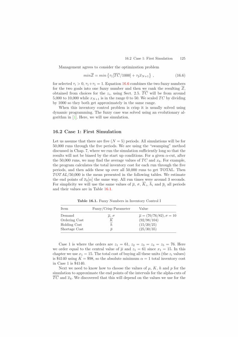
16.2 Case 1: First Simulation 125
Management agrees to consider the optimization problem
minZ = minτ1[TC/1000] + τ2xN+1
, (16.6)
for selected τi > 0, τ1+τ1 = 1. Equation 16.6 combines the two fuzzy numbersfor the two goals into one fuzzy number and then we rank the resulting Z,obtained from choices for the zi, using Sect. 2.5. TC will be from around5,000 to 10,000 while xN+1 is in the range 0 to 50. We scaled TC by dividingby 1000 so they both get approximately in the same range.
When this inventory control problem is crisp it is usually solved usingdynamic programming. The fuzzy case was solved using an evolutionary al-gorithm in [1]. Here, we will use simulation.
16.2 Case 1: First Simulation
Let us assume that there are five (N = 5) periods. All simulations will be for50,000 runs through the five periods. We are using the “swamping” methoddiscussed in Chap. 7, where we run the simulation sufficiently long so that theresults will not be biased by the start up conditions. For a given α-cut, afterthe 50,000 runs, we may find the average values of TC and x6. For example,the program calculates the total inventory cost for each run through the fiveperiods, and then adds these up over all 50,000 runs to get TOTAL. ThenTOTAL/50,000 is the mean presented in the following tables. We estimatethe end points of x6[α] the same way. All run times were around 3 seconds.For simplicity we will use the same values of µ, σ, Ki, hi and pi all periodsand their values are in Table 16.1.
Table 16.1. Fuzzy Numbers in Inventory Control I
Item Fuzzy/Crisp Parameter Value
Demand µ, σ µ = (70/76/82), σ = 10
Ordering Cost K (92/98/104)
Holding Cost h (15/20/25)Shortage Cost p (25/30/35)
Case 1 is where the orders are z1 = 61, z2 = z3 = z4 = z5 = 76. Herewe order equal to the central value of µ and z1 = 61 since x1 = 15. In thischapter we use x1 = 15. The total cost of buying all these units (the zi values)is $4140 using K = $98, so the absolute minimum α = 1 total inventory costin Case 1 is $4140.
Next we need to know how to choose the values of µ, K, h and p for thesimulation to approximate the end points of the intervals for the alpha-cuts ofTC and x6. We discovered that this will depend on the values we use for the

126 16 Inventory Control I
Table 16.2. Cases 1, 3 Values of the Parameters for Min TC, xN+1
Min µ K h p
TC max min min minxN+1 max max/min max/min max/min
Table 16.3. Cases 1, 3 Values of the Parameters for Max TC, xN+1
Max µ K h p
TC min max max maxxN+1 min max/min max/min max/min
Table 16.4. Case 1 Simulation Alpha-Cuts of TC, xN+1
Item α = 0 Cut α = 0.5 Cut α = 1 Cut
TC [5148, 6887] [5169, 5966] 5407xN+1 [3, 33] [7, 22] 13
Table 16.5. Case 2 Values of the Parameters for Min TC, xN+1
Min µ K h p
TC min min min minxN+1 max max/min max/min max/min
zi. The results are shown in Tables 16.2–16.3 and 16.5–16.6. The max/minvalues of x6 do not depend on K, h or p but only on µ. The max/min valuesof TC depend on µ, K, h and p and the results can vary with the zi values.
This problem is different from those in the previous chapters. The in-ventory control problem is not a queuing system. We need not worryabout simulating long enough to be in steady-state. However, we do as-sume that there are continuous one-step functions, see Chap. 7, so thatTC = F (µ,K, h, p, . . .) and xN+1 = G(µ, x1, z1, . . .). Then by the exten-sion principle TC = F (µ,K, h, p, . . .) and xN+1 = G(µ, x1, z1, . . .). The crispsimulation is to approximate the alpha-cuts of these fuzzy functions since we
Table 16.6. Case 2 Values of the Parameters for Max TC, xN+1
Max µ K h p
TC max max max maxxN+1 min max/min max/min max/min

16.3 Case 2: Second Simulation 127
0.8
0 4 8 12 16 20x
1
yCase 3Case 1Case 2
Fig. 16.2. Z, τ1 = 3/4, τ2 = 1/4, in Cases 1, 2, 3
0.8
0 6 12 18 24 30x
1
yCase 3Case 1Case 2
Fig. 16.3. Z, τ1 = τ2 = 1/2, in Cases 1, 2, 3
do not know exact formulas for these functions. The simulation results are inTable 16.4.
Management agrees to consider three cases in computing Z: (1) weightcosts three times as much as ending inventory; (2) weight both equally; and(3) weight ending inventory three times as much as costs. We show the graphsof Z for these cases in Figs. 16.2–16.4.
16.3 Case 2: Second Simulation
There are two engineers who work for this company and they present theircompletely different plans on how to solve this inventory control problem.The first engineer says that since lost sales penalty (p) is much larger thanholding cost (h), we should increase the zi to decrease lost sales. This will beCase 3 considered below. The other engineer says that we should decrease the

128 16 Inventory Control I
0.8
0 10 20 30 40 50x
1
yCase 3Case 1Case 2
Fig. 16.4. Z, τ1 = 1/4, τ2 = 3/4, in Cases 1, 2, 3
zi because it will decrease ending inventory and he thinks will also decreasecosts. He suggests z1 = 55, z2 = z3 = z4 = z5 = 71. Using the α = 1 cutvalue of K, the cost of buying these items is $3880 so TC ≥ 3880 for α = 1.With these new zi values the simulation produced the alpha-cuts shown inTable 16.7.
Table 16.7. Case 2 Simulation Alpha-Cuts of TC, xN+1
Item α = 0 Cut α = 0.5 Cut α = 1 Cut
TC [4883, 6007] [4915, 5482] 5110xN+1 [1, 15] [2, 8] 4
16.4 Case 3: Third Simulation
This engineer wants to use z1 = 66, z2 = z3 = z4 = z5 = 81. The cost ofbuying the items is $4390 for K = $98. Hence, TC ≥ 4390 when alpha isone. Using these values for the zi the simulation results are in Table 16.8.
Table 16.8. Case 3 Simulation Alpha-Cuts of TC, xN+1
Item α = 0 Cut α = 0.5 Cut α = 1 Cut
TC [5302, 8695] [5675, 7376] 6362xN+1 [11, 56] [19, 42] 29
References 129
16.5 Summary
Let Zij , from (16.6), be the value of Z in Case i = 1, 2, 3 and: (1) j = 1 forτ1 = 3/4, τ2 = 1/4; (2) j = 2 if τ1 = τ2 = 1/2; and (3) j = 3 when τ = 1/4,τ2 = 3/4. The base of these fuzzy numbers is like a 99% confidence interval.We see from Figs. 16.2–16.4 that Z2j < Z1j < Z3j for j = 1, 2, 3. Of the threecases considered, Case 2 is the best. Management will look at more cases butlet us go on to the next chapter and add delivery lag and backlogging to theinventory model. It might be fun to guess other values for the zi to see if wecan do better than Case 2. What is the “optimal” solution?
References
1. J.J. Buckley, T. Feuring and Y. Hayashi: Solving Fuzzy Problems in OperationsResearch: Inventory Control, Soft Computing, 7(2002) 121-129. 123, 125
2. H.A. Taha: Operations Research, Fifth Edition, Macmillan, N.Y., 1992. 123

17 Inventory Control II
17.1 Introduction
This chapter continues the inventory control problem studied in the previouschapter. The new system is shown in Fig. 17.1. We have added two thingsto the model in Chap. 16: (1) backlogging (backordering) which is shown inFig. 17.1 as an increase in demand to Di + si, 2 ≤ i ≤ N ; and (2) deliverylag shown as a 80% chance that an order arrives at the start of a period anda 20% chance that it arrives at the start of the next period. We assume thatthese probabilities, the 0.80 and 0.20, are known and will not be fuzzy. Afuzzy inventory problem similar to this has been considered in [1].
x1
0.80.2
z1
D1
0.80.2
x2 x3
z2
D2 + s2
0.80.2
z3
0.2
0.80.2
zN
DN + sN
xN+1xN
Fig. 17.1. Inventory Control Problem II
Now we discuss the changes in the inventory control model of Chap. 16.The basic equation for the system is
xi+1 = xi + zi − Di, 1 ≤ i ≤ N , (17.1)
as long as xi+1 ≥ 0. If xi + zi − Di < 0, then set xi+1 = 0 and definesi+1 = Di − (xi + zi). When demand exceeds supply, the backorder amountsi+1 is added to next periods demand. If Di > xi + zi the excess demand isnot lost, the customer is told to come back next period, which we assume theyall will do, where we will try to fill their order. So, if si+1 > 0, the demandnext period is Di+1 + si+1 as shown in Fig. 17.1. If demand does not exceedsupply, si+1 is set to zero and next periods demand remains Di+1. So, thedemand for the i-th period is Di if si = 0 and Di + si if si > 0. Backordering
James J. Buckley: Simulating Fuzzy Systems, StudFuzz 171, 131–136 (2005)www.springerlink.com c© Springer-Verlag Berlin Heidelberg 2005

132 17 Inventory Control II
has an extra cost of b$/unit. This number b is generally hard to estimate sowe will model it as a fuzzy number given in Table 17.1. Table 17.1 has allthe fuzzy numbers to be used in this chapter and they are all the same asin Chap. 16 with the addition of b. In the simulations we will use the samevalues of µ, K, h, and b in all periods. We perform backodering, as needed,until the last period when sN+1, assuming it is positive, becomes lost saleswith penalty p.
Table 17.1. Fuzzy Numbers in Inventory Control II
Item Fuzzy Parameter Value
Demand µ, σ µ = (70/76/82), σ = 10
Ordering Cost K (92/98/104)
Holding Cost h (15/20/25)
Backlogging Cost b (20/25/30)Shortage Cost p (25/30/35)
The possibility of a delivery lag is shown in Fig. 17.1. An order is placedfor zi units and we have probability 0.8 that it will arrive at the start of thei-th period but a probability of 0.2 that it arrives at the start of the nextperiod. If we are in the last period and the order arrives late, it gets addedto ending inventory, increasing the value of xN+1.
Demand will be fuzzy and so will xi(i > 1) and si. We continue to usebeginning inventory x1 = 15. The cost of buying the zi, (16.2), is the sameand the holding cost, (16.3), has not changed. The backlogging expense is
Bi(zi) = bisi+1, 1 ≤ i ≤ N − 1 . (17.2)
In the last period it is a lost sales expense
LN (zN ) = p sN+1 . (17.3)
Recall that si+1 = Di − (xi + zi) if it is positive, otherwise it is zero.The total inventory cost over the N periods is
TC =N∑
i=1
[Ci(zi) + Hi(zi) + B∗i (zi)] , (17.4)
where B∗
means to switch to LN for the last period.The goals are the same of minxN+1 and minTC together with keeping
the final lost sales (sN+1) a minimum. The final lost sales is the amount, ifany, demand exceeds supply in the final period. The three fuzzy goals arecombined into one fuzzy goal as in (16.6) which produces
minZ = minτ1[TC/1000] + τ2xN+1 + τ3sN+1
, (17.5)
for τi > 0 and τ1 + τ2 + τ3 = 1.
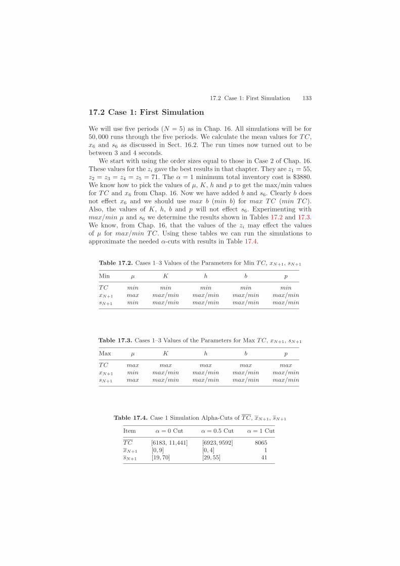
17.2 Case 1: First Simulation 133
17.2 Case 1: First Simulation
We will use five periods (N = 5) as in Chap. 16. All simulations will be for50, 000 runs through the five periods. We calculate the mean values for TC,x6 and s6 as discussed in Sect. 16.2. The run times now turned out to bebetween 3 and 4 seconds.
We start with using the order sizes equal to those in Case 2 of Chap. 16.These values for the zi gave the best results in that chapter. They are z1 = 55,z2 = z3 = z4 = z5 = 71. The α = 1 minimum total inventory cost is $3880.We know how to pick the values of µ, K, h and p to get the max/min valuesfor TC and x6 from Chap. 16. Now we have added b and s6. Clearly b doesnot effect x6 and we should use max b (min b) for max TC (min TC).Also, the values of K, h, b and p will not effect s6. Experimenting withmax/min µ and s6 we determine the results shown in Tables 17.2 and 17.3.We know, from Chap. 16, that the values of the zi may effect the valuesof µ for max/min TC. Using these tables we can run the simulations toapproximate the needed α-cuts with results in Table 17.4.
Table 17.2. Cases 1–3 Values of the Parameters for Min TC, xN+1, sN+1
Min µ K h b p
TC min min min min minxN+1 max max/min max/min max/min max/minsN+1 min max/min max/min max/min max/min
Table 17.3. Cases 1–3 Values of the Parameters for Max TC, xN+1, sN+1
Max µ K h b p
TC max max max max maxxN+1 min max/min max/min max/min max/minsN+1 max max/min max/min max/min max/min
Table 17.4. Case 1 Simulation Alpha-Cuts of TC, xN+1, sN+1
Item α = 0 Cut α = 0.5 Cut α = 1 Cut
TC [6183, 11,441] [6923, 9592] 8065xN+1 [0, 9] [0, 4] 1sN+1 [19, 70] [29, 55] 41

134 17 Inventory Control II
0.8
0 10 20 30 40 50x
1
y
Case 3Case 2
Case 1
Fig. 17.2. Z, τ1 = 3/5, τ2 = 1/5, τ3 = 1/5, in Cases 1, 2, 3
0.8
0 10 20 30 40 50x
1
y
Case 3 Case 1Case 2
Fig. 17.3. Z, τ1 = 1/3, τ2 = 1/3, τ3 = 1/3, in Cases 1, 2, 3
Graphs of the fuzzy goal function Z, for selected values of the τi, areshown in Figs. 17.2–17.4.
17.3 Case 2: Second Simulation
The engineers feel that the value of s6 is too large. A large value of s6 inflatesTC through (17.3). So they agree to increase the zi values to z1 = 61, z2 = 78,z3 = 79, z4 = 80, z5 = 82. The sum of the previous zi values was 339 andthese new zi values add up to 380 an increase of 41. This value of 41 is theα = 1 cut value of s6 in Table 17.4. The α = 1 minimum inventory cost is$4290 which is the cost of buying the items using K = $98.
We know how to choose µ for the max/min x6 and for max/min s6 asshown in Tables 17.2 and 17.3. With these new values of the zi we need toexperiment with the µ values to obtain max/min TC. The final results are

17.4 Case 3: Third Simulation 135
0.8
0 10 20 30 40 50x
1
y
Case 2Case 1Case 3
Fig. 17.4. Z, τ1 = 1/5, τ2 = 2/5, τ3 = 2/5, in Cases 1, 2, 3
the same as those in Tables 17.2 and 17.3. Hence, we may proceed with thesimulation with the alpha-cuts shown in Table 17.5. Now consider the graphsof Z for Case 2 in Figs. 17.2–17.4.
17.4 Case 3: Third Simulation
It now becomes difficult to find zi values to significantly reduce a Z value.Considering the situation were inventory costs are weighted three times ashigh as final inventory (x6) and final lost sales (s6), or τ1 = 3/5, τ2 = τ3 = 1/5in Fig. 17.2, the engineers come up with z1 = 61, z2 = 78, z3 = 77, z4 = 75,z5 = 66. We will now try these values. Their sum is 357 and the cost ofbuying them (K = $98) is 4060. For these new zi values, the values of µfor max/min TC are determined and the results are the same as in Tables17.2–17.3. The simulation results are in Table 17.6.
Table 17.5. Case 2 Simulation Alpha-Cuts of TC, xN+1, sN+1
Item α = 0 Cut α = 0.5 Cut α = 1 Cut
TC [6906, 9061] [7071, 7978] 7365xN+1 [3, 36] [7, 25] 15sN+1 [8, 34] [11, 24] 16
Table 17.6. Case 3 Simulation Alpha-Cuts of TC, xN+1, sN+1
Item α = 0 Cut α = 0.5 Cut α = 1 Cut
TC [6408, 9537] [6674, 8151] 7207xN+1 [0, 19] [1, 10] 4sN+1 [10, 52] [16, 38] 26

136 17 Inventory Control II
17.5 Summary
We see from Figs. 17.2–17.4 that for all cases considered Cases 2 and 3 givealmost identical results and both are better than Case 1. The author triedother choices for the zi values to substantially reduce Z with no success.Maybe the reader can find other amounts to order to obtain a solution betterthan both Case 2 or 3. A GPSS program for one of the simulations in thischapter is in Chap. 28.
Reference
1. J.J. Buckley, T. Feuring and Y. Hayashi: Solving Fuzzy Problems in OperationsResearch: Inventory Control, Soft Computing, 7(2002)121-129. 131

18 Oil Tanker Problem
18.1 Introduction
This model has been adapted from an example in [5]. The system is shownin Fig. 18.1. This figure shows one cycle for an oil tanker. Let us followan oil tanker through one round trip starting at the unload position. Thisunload place is a port on the gulf coast of the US. After unloading the shiptravels to the south Atlantic ocean with travel time T1 in Fig. 18.1. In thischapter unit time is measured in days. T1 will be modelled by the normaldistribution. Once in the south Atlantic the ship may, or may not, experiencea storm, represented as S1. The probability of a storm is p1, so 1 − p1 is theprobability of no storm. A storm causes a delay in the travel time and thisdelay is modelled by the normal distribution. Once out of the south Atlanticit goes around the southern tip of Africa and up the east coast to a port inthe middle east. No storms are to be found there and its travel time is T2also given by the normal distribution. Arriving at port it may, or may not,experience a waiting delay until it can load oil. This possible waiting is codedW1 and the time delay is given by a discrete probability distribution: (1) p10
is the probability of zero wait; (1) p11 the probability of a one day wait; and(3) p12 the probability of a two day wait until docking to load oil.
Unload
S1
T1 T2
W1
W2
T3T4
S2
Load
Fig. 18.1. Oil Tanker Problem
The loading time is given by the normal distribution. Once loaded theship travels back down the east coast of Africa (no storms) with longer traveltime T3 (normal distribution) since it is now full of oil. In the south Atlanticthe probability of a time delay (normal distribution) due to a storm (S2) isp2. Then it travels to the US port for unloading with travel time T4 (normal
James J. Buckley: Simulating Fuzzy Systems, StudFuzz 171, 137–142 (2005)www.springerlink.com c© Springer-Verlag Berlin Heidelberg 2005
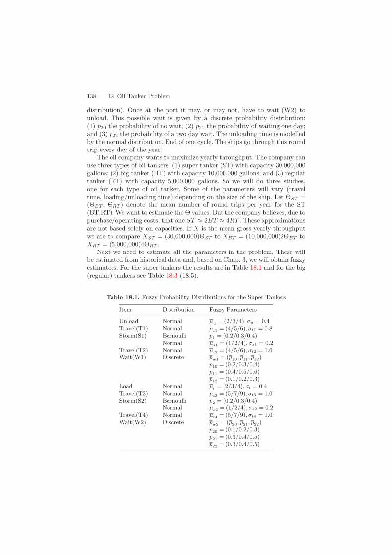
138 18 Oil Tanker Problem
distribution). Once at the port it may, or may not, have to wait (W2) tounload. This possible wait is given by a discrete probability distribution:(1) p20 the probability of no wait; (2) p21 the probability of waiting one day;and (3) p22 the probability of a two day wait. The unloading time is modelledby the normal distribution. End of one cycle. The ships go through this roundtrip every day of the year.
The oil company wants to maximize yearly throughput. The company canuse three types of oil tankers: (1) super tanker (ST) with capacity 30,000,000gallons; (2) big tanker (BT) with capacity 10,000,000 gallons; and (3) regulartanker (RT) with capacity 5,000,000 gallons. So we will do three studies,one for each type of oil tanker. Some of the parameters will vary (traveltime, loading/unloading time) depending on the size of the ship. Let ΘST =(ΘBT , ΘRT ) denote the mean number of round trips per year for the ST(BT,RT). We want to estimate the Θ values. But the company believes, due topurchase/operating costs, that one ST ≈ 2BT ≈ 4RT . These approximationsare not based solely on capacities. If X is the mean gross yearly throughputwe are to compare XST = (30,000,000)ΘST to XBT = (10,000,000)2ΘBT toXRT = (5,000,000)4ΘRT .
Next we need to estimate all the parameters in the problem. These willbe estimated from historical data and, based on Chap. 3, we will obtain fuzzyestimators. For the super tankers the results are in Table 18.1 and for the big(regular) tankers see Table 18.3 (18.5).
Table 18.1. Fuzzy Probability Distributions for the Super Tankers
Item Distribution Fuzzy Parameters
Unload Normal µu = (2/3/4), σu = 0.4Travel(T1) Normal µt1 = (4/5/6), σt1 = 0.8Storm(S1) Bernoulli p1 = (0.2/0.3/0.4)
Normal µs1 = (1/2/4), σs1 = 0.2Travel(T2) Normal µt2 = (4/5/6), σt2 = 1.0Wait(W1) Discrete pw1 = (p10, p11, p12)
p10 = (0.2/0.3/0.4)p11 = (0.4/0.5/0.6)p12 = (0.1/0.2/0.3)
Load Normal µl = (2/3/4), σl = 0.4Travel(T3) Normal µt3 = (5/7/9), σt3 = 1.0Storm(S2) Bernoulli p2 = (0.2/0.3/0.4)
Normal µs2 = (1/2/4), σs2 = 0.2Travel(T4) Normal µt4 = (5/7/9), σt4 = 1.0Wait(W2) Discrete pw2 = (p20, p21, p22)
p20 = (0.1/0.2/0.3)p21 = (0.3/0.4/0.5)p22 = (0.3/0.4/0.5)

18.3 Case 2: Big Tankers 139
We assume that there is a continuous function FST (all parameters) =XST so that by the extension principle XST = FST (fuzzy parameters).Then, from Chap. 7, we may employ crisp simulation to estimate α-cuts ofXST . We make the same assumptions for XBT and XRT . However, we donot know the structure of these one-step functions. Hence, we proceed tothe crisp simulation. The goal is to estimate and compare the three fuzzynumbers XST , XBT , XRT . These fuzzy numbers are easily found from thefuzzy numbers ΘST , ΘBT , ΘRT which will be estimated from simulation.
18.2 Case 1: Super Tankers
For the super tanker the fuzzy probability distributions are shown inTable 18.1. Now we need to figure out how to choose the values of the µu,µt1, . . . , p22 in their α-cuts to estimate the end points of the intervals for theα-cuts of ΘST . It is fairly obvious that for maxΘ (minΘ) we use the minimum(maximum) of µu, µt1, p1, µs1, µt2, µl, µt3, p2, µs2, and µt4. However, the pij ,i = 1, 2, j = 0, 1, 2 in Table 18.1 are different. We may choose pij ∈ pij [α] butwe must have a discrete probability distribution pi0 + pi1 + pi2 = 1, i = 1, 2[1, 2, 3, 4]. So for maxΘ (minΘ) and i = 1 we first pick maxp10 (minp10)if possible, then maxp11 (minp11) if possible, and then maxp12 (minp12) ifpossible. The “if possible” means that you need to pick all three probabilitiesso that their sum is one. Similarly, choose the p2j , j = 0, 1, 2. For example,suppose p10[0] = [0.1, 0.4], p11[0] = [0.3, 0.6] and p12[0] = [0.2, 0.5]. Then formaxΘ pick p10 = 0.4, p11 = 0.4, p12 = 0.2. We can not use p11 = 0.6 becausethe smallest value for p12 is 0.2.
Using these results we may now do the simulations. All simulations werefor 50,000 round trips. For one simulation run of 50,000 cycles CLOCK =total days in the simulation so ΘST = [50,000]/[CLOCK/365]. Each simula-tion run averaged around two seconds. The results for the super tankers arein Table 18.2.
We show the graphs of Θ in Fig. 18.2 followed by the graphs of the X inFig. 18.3.
18.3 Case 2: Big Tankers
The big tankers load/unload and travel faster than the super tankers. Thismeans that the values of µu, µt1, µt2, µl, µt3 and µt4 are all smaller for a BT
Table 18.2. Case 1 Simulation Alpha-Cuts of ΘST
Item α = 0 Cut α = 0.5 Cut α = 1 Cut
ΘST [8.35, 15.14] [9.50, 12.73] 10.96

140 18 Oil Tanker Problem
0.8
0 5 10 15 20 25x
1
yΘRTΘBTΘST
Fig. 18.2. Θ (Trips/Year) in Cases 1–3
0.8
0 10 20 30 40 50x
1
y
XRT
XBT XST
Fig. 18.3. X (Gals./Year) in Cases 1–3, Scale = x(10)7 gals
than for a ST. The values of the fuzzy parameters for the big tankers are inTable 18.3. The values that do not change from Table 18.1 to Table 18.3 arethose of p1, µs1, σs1, pw1, p2, µs2, σs2 and pw2. Simulation results are shownin Table 18.4 with graphs in Figs. 18.2 and 18.3.
18.4 Case 3: Regular Tankers
Regular tankers load/unload and travel faster than big tankers. The values ofthe fuzzy parameters for regular tankers are in Table 18.5. Some values havebeen decreased while others are unchanged. The changes from Table 18.3 to18.5 are similar to those from Table 18.1 to 18.3. Simulation results are givenin Table 18.6 with graphs in Figs. 18.2 and 18.3.
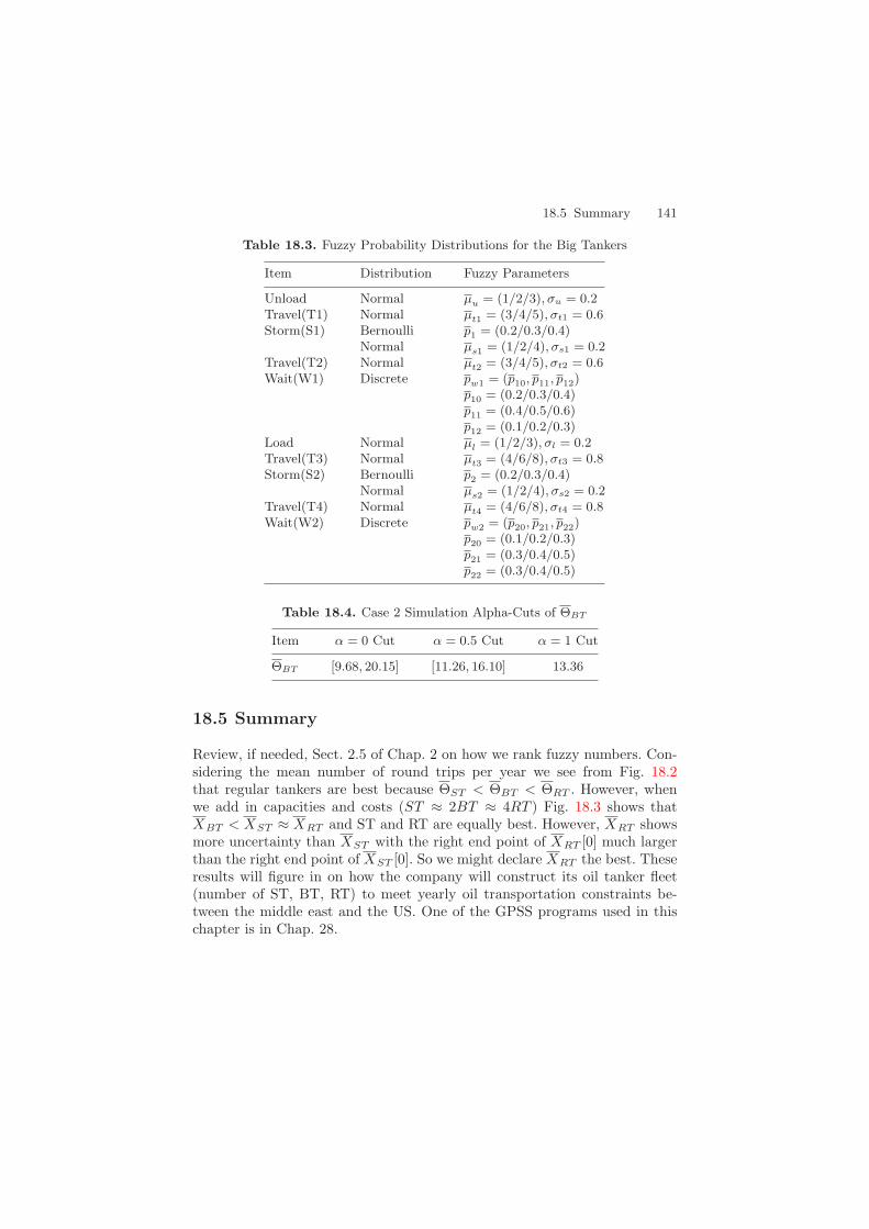
18.5 Summary 141
Table 18.3. Fuzzy Probability Distributions for the Big Tankers
Item Distribution Fuzzy Parameters
Unload Normal µu = (1/2/3), σu = 0.2Travel(T1) Normal µt1 = (3/4/5), σt1 = 0.6Storm(S1) Bernoulli p1 = (0.2/0.3/0.4)
Normal µs1 = (1/2/4), σs1 = 0.2Travel(T2) Normal µt2 = (3/4/5), σt2 = 0.6Wait(W1) Discrete pw1 = (p10, p11, p12)
p10 = (0.2/0.3/0.4)p11 = (0.4/0.5/0.6)p12 = (0.1/0.2/0.3)
Load Normal µl = (1/2/3), σl = 0.2Travel(T3) Normal µt3 = (4/6/8), σt3 = 0.8Storm(S2) Bernoulli p2 = (0.2/0.3/0.4)
Normal µs2 = (1/2/4), σs2 = 0.2Travel(T4) Normal µt4 = (4/6/8), σt4 = 0.8Wait(W2) Discrete pw2 = (p20, p21, p22)
p20 = (0.1/0.2/0.3)p21 = (0.3/0.4/0.5)p22 = (0.3/0.4/0.5)
Table 18.4. Case 2 Simulation Alpha-Cuts of ΘBT
Item α = 0 Cut α = 0.5 Cut α = 1 Cut
ΘBT [9.68, 20.15] [11.26, 16.10] 13.36
18.5 Summary
Review, if needed, Sect. 2.5 of Chap. 2 on how we rank fuzzy numbers. Con-sidering the mean number of round trips per year we see from Fig. 18.2that regular tankers are best because ΘST < ΘBT < ΘRT . However, whenwe add in capacities and costs (ST ≈ 2BT ≈ 4RT ) Fig. 18.3 shows thatXBT < XST ≈ XRT and ST and RT are equally best. However, XRT showsmore uncertainty than XST with the right end point of XRT [0] much largerthan the right end point of XST [0]. So we might declare XRT the best. Theseresults will figure in on how the company will construct its oil tanker fleet(number of ST, BT, RT) to meet yearly oil transportation constraints be-tween the middle east and the US. One of the GPSS programs used in thischapter is in Chap. 28.

142 18 Oil Tanker Problem
Table 18.5. Fuzzy Probability Distributions for the Regular Tankers
Item Distribution Fuzzy Parameters
Unload Normal µu = (0.5/1/1.5), σu = 0.1Travel(T1) Normal µt1 = (2/3/4), σt1 = 0.4Storm(S1) Bernoulli p1 = (0.2/0.3/0.4)
Normal µs1 = (1/2/4), σs1 = 0.2Travel(T2) Normal µt2 = (2/3/4), σt2 = 0.4Wait(W1) Discrete pw1 = (p10, p11, p12)
p10 = (0.2/0.3/0.4)p11 = (0.4/0.5/0.6)p12 = (0.1/0.2/0.3)
Load Normal µl = (0.5/1/1.5), σl = 0.1Travel(T3) Normal µt3 = (3/5/7), σt3 = 0.6Storm(S2) Bernoulli p2 = (0.2/0.3/0.4)
Normal µs2 = (1/2/4), σs2 = 0.2Travel(T4) Normal µt4 = (3/5/7), σt4 = 0.6Wait(W2) Discrete pw2 = (p20, p21, p22)
p20 = (0.1/0.2/0.3)p21 = (0.3/0.4/0.5)p22 = (0.3/0.4/0.5)
Table 18.6. Case 3 Simulation Alpha-Cuts of ΘRT
Item α = 0 Cut α = 0.5 Cut α = 1 Cut
ΘRT [11.89, 27.84] [14.09, 21.26] 17.12
References
1. J.J. Buckley: Fuzzy Probabilities: New Approach and Applications,Physica-Verlag, Heidelberg, Germany, 2003. 139
2. J.J. Buckley: Fuzzy Probabilities and Fuzzy Sets for Web Planning, Springer,Heidelberg, Germany, 2004. 139
3. J.J. Buckley and E. Eslami: Uncertain Probabilities I: The Discrete Case, SoftComputing, 7(2003)500-505. 139
4. J.J. Buckley, K. Reilly and X. Zheng: Fuzzy Probabilities for Web Planning,Soft Computing, 8(2004)464-476. 139
5. Thomas J. Schriber: Simulation Using GPSS, John Wiley and Sons, New York,1974. 137

19 Priority Queues
19.1 Introduction
This chapter will use the queuing system in Chaps. 5 and 9, but with pri-ority orders. The system is shown in Fig. 19.1. Everything is the same as inFig. 5.1 (9.1) except for the arrivals. Now we have three types of arrivals: (1)lowest level is called Priority #1; (2) the next lowest level is Priority #2; and(3) the highest level is labelled Priority #3. Priority determines how an itemis handled in a queue. In any queue all items with priority #3 go to the frontof the queue and are serviced on a first come, first served, basis. If there areno Priority #3 items in the queue, then all those with Priority #2 go to thefront of the queue and are serviced in a first come, first served, manner. Allitems of Priority #1 are serviced in the first come, first served, mode if thereare no Priority #2 or #3 items in the queue. There are different prioritylevels because we have different types of customers. The highest priority isgiven to those customers who pay in cash, so there are no billing expenses,and they place many orders. Similarly, we determine the other priority levels.
The rest of the system in Fig. 19.1 is as described in Chap. 5 (9), butwe have made changes in some of the probability distributions. Arrivals aremodelled using the uniform distribution and all service stations will use thenormal distribution for service time. We estimate all parameters from his-torical data on the system, so we will obtain as in Chap. 3 fuzzy estimators.Hence, we have the fuzzy uniform (Chap. 4) for arrivals and the fuzzy nor-mal (Chap. 4) for service time. All these fuzzy distributions are defined inTable 19.1. We also assume that all queues have unlimited capacity as as-sumed in Chap. 9.
The time unit in this chapter is one hour. All simulations, unless statedotherwise, will be until there are 50,000 itemsin the Accept-Finished box (theswamping method in Chap. 7). At the end of a simulation CLOCK will havethe total hours in the study. Considering a work day to last eight hours,then CLOCK/8 gives the number of days in the simulation. Managementis interested in finding R = mean time an item spends in the system andX = expected number of Accepted-Finished units per day. Let Ri(Xi) bethe value of R(X) for Priority #i orders, i = 1, 2, 3. We may find the Ri
from the standard output file in the simulation. But the standard output filecan be made to give TXi = the total Priority #i items that ended up in
James J. Buckley: Simulating Fuzzy Systems, StudFuzz 171, 143–148 (2005)www.springerlink.com c© Springer-Verlag Berlin Heidelberg 2005

144 19 Priority Queues
Priority 1
Priority 2
Priority 3
Arrive
Q1
S1 Q2
S21
S22
Q3
S3 Q4
S41
S42
S43
Q5
S51
S52
Accept-Finished
Reject
1 − p
p
Fig. 19.1. Priority Queuing System
Table 19.1. Fuzzy Probability Distributions for Fig. 19.1
Item Distribution Details
Priority 1 Uniform a1 = (0.15/0.20/0.25),b1 = (0.35/0.40/0.45)
Priority 2 Uniform a2 = (0.25/0.30/0.35),b2 = (0.45/0.50/0.55)
Priority 3 Uniform a3 = (0.35/0.40/0.45),b3 = (0.55/0.60/0.65)Server = S1 Normal µ1 = (0.06/0.08/0.10), σ1 = 0.012Servers = S2 Normal µ2 = (0.1/0.15/0.2), σ2 = 0.02Server = S3 Normal µ3 = (0.06/0.08/0.10).σ3 = 0.012Servers = S4 Normal µ4 = (0.1/0.15/0.2), σ4 = 0.02Server = S51 Normal µ51 = (0.05/0.1/0.15), σ51 = 0.01Server = S52 Normal µ52 = (0.15/0.20/0.25), σ52 = 0.03Transfer Bernoulli p = (0.03/0.05/0.07)
the Accept-Finished box, i = 1, 2, 3, for a total of 50,000 units in that box.Therefore, Xi = TXi/[CLOCK/8], i = 1, 2, 3.
We assume that there are continuous functions Fi (Gi) so thatRi = Fi(all parameters) (Xi = Gi(all parameters)), i = 1, 2, 3. By theextension principle (Chap. 2) we obtain Ri = Fi(fuzzy parameters) (Xi =G(fuzzy parameters)), i = 1, 2, 3. However, these functions are not availableto us. Therefore, we use crisp simulation to estimate the α-cuts of the Ri andthe Xi (Chap. 7).
Next we need to determine how to pick a1 ∈ a1[α], b1 ∈ b1[α], . . . , p ∈ p[α]to approximate the end points of the intervals for Rk[α] and Xk[α]. From

19.1 Introduction 145
Table 19.2. Values of the Parameters for Min Xk, Rk, k = 1, 2, 3
Min ai bi µj p
Xk max max max/min maxRk max max min any
Table 19.3. Values of the Parameters for Max Xk, Rk, k = 1, 2, 3
Max ai bi µj p
Xk min min max/min minRk min min max any
previous experience, plus some experimenting, the results are inTables 19.2 and 19.3. Let us explain how we are going to use these tables.First assume that we wish to estimate the left end point of Rk[α], k = 1, 2, 3.Table 19.2 implies that in the simulation use: (1) ai the right end point ofai[α], i = 1, 2, 3; (2) bi the right end point of bi[α], i = 1, 2, 3; (3) µj theleft end point of µj [α], j = 1, 2, 3, 4, 51, 52; and (4) p any value in p[α]. Nextconsider using simulation to estimate the right end point of Xk[α], k = 1, 2, 3.Table 19.3 says to use: (1) ai the left end point of ai[α], i = 1, 2, 3; (2) bi
the left end point of bi[α], i = 1, 2, 3; (3) µj the left, or right, end point ofµj [α], j = 1, 2, 3, 4, 51, 52; and (4) p the left end point of p[α]. We found thatyou get essentially the same results for max/minXk using minµj or maxµj ,k = 1, 2, 3, j = 1, 2, 3, 4, 51, 52.
Management wants to minimize the Ri with minimizing R3 more impor-tant than minimizing the other two. Management also states that they wouldlike to maximize the Xi with preference on maximizing X3 first, then X2 andX1 last. Let
Zr = τ11R1 + τ12R2 + τ13R3 , (19.1)
andZx = τ21X1 + τ22X2 + τ23X3 , (19.2)
for τij > 0,∑3
j=1 τij = 1, i = 1, 2. So we want to minZr and maxZx. LetM > 0 be sufficiently large so that minZr is equivalent to max[M − Zr].Finally we want to maxZ where
Z = κ1[M − Zr] + κ2Zx , (19.3)
for κi > 0 and κ1 +κ2 = 1. We decide on τ11 = 1/6, τ12 = 2/6, τ13 = 3/6 andτ21 = 1/6, τ22 = 2/6, τ23 = 3/6. We will use M = 10 and κ1 = 1/3, κ2 = 2/3.These are the values that we will use in this chapter to compute Z in thesimulations. The emphasis was placed on Priority #3 first, then Priority#2 and lastly Priority #1 customers and on throughput X over responsetime R.
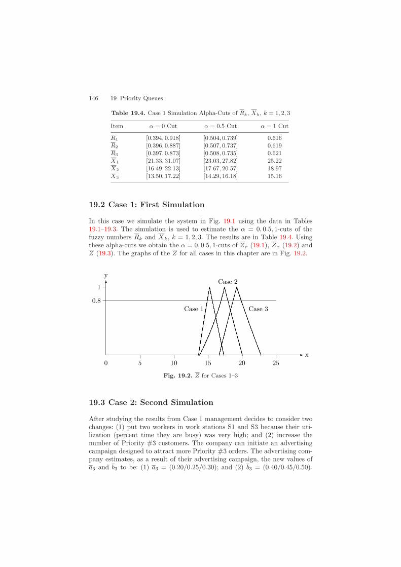
146 19 Priority Queues
Table 19.4. Case 1 Simulation Alpha-Cuts of Rk, Xk, k = 1, 2, 3
Item α = 0 Cut α = 0.5 Cut α = 1 Cut
R1 [0.394, 0.918] [0.504, 0.739] 0.616
R2 [0.396, 0.887] [0.507, 0.737] 0.619
R3 [0.397, 0.873] [0.508, 0.735] 0.621
X1 [21.33, 31.07] [23.03, 27.82] 25.22
X2 [16.49, 22.13] [17.67, 20.57] 18.97
X3 [13.50, 17.22] [14.29, 16.18] 15.16
19.2 Case 1: First Simulation
In this case we simulate the system in Fig. 19.1 using the data in Tables19.1–19.3. The simulation is used to estimate the α = 0, 0.5, 1-cuts of thefuzzy numbers Rk and Xk, k = 1, 2, 3. The results are in Table 19.4. Usingthese alpha-cuts we obtain the α = 0, 0.5, 1-cuts of Zr (19.1), Zx (19.2) andZ (19.3). The graphs of the Z for all cases in this chapter are in Fig. 19.2.
0.8
0 5 10 15 20 25x
1
y
Case 1 Case 3
Case 2
Fig. 19.2. Z for Cases 1–3
19.3 Case 2: Second Simulation
After studying the results from Case 1 management decides to consider twochanges: (1) put two workers in work stations S1 and S3 because their uti-lization (percent time they are busy) was very high; and (2) increase thenumber of Priority #3 customers. The company can initiate an advertisingcampaign designed to attract more Priority #3 orders. The advertising com-pany estimates, as a result of their advertising campaign, the new values ofa3 and b3 to be: (1) a3 = (0.20/0.25/0.30); and (2) b3 = (0.40/0.45/0.50).
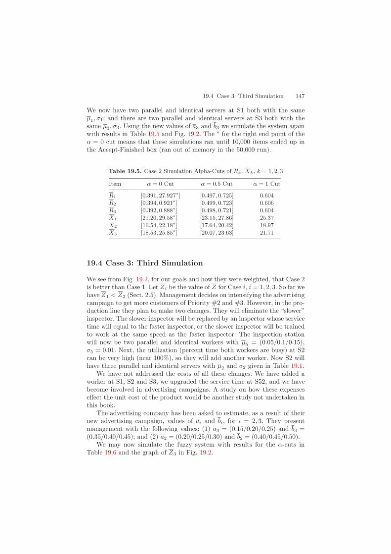
19.4 Case 3: Third Simulation 147
We now have two parallel and identical servers at S1 both with the sameµ1, σ1; and there are two parallel and identical servers at S3 both with thesame µ3, σ3. Using the new values of a3 and b3 we simulate the system againwith results in Table 19.5 and Fig. 19.2. The ∗ for the right end point of theα = 0 cut means that these simulations ran until 10,000 items ended up inthe Accept-Finished box (ran out of memory in the 50,000 run).
Table 19.5. Case 2 Simulation Alpha-Cuts of Rk, Xk, k = 1, 2, 3
Item α = 0 Cut α = 0.5 Cut α = 1 Cut
R1 [0.391, 27.927∗] [0.497, 0.725] 0.604
R2 [0.394, 0.921∗] [0.499, 0.723] 0.606
R3 [0.392, 0.888∗] [0.498, 0.721] 0.604
X1 [21.20, 29.58∗] [23.15, 27.86] 25.37
X2 [16.54, 22.18∗] [17.64, 20.42] 18.97
X3 [18.53, 25.85∗] [20.07, 23.63] 21.71
19.4 Case 3: Third Simulation
We see from Fig. 19.2, for our goals and how they were weighted, that Case 2is better than Case 1. Let Zi be the value of Z for Case i, i = 1, 2, 3. So far wehave Z1 < Z2 (Sect. 2.5). Management decides on intensifying the advertisingcampaign to get more customers of Priority #2 and #3. However, in the pro-duction line they plan to make two changes. They will eliminate the “slower”inspector. The slower inspector will be replaced by an inspector whose servicetime will equal to the faster inspector, or the slower inspector will be trainedto work at the same speed as the faster inspector. The inspection stationwill now be two parallel and identical workers with µ5 = (0.05/0.1/0.15),σ5 = 0.01. Next, the utilization (percent time both workers are busy) at S2can be very high (near 100%), so they will add another worker. Now S2 willhave three parallel and identical servers with µ2 and σ2 given in Table 19.1.
We have not addressed the costs of all these changes. We have added aworker at S1, S2 and S3, we upgraded the service time at S52, and we havebecome involved in advertising campaigns. A study on how these expenseseffect the unit cost of the product would be another study not undertaken inthis book.
The advertising company has been asked to estimate, as a result of theirnew advertising campaign, values of ai and bi, for i = 2, 3. They presentmanagement with the following values: (1) a3 = (0.15/0.20/0.25) and b3 =(0.35/0.40/0.45); and (2) a2 = (0.20/0.25/0.30) and b2 = (0.40/0.45/0.50).
We may now simulate the fuzzy system with results for the α-cuts inTable 19.6 and the graph of Z3 in Fig. 19.2.
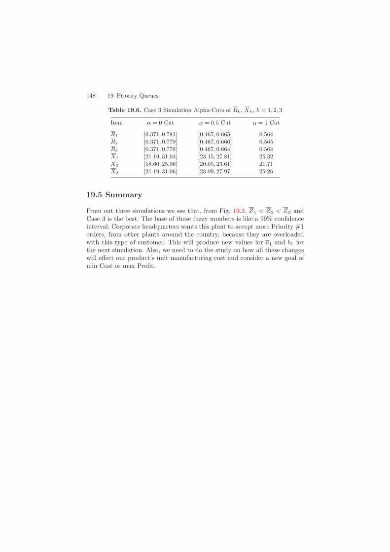
148 19 Priority Queues
Table 19.6. Case 3 Simulation Alpha-Cuts of Rk, Xk, k = 1, 2, 3
Item α = 0 Cut α = 0.5 Cut α = 1 Cut
R1 [0.371, 0.781] [0.467, 0.665] 0.564
R2 [0.371, 0.779] [0.467, 0.666] 0.565
R3 [0.371, 0.778] [0.467, 0.664] 0.564
X1 [21.19, 31.04] [23.15, 27.81] 25.32
X2 [18.60, 25.96] [20.05, 23.61] 21.71
X3 [21.19, 31.06] [23.09, 27.97] 25.26
19.5 Summary
From out three simulations we see that, from Fig. 19.2, Z1 < Z2 < Z3 andCase 3 is the best. The base of these fuzzy numbers is like a 99% confidenceinterval. Corporate headquarters wants this plant to accept more Priority #1orders, from other plants around the country, because they are overloadedwith this type of customer. This will produce new values for a1 and b1 forthe next simulation. Also, we need to do the study on how all these changeswill effect our product’s unit manufacturing cost and consider a new goal ofmin Cost or max Profit.
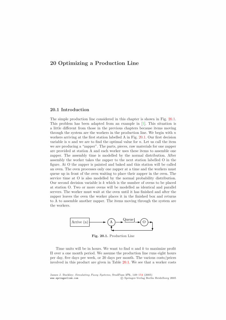
20 Optimizing a Production Line
20.1 Introduction
The simple production line considered in this chapter is shown in Fig. 20.1.This problem has been adapted from an example in [1]. This situation isa little different from those in the previous chapters because items movingthrough the system are the workers in the production line. We begin with nworkers arriving at the first station labelled A in Fig. 20.1. Our first decisionvariable is n and we are to find the optimal value for n. Let us call the itemwe are producing a “zapper”. The parts, pieces, raw materials for one zapperare provided at station A and each worker uses these items to assemble onezapper. The assembly time is modelled by the normal distribution. Afterassembly the worker takes the zapper to the next station labelled O in thefigure. At O the zapper is painted and baked and this station will be calledan oven. The oven processes only one zapper at a time and the workers mustqueue up in front of the oven waiting to place their zapper in the oven. Theservice time at O is also modelled by the normal probability distribution.Our second decision variable is k which is the number of ovens to be placedat station O. Two or more ovens will be modelled as identical and parallelservers. The worker must wait at the oven until it has finished and after thezapper leaves the oven the worker places it in the finished box and returnsto A to assemble another zapper. The items moving through the system arethe workers.
Arrive (n)
A Queue
O
Fig. 20.1. Production Line
Time units will be in hours. We want to find n and k to maximize profitΠ over a one month period. We assume the production line runs eight hoursper day, five days per week, or 20 days per month. The various costs/pricesinvolved in this product are given in Table 20.1. We see that a worker costs
James J. Buckley: Simulating Fuzzy Systems, StudFuzz 171, 149–154 (2005)www.springerlink.com c© Springer-Verlag Berlin Heidelberg 2005
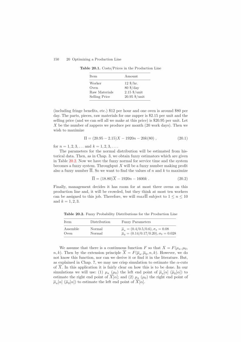
150 20 Optimizing a Production Line
Table 20.1. Costs/Prices in the Production Line
Item Amount
Worker 12 $/hr.Oven 80 $/dayRaw Materials 2.15 $/unitSelling Price 20.95 $/unit
(including fringe benefits, etc.) $12 per hour and one oven is around $80 perday. The parts, pieces, raw materials for one zapper is $2.15 per unit and theselling price (and we can sell all we make at this price) is $20.95 per unit. LetX be the number of zappers we produce per month (20 work days). Then wewish to maximize
Π = (20.95 − 2.15)X − 1920n − 20k(80) , (20.1)
for n = 1, 2, 3, . . . and k = 1, 2, 3, . . . .The parameters for the normal distribution will be estimated from his-
torical data. Then, as in Chap. 3, we obtain fuzzy estimators which are givenin Table 20.2. Now we have the fuzzy normal for service time and the systembecomes a fuzzy system. Throughput X will be a fuzzy number making profitalso a fuzzy number Π. So we want to find the values of n and k to maximize
Π = (18.80)X − 1920n − 1600k . (20.2)
Finally, management decides it has room for at most three ovens on thisproduction line and, it will be crowded, but they think at most ten workerscan be assigned to this job. Therefore, we will maxΠ subject to 1 ≤ n ≤ 10and k = 1, 2, 3.
Table 20.2. Fuzzy Probability Distributions for the Production Line
Item Distribution Fuzzy Parameters
Assemble Normal µa = (0.4/0.5/0.6), σa = 0.08Oven Normal µ0 = (0.14/0.17/0.20), σ0 = 0.028
We assume that there is a continuous function F so that X = F (µa, µ0,n, k). Then by the extension principle X = F (µa, µ0, n, k). However, we donot know this function, nor can we derive it or find it in the literature. But,as explained in Chap. 7, we may use crisp simulation to estimate the α-cutsof X. In this application it is fairly clear on how this is to be done. In oursimulations we will use: (1) µa (µ0) the left end point of µa[α] (µ0[α]) toestimate the right end point of X[α]; and (2) µa (µ0) the right end point ofµa[α] (µ0[α]) to estimate the left end point of X[α].
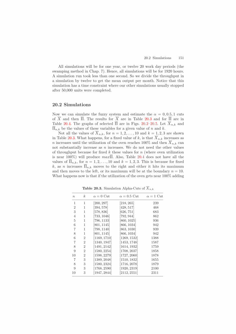
20.2 Simulations 151
All simulations will be for one year, or twelve 20 work day periods (theswamping method in Chap. 7). Hence, all simulations will be for 1920 hours.A simulation run took less than one second. So we divide the throughput ina simulation by twelve to get the mean output per month. Notice that thissimulation has a time constraint where our other simulations usually stoppedafter 50,000 units were completed.
20.2 Simulations
Now we can simulate the fuzzy system and estimate the α = 0, 0.5, 1 cutsof X and then Π. The results for X are in Table 20.3 and for Π are inTable 20.4. The graphs of selected Π are in Figs. 20.2–20.5. Let Xn,k andΠn,k be the values of these variables for a given value of n and k.
Not all the values of Xn,k, for n = 1, 2, . . . , 10 and k = 1, 2, 3 are shownin Table 20.3. What happens, for a fixed value of k, is that Xn,k increases asn increases until the utilization of the oven reaches 100% and then Xn,k cannot substantially increase as n increases. We do not need the other valuesof throughput because for fixed k these values for n (where oven utilizationis near 100%) will produce maxΠ. Also, Table 20.4 does not have all thevalues of Πn,k, for n = 1, 2, . . . , 10 and k = 1, 2, 3. This is because for fixedk, as n increases Πn,k moves to the right and either it hits its maximumand then moves to the left, or its maximum will be at the boundary n = 10.What happens now is that if the utilization of the oven gets near 100% adding
Table 20.3. Simulation Alpha-Cuts of Xn,k
n k α = 0 Cut α = 0.5 Cut α = 1 Cut
1 1 [200, 297] [218, 265] 2392 1 [394, 578] [428, 517] 4683 1 [578, 836] [626, 751] 6834 1 [733, 1046] [792, 944] 8625 1 [796, 1133] [860, 1025] 9366 1 [801, 1145] [866, 1034] 9427 1 [798, 1140] [863, 1030] 9398 1 [801, 1145] [866, 1034] 9426 2 [1169, 1710] [1269, 1532] 13887 2 [1340, 1947] [1453, 1748] 15878 2 [1491, 2142] [1614, 1932] 17599 2 [1580, 2254] [1708, 2037] 1858
10 2 [1598, 2279] [1727, 2060] 18787 3 [1389, 2048] [1510, 1832] 16558 3 [1580, 2324] [1716, 2078] 18799 3 [1768, 2590] [1920, 2319] 2100
10 3 [1947, 2844] [2112, 2551] 2311
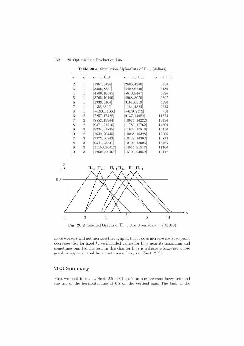
152 20 Optimizing a Production Line
Table 20.4. Simulation Alpha-Cuts of Πn,k (dollars)
n k α = 0 Cut α = 0.5 Cut α = 1 Cut
2 1 [1967, 5426] [2606, 4280] 33583 1 [3506, 8357] [4409, 6759] 54804 1 [4500, 10385] [5610, 8467] 69265 1 [3765, 10100] [4968, 8070] 63976 1 [1939, 8406] [3161, 6319] 45907 1 [−38, 6392] [1184, 4324] 26138 1 [−1901, 4566] [−679, 2479] 7506 2 [7257, 17428] [9137, 14082] 113747 2 [8552, 19964] [10676, 16222] 131968 2 [9471, 21710] [11783, 17762] 145099 2 [9224, 21895] [11630, 17816] 14450
10 2 [7642, 20445] [10068, 16328] 129067 3 [7873, 20262] [10148, 16202] 128748 3 [9544, 23531] [12101, 18906] 151659 3 [11158, 26612] [14016, 21517] 17400
10 3 [12604, 29467] [15706, 23959] 19447
0.8
0 2 4 6 8 10x
1
yΠ4,1Π3,1Π7,1 Π6,1Π2,1 Π5,1
Fig. 20.2. Selected Graphs of Πn,1, One Oven, scale = x($1000)
more workers will not increase throughput, but it does increase costs, so profitdecreases. So, for fixed k, we included values for Πn,k near its maximum andsometimes omitted the rest. In this chapter Πn,k is a discrete fuzzy set whosegraph is approximated by a continuous fuzzy set (Sect. 2.7).
20.3 Summary
First we need to review Sect. 2.5 of Chap. 2 on how we rank fuzzy sets andthe use of the horizontal line at 0.8 on the vertical axis. The base of the
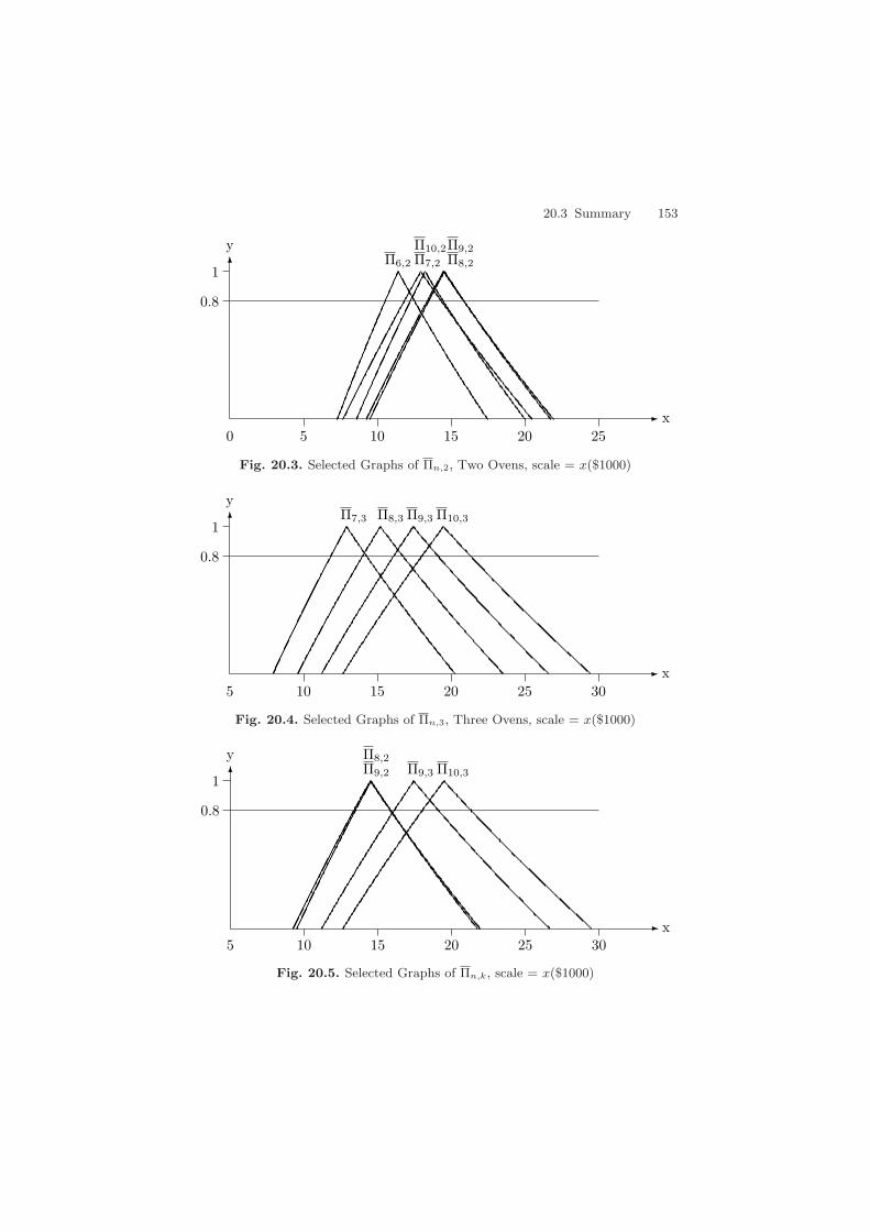
20.3 Summary 153
0.8
0 5 10 15 20 25x
1
yΠ7,2Π6,2 Π8,2
Π10,2Π9,2
Fig. 20.3. Selected Graphs of Πn,2, Two Ovens, scale = x($1000)
0.8
5 10 15 20 25 30x
1
yΠ7,3 Π8,3 Π9,3 Π10,3
Fig. 20.4. Selected Graphs of Πn,3, Three Ovens, scale = x($1000)
0.8
5 10 15 20 25 30x
1
yΠ9,2
Π8,2Π9,3 Π10,3
Fig. 20.5. Selected Graphs of Πn,k, scale = x($1000)

154 20 Optimizing a Production Line
fuzzy numbers in Figs. 20.2–20.4 are like 99% confidence intervals. If thereis only one oven Fig. 20.2 shows that: (1) Π5,1 ≈ Π4,1 and Π4,1 > Πn,1 forn = 2, 3, 6, 7. Using two ovens Fig. 20.3 implies that: (1) Π7,2 ≈ Π8,2 ≈ Π9,2 ≈Π10,2; and (2) Π8,2, Π9,2 > Π6,2. For three ovens (k = 3) Fig. 20.4 says that:(1) Π9,3 ≈ Π10,3; and (2) Π10,3 > Π8,3, Π7,3. It is obvious that Π10,3 > Πn,1
for n = 1, 2, 3, . . . , 10. Figure 20.5 compares the largest values for k = 2 andk = 3 giving our final conclusion: (1) Π10,3 ≈ Π9,3; and (2) Π10,3 > Πn,2,for n = 1, 2, 3, . . . , 10. We maximize profit by loading up the production linewith the maximum number of workers and ovens.
Reference
1. Thomas J. Schriber: Simulation Using GPSS, John Wiley and Sons, New York,1974. 149
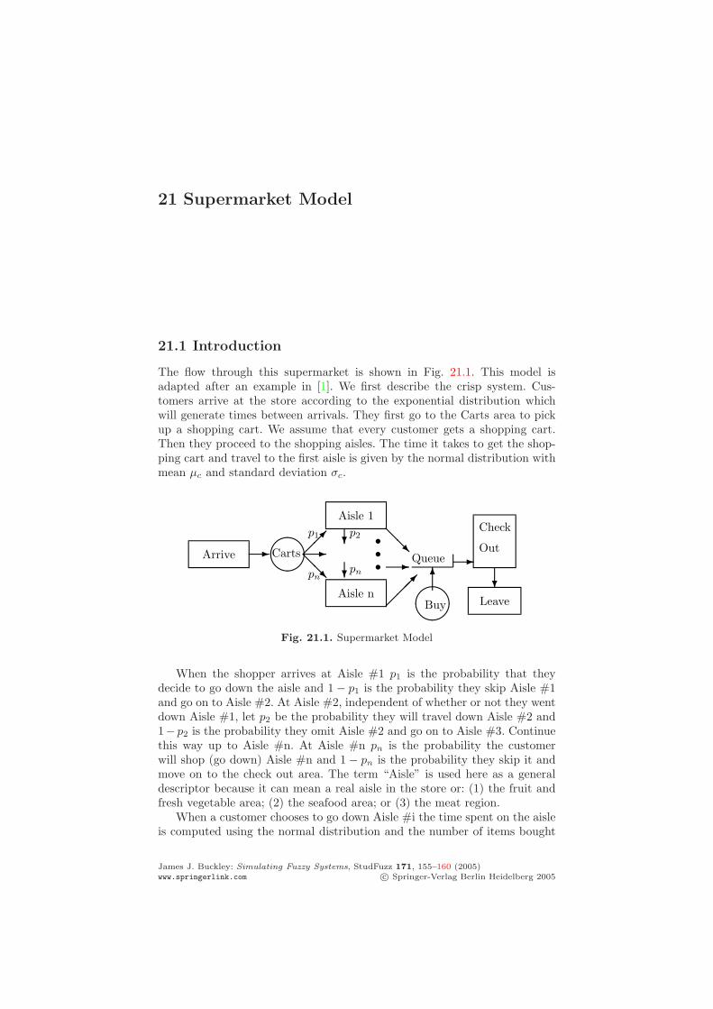
21 Supermarket Model
21.1 Introduction
The flow through this supermarket is shown in Fig. 21.1. This model isadapted after an example in [1]. We first describe the crisp system. Cus-tomers arrive at the store according to the exponential distribution whichwill generate times between arrivals. They first go to the Carts area to pickup a shopping cart. We assume that every customer gets a shopping cart.Then they proceed to the shopping aisles. The time it takes to get the shop-ping cart and travel to the first aisle is given by the normal distribution withmean µc and standard deviation σc.
Arrive
Carts
Aisle 1p1
pn
p2
pn
Aisle n
Queue
Buy
Check
Out
Leave
Fig. 21.1. Supermarket Model
When the shopper arrives at Aisle #1 p1 is the probability that theydecide to go down the aisle and 1 − p1 is the probability they skip Aisle #1and go on to Aisle #2. At Aisle #2, independent of whether or not they wentdown Aisle #1, let p2 be the probability they will travel down Aisle #2 and1− p2 is the probability they omit Aisle #2 and go on to Aisle #3. Continuethis way up to Aisle #n. At Aisle #n pn is the probability the customerwill shop (go down) Aisle #n and 1 − pn is the probability they skip it andmove on to the check out area. The term “Aisle” is used here as a generaldescriptor because it can mean a real aisle in the store or: (1) the fruit andfresh vegetable area; (2) the seafood area; or (3) the meat region.
When a customer chooses to go down Aisle #i the time spent on the aisleis computed using the normal distribution and the number of items bought
James J. Buckley: Simulating Fuzzy Systems, StudFuzz 171, 155–160 (2005)www.springerlink.com c© Springer-Verlag Berlin Heidelberg 2005

156 21 Supermarket Model
(put into the shopping cart) is given by a discrete probability distributionPROBi, 1 ≤ i ≤ m. This normal distribution has mean µi and standarddeviation σi, 1 ≤ i ≤ n.
The check out area has one, two, or three check out counters open forcustomers to pay for their purchases. If there is only one check out counteropen, then all customers must get into a single queue in order to leave thestore. So now assume that there are three check out counters open. Eachcheck out counter has its own queue and an arriving customer will alwayschoose the shortest queue for check out. Once in a queue we assume thatthe customer will remain in that queue, and not jump from queue to queue,until they get to the check out counter. Let Qi be the number of customersin the i-th queue in front of the i-th check out counter at the moment acustomer arrives in the check out area, i = 1, 2, 3. We will use the followingrule for choosing the shortest queue: (1) if Q1 ≤ Q2 is true, then choose i = 3if Q3 ≤ Q1 is true and i = 1 if it is false; and (2) if Q1 ≤ Q2 is false, choosei = 3 if Q3 ≤ Q2 is true and i = 2 if it is false. This rule is changed foronly two open check out counters. We assume that all queues have unlimitedcapacity.
If a customer has to wait in a queue in order to check out, then theyare subject to “impulse buying”, like candy, a soft drink, a magazine, . . . Thenumber of items they can add to their shopping cart can be zero, one, two,etc. which will be given by another discrete probability distribution PROBib.Finally, the actual check out time, including scanning and paying, will begiven by a normal distribution with mean M ∗ µco and standard deviationσco. M is the number of items in the shopping basket and µco is the meancheck out time for one item. Check out time will depend on the number ofitems the customer will purchase. After check out the customer leaves thestore.
Management is interested in two statistics during busy time. Busy timeis a four hour period on Saturday. Time units will be in minutes. The twostatistics are: (1) the maximum number of shopping carts in use (MC); and(2) the maximum length of a queue (MQ) in front on a check out counter.They want to have a sufficient number of shopping cart on hand and theywant to have enough check out counters open to keep the maximum queuelength short. We are to simulate the system for 1, 2 or 3 open checkoutcounters and show management the results on MC and MQ for their decision(on how many check out counters to keep open).
Let us now assume that there are only six (n = 6) aisles in this store. It iseasy to add more aisles to the model for larger stores. Table 21.1 defines all theparameters we will need for simulation. All have been estimated from histor-ical data. However, some estimates come from national data (from corporateheadquarters) and the others are store dependent. The ones from nationaldata are the values for Probi, 1 ≤ i ≤ 6, Probib and the pi, 1 ≤ i ≤ 6.We need to explain the notation used to define the discrete probability
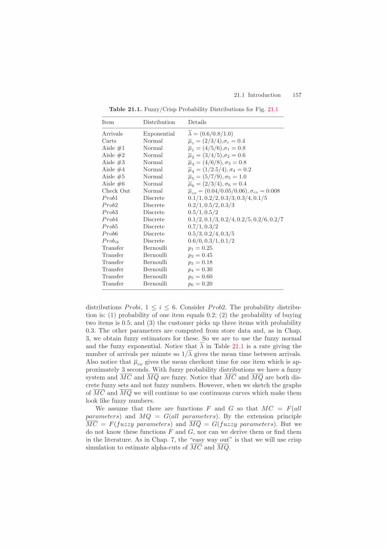
21.1 Introduction 157
Table 21.1. Fuzzy/Crisp Probability Distributions for Fig. 21.1
Item Distribution Details
Arrivals Exponential λ = (0.6/0.8/1.0)Carts Normal µc = (2/3/4),σc = 0.4Aisle #1 Normal µ1 = (4/5/6),σ1 = 0.8Aisle #2 Normal µ2 = (3/4/5),σ2 = 0.6Aisle #3 Normal µ3 = (4/6/8), σ3 = 0.8Aisle #4 Normal µ4 = (1/2.5/4), σ4 = 0.2Aisle #5 Normal µ5 = (5/7/9), σ5 = 1.0Aisle #6 Normal µ6 = (2/3/4), σ6 = 0.4Check Out Normal µco = (0.04/0.05/0.06), σco = 0.008Prob1 Discrete 0.1/1, 0.2/2, 0.3/3, 0.3/4, 0.1/5Prob2 Discrete 0.2/1, 0.5/2, 0.3/3Prob3 Discrete 0.5/1, 0.5/2Prob4 Discrete 0.1/2, 0.1/3, 0.2/4, 0.2/5, 0.2/6, 0.2/7Prob5 Discrete 0.7/1, 0.3/2Prob6 Discrete 0.5/3, 0.2/4, 0.3/5Probib Discrete 0.6/0, 0.3/1, 0.1/2Transfer Bernoulli p1 = 0.25Transfer Bernoulli p2 = 0.45Transfer Bernoulli p3 = 0.18Transfer Bernoulli p4 = 0.30Transfer Bernoulli p5 = 0.60Transfer Bernoulli p6 = 0.20
distributions Probi, 1 ≤ i ≤ 6. Consider Prob2. The probability distribu-tion is: (1) probability of one item equals 0.2; (2) the probability of buyingtwo items is 0.5; and (3) the customer picks up three items with probability0.3. The other parameters are computed from store data and, as in Chap.3, we obtain fuzzy estimators for these. So we are to use the fuzzy normaland the fuzzy exponential. Notice that λ in Table 21.1 is a rate giving thenumber of arrivals per minute so 1/λ gives the mean time between arrivals.Also notice that µco gives the mean checkout time for one item which is ap-proximately 3 seconds. With fuzzy probability distributions we have a fuzzysystem and MC and MQ are fuzzy. Notice that MC and MQ are both dis-crete fuzzy sets and not fuzzy numbers. However, when we sketch the graphsof MC and MQ we will continue to use continuous curves which make themlook like fuzzy numbers.
We assume that there are functions F and G so that MC = F (allparameters) and MQ = G(all parameters). By the extension principleMC = F (fuzzy parameters) and MQ = G(fuzzy parameters). But wedo not know these functions F and G, nor can we derive them or find themin the literature. As in Chap. 7, the “easy way out” is that we will use crispsimulation to estimate alpha-cuts of MC and MQ.
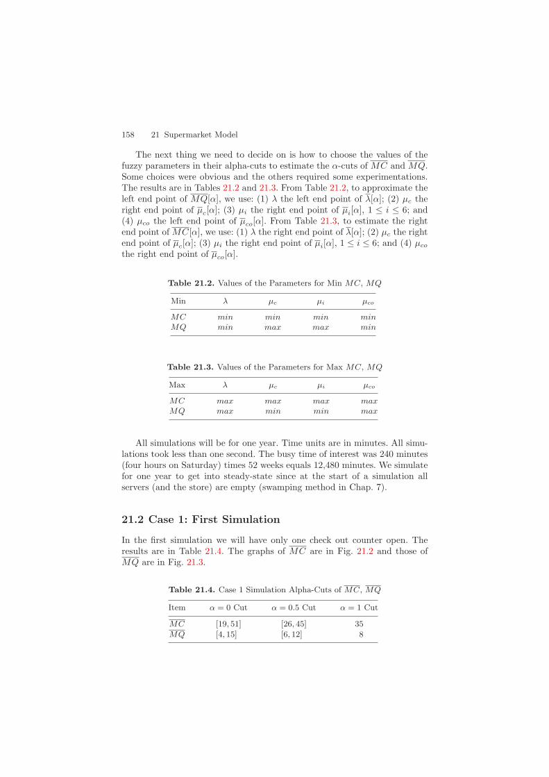
158 21 Supermarket Model
The next thing we need to decide on is how to choose the values of thefuzzy parameters in their alpha-cuts to estimate the α-cuts of MC and MQ.Some choices were obvious and the others required some experimentations.The results are in Tables 21.2 and 21.3. From Table 21.2, to approximate theleft end point of MQ[α], we use: (1) λ the left end point of λ[α]; (2) µc theright end point of µc[α]; (3) µi the right end point of µi[α], 1 ≤ i ≤ 6; and(4) µco the left end point of µco[α]. From Table 21.3, to estimate the rightend point of MC[α], we use: (1) λ the right end point of λ[α]; (2) µc the rightend point of µc[α]; (3) µi the right end point of µi[α], 1 ≤ i ≤ 6; and (4) µco
the right end point of µco[α].
Table 21.2. Values of the Parameters for Min MC, MQ
Min λ µc µi µco
MC min min min minMQ min max max min
Table 21.3. Values of the Parameters for Max MC, MQ
Max λ µc µi µco
MC max max max maxMQ max min min max
All simulations will be for one year. Time units are in minutes. All simu-lations took less than one second. The busy time of interest was 240 minutes(four hours on Saturday) times 52 weeks equals 12,480 minutes. We simulatefor one year to get into steady-state since at the start of a simulation allservers (and the store) are empty (swamping method in Chap. 7).
21.2 Case 1: First Simulation
In the first simulation we will have only one check out counter open. Theresults are in Table 21.4. The graphs of MC are in Fig. 21.2 and those ofMQ are in Fig. 21.3.
Table 21.4. Case 1 Simulation Alpha-Cuts of MC, MQ
Item α = 0 Cut α = 0.5 Cut α = 1 Cut
MC [19, 51] [26, 45] 35
MQ [4, 15] [6, 12] 8
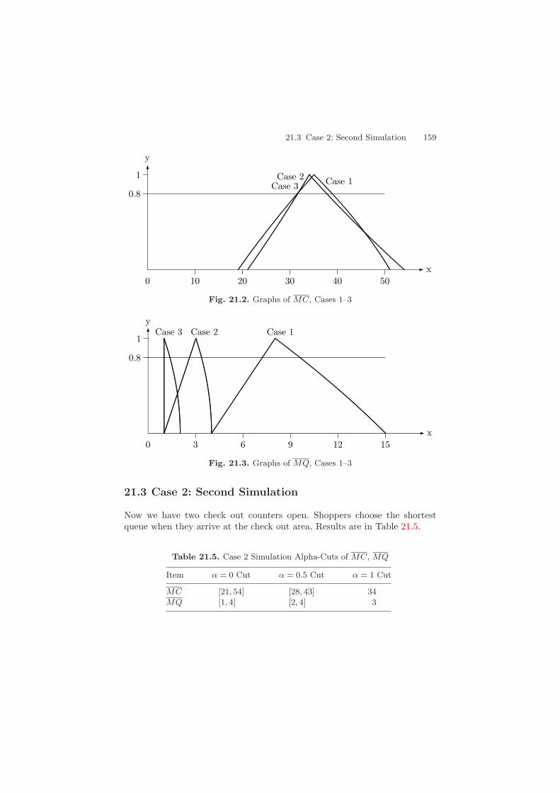
21.3 Case 2: Second Simulation 159
0.8
0 10 20 30 40 50x
1
y
Case 2 Case 1Case 3
Fig. 21.2. Graphs of MC, Cases 1–3
0.8
0 3 6 9 12 15x
1
yCase 2 Case 1Case 3
Fig. 21.3. Graphs of MQ, Cases 1–3
21.3 Case 2: Second Simulation
Now we have two check out counters open. Shoppers choose the shortestqueue when they arrive at the check out area. Results are in Table 21.5.
Table 21.5. Case 2 Simulation Alpha-Cuts of MC, MQ
Item α = 0 Cut α = 0.5 Cut α = 1 Cut
MC [21, 54] [28, 43] 34
MQ [1, 4] [2, 4] 3

160 21 Supermarket Model
21.4 Case 3: Third Simulation
All three check out counters are now open. Simulation alpha-cuts are inTable 21.6.
Table 21.6. Case 3 Simulation Alpha-Cuts of MC, MQ
Item α = 0 Cut α = 0.5 Cut α = 1 Cut
MC [21, 54] [28, 42] 34
MQ [1, 2] [1, 2] 1
21.5 Summary
We see from Fig. 21.2 that the number of open check out counters does notseem to have any effect on the maximum number of shopping carts in use.Figure 21.3 shows that, as would be expected, the maximum queue lengthdecreases as more check out counters are opened. Management decides ontwo open check out lanes because the slight decrease in MQ when we openthe third check out counter doesn’t seem worth the extra expense of the thirdclerk. In this chapter MC and MQ are discrete fuzzy sets whose graphs areapproximated by a continuous fuzzy set (Sect. 2.7).
Reference
1. Thomas J. Schriber: Simulation Using GPSS, John Wiley and Sons, New York,1974. 155
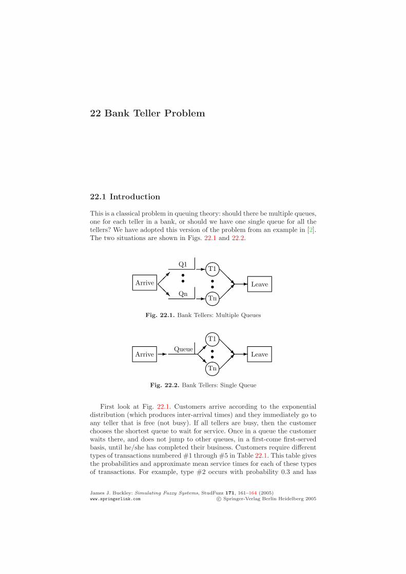
22 Bank Teller Problem
22.1 Introduction
This is a classical problem in queuing theory: should there be multiple queues,one for each teller in a bank, or should we have one single queue for all thetellers? We have adopted this version of the problem from an example in [2].The two situations are shown in Figs. 22.1 and 22.2.
Arrive
Q1
Qn
T1
Tn
Leave
Fig. 22.1. Bank Tellers: Multiple Queues
Arrive Queue
T1
Tn
Leave
Fig. 22.2. Bank Tellers: Single Queue
First look at Fig. 22.1. Customers arrive according to the exponentialdistribution (which produces inter-arrival times) and they immediately go toany teller that is free (not busy). If all tellers are busy, then the customerchooses the shortest queue to wait for service. Once in a queue the customerwaits there, and does not jump to other queues, in a first-come first-servedbasis, until he/she has completed their business. Customers require differenttypes of transactions numbered #1 through #5 in Table 22.1. This table givesthe probabilities and approximate mean service times for each of these typesof transactions. For example, type #2 occurs with probability 0.3 and has
James J. Buckley: Simulating Fuzzy Systems, StudFuzz 171, 161–164 (2005)www.springerlink.com c© Springer-Verlag Berlin Heidelberg 2005
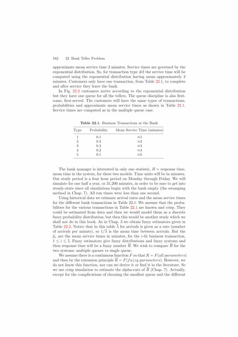
162 22 Bank Teller Problem
approximate mean service time 2 minutes. Service times are governed by theexponential distribution. So, for transaction type #2 the service time will becomputed using the exponential distribution having mean approximately 2minutes. Customers only have one transaction, from Table 22.1, to completeand after service they leave the bank.
In Fig. 22.2 customers arrive according to the exponential distributionbut they have one queue for all the tellers. The queue discipline is also first-come, first-served. The customers still have the same types of transactions,probabilities and approximate mean service times as shown in Table 22.1.Service times are computed as in the multiple queue case.
Table 22.1. Business Transactions at the Bank
Type Probability Mean Service Time (minutes)
1 0.1 ≈12 0.3 ≈23 0.3 ≈34 0.2 ≈45 0.1 ≈5
The bank manager is interested in only one statistic, R = response time,mean time in the system, for these two models. Time units will be in minutes.Our study period is a four hour period on Monday through Friday. We willsimulate for one half a year, or 31,200 minutes, in order to be sure to get intosteady-state since all simulations begin with the bank empty (the swampingmethod in Chap. 7). All run times were less than one second.
Using historical data we estimate arrival rates and the mean service timesfor the different bank transactions in Table 22.1. We assume that the proba-bilities for the various transactions in Table 22.1 are known and crisp. Theycould be estimated from data and then we would model them as a discretefuzzy probability distribution; but then this would be another study which weshall not do in this book. As in Chap. 3 we obtain fuzzy estimators given inTable 22.2. Notice that in this table λ for arrivals is given as a rate (numberof arrivals per minute), so 1/λ is the mean time between arrivals. But theµi are the mean service times in minutes, for the i-th business transaction,1 ≤ i ≤ 5. Fuzzy estimators give fuzzy distributions and fuzzy systems andthen response time will be a fuzzy number R. We wish to compare R for thetwo systems: multiple queues vs single queue.
We assume there is a continuous function F so that R = F (all parameters)and then by the extension principle R = F (fuzzy parameters). However, wedo not know this function, nor can we derive it or find it in the literature. Sowe use crisp simulation to estimate the alpha-cuts of R (Chap. 7). Actually,except for the complications of choosing the smallest queue and the different

22.4 Summary 163
Table 22.2. Fuzzy/Crisp Probability Distributions for the Bank
Item Distribution Details
Arrivals Exponential λa = (0.5/1/1.5) rateService #1 Exponential µ1 = (0.5/1/1.5) timeService #2 Exponential µ2 = (1/2/3) timeService #3 Exponential µ3 = (2/3/4) timeService #4 Exponential µ4 = (3/4/5) timeService #5 Exponential µ5 = (4/5/6) timeTransactions Discrete 0.1/1, 0.3/2, 0.3/3, 0.2/4, 0.1/5
transactions in Table 22.1, an F could be found in most operations researchtext books [1].
The last thing we need to do before simulation is to decide on how tochoose the parameters in their alpha-cuts to estimate the end points of theintervals R[α]. In this problem this is easily solved: (1) for the left end pointof R[α] use λ the left end point of λ[α] and use µi the left end point of µi[α],1 ≤ i ≤ 5; and (2) for the right end point of R[α] use λ the right end pointof λ[α] and use µi the right end point of µi[α], 1 ≤ i ≤ 5.
22.2 First Simulation: Multiple Queues
The simulation results are in Table 22.3 and graphs of R are in Fig. 22.3.For the rest of this chapter we assume that there are six tellers. The bankmanager does not want to hire more tellers.
Table 22.3. Multiple Queues Simulation Alpha-Cuts of R
Item α = 0 Cut α = 0.5 Cut α = 1 Cut
R [1.976, 16.504] [2.475, 4.569] 3.180
22.3 Second Simulation: Single Queue
The simulation results are in Table 22.4 and the graph of R is in Fig. 22.3.
22.4 Summary
We see from Fig. 22.3 that there is not much difference in the time spent inthe system for the two models. The base of these fuzzy numbers is like a 99%

164 22 Bank Teller Problem
0.8
0 4 8 12 16 20x
1
y
Multiple Queues Single Queue
Fig. 22.3. Graphs of R (Minutes)
Table 22.4. Single Queue Simulation Alpha-Cuts of R
Item α = 0 Cut α = 0.5 Cut α = 1 Cut
R [1.976, 21.690] [2.456, 4.105] 3.036
confidence interval. However, multiple queue R has less uncertainty than thesingle queue R. It looks like we almost have multiple queue R a fuzzy subsetof the single queue R (Sect. 2.2.3 of Chap. 2). We would recommend thesingle queue method (see below).
There are situations where one model may do better (less response time)that the other model. In fact, for the multiple queue model, if we let customerschange queues to the faster moving line, then its response time should de-crease and the multiple queue model may be doing a little better than thesingle queue model.
Many banks in the US have changed to the single queue model. Whenasked why the change the answer was usually that it gives the customermore privacy with the teller. This bank manager sees that both models giveapproximately the same response time, the multiple queue method has lessuncertainty but the single queue allows more privacy, so the bank managerchanges to the single queue. A GPSS program for the single queue model isin Chap. 28.
References
1. H.A. Taha: Operations Research, Fifth Edition, Macmillan, New York, 1992. 1632. Thomas J. Schriber: Simulation Using GPSS, John Wiley and Sons, New York,
1974. 161
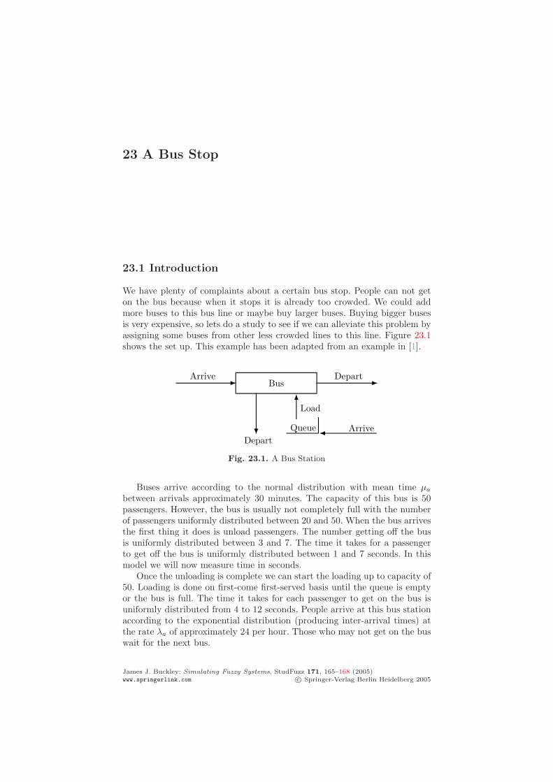
23 A Bus Stop
23.1 Introduction
We have plenty of complaints about a certain bus stop. People can not geton the bus because when it stops it is already too crowded. We could addmore buses to this bus line or maybe buy larger buses. Buying bigger busesis very expensive, so lets do a study to see if we can alleviate this problem byassigning some buses from other less crowded lines to this line. Figure 23.1shows the set up. This example has been adapted from an example in [1].
BusArrive Depart
QueueDepart
Load
Arrive
Fig. 23.1. A Bus Station
Buses arrive according to the normal distribution with mean time µa
between arrivals approximately 30 minutes. The capacity of this bus is 50passengers. However, the bus is usually not completely full with the numberof passengers uniformly distributed between 20 and 50. When the bus arrivesthe first thing it does is unload passengers. The number getting off the busis uniformly distributed between 3 and 7. The time it takes for a passengerto get off the bus is uniformly distributed between 1 and 7 seconds. In thismodel we will now measure time in seconds.
Once the unloading is complete we can start the loading up to capacity of50. Loading is done on first-come first-served basis until the queue is emptyor the bus is full. The time it takes for each passenger to get on the bus isuniformly distributed from 4 to 12 seconds. People arrive at this bus stationaccording to the exponential distribution (producing inter-arrival times) atthe rate λa of approximately 24 per hour. Those who may not get on the buswait for the next bus.
James J. Buckley: Simulating Fuzzy Systems, StudFuzz 171, 165–168 (2005)www.springerlink.com c© Springer-Verlag Berlin Heidelberg 2005
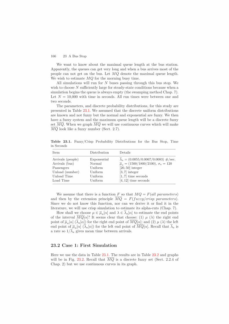
166 23 A Bus Stop
We want to know about the maximal queue length at the bus station.Apparently, the queues can get very long and when a bus arrives most of thepeople can not get on the bus. Let MQ denote the maximal queue length.We wish to estimate MQ for the morning busy time.
All simulations will run for N buses passing through this bus stop. Wewish to choose N sufficiently large for steady-state conditions because when asimulation begins the queue is always empty (the swamping method Chap. 7).Let N = 10,000 with time in seconds. All run times were between one andtwo seconds.
The parameters, and discrete probability distributions, for this study arepresented in Table 23.1. We assumed that the discrete uniform distributionsare known and not fuzzy but the normal and exponential are fuzzy. We thenhave a fuzzy system and the maximum queue length will be a discrete fuzzyset MQ. When we graph MQ we will use continuous curves which will makeMQ look like a fuzzy number (Sect. 2.7).
Table 23.1. Fuzzy/Crisp Probability Distributions for the Bus Stop, Timein Seconds
Item Distribution Details
Arrivals (people) Exponential λa = (0.0055/0.0067/0.0083) #/sec.Arrivals (bus) Normal µa = (1500/1800/2100), σa = 120Passengers Uniform [20, 50] integerUnload (number) Uniform [3, 7] integerUnload Time Uniform [1, 7] time secondsLoad Time Uniform [4, 12] time seconds
We assume that there is a function F so that MQ = F (all parameters)and then by the extension principle MQ = F (fuzzy/crisp parameters).Since we do not know this function, nor can we derive it or find it in theliterature, we will use crisp simulation to estimate its alpha-cuts (Chap. 7).
How shall we choose µ ∈ µa[α] and λ ∈ λa[α] to estimate the end pointsof the interval MQ[α]? It seems clear that choose: (1) µ (λ) the right endpoint of µa[α] (λa[α]) for the right end point of MQ[α]; and (2) µ (λ) the leftend point of µa[α] (λa[α]) for the left end point of MQ[α]. Recall that λa isa rate so 1/λa gives mean time between arrivals.
23.2 Case 1: First Simulation
Here we use the data in Table 23.1. The results are in Table 23.2 and graphswill be in Fig. 23.2. Recall that MQ is a discrete fuzzy set (Sect. 2.2.4 ofChap. 2) but we use continuous curves in its graph.
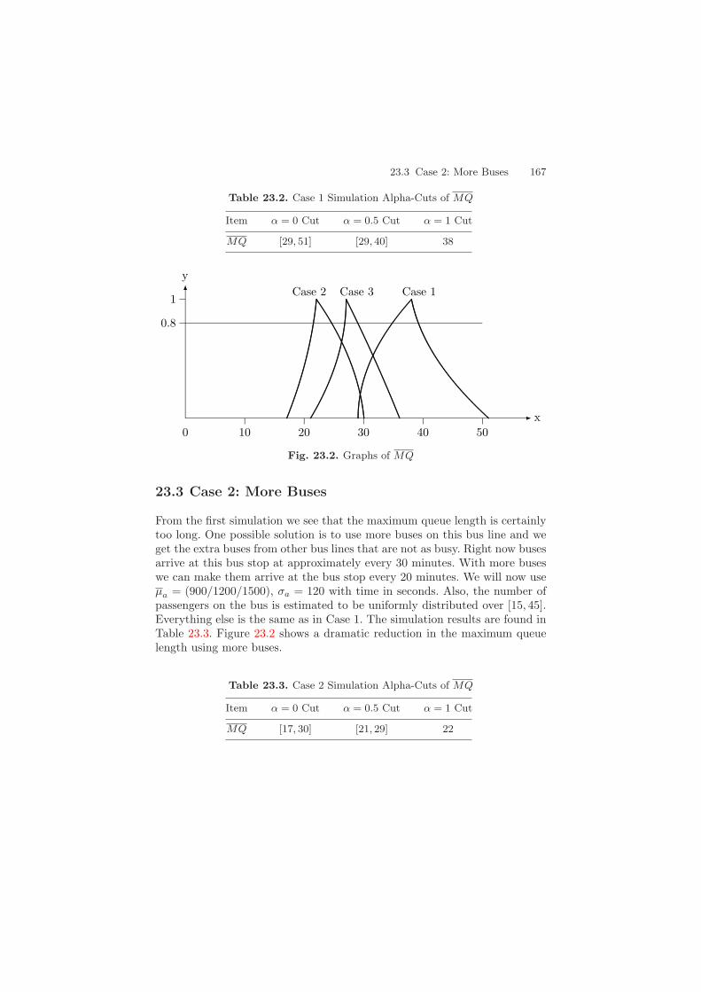
23.3 Case 2: More Buses 167
Table 23.2. Case 1 Simulation Alpha-Cuts of MQ
Item α = 0 Cut α = 0.5 Cut α = 1 Cut
MQ [29, 51] [29, 40] 38
0.8
0 10 20 30 40 50x
1
yCase 1Case 2 Case 3
Fig. 23.2. Graphs of MQ
23.3 Case 2: More Buses
From the first simulation we see that the maximum queue length is certainlytoo long. One possible solution is to use more buses on this bus line and weget the extra buses from other bus lines that are not as busy. Right now busesarrive at this bus stop at approximately every 30 minutes. With more buseswe can make them arrive at the bus stop every 20 minutes. We will now useµa = (900/1200/1500), σa = 120 with time in seconds. Also, the number ofpassengers on the bus is estimated to be uniformly distributed over [15, 45].Everything else is the same as in Case 1. The simulation results are found inTable 23.3. Figure 23.2 shows a dramatic reduction in the maximum queuelength using more buses.
Table 23.3. Case 2 Simulation Alpha-Cuts of MQ
Item α = 0 Cut α = 0.5 Cut α = 1 Cut
MQ [17, 30] [21, 29] 22

168 23 A Bus Stop
23.4 Case 3: Larger Buses
Another possible solution is to purchase larger buses. This method will bevery expensive but the city council still would like to see the results for largerbuses. Assume that the new buses have capacity 80 passengers. These buseswill arrive at this bus stop approximately every 30 minutes, the number ofpeople on the bus is uniformly distributed on [20, 50], etc. In fact all the datais the same as in Table 23.1. So we change the capacity to 80 in the simulationprogram producing the results in Table 23.4.
Table 23.4. Case 3 Simulation Alpha-Cuts of MQ
Item α = 0 Cut α = 0.5 Cut α = 1 Cut
MQ [21, 36] [27, 32] 27
23.5 Summary
Let MQi be the outcome for Case i = 1, 2, 3. Figure 23.2 clearly shows thatMQ2 < MQ3 < MQ1 (see Sect. 2.5 of Chap. 2) and we do not have to buythe bigger buses for now. We just need to transfer some buses from less busyroutes to this bus route to substantially reduce the maximum queue length.
Reference
1. Thomas J. Schriber: Simulation Using GPSS, John Wiley and Sons, New York,1974. 165
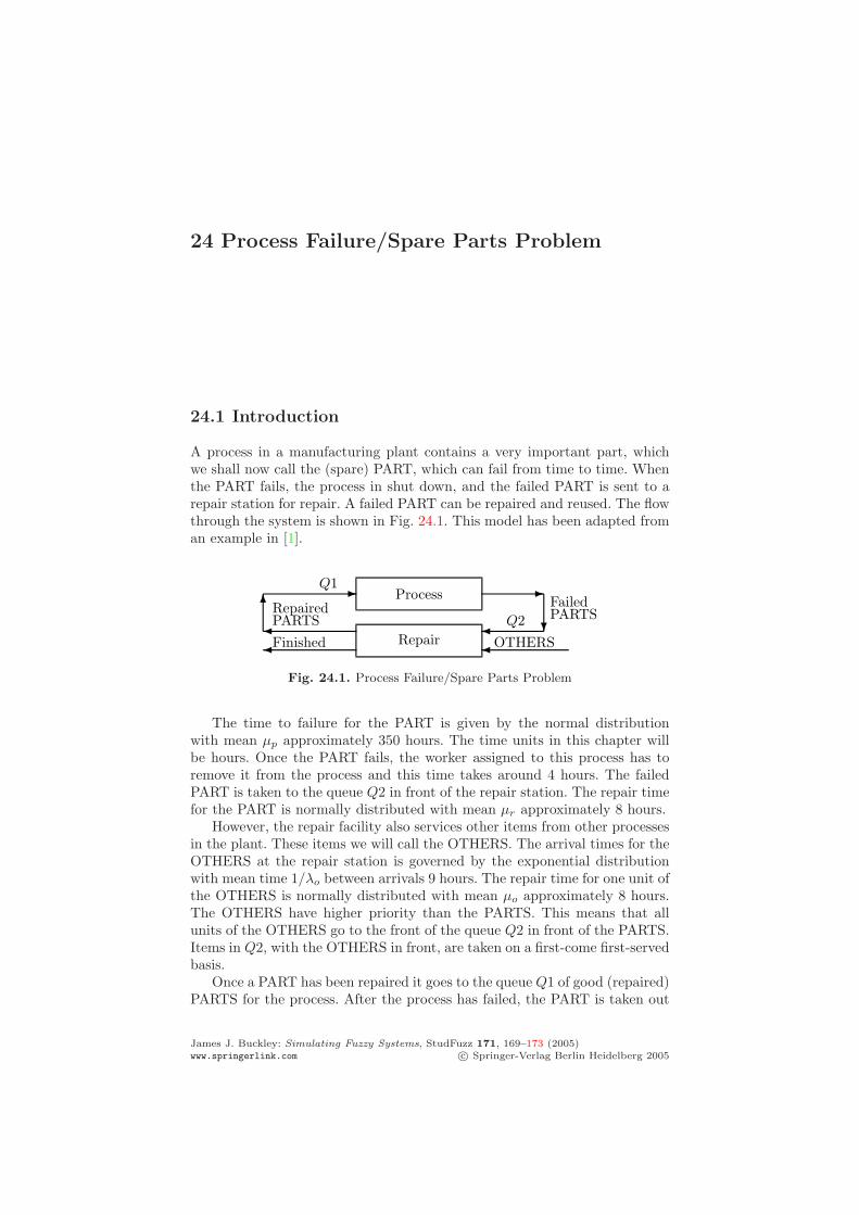
24 Process Failure/Spare Parts Problem
24.1 Introduction
A process in a manufacturing plant contains a very important part, whichwe shall now call the (spare) PART, which can fail from time to time. Whenthe PART fails, the process in shut down, and the failed PART is sent to arepair station for repair. A failed PART can be repaired and reused. The flowthrough the system is shown in Fig. 24.1. This model has been adapted froman example in [1].
ProcessQ1
Repair
Q2
OTHERS
FailedPARTS
Finished
RepairedPARTS
Fig. 24.1. Process Failure/Spare Parts Problem
The time to failure for the PART is given by the normal distributionwith mean µp approximately 350 hours. The time units in this chapter willbe hours. Once the PART fails, the worker assigned to this process has toremove it from the process and this time takes around 4 hours. The failedPART is taken to the queue Q2 in front of the repair station. The repair timefor the PART is normally distributed with mean µr approximately 8 hours.
However, the repair facility also services other items from other processesin the plant. These items we will call the OTHERS. The arrival times for theOTHERS at the repair station is governed by the exponential distributionwith mean time 1/λo between arrivals 9 hours. The repair time for one unit ofthe OTHERS is normally distributed with mean µo approximately 8 hours.The OTHERS have higher priority than the PARTS. This means that allunits of the OTHERS go to the front of the queue Q2 in front of the PARTS.Items in Q2, with the OTHERS in front, are taken on a first-come first-servedbasis.
Once a PART has been repaired it goes to the queue Q1 of good (repaired)PARTS for the process. After the process has failed, the PART is taken out
James J. Buckley: Simulating Fuzzy Systems, StudFuzz 171, 169–173 (2005)www.springerlink.com c© Springer-Verlag Berlin Heidelberg 2005

170 24 Process Failure/Spare Parts Problem
and sent to Q2, and then the worker goes to Q1 to get a good PART. If Q1is empty he must wait for the first repaired PART. If there is a good PARTin Q1 the worker takes it and installs it into the process. Installation time isapproximately 6 hours.
Management wants to determine the utilization U of the process as afunction of the number of PARTS in the system. So, we are to determineutilization U of the process for PARTS = 1, 2, 3, or 4. A spare part is anextra PART. If PARTS = 1, then spare PARTS = 0, and if PARTS = 2, thenspare PARTS = 1, etc. All simulations will be for 10,400 hours which equalsfive years at 40 hours per week. The long simulation runs are to get us intosteady-state since at the start of any simulation the PART is “good” and Q2is empty (the swamping method in Chap. 7).
All the parameters are needed to be estimated from expert opinion(Sects. 3.2, 12.1) or from historical data. Therefore, we use fuzzy estima-tors for all the parameters. These are defined in Table 24.1. Notice that thetwo constants, time to remove (RP) and time to install (IP) a PART, becomefuzzy numbers. Also, as usual, λo is given as the rate of the number of arrivalsper hour. Since the constants are fuzzy numbers and we are using the fuzzynormal and the fuzzy exponential, the system becomes fuzzy and utilizationU will be a fuzzy number.
We assume there is a function F so that U = F (all parameters) andby the extension principle U = F (fuzzy parameters). We do not know thisfunction, nor can we derive it or find it in the literature. Hence, we employsimulation to estimate the end points of the alpha-cuts of U (see Chap. 7).All simulations took less than one second.
The last thing to do before we can use simulation is to decide how to pickthe values of the parameters in their α-cuts to estimate the end points of theintervals U [α]. After some experimentation, the results are in Tables 24.2 and24.3. We found only a small effect on U from varying RP (time to removethe PART) and IP (time to install the PART). We interpret Table 24.2 toestimate the left end point of U [α] as follows: (1) use the left end point ofµp[α]; and (2) use the right end point of λo[α], µr[α], µo[α]. To estimate the
Table 24.1. Fuzzy Probability Distributions for the Process Failure/Spare PartsProblem
Item Distribution Details
Failures Normal µp = (300/350/400), σp = 60
Arrivals (OTHERS) Exponential λo = (0.091/0.111/0.143)Remove PART (RP) Constant RP = (3/4/5)Install PART (IP) Constant IP = (5/6/7)Repair PART Normal µr = (6/8/10),σr = 1.2Repair OTHERS Normal µo = (6/8/10),σo = 1.2
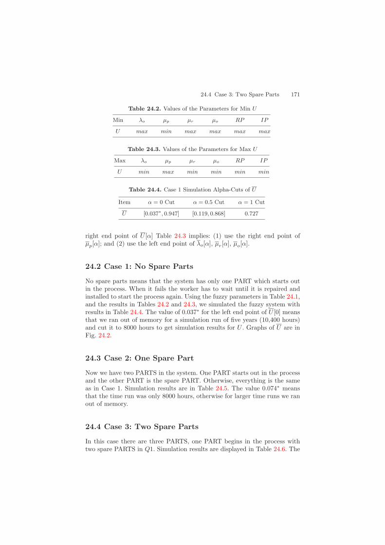
24.4 Case 3: Two Spare Parts 171
Table 24.2. Values of the Parameters for Min U
Min λo µp µr µo RP IP
U max min max max max max
Table 24.3. Values of the Parameters for Max U
Max λo µp µr µo RP IP
U min max min min min min
Table 24.4. Case 1 Simulation Alpha-Cuts of U
Item α = 0 Cut α = 0.5 Cut α = 1 Cut
U [0.037∗, 0.947] [0.119, 0.868] 0.727
right end point of U [α] Table 24.3 implies: (1) use the right end point ofµp[α]; and (2) use the left end point of λo[α], µr[α], µo[α].
24.2 Case 1: No Spare Parts
No spare parts means that the system has only one PART which starts outin the process. When it fails the worker has to wait until it is repaired andinstalled to start the process again. Using the fuzzy parameters in Table 24.1,and the results in Tables 24.2 and 24.3, we simulated the fuzzy system withresults in Table 24.4. The value of 0.037∗ for the left end point of U [0] meansthat we ran out of memory for a simulation run of five years (10,400 hours)and cut it to 8000 hours to get simulation results for U . Graphs of U are inFig. 24.2.
24.3 Case 2: One Spare Part
Now we have two PARTS in the system. One PART starts out in the processand the other PART is the spare PART. Otherwise, everything is the sameas in Case 1. Simulation results are in Table 24.5. The value 0.074∗ meansthat the time run was only 8000 hours, otherwise for larger time runs we ranout of memory.
24.4 Case 3: Two Spare Parts
In this case there are three PARTS, one PART begins in the process withtwo spare PARTS in Q1. Simulation results are displayed in Table 24.6. The
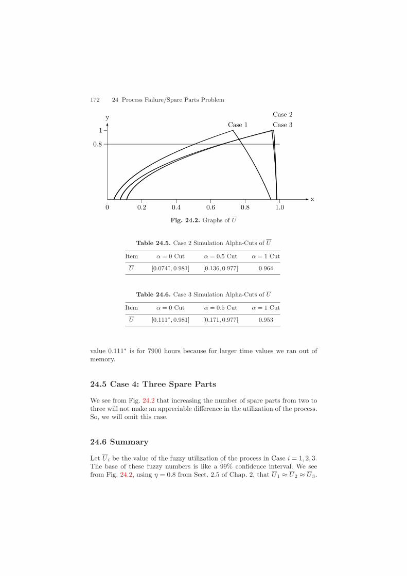
172 24 Process Failure/Spare Parts Problem
0.8
0 0.2 0.4 0.6 0.8 1.0x
1
yCase 1
Case 2Case 3
Fig. 24.2. Graphs of U
Table 24.5. Case 2 Simulation Alpha-Cuts of U
Item α = 0 Cut α = 0.5 Cut α = 1 Cut
U [0.074∗, 0.981] [0.136, 0.977] 0.964
Table 24.6. Case 3 Simulation Alpha-Cuts of U
Item α = 0 Cut α = 0.5 Cut α = 1 Cut
U [0.111∗, 0.981] [0.171, 0.977] 0.953
value 0.111∗ is for 7900 hours because for larger time values we ran out ofmemory.
24.5 Case 4: Three Spare Parts
We see from Fig. 24.2 that increasing the number of spare parts from two tothree will not make an appreciable difference in the utilization of the process.So, we will omit this case.
24.6 Summary
Let U i be the value of the fuzzy utilization of the process in Case i = 1, 2, 3.The base of these fuzzy numbers is like a 99% confidence interval. We seefrom Fig. 24.2, using η = 0.8 from Sect. 2.5 of Chap. 2, that U1 ≈ U2 ≈ U3.
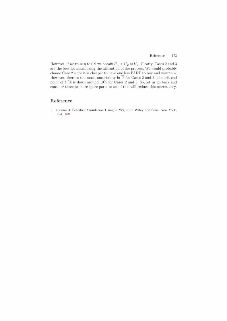
Reference 173
However, if we raise η to 0.9 we obtain U1 < U2 ≈ U3. Clearly, Cases 2 and 3are the best for maximizing the utilization of the process. We would probablychoose Case 2 since it is cheaper to have one less PART to buy and maintain.However, there is too much uncertainty in U for Cases 2 and 3. The left endpoint of U [0] is down around 10% for Cases 2 and 3. So, let us go back andconsider three or more spare parts to see if this will reduce this uncertainty.
Reference
1. Thomas J. Schriber: Simulation Using GPSS, John Wiley and Sons, New York,1974. 169

25 Preemptive Service
25.1 Introduction
A small city has a small municipal garage that does maintenance and repairon city owned vehicles. There are two types of vehicles: (1) TYPE 1 is thecity owned cars, trucks, etc.; and (2) TYPE 2 is all the police cars. TYPE1 vehicles get scheduled, from time to time, for maintenance and repair. AllTYPE 1 vehicles scheduled for maintenance/repair on a certain day arrivebefore the garage opens at 8 am on that day and queue up ready for service.The number of TYPE 1 vehicles scheduled for maintenance/repair on anyday is uniformly distributed between one and ten. That is, there is a randomvariable X with values 1, 2, . . . , 10 each with probability 0.1 and the value ofX is the number of vehicles ready for service on any day. The city garage issmall with one service bay and only one mechanic at work. Service can beperformed on only one vehicle at a time. The garage is open from 8 am to4 pm seven days per week. The 8 hours per day seven day per week requireshiring more than one mechanic, but only one mechanic is working at any time.The service time for TYPE 1 vehicles is normally distributed with mean µ1
approximately 2 hours. Any TYPE 1 vehicle not serviced on its scheduledday waits for service on the following day. The time units in this chapter willbe minutes so µ1 ≈ 120.
TYPE 2 vehicles (police cars) can randomly experience a problem requir-ing maintence/repair any time in a 24 hour day. When this happens theyhave an unscheduled maintenance/repair time at the city garage. Police carsmay arrive any time of the day, or night, at the garage for service. Of course,if they arrive when it is closed the car must wait until 8 am when it opens.TYPE 2 vehicles have preemptive service. What this means is: (1) if the ser-vice bay is vacant they immediately go in for service; (1) if a TYPE 1 vehicleis now being serviced it is removed from the service bay and the police carenters the service bay for service; and (3) if a TYPE 2 vehicle is now beingserviced it must wait until it is finished before it can be serviced. TYPE 2vehicles queue up for service if a TYPE 2 is now being serviced. If a TYPE1 was removed from service for a TYPE 2, time to complete service tc iscomputed, and when it returns to the service bay its service time will betc. Police cars arrive at the garage with inter-arrival time given by the ex-ponential distribution with mean time 1/λ2 between arrivals 24 hours (1440
James J. Buckley: Simulating Fuzzy Systems, StudFuzz 171, 175–179 (2005)www.springerlink.com c© Springer-Verlag Berlin Heidelberg 2005

176 25 Preemptive Service
minutes). As usual, λ2 is the rate of arrivals. Service time for TYPE 2 vehi-cles is normally distributed with mean µ2 approximately 3 hours. A simplefigure for this system is in Fig. 25.1. This problem has been adapted from anexample in [1].
Arrivals
Service
City Vehicles
Police CarsPreemptive
Finished
Fig. 25.1. Preemptive Service Model
The city is interested in keeping the queue lengths for both types of ve-hicles to a minimum. They can not have all their police cars sitting at thegarage waiting for emergency maintenance/repair. Nor can they have thishappen to their TYPE 1 vehicles. Let MQi be the maximum queue lengthfor TYPE i vehicles, i = 1, 2. So, we want to find MQi for the present set up(described above) and consider changes (if needed) to reduce MQ1 and/orMQ2. There are various options to consider, but building a larger city garageis not an option.
All simulations will be for 45 days, or 64800 minutes (24 hours per day).The simulation starts at 8 am, runs for 8 hours while the shop is open, thencloses for 18, to open again at 8 am the next day. Do this for 45 days. Whenthe shop is closed vehicles arrive for service. A sufficiently long simulationrun will get us into steady-state since when we start the queues will be empty(swamping method Chap. 7). All simulation runs took less than one second.
The following probabilities/parameters need to be estimated: (1) the prob-ability of i TYPE 1 vehicles arriving for service, i = 1, 2, . . . , n; (2) µ1 and σ1;(3) λ2; and (4) µ2, σ2. We will assume that the discrete probability distribu-tion for the arrivals of TYPE 1 vehicles is known and crisp. But we estimatethe other parameters from historical data and obtain fuzzy estimators shownin Table 25.1. Recall that λ2 gives the number of police cars arriving at thegarage per minute so 1/λ2 is the mean time in minutes between arrivals. Wenow have the fuzzy normal and the fuzzy exponential implying the system is
Table 25.1. Fuzzy/Crisp Probability Distributions for the Preemptive ServiceProblem, Time in Minutes
Item Distribution Details
Arrivals (TYPE 1) Uniform [1, 10] integerService (TYPE 1) Normal µ1 = (100/120/140), σ1 = 20
Arrivals (TYPE 2) Exponential λ2 = ((1680)−1/(1440)−1/(1200)−1)Service (TYPE 2) Normal µ2 = (120/180/240),σ2 = 24
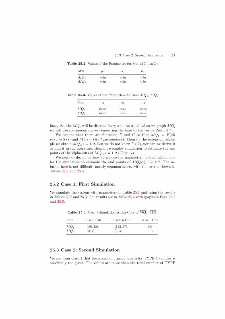
25.3 Case 2: Second Simulation 177
Table 25.2. Values of the Parameters for Min MQ1, MQ2
Min µ1 λ2 µ2
MQ1 min min minMQ2 min min min
Table 25.3. Values of the Parameters for Max MQ1, MQ2
Max µ1 λ2 µ2
MQ1 max max maxMQ2 max max max
fuzzy. So, the MQi will be discrete fuzzy sets. As usual, when we graph MQi
we will use continuous curves connecting the base to the vertex (Sect. 2.7).We assume that there are functions F and G so that MQ1 = F (all
parameters) and MQ2 = G(all parameters). Then by the extension princi-ple we obtain MQi, i = 1, 2. But we do not know F (G), nor can we derive itor find it in the literature. Hence, we employ simulation to estimate the endpoints of the alpha-cuts of MQi, i = 1, 2 (Chap. 7).
We need to decide on how to choose the parameters in their alpha-cutsfor the simulation to estimate the end points of MQi[α], i = 1, 2. The so-lution here is not difficult, mostly common sense, with the results shown inTables 25.2 and 25.3.
25.2 Case 1: First Simulation
We simulate the system with parameters in Table 25.1 and using the resultsin Tables 25.2 and 25.3. The results are in Table 25.4 with graphs in Figs. 25.2and 25.3.
Table 25.4. Case 1 Simulation Alpha-Cuts of MQ1, MQ2
Item α = 0 Cut α = 0.5 Cut α = 1 Cut
MQ1 [86, 228] [112, 171] 141
MQ2 [3, 4] [3, 3] 3
25.3 Case 2: Second Simulation
We see from Case 1 that the maximum queue length for TYPE 1 vehicles isabsolutely too great. The values are more than the total number of TYPE
178 25 Preemptive Service
0.8
0 40 80 120 160 200x
1
yCase 1
Case 2Case 3
Fig. 25.2. Graphs of MQ1
0.8
0 1 2 3 4 5x
1
yCase 2
Case 1Case 3
Fig. 25.3. Graphs of MQ2
1 vehicles owned by the city. Something must be done to reduce MQ1. Thecity decides that much of the service for its TYPE 1 vehicles can be done atlocal gas stations. For example, changing the oil, rotating the types, etc. canbe easily and cheaply accomplished at a gas station. Hence, in the future allof this minor maintenance/repair work will be done at a local gas station.Using this information we estimate the new discrete probability distributionfor the TYPE 1 vehicles arriving at the city garage each day. It is the uni-form distribution on [1, 4]. That is, there is a random variable X with values1, 2, 3, 4, with each value having probability 0.25, giving the number of TYPE1 vehicles each day. This is the only change from Case 1. Simulation resultsare in Table 25.5.
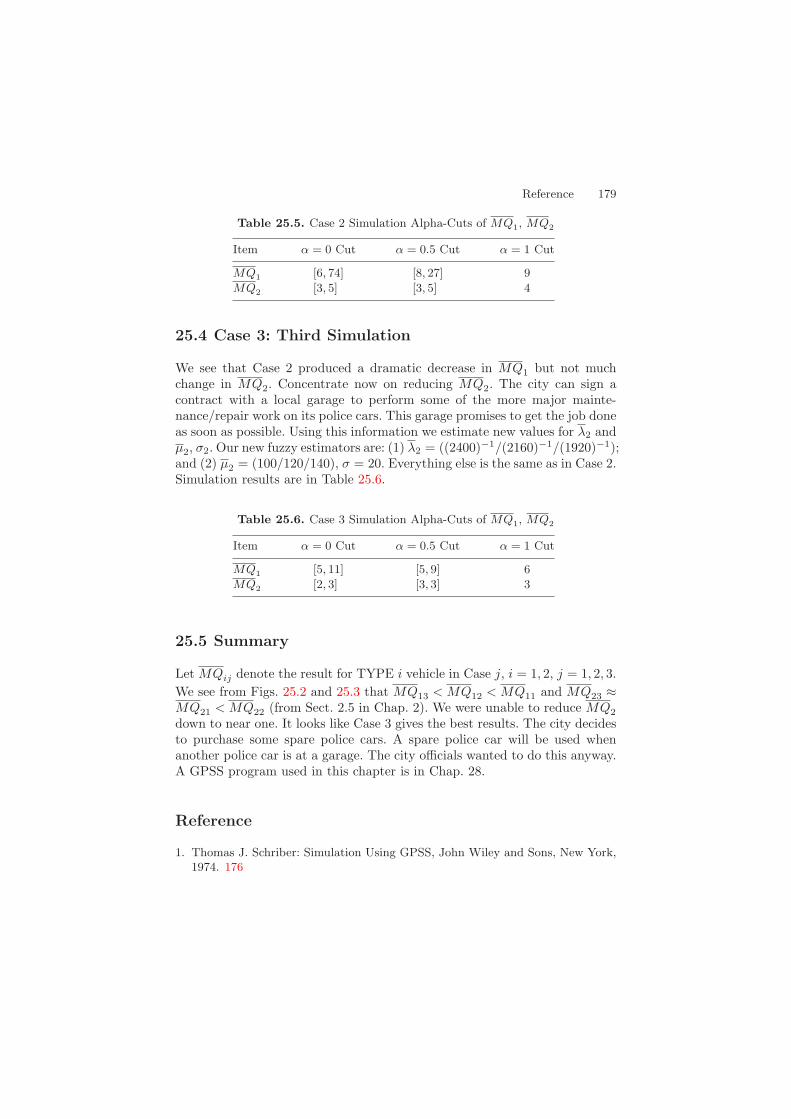
Reference 179
Table 25.5. Case 2 Simulation Alpha-Cuts of MQ1, MQ2
Item α = 0 Cut α = 0.5 Cut α = 1 Cut
MQ1 [6, 74] [8, 27] 9
MQ2 [3, 5] [3, 5] 4
25.4 Case 3: Third Simulation
We see that Case 2 produced a dramatic decrease in MQ1 but not muchchange in MQ2. Concentrate now on reducing MQ2. The city can sign acontract with a local garage to perform some of the more major mainte-nance/repair work on its police cars. This garage promises to get the job doneas soon as possible. Using this information we estimate new values for λ2 andµ2, σ2. Our new fuzzy estimators are: (1) λ2 = ((2400)−1/(2160)−1/(1920)−1);and (2) µ2 = (100/120/140), σ = 20. Everything else is the same as in Case 2.Simulation results are in Table 25.6.
Table 25.6. Case 3 Simulation Alpha-Cuts of MQ1, MQ2
Item α = 0 Cut α = 0.5 Cut α = 1 Cut
MQ1 [5, 11] [5, 9] 6
MQ2 [2, 3] [3, 3] 3
25.5 Summary
Let MQij denote the result for TYPE i vehicle in Case j, i = 1, 2, j = 1, 2, 3.We see from Figs. 25.2 and 25.3 that MQ13 < MQ12 < MQ11 and MQ23 ≈MQ21 < MQ22 (from Sect. 2.5 in Chap. 2). We were unable to reduce MQ2
down to near one. It looks like Case 3 gives the best results. The city decidesto purchase some spare police cars. A spare police car will be used whenanother police car is at a garage. The city officials wanted to do this anyway.A GPSS program used in this chapter is in Chap. 28.
Reference
1. Thomas J. Schriber: Simulation Using GPSS, John Wiley and Sons, New York,1974. 176
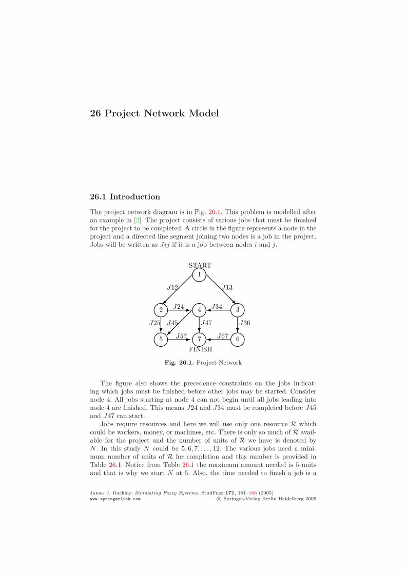
26 Project Network Model
26.1 Introduction
The project network diagram is in Fig. 26.1. This problem is modelled afteran example in [2]. The project consists of various jobs that must be finishedfor the project to be completed. A circle in the figure represents a node in theproject and a directed line segment joining two nodes is a job in the project.Jobs will be written as Jij if it is a job between nodes i and j.
1
START
J12
J13
J24 J34 32
4
J45
J36
J25
J47
5
7
FINISH
6 J67J57
Fig. 26.1. Project Network
The figure also shows the precedence constraints on the jobs indicat-ing which jobs must be finished before other jobs may be started. Considernode 4. All jobs starting at node 4 can not begin until all jobs leading intonode 4 are finished. This means J24 and J34 must be completed before J45and J47 can start.
Jobs require resources and here we will use only one resource R whichcould be workers, money, or machines, etc. There is only so much of R avail-able for the project and the number of units of R we have is denoted byN . In this study N could be 5, 6, 7, . . . , 12. The various jobs need a mini-mum number of units of R for completion and this number is provided inTable 26.1. Notice from Table 26.1 the maximum amount needed is 5 unitsand that is why we start N at 5. Also, the time needed to finish a job is a
James J. Buckley: Simulating Fuzzy Systems, StudFuzz 171, 181–186 (2005)www.springerlink.com c© Springer-Verlag Berlin Heidelberg 2005
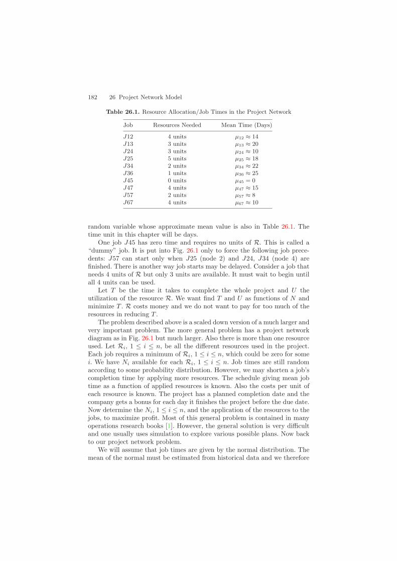
182 26 Project Network Model
Table 26.1. Resource Allocation/Job Times in the Project Network
Job Resources Needed Mean Time (Days)
J12 4 units µ12 ≈ 14J13 3 units µ13 ≈ 20J24 3 units µ24 ≈ 10J25 5 units µ25 ≈ 18J34 2 units µ34 ≈ 22J36 1 units µ36 ≈ 25J45 0 units µ45 = 0J47 4 units µ47 ≈ 15J57 2 units µ57 ≈ 8J67 4 units µ67 ≈ 10
random variable whose approximate mean value is also in Table 26.1. Thetime unit in this chapter will be days.
One job J45 has zero time and requires no units of R. This is called a“dummy” job. It is put into Fig. 26.1 only to force the following job prece-dents: J57 can start only when J25 (node 2) and J24, J34 (node 4) arefinished. There is another way job starts may be delayed. Consider a job thatneeds 4 units of R but only 3 units are available. It must wait to begin untilall 4 units can be used.
Let T be the time it takes to complete the whole project and U theutilization of the resource R. We want find T and U as functions of N andminimize T . R costs money and we do not want to pay for too much of theresources in reducing T .
The problem described above is a scaled down version of a much larger andvery important problem. The more general problem has a project networkdiagram as in Fig. 26.1 but much larger. Also there is more than one resourceused. Let Ri, 1 ≤ i ≤ n, be all the different resources used in the project.Each job requires a minimum of Ri, 1 ≤ i ≤ n, which could be zero for somei. We have Ni available for each Ri, 1 ≤ i ≤ n. Job times are still randomaccording to some probability distribution. However, we may shorten a job’scompletion time by applying more resources. The schedule giving mean jobtime as a function of applied resources is known. Also the costs per unit ofeach resource is known. The project has a planned completion date and thecompany gets a bonus for each day it finishes the project before the due date.Now determine the Ni, 1 ≤ i ≤ n, and the application of the resources to thejobs, to maximize profit. Most of this general problem is contained in manyoperations research books [1]. However, the general solution is very difficultand one usually uses simulation to explore various possible plans. Now backto our project network problem.
We will assume that job times are given by the normal distribution. Themean of the normal must be estimated from historical data and we therefore
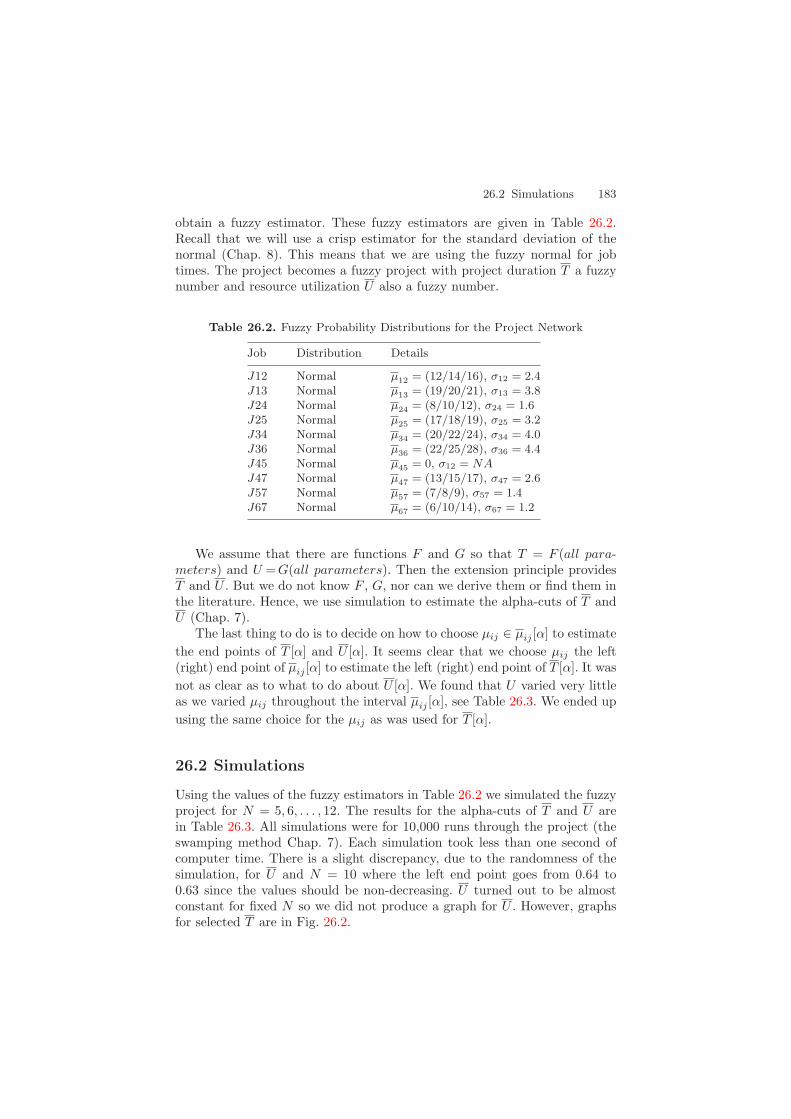
26.2 Simulations 183
obtain a fuzzy estimator. These fuzzy estimators are given in Table 26.2.Recall that we will use a crisp estimator for the standard deviation of thenormal (Chap. 8). This means that we are using the fuzzy normal for jobtimes. The project becomes a fuzzy project with project duration T a fuzzynumber and resource utilization U also a fuzzy number.
Table 26.2. Fuzzy Probability Distributions for the Project Network
Job Distribution Details
J12 Normal µ12 = (12/14/16), σ12 = 2.4J13 Normal µ13 = (19/20/21), σ13 = 3.8J24 Normal µ24 = (8/10/12), σ24 = 1.6J25 Normal µ25 = (17/18/19), σ25 = 3.2J34 Normal µ34 = (20/22/24), σ34 = 4.0J36 Normal µ36 = (22/25/28), σ36 = 4.4J45 Normal µ45 = 0, σ12 = NAJ47 Normal µ47 = (13/15/17), σ47 = 2.6J57 Normal µ57 = (7/8/9), σ57 = 1.4J67 Normal µ67 = (6/10/14), σ67 = 1.2
We assume that there are functions F and G so that T = F (all para-meters) and U = G(all parameters). Then the extension principle providesT and U . But we do not know F , G, nor can we derive them or find them inthe literature. Hence, we use simulation to estimate the alpha-cuts of T andU (Chap. 7).
The last thing to do is to decide on how to choose µij ∈ µij [α] to estimatethe end points of T [α] and U [α]. It seems clear that we choose µij the left(right) end point of µij [α] to estimate the left (right) end point of T [α]. It wasnot as clear as to what to do about U [α]. We found that U varied very littleas we varied µij throughout the interval µij [α], see Table 26.3. We ended upusing the same choice for the µij as was used for T [α].
26.2 Simulations
Using the values of the fuzzy estimators in Table 26.2 we simulated the fuzzyproject for N = 5, 6, . . . , 12. The results for the alpha-cuts of T and U arein Table 26.3. All simulations were for 10,000 runs through the project (theswamping method Chap. 7). Each simulation took less than one second ofcomputer time. There is a slight discrepancy, due to the randomness of thesimulation, for U and N = 10 where the left end point goes from 0.64 to0.63 since the values should be non-decreasing. U turned out to be almostconstant for fixed N so we did not produce a graph for U . However, graphsfor selected T are in Fig. 26.2.
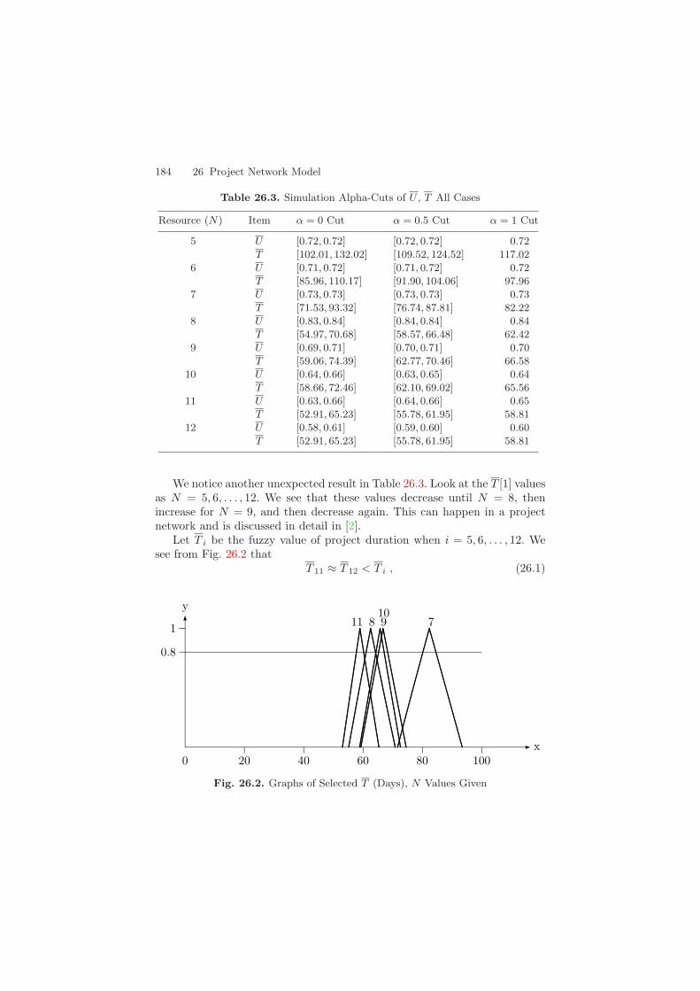
184 26 Project Network Model
Table 26.3. Simulation Alpha-Cuts of U , T All Cases
Resource (N) Item α = 0 Cut α = 0.5 Cut α = 1 Cut
5 U [0.72, 0.72] [0.72, 0.72] 0.72
T [102.01, 132.02] [109.52, 124.52] 117.02
6 U [0.71, 0.72] [0.71, 0.72] 0.72
T [85.96, 110.17] [91.90, 104.06] 97.96
7 U [0.73, 0.73] [0.73, 0.73] 0.73
T [71.53, 93.32] [76.74, 87.81] 82.22
8 U [0.83, 0.84] [0.84, 0.84] 0.84
T [54.97, 70.68] [58.57, 66.48] 62.42
9 U [0.69, 0.71] [0.70, 0.71] 0.70
T [59.06, 74.39] [62.77, 70.46] 66.58
10 U [0.64, 0.66] [0.63, 0.65] 0.64
T [58.66, 72.46] [62.10, 69.02] 65.56
11 U [0.63, 0.66] [0.64, 0.66] 0.65
T [52.91, 65.23] [55.78, 61.95] 58.81
12 U [0.58, 0.61] [0.59, 0.60] 0.60
T [52.91, 65.23] [55.78, 61.95] 58.81
We notice another unexpected result in Table 26.3. Look at the T [1] valuesas N = 5, 6, . . . , 12. We see that these values decrease until N = 8, thenincrease for N = 9, and then decrease again. This can happen in a projectnetwork and is discussed in detail in [2].
Let T i be the fuzzy value of project duration when i = 5, 6, . . . , 12. Wesee from Fig. 26.2 that
T 11 ≈ T 12 < T i , (26.1)
0.8
0 20 40 60 80 100x
1
y8 79
1011
Fig. 26.2. Graphs of Selected T (Days), N Values Given
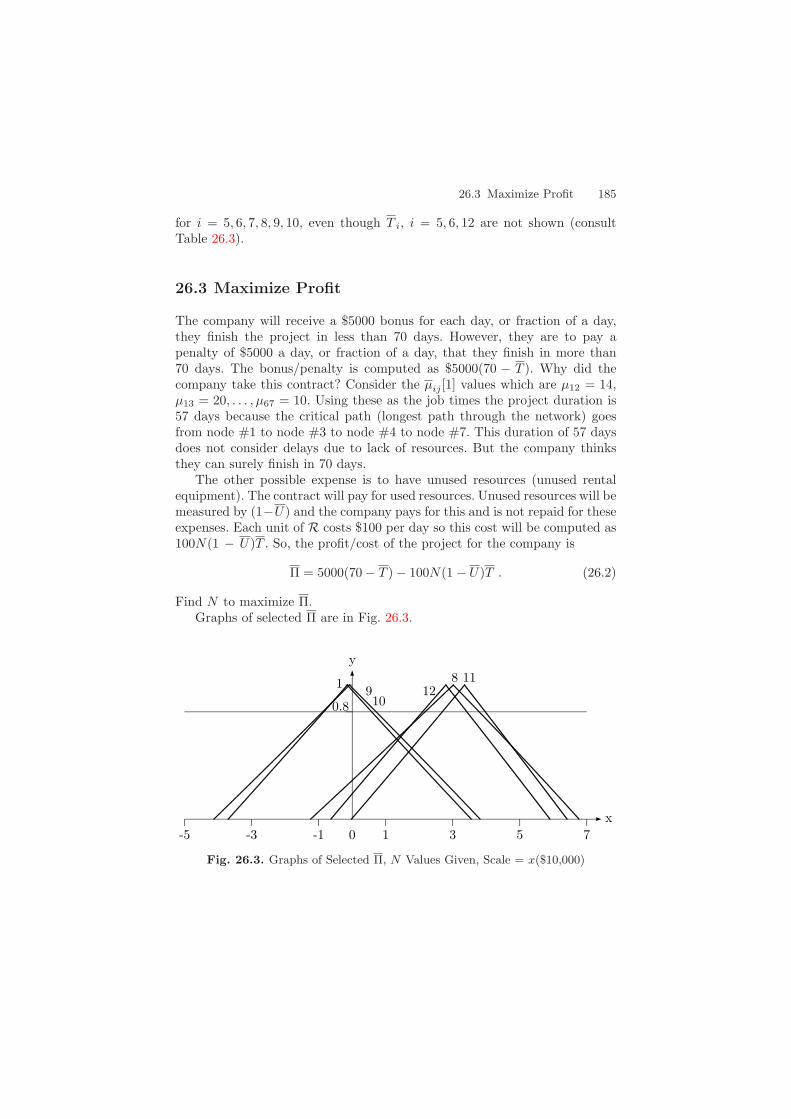
26.3 Maximize Profit 185
for i = 5, 6, 7, 8, 9, 10, even though T i, i = 5, 6, 12 are not shown (consultTable 26.3).
26.3 Maximize Profit
The company will receive a $5000 bonus for each day, or fraction of a day,they finish the project in less than 70 days. However, they are to pay apenalty of $5000 a day, or fraction of a day, that they finish in more than70 days. The bonus/penalty is computed as $5000(70 − T ). Why did thecompany take this contract? Consider the µij [1] values which are µ12 = 14,µ13 = 20, . . . , µ67 = 10. Using these as the job times the project duration is57 days because the critical path (longest path through the network) goesfrom node #1 to node #3 to node #4 to node #7. This duration of 57 daysdoes not consider delays due to lack of resources. But the company thinksthey can surely finish in 70 days.
The other possible expense is to have unused resources (unused rentalequipment). The contract will pay for used resources. Unused resources will bemeasured by (1−U) and the company pays for this and is not repaid for theseexpenses. Each unit of R costs $100 per day so this cost will be computed as100N(1 − U)T . So, the profit/cost of the project for the company is
Π = 5000(70 − T ) − 100N(1 − U)T . (26.2)
Find N to maximize Π.Graphs of selected Π are in Fig. 26.3.
0.8
0-5 -3 -1 1 3 5 7x
1
y8
12910
11
Fig. 26.3. Graphs of Selected Π, N Values Given, Scale = x($10,000)
186 26 Project Network Model
26.4 Summary
Let Πi be the fuzzy profit when i = 5, 6, . . . , 12. We see from Fig. 26.3 (pleasereview Sect. 2.5 of Chap. 2) that
Π9 ≈ Π10 < Π8 ≈ Π11 ≈ Π12 . (26.3)
The base of each Πi is like a 99% confidence interval for profit. What shallwe recommend? We recommend N = 11 because Π11[0] is essentially non-negative. A GPSS program used in this chapter is in Chap. 28.
References
1. H.A. Taha: Operations Research, Fifth Edition, Macmillan, New York, 1992. 1822. Thomas J. Schriber: Simulation Using GPSS, John Wiley and Sons, New York,
1974. 181, 184
27 Summary and Conclusions
The first objective of this book is to explain how many systems naturallybecome fuzzy systems. The second objective is to show how regular (crisp)simulation can be used to estimate the alpha-cuts of the fuzzy numbers usedto analyze the behavior of the fuzzy system.
Consider any system that uses probability distributions in its description.Quite often probabilities and/or parameters in the probability distributions(like the mean of the normal) have to estimated from data or expert opinion.Usually one obtains point estimates of these unknown probabilities and/orparameters for input to the system. However, it would be better to use confi-dence intervals. But which confidence interval should we use? We suggest inChap. 3 to use an infinite set of confidence intervals, stacked up one on topof another, producing fuzzy number estimators. Fuzzy estimators producefuzzy probability distributions in Chap. 4. Now the system is described byfuzzy probabilities and fuzzy probability distributions. It is a fuzzy system(Chap. 5). Things we want to compute, like response time, throughput, etc.all become fuzzy. We need to be able to compute these fuzzy sets and fuzzynumbers.
For some fuzzy systems the computation of the fuzzy descriptors becomesdifficult [1, 2]. We need a faster way to approximate these fuzzy numbers thanmultiple calculations using the extension principle. There is a method usinga readily available technique called simulation. We argue in Chap. 7 that ifthere is a one-step function, and there usually is, that can produce the crispform of the system descriptor, then simulation can be used to approximate thealpha-cuts of the extension principle extension of this function. Simulationmay also be used to approximate some multi-step fuzzy calculations.
But to be able to use simulation to approximate the α-cuts of these fuzzysystem descriptors there are certain optimization problems to solve. Thisis discussed in Chap. 8 and continues in Chaps. 9–26. Consider a simpleexample here where time between arrivals at the system is given by N(µ, σ),the normal distribution, and service times in the system is given by theexponential with mean λ. We want to find X = throughput, or the numberof transactions going through the system in an eight hour day. We estimateµ, σ and λ from data and get fuzzy estimators µ and λ but we use a crisppoint estimator for σ (see Chap. 8). Now find (estimate) the alpha-cuts of
James J. Buckley: Simulating Fuzzy Systems, StudFuzz 171, 187–188 (2005)www.springerlink.com c© Springer-Verlag Berlin Heidelberg 2005
188 27 Summary and Conclusions
fuzzy X. How shall we pick µ ∈ µ[α], λ ∈ λ[α] to have simulation estimatethe left (right) end point of X[α]? This type problem must be solved againand again in Chaps. 9–26. We are to simulate the system with specific valuesof µ, λ and σ to estimate the end points of alpha-cuts of the fuzzy descriptors.
We show how to use simulation to estimate the fuzzy sets/numbers neededto describe the fuzzy system in a great variety of applications in Chaps. 9–26. The applications encompass production lines, emergence rooms, inventorycontrol and project networks.
The one part of this study that is unfinished is theoretical results forsolving the simulation optimization problem (Chap. 8) discussed above. The-oretical results are needed to tell us how to choose the parameters in theiralpha-cuts so that the simulation will estimate the end points of the α-cutsof the fuzzy numbers we need to analyze the fuzzy system. Sometimes weexperimented with different combinations of parameter values to solve thisproblem. We think our results are correct but we have no theoretical justi-fication. Eventually it would be nice to have a “look up” table to find thevalues of these parameters in simulations to estimate the alpha-cuts of thefuzzy numbers. That would make simulation very useful in studying fuzzysystems.
References
1. J.J. Buckley: Fuzzy Probabilities and Fuzzy Sets for Web Planning, Springer,Heidelberg, Germany, 2004. 187
2. J.J. Buckley, K. Reilly and X. Zheng: Fuzzy Probabilities for Web Planning,Soft Computing, 8(2004)464-476. 187

28 Simulation Programs
28.1 Introduction
In this chapter we present some of the GPSS programs used in Chaps. 9–26.We had to omit many programs in order to keep this chapter. less that 20pages long. The reader may obtain other GPSS programs from the author byrequesting them via email.
Most chapters run more than one GPSS simulation but here we give onlyone of these programs. The author does not claim that these programs arethe most efficient. An expert GPSS programmer could certainly make someimprovements to make it run faster. Almost all simulations ran in less than5 seconds so such improvements are not really needed.
We do not give a tutorial on GPSS. References for GPSS were given inChap. 6. It is not the purpose of this book to teach the reader to writeprograms in GPSS. These programs are presented only to show how we didthe simulations. Minimal comments are given for each program written as(comment)
28.2 Chapter 9
1. SIMULATE2. REAL &C(1),&D(1),&M(4),&V(4)3. LET &M(1)=0.125 (Mean of Normal)4. LET &M(2)=0.1255. LET &M(3)=0.0756. LET &M(4)=0.1757. LET &V(1)=0.02 (Standard Deviation of Normal)8. LET &V(2)=0.029. LET &V(3)=0.01
10. LET &V(4)=0.0311. OUT FILEDEF ’ANS1.OUT’ (File for &C(1) and &D(1))12. STORAGE S(SHOP2),213. STORAGE S(SHOP4),314. STORAGE S(INSP),2
James J. Buckley: Simulating Fuzzy Systems, StudFuzz 171, 189–204 (2005)www.springerlink.com c© Springer-Verlag Berlin Heidelberg 2005

190 28 Simulation Programs
15. GENERATE RVEXPO(1,0.1818) (Arrivals)16. QUEUE QUE117. QUEUE QUE218. SEIZE SHOP119. DEPART QUE220. ADVANCE 0.17,0.03 (Time in S1)21. RELEASE SHOP122. TEST E S(SHOP2),0,OUT123. BLET &C(1)=&C(1)+1 (Counts when S2 is Idle)24. OUT1 QUEUE QUE325. ENTER SHOP226. DEPART QUE327. ADVANCE RVNORM(1,&M(1),&V(1)) (Time in S2)28. LEAVE SHOP229. QUEUE QUE430. SEIZE SHOP331. DEPART QUE432. ADVANCE 0.17,0.03 (Time in S3)33. RELEASE SHOP334. TEST E S(SHOP4),0,OUT235. BLET &D(1)=&D(1)+1 (Counts when S4 is Idle)36. OUT2 QUEUE QUE537. ENTER SHOP438. DEPART QUE539. ADVANCE RVNORM(1,&M(2),&V(2)) (Time in S4)40. LEAVE SHOP441. QUEUE QUE6 (Enter the Inspection)42. ENTER INSP43. TEST E F(INSP1),0,OUT3 (Is Inspector #1 Free?)44. SEIZE INSP145. ADVANCE RVNORM(1,&M(3),&V(3)) (Time with Inspector #1)46. RELEASE INSP147. TRANSFER ,OUT448. OUT3 SEIZE INSP2 (Or go to Inspector #2)49. ADVANCE RVNORM(1,&M(4),&V(4)) (Time with Inspector #2)50. RELEASE INSP251. OUT4 LEAVE INSP52. DEPART QUE653. DEPART QUE154. TRANSFER .035,,REJ (Reject with Probability p)55. TERMINATE 156. REJ TERMINATE57. START 10000

28.3 Chapter 10 191
58. PUTPIC FILE=OUT,LINES=3,(&C(1),&D(1))SHOP2=EMPTY ****SHOP4=EMPTY ****
59. END
28.3 Chapter 10
1. SIMULATE2. REAL &L(3),&M(3),&V(3),&C(1),&B(3)3. LET &L(1)=0.2222 (Inter-arrival Times Calls A)4. LET &L(2)=0.2857 (Calls B)5. LET &L(3)=0.4 (Calls C)6. LET &M(1)=0.7 (Mean of Normal for Service X)7. LET &M(2)=2.15 (Service Y)8. LET &M(3)=2.15 (Service Z)9. LET &V(1)=0.08 (Standard Deviation of Normal for X)
10. LET &V(2)=0.16 (Y)11. LET &V(3)=0.34 (Z)12. POUT FILEDEF ’ANS2.POUT’ (file POUT for &C(1),&B(3))13. STORAGE S(CLERK1),2 (Service X)14. STORAGE S(CLERK2),3 (Service Y)15. STORAGE S(CLERK3),8 (Service Z)16. GENERATE RVEXPO(2,&L(1)) (Calls A Arrive)17. BLET PH(CALL)=118. TRANSFER ,OUT119. GENERATE RVEXPO(2,&L(2)) (Calls B Arrive)20. BLET PH(CALL)=221. TRANSFER ,OUT122. GENERATE RVEXPO(2,&L(3)) (Calls C Arrive)23. BLET PH(CALL)=324. OUT1 TEST E S(CLERK1),0,GO125. BLET &B(1)=&B(1)+1 (Number of Times Service X Idle)26. GO1 TEST E S(CLERK2),0,GO227. BLET &B(2)=&B(2)+1 (Number of Times Service Y Idle)28. GO2 TEST E S(CLERK3),0,GO329. BLET &B(3)=&B(3)+1 (Number of Times Service Z Idle)30. GO3 TEST LE &C(1),19,REJ1 (System Full?)31. BLET &C(1)=&C(1)+132. QUEUE QUE133. TEST E PH(CALL),3,OUT5 (Call C?)34. TEST LE S(CLERK2),2,OUT4 (Service Y Full?)35. TRANSFER ,OUT336. OUT5 TEST E PH(CALL),2,OUT6 (Call B?)

192 28 Simulation Programs
37. TEST LE S(CLERK2),2,OUT4 (Service Y Full?)38. TRANSFER ,OUT339. OUT6 TEST LE S(CLERK1),1,OUT7 (Service X Full?)40. TRANSFER ,OUT241. OUT7 TEST LE S(CLERK2),2,OUT4 (Service Y Full?)42. TRANSFER ,OUT343. OUT2 ENTER CLERK1 (Service X)44. BLET &C(1)=&C(1)-145. ADVANCE RVNORM(2,&M(1),&V(1)) (Time at X)46. LEAVE CLERK147. TRANSFER ,REJ248. OUT3 ENTER CLERK2 (Service Y)49. BLET &C(1)=&C(1)-150. ADVANCE RVNORM(2,&M(2),&V(2)) (Time at Y)51. LEAVE CLERK252. TRANSFER ,REJ253. OUT4 ENTER CLERK3 (Service Z)54. BLET &C(1)=&C(1)-155. ADVANCE RVNORM(2,&M(3),&V(3)) (Time at Z)56. LEAVE CLERK357. TRANSFER ,REJ258. REJ2 DEPART QUE159. TERMINATE 160. REJ1 TERMINATE61. START 1000062. PUTPIC FILE=POUT,LINES=4,(&C(1),&B(1),&B(2),&B(3))
NUMBER IN QUEUE ***CLERK1 empty *** (X)CLERK2 empty *** (Y)CLERK3 empty *** (Z)
63. END
28.4 Chapter 11
Since the system model in Chap. 11 is continued into Chap. 12 we will onlypresent a GPSS program used in Chap. 12.
28.5 Chapter 12
1. SIMULATE2. REAL &M1(5),&V1(5),&M3(1),&V3(1),&L(1)3. LET &M1(1)=1.45 (Mean of Normal)

28.5 Chapter 12 193
4. LET &M1(2)=1.555. LET &M1(3)=1.456. LET &M1(4)=1.557. LET &M1(5)=1.458. LET &V1(1)=0.26 (Standard Deviation of Normal)9. LET &V1(2)=0.28
10. LET &V1(3)=0.2611. LET &V1(4)=0.2812. LET &V1(5)=0.2613. LET &M3(1)=2.014. LET &V3(1)=0.415. LET &L(1)=1.5385 (Times Between Arrivals)16. STORAGE S(BUFFER1),50 (Queue Capacity)17. STORAGE S(BUFFER2),50 (Queue Capacity)18. STORAGE S(BUFFER3),50 (Queue Capacity)19. STORAGE S(BUFFER5),50 (Queue Capacity)20. STORAGE S(BUFFER7),50 (Queue Capacity)21. STORAGE S(BUFFER9),50 (Queue Capacity)22. STORAGE S(WORK),3 (M31,M32,M33)23. GENERATE RVEXPO(1,&L(1)) (Items Arrive)24. QUEUE QUE125. TEST LE S(BUFFER1),49,REJ1 (Queue Full?)26. ENTER BUFFER127. ADVANCE28. SEIZE MACH1129. BLET PH(MACH)=130. LEAVE BUFFER131. ADVANCE RVNORM(1,&M1(1),&V1(1)) (Time in M11)32. RELEASE MACH1133. TRANSFER .96,,OUT1 (Go to M31,M32,M33?)34. JUMP TEST LE S(BUFFER2),49,REJ1 (Queue Full?)35. ENTER BUFFER236. ADVANCE37. ENTER WORK38. LEAVE BUFFER239. ADVANCE RVNORM(1,&M3(1),&V3(1)) (Time in M31,M32,M33)40. LEAVE WORK41. TRANSFER .875,,OUT11 (Reject?)42. TRANSFER ,REJ243. OUT11 TEST E PH(MACH),1,OUT1 (Go Back into Production Line)44. TEST E PH(MACH),2,OUT2 (Go Back into Production Line)45. TEST E PH(MACH),3,OUT3 (Go Back into Production Line)46. TEST E PH(MACH),4,OUT4 (Go Back into Production Line)47. TRANSFER ,OUT5

194 28 Simulation Programs
48. OUT1 TEST LE S(BUFFER3),49,REJ1 (Queue Full?)49. ENTER BUFFER350. ADVANCE51. SEIZE MACH1252. LEAVE BUFFER353. ADVANCE RVNORM(1,&M1(2),&V1(2)) (Time in M12)54. RELEASE MACH1255. TRANSFER .975,,OUT2 (Go to M31,M32,M33?)56. TRANSFER ,JUMP57. OUT2 TEST LE S(BUFFER5),49,REJ1 (Queue Full?)58. ENTER BUFFER559. ADVANCE60. SEIZE MACH1361. BLET PH(MACH)=362. LEAVE BUFFER563. ADVANCE RVNORM(1,&M1(3),&V1(3)) (Time in M13)64. RELEASE MACH1365. TRANSFER .97,,OUT3 (Go to M31,M32,M33?)66. TRANSFER ,JUMP67. OUT3 TEST LE S(BUFFER7),49,REJ1 (Queue Full?)68. ENTER BUFFER769. ADVANCE70. SEIZE MACH1471. BLET PH(MACH)=472. LEAVE BUFFER773. ADVANCE RVNORM(1,&M1(4),&V1(4)) (Time with M14)74. RELEASE MACH1475. TRANSFER .945,,OUT4 (Go to M31,M32,M33?)76. TRANSFER ,JUMP77. OUT4 TEST LE S(BUFFER9),49,REJ1 (Queue Full?)78. ENTER BUFFER979. ADVANCE80. SEIZE MACH1581. BLET PH(MACH)=582. LEAVE BUFFER983. ADVANCE RVNORM(1,&M1(5),&V1(5)) (Time in M15)84. RELEASE MACH1585. TRANSFER .93,,OUT5 (Go to M31,M32,M33?)86. TRANSFER ,JUMP87. OUT5 DEPART QUE188. TERMINATE 189. REJ1 DEPART QUE1 (Storage)90. TERMINATE91. REJ2 DEPART QUE1 (Rejects)

28.6 Chapter 13 195
92. TERMINATE93. START 50000 (Simulation Run)94. END
28.6 Chapter 13
1. SIMULATE2. REAL &L(3),&M(6),&V(6)3. LET &L(1)=9.0909(Time Between Arrivals Front Door B)4. LET &L(2)=28.5714(Time Between Arrivals Front Door A)5. LET &L(3)=28.5714(Time Between Arrivals Ambulance A)6. LET &M(1)=9(Mean Normal)7. LET &M(2)=118. LET &M(3)=5.59. LET &M(4)=10.5
10. LET &M(5)=27.511. LET &M(6)=10.512. LET &V(1)=1.2(Standard Deviation Normal)13. LET &V(2)=1.614. LET &V(3)=0.815. LET &V(4)=1.816. LET &V(5)=4.017. LET &V(6)=1.818. STORAGE S(EVAL),2 (Size E)19. STORAGE S(TREAT),6(Size T2)20. STORAGE S(PW1),2(Size P1)21. STORAGE S(SIGNIN),2(Size S)22. GENERATE RVEXPO(1,&L(1))(Front Door B Arrives)23. BLET PH(PAT)=124. TRANSFER ,OUT125. GENERATE RVEXPO(1,&L(2))(Front Door A Arrives)26. BLET PH(PAT)=227. TRANSFER ,OUT128. GENERATE RVEXPO(1,&L(3))(Ambulance Arrives)29. BLET PH(PAT)=230. OUT1 QUEUE QUE131. TEST E PH(PAT),1,OUT232. QUEUE QUE233. ENTER SIGNIN34. DEPART QUE235. ADVANCE RVNORM(1,&M(1),&V(1))(Time in S)36. LEAVE SIGNIN37. QUEUE QUE3

196 28 Simulation Programs
38. ENTER EVAL39. DEPART QUE340. ADVANCE RVNORM(1,&M(2),&V(2))(Time in E)41. LEAVE EVAL42. OUT2 QUEUE QUE443. SEIZE TRANS44. DEPART QUE445. ADVANCE RVNORM(1,&M(3),&V(3))(Time in T1)46. RELEASE TRANS47. TEST E PH(PAT),1,OUT348. QUEUE QUE549. ENTER PW150. DEPART QUE551. ADVANCE RVNORM(1,&M(4),&V(4))(Time in P1)52. LEAVE PW153. OUT3 QUEUE QUE654. ENTER TREAT55. DEPART QUE656. ADVANCE RVNORM(1,&M(5),&V(5))(Time in T2)57. LEAVE TREAT58. TEST E PH(PAT),2,OUT459. QUEUE QUE760. SEIZE PW261. DEPART QUE762. ADVANCE RVNORM(1,&M(6),&V(6))(Time in P2)63. RELEASE PW264. DEPART QUE165. TERMINATE 166. OUT4 DEPART QUE167. TERMINATE 168. START 50000(Run Size)69. END
28.7 Chapter 17
1. SIMULATE2. REAL &M(1),&V(1),&X(6),&Z(5),&W(5),&K(1),&H(1),&P(1),&D(5),
&Y(5),&T(6), &A(1),&B(1),&Q(1),&R(1),&AA(1),&BB(1),&I,&N3. REAL &S(6),&O(5),&BL(1),&U(1),&C(1),&CC(1)4. LET &Z(1)=61 (Order)5. LET &Z(2)=78 (Order)6. LET &Z(3)=77 (Order)7. LET &Z(4)=75 (Order)

28.7 Chapter 17 197
8. LET &Z(5)=66 (Order)9. LET &M(1)=76 (Mean of Normal)
10. LET &V(1)=10 (Standard Deviation)11. LET &X(1)=15 (Starting Inventory)12. LET &K(1)=10113. LET &H(1)=22.514. LET &P(1)=32.515. LET &BL(1)=27.5 (Backorder Cost)16. LET &A(1)=017. LET &B(1)=018. LET &C(1)=019. LET &N=5000020. LET &I=121. OUT FILEDEF ’ANS17.OUT’(File ANS17)22. GENERATE 10,5 (Fake Transaction)23. BLET &D(1)=RVNORM(1,&M(1),&V(1))(Demand First Period)24. TRANSFER .20,,OUT22 (Order Arrives?)25. BLET &W(1)=&X(1)+&Z(1)-&D(1)(Eq 17.1, Order Arrived)26. BLET &O(1)=027. TRANSFER ,OUT2328. OUT22 BLET &W(1)=&X(1)-&D(1)(Order Late)29. BLET &O(1)=&Z(1)30. OUT23 TEST GE &W(1),0,OUT1 (x2 ≥ 0?)31. BLET &Y(1)=&H(1)*&W(1)32. BLET &X(2)=&W(1)33. BLET &S(1)=0 (s2 = 0)34. TRANSFER ,OUT235. OUT1 BLET &Y(1)=&BL(1)*(-&W(1))36. BLET &X(2)=037. BLET &S(1)=(-&W(1)) (backorder)38. OUT2 TEST G &Z(1),0,OUT339. BLET &T(1)=&K(1)+10*&Z(1)+&Y(1)(Total Cost First Period)40. TRANSFER ,OUT441. OUT3 BLET &T(1)=&Y(1)(Total Cost First Period)42. ADVANCE (Comments Same All Periods)43. OUT4 BLET &D(2)=RVNORM(1,&M(1),&V(1))44. BLET &D(2)=&D(2)+&S(1)45. TRANSFER .20,,OUT2446. BLET &W(2)=&X(2)+&Z(2)+&O(1)-&D(2)47. BLET &O(2)=048. TRANSFER ,OUT2549. OUT24 BLET &W(2)=&X(2)+&O(1)-&D(2)50. BLET &O(2)=&Z(2)51. OUT25 TEST GE &W(2),0,OUT5

198 28 Simulation Programs
52. BLET &Y(2)=&H(1)*&W(2)53. BLET &X(3)=&W(2)54. BLET &S(2)=055. TRANSFER ,OUT656. OUT5 BLET &Y(2)=&BL(1)*(-&W(2))57. BLET &X(3)=058. BLET &S(2)=(-&W(2))59. OUT6 TEST G &Z(2),0,OUT760. BLET &T(2)=&K(1)+10*&Z(2)+&Y(2)61. TRANSFER ,OUT862. OUT7 BLET &T(2)=&Y(2)63. OUT8 BLET &D(3)=RVNORM(1,&M(1),&V(1))64. BLET &D(3)=&D(3)+&S(2)65. TRANSFER .20,,OUT2666. BLET &W(3)=&X(3)+&Z(3)+&O(2)-&D(3)67. BLET &O(3)=068. TRANSFER ,OUT2769. OUT26 BLET &W(3)=&X(3)+&O(2)-&D(3)70. BLET &O(3)=&Z(3)71. OUT27 TEST GE &W(3),0,OUT972. BLET &Y(3)=&H(1)*&W(3)73. BLET &X(4)=&W(3)74. BLET &S(3)=075. TRANSFER ,OUT1076. OUT9 BLET &Y(3)=&BL(1)*(-&W(3))77. BLET &X(4)=078. BLET &S(3)=(-&W(3))79. OUT10 TEST G &Z(3),0,OUT1180. BLET &T(3)=&K(1)+10*&Z(3)+&Y(3)81. TRANSFER ,OUT1282. OUT11 BLET &T(3)=&Y(3)83. OUT12 BLET &D(4)=RVNORM(1,&M(1),&V(1))84. BLET &D(4)=&D(4)+&S(3)85. TRANSFER .20,,OUT2886. BLET &W(4)=&X(4)+&Z(4)+&O(3)-&D(4)87. BLET &O(4)=088. TRANSFER ,OUT2989. OUT28 BLET &W(4)=&X(4)+&O(3)-&D(4)90. BLET &O(4)=&Z(4)91. OUT29 TEST GE &W(4),0,OUT1392. BLET &Y(4)=&H(1)*&W(4)93. BLET &X(5)=&W(4)94. BLET &S(4)=095. TRANSFER ,OUT14

28.7 Chapter 17 199
96. OUT13 BLET &Y(4)=&BL(1)*(-&W(4))97. BLET &X(5)=098. BLET &S(4)=(-&W(4))99. OUT14 TEST G &Z(4),0,OUT15
100. BLET &T(4)=&K(1)+10*&Z(4)+&Y(4)101. TRANSFER ,OUT16102. OUT15 BLET &T(4)=&Y(4)103. OUT16 BLET &D(5)=RVNORM(1,&M(1),&V(1))104. BLET &D(5)=&D(5)+&S(4)105. TRANSFER .20,,OUT30106. BLET &W(5)=&X(5)+&Z(5)+&O(4)-&D(5)107. BLET &O(5)=0108. TRANSFER ,OUT31109. OUT30 BLET &W(5)=&X(5)+&O(4)-&D(5)110. BLET &O(5)=&Z(5)111. OUT31 TEST GE &W(5),0,OUT17112. BLET &Y(5)=&H(1)*&W(5)113. BLET &X(6)=&W(5)114. BLET &S(5)=0115. TRANSFER ,OUT18116. OUT17 BLET &Y(5)=&P(1)*(-&W(5))117. BLET &X(6)=0118. BLET §(5)=(-&W(5))119. OUT18 TEST G &Z(5),0,OUT19120. BLET &T(5)=&K(1)+10*&Z(5)+&Y(5)121. TRANSFER ,OUT20122. OUT19 BLET &T(5)=&Y(5)123. BLET &X(6)=&X(6)+&O(5)124. OUT20 BLET &T(6)=&T(1)+&T(2)+&T(3)+&T(4)+&T(5) (Total
Cost)125. BLET &Q(1)=&A(1)126. BLET &A(1)=&Q(1)+&T(6)(Total Cost All Runs)127. BLET &R(1)=&B(1)128. BLET &B(1)=&R(1)+&X(6)(Total x6 All Runs)129. BLET &U(1)=&C(1)130. BLET &C(1)=&U(1)+&S(5)(Total s6 All Runs)131. BLET &I=&I+1132. TEST E &I,50000,OUT21 (counter)133. BLET &AA(1)=&A(1)/&N (Average Cost)134. BLET &BB(1)=&B(1)/&N (Average x6)135. BLET &CC(1)=&C(1)/&N (Average s6)136. OUT21 TERMINATE 1137. START 50000

200 28 Simulation Programs
138. PUTPIC FILE=OUT,LINES=3,(&AA(1),&BB(1),&CC(1))TOTAL COST (TC)=*****AMT LEFT(x6)=****LAST BACKORDER(s6)=****
139. END
28.8 Chapter 18
1. SIMULATE2. INTEGER &I3. REAL &M(8),&V(8)4. LET &M(1)=3.5 (Mean of Normal)5. LET &M(2)=3.56. LET &M(3)=3.07. LET &M(4)=1.258. LET &M(5)=6.09. LET &M(6)=6.0
10. Let &M(7)=3.011. Let &M(8)=1.2512. LET &V(1)=0.4 (Standard Deviation of Normal)13. LET &V(2)=0.414. LET &V(3)=0.215. LET &V(4)=0.116. LET &V(5)=0.617. LET &V(6)=0.618. LET &V(7)=0.219. LET &V(8)=0.120. PROB1 FUNCTION RN(1),D3 (Probability for W1)21. 0.25,0/0.75,1/1.0,222. PROB2 FUNCTION RN(1),D3 (Probability for W2)23. 0.15,0/0.55,1/1.0,224. GENERATE ,,,1 (Tanker)25. OUT5 SEIZE TRAVEL126. ADVANCE RVNORM(1,&M(1),&V(1)) (Time in T1)27. RELEASE TRAVEL128. TRANSFER .35,,OUT1 (Storm?)29. SEIZE TRAVEL2 (No Storm)30. ADVANCE RVNORM(1,&M(2),&V(2))(Time in T2)31. RELEASE TRAVEL232. TRANSFER ,OUT233. OUT1 SEIZE STORM1 (Storm)34. ADVANCE RVNORM(1,&M(3),&V(3))(Storm Delay)35. RELEASE STORM1

28.9 Chapter 22 201
36. SEIZE TRAVEL237. ADVANCE RVNORM(1,&M(2),&V(2)) (Time in T2)38. RELEASE TRAVEL239. OUT2 SEIZE WAIT1 (W1)40. ADVANCE FN(PROB1)41. RELEASE WAIT142. SEIZE LOAD43. ADVANCE RVNORM(1,&M(4),&V(4))(Time to Load)44. RELEASE LOAD45. SEIZE TRAVEL346. ADVANCE RVNORM(1,&M(5),&V(5)) (Time in T3)47. RELEASE TRAVEL348. TRANSFER .35,,OUT3 (Storm?)49. SEIZE TRAVEL4 (No Storm)50. ADVANCE RVNORM(1,&M(6),&V(6)) (Time in T4)51. RELEASE TRAVEL452. TRANSFER ,OUT453. OUT3 SEIZE STORM2 (Storm)54. ADVANCE RVNORM(1,&M(7),&V(7)) (Storm Delay)55. RELEASE STORM256. SEIZE TRAVEL457. ADVANCE RVNORM(1,&M(6),&V(6)) (Time in T4)58. RELEASE TRAVEL459. OUT4 SEIZE WAIT2 (W2)60. ADVANCE FN(PROB2)61. RELEASE WAIT262. SEIZE UNLOAD63. ADVANCE RVNORM(1,&M(8),&V(8)) (Time to Unload)64. RELEASE UNLOAD65. BLET &I=&I+166. TEST GE &I,50000,OUT5 (Counter)67. TERMINATE 168. START 169. END
28.9 Chapter 22
1. SIMULATE2. REAL &AL(1),&L(5),&B(1)3. LET &AL(1)=0.8 (Arrival Times)4. LET &L(1)=1.25 (Service #1 Time)5. LET &L(2)=2.5 (Service #2 Time)6. LET &L(3)=3.5 (Service #3 Time)

202 28 Simulation Programs
7. LET &L(4)=4.5 (Service #4 Time)8. LET &L(5)=5.5 (Service #5 Time)9. STORAGE S(TELLER),6 (Six Tellers)
10. PROB1 FUNCTION RN(1),D5 (Probabilities in Table 22.1)11. 0.1,1/0.4,2/0.7,3/0.9,4/1.0,512. GENERATE RVEXPO(1,&AL(1)) (Arrivals)13. BLET PH(TIME)=FN(PROB1) (Which Type Transaction?)14. QUEUE QUE1 (Enter Single Queue)15. ENTER TELLER16. BLET &B(1)=&L(PH(TIME))17. ADVANCE RVEXPO(1,&B(1)) (Time with Teller)18. LEAVE TELLER19. DEPART QUE1 (Leave)20. TERMINATE21. GENERATE 3120022. TERMINATE 123. START 124. END
28.10 Chapter 25
1. SIMULATE2. REAL &M(2),&V(2),&L(1)3. LET &L(1)=1440 (Arrival Times TYPE 2)4. LET &M(1)=120 (Mean of Normal)5. LET &M(2)=180 (Mean of Normal)6. LET &V(1)=20 (Standard Deviation Normal)7. LET &V(2)=24 (Standard Deviation Normal)8. PROB1 FUNCTION RN(1),D109. 0.1,1/0.2,2/0.3,3/0.4,4/0.5,5/0.6,6/
10. 0.7,7/0.8,8/0.9,9/1.0,10 (Number of TYPE 1 Arrivals)11. GENERATE 1440,,1,,2 (Type 2 Arrives)12. SPLIT FN(PROB1),OUT1 (Bring in All TYPE 1)13. TRANSFER ,OUT214. OUT1 QUEUE QUE115. SEIZE SERVICE16. ADVANCE RVNORM(1,&M(1),&V(1)) (Service Time TYPE 1)17. RELEASE SERVICE18. DEPART QUE119. OUT2 TERMINATE20. GENERATE RVEXPO(1,&L(1)) (Type 2 Arrives)21. PRIORITY 2 (Top Priority)22. QUEUE QUE2

28.11 Chapter 26 203
23. PREEMPT SERVICE (Take Bay from a TYPE 1)24. ADVANCE RVNORM(1,&M(2),&V(2)) (Service Time TYPE 2)25. RETURN SERVICE26. DEPART QUE227. TERMINATE28. GENERATE 1440,,481,,3 (Close After 8 hours)29. PREEMPT SERVICE,PR (Stop Service)30. ADVANCE 960 (Let 18 Hours Pass)31. RETURN SERVICE32. TERMINATE33. GENERATE 64800(Time Counter)34. TERMINATE 135. START 136. END
28.11 Chapter 26
1. SIMULATE2. REAL &M(9),&V(9)3. LET &M(1)=13 (Mean J12)4. LET &M(2)=19.5 (Mean J13)5. LET &M(3)=9 (Mean J24)6. LET &M(4)=17.5 (Mean J25)7. LET &M(5)=21 (Mean J34)8. LET &M(6)=23.5 (Mean J36)9. LET &M(7)=14 (Mean J47)
10. LET &M(8)=7.5 (Mean J57)11. LET &M(9)=8 (Mean J67)12. LET &V(1)=2.4 (Standard Deviation Normal)13. LET &V(2)=3.814. LET &V(3)=1.615. LET &V(4)=3.216. LET &V(5)=4.017. LET &V(6)=4.418. LET &V(7)=2.619. LET &V(8)=1.420. LET &V(9)=1.221. STORAGE S(MEN),12 (12 Units Available)22. INITIAL LC(NEXT)23. GENERATE24. GATE LC NEXT25. QUEUE QUE126. LOGIC S NEXT

204 28 Simulation Programs
27. NODE1 SPLIT 1,SUB13 SUB1228. ENTER MEN,4 (J12 Needs 4 Units)29. ADVANCE RVNORM(1,&M(1),&V(1)) (J12 Time)30. LEAVE MEN,431. NODE2 SPLIT 1,SUB24 SUB2532. ENTER MEN,5 (J25 Needs 5 Units)33. ADVANCE RVNORM(1,&M(4),&V(4)) (J25 Time)34. LEAVE MEN,535. NODE5 ASSEMBLE 2 SUB5736. ENTER MEN,2 (J57 Needs 2 Units)37. ADVANCE RVNORM(1,&M(8),&V(8)) (J57 Time)38. LEAVE MEN,239. TRANSFER ,NODE740. SUB24 ENTER MEN,3 (J24 Needs 3 Units)41. ADVANCE RVNORM(1,&M(3),&V(3)) (J24 Time)42. LEAVE MEN,343. NODE4 ASSEMBLE 244. SPLIT 1,NODE545. SUB47 ENTER MEN,4 (J47 Needs 4 Units)46. ADVANCE RVNORM(1,&M(7),&V(7)) (J47 Time)47. LEAVE MEN,448. NODE7 ASSEMBLE 349. DEPART QUE150. LOGIC C NEXT51. TERMINATE 152. SUB13 ENTER MEN,3 (J13 Needs 3 Units)53. ADVANCE RVNORM(1,&M(2),&V(2)) (J13 Time)54. LEAVE MEN,355. NODE3 SPLIT 1,SUB34 SUB3656. ENTER MEN (J36 Needs 1 Unit)57. ADVANCE RVNORM(1,&M(6),&V(6)) (J36 Time)58. LEAVE MEN59. NODE6 ENTER MEN,4 SUB67 (J67 Needs 4 units)60. ADVANCE RVNORM(1,&M(9),&V(9)) (J67 Time)61. LEAVE MEN,462. TRANSFER ,NODE763. SUB34 ENTER MEN,2 (J34 Needs 2 Units)64. ADVANCE RVNORM(1,&M(5),&V(5)) (J34 Time)65. LEAVE MEN,266. TRANSFER ,NODE467. START 10000 (Run Total)68. END
A lot of statements are to enforce the logic in the project network, seeFig. 26.1.
Index
LC 57, 73MC 156MQ 156, 166, 176N 1, 50, 57, 73R 1, 50, 57, 73, 103, 117, 143, 162S 88T 182U 50, 57, 73, 170, 182X 50, 57, 73, 143, 150, 187LC 59, 66MC 157MQ 157, 166, 177N 51, 59, 66, 75R 51, 59, 66, 75, 93, 103, 162S 93T 183U 51, 59, 66, 170, 172, 183X 51, 59, 66, 75, 93Π 150, 185
algorithmevolutionary 43, 125genetic 43
alphafunction of lambda 31
alpha-cut 2, 3, 5, 7, 10, 20, 40–43, 46,47, 51, 52, 59, 61, 66, 69, 75, 82, 89,90, 98, 103, 112, 114, 117, 125, 126,133, 139, 144, 150, 157, 162, 166,170, 177, 183, 187, 188
backlogging 124, 129, 131bank tellers 161Bernoulli distribution 26, 50, 112, 156beta
function of lambda 31binomial distribution 26, 37bonus 185
budget constraint 85bus capacity 165, 168bus stop 165
call center 81, 85chi-square distribution 24, 29
mean 30median 30
computationmulti-step 64, 66, 187one-step 2, 52, 58, 64–66, 69, 75, 80,
82, 89, 103, 112, 117, 126, 139, 144,150, 157, 162, 166, 170, 177, 183,187
two-step 2, 65confidence interval 1, 19–21, 50–52,
18799% 80, 85, 91, 98, 101, 109, 116,
121, 129, 148, 154, 163, 172, 186β 3µ 27, 28σ 30σ2 29, 31uniform 33
costholding 124ordering 124purchase 124shortage 124
cost budget 117costs
min 103, 111, 124, 132crisp data 1, 58, 66crisp estimator 1, 20, 21, 27, 51, 187
σ2 27, 73s2 29uniform 33
crisp function 5

206 Index
crisp number 3, 5crisp set 3, 5crisp solution 5crisp subset 5crisp system 51critical path 185
delivery lag 123, 129, 131demand 123directed line segment 181discrete probability distribution 137,
156, 176, 178dummy job 182dynamic programming 125
emergency room 103, 188ending inventory
min 125, 132EXCEL 60
SOLVER 59, 60, 65expert opinion 19, 26, 37, 95, 100, 108,
112, 124, 170, 187exponential distribution 23, 32, 44, 49,
57, 70, 88, 103, 117, 155, 161, 165,169, 175, 187
extension principle 2, 3, 5, 8, 10, 52,57, 58, 64, 65, 144, 150, 157, 162,166, 170, 177, 183, 187
factor 29figures 3
LaTeX 3, 4Maple 3, 4, 28, 31, 33, 39–41, 43, 45,
47fuzzy arithmetic 8
addition 8alpha-cuts and interval arithmetic
10division 8multiplication 8restricted 64subtraction 8
fuzzy arrival rate 19, 22, 64, 105fuzzy Bernoulli 26, 75, 89, 97, 119, 138,
143fuzzy binomial 1, 19, 26, 37
mean 38variance 38
fuzzy calculations 2, 57, 187
fuzzy demand 123
fuzzy discrete distribution 138
fuzzy distributions 1
fuzzy estimator 1–3, 7, 26, 34, 50, 51,66, 69–73, 75, 88, 96, 105, 112, 118,123, 138, 143, 150, 157, 162, 170,176, 183, 187
λ 44
µ 28, 42
σ 30, 31
σ2 28–31, 42
biased 28, 29
unbiased 28–30
uniform 33
fuzzy exponential 1, 19, 32, 37, 44, 75,82, 89, 97, 105, 112, 116, 119, 156,162, 166, 170, 176
mean 45
variance 45
fuzzy function 11–13
alpha-cuts and interval arithmetic11–13
extension principle 11, 13
membership function 11
fuzzy functions 5
fuzzy normal 1, 19, 37, 42, 73, 75, 82,89, 97, 105, 112, 119, 123, 132, 138,143, 150, 156, 166, 170, 176
mean 43
variance 43
fuzzy number 2, 5, 7–9, 11, 20, 38, 52,65, 67, 73, 124, 132, 150, 170
≥ constant 8
≤ 14
base 7
confidence interval 19, 20
core 7, 14
support 7
triangular 6, 12, 21, 23, 25, 34, 46, 78
triangular shaped 3, 6, 20, 21, 34
fuzzy numbers 1, 3, 5, 14, 42, 46, 49,51, 58, 75, 112, 125, 146, 187
< 8
height of intersection 14
max 15
min 15
partitioning 14
triangular 58, 75, 89

Index 207
fuzzy Poisson 1, 37, 39, 40mean 41variance 41
fuzzy probability 1, 19, 25, 37, 40,42–44, 46, 75, 89, 96, 187
fuzzy probability distribution 49, 51,69, 75, 82, 97, 105, 157, 187
discrete 19, 162fuzzy profit 185
max 186fuzzy project 183fuzzy service rate 19, 22, 23, 64, 105fuzzy set
discrete 8, 79, 85, 92, 101, 152, 160,166, 177
membership function 5subset 5, 8
fuzzy sets 1, 5, 187≤ 8
fuzzy statistics 3fuzzy subset 164fuzzy system 1, 3, 37, 49, 51, 67, 75,
150, 157, 162, 166, 170, 176, 187,188
arrivals 69optimization 80
fuzzy uniform 1, 19, 33, 37, 46, 100,112, 143, 147
mean 47variance 47
gamma distribution 23
holding cost 127
impulse buying 156inf 9
greatest lower bound 9interval arithmetic 5, 9, 12
addition 9division 9multiplication 9subtraction 9
interval estimator 21inventory control 123, 131, 188
life insurance 117lost customers 57, 70, 71, 81
min 82, 84
lost production 112lost sales 124, 127, 132
min 132
machine break down 111machine servicing 111machine shop 87, 95maintenance/repair 175Maple 21, 23, 25, 26, 43
implicitplot 3max queue length 160, 166, 167, 176,
177min 156, 168, 176
max shopping carts 156, 160maximum likelihood estimator 23
normal distribution 21, 22, 24, 27–29,31, 42, 49, 69, 72, 82, 88, 103, 117,137, 143, 149, 155, 156, 165, 169,175, 182, 187
fuzzy mean 21notation 3
fuzzy set 3, 5
oil tankerbig 138regular 138super 138
oil tankers 137optimization problem 59optimize 50ordering
fuzzy numbers 5, 14transitive 14
oven 149
planning horizon 123Poisson distribution 22, 39police cars 175, 179precedence constraints 181preemptive service 175present value 124price breaks 124privacy 164probability density function 20, 21probability distribution 187probability mass function 20, 21process failure 169production line 149, 188

208 Index
profitmax 149, 154, 182
project job 181project network 181, 188project node 181project resources 181project scheduling 20, 96project time 182
queue capacity 49, 55, 57, 75, 81, 87,100, 103, 111, 117, 143, 156
queue discipline 49, 57, 75, 161, 162,165
queue lenghtmin 176
queue priority 169queue shortest 156, 159, 161queues multiple 161, 164queues priority 143queues single 161, 164queuing network 49queuing system 3, 49, 57, 81, 126
random sample 19–23, 27–29, 31, 33,42, 44
mean 3, 27, 28variance 27, 28
rankingfuzzy numbers 5, 14, 79, 101, 109,
116, 120, 125, 141, 147, 152, 168,173, 179, 186
transitive 14repair station 111response time 50, 53, 57, 70, 71, 93,
162, 164, 187min 80, 82, 84, 89, 97, 100, 103, 117,
143
servicerobotic 79, 100
simulation 1, 3, 49, 51, 53, 57, 67, 75,82, 103, 108, 117, 125, 126, 133,139, 144, 150, 156, 170, 187
alpha-cut 187continuous 53discrete event 53GPSS 54, 61
CLOCK 63, 77, 83, 89, 90, 98, 106,112, 114, 139, 143
COMMON 55, 105, 108, 114, 119,147, 171
program 62, 76, 85, 98, 106, 136,141, 164, 179, 186, 189
optimization 2, 52, 64, 69, 73, 76, 82,90, 97, 100, 105, 113, 119, 125, 133,134, 139, 144, 150, 158, 163, 166,170, 177, 183, 187, 188
professional 53programs 2run time 63, 77, 83, 90, 98, 106, 114,
118, 125, 133, 139, 151, 158, 162,170, 176, 183, 189
run times 166SIMPROCESS 54software 2, 51, 53steady-state 54, 55
deletion 63swamping 63, 77, 82, 89, 104, 112,
118, 125, 139, 143, 151, 158, 162,166, 170, 176, 183
student version 53spare parts 169statistic 20steady-state probability 2, 57, 64
fuzzy 64, 65storage 93
min 89, 97, 100storage facility 88storm 137subjective probability 19sup 9
least upper bound 9supermarket 155system capacity 81
t distribution 27throughput 50, 53, 57, 69–71, 75, 93,
111, 150, 187max 78, 80, 89, 97, 100, 138, 143
uncertainty 46, 51, 64, 141, 164, 173uniform distribution 33, 46, 71, 75, 79,
143, 165, 175, 178utilization 50, 57, 70, 71, 78, 83, 107,
120, 147, 151, 182max 170, 173
zapper 149