
JAGIELLONIAN UNIVERSITY INSTITUTE of PHYSICS
72
arXiv:0909.2781v2 [nucl-ex] 31 Aug 2010 JAGIELLONIAN UNIVERSITY INSTITUTE of PHYSICS Determination of the total width of the η ′ meson Eryk Miroslaw Czerwi´ nski PhD thesis prepared in the Department of Nuclear Physics of the Jagiellonian University and in the Institute of Nuclear Physics of the Research Center Jülich under supervision of Prof. Pawel Moskal Cracow 2009
Transcript of JAGIELLONIAN UNIVERSITY INSTITUTE of PHYSICS
arX
iv:0
909.
2781
v2 [
nucl
-ex]
31
Aug
201
0
JAGIELLONIAN UNIVERSITY
INSTITUTE of PHYSICS
Determination of the total width of theη′ meson
Eryk Mirosław Czerwinski
PhD thesis prepared in the Department of Nuclear Physics
of the Jagiellonian University and in the Institute
of Nuclear Physics of the Research Center Jülich
under supervision of Prof. Paweł Moskal
Cracow 2009


UNIWERSYTET JAGIELLONSKI
INSTYTUT FIZYKI
Wyznaczenie szerokosci całkowitej mezonuη′
Eryk Mirosław Czerwinski
Praca doktorska wykonana w Zakładzie Fizyki Jadrowej
Uniwersytetu Jagiellonskiego oraz w Instytucie Fizyki
Jadrowej w Centrum Badawczym w Jülich pod kierunkiem
dr. hab. Pawła Moskala, prof. UJ
Kraków 2009


The reasonable man adapts himself to the world;
the unreasonable one persists in trying to adapt the world tohimself.
Therefore all progress depends on the unreasonable man.
George Bernard Shaw


Abstract
The aim of this work was to determine the total width of theη′ meson. The investigated
meson was produced via thepp → ppη′ reaction in the collisions of beam protons
from COSY synchrotron with protons from a hydrogen cluster target. The COSY–11
detector was used for the measurement of the four-momentum vectors of outgoing pro-
tons. The mass of unregistered meson was determined via the missing mass technique,
while the total width was directly derived from the mass distributions established at
five different beam momenta. Parallel monitoring of the crucial parameters (e.g. size
and position of the target stream) and the measurement close-to-threshold permitted to
obtain mass resolution of FWHM = 0.33 MeV/c2.
Based on the sample of more than 2300 reconstructedpp → ppη′ events the
determined total width of theη′ meson amounts toΓη′ = 0.226 ± 0.017(stat.) ±0.014(syst.) MeV, which is the most precise measurement until now.


Streszczenie
Celem tej pracy było wyznaczenie szerokosci całkowitej mezonuη′. Badany mezon
był produkowany w reakcjipp → ppη′ w zderzeniach protonów wiazki synchrotronu
COSY oraz protonów z wodorowej tarczy klastrowej. Do pomiaru czteropedów wylatu-
jacych protonów uzyty został detektor COSY–11. Masa nierejestrowanego mezonu
była wyznaczona dzieki metodzie masy brakujacej, podczas gdy całkowita szerokosc
została otrzymana bezposrednio z widm masy brakujacej uzyskanych dla pieciu ró-
znych pedów wiazki. Równoczesne monitorowanie kluczowych parametrów (np. ta-
kich jak rozmiar i pozycja strumienia tarczy) oraz wykonanie pomiaru w poblizu progu
kinematycznego na produkcje mezonuη′ pozwoliło otrzymac dokładnosc wyznaczenia
masy równa FWHM = 0.33 MeV/c2.
W oparciu o ponad 2300 zrekonstruowanych zdarzen pp → ppη′ wyznaczona sze-
rokosc całkowita mezonuη′ wynosiΓη′ = 0.226±0.017(stat.)±0.014(syst.) MeV, co
jest najdokładniejszym dotychczas wynikiem pomiaru tej wielkosci.


Contents
1 Introduction 1
2 Motivation for the determination of the total width of the η′ meson 3
3 Principle of the measurement – simplicity is beautiful 7
3.1 COoler SYnchrotron COSY . . . . . . . . . . . . . . . . . . . . . . 8
3.2 Cluster target . . . . . . . . . . . . . . . . . . . . . . . . . . . . . .10
3.3 COSY–11 detector setup . . . . . . . . . . . . . . . . . . . . . . . .12
4 First steps on the way to the total width 17
4.1 Preselection of data . . . . . . . . . . . . . . . . . . . . . . . . . . .17
4.2 Calibration of detectors . . . . . . . . . . . . . . . . . . . . . . . . .19
4.2.1 Drift chambers . . . . . . . . . . . . . . . . . . . . . . . . .19
4.2.1.1 Relative time offsets of wires . . . . . . . . . . . .19
4.2.1.2 Time-space calibration . . . . . . . . . . . . . . .20
4.2.1.3 Relative positions of the drift chambers . . . . . . .22
4.2.2 Timing of scintillator detectors . . . . . . . . . . . . . . . . .23
4.3 Properties of the cluster target stream . . . . . . . . . . . . . .. . . 24
4.3.1 Diagnosis unit – wire device . . . . . . . . . . . . . . . . . .25
4.3.2 Kinematic ellipse frompp → pp events . . . . . . . . . . . . 28
4.3.3 Density distribution of the cluster target stream . . .. . . . . 32
4.4 Monitoring of the stability of the proton beam . . . . . . . . .. . . . 34
4.4.1 Synchrotron parameters . . . . . . . . . . . . . . . . . . . .34
4.4.2 Atmospheric conditions . . . . . . . . . . . . . . . . . . . .36
5 Identification of the pp → ppη′ reaction 37
5.1 Identification of the outgoing protons . . . . . . . . . . . . . . .. . . 37
5.2 Determination of the relative beam momenta . . . . . . . . . . .. . . 38
5.3 Missing mass spectra and background subtraction . . . . . .. . . . . 38
5.3.1 Experimental background from different energies . . .. . . . 38
5.3.2 Background parametrisation with polynomial fit . . . . .. . 40

ii CONTENTS
5.4 Absolute beam momentum determination . . . . . . . . . . . . . . .42
6 Determination of the total width 45
6.1 Comparison of experimental data with simulations . . . . .. . . . . 45
6.2 Systematic error estimation . . . . . . . . . . . . . . . . . . . . . . .49
7 Summary 51
Acknowledgments 55
Bibliography 57

Chapter 1
Introduction
Enlarging the knowledge about nature can be realised eitherby taking into account
a larger field for investigations or by focusing on the improvement of the quality of
the already existing information e.g. by improving significantly the precision of mea-
surements. This work is an example for the second method in order to deepen the
understanding of properties of hadronic matter, precisely, the value of the total width
of theη′ meson (Γη′).
Although the value ofΓη′ is known since 30 years [1], there are only two measure-
ments so far [1, 2] with results which are admittedly in agreement within the limits of
the achieved accuracy, but the reported∼30–50% errors cause the average of these val-
ues not to be recommended by the Particle Data Group (PDG) [3]. Instead, the value
resulting from a fit to 51 measurements of partial widths, integrated cross sections,
and branching ratios is quoted by PDG [3]. However, both values (the measured av-
erage and the fit result) are not consistent and, additionally, the value recommended
by PDG may cause some difficulties when interpreting experimental data due to the
strong correlation betweenΓPDGη′ andΓ(η′ → γγ). This is the case e.g. in the investiga-
tions aiming for the determination of the gluonium contribution to theη′ meson wave
function [4].
Though there is no theoretical prediction aboutΓη′ , there is strong interest in the
precise determination ofΓη′ to translate branching ratios (BR) into partial widths, es-
pecially for theη′ meson decay channels toπ+π−η, ργ, andπ0π0η as inputs for the
phenomenological description of Quantum Chromo-Dynamicsin the non-perturbative
regime [5].
It is also worth to note that an improvement of the experimental resolution by an
order of magnitude in comparison to previous experiments [1, 2] could resolve fine
structures in theη′ signal, which cannot be excludeda priori.
The above-mentioned examples visualise that a precise determination ofΓη′ will
provide important information for a better understanding of meson physics at low en-

2 Introduction
ergies and, in particular, for structure and decay processes of theη′ meson. Therefore,
a more accurate than so far determination ofΓη′ constitutes the main motivation for
this thesis. A more detailed motivation for such studies is presented in Chapter2.
This work focuses on a measurement ofΓη′ performed in 2006 at the cooler syn-
chrotron COSY with the COSY–11 detector setup, where theη′ mesons were produced
in collisions of protons from the circulating beam with protons from the cluster target
stream [6]. The measurement was carried out at five beam momenta very close to the
η′ production threshold. The identification of thepp → ppη′ reaction is based on the
reconstruction of the four-momentum vectors of the outgoing protons and on the cal-
culation of theη′ meson four-momentum vector from energy and momentum conser-
vation. The total width of theη′ meson is directly determined from the missing mass
spectra. The mass resolution of the COSY–11 detector was improved to such limits
thatΓη′ could have been obtained directly from the mass distribution established with
a precision comparable to the width itself. Applied improvements are: (i) measure-
ment very close to the kinematic threshold to decrease the uncertainties of the missing
mass determination, since at threshold the value of∂(mm)/∂p approaches zero (mm
≡ missing mass,p ≡ momentum of the outgoing protons), (ii) higher voltage at the
drift chambers to improve the spatial resolution for track reconstruction, (iii) reduced
width of the cluster target stream to decrease the effectivemomentum spread of the
beam due to the dispersion and to improve the momentum reconstruction, and finally
(iv) measurements at five different beam momenta to reduce the systematic uncertain-
ties.
The principle of the measurement together with the description of the experimental
setup is given in Chapter3. Information about the calibration of the detectors used for
the registration of the protons and checks of the experimental conditions can be found
in Chapter4. Further, in Chapter5 the identification of thepp → ppη′ reaction and the
extraction of the background-free missing mass spectra is presented. The value ofΓη′
was obtained via a comparison of the experimental missing mass distributions to the
Monte Carlo generated spectra including the value ofΓη′ as a free parameter, as it is
presented in Chapter6 together with estimations of the statistical and systematic un-
certainties. Finally, the discussion of the achieved result and conclusions are presented
in the last chapter.

Chapter 2
Motivation for the determination of
the total width of the η′ meson
The total width of an unstable particle may be defined as a fullwidth at half maximum
(FWHM) of its mass distribution.
The first information about the observation of a meson with the mass 958 MeV/c2
came out in May 1964 [7, 8]1 together with an upper limit for the total widthΓη′<12MeV.
Afterwards several investigations about the properties oftheη′ meson were performed
(see e.g. [9–11]). Soon it became clear, that physics connected with theη′ meson has
many interesting puzzles.
One of the still unsolved problems are the values and nature of decay constants.
The predictions made on the quark flavour basis are done underthe assumption, that
the decay constants in that basis follow the pattern of particle state mixing [12, 13]. The
quark-flavor mixing scheme can also be used for calculationsof pseudoscalar transi-
tion form factors [14] and the degree of nonet symmetry and SU(3) breaking [15]. Such
studies can be done via measurements or calculations of inter alia Γ(η′ → γγ) and
Γ(η′ → ργ). However, the pseudoscalar mixing angle depends on the still unknown
and vigorously investigated gluonium content of theη andη′ wave functions [4, 16–
24]. There are indications about large contributions of glue in bothη andη′ mesons [16,
17] although at the same time there are phenomenological analyses showing no ev-
idence of a gluonium admixture in these mesons [21]. On the quark flavour ba-
sis the physical statesη andη′ are assumed to be a linear combination of the states
|ηq〉 ≡ 1/√2|uu+ dd〉 , |ηs〉 ≡ |ss〉 , and|G〉 ≡ |gluonium〉 [21]:
|η〉 = Xη|ηq〉+ Yη|ηs〉+ Zη|G〉 , |η′〉 = Xη′ |ηq〉+ Yη′ |ηs〉+ Zη′ |G〉 , (2.1)
whereX2+Y 2+Z2 = 1, and a possible gluonium component corresponds toZ2 > 0.
Experimental results indicate values which differ from zero: Z2η′ = 0.06+0.09
−0.06 [20],
1X0 was an other name for theη′ meson at that time.

4 Motivation for the determination of the total width of the η′ meson
Z2η′ = 0.14 ± 0.04 [22], Z2
η′ = 0.11 ± 0.04 [4]. Here the values ofΓ(η′ → γγ) and
Γ(η′ → ργ) are important as constraints forX2η′ andY 2
η′ . However, the value ofΓη′
recommended by the PDG (ΓPDGη′ ) is strongly correlated withΓ(η′ → γγ) as the most
precise determined quantity contributing to the fit procedure [3], what causes problems
when bothΓPDGη′ andΓ(η′ → γγ) are needed for the interpretation of the results [4].
A direct measurement ofΓη′ would allow to determine partial widths independently of
Γ(η′ → γγ).
The precise determination ofΓη′ will also allow to establish more precisely par-
tial widths, useful in many other interesting investigations. For example, the partial
widths ofη′ → π+π−π0 andη′ → π+π−η are interesting as a tool for investigations
of the quark mass differencemd − mu [25–27], which induces isospin breaking in
Quantum Chromo-Dynamics (QCD) [5, 25, 28]. The box anomaly of QCD, which
breaks the symmetry under certain chiral transformations,together with the axial U(1)
anomaly, preventing the particle from being a Goldstone boson in the limit of vanish-
ing light quark masses, can be explored via anomalous decaysof η′ into π+π−l+l−
(with l = e, µ) in a chiral unitary approach [29]. In all above considerations values of
partial widths ofη′ decays are necessary as input values or as the cross checks for the
assumptions.
From the experimental point of view the partial width can be determined either by
an extraction of the corresponding branching ratio, or by a measurement of the ratio
of the corresponding branching ratio and the branching ratio of another decay channel.
In the first method the value of the total width has to be known,whereas in the second
approach the partial width of the second decay channel is required, which refers again
to the first method and the determination of the total width (or to the decay into two
photons)2.
Determinations of the total width of theη′ meson via production processes were
performed in ’79 [1] and ’94 [2]3 , however, the achieved accuracy on the∼30% and
∼50% level, respectively, is not sufficient for studies discussed above. The average
value of the two measurements isΓ averageη′ = (0.30± 0.09) MeV [3].
The indirect determination ofΓη′ (ΓPDGη′ = (0.205± 0.015) MeV) based on partial
widths and branching ratios, recommended by PDG [3], provides a satisfactory result
due to the high number of accurate measurements of branchingratios and of the prob-
ability of the η′ meson formation in two photons collisions. It is based on thefit of
partial widths, two combinations of particle widths obtained from integrated cross sec-
tions and on 16 branching ratios. Altogether PDG uses 51 measurements for the fit [3].
2Only Γ(X → γγ) can be derived separately due to the calculated dependence between the produc-
tion cross section ofX in two photons collisions and partial width [30, 31].3In fact, there is a third measurement ofΓη′ from 2004 obtained as a by-product duringJ/ψ decay
studies [32], however, it is not used by the Particle Data Group.

5
The partial width of theη′ meson decay into two photons is crucial in such approach
and can be derived from the following equation (for details see e.g. [33–35]):
Nη′ = Γγγσ(γ∗γ∗ → η′)BR(η′ → X)Leeǫ , (2.2)
whereNη′ corresponds to the number of theη′ mesons observed in the reaction chain
e+e− → e+e−γ∗γ∗ → e+e−η′ → e+e−X, Γγγ denotes the partial width of theη′ me-
son decay into two photons,BR(η′ → X) denotes the branching ratio for a measured
decay channel,Lee is the integrated luminosity, andǫ is the overall efficiency for the
registration of thee+e− → e+e−γ∗γ∗ → e+e−η′ → e+e−X reaction. However, one
needs to keep in mind, that the estimation of the cross section (σ(γ∗γ∗ → η′)) de-
pends on the form factor, which must be derived from theory [14, 31, 36] or from other
experiments [37, 38].
Branching ratios are measured and therefore any theoretical prediction of partial
width can be transformed to the value of theΓη′ . However, the theoretical predictions
are spread over a relatively large range of values. Older values e.g. 0.30-0.33 MeV [23]
and < 0.35 MeV [39] are in line with the value ofΓη′ extracted from the direct mea-
surements [1, 2], whereas more recent theoretical results like e.g. 0.20 MeV [29] and
0.21 MeV [28] are consistent with the value obtained by the PDG group [3].
As it was shown, issues concerning theη′ meson cover a broad part of modern
nuclear and particle physics, however, the value of theη′ total width as a tool for
translating precise measured branching ratios to partial widths is not well determined
(average value from two measurements), or is correlated with branching ratios (PDG fit
value) preventing it from an independent usage of this quantities for the interpretation
of various experiments. Moreover, based on the average or the fit procedure there are
two different values of theη′ total width available [3].
There is another reason to perform a direct precise measurement of theΓη′ . In spite
of the fact that theη′ meson seems to be a well confirmed particle, it still does not fully
match into the quark model. All predictions and fits are done under the assumption
that theη′ meson is in fact a single state. However, the most precise signal of theη′
was observed in measurements with a mass resolution of FWHM≈ 1 MeV/c2 [1,
40–42]4 and one cannota priori exclude the possibility that some structure would be
visible at higher precision. Especially, since there was some confusion about a multiple
structure of theη′ signal [45, 46] and there were already situations, where a better
accuracy disclosed double "peaks" where only one signal waspredicted and observed
with a poor resolution like the signal of theω meson decay into two pions [47] or
4In previous studies of theη′ meson performed by COSY–11, DISTO and SPES3 groups not ded-
icated for the total width determination the achieved mass resolutions were comparable with the ex-
periment performed in Rutherford Laboratory [1] and amount to about 0.8 [41], 1.2 [40, 41], 1.5 [42],
5.0 [43] and 25.0 MeV/c2 [44].

6 Motivation for the determination of the total width of the η′ meson
a1(1260)-a2(1320) observed at CERN [47], it is always worth to look at something
more precisely.
As was shown in this chapter the present discrepancy of the values of the total
width of theη′ meson should be, at least partially, solved by a direct measurement with
a precision by an order of magnitude better than achieved so far. The work presented
in this thesis was motivated by the endeavour to achieve sucha precision.

Chapter 3
Principle of the measurement –
simplicity is beautiful
A measurement of a particle’s total width can be performed via one of the following
methods:
1. Extraction from the slope of the excitation function [2].
2. Determination of the life time.
3. Measurement of branching ratios [3].
4. Direct measurements of mass distributions:
(a) invariant mass distribution from a decay process;
(b) missing mass distribution from a production process [1].
The determination of the total width from the slope of the excitation function is model
dependent due to the need of the knowledge of the influence from the final state inter-
actions between the ejectiles on the total cross section. Incase of theη′ meson a direct
measurement of the life time (decay length) is impossible atthe present technological
level, because the investigated meson decays in the averageafter10−21 s [3]. Method3
was used by the Particle Data Group and it mostly relies on themeasurement of the
Γ(η′ → γγ) partial width. A direct determination ofΓη′ from a decay process requires
high precision (at the level of∼ 1 MeV), difficult to achieved at present. The last men-
tioned method, based on the missing mass technique, was already used in the first and
so far most precise direct measurement ofΓη′ [1].
In this thesisΓη′ is determined via the direct measurement of theη′ meson mass
distribution. For this purpose theη′ meson was produced in thepp → ppη′ reaction,
which was investigated by determining the four-momentum vectors of protons in the

8 Principle of the measurement – simplicity is beautiful
initial and final states, and the mass of theη′ meson was derived using the missing
mass technique according to the following equation:
m2
X = |PX |2 = |Pbeam + Ptarget − P1 − P2|2 , (3.1)
wheremX andPX denote mass and four-momentum vector of the unregistered parti-
cle, respectively and theP1, P2 stand for the four-momenta of the outgoing protons1.
The value ofΓη′ will be derived by the comparison of the experimental missing mass
distribution with a set of Monte Carlo generated distributions for several assumed val-
ues ofΓη′ .
High precision can be achieved in the close-to-threshold region for theη′ meson
creation due to considerably reduced uncertainties of the missing mass determination
since at threshold the value of∂(mm)/∂p approaches zero (mm= missing mass,p =
momentum of the outgoing protons) [49]. Additionally the signal-to-background ratio
is higher close to threshold [49].
Since the experimental resolution for the missing mass determination depends on
the excess energy (Q) the measurement was performed at several beam momenta in
order to better control and reduce the systematic errors.
The experiment was conducted using the proton beam of the cooler synchrotron
COSY and a hydrogen cluster target. The outgoing protons were measured by means
of the COSY–11 detector. In order to decrease the spread of the beam momentum the
COSY beam was cooled. Furthermore the missing mass resolution was improved by
decreasing the horizontal target size and taking advantageof the fact that due to the
dispersion only a small portion of the beam momentum distribution was interacting
with the target protons. Additionally as it will be discussed in detail in Section3.2the
decrease of the interaction region improved the resolutionof the momentum recon-
struction of the outgoing protons.
3.1 COoler SYnchrotron COSY
At the COoler SYnchrotron COSY [50] polarised or unpolarised proton or deuteron
beams can be accelerated in the momentum range from 600 to about 3700 MeV/c. Each
kind of beam can later be used in the internal or external experiments. A schematic
view of the accelerator part of COSY is presented in Figure3.1. The COSY–11 de-
tector was set up2 at a bending section of the synchrotron. The COSY synchrotron is
1The momentum of the proton from the target can be neglected during missing mass calculation,
because it is six orders of magnitude smaller than beam momentum and two orders of magnitude smaller
than momentum spread of the beam [48].2The discussed measurement was done during the last COSY–11 beam time in September and Oc-
tober 2006. The detector was dismounted in April 2008.

3.1 COoler SYnchrotron COSY 9
Figure 3.1: Schematic view of COSY. Dipoles and quadrupolesare plotted as red and
yellow rectangles, respectively. Aqua colour denotes stochastic and electron cooling
devices. Positions of present (WASA-at-COSY and ANKE) and completed experi-
ments (COSY–11 and PISA) are shown. The figure is adapted from[51].
equipped with two kinds of beam cooling systems which allow for a reduction of the
momentum and of the geometrical spread of the beam.
The principle of electron cooling is presented in Figure3.2. The velocity of the
electrons is made equal to the average velocity of the protons, but the velocity spread
of electrons is much smaller compared to the protons. The electrons are inserted into
the storage ring for a short distance where protons undergo Coulomb scattering in the
electrongasand lose or gain energy, which is transferred from the protons to the co-
streaming electrons, or vice versa, until some thermal equilibrium is attained [52, 53].
Figure 3.2: The principle of the electron cooling. Bigger purple dots represent protons,
while smaller blue ones - electrons. 1. Insertion of electrons into the storage ring. 2.
Extraction of the electrons. 3. and 4. Connection of the two ion pipes via toroids. 5.
Uncooled proton beam. 6. Cooled proton beam. 7. Beam pipe. 8.Solenoid. The picture
is adapted from [51].

10 Principle of the measurement – simplicity is beautiful
Figure3.3 presents the basic concept of stochastic cooling. It works in two steps.
First, a measurement of the deviation from the nominal position of a part of the beam
is performed, then this information is sent (by using a shorter way across the ring than
the beam takes itself) to the opposite part of the ring where the position of the mea-
sured beam slice is corrected by electromagnetic deflectionwith a kicker unit [50].
Accidental mixing of the particles inside the beam causes that in each cycle different
groups of the particles are corrected. The final effect occurs as a reduction of the mo-
mentum spread of the beam and as a decrease of the size of the beam [52–55]. COSY is
equipped with vertical and longitudinal cooling elements which allow for the reduction
of the emittance and decrease the momentum spread of the beam.
Figure 3.3: The concept of the stochastic cooling. The dashed line denotes the central
beam orbit, while the solid arrow represents the trajectoryof some beam particles. The
figure is adapted from [56].
The above-mentioned properties of the COSY synchrotron ensure good quality of
the beam (small momentum and geometrical spread) essentialfor precise measure-
ments.
3.2 Cluster target
A cluster jet target [48] was used in all COSY–11 experiments. The schematic view
of the target setup is presented in the left part of Figure3.4. Purified hydrogen gas
passes through a nozzle with an aperture diameter of∼16µm and starts to condensate
and forms nanoparticles called clusters. In order to separate the remaining gas from
the clusters, the differential pumping stages with skimmers and collimators are used.
The clusters have a divergence defined by the set of collimators and cross the COSY

3.2 Cluster target 11
beam defining the reaction region and finally enter the beam dump. The size of the
reaction region influences theΓη′ measurement in two ways. Firstly, the target setup
is positioned in a bending section of the COSY ring in a dispersive region. It causes
particles with different momenta to pass the target area at different horizontal positions.
Therefore, the size of the target stream in a dispersion region defines the effective
H2
CLUSTER BEAM DUMP
µm
PROTON BEAM
9mm
CLUSTER
φNOZZLE 16
target
beam
pressure
measurement
point
diagnosis
unit
Figure 3.4:Left: Schematic view of the cluster target setup used in the COSY–11 de-
tector setup. A collimator with a0.7×0.07 mm slit-shaped opening was used addition-
ally to the� =16µm nozzle resulting in a target width of about 1 mm. A description
of the usage of the wire device diagnosis unit is given in Section 4.3.1. The picture
is adapted from [18]. Right Top: Collimator used during theΓη′ measurement. The
figure is adapted from [57]. Right Middle: Photo of the collimator from the upper part
of the picture. The opening hardly is visible as a "white dot"in the centre of the colli-
mator.Right Bottom: Photo of the slit in the new collimator taken with a transmitted
light microscope. The photo is adapted from [57].
12 Principle of the measurement – simplicity is beautiful
spread of the beam momentum, if only the geometrical size of the stream is smaller
than the beam. Secondly, the point of thepp → ppη′ reaction is known only within
the precision of the size of the reaction region which is defined as a cross section of
the COSY beam and the target stream. Since the measurement ofthe momenta of the
outgoing protons is based on the reconstruction of their trajectories (determined from
the detectors) to the centre of the reaction region, the sizeof the reaction region has
an influence on the accuracy of the momentum reconstruction.Those circumstances
induced us to modify the collimator of the target setup. A slit shaped opening for the
collimator was used instead of a circular opening, in order to provide a smaller effective
spread of the beam and a better reconstruction of the momentaof the outgoing protons.
The used collimator had a size of about 0.7 mm by 0.07 mm instead of a diameter of
0.7 mm [57]. This modification ensures a decrease of the horizontal size of the target
stream in the reaction region down to∼1 mm in the direction perpendicular to the
beam line and∼9 mm in the direction along the beam3. The size of the target stream
along the COSY beam axis was not reduced since the resolutionof the momentum
reconstruction is not sensitive to the spread in this direction.
In order to determine the new size and position of the target stream a special di-
agnosis unit was designed and used. A detailed description of the method used for the
determination of the target properties constitutes the subject of Section4.3.1.
3.3 COSY–11 detector setup
The COSY–11 detector setup was designed as a magnetic spectrometer used for close-
to-threshold studies of the production of light mesons. It was described in details in
many previous publications e.g. [19, 58–62] therefore here it is only briefly presented.
The principle of the operation of the COSY–11 system is visualised in Figure3.5which
shows the most important detectors for the measurement of the pp → ppη′ reaction.
At the left fraction of the picture one can see a part of the COSY ring: beam pipe,
quadrupole and dipole magnets. The target setup (not shown in the figure) is mounted
between the quadrupole and the dipole magnets. In case when aproton from the cir-
culating beam hits a proton from the cluster target stream and a meson is created, both
protons, as a consequence of a collision, have smaller momenta than the protons in
the beam. Therefore, the reaction protons are bent strongerin the magnetic field of
the dipole. Trajectories of the two outgoing protons are shown as green traces in Fig-
ure3.5. The protons leave the dipole through a special foil made of carbon fiber layers
fixed with epoxidy glue and coated with aluminium, which has alow mean nuclear
charge to reduce straggling in the exit window [58]. Next, the protons fly through two
3In the previous experiments the target was crossing the beamas a stream with diameter of 9 mm.

3.3 COSY–11 detector setup 13
Figure 3.5: COSY–11 detector setup. From left to right: quadrupole (yellow) and
dipole (orange) magnets of COSY, two drift chambers (silver) and two scintillator de-
tectors (blue-black). (Picture courtesy of Barbara Wybieralska)
drift chamber stacks D1 and D2 and through scintillator detectors S1, S2 and S3 (see
Figure3.6). The measurement of the paths of the outgoing protons by means of the
drift chambers allows for the reconstruction of the trajectories back through the known
magnetic field to the assumed centre of the reaction region. As an output of this pro-
cedure one gets the momenta of the measured particles. Additionally, the velocity of
particles is measured by the Time-of-Flight method (ToF) bymeans of the scintilla-
tor detectors S1 and S3. The information about the time when aparticle crosses each
detector together with the known trajectory allows to calculate its velocity. The inde-
pendent determination of particle momentum and velocity enables its identification via
its invariant mass. Since the momentum is reconstructed more precisely than the ve-
locity, after the identification the energy of the particle is derived from its known mass
and momentum. The measured four-momentum vectors of the outgoing protons and
the well defined properties of the beam and target allow to calculate the mass of an
unobserved particle based on the four-momentum conservation (Eq.3.1).
Figure3.6shows a schematic top view of the COSY–11 detector setup. In addition
to Figure3.5 the vacuum chamber inside the dipole, the scintillator detectors S2 and
S4, as well as the part of the silicon pad monitor detector Si are presented. S1 and S2
consist both of 16 separate vertically oriented scintillator modules with 10 cm width
for S1 and 1.3 cm width in case of S2. The light from the scintillators is read out by
photomultipliers at the lower and upper edge of each module.The higher granularity
of S2 is helpful for triggering of events when two trajectories within one event are

14 Principle of the measurement – simplicity is beautiful
BEAM
DIPOLE
BEAM
CLUSTER TARGET
protonproton
B
VACUUM CHAMBER
EXIT WINDOW
Si
S4
D1
D2
S1
S3
S2
1.5 m
9.4 m
Figure 3.6: Schematic view of the COSY–11 detector setup (top view). Additionally,
in comparison to picture3.5, detectors S2, S4 and Si are shown. The picture is adapted
from [18].
very close and cross the same module of S1. In this case they are separated with S2
as long as they are not crossing the same module of the S2. The positioning of the
S2 detector was adjusted based on Monte Carlo simulations, prior to performing the
experiment [49].
Detector S3 (scintillator wall) consists of one block of a220×100×5 cm3 scintilla-
tor. A light signal generated by energy loss of a charged particle inside the scintillator
is read out by a matrix of 217 photomultipliers. The centre ofgravity of the signal
amplitudes from individual photomultipliers is calculated in order to determine the hit
position of a particle.
Detectors S4 and Si were used for the measurement of elastically scattered protons.
One of the protons is tagged in the scintillator detector S4 and registered in the silicon
pad detector Si consisting of 144 silicon pads with the dimensions22×4.5×0.28mm3.
The pads are arranged in three layers.
For the purpose of the experiment discussed in this dissertation, additionally, to the
decrease of the horizontal target size, the accuracy of the momentum reconstruction

3.3 COSY–11 detector setup 15
of the outgoing protons was also improved at the detector level. The high voltage of
the drift chambers was increased (from 1600 to 1800 V) to achieve a better spatial
resolution of the track reconstruction. This was never donebefore, since such a high
precision was never necessary and the new settings of the high voltage were slightly
above the standard structural safety operational level forthe COSY–11 drift chambers.
The applied change of high voltage caused an improvement of the spatial resolution of
the drift chambers from∼250 to∼100µm.

16 Principle of the measurement – simplicity is beautiful

Chapter 4
First steps on the way to the total
width
The measurement for determining the total width of theη′ meson conducted by the
COSY–11 collaboration took place in September and October 2006. During 23 days
of data taking1 about 360 GB of raw data were collected from proton-proton colli-
sions for five different beam energies. This chapter describes the selection of events
corresponding to thepp → ppη′ reaction and the determination of the experimental
conditions.
4.1 Preselection of data
Due to the high interaction rate and limited data transfer a selective hardware trigger
was applied during the experiment. The triggering of the data acquisition was based
on a selection of signals from scintillator detectors S1, S2, S3 and S4. The identifica-
tion of thepp → ppη′ reaction requires the measurement of the two outgoing protons.
Therefore thepp → ppη′ event candidate was stored if signals from two positively
charged outgoing particles were present, which required fulfilment of one of the fol-
lowing conditions:
• signals from at least two modules of the S1 detector (multiplicity larger or equal
to 2, S1µ≥2).
• high amplitude signal from one module of the S1 detector (S1µ=1,high), which
corresponds to two (or more) particles passing through one module.
• signals from at least two modules of the S2 detector (S2µ≥2).
1This period includes 4 days break due to a cyclotron failure.

18 First steps on the way to the total width
In addition to these conditions coincident signals from at least three photomultipliers
(PM) in the S3 detector were required (S3µPM≥3) [18]. The complete trigger condition
for app → ppη′ event candidate can be written as:
{S12...5µ≥2 ∨ S13...5µ=1,high ∨ S21...16µ≥2
}∧ S3µPM≥3 , (4.1)
where superscripts denote the range of modules taken into account for the calcula-
tions of the multiplicityµ. This range was established according to simulation of the
pp → ppη′ reaction [49]. Based on the data, the threshold for the S13...5µ=1,high signals was
adjusted such that a significant amount of one track events was discriminated with the
negligible loss of two protons events [63].
In addition, elastically scatteredpp → pp event candidates were stored for mon-
itoring target and beam properties described in detail in Section 4.3.2. The trigger
conditions in this case required a signal in exactly one module in the S1 hodoscope in
coincidence with one signal in the S4 detector (see Figure3.6).
As the first step in theoff-line analysis the stored events were grouped into two
categories:pp → pp andpp → ppη′ event candidates. This selection was based on
the signals from the drift chambers. The first group was used for the adjustment of
the position of the drift chambers, determination of the relative beam momenta, and
monitoring of the target stream properties, while the second group was used for the
calibration of the detectors and the determination of the total width of theη′ meson.
The purpose of this procedure is to reduce the amount of data significantly without
the application of a CPU time consuming reconstruction. To receive event samples as
clean as possible without using reconstruction proceduresas a selection criterion the
number of drift chamber wires with a signal above a certain threshold was used. The
drift chambers D1 and D2 consist in total of 14 planes (6 and 8,respectively). Therefore
in an ideal case 14 signals are expected for thepp → pp reaction and 28 forpp → ppη′
because in the first case only one proton passes through the chambers and in the second
case two protons must be registered (see Figure3.6). Based on the experience gained
in previous COSY–11 experiments [18, 19, 40, 59, 64] the conditions for optimising
the efficiency and the time of the reconstruction were obtained when requiring that
at least 12 planes responded with signals to one passing particle. Therefore for the
pp → pp event candidate additionally to signals in the S1 and the S4 detectors at least
12 signals in drift chambers were required. Whereas for thepp → ppη′ candidates
signals in the S1 (or S2) and the S3 detectors and at least 24 signals in drift chambers
were demanded2.2For the purpose of the described selection the number ofsignalsin the drift chamber in the case
of thepp → pp reaction is defined as the number of planes with at least one "fired" wire, whereas in
the case of thepp → ppη′ reaction the number ofsignalsmeans the number of "fired" wires, with the
restriction that 2 or more "fired" wires in one plane are counted as exactly 2.
4.2 Calibration of detectors 19
Using the above conditions the full sample of2.1 × 108 registered events was re-
duced to1.1× 108 pp → pp candidates and to1.6× 107 pp → ppη′ candidates.
4.2 Calibration of detectors
There were only two kinds of detectors used for the identification of thepp → ppη′
reaction: the drift chambers (D1, D2) and the scintillator detectors (S1, S2 and S3). In
the following section their calibration based on the collected data is presented.
4.2.1 Drift chambers
The calibration of the drift chambers proceeded in three steps. First the relative time
offsets between all wires were adjusted, next the relation between the drift time and
the distance to the wire was established and finally relativegeometrical settings of the
drift chambers were optimised.
4.2.1.1 Relative time offsets of wires
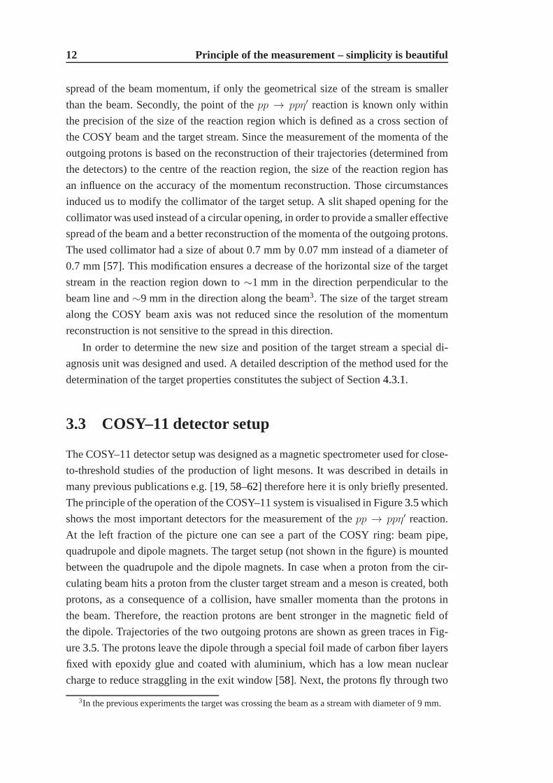
The measured drift time of the electronstdrift can be calculated from a difference
between the time signals from the drift chambers and from theS1 detector. The arrival
times of the signals from those detectors at the Time to Digital Converters (TDC) are
described by following equations:
TDCDC = tDCstop − ttriggerstart TDCS1 = tS1stop − ttriggerstart , (4.2)
wherettriggerstart denotes a common start signal for an event andtistop denotes the stop
signal fromi-th detector, which is a sum of the following terms:
tDCstop = trealDC + tdrift + Ck
DC tS1stop = trealDC +∆tDC−S1 + CS1 , (4.3)
wheretrealDC defines the real time when the particle passes through the drift chamber,
∆tDC−S1 gives the time of flight of the particle between DC and S1,CS1 is a constant
corresponding to the time offset of the S1 detector andCkDC stands for the time offset
of thek-th wire of the drift chamber. The difference between the time signals from the
drift chamber and the S1 scintillator can then be written as:
TDCDC−TDCS1 = tDCstop−ttriggerstart −tS1stop+ttriggerstart = tdrift+Ck
DC −∆tDC−S1 − CS1︸ ︷︷ ︸
Ck
.
(4.4)
TheCk offsets were adjusted based on the leading edge of the drift time spectra (see
Figure4.1). The∆tDC−S1 depends on the particle velocity. However, for protons from

20 First steps on the way to the total width
0
250
500
750
1000
1250
1500
1750
2000
0 100 200 300 400 500 600 700drift time [ns]
cou
nts
Figure 4.1: Typical spectrum of the drift time for a single plane.
thepp → ppη′ reaction (even at the largest access energy (Q = 5 MeV) studied) it varies
only from 0.72 to 0.78 (in speed of light units) and results ina variation of∆tDC−S1
in the order of∼0.3 ns, which can be neglected in view of the 400 ns drift time for
20 mm distance (size of the one cell). The offsets were set foreach plane separately.
This allows to make a single space-time calibration for all cells in one plane.
4.2.1.2 Time-space calibration
The time-space calibration of the drift chamber is a procedure to obtain the dependence
between drift time and the distance of the track to the sense wire. Charged particles
crossing the drift chamber cause gas ionisation and generate electron clusters moving
towards the anode wires. The drift time of those electron clusters (t) can be transformed
to the minimum distance between the trajectory of a particlecrossing the drift chamber
and the sense wire (d). The relation between drift time and the minimum distance
(d(t)) has to be derived from the experimental data and, to minimise the influence of
variations like atmospheric pressure, air humidity and gasmixture changes [65] on the
drift velocities, it should be determined separately for different periods of data taking.
In this analysis∼22-24 hours periods were used.
The calibration method is based on the assumption that the trajectory of a particle
crossing the drift chamber is a straight line. Starting withthe approximate time-space
functiond(t)3 the minimum distance between trajectory and the sense wireswere cal-
culated. Then, a straight line was fitted to the obtained set of points. The minimum
3As the approximate calibration a function determined in theprevious experiment was used. In gen-
eral one can extract the space-time relation from the shape of the drift time distribution using the "uni-
form irradiation" method [66, 67].
4.2 Calibration of detectors 21
distance between the fitted line and the sense wire fori-th event is denoted asdfiti (t).
The correction∆d(t) of the approximate time-space functiond(t) has been calculated
as a function of the drift timet from the following equation:
∆d(t) =1
n
n∑
i=1
(di(t)− dfiti (t)) , (4.5)
wheren denotes the number of entries in the data sample. Then the newcalibration
function was calculated as:
dnew(t) = d(t)−∆d(t) . (4.6)
The above procedure was repeated until∆d(t) became negligible in comparison to the
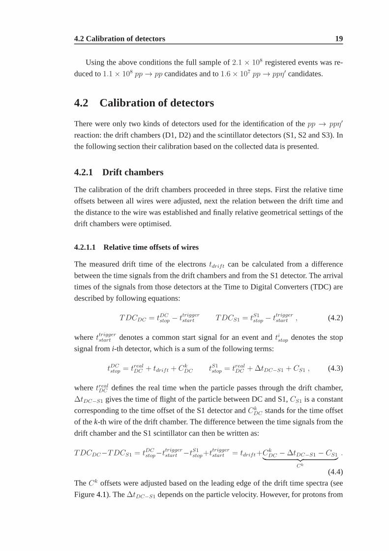
spatial resolution of the chamber. An example of the calculated time-space function
for an arbitrarily chosen sense wire in DC1 is presented in Figure4.2(left). In the right
plot, for an arbitrarily chosen plane of DC1, the middle linecorresponds to the average
difference∆d(t) while the upper and lower lines denote one standard deviation of the
(di(t) − dfiti (t)) distribution. As can be inferred from the right plot of Figure 4.2 the
achieved spatial resolution amounts to about 100µm over the whole drift time range
except for the small area very close to the sense wire.
0
0.25
0.5
0.75
1
1.25
1.5
1.75
2
0 100 200 300 400 500 600 700driff time + offset [ns]
dis
tan
ce [c
m]
-0.05
-0.04
-0.03
-0.02
-0.01
0
0.01
0.02
0.03
0.04
0.05
0 100 200 300 400 500 600 700 800driff time [ns]
∆d(t
) [c
m]
Figure 4.2: Left: Distance from the particle trajectory to the sense wire as a function
of the drift time.Right: Average deviation∆d(t) between the measured and the fitted
distances of tracks from the sense wire as a function of the drift time as obtained after
the second iteration (see text). The distribution around∆d = 0 corresponds to the
correction∆d(t) and the lines around±0.01 cm denote one standard deviation of the
(di(t)− dfiti (t)) distribution.

22 First steps on the way to the total width
4.2.1.3 Relative positions of the drift chambers
The relative geometrical setting of the drift chambers was established based on the
quality of the fit of a straight line to the distances of the particle trajectory to the sense
wires in both drift chambers. The idea of the method is schematically presented in Fig-
ure4.3. Based on theχ2 distribution of the fit the relative position of the chamberswas
found to be∆x = 1.4 mm,∆y = −1.8 mm and∆z = 0.5 mm (the statistical errors
are negligible). Typical spectra of theχ2 values for X and Y directions are presented in
Figure4.4. The larger absolute changes ofχ2 for variations of the∆X than for the∆Y
DC1
DC2
DC1
DC2
DC1DC1
DC2 DC2
Figure 4.3: The idea of the derivation of the relative position of the drift chambers.
From left to right: (top view of the drift chambers pairs) a charged particle crosses two
drift chambers (trajectory plotted as cyan arrow); positions of the trajectory (green) in
each plane (derivation based on the calibration); straightline (blue) fitted to position
information from the drift chambers, in case when the relative position of the drift
chambers is known correctly; the same as before but in case when there is a discrepancy
between nominal and real position of the detectors.
1
1.5
2
2.5
3
3.5
4
-1 -0.5 0 0.5 1DC2 shift in X [cm]
χ2 /nfr
ee
0.88
0.9
0.92
0.94
0.96
0.98
1
1.02
-1 -0.5 0 0.5 1DC2 shift in Y [cm]
χ2 /nfr
ee
Figure 4.4: Value of reducedχ2 for the fit of the straight line to the signals from both
drift chambers as a function of their relative position in X (left) and Y (right) direction.

4.2 Calibration of detectors 23
direction correspond to the better spatial resolution of the drift chambers in X direction
compared to the Y direction. This is due to the construction of the planes with wires
oriented both vertically and inclined by±31◦ [58].
After the relative adjustment of the drift chambers, their position with respect to the
dipole was established based onpp → pp events. Details are presented in Section4.3.2.
4.2.2 Timing of scintillator detectors
The detectors S1 and S3 used for particle identification in the time-of-flight method
were calibrated in order to adjust time offsets for particular photomultipliers (PM). S1
consist of 16 scintillating modules read out by photomultipliers on both sides, while
S3 is a scintillator wall read out by a matrix of 217 photomultipliers. The time-of-
flight is defined as the difference between times of crossing the S1 and S3 detectors
(ToF = tS3 − tS1). For the calibration of the scintillator counters we compare the
time-of-flight obtained from signals registered in the S1 and S3 detectors and the time-
of-flight calculated from the reconstructed momentum of theparticle.
The experimentally available TDC values depend on the time when a particle
crosses the detectors(tS1, tS2) plus the propagation time of the created light and elec-
trical signals. In general, it may by expressed as:
TDCS1(PM) = tS1 + t(y) + twalkS1 (PM) + toffsetS1 (PM)− ttrigger
TDCS3(PM) = tS3 + t(l) + twalkS3 (PM) + toffsetS3 (PM)− ttrigger, (4.7)
wherettrigger denotes the time of the trigger signal,t(y) denotes the time of light prop-
agation for the distance between the cross point in the S1 module and the scintillator
edge andt(l) stands for the time of light propagation for the distance between the hit
position in S3 and the photomultiplier. Due to the usage of leading edge discriminators
a time walk effectis present, i.e. a variation of the registered TDC timetwalk(PM) as
a function of the signal amplitude. The correction of this effect can be done by ap-
plying the formulatwalk(PM) ≈ constant × (ADC)−1
2 , whereADC denotes the
signal charge value [68]. Since thettrigger values are the same in both equations4.7for
computation ofToF only time offset valuestoffset(PM) are unknown. However, they
can be obtained by a comparison of theToF value based on the signals from scintilla-
torsToFS1−S3 and the time-of-flight value calculated from the reconstructed particle
momentumToFmom = l/β, wherel is the path length between the S1 and the S3 de-
tectors obtained from the trajectory reconstructed in the drift chambers, andβ is the
particle velocity calculated from the reconstructed momentum with the known mass,
with the identification of the particle based on the invariant mass distribution result-
ing with time offsets determined in former experiments. Having approximate values of

24 First steps on the way to the total width
toffsetS1 (PM) the time offsets for the photomultipliers in the S3 detectorcan be deter-
mined. Then, using the determined values oftoffsetS3 (PM) the new set oftoffsetS1 (PM)
can be calculated. After a few iterations the offsets for both detectors were obtained.4.
As an example the plots in Figure4.5present results of the calibration for arbitrarily
chosen photomultipliers (PM) of the S1 and S3 detectors.
0
2000
4000
6000
8000
10000
12000
14000
-6 -4 -2 0 2 4 6time offset for 3rd mod S1 [ns]
cou
nts
-2
-1.5
-1
-0.5
0
0.5
1
1.5
2
210 212 214 216 218 220ID of S3 PM
tim
e o
ffse
t [n
s]
Figure 4.5: Distributions of the difference determined from the time-of-flight mea-
sured between the S1 and the S3 detectors and the time-of-flight calculated from the
momentum reconstructed based on the curvature of the trajectory in the magnetic field.
As an example spectra for the 3rd S1 module and an exemplary range of photomul-
tipliers (PM) of the S3 detector are shown. The counting rateof PM 210 and 219 is
smaller since these photomultipliers are positioned at theedges of the detector.
4.3 Properties of the cluster target stream
Since the momentum determination of the outgoing particlesis based on the track re-
construction to the centre of the reaction region (for details see Section5.1), the size
and position of the target stream influence the experimentalmomentum reconstruction
significantly, and the accuracy of their determination willreflect itself in the determina-
tion of systematic uncertainty of the resolution of the missing mass spectra. Therefore,
the properties of the cluster target were monitored via two independent methods: using
a dedicated diagnosis unit and inspecting a kinematic ofpp → pp events.
4In case of the S1 detector, further on in the analysis of thepp→ ppη′ reaction the average of times
from upper and lower photomultipliers were used.

4.3 Properties of the cluster target stream 25
4.3.1 Diagnosis unit – wire device
The diagnosis unit was developed for the measurement of the position and size of the
target stream. Figure4.6 presents a photo of the tool. As shown schematically in the
left part of Figure3.4 it was installed above the reaction region downstream the target
beam5, allowing for the monitoring of the size and position of the target concurrently
to the measurements of thepp → ppη′ reaction.
Figure 4.6: Photography of the diagnosis unit. For the description see text.
The monitoring of the target properties above the beam line permits to interpo-
late the target position and size to the reaction region taking into account the distance
between collimator and reaction region (∼59 cm), and the distance between reaction
region and diagnosis unit (∼71 cm).
The diagnosis unit (shown in Figure4.6) consists of threearms: two wires with
diameters of 1 mm and 0.1 mm (hardly visible in the photo) and abroadarm, the part
with holes and three short perpendicular wires6.
During the measurement the diagnosis unit rotates with constant angular velocity
around the axis perpendicular to the target stream. Thearmscross the target stream
one by one, which cause changes of the pressure in the stage above the diagnosis unit
(see the left part of Figure3.4). The measured pressure values are presented in the
upper left part of the Figure4.7 as a function of time. The sixfold structure visible
in the plot corresponds to the differentarmsof the diagnosis unit crossing the target
stream (eacharm crosses the stream twice during a full rotation, once at the top and
5As shown in the left part of Figure3.4the target stream moves from the bottom to the top.6The usage of three perpendicular wires allowed for the determination of the target inclination.

26 First steps on the way to the total width
0
0.5
1
1.5
2
2.5
3
0 1000 2000 3000time [a.u.]
bea
m p
ress
ure
du
mp
[a.u
.]
0.5
1
1.5
2
2.5
3
1500 1550 1600 1650time [a.u.]
bea
m p
ress
ure
du
mp
[a.u
.]
1
1.25
1.5
1.75
2
2.25
2.5
2.75
3
2200 2250 2300time [a.u.]
bea
m p
ress
ure
du
mp
[a.u
.]
2
2.1
2.2
2.3
2.4
2.5
2.6
2.7
2.8
2.9
3
1240 1260 1280 1300 1320 1340time [a.u.]
bea
m p
ress
ure
du
mp
[a.u
.]
Figure 4.7: Example of changes of the target stream pressureas a function of the
rotation time of the diagnosis unit (black). Red lines correspond to the result of the
simulation.Upper left: Full cycle of the rotation.Upper right: Close-up of the mini-
mum due to thebroadarm and three short wires.Lower: Close-ups of the minima due
to the thick (lower left) and thin (lower right ) wire passage. The width of theplateau
at the top of the pictures corresponds to the pressure fluctuations.
a second time at the bottom). The rotation was realised by a step motor and the full
rotation cycle took 2400 steps. The first structure in the upper left part of the Figure4.7
corresponds to the passage of the broadarm with three perpendicular wires (the small
stepat the leading edge) and the part with holes (the double-wellstructure). The next
two sharp minima correspond to the crossing of the thick and thin wire, respectively.
The amplitudes of the minima differ slightly depending whether thearm crosses the
stream closer to or further from the pressure measurement region. The remaining plots
in Figure4.7contain close-ups of structures from the upper left part.
The decrease of the measured pressure is proportional to thearea of the wire block-
ing at a given moment the stream of the target. Therefore, knowing the size of the
particular parts of the diagnosis unit and velocity of the rotation one can simulate the
relative changes of the pressure as a function of time, underthe assumption of the pa-

4.3 Properties of the cluster target stream 27
rameters describing the size, inclination (angle) and position of the target stream. The
comparison of the results of simulations with the measured variations of the pressure
allows to establish the parameters of the target based on theminimialisation of theχ2.
The red lines in the plots in Figure4.7 denote result of the simulation corresponding
to the parameters for which theχ2 is at a minimum value. The determined properties
of the target stream in the reaction region are:
width = (0.089± 0.005) cm
length = (1.053± 0.005) cm
X − position = (0.27± 0.05) cm (4.8)
Z − position = (0.02± 0.05) cm
angle = (4.03± 0.01) deg,
where the position is calculated in the nominal target system reference frame and the
angle is defined with respect to the beam direction. The quoted uncertainties of X and
Z positions include the inaccuracy of the determination of the position of the diagnosis
unit in the reference frame of the target. Size and relative position of beam and target
stream are shown in Figure4.8.
COSYbeam
4o
clustertarget
0.9mm
11m
m
Figure 4.8: Size and relative position of beam and target stream determined from the
measurement based on the diagnosis unit. (In this thesis a Z coordinate is defined along
the COSY beam line.)
There were no changes of the target stream size, angle and X-position during the
entire experimental period. However, there were changes ofthe Z position in the order
of 1 mm. A quantitative discussion of this variations is presented in Section4.3.3.
It is worth to stress that the target stream width, length andangle correspond to an
effective target width of 1.06 mm.

28 First steps on the way to the total width
4.3.2 Kinematic ellipse frompp → pp events
The second and independent method used for the determination of the target stream
properties is based on the measurement of the momentum distribution of elastically
scatteredpp → pp events.
Elastically scattered protons form an ellipsoid in momentum space in the LAB sys-
tem. The projection of the momentum components (p⊥ = perpendicular, p‖ = parallel
to the beam direction) constitutes an ellipse. The acceptance of the COSY–11 detector
allows for the measurement of the lower right part of it (see left part of Figure4.9).
0
200
400
600
800
1000
1200
1400
1600
x 10 2
-0.3 -0.2 -0.1 -0 0.1 0.2 0.3distance to ellipse [GeV/c]
cou
nts
0
500
1000
1500
2000
2500
x 10 2
-0.3 -0.2 -0.1 -0 0.1 0.2 0.3distance to ellipse [GeV/c]
cou
nts
Figure 4.9: Upper left: Part of the experimental kinematic ellipse frompp → pp
events analysed for the nominal target stream position (x = 0, z = 0). The smooth
change of the amplitude of the density distribution reflectsthe strong angular depen-
dence of thepp → pp cross section. Theoretical ellipses for beam momentum values
3211 MeV/c (nominal one) and 3111 MeV/c are plotted as blue and green lines, re-
spectively.Upper right: Projection of the distribution from upper left plot along the
theoretical blue ellipse.Lower left: The same data as for upper left plot but analysed
for a target stream position of x = 2.35 mm, z = 0.Lower right: Projection of the
distribution from lower left plot along the theoretical blue ellipse.

4.3 Properties of the cluster target stream 29
The momentum reconstruction of positively charged particles in the COSY–11 detec-
tor is based on the determination of their trajectories by means of the drift chambers
and the back-reconstruction through the known magnetic field to the reaction region
(see Figure3.6). Since the exact reaction point is known only with an accuracy deter-
mined by the size of the reaction region, defined as the overlap of the beam and the
target stream, back-reconstruction is performed to the centre of this region. This causes
the spread of the points around the calculated kinematic ellipse. Naturally the spread
depends on the size of the reaction region, whereas the average shift of the points from
the expected ellipse reflect a wrong assumption of the position of the centre of the re-
action region. In principle the average shift may also be dueto a wrong assumption
of the absolute value of the beam momentum. However, as proven already in the pre-
vious analysis [69] it may by safely neglected taking into account the accuracyof the
absolute beam momentum determination of 3 MeV/c [70]. For the illustration of the ef-
fect, the nominal beam momentum was decreased by 100 MeV/c (see Figure4.9). One
can estimate that an inaccuracy of 3 MeV/c would cause a negligible effect. The blue
line denotes the expected ellipse for the nominal beam momentum of 3211 MeV/c,
the green line for 3111 MeV/c. The projection of the experimental points along the
expected ellipse (blue line) is presented in the upper rightplot in Figure4.9.
Moreover, the momentum reconstruction is very sensitive tothe assumption of the
centre of the interaction region. The ellipse presented in the upper left plot in Figure4.9
was derived under the assumption that the target stream is atthe nominal position
(x = 0, z = 0, the y-position is well defined by the plane of the circulating beam).
The ellipse in the lower left plot in Figure4.9was derived from the same data as for
the ellipse from upper plot, however, the analysis was performed under the assumption
of the target centre position: x = 2.35 mm, z = 0. The blue theoretical ellipse follows
the shape of the data, much better than for the (wrong) x = 0 position, which is also
visible in the projection in the lower right plot in Figure4.9.
The value of the reconstructed momentum depends also on the assumed relative
settings of the drift chambers, dipole magnet and the target. Therefore the momentum
distributions of thepp → pp events are also sensitive to the drift chamber position rela-
tive to the dipole. However, wrong assumption about the position of the drift chambers
or about the position of the target modify those distributions in a different ways and
therefore these positions can be established independently of each other.
To reduce the background contribution from the multibody production reactions
two cuts were applied. First the squared missing mass to thepp → pX reaction was
calculated and then the range of the squared missing mass from 0.4 to 1.2 GeV2/c4
was chosen for proton selection (see left plot in Figure4.10). In addition, the two-
body kinematics of elastic proton-proton scattering allows to combine the scattering
anglesΘ1 andΘ2 of the recoiled and forward flying protons. In the COSY–11 apparatus

30 First steps on the way to the total width
0
1000
2000
3000
4000
5000
6000
x 10 2
0 0.5 1 1.5 2 2.5 3 3.5missing mass2 [GeV2/c4]
cou
nts
10
15
20
25
30
35
40
45
30 35 40 45 50 55 60 65 70 75 80X position in S1 [cm]
elem
ent
ID o
f S
i
Figure 4.10: Left: Square of the missing mass to thepp → pX reaction. A clear
signal from the protons is visible. The blue dashed lines correspond to the applied
cut. Right: Correlation between position of the registered particle inthe S1 detector
and the element number of the Si detector (see Figure4.11). The blue dashed lines
correspond to the cut range. The relative intensity increases in channels 24 and 27 of
the Si detector are due to higher noise levels in these detector elements.
21
BEAM
DIPOLE
BEAM
CLUSTER TARGET
B
VACUUM CHAMBER
EXIT WINDOW
SiS4
D1
D2
S1
3
16
12348
80
60
-80
θ1
X [cm]
S1
θ2
Figure 4.11: Close-up of the part of the COSY–11 detector used for the registration of
elastically scattered events. The picture is adapted from [18].

4.3 Properties of the cluster target stream 31
the scattering angles correspond to the pad number of the silicon monitor detector
(Si) and the position in the S1 detector (see Figure4.11). The correlation is visible
in the right plot in Figure4.10. The cut was applied as indicated by the blue dotted
lines. The applied cuts are tight, however, the absolute number ofpp → pp events is
not substantial for theΓη′ analysis. The kinematic ellipse and its projection along the
theoretical curve with adjusted position of the target after applying the mentioned cuts
is presented in Figure4.12. A negligible amount of background remained.
0
250
500
750
1000
1250
1500
1750
2000
2250
x 10 2
-0.3 -0.2 -0.1 -0 0.1 0.2 0.3distance to ellipse [GeV/c]
cou
nts
Figure 4.12:Left: Experimental kinematic ellipse frompp → pp events analysed for
the corrected position of the target and drift chambers after application of the cuts on
the squared invariant mass and angles correlation spectra.The theoretical ellipse for
the nominal value of the beam momentum is plotted as a blue line.Right: Projection
of the distribution from left plot along the theoretical ellipse.
The simultaneous comparison of the theoretical ellipses with the experimental ones
derived for five different beam momenta allows for the determination of position and
effective width of the target and position of the drift chambers. The effective target
width has an influence on the spread of points around the kinematic ellipse. However,
in practise, based on the elastically scattered events one can determine the target width
only if it is greater than∼ 0.2 cm (as it is shown in Figure4.13). Below 0.2 cm other
effects dominate the contribution to the spread of the experimental points. The obtained
results using the described method are:
effective target width < 0.2 cm,
target X − position = (0.235± 0.001) cm,
drift chamber 1 absolute position = (0.62± 0.01) cm, (4.9)
drift chamber 2 absolute position = (0.76± 0.01) cm,
drift chamber angle = (0.045± 0.005) deg.

32 First steps on the way to the total width
80
100
120
140
160
180
200
220
240
0 0.1 0.2 0.3 0.4 0.5 0.6 0.7 0.8 0.9 1effective target width [cm]
FW
HM
of
kin
emat
ic e
llip
se [M
eV]
Figure 4.13: Simulated dependence of the distribution width (FWHM) of the projec-
tion along the kinematic ellipse on the effective target width.
The obtained target position and effective size are in the good agreement with the
values derived from the measurement with the diagnosis tool.
4.3.3 Density distribution of the cluster target stream
Figure4.14shows the changes of the average distance between the theoretical ellipse
and the experimental distribution as a function of time. These variations correspond to
changes of the centre of the density distribution of the target and hence influence the
resolution of the missing mass. As an example of the effect, the missing mass spectra
for thepp → ppX reaction obtained for the first and second half of the measurement at
3211 MeV/c momentum are presented in Figure4.15, where the first part of the mea-
surement (from∼100 h to∼175 h) corresponds to the large variation of the kinematic
ellipse position, while the second part (from∼175 h to∼250 h) to the small variations.
The presented spectra differ and theη′ signal is better visible in the data collected in
the period with smaller variations (a detailed descriptionof the missing mass technique
will be presented in section5.3). Such fluctuations could be explained by variations of
the beam momentum due to the changes of the beam optics7 or by small fluctuations
of the density distribution of the target stream. However, the beam optics variation is
excluded by the results of the monitoring of the stability ofthe COSY beam (as de-
scribed in the next section). The observed variations of thekinematic ellipse position
can be plausibly explained by density changes inside the target stream in beam direc-
tion. In this direction the target length is about 1 cm (see section 4.3.1) and expected
fluctuations of the density can cause the changes of the centre of the target stream
distribution in the order of 1 mm. Such variations along the z-axis were observed by
7The variations of the beam optics could be caused by e.g. the variations of the dipole currents, or
small deformation of the dipole shape caused by temperaturechanges.

4.3 Properties of the cluster target stream 33
0.016
0.018
0.02
0.022
0.024
0.026
0.028
0.03
0 100 200 300 400 500time [h]
dis
tan
ce t
o e
llip
se [G
eV/c
]
-0.006
-0.004
-0.002
0
0.002
0.004
0.006
0 100 200 300 400 500time [h]
dis
tan
ce t
o e
llip
se [G
eV/c
]
Figure 4.14:Left: Distance between the theoretical ellipse and the experimental dis-
tribution for the elastic kinematics plotted as a function of time. Points denote results
averaged over∼2 hours. Solid lines denote succeeding days of the measurement, while
the dashed lines separate periods with different beam momenta (3218, 3211, 3214,
3213 and 3224 MeV/c). The values are not around 0 since at thisstage the analysis
was performed without corrections for the target and drift chamber positions as de-
scribed in the previous section. The four days gap after∼300 hour of measurement
time is due to a cyclotron down time.Right: The same data as presented on the left
plot but analysed after correction of the changes of the centre of the density inside the
target stream (see text for the details). Both plots have thesame scale on the vertical
axis.
0
5
10
15
20
25
30
35
40
45
0.956 0.958 0.96missing mass [GeV/c2]
even
ts/1
00ke
V
0
5
10
15
20
25
30
35
40
45
0.956 0.958 0.96missing mass [GeV/c2]
even
ts/1
00ke
V
Figure 4.15: Missing mass spectra extracted from data collected for 3211 MeV/c beam
momentum.Left: Result from∼100 h to∼175 h of the experiment.Right: Result
from∼175 h to∼250 h of the experiment.

34 First steps on the way to the total width
means of the diagnosis unit as mentioned in Section4.3.1. Therefore, in the following
analysis we assumed that the observed deviations are due to the target density vari-
ations and corrected them by continuous changes of the nominal value of the centre
of the target along the z direction (see Figure4.16). The corrections were interpolated
between points calculated for each∼2 hours interval of beam time. The average dis-
tance to the expected kinematic ellipse after the correction for target density fluctuation
is presented in the right panel in Figure4.14. The first two days of the measurement
were used for different test of the detection system and the optimisation of the beam
optics which cause somewhat larger fluctuations during thisperiod. Therefore the data
collected during those two days were not used for the finalΓη′ determination.
-0.06
-0.04
-0.02
0
0.02
0.04
0.06
-1 -0.5 0 0.5 1target position in Z direction [cm]
dis
tan
ce t
o e
llip
se [G
eV/c
]
Figure 4.16: Average deviation of the experimental points distribution from the ex-
pected kinematic ellipse as a function of target position inthe direction parallel to the
COSY beam.
4.4 Monitoring of the stability of the proton beam
Although the frequency of the circulating beam is monitoredroutinely several times
per minute, during the described experiment a measurementsof additional parameters
were performed in order to provide a better control of the stability of the proton beam.
4.4.1 Synchrotron parameters
The standard technique for monitoring the beam momentum at the COSY accelerator
is the measurement of the frequency distribution of the circulating beam. Based on the

4.4 Monitoring of the stability of the proton beam 35
equation [52, 70, 71]:f − f0f0
= ηbeamp− p0p0
, (4.10)
wheref denotes the frequency andp denotes the beam momentum, (f0 andp0 corre-
spond to their nominal values, respectively) one can transform the frequency into the
beam momentum. (The determination of the real value of the beam momentum is de-
scribed in section5.4.) Theηbeam parameter depends on the settings of the accelerator
and for the described measurement was equal to−0.10 ± 0.01 [70]. As an example
a spectrum transformed to the momentum coordinate for the lowest beam energy used
in the experiment is presented in Figure4.17. The beam momentum distribution is
smooth and its spread is equal to 2.5 MeV/c (FWHM). However, due to the position of
the COSY–11 target system in a bending section of the COSY ring in a dispersive re-
gion, the effective spread of the beam (the momentum rangeseenby target) is smaller.
The dispersion relation is:
∆x = D∆p
p0, (4.11)
where∆x and∆p denote the difference between the real and nominal values ofparticle
orbit and momentum, respectively. The dispersion in the COSY–11 target system was
set toD = 14.15 m, which (taking into account the 1.06 mm effective target width)
results in an effective beam spread of±0.06 MeV/c. The relevant momentum range is
marked by blue lines in Figure4.17.
0
20
40
60
80
100
3.2075 3.21 3.2125 3.215pbeam [GeV/c]
cou
nts
Figure 4.17: Example of the momentum spectrum for the measurement with the nomi-
nal beam momentum of 3211 MeV/c. The dashed lines limit the effective spread of the
beam due to the dispersion relation for a target width of 1 mm (blue) and 1 cm (green).
After variations of the position of the kinematic ellipse have been observed during
anon-lineanalysis, measurements of additional (to the frequency spectrum) parame-
ters were implemented. To check the stability of the beam optics the current through

36 First steps on the way to the total width
the dipole magnets was controlled, however, no fluctuationson the level of10−5 during
beam cycles were found. Furthermore the temperatures of theincoming and outgoing
water used for the magnets cooling were monitored8 – also without any correlations
with the observed behaviour of the ellipse position.
4.4.2 Atmospheric conditions
In addition to the control of the hardware status, the atmospheric conditions were moni-
tored inside and outside the COSY-tunnel. Thermograph and hygrograph were installed
in the COSY tunnel close to the COSY–11 detector and information about air temper-
ature, pressure and humidity outside the building were delivered by the meteorology
station (courtesy of Dr. Axel Knaps). No correlations to theobserved behaviour of the
kinematic ellipse was found.
The stability of the parameters described in this and the previous sections raised
our confidence that the fluctuations of the kinematic ellipseposition was due to the
density fluctuation inside the target stream.
8The variation of the temperature could cause changes of the dipole dimensions and hence changes
of the magnetic fieldshape.

Chapter 5
Identification of the pp → ppη′ reaction
The identification of protons via the invariant mass method and the determination of
missing masses of unregistered particles allow to selectpp → ppη′ events.
5.1 Identification of the outgoing protons
The invariant mass of registered particles was calculated from the equation:
m2
inv =p2(1− β2)
β2, (5.1)
where momentump and velocityβ of the particle were determined by means of drift
chambers (track reconstruction through the known magneticfield) and the S1-S3 ho-
doscope (ToF), respectively. The correlations of the two invariant masses for events
with two reconstructed tracks are presented in Figure5.1. Appropriately chosen cuts
allow to select events corresponding only to two registeredprotons.
Figure 5.1: Distribution of the invariant mass of two registered particles. The super-
imposed black dashed square represents the applied cut. Outside the selected areaπ+p
andpπ+ events are visible. Note that the number of entries is given in the logarithmic
scale.

38 Identification of the pp → ppη′ reaction
5.2 Determination of the relative beam momenta
Due to the inaccuracy of the orbit length [70], the COSY crew can set the absolute
momentum of the beam (nominal value) only with an accuracy of3 MeV/c. Since
this was not sufficient for our experiment, we decided to use collectedpp → ppη′
andpp → pp events for the determination of the absolute beam momenta. Based on
the position of theη′ signals in the missing mass spectra the absolute beam momenta
can be derived. For this procedure the mass of theη′ meson has to be determined as
will be discussed later. Since, on the other hand, the correct signal position can be
obtained only for a background-free missing mass spectrum,the background has to be
subtracted first. The method used for the background subtraction (see the next section)
requires information about the relative beam momenta, which can be determined by the
comparison of kinematic ellipses frompp → pp events (see Section4.3.2). Although
the position of the kinematic ellipse depends stronger on the target position than on
the beam momentum (see Section4.3.2) it can be used for calculations of the relative
beam momenta, since the fluctuations during the measurementwere corrected before.
As a result we obtained the following momenta relative to thelowest measured one:
∆p1−2 = 1.85± 0.01 MeV/c
∆p1−3 = 2.82± 0.01 MeV/c
∆p1−4 = 6.53± 0.01 MeV/c
∆p1−5 = 12.66± 0.01 MeV/c
5.3 Missing mass spectra and background subtraction
The determined missing mass spectra of the five measured energies were used (i) to
determine the background, (ii) to evaluate the absolute beam momenta and (iii) to
calculate the width of theη′ meson (see next chapter).
5.3.1 Experimental background from different energies
The missing mass spectrum of the multipion background can beestablished either by
Monte Carlo simulations (see e.g. [60]) or by the usage of the experimental background
collected for another energy [72]. The second method was used in the analysis and is
described in this dissertation, since it allows to avoid additional approximations and
assumptions.
The used background subtraction method was described in detail in article [72].
It is based on the observation that the shape of the multipionmass distribution does not
change when the excess energy for thepp → ppη′ reaction varies by a few MeV only

5.3 Missing mass spectra and background subtraction 39
since the dominant background originates from2π and3π production [40] and the ex-
cess energy for either of these reactions is larger than 0.5 GeV. Figure5.2demonstrates
that the change in the shape of the missing mass distributions is in the order of 1% over
a range more than 0.2 GeV and in this experiment a range of about 0.005 GeV is impor-
tant. From the measurement below the threshold for theη′ production, the signal-free
background can be obtained and used for the close-to-threshold production process.
Also the measurements sufficiently high above the threshold, with an excess energy
larger than the resolution of the missing mass determination, provides a signal-free
background for close-to-threshold production data.
Cou
nts
Missing mass [ GeV/c2 ]
dm
dNπ(Qη’ = 20)
dm
dNπ(Qη’= 0, shifted)
Missing mass [ GeV/c2 ]
Sys
tem
atic
al e
rro
r [
% ]
Figure 5.2:Upper: Missing mass distribution with respect to thepn system calculated
from Monte Carlo data for thepn → pnππ process for a beam energy at the threshold
(dotted line) and 20 MeV above the threshold for thepn → pnη′ reaction (solid line).
The dotted histogram was shifted by 20 MeV.Lower: Difference between the spectra
in the upper plot normalised to the solid line, which gives the systematical error due to
the background determination. The plots are adapted from [72].

40 Identification of the pp → ppη′ reaction
The excess energy in the centre of mass system (CM) is defined as:
Q =√s−
N∑
i
mi , (5.2)
where√s denotes the centre-of-mass total energy of the colliding protons system and
N is the number of outgoing particles. In order to determine the background shift be-
tween the spectra the relative values of Q have to be known. Since Q depends inter
alia on the beam momentum from which the relative changes canbe controlled via
the position of the experimental distributions of the kinematic ellipse, relative Q val-
ues can be obtained. Missing mass spectra for thepp → ppX reaction obtained for
the lowest (3211 MeV/c) and highest (3224 MeV/c) beam momenta in the described
experiment are presented in Figure5.3. It is important to stress that the background
distribution is smooth in the whole range studied. The spectrum for the beam momen-
tum of 3224 MeV/c was shifted according to the described method and normalised to
the data from lower energy. As one can see the background shape in the signal-free
region is the same with respect to the statistical errors forboth energies. This confirms
the correctness of the above described method for background determination.
0
25
50
75
100
125
150
175
200
225
0.95 0.9525 0.955 0.9575missing mass [GeV/c2]
even
ts/1
00ke
V
Figure 5.3: Missing mass spectra for thepp → ppX reaction. Red points correspond to
the measurement at 3211 MeV/c beam momentum (the lowest one in the described ex-
periment), while black ones represent the measurement at the highest beam momentum
(3224 MeV/c). The black points were shifted by the difference between the kinematic
limits and normalised to the red points (see text for details).
5.3.2 Background parametrisation with polynomial fit
To decrease the influence of the statistical fluctuation of the background and based on
the smooth change of the background in the signal region (seeFigure5.3) the back-
ground for each energy was determined as a second order polynomial which was de-
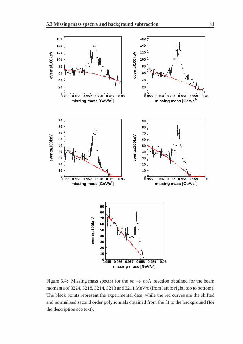
5.3 Missing mass spectra and background subtraction 41
0
20
40
60
80
100
120
140
160
0.955 0.956 0.957 0.958 0.959 0.96missing mass [GeV/c2]
even
ts/1
00ke
V
0
20
40
60
80
100
120
140
160
0.955 0.956 0.957 0.958 0.959 0.96missing mass [GeV/c2]
even
ts/1
00ke
V
0
10
20
30
40
50
60
70
80
90
0.955 0.956 0.957 0.958 0.959 0.96missing mass [GeV/c2]
even
ts/1
00ke
V
0
10
20
30
40
50
60
70
80
90
0.955 0.956 0.957 0.958 0.959 0.96missing mass [GeV/c2]
even
ts/1
00ke
V
0
10
20
30
40
50
60
70
80
90
0.955 0.956 0.957 0.958 0.959 0.96missing mass [GeV/c2]
even
ts/1
00ke
V
Figure 5.4: Missing mass spectra for thepp → ppX reaction obtained for the beam
momenta of 3224, 3218, 3214, 3213 and 3211 MeV/c (from left toright, top to bottom).
The black points represent the experimental data, while thered curves are the shifted
and normalised second order polynomials obtained from the fit to the background (for
the description see text).

42 Identification of the pp → ppη′ reaction
rived from data at a different energy and was shifted and normalised to the actual data.
The full procedure for background determination consists of the following steps:
1. fit of a second order polynomial to the missing mass spectrum in the signal-free
region for a lower/higher beam energy;
2. shift of the obtained curve according to the calculated Q difference;
3. normalisation of the curve to the data obtained for the actual beam energy.
The results are presented in Figure5.4. The determined curves agree well with the
background data within the statistical accuracy.
5.4 Absolute beam momentum determination
The knowledge of the relative beam momenta (see Section5.2) and the background
shape (see previous section) allows to determine the absolute beam momenta based on
the position of theη′ signal. The procedure relies on the comparison of the position
of theη′ signal with theη′ mass1. Due to the best signal-to-background ratio and the
sharpest signal, for the derivation of the absolute value ofQ, the missing mass ob-
tained for the lowest beam momentum was used, while the otherfour beam momenta
were adjusted with respect to the relative differences obtained in Section5.2. Table5.1
presents the values of the nominal and real beam momenta and corresponding real Q
values. For all measurements the real beam momentum is lowerby about 0.5 MeV/c.
beam momentum[MeV/c] real excess energy
nominal real [MeV]
3211 3210.7 0.8
3213 3212.6 1.4
3214 3213.5 1.7
3218 3217.2 2.8
3224 3223.4 4.8
Table 5.1: Nominal and real beam momenta for the measurementof thepp → ppη′
reaction and corresponding real values of excess energy.
The accuracy of the real beam momentum derivation depends onthe accuracy of both
the knowledge of theη′ mass as well as determination of the relative beam momenta.
The first component is of systematic type and contributes as an error of±0.2 MeV/c
whereas the second one is of statistical nature and its contribution is negligibly small.
1mη′ = (957.78± 0.06) MeV/c2 [3]

5.4 Absolute beam momentum determination 43
The systematically lower value of the real beam momentum of about 0.5 MeV/c
matches well with the range of accuracy in beam momentum setup being typically
±3 MeV/c [70] and the results are in line with previous experiences at COSY where
also the real beam momentum was smaller than the nominal one [63, 73].

44 Identification of the pp → ppη′ reaction
Chapter 6
Determination of the total width
The determination of the total width of theη′ meson was based on the simultaneous
comparison of all experimental missing mass spectra with the Monte Carlo generated
ones, whereΓη′ was varied in the range from 0.14 to 0.38 MeV.
6.1 Comparison of experimental data with simulations
Thepp → ppη′ reaction and trajectories of the outgoing protons were simulated and
detector signals were generated by the GEANT3-based program [74] for the five in-
vestigated beam energies. The program itself contains the implementation of the whole
geometry of the COSY–11 detector setup. It takes into account also known physical
processes like multiple scattering and nuclear reactions in the detector material, as
well as the detector and target properties established and described in the previous
chapters, like: position and spatial resolution of the drift chambers, size and position
of the target stream and value and spread of the beam momentum.
Afterwards the generated events were analysed in the same way as the experimen-
tal data and sets of missing mass spectra for the five measuredenergies were obtained
for the values ofΓη′ ranging from 0.14 to 0.38 MeV. For simulations of the mass dis-
tribution of theη′ meson the Breit-Wigner formula was used. Finally the Monte Carlo
missing mass spectra with anη′ signal were added to the second order polynomial
fitted to the experimental backgrounds (see Section5.3.2). The obtained spectra were
compared to the experimental ones via calculating theχ2 derived from the maximum
likelihood method [75, 76]. The following formula was used for theχ2 computation:
χ2 = 2
K∑
i=1
[
αNMCi +Bi −Nexp
i +Nexpi ln
(Nexp
i
NMCi +Bi
)]
, (6.1)
whereK denotes the number of bins in the range where the histograms were compared,
α is the free parameter of the fit which describes the normalisation factor of the Monte

46 Determination of the total width
Carlo spectra with theη′ signal. The numbers of entries in thei-th bin in the Monte
Carlo spectra, the background and the experimental spectraare denoted asNMCi , Bi
andNexpi , respectively. The dependence of the calculatedχ2 – quantifying a differ-
ence between the experimental and Monte Carlo spectra – on the appliedΓη′ value is
presented in Figure6.1. The minimum value ofχ2 corresponds toΓη′ = 0.226 MeV,
which is the most likely value of the total width of theη′ meson. The right plot in
Figure6.1 is the close-up of the left plot in the region of the minimum, where the
range of the horizontal axis corresponds to the range whereχ2 differs by one with re-
spect to its minimum value. Since the calculated value ofχ2 is not normalised to the
number of degrees of freedom, the range ofΓη′ whereχ2 = χ2min + 1 corresponds to
the statistical error of the measurement [1, 3, 77], which in case of the reported mea-
surement is±0.017 MeV. The experimental spectra of the missing mass superimposed
with the sum of the background polynomial and the Monte Carlogenerated signals for
Γη′ = 0.226 MeV are presented in Figure6.2. The blue dashed lines mark the range
where the experimental histograms were compared to the result of the simulations. The
presented missing mass signals are the convolution of the total width of theη′ meson
and the experimental resolution.
70
75
80
85
90
95
100
0.15 0.2 0.25 0.3 0.35Γη′ [MeV]
χ2
68.4
68.5
68.6
68.7
68.8
68.9
69
69.1
69.2
69.3
0.21 0.22 0.23 0.24Γη′ [MeV]
χ2
Figure 6.1: Left: Similarity (as a value ofχ2) of the missing mass spectra obtained
from the measurement and from Monte Carlo simulations. The minimum value cor-
responds toΓη′ = 0.226 MeV. Right: Close-up of the left plot with the range where
χ2 = χ2min + 1, which corresponds to the value of the statistical error of the measure-
ment.
The observed dependence of the width of the missing mass signals on the excess
energy (see Figure6.2and6.3) is due to the propagation of errors of protons momenta
involved in the missing mass calculations [49]. Since the Monte Carlo program is re-
producing the changes of the experimental spectra with energy very well, this confirms

6.1 Comparison of experimental data with simulations 47
0
20
40
60
80
100
120
140
160
0.955 0.956 0.957 0.958 0.959 0.96missing mass [GeV/c2]
even
ts/1
00ke
V
0
20
40
60
80
100
120
140
160
0.955 0.956 0.957 0.958 0.959 0.96missing mass [GeV/c2]
even
ts/1
00ke
V
0
10
20
30
40
50
60
70
80
90
0.955 0.956 0.957 0.958 0.959 0.96missing mass [GeV/c2]
even
ts/1
00ke
V
0
10
20
30
40
50
60
70
80
90
0.955 0.956 0.957 0.958 0.959 0.96missing mass [GeV/c2]
even
ts/1
00ke
V
0
10
20
30
40
50
60
70
80
90
0.955 0.956 0.957 0.958 0.959 0.96missing mass [GeV/c2]
even
ts/1
00ke
V
Figure 6.2: The missing mass spectra for thepp → ppX reaction for excess energies
in the CM system equal to 4.8, 2.8, 1.7, 1.4, and 0.8 MeV (from left to right, top to
bottom). Theη′ meson signal is clearly visible. The experimental data are presented as
black points, while in each plot the red line corresponds to the sum of the Monte Carlo
generated signal forΓη′ = 0.226 MeV and the shifted and normalised second order
polynomial obtained as a fit to the signal-free background region for another energy.

48 Determination of the total width
0
20
40
60
80
100
0.955 0.956 0.957 0.958 0.959 0.96missing mass [GeV/c2]
even
ts/1
00ke
V
0
20
40
60
80
100
0.955 0.956 0.957 0.958 0.959 0.96missing mass [GeV/c2]
even
ts/1
00ke
V
-10
0
10
20
30
40
50
60
70
0.955 0.956 0.957 0.958 0.959 0.96missing mass [GeV/c2]
even
ts/1
00ke
V
-10
0
10
20
30
40
50
60
70
0.955 0.956 0.957 0.958 0.959 0.96missing mass [GeV/c2]
even
ts/1
00ke
V
-10
0
10
20
30
40
50
60
70
0.955 0.956 0.957 0.958 0.959 0.96missing mass [GeV/c2]
even
ts/1
00ke
V
Figure 6.3: Background-free missing mass spectra for thepp → ppX reaction for
excess energies 4.8, 2.8, 1.7, 1.4, and 0.8 MeV (from left to right, top to bottom) in
CM system. The experimental data are presented as black points, while the red lines
correspond to the Monte Carlo generated signal forΓη′ = 0.226 MeV.

6.2 Systematic error estimation 49
the correctness of the established detector and target characteristics.
For completeness the experimental missing mass spectra forthe pp → ppX re-
action after background subtraction are presented in Figure 6.3. More than 2300η′
mesons were reconstructed and achieved experimental mass resolution for the lowest
measured energy amounts to FWHM =(FWHM2missing mass− Γ2
η′)1/2 = 0.33 MeV/c2.
6.2 Systematic error estimation
The accuracy of the determination of collected in Table6.1parameters of the COSY–11
detector and the COSY accelerator contribute to the systematic error of the derivation
of theη′ width. The estimated values of the influence of the accuracy of each parame-
ter on the final result are presented. The contributions fromthe accuracy of the target
position and size, the map of the magnetic field, the positionof the drift chambers and
the absolute beam momentum determination were estimated asthe difference between
the derived result of theΓη′ and theΓη′ values established by changing particular pa-
rameter by its error value. The systematic error due to the method of the background
parameter contribution to
the systematic
error[MeV]
map of the magnetic field 0.007
target position 0.006
background subtraction method0.006
ranges of missing mass spectra, whereχ2 was calculated 0.005
bins width 0.004
absolute beam momentum0.003
final state interaction (FSI) between protons0.003
effective target width 0.002
position and orientation of the drift chambers0.001
Table 6.1: Summary of the parameters contributing to the systematic error of theΓη′
measurement at the COSY–11 detector.
subtraction was established as the difference betweenΓη′ values determined using ex-
perimental background shapes from different energies1. The bin width was changed
from 0.1 to 0.04 MeV/c2, while the ranges of the missing mass spectra, whereχ2 was
calculated, were enlarged by 0.7 MeV/c2 at each side (which corresponds to seven bins
1For a missing mass spectrum at a given energy each of four remaining spectra could be used for the
background determination.

50 Determination of the total width
in plot 6.2). The estimation of the influence of the final state protons-proton interaction
is very conservative. The reported value is the difference between the case where the
FSI was and was not taken into account [78, 79].
The total systematic error was calculated as a square root ofthe sum of the squared
values listed in Table6.1and the final result of the measurement of the total width of
theη′ meson conducted with the COSY–11 detector isΓη′ = 0.226 ± 0.017(stat.) ±0.014(syst.) MeV.

Chapter 7
Summary
The aim of this work was to determine the total width of theη′ meson with a unique pre-
cision and independently of the other properties of this meson, like e.g. partial widths
or production cross sections. The motivation for the measurement of the total width
of the η′ meson as well as the experimental method and the final result have been
presented.
The value ofΓη′ was established directly from the measurement of the mass dis-
tribution of theη′ meson. Theη′ meson was produced in proton-proton collisions via
thepp → ppη′ reaction and its mass was reconstructed based on the information about
the momentum vectors of the protons before and after the reaction. The experiment
was conducted in the Research Centre Jülich in Germany. The accelerated and stored
protons were circulating through the stream of the hydrogencluster target in the ring of
the cooler synchrotron COSY. The two outgoing protons were measured by means of
the COSY–11 detector. The reconstruction of a particle trajectory through the known
magnetic field allows for the momentum determination, whilethe ToF method pro-
vides information about the velocity. The identification ofthe particle is an outcome
of the combination of those two informations, while thepp → ppη′ reaction was iden-
tified via the missing mass technique. Altogether more than 2300pp → ppη′ events
were reconstructed. The comparison of the derived experimental missing mass spectra
with Monte Carlo generated ones results in aχ2 dependence on theΓη′ value used in
the simulation.
The statistical error of the final result was obtained directly from aχ2 vsΓη′ plot at
χ2 = χ2min+1 value [1, 3, 77]. A small systematic error of the final result was achieved
due to:
• the excellent properties of the stochastically cooled proton beam;
• the application of a decreased size of the target stream which resulted in a small
beam momentum spread and a small geometrical size of the reaction region;

52 Summary
• monitoring of the properties of the reaction region by two independent methods:
by a specially developed diagnosis unit and by examining of the momentum
distributions of the elastically scattered protons;
• the close-to-threshold measurement – where∂(mm)/∂p approaches zero.
• the verification of the characteristics of the synchrotron beam, target stream and
detector setup by a comparison of the results obtained for five different beam
momenta.
The value ofΓη′ = 0.226 ± 0.017(stat.) ± 0.014(syst.) MeV determined in the
analysis described in this dissertation is three times moreprecise than the best classified
measurement until now (Γη′ = 0.28 ± 0.10 MeV) [1] and the achieved accuracy is in
the same order as the value obtained by the PDG from a fit to 51 measurements of
branching ratios (Γη′ = 0.204 ± 0.015 MeV) [3]. It is also important to note that the
achieved mass resolution amounts to FWHM = 0.33 MeV/c2 and is of the same order as
the total width of theη′ meson itself, which excludes the possibility of a multistructure
in theη′ signal at this level.
The value of theη′ meson total width recommended by Particle Data Group [3] is
correlated with the partial width for theη′ → γγ decay [4], while the average of two
available measurements [1, 2] has an 30% error. The result of the measurement and
analysis presented in this dissertation has an accuracy of 13% and agrees within the
error bars with the value provided by the PDG fit, however, thevalue established in this
work is independent of any of the branching ratios and theΓ(η′ → γγ) measurements.
Therefore, it can be used as atool to translate branching ratios to partial widths and
vice versa, and applied for the investigations of e.g. the gluonium component in theη′
meson [20, 22] and, indirectly, for studies of the quark mass differencemd −mu [25–
27].
This was the last measurement conducted by the COSY–11 group. It therefore
could take advantage of the methods developed in the course of the nearly eleven years
of experiments [80], which, as shown in this work, resulted in the unique mass resolu-
tion.

The journey is the reward.
Chinese Proverb


Acknowledgements
The list of people who contributed into this work is to long tobe written in a short
note. I would like to thank all of you for your indispensable help during the preparation
of this thesis. In particular those of you who are not mentioned by name – thank you.
Especially I would like to express my gratitude to my supervisor Prof. Paweł
Moskal, a man who give me an opportunity for better understanding of experimen-
tal physics, for his suggestions, advices and patience. I would like to thank you, Paweł,
for possibility to work together during all of these years, although this work was
rather an adventure than obligation. All of ours discussions were great pleasure for me.
Thank you.
In addition I would like to thank to:
– Prof. Bogusław Kamys for discussion and suggestions concerning this work and for
support during the period of studies;
– Prof. James Ritman for his outstanding support during my stay in the Research Cen-
tre Jülich and constructive advices and comments during presentations of the analysis
progress;
– Prof. Walter Oelert for the corrections of this dissertation and help since my very first
visit in Jülich;
– Dr Dieter Grzonka for the suggestions and help during all ofthe stages of the data
analysis, for developing the diagnosis unit, which allowedus to achieve unique preci-
sion of the measurement, and also for the corrections of thisdissertation;
– Dr Thomas Sefzick for all his help during my work, for the corrections of this the-
sis and for very fast arrangement of the hygrograph and thermograph during the beam
time;
– Prof. Jerzy Smyrski for the discussions concerning the properties of drift chambers
and for the corrections of this work;
– Dr Magnus Wolke for the time spent on explanations of the acquisition and coding
of the data at COSY–11 system;
– Alexander Täschner for taking care of the COSY–11 target setup during the experi-
ment and for the tests and developing of the new collimator with rectangular opening;
– Dr Peter Wüstner for always fast reactions in case of problems with the Alpha ma-
chines;
– the COSY team for providing a good quality beam during the experiment;
– the reviewers, Prof. Agnieszka Zalewska and Dr hab. TomaszKozik, for agreeing to
devote their time to reference this dissertation;
– Prof. Lucjan Jarczyk for all his comments, questions and provoked discussions about
theη′ meson and data analysis;

– Dr Rafał Czyzykiewicz for the corrections of this dissertations and many, many dis-
cussions which reach behind the horizon, also for the chess and volleyball games;
– Adrian Dybczak for the discussions and collective studiesduring all the time spent
in Cracow;
– Wojciech Krzemien for the answers to the not so trivial questions and all the discus-
sions on the IKP corridor;
– Cezary Piskor-Ignatowicz for putting me in touch with Paweł Moskal and for very
deep and serious discussions;
– Dagmara Rozpedzik and Wojciech Bruzda for the support in the typical PhD student
problems;
– Małgorzata Hodana and Benedykt Jany for all the movie evenings in Jülich;
– Barbara Rejdych-Iwanek, Michał Silarski, Joanna and Paweł Klaja, Jarosław Zdebik,
Marcin Zielinski and Michał Janusz for a nice atmosphere of work;
– Małgorzata Fidelus, Izabela Ciepał, Borys Piskor-Ignatowicz and Rafał Sworst for
the working climate in room 03a.
Finally, I am indebted to my beloved Alina Ptaszek for her support, understanding
and patience.
Last but not least I would like to say thank you to my Parents: Dziekuje Wam,
Mamo i Tato, za pomoc i wsparcie na wszystkich drogach, którymi kroczyłem.

Bibliography
[1] D. M. Binnie et al.,Phys. Lett.B83, 141 (1979).1, 4, 5, 7, 46, 51, 52
[2] R. Wurzinger et al.,Phys. Lett.B374, 283–288 (1996).1, 4, 5, 7, 52
[3] C. Amsler et al.,Phys. Lett.B667, 1 (2008).1, 4, 5, 7, 42, 46, 51, 52
[4] B. Di Micco, Acta. Phys. Pol. Supp.B2, 63–70 (2009).1, 3, 4, 52
[5] B. Borasoy and R. Nissler,AIP Conf. Proc.950, 180–187 (2007).1, 4
[6] E. Czerwinski, D. Grzonka, and P. Moskal,COSY proposal31 I/2006 (2006).2
[7] G. R. Kalbfleisch et al.,Phys. Rev. Lett.12, 527–530 (1964).3
[8] M. Goldberg et al.,Phys. Rev. Lett.12, 546–550 (1964).3
[9] P. M. Dauber et al.,Phys. Rev. Lett.13, 449–454 (1964).3
[10] A. Duane et al.,Phys. Rev. Lett.32, 425–428 (1974).3
[11] G. W. London et al.,Phys. Rev.143, 1034–1091 (1966).3
[12] T. Feldmann, P. Kroll, and B. Stech,Phys. Rev.D58, 114006 (1998).3
[13] P. Kroll. Int. J. Mod. Phys.A20, 331–340 (2005).3
[14] T. Huang and X.-G. Wu,Eur. Phys. J.C50, 771 (2007).3, 5
[15] M. Benayoun et al.,Phys. Rev.D59, 114027 (1999).3
[16] S. D. Bass,Phys. Lett.B463, 286–292 (1999).3
[17] S. D. Bass,Phys. ScriptaT99, 96–103 (2002).3
[18] P. Moskal, Habilitation dissertationJagiellonian University, Cracow (2004).
arXiv: hep-ph/0408162.3, 11, 14, 18, 30
[19] P. Moskal et al.,Phys. Rev.C79, 015208 (2009).3, 12, 18

58 BIBLIOGRAPHY
[20] A. Aloisio et al., Phys. Lett.B541, 45–51 (2002).3, 52
[21] R. Escribano and J. Nadal,JHEP05, 006 (2007).3
[22] F. Ambrosino et al.,Phys. Lett.B648, 267–273 (2007).3, 4, 52
[23] H. Fritzsch and J. D. Jackson,Phys. Lett.B66, 365 (1977).3, 5
[24] J. Klaja, P. Moskal, and J. Zdebik,Acta. Phys. Pol. Supp.B2, 31–38 (2009).3
[25] B. Borasoy et al.,Phys. Lett.B643, 41–45 (2006).4, 52
[26] M. J. Zielinski, Diploma ThesisJagiellonian University, Cracow (2008). arXiv:
hep-ex/0807.0576.4, 52
[27] A. Kupsc et al., arXiv: nucl–ex/0803.2673 (2008).4, 52
[28] N. Beisert and B. Borasoy,Nucl. Phys.A716, 186–208 (2003).4, 5
[29] R. Nissler and B. Borasoy,AIP Conf. Proc.950, 188–191 (2007).4, 5
[30] M. Poppe,Int. J. Mod. Phys.A1, 545–668 (1986).4
[31] S. J. Brodsky and G. P. Lepage,Phys. Rev.D24, 1808 (1981).4, 5
[32] J. Z. Bai et al.,Phys. Lett.B594, 47–53 (2004).4
[33] M. Acciarri et al.,Phys. Lett.B418, 399–410 (1998).5
[34] K. Karch et al.,Z. Phys.C54, 33–44 (1992).5
[35] D. Williams et al.,Phys. Rev.D38, 1365 (1988).5
[36] G. P. Lepage and S. J. Brodsky,Phys. Rev.D22, 2157 (1980).5
[37] H. J. Behrend et al.,Z. Phys.C49, 401–410 (1991).5
[38] B. Aubert et al.,Phys. Rev.D74, 012002 (2006).5
[39] N. G. Deshpande and T. N. Truong,Phys. Rev. Lett.41, 1579 (1978).5
[40] P. Moskal et al.,Phys. Rev. Lett.80, 3202–3205 (1998).5, 18, 39
[41] P. Moskal et al.,Phys. Lett.B474, 416–422 (2000).5
[42] F. Hibou et al.,Phys. Lett.B438, 41–46 (1998).5
[43] A. Khoukaz et al.,Eur. Phys. J.A20, 345–350 (2004).5

BIBLIOGRAPHY 59
[44] F. Balestra et al.,Phys. Lett.B491, 29–35 (2000).5
[45] M. Aguilar-Benitez et al.,Phys. Rev. Lett.25, 1635–1638 (1970).5
[46] T. A. Lasinski et al.,Rev. Mod. Phys.45, S1–S175 (1973).5
[47] B. C. Maglich,AIP Conf. Proc.717, 37–48 (2004).5, 6
[48] H. Dombrowski et al.,Nucl. Phys.A626, 427c–433c (1997).8, 10
[49] E. Czerwinski, Diploma ThesisJagiellonian University, Cracow (2006).8, 14,
18, 46
[50] R. Maier,Nucl. Instrum. Meth.A390, 1–8 (1997).8, 10
[51] http://www.fz-juelich.de/ikp/cosy. 9
[52] D. Prasuhn et al.,Nucl. Instrum. Meth.A441, 167–174 (2000).9, 10, 35
[53] H. Stockhorst,Schriften des FZ-Jülich, Matter and Materials11, 176 (2002).9,
10
[54] S. Van Der Meer,Rev. Mod. Phys.57, 689–697 (1985).10
[55] H. Stockhorst et al.,FZ-Jülich, IKP Annual Report, 160 (1997).10
[56] J. Marriner,Nucl. Instrum. Meth.A532, 11–18 (2004).10
[57] A. Täschner et al.,FZ-Jülich, IKP Annual Report, 48 (2006).11, 12
[58] S. Brauksiepe et al.,Nucl. Instrum. Meth.A376, 397–410 (1996).12, 23
[59] J. Smyrski et al.,Phys. Lett.B474, 182–187 (2000).12, 18
[60] R. Czyzykiewicz, PhD dissertationJagiellonian University, Cracow (2006).
arXiv: nucl-ex/0702010.12, 38
[61] R. Czyzykiewicz et al.,Phys. Rev. Lett.98, 122003 (2007).12
[62] J. Smyrski et al.,Nucl. Instrum. Meth.A541, 574–582 (2005).12
[63] P. Moskal,PhD dissertationJagiellonian University, Cracow (1998).18, 43
[64] P. Moskal et al.,Phys. Rev.C69, 025203 (2004).18
[65] T. Sefzick,FZ-Jülich, IKP Annual Report, 14 (2002).20
[66] B. Gugulski,Berichte des FZ JülichKFA-IKP(I)-1992-3 (1992).20

60 BIBLIOGRAPHY
[67] P.A. Zołnierczuk,PhD dissertationJagiellonian University, Cracow (1997).20
[68] T. Tanimori et al.,Nucl. Instrum. Meth.216, 57–65 (1983).23
[69] P. Moskal et al.,Nucl. Instrum. Meth.A466, 448–455 (2001).29
[70] D. Prasuhn, Private communication (2007).29, 35, 38, 43
[71] G. Schepers and D. Prasuhn,FZ-Jülich, IKP Annual Report, 47 (1996).35
[72] P. Moskal et al.,J. Phys.G32, 629–641 (2006).38, 39
[73] J. Smyrski,AIP Conf. Proc.950, 146–149 (2007).43
[74] CERN Program Libraries Long Writeups W5013, (1994).45
[75] S. Baker and R.D. Cousins,Nucl. Instrum. Meth.221, 437–442 (1984).45
[76] G.J. Feldman and R.D. Cousins,Phys. Rev.D57, 3873–3889 (1998).45
[77] B. Kamys, Private communication (2009).46, 51
[78] J.P. Naisse et al.,Nucl. Phys.A278, 506–524 (1977).50
[79] P. Moskal et al.,Phys. Lett.B482, 356–362 (2000).50
[80] J. Przerwa, D. Grzonka, P. Klaja, P. Moskal, and W. Oelert, Schriften des
Forschungszentrums Jülich, Matter and Materials Band, Volume 36, ISBN 978-
3-89336-483-1 (2007).52