![Solucionario Classical Electrodynamics - 2nd Ed[1]. John David Jackson](https://static.fdocuments.in/doc/165x107/577cc97b1a28aba711a3e2ed/solucionario-classical-electrodynamics-2nd-ed1-john-david-jackson.jpg)
Solucionario Classical Electrodynamics - 2nd Ed[1]. John David Jackson
description

Physics 742: Jackson, ClassicalElectrodynamics
Russell Bloomer1
University of Virginia
Note: There is no guarantee that these are correct, and they should not be copied
1email: [email protected]

Contents
1 Problem Set 1 11.1 Problem 1 . . . . . . . . . . . . . . . . . . . . . . . . . . . . . . . . . . . . . . . . . . . . . . . 11.2 Problem 2: Jackson 1.5 . . . . . . . . . . . . . . . . . . . . . . . . . . . . . . . . . . . . . . . . 21.3 Problem 3: Jackson 1.6 . . . . . . . . . . . . . . . . . . . . . . . . . . . . . . . . . . . . . . . . 31.4 Problem 4: Jackson 1.10 . . . . . . . . . . . . . . . . . . . . . . . . . . . . . . . . . . . . . . . . 4
2 Problem Set 2 72.1 Problem 1: Jackson 1.7 . . . . . . . . . . . . . . . . . . . . . . . . . . . . . . . . . . . . . . . . 72.2 Problem 2: Jackson 1.9 . . . . . . . . . . . . . . . . . . . . . . . . . . . . . . . . . . . . . . . . 82.3 Problem 3: Jackson 2.1 . . . . . . . . . . . . . . . . . . . . . . . . . . . . . . . . . . . . . . . . 92.4 Problem 4: Jackson 2.2 . . . . . . . . . . . . . . . . . . . . . . . . . . . . . . . . . . . . . . . . 11
3 Problem Set 3 133.1 Problem 1: Jackson 2.8 . . . . . . . . . . . . . . . . . . . . . . . . . . . . . . . . . . . . . . . . 133.2 Problem 2: Jackson 2.10 . . . . . . . . . . . . . . . . . . . . . . . . . . . . . . . . . . . . . . . . 143.3 Problem 3: Jackson 2.13 . . . . . . . . . . . . . . . . . . . . . . . . . . . . . . . . . . . . . . . . 163.4 Problem 4: Jackson 2.23 . . . . . . . . . . . . . . . . . . . . . . . . . . . . . . . . . . . . . . . . 17
4 Problem Set 4 194.1 Problem 1: Jackson 3.3 . . . . . . . . . . . . . . . . . . . . . . . . . . . . . . . . . . . . . . . . 194.2 Problem 2: Jackson 3.6 . . . . . . . . . . . . . . . . . . . . . . . . . . . . . . . . . . . . . . . . 204.3 Problem 3: Jackson 3.10 . . . . . . . . . . . . . . . . . . . . . . . . . . . . . . . . . . . . . . . . 21
5 Problem Set 5 235.1 Problem 1: Jackson 3.17 . . . . . . . . . . . . . . . . . . . . . . . . . . . . . . . . . . . . . . . . 235.2 Problem 2: Jackson 4.7 . . . . . . . . . . . . . . . . . . . . . . . . . . . . . . . . . . . . . . . . 24
6 Problem Set 6 276.1 Problem 1: Jackson 4.9 . . . . . . . . . . . . . . . . . . . . . . . . . . . . . . . . . . . . . . . 276.2 Problem 2: Jackson 4.10 . . . . . . . . . . . . . . . . . . . . . . . . . . . . . . . . . . . . . . . 286.3 Problem 3: Distressed Simple Cubic . . . . . . . . . . . . . . . . . . . . . . . . . . . . . . . . 29
7 Problem Set 7 317.1 Problem 1: Jackson 4.13 . . . . . . . . . . . . . . . . . . . . . . . . . . . . . . . . . . . . . . . . 31
8 Problem Set 8 338.1 Problem 1: Jackson 5.2 . . . . . . . . . . . . . . . . . . . . . . . . . . . . . . . . . . . . . . . . 338.2 Problem 2: Semi-Infinite Cylinder . . . . . . . . . . . . . . . . . . . . . . . . . . . . . . . . . . . 348.3 Problem 3: Jackson 5.6 . . . . . . . . . . . . . . . . . . . . . . . . . . . . . . . . . . . . . . . . 358.4 Problem 4: Jackson 5.13 . . . . . . . . . . . . . . . . . . . . . . . . . . . . . . . . . . . . . . . . 35
i

9 Problem Set 9 399.1 Problem 1: Jackson 5.17 . . . . . . . . . . . . . . . . . . . . . . . . . . . . . . . . . . . . . . . . 399.2 Problem 2: Jackson 5.19 . . . . . . . . . . . . . . . . . . . . . . . . . . . . . . . . . . . . . . . . 409.3 Problem 3: Jackson 5.22 . . . . . . . . . . . . . . . . . . . . . . . . . . . . . . . . . . . . . . . . 41
10 Problem Set 10 4510.1 Problem 1: Jackson 5.14 . . . . . . . . . . . . . . . . . . . . . . . . . . . . . . . . . . . . . . . . 4510.2 Problem 2: Jackson 5.27 . . . . . . . . . . . . . . . . . . . . . . . . . . . . . . . . . . . . . . . . 4610.3 Problem 3: Jackson 5.29 . . . . . . . . . . . . . . . . . . . . . . . . . . . . . . . . . . . . . . . . 47
11 Problem Set 11 5111.1 Problem 1: Jackson 6.8 . . . . . . . . . . . . . . . . . . . . . . . . . . . . . . . . . . . . . . . . 5111.2 Problem 2: Jackson 6.20 . . . . . . . . . . . . . . . . . . . . . . . . . . . . . . . . . . . . . . . . 5211.3 Problem 3: Jackson 6.11 . . . . . . . . . . . . . . . . . . . . . . . . . . . . . . . . . . . . . . . . 54
12 Problem Set 12 5512.1 Problem 1: Jackson 6.4 . . . . . . . . . . . . . . . . . . . . . . . . . . . . . . . . . . . . . . . . 5512.2 Problem 2: Jackson 6.14 . . . . . . . . . . . . . . . . . . . . . . . . . . . . . . . . . . . . . . . . 57
A Special Functions 61
ii

Chapter 1
Problem Set 1
1.1 Problem 1
Consider a vacuum diode consisting of two parallel plates of area A which are large compared to their separationd. Neglecting edge effects, all quantities will be assumed to depend only on x a coordinate perpendicular to the plates.
Electrons are “boiled” off the cathode plate which is heated and held at potential Φ = 0. They are attractedto the anode plate which is held at a positive potential Vo. The cloud of electrons within the gap (called the spacecharge) quickly builds up to a point where it reduces field at the cathode to zero. From then on a steady currentflows between the plates.
Show that the current in the diode is given by
I = KV 3/2o where K =
4εoA
9d2
√2e
m(1.1)
The charge density is
ρ = −εo∇2V → ρ = −εo∂2V
∂x2(1.2)
because the charge density only depends on the position x. Next the velocity of the electron at any position in thepotential.
1
2mv2 = eV → v =
√2eV
m(1.3)
Because this is a steady state, the current is independent of the position x.
dq = ρAdx → dq
dt= ρA
dx
dt→ I = ρAv (1.4)
Combining equations 3 and 41
I = ρA
√2eV
m→ ρ =
I
A
√m
2eV
Now adding in equation 2
ρ =I
A
√m
2eV→ ∂2V
∂x2= − I
εoA
√m
2eV
All that remains is to solve the differential. Start by defining W = ∂V∂x
. The differential becomes
W∂W
∂x= − I
εoA
√2
meV −1/2 ∂V
∂x⇒ W∂W = − I
εoA
√2
meV −1/2∂V
1If the ‘e’ on equation is lower case, it is from the homework set, but if it is upper case, it is from ‘Jackson’ 3rd ed.
1

Integrating once to find
1
2W 2 = − 2I
εoA
√2
meV 1/2
Solving for W
1
2W 2 = − 2I
εoA
√2
meV 1/2 → W =
(8m
e
(I
εoA
)2)1/4
V 1/4
Now reintroduce W = ∂V∂x
∂V
∂x=
(8m
e
(I
εoA
)2)1/4
V 1/4 ⇒ V −1/4∂V =
(8m
e
(I
εoA
)2)1/4
∂x
Integrating
V −1/4∂V =
(8m
e
(I
εoA
)2)1/4
∂x ⇒ 4
3V 3/4 =
(8m
e
(I
εoA
)2)1/4
x + C
The first boundary condition is at V (0) = 0, which determines the constant to be C = 0. The other boundarycondition is at V (d) = Vo. The equation becomes
4
3V 3/4
o =
(8m
e
(I
εoA
)2)1/4
d
Solving for the current(4
3
)4
V 3o =
8m
e
(I
εoA
)2
d4 ⇒(
I
εoA
)2
=e
8md4
(4
3
)4
V 3o ⇒
I
εoA=
√e
8m
(4
3d
)2
V 3/2o
I =4εoA
9d2
√2e
mV 3/2
o → I = KV 3/2o X
1.2 Problem 2: Jackson 1.5
The time-averaged potential of a neutral hydrogen atom is given by
Φ =q
4πεo
e−αr
r
(1 +
αr
2
)(1.5)
where q is the magnitude of the electric charge, and α−1 = ao/2, ao being the Bohr radius. Find the distribution ofcharge (both continuous and discrete) that will give this potential and interpret your result physically.
The charge density is related to the potential by
ρ = −εo∇2Φ → ρ = −εo∇2
[q
4πεo
e−αr
r
(1 +
αr
2
)]= − q
4π∇2
[e−αr
r
(1 +
αr
2
)]The Laplace in spherical coordinates for a spherically symmetrical object is
∇2 =1
r2
∂
∂r
(r2 ∂
∂r
)
2

Then the charge density becomes
ρ = − q
4π
(1
r2
∂
∂r
(r2 ∂
∂r
[e−αr
r
(1 +
αr
2
)]))= − q
4π
(1
r2
∂
∂r
(r2 ∂
∂r
[e−αr
r+
αe−αr
2
]))= − q
4π
(1
r2
∂
∂r
[−αr2
2e−αr + r2e−αr ∂
∂r
(1
r
)− αr2
2e−αr
])= − q
4π
(1
r2
)[− α2re−αr +
α3r2
2e−αr − αe−αr + α2r2e−αr − αr2e−αr ∂
∂r
(1
r
)+ e−αr ∂
∂r
(r2 ∂
∂r
(1
r
))]= − q
4π
[α3
2e−αr − α
r2e−αr +
αr2
r2
e−αr
r2+ e−αr
(1
r2
∂
∂r
(r2 ∂
∂r
(1
r
)))]With ∇2
(1r
)= −4πδ(r), the factor in front of the delta function is 1 at the origin and 0 everywhere else. The above
equation reduces to
ρ =−q
4π
[α3
2e−αr − 4πδ(r)
]= qδ(r)− qα3
8πe−αr (1.6)
The first term is a positive point charge at the origin, which would be the proton. The second term is a negativespherically symmetry object that is decaying off rapidly after the Bohr radius, which is a good description of theelectric cloud. X
1.3 Problem 3: Jackson 1.6
A simple capacitor is a device formed by two insulated conductors adjacent to each other. If equal and opposite chargesare placed on the conductors, there will be a certain difference potential between them. The ratio of magnitude ofthe charge on one conductor to magnitude of the potential difference is called the capacitance. Using Gauss’s law,calculate the capacitance of
(a) two large, flat, conducting sheets of area A, separated by a small distance d
The electric field outside the plate two plates is zero, because if pillbox containing both plates has no charge thereforeno electric field. Forming a pillbox around one plate by Gauss’s law has |E| = σ/2εo, where σ = Q/A. There are twoplates adding constructively in between, so |E| = σ/εo. The potential is then
E =V
d=
σ
εo
V =σd
εo→ V =
Qd
Aεo
The capacitance is then
C =Q
V=
QQdAεo
→ C =Aεo
dX
(b) two concentric conduction spheres with radii a, b (b > a)
Gauss’s law for a sphere is
E =Q
4πεo
1
r2
The potential is then
V = −∫ a
b
E · dl = − Q
4πεo
∫ a
b
dr
r2
=Q
4πεo
1
r
∣∣ab
=Q
4πεo
(1
a− 1
b
)Now the capacitance
C =Q
V=
4πεo
(1a− 1
b
) = 4πεoab
b− aX
3

(c) two concentric conducting cylinders of length L, large compared to their radii a, b (b > a)
Using Gauss’s law for cylindrical surface is
E =Q
2πεo
1
r
The potential becomes
V = −∫ b
a
E · dl = − Q
2πεo
∫ b
a
dr
r
= − Q
2πεoln r∣∣ba
=Q
2πεo(ln b− ln a) =
Q
2πεoln (b/a)
The capacitance is
C =Q
V=
2πεoln (b/a)
=2πεo
ln (b/a)X (1.7)
(d) What is the inner diameter of the outer conductor in an air-filled coaxial cable whose center conductor is acylindrical wire of diameter 1 mm and whose capacitance is 3× 10⁻¹¹F/m? 3× 10⁻¹²F/m?
Using equation 7, and rearranging it
b = ae2πεo
C
For 3× 10⁻¹¹F/m
b = 1× e2π·8.85×10−12/3×10−11= e1.854 = 6.38 mm X
For 3× 10⁻¹²F/m
b = 1× e2π·8.85×10−12/3×10−12= e18.54 = 1.12× 108 mm X
1.4 Problem 4: Jackson 1.10
Prove the mean value theorem: For charge-free space the value of the electrostatic potential at any point is equal tothe average of the potential over the surface of any sphere centered on that point.
From Equation 1.36
Φ(x) =1
4πεo
∫V
ρ(~x′)
Rd3x′ +
1
4π
∮S
[1
R
dΦ
dn′− Φ
d
dn′
(1
R
)]da′ (1.8)
For a charge-free space ρ = 0, then
1
4πεo
∫V
ρ(~x′)
Rd3x′ =
1
4πεo
∫V
0
Rd3x′ = 0 (1.9)
Using Equation 1.33 for the second part of equation 8
1
R
dΦ
dn′=
1
R∇Φ · n′
From equation 1.16
1
R∇Φ · n′ = − 1
RE · n′
The second part of equation 8 becomes
1
4π
∮S
1
R
dΦ
dn′da′ = − 1
4π
∮S
1
RE · n′da′
4

Because this is over the surface it is independent of R, then
− 1
4πR
∮S
E · n′da′
By the divergence theorem
− 1
4πR
∮S
E · n′da′ =1
4πεoR
∫V
ρ(~x)d3x′
Again in a charge-free space
1
4πεoR
∫V
ρ(~x)d3x′ = 0 (1.10)
For the last part of equation 8, ddn′
(1R
)= − 1
R2 , because the differential is before the surface. At the surface theradius is constant so the last part of equation 8 becomes
− 1
4π
∮S
Φd
dn′
(1
R
)da′ =
1
4πR2
∮S
Φda′ (1.11)
So combining equations 9, 10, and 11 to find
Φ(x) =1
4πR2
∮S
Φda′ X
5

6

Chapter 2
Problem Set 2
2.1 Problem 1: Jackson 1.7
Two long, cylindrical conductors of radii a1 and a2 are parallel and separated by a distance d, which is large comparedwith either radius. Show that the capacitance per unit length is given approximately by
C ' πεo
(ln
d
a
)−1
(2.1)
where a is the geometrical mean of the two radii. Approximate what gauge wire (state diameter in millimeters) wouldbe necessary to make a two-wire transmission line with capacitance of 1.2× 10⁻¹¹ F/m in the separation of the wireswas 0.5 cm? 1.5 cm? 5.0 cm?
The electric field for a wire is given by
~E =Q
2πεo
r
r
The potential between the two wire is
Φ =
∫~E · d~l =
Q
2πεo
[∫ d−a2
a1
dr
r+
∫ d−a1
a2
dr
r
]=
Q
2πεo
[ln
(d− a2
a1
)+ ln
(d− a1
a2
)]=
Q
2πεo
[ln
((d− a2) (d− a1)
a1a2
)]The capacitance is given by C = Q
Φ. Then
C =Q
Φ=
Q
Q2πεo
[ln(
(d−a2)(d−a1)a1a2
)]=
2πεo
ln(
(d−a2)(d−a1)a1a2
)Since the distance between the wires is much large than their radii, d−a1 ≈ d−a2 ≈ d. Then capacitance reduces to
C =2πεo
ln(
(d−a2)(d−a1)a1a2
)≈ 2πεo
ln(
d2
a1a2
) =πεo
ln(
d√a1a2
)Defining the average radius as a =
√a1a2. The capacitance is then
C =πεo
ln(
d√a1a2
) =πεo
ln(
da
)7

For C = 1.2× 10⁻¹¹ F/m and d = 0.5cm the radius is
1.2× 10−11 =πεo
ln(
.005a
) → a = .49mm
The diameter is .98 mm. Now for d = 1.5cm
1.2× 10−11 =πεo
ln(
.015a
) → a = 1.5mm
The diameter is 3 mm. Lastly for d = 5.0cm
1.2× 10−11 =πεo
ln(
.050a
) → a = 4.9mm
The diameter is 9.8 mm. X
2.2 Problem 2: Jackson 1.9
Calculate the attractive force between conductors in the parallel plate capacitor (Problem 1.6a) and parallel cylindercapacitor (Problem 1.7) for
(a) fixed charges on each conductor
For parallel plate capacitor, the work is
W =1
2CV 2 (2.2)
From the last problem set, C = Aεod
, and V = QdAεo
. Therefore
W =1
2
Aεo
d
(Qd
Aεo
)2
=1
2
Q2d
Aεo
Force is given by
F = −(
∂W
∂l
)Q
+
(∂W
∂l
)V
(2.3)
Because the charge is constant ∂Q∂l
= 0, then the force is
F = −∂W
∂l= − ∂
∂l
1
2
Q2d
Aεo= −1
2
Q2
AεoX
For parallel cylinder capacitor, the work is given by equation 2, with C = πεo
(ln d
a
)−1and V = Q
πεoln(
da
). The work
is then
W =1
2πεo
(ln
d
a
)−1(Q
πεoln
(d
a
))2
=1
2
Q2
πεoln
(d
a
)Because the charge is constant, the force becomes from equation 3
F = − ∂
∂l
1
2
Q2
πεoln
(d
a
)= −1
2
Q2
πεodX
(b) fixed potential difference between conductors.
For parallel capacitors, the charge in terms of potential is
V =Qd
Aεo→ Q =
AεoV
d
The work becomes
W =1
2
Q2d
Aεo→ W =
1
2
εoAV 2
d
8

From equation 3, the force is
F =
(∂W
∂l
)V
= −1
2
εoAV 2
d2X
For parallel cylinder capacitor, the charge in terms of potential is
V =Q
πεoln
(d
a
)→ Q =
πεoV
ln(
da
)The work becomes
W =1
2
Q2
πεoln
(d
a
)→ W =
1
2
πεoV2
ln(
da
)From equation 3, the force is
F =
(∂W
∂l
)V
=∂
∂l
1
2
πεoV2
ln(
da
) = −1
2
πεoV2
d(ln(
da
))2 X
2.3 Problem 3: Jackson 2.1
A point charge q is brought to a position a distance d away from infinite plane conductor held at zero potential.Using the method of images find:
(a) the surface-charge density induced on the plane, and plot it.
From the method of images
Φ(~x) =q/4πεo
|~x− ~y| +q′/4πεo
|~x− ~y′|(2.4)
Because it is an infinite plane conductor, by symmetry of problem ~y = ~d and ~y′ = −~d when defining the capacitor onthe xy plane. The charge is then also q′ = −q. The potential becomes
Φ(~x) =q/4πεo
|~x− ~d|− q/4πεo
|~x + ~d|
Defining the potential in cylindrical coordinates
Φ(ρ, θ, z) =q/4πεo(
(z − d)2 − ρ2)1/2
− q/4πεo((z + d)2 + ρ2
)1/2
The surface-charge density induced on the plane is when z = 0
σ = −εo∂
∂zΦ∣∣z=0
=∂
∂z
[−q4π(
(z − d)2 − ρ2)1/2
−−q4π(
(z + d)2 + ρ2)1/2
]z=0
= − q
4π
[2(z − d)−1
2((z − d)2 + ρ2
)3/2−
2(z + d)−12(
(z + d)2 + ρ2)3/2
]z=0
= − q
4π
[2d
(d2 + ρ2)3/2
]= − q
2πd2
1(1 +
(ρd
)2)3/2
See figure 1. X
(b) the force between the plane and the charge by using Coulomb’s law for the force between the charge and itsimage.
9

Figure 2.1: s(r) = −1/(1 + r2)3/2
The force between the charge and the image is
~F =q1q2
4πεo
~x1 − ~x2
|~x1 − ~x2|3
The separation ~x1 − ~x2 = −2dz. The charges are q1 = −q2 = q. The force becomes
~F =q(−q)
4πεo
−2dz
| − 2d|3 =q2
4πεo
z
(2d)2=
q2z
16πεod2X
(c) the total force acting on the plane by integrating σ2/2εo over the whole plane.
The force is
dF =σ2
2εoda → dF =
1
2εo
q
2πεo
1(1 +
(ρd
)2)3/2
2
da
=q2
8π2εod4(1 +
(ρd
)2)3 da
Integrating over the entire plane
F =q2
8π2εod4
∫ 2π
0
∫ ∞
0
1(1 +
(ρd
)2)3 ρdρdθ
= 2πq2
8π2εod4
∫ ∞
0
1(1 +
(ρd
)2)3 ρdρ
=q2
4πεod4
−d6
4(ρ2 + d2)2
∣∣∣∣∞0
=q2
16πεod2X
(d) the work necessary to remove the charge q from its position to infinity.
From part b, the force is
F =q2z
16πεoz2
So the work is the amount of force to move a particle a distance, then the work is
W =
∫ ∞
d
~F · dz =
∫ ∞
d
q2dz
16πεoz2=
q2
16πεo
−1
z
∣∣∣∣∞d
=q2
16πεodX
(e) the potential energy between the charge q and its image [compare the answer to part d and discuss]
10

The work is given by
W =1
2
1
4πεo
∑i,j,i6=j
qiqj
|xi − xj |
For this system,
W =1
2
1
4πεo
[−q2
| − 2d| +q2
|2d|
]= − q2
8πεod
The difference between part d and e is that in d the image charge is being moved, and in e the image charge isstationary. X
(f) find the answer to part d in electron volts for an electron originally on angstrom from the surface.
In part d,
W =q2
16πεod
Then for this case
e · 1.60× 10⁻¹⁹
16π (8.85× 10⁻¹²) 10−10= 3.60eV X
2.4 Problem 4: Jackson 2.2
Using the method of images, discuss the problem of a point charge q inside a hollow, grounded, conducting sphere ofinner radius a. Find
(a) the potential inside the sphere;
The potential is
Φ(~x) =1
4πεo
[q
|~x− ~y| +q′
|~x− ~y′|
]Now the boundary condition
Φ(x = a) = 0 =
[q/4πεo
a| − n + y/an′| +q′/4πεo
y′| − n′ + a/y′n|
]This is identical to the charge on the outside of the sphere, because the magnitude is the concern. Therefore q′ = −q a
y
and y′ = a2
y. Then the potential is
Φ(~x) =1
4πεo
[q
|~x− ~y| +q′
|~x− ~y′|
]X
(b) the induced surface-charge density;
The surface-charge density is given by
σ = εo∂Φ
∂x
∣∣∣∣x=a
because it is opposite the normal to the inside. So
σ =∂
∂x
[εoq/4πεo
(x2 + y2 − 2xy cos γ)1/2+
εoq′/4πεo
(x2 + y′2 − 2xy′ cos γ)1/2
]
=1
4π
[q(−1/2)(2x− 2y cos γ)
(x2 + y2 − 2xy cos γ)3/2+
q′(−1/2)(2x− 2y′ cos γ)
(x2 + y′2 − 2xy′ cos γ)3/2
]
=q
4πa
y2 − a2
(y2 + a2 − 2ay cos γ)3/2X
11

(c) the magnitude and direction of the force acting on q.
The separation between the charge and its image y − y′, so the magnitude is
|~F | = 1
4πεo
qq′
(y − y′)2=
1
4πεo
q2 ay
(y − a2
y)2
=1
4πεo
q2ay
(a2 − y2)
The direction is radially towards the image charge, because it is attractive. X
(d) Is there any change in the solution if the sphere is kept at a fixed potential V ? If the sphere has a total chargeQ on its inner and outer surfaces?
Because this is inside of a sphere, there is no change if there is a fixed potential or a charge on the sphere. This isdue to spherical symmetry. The only change will be a constant,V , add to the potential
Φ(~x) =1
4πεo
[q
|~x− ~y| +q′
|~x− ~y′|
]+ V X
12

Chapter 3
Problem Set 3
3.1 Problem 1: Jackson 2.8
A two-dimensional potential is defined by two straight parallel line charges separated by a distance R with equal andopposite linear charge densities λ and −λ,
(a) Show by direct construction that the surface of constant potential V is a circular (circle in the transversedimensions) and find the coordinates of the axis of the cylinder and its radius in terms of R, λ, and V .
The potential for a line charge is
Φ(~r) =λ
2πεoln
r′
r= V (3.1)
Solving for r′,(
r′
r
)2
= e4πεoV/λ. But from the geometry r′2 = (~r − ~R)2. Now
r′2 = r2e4πεoV/λ → (~r − ~R)2 = r2e4πεoV/λ
From this
rmin =R
1 + e2πεoV/λ
rmax =R
1− e2πεoV/λ
This yields a radius of radius = R2 sinh(2πεoV/λ)
. Now the offset will be
rcenter = −~R
e2πεoV/λ − 1
The circle becomes with the axis of the cylinder in the z direction(~r +
~R
e2πεoV/λ − 1
)2
=
(R
2 sinh (2πεoV/λ)
)2
X
(b) Use the results of part a to show that the capacitance per unit length C of two right-circular conductors, withradii a and b, separated by a distance d > a + b, is
C =2πεo
cosh−1(
d2−a2−b2
2ab
) (3.2)
In this case define d = R + d1 + d2, where
d1 =R
eV1/λ; d2 =
R
e−V2/λ
13

where V1 = 4πεoVa and V2 = 4πεoVb. From the previous part the radii can be defined as
a =ReV1/λ
eV1/λ − 1; b =
Re−V1/λ
e−V1/λ − 1
Then
d2 − a2 − b2 =R2(e(V1−V2)/λ + 1
)(eV1/λ − 1) (e−V2/λ − 1)
Then
d2 − a2 − b2
2ab=
(eV1/λ − 1
)(e−V2/λ − 1
)2R2eV1/λe−V2/λ
×R2(e(V1−V2)/λ + 1
)(eV1/λ − 1) (e−V2/λ − 1)
=e(V1−V2)/2λ + e−(V1−V2)/2λ
2= cosh
(V1 − V2
2λ
)Then the potential per length becomes
d2 − a2 − b2
2ab= cosh
(V1 − V2
2λ
)⇒ 2 cosh−1
(d2 − a2 − b2
2ab
)=
V1 − V2
λ
The capacitance per unit length becomes
C =λ
V1 − V2=
1
2 cosh−1(
d2−a2−b2
2ab
)=
2πεo
2 cosh−1(
d2−a2−b2
2ab
) X
3.2 Problem 2: Jackson 2.10
A large parallel plate capacitor is made up of two plane conducting sheets with separation D, one of which has a smallhemispherical boss of radius a on its inner surface (D a). The conductor with the boss is kept at zero potential,and the other is at a potential such that far from the boss the electric field between the plates is Eo.
(a) Calculate the surface-charge densities at an arbitrary on the plane and on the boss, sketch their behavior as afunction of distance (or angle).
This is similar to a conducting sphere in an electric field, which from class is
Φ(r, θ) = −Eo
(r − a3
r2
)cos θ
For 0 ≤ θ ≤ π/2, the potential can be written in Cartesian coordinates
Φ(x, y, z) = −Eoz +Eoa
3z
(x2 + y2 + z2)3/2
The plate is
σ(x, y) = εoEz = −εo∂Φ
∂z
∣∣∣∣z=0
= εoEo
[1− a3
(x2 + y2)3/2
]For the case of the boss,
σ(r, θ) = εoEr = −εo∂Φ
∂r
∣∣∣∣r=a
= 3εoEo cos θ
14

Figure 3.1: σ/εoEo = 1− 1/x3
(b) Show that the total charge on the boss has the magnitude 3πεoEoa2.
For the total charge on the boss is found from the integral over the area.
Q =
∫ 2π
0
∫ π/2
0
3εoEo cos θa2 sin θdθdφ
=
∫ 2π
0
1
2εoEoa
2dφ = 3πεoEoa2 X
(c) If, instead of the other conducting sheet at a different potential, a point charge q is placed directly above thehemispherical boss at a distance d from its center , show that the charge induced on the boss is
q′ = −q
[1− d2 − a2
d√
d2 + a2
](3.3)
The potential is
Φ(~r) =1
4πεo
[q
|~r − ~d|− qa/d
|~r − a2/d~d|− q
|~r + ~d|+
qa/d
|~r + a2/d~d|
]
Now in terms of r and θ
Φ(r, θ) =1
4πεo
[q√
r2 + d2 − 2rd cos θ
− qa/d√r2 + (a2/d)2 − 2r(a2/d) cos θ
− q√r2 + d2 + 2rd cos θ
+qa/d√
r2 + (a2/d)2 − 2r(a2/d) cos θ
]
Now the surface-charge density needs to be found
σ = −εo∂Φ
∂r
∣∣∣∣r=a
=q
4π
d2 − a2
a2
[1
(a2 + d2 − 2ad cos θ)3/2
− 1
(a2 + d2 + 2ad cos θ)3/2
]
15

So the induced charge on the boss is
q′ =
∫ π/2
0
q
4π
d2 − a2
a2
[1
(a2 + d2 − 2ad cos θ)3/2− 1
(a2 + d2 + 2ad cos θ)3/2
] (2πa2 sin θdθ
)=−qa2
(d2 − a2
)2a
[1
ad
(1
d− a− 1√
a2 + d2+
1
a + d− 1√
a2 + d2
)]= −q
[1−
(d2 − a2
)d√
a2 + d2
]X
3.3 Problem 3: Jackson 2.13
(a) Two halves of a long hollow cylinder of inner radius b are separated by a small lengthwise gap on each side, andare kept at different potentials V1 and V2. Show that the potential inside is given by
Φ(ρ, φ) =V1 + V2
2+
V1 − V2
πtan−1
(2bρ
b2 − ρ2cos φ
)(3.4)
The starting point of this is Equation 2.71. In this case, the origin is located inside the cylinder, so bn = 0 to preventdivergence at the origin. Equation 2.71 becomes
Φ(ρ, φ) = a0 +
∞∑n=1
anρn sin (nφ + αn)
Here Φ(ρ, θ) = Φ(ρ,−θ), so αn = 0. For this case, a0∫ 3π/2
−π/2
Φ(b, φ) = 2πa0 = πV1 + πV2 → a0 =V1 + V2
2
Now for the remaining terms in the sum ∫ 3π/2
−π/2
cos nθ cos mθdθ = δmnπ
Then for Φ ∫ 3π/2
−π/2
V (θ) cos mθdθ =
∑n
anbn
∫ 3π/2
−π/2
cos nθ cos mθdθ = anbnδmnπ
The coefficients become
an =V1
bnπ
∫ π/2
−π/2
cos(nθ)dθ − V2
bnπ
∫ 3π/2
π/2
cos(nθ)dθ
=2(V1 − V2)
bnπsin (nπ/2) =
2(V1 − V2)
nπbm(−1)
n+32
Because of Φ’s symmetry only odd values for n are allowed. The potential becomes
Φ(ρ, θ) = −i2(V1 − V2)
π
∑n
(ρ
b
)n in
ncos(nθ)
= −i2(V1 − V2)
π
(iIm
∑n odd
Zn
n
)where Z = i(ρ/b)eiθ
16

∑n odd
Zn
n= 1
2ln 1+Z
1−Z1. From Im ln(A + iB) = tan−1(B/A), then
Im
(ln
1 + Z
1− Z
)= tan−1
(2ρb cos θ
b2 − ρ2
)− i
2(V1 − V2)
π
(iIm
∑n odd
Zn
n
)=
2(V1 − V2)
πtan−1
(2ρb cos θ
b2 − ρ2
)
Combining the two parts of the potential to find
Φ(ρ, θ) =V1 + V2
2+
2(V1 − V2)
πtan−1
(2ρb cos θ
b2 − ρ2
)X
(b) Calculate the surface-charge density on each half of the cylinder
The surface-charge density
σ = −εo∂Φ
∂ρ
∣∣∣∣ρ=b
= −2εoV1 − V2
πb cos θ
b2 + ρ2
b4 − 2b2ρ2 + ρ4 + 4ρ2b2 cos2 θ
= −εoV1 − V2
bπ cos θX
3.4 Problem 4: Jackson 2.23
A hollow cube has conducting walls defined by six planes x = 0, y = 0, z = 0, and x = a, y = a, z = a. The wallsz = 0 and z = a are held at a constant potential V . The other four sides are at zero potential.
(a) Find the potential Φ(x, y, z) at any point inside the cube.
From class
Φ(x, y, z)top =
∞∑m=1
∞∑n=1
Anm sin(nπx
a
)sin(mπy
a
)sinh (γmnz)
where γ =√(
nπa
)2+(
mπa
)2. Following Equation 2.58
Anm =4
a2 sinh (γnma)
∫ a
0
dx
∫ a
0
dyV sin(nπx
a
)sin(mπy
a
)=
16V
π2nm sinh(γnma), where m,n are both odd
By symmetry the bottom has to be the same except for z → a− z. Therefore the bottom is
Φ(x, y, z)bottom
odd∑n,m=1
Anm sin(nπx
a
)sin(mπy
a
)sinh (γmn(a− z))
The total potential is the sum of both top and bottom potential
Φtop + Φbottom =
odd∑n,m=1
Anm sin(nπx
a
)sin(mπy
a
)[sinh (γmnz) + sinh (γmn(a− z))] X
(b) Evaluate the potential at the center of the cube numerically, accurate to three significant figures. How manyterms in the series is it necessary to keep in order to attain this accuracy? Compare your numerical resultswith the average value of the potential on the walls. See Problem 2.28.
1Jackson p74-5
17

To have three digits of accuracy, the first four terms need to be kept, which is
Φ(a
2,a
2,a
2
)=
16V
π2 sinh(√
2π)(1)(1)(2 sinh(π
√2/2))
+16V
3π2 sinh(√
10π)(1)(−1)(2 sinh(π
√10/2))
+16V
3π2 sinh(√
10π)(−1)(1)(2 sinh(π
√10/2))
+16V
9π2 sinh(3√
2π)(1)(1)(2 sinh(3π
√2/2))
≈ .3329V = .333V
From Problem 2.28 the potential should be 26V = .333V X
(c) Find the surface-charge density on the surface z = a.
The surface-charge density in the cube is given by
σ = εo∂Φ
∂z
∣∣∣∣z=a
=16εoV
π2
odd∑n,m=1
Anm sin(nπx
a
)sin(mπy
a
)[cosh (γmna)− 1]
=16εoV
π2
odd∑n,m=1
1
nmsin(nπx
a
)sin(mπy
a
)[cosh (γmna)− 1
sinh (γmna)
]
=16εoV
π2
odd∑n,m=1
1
nmsin(nπx
a
)sin(mπy
a
)tanh
(γmna
2
)X
18

Chapter 4
Problem Set 4
4.1 Problem 1: Jackson 3.3
A thin, flat, conducting, circular disc of radius R is located is located in the x− y plane with its center at the origin,and is maintained at a fixed potential V . With the information that the change density on a disc at fixed potentialis proportional to (R2 − ρ2)−1/2, where ρ is the distance out from the center of the disc,
(a) show that for r > R the potential is
Φ(r, θ, φ) =2V
π
R
r
∞∑l=0
(−1)l
2l + 1
(R
r
)2l
p2l(cos θ) (4.1)
The surface charge is given by
σ(ρ) =λ√
R2 − ρ2
The volume charge is found by consider a shell of radius r
dq = σ(r)2πrdr =
∫ 2π
0
dφ
∫ 1
−1
d(cos θ)r2drf(r)δ(cos θ)
σ(r)2πrdr = 2πr2f(r)dr
The volume charge density is ρ(r) = σ(r)r
δ(cos θ). The potential at the origin is
V = Φ(0) =1
4πεo
∫ R
0
λ2πrdr
r√
R2 − r2=
λ
2εosin−1
( r
R
) ∣∣∣∣R0
=λπ
4εo
The potential at any point becomes
Φ(~x) =1
4πεo
4εoV
π
∞∑l=0
l∑m=−l
Ylm(θ, φ)1
rl+1
∫v
r′lY ∗lm(θ′, φ′)
δ(cos θ′)r′2dr′dΩ′
r′√
R2 − r′2
Solving the integral
Φ(~x) =V
π2
∞∑l=0
Pl(cos θ)2π
rl+1
∫ R
0
∫ 1
−1
r′l+1Pl(cos θ′)δ(cos θ′)dr′d(cos θ′)√
R2 − r′2
=2V
π
∞∑l=0
Pl(cos θ)P (0)
rl+1
∫ R
0
r′l+1dr′√R2 − r2
=2V
π
∞∑n=0
P2n(cos θ)(−1)n(2n + 1)!!
2nn!
R2n+1n!2n
(2n + 1)!!r2n+1
19

Then
Φ(~x) =2V
π
∞∑n=0
(−1)n
2n + 1
(R
r
)2n+1
P2n(cos θ) X
(b) find the potential for r < R.
To find the potential for inside the circular radius, use the boundary condition when r = R. The potential inside andoutside has to be equal, therefore
AlRl =
2V
π
(−1)n
2n + 1= BlR
−l−1
where l = 2n. Then the equation for inside becomes
Φ =2V
π
∞∑n=0
(−1)n
2n + 1
( r
R
)2n
P2n(cos θ) X
(c) What is the capacitance of the disc?
The capacitance is given by C = Q/V . From part (a) V = λπ4εo
. The charge is
Q =
∫ R
0
λ√R2 − r2
2πrdr = −2πλ√
R2 − r2∣∣R0
= 2πλR
The capacitance becomes
C =Q
V=
2πλRλπ4εo
→ C = 8εoR X
4.2 Problem 2: Jackson 3.6
Two point charges q and −q are located on the z axis at z = +a and z = −a, respectively.
(a) Find the electrostatic potential as an expansion in spherical harmonics and powers of r for both r > a and r < a.
From Equation 3.38
Φ(~x) =q
4πεo
[1
|~x− ~a| −1
|~x + ~a|
]=
q
4πεo
1
r>
∞∑l=0
[(r<
r>
)l
Pl(cos θ)−(
r<
r>
)l
Pl(cos(π − θ))
]
From equation Equation 3.57
Φ =q
4πεo
1
r>
∞∑l=0
(r<
r>
)l√
4π
2l + 1(Yl0(θ, φ)− Yl0(π − θ, φ))
From parity of the spherical harmonics
Φ(~x) =q
4πεo
1
r>
∞∑l=0
(r<
r>
)l√
4π
2l + 1
(1 + (−1)l+1
)Yl0(θ, φ)
where r< is the smaller of mod[x, a] and r> is the larger of mod[x, a]. X
(b) Keeping the product qa ≡ p/2 constant, take the limit of a → 0 and find the potential for r 6= 0. This is bydefinition a dipole along the z axis and its potential.
20

So for a < r
Φ =q
4πεo
1
r
∞∑l=0
(a
r
)l√
4π
2l + 1
(1 + (−1)l+1
)Yl0(θ, φ)
In the case a → 0 only the first power of a are examined. The potential is then
Φ =q
4πεo
1
r
(a
r
)√ 4π
2 + 1(1 + 1) Y10 (θ, φ)
=q
4πεo
( a
r2
)√4π
3(2)
(3
4π
)cos θ
=p cos θ
4πεor2X
(c) Suppose now that the dipole of part b is surrounded by a grounded spherical shell of radius b concentric withthe origin. By linear superposition find the potential everywhere inside the shell.
The potential is then Φ = Φd + Φs. Here only the Al terms because we are inside a sphere. Then
Φ =p cos θ
4πεor2+
∞∑l=0
AlrlPl(cos θ)
At the boundary condition Φ(b) = 0, then
0 =p cos θ
4πεob2+
∞∑l=0
AlblPl(cos θ)
The only term needed is l = 1 because the dipole, so
A1b1 cos θ = − p cos θ
4πεob2
A1 = − p
4πεob3
The potential then becomes
Φ =p cos θ
4πεo
(1
r2− fracrb3
)X
4.3 Problem 3: Jackson 3.10
For the cylinder in Problem 3.9 the cylindrical surface is made of two equal half-cylinder, one at potential V and theother at potential −V , so that
V (φ, z) =
[V for − π/2 < φ < π/2−V for π/2 < φ < 3π/2
(4.2)
(a) Find the potential inside the cylinder
From class
Φ =
∞∑n
∞∑ν=0
(Anν sin νφ + Bnν cos νφ) Iν
(nπρ
L
)sin(nπz
L
)Fourier analyst can yield the coefficients. For Anν
Anν =2
πL
1
Iν
∫ L
0
∫ 2π
0
V (φ, z) sin(nπz
L
)sin νφdφdz
21

But this has two intervals from −π/2 to π/2 and π/2 to 3π/2. In these intervals cosine is symmetric so Anν = 0.Now for Bnν
Bnν =2
πL
1
Iν
∫ L
0
∫ 2π
0
V (φ, z) sin(nπz
L
)sin νφdφdz
over the two ranges, only the odd terms survive for ν. For the z component∫ L
0sin (nπz/L) dz = 2L
(2l+1)π, because
only odd terms survive from n, also. So Bnν becomes
Bnν =
(2L
(2l + 1)π
)(4(−1)k
2k + 1
)(2V
πLI2k+1
)=
16V (−1)k
(2k + 1)(2l + 1)π2I2k+1X
(b) Assuming L b, consider the potential at z = L/2 as a function of ρ and φ and compare it with two-dimensionalProblem 2.13.
From Jackson
I2k+1
((2l + 1)πρ
L
)≈ 1
Γ(2k + 2)
[(2l + 1)πρ
2L
]k+1
and for small angles sin(
(2l+1)πL
)≈ (−1)l. Then
Φ =
∞∑l,k=0
16(−1)k+lV
π2(2l + 1)(2k + 1)
(ρ
b
)2k+1
cos((2k + 1)φ)
Using the identity
π
4= tan−1(1) =
∞∑l=0
(−1)l
2l + 1(1)2l+1
The potential becomes
Φ =4V
π
∞∑k=0
(−1)k
2k + 1
(ρ
b
)2k+1
cos((2k + 1)φ)
From problem 2.13
∞∑k=0
(−1)k
2k + 1
(ρ
b
)2k+1
cos((2k + 1)φ) =1
2tan−1
[2bρ cos φ
b2 − ρ2
]The potential becomes
Φ =2V
πtan−1
[2bρ cos φ
b2 − ρ2
]X
22

Chapter 5
Problem Set 5
5.1 Problem 1: Jackson 3.17
The Dirichlet Green function for the unbounded space between the planes as z = 0 and z = L allows discussion of apoint charge or a distribution of charge between parallel conducting planes held at zero potential.
(a) Using cylindrical coordinates show that one form of the Green function is
G(x,x′) =4
L
∞∑n=1
∞∑m=−∞
eim(φ−φ′) sin(nπz
L
)sin
(nπz′
L
)LIm
(nπ
Lρ<
)Km
(nπ
Lρ>
)(5.1)
We know that
∇2G(x,x′) =−4πδ(ρ− ρ′)
ρ′δ(φ− φ)δ(z − z′) (5.2)
Then expanding the δ-functions
∇2G(x,x′) = − 4
L
∞∑m=−∞
∞∑n=1
e−imφ′eimφ sin
(nπz′
L
)sin(nπz
L
) δ(ρ− ρ′)
ρ′
=
∞∑m=−∞
∞∑n=1
[− 4
Le−imφ′sin
(nπz′
L
)δ(ρ− ρ′)
ρ′
]eimφ sin
(nπz
L
)(5.3)
Now expanding the Green function
∇2G(x,x′) = ∇2∞∑
m=−∞
∞∑n=1
eimφ sin(nπz
L
)Ψ
where Ψ is the eigenfunction. Expanding the Laplacian
∇2G(x,x′) =
∞∑m=−∞
∞∑n=1
[1
ρ
∂
∂ρρ
∂
∂ρ− m2
ρ2− n2π2
L2
]Ψeimφ sin
(nπz
L
)(5.4)
Then equating equation 3 and equation 4[1
ρ
∂
∂ρρ
∂
∂ρ− m2
ρ2− n2π2
L2
]Ψ
1
e−imφ′sin(
nπz′L
) = − 4
L
δ(ρ− ρ′)
ρ′
Then define gmn = Ψ
e−imφ′sin(
nπz′L
) . From Equation 3.98 and 3.99 gmn = CIm(kρ<)Km(kρ>) where k = nπ/L. Now
to find C
∂gmn
∂ρ′
∣∣∣∣ρ+ε
− ∂gmn
∂ρ′
∣∣∣∣ρ−ε
=−4
ρL⇒Eq3.147
−4
ρL= −Ck
1
kρ→ C =
4
L
Now combining the above constant with gmn and equation 3 to find
G(x,x′) =4
L
∞∑m=−∞
∞∑n=1
eimφe−imφ′ sin
(nπz′
L
)sin(nπz
L
)Im
(nπ
Lρ<
)Km
(nπ
Lρ>
)X
23

(b) Show that an alternative form of the Green function is
G(x,x′) = 2
∞∑m=−∞
∫ ∞
0
dk eim(φ−φ′)Jm(kρ)Jm(kρ′)sinh(kz<) sinh[k(L− z>)]
sinh(kL)(5.5)
Expanding equation 2 in φ and ρ
∇2G(x,x′) = −2
∞∑m=−∞
∫ ∞
0
e−imφ′eimφJm(kρ′)Jm(kρ)δ(z − z′)kdk
=
∞∑m=−∞
∫ ∞
0
[−2ke−imφ′Jm(kρ′)δ(z − z′)
]eimφJm(kρ)dk (5.6)
Now expanding the Green function
∇2G(x,x′) = ∇2∞∑
m=−∞
∫ ∞
0
eimφJm(kρ)Ψdk
where Ψ is the eigenfunction. Expanding the Laplacian
∇2G(x,x′) =
∞∑m=−∞
∫ ∞
0
[∂2
∂z2− m2
ρ2+
1
ρ
∂
∂ρρ
∂
∂ρ
]eimφJm(kρ)Ψdk
=
∞∑m=−∞
∫ ∞
0
[∂2
∂z2− k2
]ΨeimφJm(kρ)dk (5.7)
Equating equation 6 and 7, to find [∂2
∂z2− k2
]Ψ
1
e−imφ′Jm(kρ′)= −2kδ(z − z′)
Then gm,k = Ψ/e−imφ′Jm(kρ′), but the expansion of the δ-function in z is gm,k = C sinh(kz<) sinh(k(L− z>)). Nowfinding C
∂gm,k
∂z′
∣∣∣∣z+ε
− ∂gm,k
∂z′
∣∣∣∣z−ε
= −2k
−kC [sinh(kz) cosh(k(L− z)) + cosh(kz) sinh(k(L− z))] = −2k → −kC sinh(kL) = −2k → C =2
sinh(kL)
Now combining the above equation with equation 6 and 7
G(x,x′) = 2
∞∑m=−∞
∫ ∞
0
eimφe−imφ′Jm(kρ)Jm(kρ′)sinh(kz<) sinh(k(L− z>))
sinh(kL)X
5.2 Problem 2: Jackson 4.7
A localized distribution of charge has a charge density
ρ(r) =1
64πr2e−r sin2 θ (5.8)
(a) Make a multipole expansion of the potential due to this charge density and determine all the nonvanishingmultipole moments. Write down the potential at large distance as a finite expansion in Legendre polynomials.
For Equation 4.1 to be solved first Equations 4.4-4.6 have to be solved. First notice that the charge density isindependent of φ, therefore m = 0. Now notice sin2 θ = 1−cos2 θ, because this is power 2, then l ≤ 2. Now beginningwith Y20
Y20 =
√5
4π
(3
2cos2 θ − 1
2
)→ Y20 =
√5
4π
(−3
2cos2 θ + 1
)→ −2
3
√4π
5Y20 = sin2 θ − 2
3
24

Now the next term has no power of θ, so the next term would be from Y00. Therefore
sin2 θ =2
3
√4πY00 −
2
3
√4π
5Y20
Now using Equation 4.3
1√4π
∫V
2
3
√4π
1
64πr4e−r sin θdrdθdφ =
1
4π
1
2
√5
4π
∫V
−2
3
√4π
5
1
64πr6e−r sin3 θdrdθdφ =
−30
4π
Back to Equation 4.1
Φ(x) =1
4πεo
[4π
1
1
4π
P0
r− 4π
5
30
4π
P2(cos θ)
r3
]→ Φ(x) =
1
4πεo
[P0
r− 6P2(cos θ)
r3
]X
(b) Determine the potential explicitly at any point in space, and show that near the origin, correct to r2 inclusive,
Φ(r) ' 1
4πεo
[1
4− r2
120P2(cos θ)
](5.9)
We know from Equation 4.2
Φ(x) =1
εo
∑l,m
1
2l + 1
[∫Y ∗
lm(θ′, φ′)r′lρ(x′)d3x′]
Ylm(θ, φ)
rl+1
Looking ahead to the deserved solution and combined with the previous part only l = 0, 2 and m = 0 will be considers.Then
Φ(x) =1
εo
[2
3
√4πY00
∫ ∞
0
1
64πr3e−rdr − 2
3
√4π
5Y20
r2
5
∫ ∞
0
1
64πre−rdr
]
=1
εo
[2
3
√4π
P0√4π
1
64π6− 2
3
√4π
5
√5
4π
r2P2(cos θ)
5
1
64π1
]
=1
εo
[P0
16π− r2
480πP2(cos θ)
]=
1
4πεo
[1
4− r2
120P2(cos θ)
]X
(c) If there exists at the origin a nucleus with a quadrupole moment Q = 10−28 m2, determine the magnitude ofthe interaction energy, assuming that the unit of charge in ρ(r) above is the electronic charge and the unit oflength is the hydrogen Bohr radius ao = 4πεo/me2 = 0.529× 10⁻¹⁰ m. Express your answer as a frequency bydividing by Planck’s constant h.
The quadrupole interaction energy is given in Equation 4.24
W = −1
6
∑i
∑j
Qij∂Ej
∂xi(0) (5.10)
But as it has been shown earlier that m = 0 so the only terms that remain are i = j, but the trace has to be 0, whichis
W =eQ
6
(1
2
∂Ex
∂x+
1
2
∂Ey
∂y− ∂Ez
∂z
)=
eQ
6
(1
2∇ · E − 3
2
∂Ez
∂z
)=
eQ
6
(1
2
ρ
εo− 3
2
∂Ez
∂z
)
25

At the origin ρ(0) =, so the first term drops out, so the energy is then W = eQ4
∂2Φ∂z2 . Now the potential has to be
transferred into Cartesian coordinates. So for the quadrupole term
Φ(x) =1
480πεor2P2 (cos θ) → Φ(x) =
1
960πεo
(2z2 − x2 − y2)
from Merzbacher Quantum Mechanics. So ∂2Φ∂z2 = 1
240πεo, then the quadrupole term becomes
W =e2Q
960πεoa3o
Then the frequency is
W
h=
e2Q
960πεoha3o
= 0.98 MHz X
26
Chapter 6
Problem Set 6
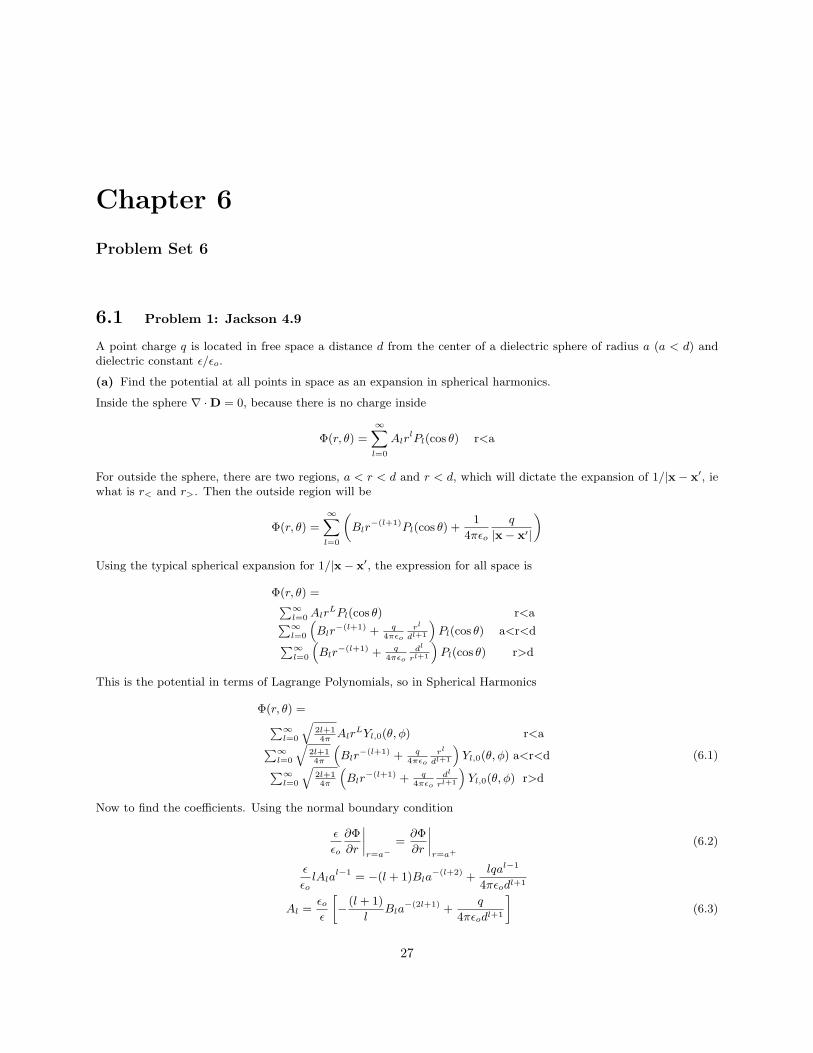
6.1 Problem 1: Jackson 4.9
A point charge q is located in free space a distance d from the center of a dielectric sphere of radius a (a < d) anddielectric constant ε/εo.
(a) Find the potential at all points in space as an expansion in spherical harmonics.
Inside the sphere ∇ ·D = 0, because there is no charge inside
Φ(r, θ) =
∞∑l=0
AlrlPl(cos θ) r<a
For outside the sphere, there are two regions, a < r < d and r < d, which will dictate the expansion of 1/|x− x′, iewhat is r< and r>. Then the outside region will be
Φ(r, θ) =
∞∑l=0
(Blr
−(l+1)Pl(cos θ) +1
4πεo
q
|x− x′|
)Using the typical spherical expansion for 1/|x− x′, the expression for all space is
Φ(r, θ) =∑∞l=0 Alr
LPl(cos θ) r<a∑∞l=0
(Blr
−(l+1) + q4πεo
rl
dl+1
)Pl(cos θ) a<r<d∑∞
l=0
(Blr
−(l+1) + q4πεo
dl
rl+1
)Pl(cos θ) r>d
This is the potential in terms of Lagrange Polynomials, so in Spherical Harmonics
Φ(r, θ) =∑∞l=0
√2l+14π
AlrLYl,0(θ, φ) r<a∑∞
l=0
√2l+14π
(Blr
−(l+1) + q4πεo
rl
dl+1
)Yl,0(θ, φ) a<r<d∑∞
l=0
√2l+14π
(Blr
−(l+1) + q4πεo
dl
rl+1
)Yl,0(θ, φ) r>d
(6.1)
Now to find the coefficients. Using the normal boundary condition
ε
εo
∂Φ
∂r
∣∣∣∣r=a−
=∂Φ
∂r
∣∣∣∣r=a+
(6.2)
ε
εolAla
l−1 = −(l + 1)Bla−(l+2) +
lqal−1
4πεodl+1
Al =εo
ε
[− (l + 1)
lBla
−(2l+1) +q
4πεodl+1
](6.3)
27

The other boundary condition is for tangential component
∂Φ
∂θ
∣∣∣∣r=a−
=∂Φ
∂θ
∣∣∣∣r=a+
Alal = Bla
−(l+1) +q
4πεo
al
dl+1(6.4)
Then the coefficients can easily be found from equation 3 and 4
Al =1
ε/εo + (l + 1)/l
(2l + 1
l
)q
4πεodl+1(6.5)
Bl =1
ε/εo + (l + 1)/l
(1− ε
εo
)qa2l+1
4πεodl+1(6.6)
Combining equations 5 and 6 into equation 1 yields the potential at every point in space. X
(b) Calculate the rectangular components of the electric field near the center of the sphere.
Expanding the potential inside the sphere
Φ(r, θ) = A1rP1(cos θ) + A2r2P2(cos θ) + . . .
From Quantum Mechanics, rP1(cos θ) = z and r2P2(cos θ) = z2 − x2 + y2, then the potential becomes
Φ(x, y, z) =q
4πεo
[3z
(ε/εo + 2)d2+
5(z2 − x2 − y2
)2(2ε/εo + 3)d3
+ . . .
]So then Ei = −
∫Φdxi. Then the component in Cartesian space
Ex =q
4πεod2
[5
2ε/εo + 3
x
d+ . . .
]Ey =
q
4πεod2
[5
2ε/εo + 3
y
d+ . . .
]Ez = − q
4πεod2
[3
ε/εo + 2+
5
2ε/εo + 3
z
d+ . . .
]X
(c) Verify that, in the limit ε/εo →∞, your result is the same as that for the conducting sphere.
Examining equation 2, the equation would blow-up if Al 6= 0, therefore Al = 0. This is the same for the conductor.Then from that and equation 4,
Bl = − q
4πεo
a2l+1
dl+1
which is the same as a conduction sphere. X
6.2 Problem 2: Jackson 4.10
Two concentric conducting spheres of inner and outer radii a and b , respectively, carry charges ±Q. The emptyspace between the spheres is half-filled by a hemispherical shell of dielectric (of dielectric constant ε/εo), as shown inthe figure.1
(a) Find the electric field everywhere between the spheres.
Let’s assume that E ∝ rr3 . Using Gauss’s Law for a sphere between the two spheres:∮
D · da = Q
2πr2 (εoE(r)− εE(r)) = Q
Q
2π(εo + ε)
r
r3= E(r)
Now checking the conditions on the solution. The curl of the electric field is obviously 0. The divergent of the fielddoes yield the charge density. By the uniqueness theorem, this is the correct solution. X
1Jackson. pg 174
28

(b) Calculate the surface-charge distribution of the inner sphere.
From Equation 4.40, in particular n · ((D2 −D1) = σfree. The half without the dielectric is
σfree = r ·D(a) = r · r
a2
Qεo
2π(εo + ε)=
Qεo
2πa2(εo + ε)
Now for part with the dielectric is directly
σfree =Qε
2πa2(εo + ε)X
(c) Calculate the polarization-charge density induced on the surface of the dielectric at r = a
The electric polarization is given by P = (ε− εo)E. Because in the free space ε = εo, the electric polarization for the
free space is P = 0. Therefore σpol = 0 for the free space half. Now, the polarization density is σpol = −n·(P1−P2).
For the dielectric part
σpol = −r ·P(a) = −rr
a2
(ε− εo)Q
2π(εo + ε)
σpol = − (ε− εo)Q
2πa2(εo + ε)X
6.3 Problem 3: Distressed Simple Cubic
Repeat the analysis of section 4.5 for a cubic crystal which is subjected to a stress such that the lattice separation iselongated along one edge of the cube (the x axis) and contracted along the other cube edges (the y and z axes) bythe amounts
ax = a(1 + δ) (6.7)
ay,z = a
(1− 1
2δ
)(6.8)
where a is the unstressed cubic lattice spacing. Find the susceptibility for two cases, considering that the molecularpolarizabilty γmol is a constant scalar (Hint: Calculate Enear at a particular dipole by considering only the 6 nearestdipoles in the cubic lattice):
(a) An electric field applied parallel to the x axis
The polarization is given on page 161 in Jackson as P = N〈pmol〉 and also 〈pmol〉 = εoγmol(E + Ei) From theprevious page Equation 4.63, Ei = P
3ε+ Enear. All that remains is to find Enear. From Equation 4.64:
Enear =3n(n · p)− p
r3(6.9)
29

Considering the six nearest neighbors, which occur from the shape(from class notes):
Ei =3n(npi)− pi
a3i
Ex =4px
a3x
− 2px
a3y
− 2px
a3z
Ey =4py
a3y
− 2py
a3x
− 2py
a3z
Ez =4pz
a3z
− 2pz
a3x
− 2pz
a3y
Now using the values for the expansion of the nearest neighbors and the fact that δ < 1 and the binomial expansion.
Ex =4px
a3(1 + δ)3− 2px
a3(1− 1
2δ)3 − 2px
a3(1− 1
2δ)3 =
4px
a3(1− 3δ)− 4px
a3
(1 +
3
2δ
)= −18pxδ
a3(6.10)
Ey =4py
a3(1− 1
2δ)3 − 2py
a3(1 + δ)3− 2py
a3(1− 1
2δ)3 =
2py
a3
(1 +
3
2δ
)− 2py
a3(1− 3δ) =
9pyδ
a3(6.11)
Ez =4pz
a3(1− 1
2δ)3 − 2pz
a3(1 + δ)3− 2pz
a3(1− 1
2δ)3 =
2pz
a3
(1 +
3
2δ
)− 2pz
a3(1− 3δ) =
9pzδ
a3(6.12)
So now Enear known. To simplify the problem, the fact that P = εoχE can be used. Since Ey = Ez = 0, thenPy = Pz = 0. So only Px is needed.
Px = Nγmol
(εoEx + εo
(−18
a3δ +
1
3εo
)Px
)→(
1 + Nγmol18
a3δεo −
Nγmol
3
)Px = NγmolεoEx(
1 + Nγmol18
a3δεo −
Nγmol
3
)χεoEx = NγmolεoEx → χ =
Nγmol
1− 13Nγmol + 18
a3 Nγmolδεo
X
(b) An electric field applied parallel to the y axis.
For an electric field in the y direction. As above, P = εoχE, then Ex = Ez = Px = Pz = 0. So only Enear for the ydirection is needed. Then
Py = Nγmol
(εoEy + εo
(9
a3δ +
1
3εo
)Py
)→(
1−Nγmol9
a3δεo −
Nγmol
3
)Py = NγmolεoEy(
1−Nγmol9
a3δεo −
Nγmol
3
)χεoEy = NγmolεoEy → χ =
Nγmol
1− 13Nγmol − 9
a3 Nγmolδεo
X
30

Chapter 7
Problem Set 7
7.1 Problem 1: Jackson 4.13
Two long, cylindrical conducting surfaces of radii a and b are lowered vertically into a liquid dielectric. If the liquidrises an average height h between the electrodes when a potential difference V is established between them, showthat the susceptibility of the liquid is
χe =
(b2 − a2
)ρgh ln(b/a)
εoV 2(7.1)
where ρ is the density of the liquid, g is the acceleration due to gravity, and the susceptibility of air is neglected.
The first thing to find is the electric field between the cylinders. There is no charge between the cylinders, so ∇2Φ = 0.From the symmetry of the problem, cylindrical coordinates are the proper choice, Further there is radial symmetry,so there is no polar coordinate. So the Laplacian is
1
r
∂
∂r
(r∂Φ
∂r
)= 0 (7.2)
The familiar solution is
Φ(r) = A ln (r/B)
Now the boundary condition that the difference of the two cylinders is V or more exact
Φ(b)− Φ(a) = A ln(b/a) = V ⇒ A =V
ln(b/a)
So the electric field is
E = −∂Φ
∂rr→ E =
−V
ln(b/a)
r
r
Now that the electric field is known, the electric displacement is simply D = εE for inside the liquid, and for abovethe liquid, the electric displacement is D = εoE. The work to raise the liquid is
W =1
2
∫E ·Dd3x =
1
2
∫ b
a
2πrdr
(∫ z
−d
εE2dz +
∫ l
z
εoE2dz
)where d is the length in the liquid and l is the length above. The work is then
W =1
2
∫ b
a
2πrdr
(∫ z
−d
εE2dz +
∫ l
z
εE2dz
)=
πV 2
ln(b/a)(ε (z + d) + εo (l − z))
From Equation 4.102, the force needed to left the liquid is
Fz =
(∂W
∂z
)V
=(ε− εo) πV 2
ln(b/a)
31

Now finding the volume of liquid that has been lifted is(b2 − a2
)πh. The mass is then m =
(b2 − a2
)ρπh. At
equilibrium, the force of gravity is equal to the force of the electric field.
(b2 − a2) ρπh =
(ε− εo) πV 2
ln(b/a)
(b2 − a2
)ρπh
εo=
(ε/εo − 1) πV 2
ln(b/a)
The susceptibility is defined as χe = ε/εo − 1. Then(b2 − a2
)ρπh
εo=
χeπV 2
ln(b/a)⇒ χe =
(b2 − a2
)ρgh ln(b/a)
εoV 2X
32

Chapter 8
Problem Set 8
8.1 Problem 1: Jackson 5.2
A long, right cylindrical, ideal solenoid of arbitrary cross section is created by stacking a large number of identicalcurrent-carrying loops one above the other, with N coils per unit length and each loop carrying a current I.
(a) In the approximation that the solenoidal coil is an ideal current sheet and infinitely long, use Problem 5.1 toestablish that any point outside the coil that H = 0, and that any point inside the coil the magnetic field isaxial and equal to
H = NI (8.1)
This can be solved using two ampere loops. Placing a loop outside the cylinder, it yields B = 0. Placing a secondloop through a side of the surface perpendicular to the bottom surface. So∮
B · dl = µoIenc
From the first loop that was outside the cylinder, the induced magnetic field outside is 0. This means that the onlyfield is inside the cylinder. The integral becomes∮
B · dl = µoIenc ⇒ BL = µoNIL
Using right hand rule, Bz = µoNI. In this system M = 0, then H = B/µo, therefore Bz = µoNI ⇒ H = NI. X
(b) For a realistic solenoid of circular cross section of radius a (Na 1), but still infinite in length, show that the“smoothed” magnetic field just outside the solenoid (averaged axially over several turns) is not zero, but is thesame in magnitude and direction as that of a single wire on the axis carrying a current I, even if Na → ∞.Compare fields inside and out.
In a real solenoid, it is not simple current loops stacked on each other. There is a little bind in the loop to connectthe loops. This means there is a current in the vertical direction. So what is the current? This can be found by thefact the total current moves up 1/N each loop. In each loop there is I/N in the vertical direction, so over a unitlength there is N loops, so the amount of vertical current is then NI/N = I. Therefore this current in the verticaldirection ∮
B · dl⇒ 2πρB = µoI ⇒ Bθ =µoI
2πρ
This is the same as a wire along the z-axis. As the number of loops increase per unit length, the more idealit will become. The size of inside is many orders of magnitude large than the field outside. To be more exact,µoNI/(µoI/2πρ) → 2πρN . So the field inside is 2πρN times larger. The directions of the two are perpendicular toeach other. X
33

8.2 Problem 2: Semi-Infinite Cylinder
Consider a semi-infinite solenoid, which we idealize as a cylindrical current sheet of radius a and azimuthal currentK per unit length, with one end at the origin and the other end at -∞ along the z-axis.
(a) Use the Biot-Savart Law to show that the magnetic induction on the axis is
Bz =µoK
2
[1− z
(a2 + z2)1/2
](8.2)
Let’s begin by thinking of a single current loop at the origin. The magnetic-flux density is
Bz =µoI
4π
∮dl× x
|x|3
Because this has to end the z direction, x = a cos φρ + a sin φφ + zz, |x|3 =(a2 + z2
)3/2, and dl = −a sin φρ +
a cos φφ + 0z. Then
Bz =µoI
4π
1
(a2 + z2)3/2
∫ 2π
0
[−az cos φ + az sin φ + a2] dφ
=µoI
2
a2
(a2 + z2)3/2z
Now this has to be integrated from start to finish of the cylinder remembering that I → K
Bz =µoa
2K
2z
∫ 0
−∞
dz
(a2 + z2)3/2
=µoa
2K
2z
z
(a2 + z2)1/2
∣∣∣∣0−∞
=µoK
2z cos θ
∣∣∣∣πθ1
where θ is the angle that the origin makes with the edge at the end of the cylinder and cos θ = z
(a2+z2)3/2 , then
Bz =µoK
2
[1− z
(a2 + z2)3/2
]X
(b) Use a Taylor series expansion of the field near the axis together with ∇ ·B = 0 and ∇×B = 0 to show that themagnetic induction near the axis is
Bρ ≈µoK
4
a2ρ
(a2 + z2)3/2(8.3)
Bz ≈µoK
2
[1− z
(a2 + z2)1/2− 3
4
a2zρ2
(a2 + z2)5/2
](8.4)
The two conditions, ∇·B and ∇×B, lead to Laplace’s Equation ∇2Φmag = 0 and B = −∇Φmag. From electrostatics,Φmag = R(ρ)Z(z)Q(θ). The radial solutions are the Bessel and Neumann functions. Then
Φmag = (AJν(kρ) + BNν(kρ)) Ce−kzDeiνθ
From symmetry, ν = 0 and as ρ → 0 has to be well define B = 0. Then Φmag = CJ0(kρ)e−kz. Then the inducedfield is
B = −∇Φmag = −[ρ
∂
∂ρ+ z
∂
∂z
]Φmag
= −Ck∂Jo(x)
∂xe−kxρ + CkJo(kρ)e−kz z
34

From Arfken’s book, ∂Jo(x)∂x
= −J1(x)1. Expanding the two terms2,
Bρ = CkJ1(kρ)e−kz ≈ Cke−kz
(kρ
2− k3ρ3
16
)Bz = CkJ0(kρ)e−kz ≈ Cke−kz
(1− k2ρ2
4
)Now, Bz(0, z) = Cke−kz, this has to be the case, because it has to be continuous. It follows that ∂nBz(0,z)
∂zn =
(−1)n Ckn+1e−kz. With this substitution,
Bρ ≈ Cke−kz
(kρ
2
)≈ ρ
2
∂Bz(0, z)
∂z
Bz ≈ Cke−kz
(1− k2ρ2
4
)≈ Bz(0, z)− ρ2
4
∂2Bz(0, z)
∂z
Using Bz from part one finally
Bρ ≈ρ
2
∂
∂z
µoK
2
[1−
z
(a2 + z2)3/2
]⇒ Bρ ≈
µoK
4
a2ρ
(a2 + z2)3/2
Bz ≈µoK
2
[1−
z
(a2 + z2)3/2
]−
ρ2
4
∂2
∂z
[µoK
2
[1−
z
(a2 + z2)3/2
]]
Bz ≈µoK
2
[1−
z
(a2 + z2)1/2−
3
4
a2zρ2
(a2 + z2)5/2
]X
8.3 Problem 3: Jackson 5.6
A cylindrical conductor of radius a has a hole of radius b bored parallel to, and centered a distance d from, thecylinder axis (d + b < a). The current density is uniform throughout the remaining metal of the cylinder and isparallel to the axis. Use Ampere’s law and principle of linear superposition to find the magnitude and the directionof the magnetic-flux density in the hole.
From the hint to use superposition, we will first find the magnetic-flux density for the cylindrical conductors. For theone with radius a applying Ampere’s law in the form of Equation 5.24∮
C
B · dl = µo
∫S
J · nda
B2πr2 = µoJπr2 → B =µo
2Jrz × r
Now for the hole, it has to be the same except that it has a different coordinate system, that is related by a lineartransformation, directly B′ = µo
2J ′r′z × r′, because this is a hole the current density is in the opposite direction,
J ′ = −J . Next is relating rr to r′r′. Defining the center of the hole on the −y-axis of the cylinder, the relationshipis r′r′ = rr + dy. Now linear superposition can be used to find
Bfinal = B + B′ =µo
2Jz × (rr − rr − dy)
=µo
2Jdz × (−y) ⇒ Bfinal =
µoJd
2x X
8.4 Problem 4: Jackson 5.13
A sphere of radius a carries a uniform surface-charge distribution σ. The sphere is rotated about a diameter withconstant angular velocity ω. Find the vector potential and magnetic-flux density both inside and outside the sphere.
1Arfken. MMP 5thed. pg.6732Arfken. MMP 5thed. pg.670
35

The surface current is ~J = σ~v = σ(~ω × ~r′) = σaω sin θ′(r′ − a)φ′. The surface current is then related to l = 1 andm = 1 only, because of the sine term. The
36

vector potential is then
Aφ(r, θ) =µo
4π
∑l
P 1l (cos θ)
l(l + 1)
∫σωaδ(r′ − a)
rl<
rl+1>
P 1l (cos θ′)r′2 sin2 θ′dr′dθ′dφ
= −µo
2
∑l
P 1l (cos θ)
l(l + 1)
σωa3rl<
rl+1>
∫ π
0
P 1l (cos θ′)P 1
1 (cos θ) sin θ′dθ′
= −µoσωa3
4
r<
r2>
P 11 (cos θ)
4
3
=µoσωa3r<
3r2>
sin θ
Now for the magnetic field, B = ∇×A. This needs to be done for the interior (a > r) and exterior (a < r). The vector
potential interior is Aint =1
3µoσωar sin θφ . The vector potential for exterior is Aext(r, θ) =
1
3µoσωa4 sin θ
r2φ So
for the interior
Bint(r, θ) = r1
r sin θ
∂
∂θ
(µoσωa
3sin2 θ
)− θ
1
r
∂
∂r
(µoσωar2 sin θ
3
)Bint(r, θ) =
2
3µoσωa
[cos θr − sin θθ
]Now for the exterior
Bext(r, θ) = r1
r sin θ
∂
∂θ
(µoσωa4
3r2sin2 θ
)− θ
1
r
∂
∂r
(µoσωa4 sin θ
3
1
r
)
Bext(r, θ) =1
3
µoσωa4
r3
[2 cos θr + sin θθ
]X
37

38

Chapter 9
Problem Set 9
9.1 Problem 1: Jackson 5.17
A current distribution J(x) exists in a medium of unit relative permeability adjacent to a semi-infinite slab of materialhaving relative permeability µr and filling the half space, z < 0.
(a) Show that for z > 0 the magnetic induction ca be calculated by replacing the medium of permeability µr by animage current distribution, J∗, with components,
(µr − 1
µr + 1
)Jx(x, y,−z),
(µr − 1
µr + 1
)Jy(x, y,−z), −
(µr − 1
µr + 1
)Jz(x, y,−z) (9.1)
The field z > 0 is
B =µo
4π
∫(J + J∗)× (x− x′)
|x− x′|3 d3x′ (9.2)
The field z < 0 is
B =µo
4π
∫J× (x− x′)
|x− x′|3 d3x′ (9.3)
At the boundary of z = 0, the normal component of the field must be continuous, so above
Bz+ (−z) =µo
4π
∫ (Jx + J∗x+ )(y − y′)− (Jy + J∗
y+ )(x− x′)((x− x′)2 + (y − y′)2 + z′2
)3/2d3x′
below
Bz−(z) =µo
4π
∫J∗x−(y − y′)− J∗y−(x− x′)(
(x− x′)2 + (y − y′)2 + z′2)3/2
d3x′
Then Bz+(−z) = Bz−(z). Therefore
Jx(−z) + J∗x+(z) = J∗x−(z) (9.4)
Jy(−z) + J∗y+(z) = J∗y−(z) (9.5)
Now for the tangential components of the magnetic field must be continuous, and H = B/µ. So for above
Hx+(−z) =1
4π
∫ −z′(Jy + J∗y+)− (y − y′)(Jz + J∗z+)
((x− x′)2 + (y − y′)2 + z′2)3/2d3x′
Hy+(−z) =1
4π
∫(x− x′)(Jz + J∗z+) + z′(Jx + J∗x+)
((x− x′)2 + (y − y′)2 + z′2)3/2d3x′
Below
Hx−(z) =1
4πµr
∫ −z′(J∗y−)− (y − y′)(J∗z−)
((x− x′)2 + (y − y′)2 + z′2)3/2d3x′
Hy−(z) =1
4πµr
∫(x− x′)(J∗z−) + z′(J∗x−)
((x− x′)2 + (y − y′)2 + z′2)3/2d3x′
39

From H+ = H−
µrJz(−z) + µrJz+(z) = Jz−(z) (9.6)
µrJy(−z)− µrJy+(z) = Jy−(z) (9.7)
µrJx(−z)− µrJx+(z) = Jx−(z) (9.8)
From eq 4 and 7, and eq 5 and 8
Jx+ (z) =µr − 1
µr + 1Jx(−z) Jx− (z) =
2µr
µr + 1Jx(z) (9.9)
Jy+ (z) =µr − 1
µr + 1Jy(−z) Jy− (z) =
2µr
µr + 1Jy(z) (9.10)
Now for the z components.
∇ · J∗− = 0 =∂J∗x−
∂x+
∂J∗y−
∂y+
∂J∗z−
∂z=
2µr
µr + 1
(∂Jx
∂x+
∂Jy
∂y
)+ µr
∂
∂z(Jz + Jz+) = − 2µr
µr + 1
∂Jz
∂z+ µr
∂
∂z(Jz + Jz+)
Then solving and integrating
−µr − 1
µr + 1
∫∂Jz =
∫∂Jz+ ⇒ −
µr − 1
µr + 1Jz(−z) = Jz+ (z) (9.11)
From equations 9, 10, 11 for J∗+ matches equation 1. X
(b) Show that for z < 0 the magnetic induction appears to be due to a current distribution [2µr/(µr + 1)]J in amedium of unit relative permeability.
Combining equation 6 with equation 11 to find
J∗z−(z) =2µr
µr + 1Jz (z) (9.12)
Adding equation 12 with the J− parts of equations 9, 10 to find that J∗− = [2µr/(µr + 1)]J X
9.2 Problem 2: Jackson 5.19
A magnetically “hard” material is in the shape of a right circular cylinder of length L and radius a. The cylinder hasa permanent magnetization Mo, uniform throughout its volume and parallel to its axis.
(a) Determine the magnetic field H and magnetic induction B at all points on the axis of cylinder, both inside andoutside.
Because there is no free current, this is a magnetostatic potential problem. This problem then can be treated as anelectrostatic problem. Because the magnetization is uniform, ρM = −∇ ·M = 0. The surface ‘charge’ density is thenσM = n ·M = ±Mo at the caps. The potential is then
ΦM =1
4π
∫σM
|x− x′|d3x′
This is evaluated at the caps only. Then
Φ1 =Mo
4π
ρ∫0
2πρdρ√ρ2 + (z − L/2)2
=Mo
2
[√ρ2 + (z − L/2)2
]a
0
=Mo
2
(√a2 + (z − L/2)2 −
√(z − L/2)2
)This can easily be show for the bottom with symmetry that
Φ2 = −Mo
2
(√a2 + (z + L/2)2 −
√(z + L/2)2
)
40

The potential over all space is Φ = Φ1 + Φ2.
Φ =Mo
2
√√√√a2 +
(z −
L
2
)2−
√√√√a2 +
(z +
L
2
)2−∣∣∣∣z − L
2
∣∣∣∣ + ∣∣∣∣z +L
2
∣∣∣∣
The magnetic field has two cases, one inside
Hz =∂Φ
∂z
Hz =Mo
2
z + L/2√a2 + (z + L/2)2
−z − L/2√
a2 + (z − L/2)2− 2
And outside
Hz =Mo
2
z + L/2√a2 + (z + L/2)2
−z − L/2√
a2 + (z − L/2)2
Now the induced field is Bz = µo(Hz + M). In this case, M = Mo inside and M = 0 outside. Then the induced fieldboth inside and outside is
Bz =µoMo
2
z + L/2√a2 + (z + L/2)2
−z − L/2√
a2 + (z − L/2)2
X
(b) Plot the ratios B/µoMo and H/Mo on the axis as functions of z for L/a = 5.
See last page
9.3 Problem 3: Jackson 5.22
Show that in general a long, straight bar of uniform cross-sectional area A with uniform lengthwise magnetization M ,when placed with its flat end against as infinitely permeable flat surface, adheres with a force given approximatelyby
F ' µo
2AM2 (9.13)
Relate your discussion to the electrostatic considerations in Section 1.11.
So consider this as two long straight bars with uniform cross-sectional areas A with uniform magnetization, M . Onerod runs from z = 0 to z = −L and the other from z = 0 to z = L. These two dipoles are “head” to “tail”, sothe components of the B-field cancel everywhere except at z = 0. Now, let’s introduce a small separation zo. Thepotential energy on the real rod from the image rod is
W (zo) = −∫
M ·Bid3x = −M
∫V
Bz,id3x
Because the image rod is not moved and the rod is much longer than it is any other direction
W (zo) = −M
∫V
Bz,id3x ≈ −MA
∫ zo+L
zo
Bz,i(z)dz
The force from the change in the vertical separation
Fz = −dW (zo)
dzo
∣∣∣∣zo=0
= MA(Bz,i(L)−Bz,i(0))
From the previous problem, if the shape is circular, which is not that bad of an approximation, the induced field is
Bz,i(z) =µoM
2
(z + L√
a2 + (z + L)2− z√
a2 + z2
)
41

Figure 9.1: H/Mo = 12
(z/L+1/2√
1/25+(z/L+1/2)2− z/L−1/2√
1/25+(z/L−1/2)2
)-0 |z/L| > 1/2 or1 |z/L| ≤ 1/2
The force becomes
Fz =µoM
2A
2
(2L√
a2 + 4L2− L√
a2 + L2− L√
a2 + L2+ 0
)
Now the condition that a L, Fz = −µoM2A
2X
Now comparing the problem with 1.11. From the previous problem inside the rod, σM = M on the end above theplain, and σM = −M below the plain. So
Bz =
µoM inside
0 outside
Because of the constant induced field, this is similar to a constant electric field. In fact, the magnetic potential issimilar to the electric potential of plane capacitors with σE/εo → µoσM . To create a capacitor, lets separate the realrod, which is the one above the plane, and the image rod. Now on page 43, F/A = σ2/2εo for a capacitor. Then
F/A = σ2Mµ2
o/2µo → F/A = µoσ2M/2. Finally the value of σM , F/A = µoM
2/2 → F =µo
2AM2
42

Figure 9.2: B/µoMo = 12
(z/L+1/2√
1/25+(z/L+1/2)2− z/L−1/2√
1/25+(z/L−1/2)2
)
43

44

Chapter 10
Problem Set 10
10.1 Problem 1: Jackson 5.14
A long, hollow, right circular cylinder of inner (outer) radius a (b), and of relative permeability µr, is placed in aregion of initially uniform magnetic-flux density Bo at right angles to the field. Find the flux density at all pointsin space, and sketch the logarithm of the ratio of the magnitudes of B on the cylinder axis to Bo as a function oflog10 µr for a2/b2 = 0.5, 0.1. Neglect end effects.
Because there are no end effects, this problem can be reduced to a two dimensional problem. With the z-axis thelength of the cylinder and the Bo in the x-direction. With those being set, this is much like the problem donein class. So ∇ · B = ∇ · (µH) = 0 and for inside and outside ∇ × H = 0. The solution is H = −∇Φm where
Φ = ao + bo ln ρ +∞∑
n=1
anρn (cos nϕ + sin nϕ) +∞∑
n=1
bnρ−n (cos nϕ + sin nϕ). All that remains is to solve for the
coefficients. By symmetry the sine terms can be dropped. For ρ > b, an = 0, and for ρ < a, bn = 0. So the potentialis
Φm(ρ, ϕ) =
∑∞n=1 αnρn cos nϕ ρ < a∑∞n=1
(βnρn cos nϕ + γnρ−n cos nϕ
)a < ρ < b∑∞
n=1 δnρ−n cos nϕ ρ > b
H has to be continuous at the boundaries. At ρ = b, the differential with respect to the radial is
Bo
µocos ϕ +
∞∑n=1
nb−(n+1)δn cos nϕ = µr
∞∑n=1
−n(βnbn−1 − γnb−(n+1)
)cos nϕ
From this n = 1, so
Bo
µo+ δ1b
−2 = −µrβ1 + µrγ1b−2 (10.1)
The tangential continuation at ρ = b
−Bo
µo+ δ1b
−2 = β1 + γ1b−2 (10.2)
Likewise at ρ = a
α1 = µrβ1 − µrγ1a−2 (10.3)
α1 = β1 + γ1a−2 (10.4)
Reducing the number of coefficients in equations 1 and 2
β1 =(µr − 1)
2µrδ1b
−2 − (µr + 1)
2µr
Bo
µo(10.5)
γ1 =(µr + 1)
2µrδ1 +
(1− µr)
2µr
Bo
µob2 (10.6)
45
Doing the same with equations 3 and 4
β1 =(µr + 1)
2µrα1 (10.7)
γ1 =(µr − 1)
2µrα1a
2 (10.8)
Now combining equations 5 and 7
α1 =(µr − 1)
(µr + 1)δ1b
−2 − Bo
µo(10.9)
Now for equations 6 and 8
α1 =(µr + 1)
(µr − 1)δ1a
−2 − b2
a2
Bo
µo(10.10)
Equating 9 and 10
δ1 =
(1− a2
b2
) (µ2
r − 1)b2
(µr + 1)2 b2 − (µr − 1)2 a2
Bo
µob2 (10.11)
With equation 9 and 11
α1 =−4µrb
2
(µr + 1)2 b2 − (µr − 1)2 a2
Bo
µo(10.12)
Placing equation 12 into equation 7 and also equation 8
β1 =−2 (µr + 1) b2
(µr + 1)2 b2 − (µr − 1)2 a2
Bo
µo(10.13)
γ1 =−2 (µr − 1) b2
(µr + 1)2 b2 − (µr − 1)2 a2
Bo
µoa2 (10.14)
Now the field is
H =
−α1 cos ϕρ + α1 sin ϕϕ ρ < a
−(β1 − γ1
ρ2
)cos ϕρ +
(β1 + γ1
ρ2
)sin ϕϕ a < ρ < b(
Boµo
+ δ1ρ2
)cos ϕρ−
(Boµo
+ δ1ρ2
)sin ϕϕ ρ > b
See last page for graph X
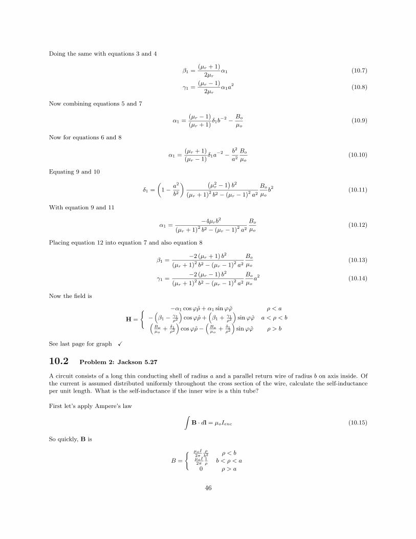
10.2 Problem 2: Jackson 5.27
A circuit consists of a long thin conducting shell of radius a and a parallel return wire of radius b on axis inside. Ofthe current is assumed distributed uniformly throughout the cross section of the wire, calculate the self-inductanceper unit length. What is the self-inductance if the inner wire is a thin tube?
First let’s apply Ampere’s law ∫B · dl = µoIenc (10.15)
So quickly, B is
B =
µoI2π
ρb2
ρ < bµoI2π
1ρ
b < ρ < a
0 ρ > a
46

The energy of the magnetic field per length of the system is given by Eq. 5.148
W =1
2
∫H ·Bd3x =
1
2µo
∫B2d3x
=2π
2µo
(µoI
2π
)2(∫ b
0
ρ3dρ
b4+
∫ a
b
dρ
ρ
)=
π
µo
(µoI
2π
)2(1
4+ ln
(a
b
))=
µoI2
16π
(4 ln
(a
b
)+ 1)
From Eq. 5.152, W = 12LI2. The self-inductance per unit length is
1
2LI2 =
µoI2
16π
(4 ln
(a
b
)+ 1)⇒ L =
µoI2
8π
(4 ln
(a
b
)+ 1)
X
Now if the inner wire is a tube B = 0 for ρ < b, so there is only the middle term which yields a self-inductance perunit length of
L =µo
2πln(a
b
)X
10.3 Problem 3: Jackson 5.29
The figure (See Jackson pg. 232) represents a transmission line consisting of two, parallel perfect conductors ofarbitrary, but constant, cross section. Current flows down one conductor and returns via the other.Show that the product of the inductance per unit length L and the capacitance per unit length C is
LC = µε (10.16)
where µ and ε are the permeability and the permittivity of the medium surrounding the conductors.
First using Ampere’s Law for outside the wires∫B · dl = µI ⇒ B =
µI
2πρ
But inside the wire B = 0. The vector potential is
Az =
∫Bφdρ =
∫µI
2πρdρ ⇒ Az = −µI
2πln
(ρ
ρo
)where ρo = a, b. The work per unit length can be found from Eq. 5.149
W =1
2
∫J ·Ad3x =
1
2
∫(JaAdaa + JbAdab)
=1
2
µI
2π
(∫ a
0
2πI
πa2ln
(d
b
)ρadρa +
∫ b
0
2πI
πb2ln
(d
a
)ρbdρb
)=
1
2
µI
2π
(a2πI
πa2ln
(d
b
)+
b2πI
πb2ln
(d
a
))=
µI2
4πln
(d2
ab
)Relating this to the self-inductance per unit length
1
2LI2 =
µI2
4πln
(d2
ab
)⇒ L =
µ
2πln
(d2
ab
)From the second problem 1.7, the capacitance is
C =2πε
ln(
d2
ab
) (10.17)
47

Then
LC =µ
2πln
(d2
ab
)2πε
ln(
d2
ab
) ⇒ LC = µε X
Capacitance The electric field for a wire is given by
~E =Q
2πεo
r
r
The potential between the two wire is
Φ =
∫~E · d~l =
Q
2πεo
[∫ d−a2
a1
dr
r+
∫ d−a1
a2
dr
r
]=
Q
2πεo
[ln
(d− a2
a1
)+ ln
(d− a1
a2
)]=
Q
2πεo
[ln
((d− a2) (d− a1)
a1a2
)]The capacitance is given by C = Q
Φ. Then
C =Q
Φ=
Q
Q2πεo
[ln(
(d−a2)(d−a1)a1a2
)]=
2πεo
ln(
(d−a2)(d−a1)a1a2
)Since the distance between the wires is much large than their radii, d−a1 ≈ d−a2 ≈ d. Then capacitance reduces to
C ≈ 2πεo
ln(
d2
a1a2
)
48

Figure 10.1: BBo
= µr
(µr+1)2−(µr−1)2 a2
b2
49

50

Chapter 11
Problem Set 11
11.1 Problem 1: Jackson 6.8
A dielectric sphere of dielectric constant ε and radius a is located at the origin. There is a uniform applied electricfield Eo in the x direction. The sphere rotates with an angular velocity ω about the a axis. Show that there is amagnetic field H = −∇ΦM , where
ΦM =3
5
(ε− εo
ε + 2εo
)εoEoω
(a
r>
)5
· xy (11.1)
where r> is the larger of r and a. The motion is nonrelativistic.
First the polarization from Eq. 4.57
Px = 3ε− εo
ε + 2εoEox → Px = αEox (11.2)
So the volume charge density is −∇ ·P = 0. The surface charge density is
σ = n ·M = n · ((r ·P)ωz) = αεoEoωa sin θ cos θ cos φ
= −αεoEoωa
√8π
15
1
2[Y2,1 − Y2,−1]
The potential is
ΦM =1
4π
∫σ′da′
|x− x′|
= −αεoEoωa
√8π
15
1
2
a2
4π
∑ 4π
2l + 1
rl<
rl+1>
Ylm(θ, φ)×∫Y ∗
lm(θ′, φ′)[Y2,1(θ
′, φ′)− Y2,−1(θ′, φ′)
]sin θ′dθ′dφ′
= −αεoEoωa
√8π
15
1
2
a2
5
r2<
r3>
[Y2,1(θ, φ)− Y2,−1(θ, φ)]
= −αεoEoωa
√8π
15
1
2
a2
5
r2<
r3>
[−2
√15
8πsin θ cos θ cos φ
]
=3
5
ε− εo
ε + 2εoεoEoωa3 r3
<
r5>
sin θ cos θ cos φ
ΦM =3
5
ε− εo
ε + 2εoεoEoωxz
(a
r>
)5
X
51

11.2 Problem 2: Jackson 6.20
An example of the preservation of causality and finite speed of propagation in spite of the use of the Coulomb gaugeis afforded by a dipole source that is flashed on and off at t = 0. The effective charge and current densities are
ρ(x, t) = δ(x)δ(y)δ′(z)δ(t) (11.3)
Jz(x, t) = −δ(x)δ(y)δ(z)δ′(t) (11.4)
where the prime means differentiation with respect to the argument. This dipole is of unit strength and it points inthe negative Z direction.
(a) Show that the instantaneous Coulomb potential (6.23) is
Φ(x, t) = − 1
4πεoδ(t)
z
r3(11.5)
Using Eq. 6.23
Φ(x, t) =1
4πεo
∫ ρ
|x − x′|d3
x =1
4πεo
∫δ(x
′)δ(y′)δ
′(z′)δ(t)
d3x
|x − x′|= −
1
4πεoδ(t)
(∂
∂z′1
|z − z′|
)= −
1
4πεoδ(t)
(−
−z′ − z
|x − z′|3
)= −
1
4πεoδ(t)
z
r3X
(b) Show that the transverse current Jt with a factor of 2/3 multiplying the delta function coming from treatingthe gradient of z/r3 according to (4.20).
Jt(x, t) = −δ′(t)
[2
3ε3δ(x)− ε3
4πr3+
3
4πr3n(ε3 · n)
](11.6)
From Eq. 6.25 and 6.29
Jt = J− Jl = J− 1
µoc2∇∂Φ
∂t= −δ(x)δ(y)δ(z)δ′(t)z +
1
4π∇(δ′(t)
z
r3
)= −δ(x)δ(y)δ(z)δ′(t)z +
1
4πδ′(t)
(4π
3δ(x)δ(y)δ(z)z − 3r(z · r)− z
r3
)= −δ′(t)
(2
3δ(x)z − 1
4πr3z +
3
4πr3r(z · r)
)X
(c) Show that the electric and magnetic fields are causal and that the electric field components are (with Ey thesame as Ex except with cos φ replaced by sin φ),
Ex(x, t) =1
4πεo
c
r
[−δ′′(r − ct) +
3
rδ′(r − ct)− 3
r2δ(r − ct)
]sin θ cos θ cos φ (11.7)
Ez(x, t) =1
4πεo
c
r
[sin2 θδ′′(r − ct) + (3 cos2 θ − 1) ·
(δ′(r − ct)
r− δ(r − ct)
r2
)](11.8)
From section 6.3, A is causal, ∴ B is causal. Now for E. From equation 6.48
A =µo
4π
∫1
R[J]ret d3x
∂A
∂t= −µo
4π
∫1
R
∂
∂t
[δ′(
t− R
c
)(δ(x′)z +
1
4π∇′ ∂
∂z′1
r′
)]d3x′
= −µo
4π
1
rδ′′(
t− R
c
)− µo
4π
∫dk
2π
1
R
∂2
∂t2eik(t−R/c) 1
4π∇′ ∂
∂z′1
r′d3x′
Now
∇′2 eik(t−R/c)
R=
1
R(−ik/c)2eik(t−R/c) − eik(t−R/c)4πδ(x− x′)
=1
c2
∂2
∂t2eik(t−R/c)
R− eikt4πδ(x− x′)
52
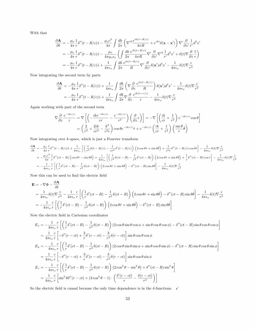
With that
∂A
∂t= −µo
4π
1
rδ′′(t−R/c)z − µoc
2
4π
∫dk
2π
(∇′2 eik(t−R/c)
4πR+ eiktδ(x− x′)
)∇′ ∂
∂z′1
r′d3x′
= −µo
4π
1
rδ′′(t−R/c)z − µo
4πµoεo
(∫dk
2π
eik(t−R/c)
4πR∇′ ∂
∂z′∇′2 1
r′d3x′ + δ(t)∇ ∂
∂z
1
r
)= −µo
4π
1
rδ′′(t−R/c)z +
1
4πεo
∫dk
2π
eik(t−R/c)
R∇′ ∂
∂z′δ(x′)d3x′ − 1
4πεoδ(t)∇ z
r3
Now integrating the second term by parts
∂A
∂t= −µo
4π
1
rδ′′(t−R/c)z +
1
4πεo
∫dk
2π
(∇ ∂
∂z
eik(t−R/c)
R
)δ(x′)d3x′ − 1
4πεoδ(t)∇ z
r3
= −µo
4π
1
rδ′′(t−R/c)z +
1
4πεo
∫dk
2π∇ ∂
∂z
eik(t−r/c)
r− 1
4πεoδ(t)∇ z
r3
Again working with part of the second term
∇ ∂
∂z
e−ikr/c
r= ∇
[(− ike−ikr/c
cr− e−ikr/c
r2
)(∂
∂zr
)]= −∇
[(ik
cr+
1
r2
)e−ikr/c cos θ
]=
(2
r3+
2ik
cr2− k2
c2r
)cos θe−ikr/cr + e−ikr/c
(ik
cr+
1
r2
)(sin θ
rθ
)Now integrating over k-space, which is just a Fourrier transform
∂A
∂t= −
µo
4π
1
rδ′′(t− R/c)z +
1
4πεo
[(1
r3δ(t− R/c)−
1
cr2δ′(t− R/c)
)(2 cos θr + sin θθ
)+
1
c2rδ′′(t− R/c) cos θr
]−
1
4πεo
δ(t)∇z
r3
= −µoc3
4π
1
rδ′′(ct− R)
(cos θr − sin θθ
)+
c
4πεo
[(1
r3δ(ct− R)−
1
r2δ′(ct− R)
)(2 cos θr + sin θθ
)+
1
rδ′′(ct− R) cos r
]−
1
4πεo
δ(t)∇z
r3
= −1
4πεo
c
r
[(1
rδ′(ct− R)−
1
r2δ(ct− R)
)(2 cos θr + sin θθ
)− δ
′′(ct− R) sin θθ
]−
1
4πεo
δ(t)∇z
r3
Now this can be used to find the electric field
E = −∇Φ− ∂A
∂t
=1
4πεoδ(t)∇ z
r3− 1
4πεo
c
r
[(1
rδ′(ct−R)− 1
r2δ(ct−R)
)(2 cos θr + sin θθ
)− δ′′(ct−R) sin θθ
]− 1
4πεoδ(t)∇ z
r3
= − 1
4πεo
c
r
[(1
rδ′(ct−R)− 1
r2δ(ct−R)
)(2 cos θr + sin θθ
)− δ′′(ct−R) sin θθ
]Now the electric field in Cartesian coordinates
Ex = − 1
4πεo
c
r
[(1
rδ′(ct−R)− 1
r2δ(ct−R)
)(2 cos θ sin θ cos φ + sin θ cos θ cos φ)− δ′′(ct−R) sin θ cos θ cos φ
]=
1
4πεo
c
r
[−δ′′(r − ct) +
3
rδ′(r − ct)− 3
r2δ(r − ct)
]sin θ cos θ cos φ
Ey = − 1
4πεo
c
r
[(1
rδ′(ct−R)− 1
r2δ(ct−R)
)(2 cos θ sin θ sin φ + sin θ cos θ sin φ)− δ′′(ct−R) sin θ cos θ sin φ
]=
1
4πεo
c
r
[−δ′′(r − ct) +
3
rδ′(r − ct)− 3
r2δ(r − ct)
]sin θ cos θ sin φ
Ez = − 1
4πεo
c
r
[(1
rδ′(ct−R)− 1
r2δ(ct−R)
)(2 cos2 θ − sin2 θ
)+ δ′′(ct−R) sin2 θ
]=
1
4πεo
c
r
[sin2 θδ′′(r − ct) + (3 cos2 θ − 1) ·
(δ′(r − ct)
r− δ(r − ct)
r2
)]So the electric field is causal because the only time dependence is in the δ-functions. X
53

11.3 Problem 3: Jackson 6.11
A transverse plane wave is incident normally in vacuum on a perfectly absorbing flat screen.
(a) From the law of conservation of linear momentum, show that the pressure (called radiation pressure) exerted onthe screen is equal to the field energy per unit volume in the wave.
The total electromagnetic momentum in an infinitesimal volume for a small area, ∆A over a small time, ∆t,
∆P = g∆Ac∆t
The force due to the momentum, F = ∆P/∆t = g∆Ac. The pressure is then perpendicular to the force per area.
p =g∆Ac
∆A= gc =
S
c= energy per unit volume or u X
(b) In the neighborhood of the earth the flux of electromagnetic energy from the sun is approximately 1.4 W/m2.If an interplanetary “sailplane” had a sail of mass 1 g/m2 of area and negligible other weight, what would beits maximum acceleration in meters per second squared due to the solar radiation pressure? How does thiscompare with the acceleration due to the solar “wind” (corpuscular radiation)?
The acceleration do the radiation pressure
arad =S/c
m/A=
1.4× 10³/(3× 108)
10−6⇒ arad ≈ 4.67× 10⁻³ m/s2
There are 105 protons/m2s with an average velocity v = 4× 10⁵ m/s
awind =mv/tA
m/A=
1.67× 10−27 × 4× 105 × 105
10−6= 6.68× 10
−14m/s
2
So arad awind X
54

Chapter 12
Problem Set 12
12.1 Problem 1: Jackson 6.4
A uniformly magnetized and conducting sphere of radius R and total magnetic moment m = 4πMR3/3 rotates aboutits magnetization axis with angular speed ω. In the steady state no current flows in the conductor. The motion isnonrelativistic; the sphere has no excess charge on it.
(a) By considering Ohm’s law in the moving conductor, show that the motion induces an electric field and a uniformvolume charge density in the conductor, ρ = −mω/πc2R3.
Here there are no free currents, so there is scalar potential that can describe the magnetic field. H = B/µo −M →∇ ·H = −∇ ·M, then ∇2ΦM = ∇ ·M. Here M = Mη (R− r) z1, so
∇ ·M =∂
∂zMη(R− r) = −Mδ(r −R)
∂r
∂z
= −Mδ(r −R)z
r= −Mδ(r −R) cos θ
Then
∇2ΦM = −Mδ(r − R) cos θ ⇒ Φ =
1
4π
∫Mδ(r − R) cos θ′
|r− r′|d3r′
This integral can be solved using a multipole expansion as done with electrostatics for inside a sphere.
ΦM =1
4π
∞∑l=0
∑m
4π
2l + 1
∫ Mδ(r′ − R) cos θ′
r′l+1Y∗
lm(θ′, ϕ
′)d3
r′r
lYlm(θ, ϕ)
=1
4π
∞∑l=0
l∑m=−l
4π
2l + 1
√4π
3M
R2
Rl+1
∫Y10Y
∗lmdΩr
lYlm
=1
4π
∞∑l=0
l∑m=−l
4π
2l + 1
√4π
3Mδl,1δm,0r
lYlm =
1
3Mr cos θ =
1
3Mz
The magnetic field inside the sphere is H = −∇ · Φ = 13Mz. The magnetic induction is
B = µo (H + M) = µo
(1
3Mz +
1
3Mz
)⇒ B =
2
3µoMz
From Ohm’s Law
E = −v × B = − (ω × r) × B =2
3µoMωz × (z × r) =
2
3µoMω (z · rz − r)
E = −2
3µoMω (xx + yy) = −
1
2
µomω
R3(xx + yy)
The charge density is
∇ ·E =ρ
εo= −4
3µoMω = −4
3
Mω
εoc2= − mω
πεoπc2R3
∇ ·E =ρ
εo= − mω
πεoπc2R3⇒ ρ = − mω
ππc2R3X
1Here η is a step function
55

(b) Because the sphere is electrically neutral, there is no monopole electric field outside. Use symmetry argumentsto show that only a quadrupole field exists outside and that the quadrupole moment tensor has nonvanishingcomponents, Q33 = −4mωR2/3c2, Q11 = Q22 = −Q33/2.
The surface of the sphere has to have positive charge some place on it, just as it has to have negative charge onit. These charges cancel out because there is no monopole term. Now considering a flip of the radial vector. Thisobviously does not change the sign of the angular momentum. This will change the sign of ∇ and J, so the magneticfield does not change signs. From this the magnetic induction does not change sign. Because ρ is independent of theradial vector, it does not change sign. This means that under a radial flip, the problem is the same, so the odd termsof l must vanish. Since the dipole is odd in l, it is zero, therefore the first nonvanishing term is the quadrupole.
Because of the azimuthal symmetry about z axis, the Qxx term can not be distinguished from the Qyy term. Fromthis, Qxx = Qyy. Because the quadrupole term is a traceless matrix, Qxx + Qyy + Qzz = 0 ⇒ Qxx = Qyy = −Qzz/2.For the off diagonal terms, under x → −x, y, z → y, z are the Qxy and Qxz terms. From arguments before, whichare r → −r terms are 0, Qxy = Qxz = 0. Now for y → −y x, z → x, z, which are Qyx (which from before is 0) andQyz, are 0 from the fact that the is equivalent to r → −r.
I show that Qzz = −4mωR2/3c2 in the next part. X
(c) By considering the radial electric fields inside and outside the sphere, show that the necessary surface-chargedensity σ(θ) is
σ(θ) =1
4πR2
4mω
3c2
[1− 5
2P2(cos θ)
](12.1)
For inside the sphere from part a
E = −2
3µoMω (xx + yy)) = −∇Φ1 ⇒ Φ1 =
µoMω
3
(x2
+ y2)
+ C
In terms of spherical harmonics,
Φ1 =µoMω
3
(x2 + y2)+ C ⇒ Φ1 =
µoMω
3r2 sin2 θ + C
=µoMω
3r2 2
3
(1−
√4π
5Y20
)+ C
=2
9µoMωr2
(1−
√4π
5Y20
)+ C
For outside the sphere, there is no charge and no dipole terms, so the first no vanishing term is the quadrupole term.The potential outside is
Φ2 = A2
(R
r
)3
Y20
The potential must be continuous at the boundaries, so
Φ1(R) = Φ2(R)⇒2
9µoMωR2
(1−
√4π
5Y20
)+ C = A2Y20
Then C = − 29µoMωR2 and A2 = − 2
9
√4π5
µoMωR2. The displacement field is
D =
− 2
3Mωc2
r sin2 θr − 23
Mωc2
r sin θ cos θθ r < R
− 23
Mωc2
R5
r4 P2 (cos θ) r − 23
Mωc2
R5
r4 sin θ cos θθ r > R
56

From ∇ ·D = ρ with ρ evaluated at r = R, the surface charge density becomes
σ(θ, ϕ) = −2
3
Mω
c2RP2(cos θ) +
2
3
Mω
c2R sin2 θ
= −2
3
Mω
c2RP2(cos θ) +
2
3
Mω
c2R
(2
3− 2
3P2(cos θ)
)= −4
9
Mω
c2R
(1− 5
2P2(cos θ)
)=
1
4πR2
4mω
3c2
[1− 5
2P2(cos θ)
]For Qzz
Qzz = 2∫
ρr2
P2(cos θ)d3
r
= 2∫ (
−mω
πc2R3η(R − r) +
1
4πR2
4mω
3c2
[1 −
5
2P2(cos θ)
]δ(r − R)
)r2
d3
r
=4mω
c2R3
∫ (−η(R − r) +
R
3
[1 −
5
2P2(cos θ)
]δ(r − R)
)r4
drd(cos θ)
=10
3
mωR2
c2
∫ −1
1(P2(cos θ))2 d(cos θ)
Qzz = −4mωR2
3c2X
(d) The rotating sphere serves as a unipolar induction device if a stationary circuit is attached by a slip ring to thepole and a sliding contact to the equator. Show that the line integral of the electric field from the equatorcontact to the pole contact (by any path) is E = µomω/4πR
The EMF is given by
E =
r=R,θ=0∫r=R,θ=π/2
E · dl =
r=R,θ=π/2∫r=R,θ=0
∇Φ · dl = Φ(R, π/2)− Φ(R, 0)
=µoMωR2
3− 2
9µoMωR2 +
2
9µoMωR2 =
µoMωR2
3
E =µomω
4πRX
12.2 Problem 2: Jackson 6.14
An ideal circular parallel plate capacitor of radius a and plate separation d a is connected to a current source byaxial leads. The current in the wire is I(t) = Io cos ωt.
(a) Calculate the electric and magnetic fields between the plates to second order in powers of the frequency (or wavenumber), neglecting the effects of fringing fields.
As in the static case Eθ = Eρ = 0 and Bρ = Bz = 0. From Gauss’s law in statics
Ez =σ
εo=
Q
πa2εo=
Io
−iωπa2εo
From Ampere’s law
2πρBθ = µoεo(−iω)πρ2Ez ⇒ Bθ =µoIoρ
2πa2
From Faraday’s law, the next order correction is
∇×E =∂Ez
∂ρθ = −∂B
∂t= iωBθ θ
57

Then
Ez(ρ) = Ez(0)− iω
∫Bθdρ ⇒ Ezd =
Io
−iωπa2εo− iωµoIoρ
2
4πa2
Ez(ρ) =Io
−iωπa2εo
(1− 1
4
ω2ρ2
c2
)Now the correction to the B-field.
∇×B =1
ρ
∂(ρBθ)
∂ρ= µoεo
∂E
∂t= −iµoεoωEz z
So
Bθ(ρ) = −iµoεoω
ρ
∫Ezρdρ = −
iµoεoω
ρ
Io
−iωπa2εo
(ρ2
2−
1
16
ω2ρ4
c2
)
Bθ(ρ) =µoIoρ
2πa2
(1−
1
8
ω2ρ2
c2
)
Now for the time dependence, because the time dependence is of the form e−iωt = cos ωt− i sin ωt, the real parts are
Ez(ρ) = Ioωπεoa2
(1− 1
4ω2ρ2
c2
)sin ωt
Bθ(ρ) = µoIoρ2πa2
(1− 1
8ω2ρ2
c2
)cos ωt
X
(b) Calculate the volume integrals of we and wm that enter the definition of the reactance X, (6.140), to secondorder in ω. Show that in terms of the input current Ii, defined by Ii = −iωQ, where Q is the total charge onone plate, these energies are
∫wed
3x =
1
4πεo
|Ii|2d
ω2a2,
∫wmd
3x =
µo
4π
|Ii|2d
8
1 +ω2a2
12c2
(12.2)
The energy in the fields is we = εo|E|24
and wm = |B|2µo4
. From part a
we =εo|E|2
4=
εo|Ii|2
4 (ωπεoa2)2
wm =|B|2
µo4≈ µo|Ii|2ρ2
16π2a4
(1 +
1
8
ω2ρ2
c2
)The integral for we over all of space in between the plates∫
εo|Ii|2
4 (ωπεoa2)2ρdρdθdz =
2
4πεo
|Ii|2dω2a4
∫ a
0
ρdρ =1
4πεo
|Ii|2dω2a2
For wm ∫µo|Ii|2ρ2
16π2a4
(1 +
1
8
ω2ρ2
c2
)ρdρdθdz =
µo
4π
|Ii|2d
2a4
∫ (ρ3
+1
8
ω2ρ5
c2
)dρ
µo
4π
|Ii|2d
2a4
(a4
4+
1
48
ω2a6
c2
)=
µo
4π
|Ii|2d
8
(1 +
ω2a2
12c2
)X
(c) Show that the equivalent series circuit has C ' πεoa2/d, L ' µod/8π, and that an estimate for the resonant
frequency of the system is ωres ' 2√
2c/a. Compare with the first root of Jo(x).
From section 6.9, the capacitance
X =1
ωC=
4ω
|Ii|21
4πεo
|Ii|2dω2a2
=d
ωπεoa2⇒ C =
πεoa2
d
For the inductance
X = ωL =4ω
|Ii|2µo
4π
|Ii|2d8
=ωµod
8π⇒ L =
µod
8π
58

Resonance occurs when ωL = 1/ωC,
ωL =1
ωC⇒ ω =
1√LC
=1√(
µod8π
) (πεoa2
d
)=
√8
µoεoa2=
√8c2
a2= 2
√2c/a
If the next term in the B-field is kept the inductance becomes
L =µod
8π
(1 +
ω2a2
12c2
)The resonance is
ω2 =8c2
a2
(1 +
1
12
ω2a2
c2
)−1
≈ 8c2
a2
(1− 1
12
ω2a2
c2
)=
8c2
a2− 2
3ω2 ⇒ ω =
√24
5
c
a
So the further the electric field and the induced magnetic field are expand in power of ω, the closer the resonantfrequency will be to Jo(x) = 0, where x = ω. This seems logical because the first resonant frequency should occurwhen half a wavelength is inside the cavity. X
59

60

Appendix A
Special Functions
Hi
61

Index
hydrogen, 2
mean value theorem, 4
62