J.A. Stiver, X.D. Koutsoukos and P.J. Antsaklis, An ...pantsakl/Publications/251-IJRNC01.pdf ·...

An Invariant Based Approach to the Design of Hybrid Control

Systems �

James A. Stivery Xenofon D. Koutsoukosz Panos J. Antsaklisx

Abstract

In this paper, a methodology for hybrid control design is presented. The hybrid systems of interest are

characterized by a feedback architecture of a continuous nonlinear plant with a discrete-event controller.

The natural invariants of the continuous dynamics are used to partition the state space into regions

and to synthesize simple and eÆcient control laws. The paper contains a complete description of the

approach including a description of the hybrid control system modeling, of the invariant based approach

for the design of the partition, and of the controller synthesis methodology illustrated by examples. The

implementation and optimization of the approach are also discussed. The approach presented in this

paper not only describes a viable methodology to hybrid design, but also addresses fundamental issues

in hybrid system theory that arise in reachability analysis and veri�cation approaches that are based on

partitions of the continuous state space.

Keywords Hybrid control systems, controller design, state space partitions, natural invariants.

1 Introduction

Hybrid systems are dynamical systems formed by interacting continuous and discrete dynamics and they

arise from computer aided control of continuous processes in chemical engineering and manufacturing, and

also in areas such as computer and communication networks for example. They also arise from the hierar-

chical organization of complex control systems where the hierarchy requires less detailed models (discrete

abstractions) of the functioning of the lower levels (continuous dynamics), necessitating the interaction of

discrete and continuous components. Hybrid system analysis and controller synthesis techniques could pro-

vide an approach for design and veri�cation of complex engineering systems and of intelligent control systems

�The partial �nancial support of the National Science Foundation (ECS95-31485) and the Army Research OÆce (DAAG55-

98-1-0199) is gratefully acknowledged.yHarris Corporation, Melbourne, FL 32902, USAzXerox PARC, Palo Alto, CA 94306, USAxDepartment of Electrical Engineering, University of Notre Dame, Notre Dame, IN 46556, USA

1

J.A. Stiver, X.D. Koutsoukos and P.J. Antsaklis, "An Invariant Based Approach to the Design of Hybrid Control Systems,” Special Issue on Hybrid Systems in Control, Maria Domenica Di Benedetto Ed., I nternational Journal of Robust and Nonlinear Control, Volume 11, Issue 5, pp. 453-478, April 2001.

that exhibit highly autonomous behavior.

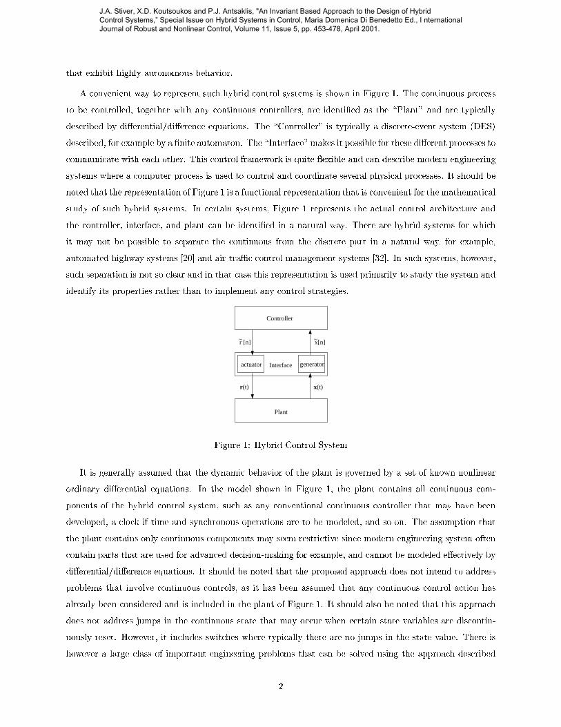
A convenient way to represent such hybrid control systems is shown in Figure 1. The continuous process

to be controlled, together with any continuous controllers, are identi�ed as the \Plant" and are typically

described by di�erential/di�erence equations. The \Controller" is typically a discrete-event system (DES)

described, for example by a �nite automaton. The \Interface" makes it possible for these di�erent processes to

communicate with each other. This control framework is quite exible and can describe modern engineering

systems where a computer process is used to control and coordinate several physical processes. It should be

noted that the representation of Figure 1 is a functional representation that is convenient for the mathematical

study of such hybrid systems. In certain systems, Figure 1 represents the actual control architecture and

the controller, interface, and plant can be identi�ed in a natural way. There are hybrid systems for which

it may not be possible to separate the continuous from the discrete part in a natural way, for example,

automated highway systems [20] and air-traÆc control management systems [32]. In such systems, however,

such separation is not so clear and in that case this representation is used primarily to study the system and

identify its properties rather than to implement any control strategies.

Controller

Interface

Plant

generatoractuator

r [n]~ x[n]~

r (t) x(t)

Figure 1: Hybrid Control System

It is generally assumed that the dynamic behavior of the plant is governed by a set of known nonlinear

ordinary di�erential equations. In the model shown in Figure 1, the plant contains all continuous com-

ponents of the hybrid control system, such as any conventional continuous controller that may have been

developed, a clock if time and synchronous operations are to be modeled, and so on. The assumption that

the plant contains only continuous components may seem restrictive since modern engineering system often

contain parts that are used for advanced decision-making for example, and cannot be modeled e�ectively by

di�erential/di�erence equations. It should be noted that the proposed approach does not intend to address

problems that involve continuous controls, as it has been assumed that any continuous control action has

already been considered and is included in the plant of Figure 1. It should also be noted that this approach

does not address jumps in the continuous state that may occur when certain state variables are discontin-

uously reset. However, it includes switches where typically there are no jumps in the state value. There is

however a large class of important engineering problems that can be solved using the approach described

2


in this paper. The primary emphasis is on understanding how the interface between the continuous and

the discrete part a�ects the properties of the hybrid system. This is one of the fundamental issues in the

theory of hybrid control systems. These concepts and methodologies may be used directly or indirectly in

the design of hybrid control systems, the latter in the case when the plant also contains discrete dynamics.

The interface plays a key role in determining the dynamic behavior of the hybrid control system. Here,

the interface has been chosen to be simply a partitioning of the state space (see Figure 2) and this is done

without loss of generality. If memory is necessary to derive an e�ective control law, it is included in the DES

controller and not in the interface. Also the piecewise continuous command signal issued by the interface

is simply a staircase signal as shown in Figure 3, not unlike the output of a zero-order hold in a digital

control system. Note that signals such as ramps, sinusoids, etc., can be generated if desired by including an

appropriate continuous system at (the input of) the plant. The simplicity of the interface with the resulting

bene�ts in identifying central issues and concepts in hybrid control systems is perhaps the main characteristic

of the approach.

X

h (x)1

h (x)2 h (x)3

h (x)4

Figure 2: Partition of the continuous state space

time

commandsignal

τ [1]cτ [2]c τ [3]c

Figure 3: Command signal issued by the interface

In this paper, we present a methodology to design the partition of the continuous state space based on

the natural invariants of the plant. Many times the partition of the state space is determined by physical

constraints and it is �xed and given. Here, we assume that we can select the partition and we focus on speci�c

problems for the interface design. Our approach leads to a systematic controller synthesis methodology that

is illustrated in the paper using several examples. More details of the invariant based approach can be found

in [25]. Earlier versions of this work have appeared in [28, 27, 29].

3


This paper contains a complete and self-contained description of the approach including a computational

procedure for implementation and illustrating examples. The contributions of the paper are the modeling

framework and the control design methodology based on the natural invariants for the continuous dynamics.

The methodology is justi�ed using theoretical results that explain precisely how the natural invariants are

used for controller design. Such invariant hypersurfaces can be obtained by solving analytically a partial

di�erential equation known as the characteristic equation of the system. The approach is illustrated with

two examples of a double and a triple integrator. Furthermore, a computational procedure for the numerical

implementation of the methodology which does not require the analytic solution of the characteristic equation

is presented. It should be noted that this computational procedure is based on quantization of the state

space which assumed to be bounded and therefore it does not address decidability and convergence issues.

The approach is illustrated with an example of an unmanned underwater vehicle.

The approach presented here not only represents a viable methodology to hybrid design, but also addresses

fundamental issues in hybrid system theory with respect to the partitioning of the continuous state space.

Similar issues arise in reachability analysis and veri�cation approaches that use continuous partitions based

on the concept of the ow, see for example [1, 23, 31]. The computational approach presented in this paper

is closely related to the computation of reachable sets for hybrid dynamical systems. that has received

extensive attention in recent years. A methodology for approximating reachable sets of piecewise-linear

system by polyhedra has been presented in [9]. Ellipsoidal techniques for reachability analysis of linear

time-varying systems have been proposed in [17]. It should be noted that our approach can be applied to

hybrid systems with nonlinear continuous dynamics an discrete control inputs. In the case when the invariant

hypersurfaces that partition the state space cannot be computed analytically, the propoped computational

procedure can be applied for approximation of the reachable sets.

In general the design of the interface depends not only on the plant to be controlled, but also on the

control policies available, as well as on the control goals to be attained. Certain control goals may require,

for example, detailed feedback information while for others coarser quantization levels of the signals may

be suÆcient. The former case corresponds to �ner partitioning of the feedback signal space, while the

latter corresponds to coarser partitioning. The fact that di�erent control goals may require di�erent types

of information about the plant is not surprising, as it is rather well known that to stabilize a system, for

example, requires less detailed information about the system's dynamic behavior than to do tracking. Note

that in general, the fewer the distinct regions in the partitioned signal space, the simpler (fewer states) the

resulting DES plant model will be, and this will result in a simpler DES controller design. Since the systems

to be controlled via hybrid controllers are typically complex, it is important to make every e�ort to use only

the necessary information to attain the control goals, as this leads to simpler interfaces that issue only the

necessary number of distinct symbols, and to simpler DES plant models and controllers. The question of

systematically determining the minimum amount of information needed from the plant in order to achieve

particular control goals using a �nite number of distinct control policies is an important and largely open

4


question; our work only partially resolves this question.

A great amount of research work has already been done in the hybrid systems area during the past

decade; see for example [4, 2, 5, 3, 8, 6]. A powerful approach that has been used extensively in the hybrid

system literature uses the continuous partition (partition of the continuous state space) to suppress the

continuous dynamics and to study the overall system in a discrete domain. A very important problem

that arises is whether there exist partitions of a continuous system that capture the behavior in such a

manner that preserve the important characteristics but result in simpli�ed system descriptions. The design

problem of continuous partitions is central in hybrid system and had been identi�ed as such as early as

1991 [26]. The problem of obtaining discrete abstractions of continuous systems is directly related to the

formal veri�cation techniques for analyzing hybrid systems. In the computer science community, hybrid

models are essentially extensions of �nite state machines that incorporate simple continuous dynamics [1].

Veri�cation algorithms are used to guarantee that the system model indeed satis�es the speci�cations. Since

hybrid systems have in�nite state spaces, the decidability of the veri�cation algorithms is studied using

discrete abstractions of hybrid systems. Veri�cation algorithms for hybrid systems investigate how the ow

of the continuous part interacts with certain regions in the state space. If it is assumed that the discrete

variables are �nite, then the decidability of the veri�cation algorithms depends on whether each individual

continuous component can be represented by a discrete abstraction preserving the behavior of interest.

Several computational approaches have been proposed to determine �nite bisimulations that are essentially

equivalence relations on the state space and de�ne continuous partitions [13, 18]. Methods for computing

continuous partitions based on approximations of the ow have also been considered [11]. Computational

algorithms for the use of the phase-space geometric description of dynamics have been developed in [33].

Related approaches using a feedback architecture of a continuous plant with a discrete-event controller have

appeared in [24, 30, 12, 19, 10, 16].

The paper is organized as follows. Section 2 presents the hybrid control system modeling. A methodology

to design the controller and the interface together based on the natural invariants of a plant is described

in Section 3. A methodology for optimizing the invariant based approach is discussed in Section 4. A

computational procedure for the implementation of the approach is presented in Section 5. Finally, some

concluding remarks are included in Section 6.

2 Hybrid Control System Modeling

2.1 Plant

The plant is in general a nonlinear, time-invariant system represented by a set of ordinary di�erential

equations.

_x(t) = f(x(t); r(t)) (1)

5


where x(t) 2 X and r(t) 2 R are the state and input vectors respectively, and X � <n;R � <m, with

t 2 (a; b) some time interval. It is assumed that for each �xed r(t) 2 R the function f(�; r(t)) : X ! X is

continuous and satis�es a Lipschitz condition on X. Then, for any x0 2 X the corresponding initial value

problem has a unique solution in the interval (a; b) (see for example [7]). Note that the plant input and state

are continuous-time vector valued signals.

The representation of the plant is quite general and can be used to describe a large class of systems that

includes time-invariant nonlinear systems and switching systems. For example, a linear switching system

consisting of m subsystems can be described by

_x(t) =mXi=1

ri(t)Aix(t)

where x 2 <n; ri : < ! f0; 1g;Pm

i=1 ri(t) = 1;8t 2 <; where ri(�1) = 1 implies that the system Ai is

actuated at time �1.

2.2 Controller

The controller is a discrete event system which is modeled as a deterministic automaton [14]. This automaton

is speci�ed by a quintuple, ( ~S; ~X; ~R; Æ; �), where ~S is the set of states, ~X is the set of plant symbols, ~R is

the set of controller symbols, Æ : ~S � ~X ! ~S is the state transition function, and � : ~S ! ~R is the output

function. The symbols in set ~R are called controller symbols because they are generated by the controller.

Likewise, the symbols in set ~X are called plant symbols and are generated based on events in the plant. The

action of the controller is described by the equations

~s[n] = Æ(~s[n� 1]; ~x[n]) (2)

~r[n] = �(~s[n]) (3)

where ~s[n] 2 ~S; ~x[n] 2 ~X, and ~r[n] 2 ~R. The index n speci�es the order of the symbols in the sequence. The

input and output signals associated with the controller are sequences of symbols. Tildes are used to indicate

a symbol valued set or sequence. For example, ~X is the set of plant symbols and ~x[n] is the nth symbol of

a sequence of plant symbols. Subscripts are also used, e.g. ~xi which denotes the ith member of the symbol

alphabet ~X.

2.3 Interface

The controller and plant cannot communicate directly in a hybrid control system because each utilizes a

di�erent type of signal. Thus an interface is required which can convert continuous-time signals to sequences

of symbols and vice versa. The way that this conversion is accomplished determines, to a great extent, the

nature of the overall hybrid control system. The interface consists of two simple subsystems, the generator

and actuator.

6


The generator issues symbols to the controller and plays the role of a quantizer of the signals analogous to

an A/D converter (sampler) in a digital control system. The actuator injects the appropriate control signal

into the plant and it is analogous to a D/A converter (which typically has zero-order hold) in a digital control

system. The generator and the actuator perform, however, more general functions than their counterparts

in a typical digital control system.

2.3.1 Plant Events and the Generator

The generator is the subsystem of the interface which converts the continuous-time output (state) of the

plant to an asynchronous, symbolic input for the controller. To perform this task, two processes must be

in place. First, a triggering mechanism is required which will determine when a plant symbol should be

generated. Second, a process to determine which particular plant symbol should be generated is required.

In the generator, the triggering mechanism is based on the idea of plant events. A plant event is simply

an occurrence in the plant, an idea borrowed from the �eld of discrete event systems. In the case of

hybrid control, a plant event is de�ned by specifying a hypersurface which separates the plant's state space.

The plant event occurs whenever the plant state trajectory crosses this hypersurface. The basis for this

de�nition of a plant event is that an event is considered to be the realization of a speci�ed condition. This

condition can be given as an open region of the state space, separated from the remainder of the state

space by a hypersurface. If the state crosses the hypersurface into the given open region, the event has

occurred. Mathematically, the set of plant events recognized by the generator is determined by a set of

smooth functionals, fhi : <n ! <; i 2 Ig, de�ned on the state space of the plant. Each functional must

satisfy the condition,

rxhi(�) 6= 0;8� 2 N (hi) (4)

which ensures that the null space of the functional, N (hi) = f� 2 <n : hi(�) = 0g, forms an n�1 dimensional

smooth hypersurface separating the state space.

Let the sequence of plant events be denoted by e, where e[n] = i means that the nth plant event was

triggered by crossing the hypersurface de�ned by hi. Let the sequence of plant event instants be given by

�e, where �e[n] is the time of the nth plant event and �e[0] = 0. By de�nition, these sequences satisfy the

following conditions.

e[n] = i)

8>>><>>>:

hi(x(�e[n])) = 0

9 Æ1 > 0 s.t. 8�; 0 < � < Æ1;�hi(x(�e[n] + �)) < 0

9 Æ2 > 0 s.t. 8�; 0 < � < Æ2;�hi(x(�e[n]� Æ2)) > 0;�hi(x(�e[n]� �)) � 0

(5)

and

8n; �e[n] < �e[n+ 1] _ (�e[n] = �e[n+ 1] ^ e[n] < e[n+ 1]) (6)

The �rst group, equation (5), contains three conditions: (i) at the time of the plant event the plant state lies

on the triggering hypersurface, (ii) immediately after the event the plant state lies on the negative (positive)

7


side of the triggering hypersurface, and (iii) prior to reaching the triggering hypersurface the plant state lied

on the positive (negative) side. The fourth condition, equation (6) concerns the ordering of the sequences.

It requires that plant events be ordered chronologically and simultaneous plant events be ordered according

to their number, that is the value of i.

An alternative, and perhaps simpler, way of expressing the conditions of (5) is by the condition, hi(x(t)) =

0; ddthi(x(t)) 6= 0; where t = �e(n)8n. In this case the assumption is made that the derivative is nonzero, that

is ddthi(x(t)) 6= 0 at the crossing. Note however that these conditions do not take into account the case where

the crossing occurs exactly at an in ection point. When ddthi(x(t)) = 0, one must use (5). Alternatively, the

conditions described by equation (5) can be expressed by

9n > 0; hi(x(t)) =d

dthi(x(t)) = : : : =

dn�1

dtn�1hi(x(t)) = 0;

dn

dtnhi(x(t)) 6= 0:

A plant event will only cause a plant symbol to be generated if the hypersurface is crossed in the negative

direction. The reason for this is that in many applications sensors only detect when a threshold is crossed

in one direction, e.g. a thermostat. When the hypersurface is crossed in the opposite direction the event is

silent, and for convenience, assume that a null symbol, �, is generated. At each time in the sequence �e[n],

a plant symbol is generated according to the function �i : N (hi) ! ~X . The sequence of plant symbols can

now be de�ned as

~x[n] =

8<:

�i(x(�e[n])) nonsilent event

� silent event(7)

where i identi�es the hypersurface which was crossed. Alternatively one could select the interface to gen-

erate information bearing symbols when crossed in either direction. Note that the symbol represents the

hypersurface that which was crossed by the state x(t) and does not depend on the point of the crossing.

2.3.2 The Actuator

The actuator converts the sequence of controller symbols to a plant input signal, using the function : ~R!<m, as follows.

r(t) =

1Xn=0

(~r[n])I(t; �c[n]; �c[n+ 1]) (8)

where I(t; �1; �2) is a characteristic function taking on the value of unity over the time interval [�1; �2) and

zero elsewhere. �c[n] is the time of the nth control symbol which is based on the sequence of plant symbol

instants, de�ned in equation (5), according to

�c[n] = �e[n] + �d (9)

where �d is the total delay associated with the interface and controller. Following the occurrence of a plant

event, it takes a time of �d for a new control policy to be used by the plant. It will be assumed that

�e[n] < �c[n] < �e[n+ 1].

8


The plant input, r(t), can only take on certain constant values, where each value is associated with a

particular controller symbol. Thus the plant input is a piecewise constant signal which may change only

when a controller symbol occurs.

Remark In the interface a delay, �d, was introduced. The presence of the delay is necessary for two

reasons. First, from a practical point of view, the generator will not be able to detect an event until after

the state has actually crossed the hypersurface. Second, if a nonzero delay is not used, it is possible the

di�erential equation (1) will exhibit solutions that switch between di�erent control policies in�nitely many

times in a �nite time interval. Such behavior does not occur in physical systems. Systems capable of

exhibiting such behavior are referred to as Zeno systems. In supervisory hybrid control systems, we want

the systems to be non-Zeno. It is of course possible for two plant events to occur within the period of a

single delay. In such a case each event will be acted upon, in turn, �d units of time after it occurs. In

this way the delay can pose a problem for the controller, but it is unavoidable as real systems cannot react

instantaneously.

3 Invariant Based Approach

Here a methodology is presented to design the controller and the interface together based on the natural

invariants of a plant described in Equation (1). In particular, this section discusses the design of the generator,

which is part of the interface, and the design of the controller. We assume that the plant is given, the set

of available control policies is given, and the control goals are speci�ed as follows. Each control goal for the

system is given as a starting set and a target set, each of which is an open subset of the plant state space.

To realize the goal, the controller must be able to drive the plant state from anywhere in the starting set

to somewhere in the target set using the available control policies. Generally, a system will have multiple

control goals. To successfully control the plant, the controller must know which control policy to apply

and when to apply it. The controller receives all its information about the plant from the generator, and

therefore the generator must be designed to provide that information which the controller requires.

We propose the following solution to this design problem. For a given target region, identify the states

which can be driven to that region by the application of a single control policy. If the starting region is

contained within this set of states, the control goal is achievable via a single control policy. If not, then this

new set of states can be used as a target region and the process can be repeated. This will result in a set

of states which can be driven to the original target region with no more than two control policies applied in

sequence. This process can be repeated until the set of states, for which a sequence of control policies exists

to drive them to the target region, includes the entire starting region (provided the set of control policies

is adequate as mentioned below). When the regions have been identi�ed, the generator is designed to tell

the controller, via plant symbols, which region the plant state is currently in. The controller will then call

9


for the control policy which drives the states in that region to the target region. Note that similar methods

based on backward analysis of the dynamics have been discussed in [23, 31].

3.1 Generator Design

To describe the regions mentioned above, we use the concept of the ow [22]. Let the ow for the plant (1)

be given by Fk : X�< ! X, where

x(t) = Fk(x(0); t): (10)

The ow represents the state of the plant after an elapsed time of t, with an initial state of x(0), and with

a constant input of (~rk). Since the plant is time invariant, there is no loss of generality when the initial

state is de�ned at t = 0. The ow is de�ned over both positive and negative values of time. The ow can

be extended over time using the forward ow function, F+k : X ! P(Xn) where P(Xn) denotes the power

set of Xn, and the backward ow function, F�k : X! P(Xn), which are de�ned as follows.

F+k (�) =

[t�0

fFk(�; t)g (11)

F�k (�) =[t�0

fFk(�; t)g (12)

The backward and forward ow functions can be de�ned on an arbitrary set of states in the following natural

way.

F+k (A) =

[

�2A

fF+k (�)g (13)

F�k (A) =[

�2A

fF�k (�)g (14)

where A � X. For a target region, T , F�k (T ) is the set of initial states from which the plant can be driven

to T with the input (~rk). In addition, F+k (T ) is the set of states which can be reached with input (~rk) and

an initial state in T . Note that the backward and forward ow functions applied on set of states correspond

to the precondition and postcondition operators used in veri�cation algorithms of hybrid systems [1].

Now a generator design procedure can be described using the backward ow function. This is a prelimi-

nary procedure, upon which the �nal design method, developed subsequently, is based. For a given starting

region, S � X, and target region, T � X, use the following algorithm.

1. If S � T , stop.

2. Identify the regions, F�k (T );8~rk 2 ~R.

3. Let T =[

~rk2 ~R

F�k (T )

4. Go to 1.

10


There are two problems associated with this algorithm as stated. First, it will not stop if there is no sequence

of available control policies which will achieve the control goal, and second, actually identifying the regions

given by the ow functions is quite involved. The �rst issue is related to the adequacy of the available control

policies and will not be dealt with here. The second problem will be addressed. The diÆculty in identifying

a region given by a ow function is integrating over all the points in the target region. In the generator

design procedure developed here, we will concentrate on �nding a subset of the region F�k (T ), rather than

the region itself. By de�nition, all the trajectories passing through F�k (T ) lead to the target region, T , and

therefore all the trajectories found in a subset of F�k (T ) will also lead to the target. Here, we will focus on

identifying subsets of F�k (T ) which we call common ow regions (CFR). Common ow regions are bounded

by invariant manifolds and an exit boundary. The invariant manifolds are used because the state trajectory

can neither enter nor leave the common ow region through an invariant manifold. The exit boundary is

chosen as the only boundary through which state trajectories leave the common ow region.

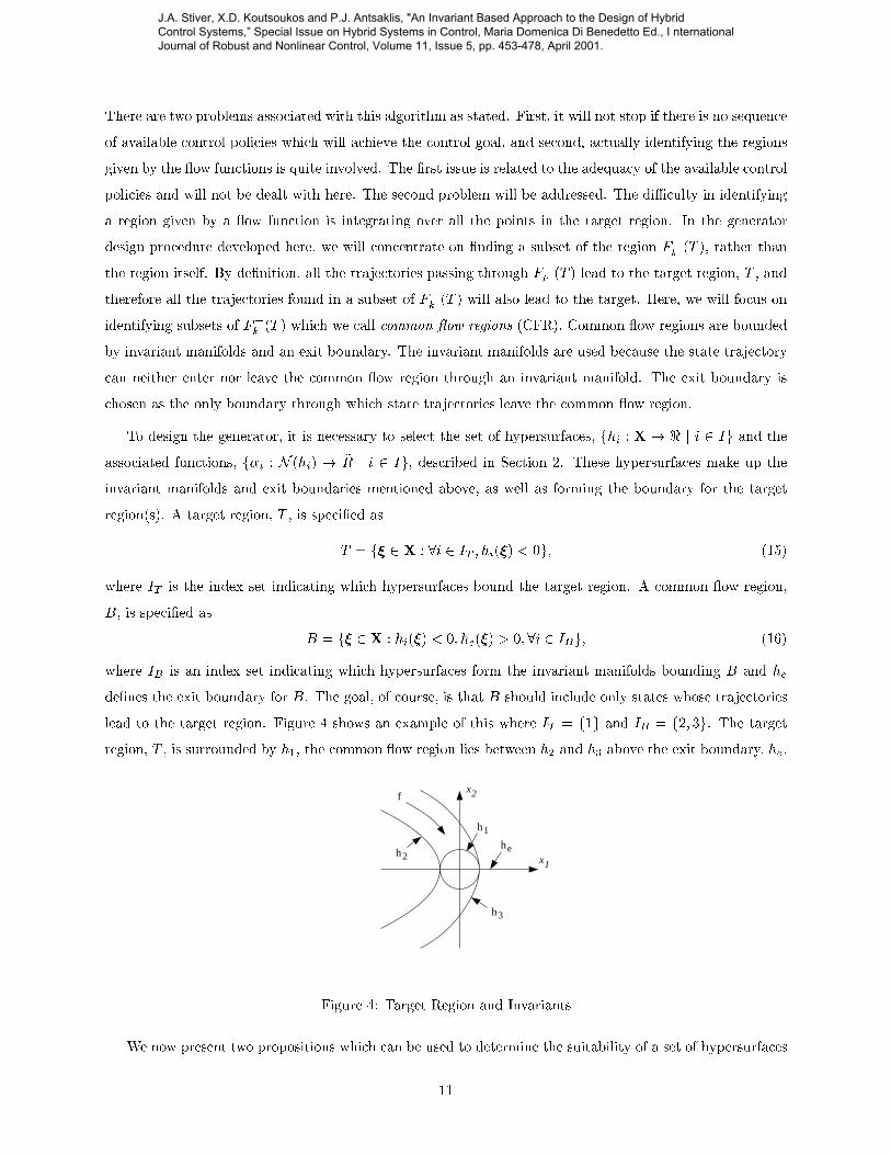
To design the generator, it is necessary to select the set of hypersurfaces, fhi : X ! < j i 2 Ig and the

associated functions, f�i : N (hi) ! ~R j i 2 Ig, described in Section 2. These hypersurfaces make up the

invariant manifolds and exit boundaries mentioned above, as well as forming the boundary for the target

region(s). A target region, T , is speci�ed as

T = f� 2 X : 8i 2 IT ; hi(�) < 0g; (15)

where IT is the index set indicating which hypersurfaces bound the target region. A common ow region,

B, is speci�ed as

B = f� 2 X : hi(�) < 0; he(�) > 0;8i 2 IBg; (16)

where IB is an index set indicating which hypersurfaces form the invariant manifolds bounding B and he

de�nes the exit boundary for B. The goal, of course, is that B should include only states whose trajectories

lead to the target region. Figure 4 shows an example of this where IT = f1g and IB = f2; 3g. The targetregion, T , is surrounded by h1, the common ow region lies between h2 and h3 above the exit boundary, he.

x

x1

2

h1

h2

h3

f

he

Figure 4: Target Region and Invariants

We now present two propositions which can be used to determine the suitability of a set of hypersurfaces

11


to achieve our goal of identifying a common ow region. In di�erent situations, one of the propositions may

be easier to apply than the other. The following propositions give suÆcient conditions for the hypersurfaces

bounding B and T to ensure that all state trajectories in B will reach the target region.

Proposition 1 Given the following:

1. A ow generated by a smooth vector �eld, fk

2. A target region, T � X

3. A set of smooth hypersurfaces, hi; i 2 IB � 2I

4. A smooth hypersurface (exit boundary), he

such that B = f� 2 X : hi(�) < 0; he(�) > 0;8i 2 IBg 6= ;. For all � 2 B there is a �nite time, t, such that

for the ow generated by fk we have Fk(�; t) 2 T , if the following conditions are satis�ed:

1. r�hi(�) � f(�) = 0;8i 2 IB

2. 9� > 0;r�he(�) � f(�) < ��;8� 2 B

3. B \ N (he) � T

Proof: The proof of this proposition is straightforward. The �rst condition of the proposition, which can

be rewritten asdhi(x(t))

dt= 0; (17)

precludes the state trajectory crossing any hypersurface indexed by the set IB , thus ensuring no trajectory

in B will leave B except through the remaining boundary. The second condition, which can be rewritten as

dhe(x(t))

dt< ��; (18)

ensures that within a �nite time,

t <he(�)

�; (19)

the trajectory at � 2 B will cross the exit boundary. The �nal condition guarantees that any trajectory

leaving B through the exit boundary will be in the target region when it does so. Together these conditions

are suÆcient to guarantee that any state in B will enter the target region in �nite time. 2

The second proposition uses a slightly di�erent way of specifying a common ow region. In addition to

the invariant manifolds and the exit boundary, there is also a cap boundary. The cap boundary is used to

obtain a common ow region which is bounded. So for this case

B = f� 2 X : hi(�) < 0; he(�) > 0; hc(�) < 0;8i 2 IBg: (20)

12


Proposition 2 Given the following:

1. A ow generated by a smooth vector �eld, fk

2. A target region, T � X

3. A set of smooth hypersurfaces, hi; i 2 IB � 2I

4. A smooth hypersurface (exit boundary), he

5. A smooth hypersurface (cap boundary), hc

such that B = f� 2 X : hi(�) < 0; he(�) > 0; hc(�) < 0;8i 2 IBg 6= ; and B (closure of B) is compact. For

all � 2 B there is a �nite time, t, such that Fk(�; t) 2 T , if the following conditions are satis�ed:

1. r�hi(�) � f(�) = 0;8i 2 IB

2. r�hc(�) � f(�) < 0;8� 2 B \ N (hc)

3. B \ N (he) � T

4. There are no limit sets in B

Proof: As in Proposition 1, the �rst condition precludes the state trajectory crossing any hypersurface

indexed by the set IB , thus ensuring no trajectory in B will leave B except through one of the remaining

boundaries. The second condition, which can be rewritten as

dhc(x(t))

dt< 0; (21)

ensures that no trajectory can leave B through the cap boundary. Thus, the exit boundary provides the

only available egress from B. The third condition guarantees that any trajectory leaving B through the

exit boundary will be in the target region when it does so. The �nal condition permits the application of a

previously known result [21], stating that any state within a compact set without limit sets will leave that

compact set in �nite time. 2

Consider the hypersurfaces de�ned by fhi : i 2 IBg. These hypersurfaces must �rst be invariant underthe vector �eld of the given control policy, f . This can be achieved by choosing them to be integral manifolds

of an n� 1 dimensional distribution which is invariant under f . An n� 1 dimensional distribution, �(x), is

invariant under f if it satis�es

[f(x);�(x)] � �(x); (22)

where the [f(x);�(x)] indicates the Lie bracket. Of the invariant distributions, those that have integral

manifolds as we require, are exactly those which are involutive (according to Frobenius). This means

Æ1(x); Æ2(x) 2 �(x)) [Æ1(x); Æ2(x)] 2 �(x): (23)

13


Therefore by identifying the involutive distributions which are invariant under the vector �eld, f , we have

identi�ed a set of candidate hypersurfaces. For details of these relationships between vector �elds and

invariant distributions, see [15]. Since an n � 1 dimensional involutive distribution can be de�ned as the

span of n� 1 vector �elds, over each of which it will then be invariant, and the control policy only gives one

vector �eld, f , there will be more than one family of hypersurfaces which are all invariant under f . The set

of all invariant hypersurfaces can be found in terms of n� 1 functionally independent mappings which form

the basis for the desired set of functionals, fhi : i 2 IBg. This basis is obtained by solving the characteristic

equationdx1f1(x)

=dx2f2(x)

= � � � = dxnfn(x)

(24)

where fi(x) is the ith element of f(x). The invariant hypersurfaces that will be are used to partition the

state space are determined by selecting appropriately the parameters of the basis based on the target region.

The approach is illustrated with two examples of a double and triple integrator in the next section.

3.2 Controller Design

In previous work using this framework for hybrid control systems, the interface was assumed to be given

and the controller was designed using the given plant and interface; see [30]. In those cases, the plant and

interface were modeled as a discrete event system, called the DES plant model, and existing DES controller

design techniques were adapted and used to obtain a controller. The drawback was that there was no

guarantee that the desired behavior could be achieved with the given plant and interface. Now, with the

generator design technique described in Section 3.1, the controller design is anticipated by the design of

the interface. This represents an improvement over the previous situation because now there is no question

that the control goal can be achieved once the interface has been successfully designed, and furthermore the

actual controller design has been largely determined by the interface design.

Once the interface has been designed as described in Section 3.1, the design of the controller involves

two steps. Here, it is assumed that adequate control policies are available. The �rst step is to construct one

subautomaton for each control goal. This is the step which is already determined by the interface design.

The second step is the connection of these subautomata to create a single DES controller. This step will

depend upon the order in which the simpler control goals are to be achieved. For example, if a chemical

process is to produce a sequence of di�erent products, then each subautomaton in the controller would be

designed to produce one of the products, and these subautomata would be connected to produce the products

in the desired sequence. The hypersurfaces in the generator divide the state space of the plant into a number

of cells. Two states are in the same cell exactly when they are both on the same side (positive or negative)

with respect to each hypersurface. States which lie on a hypersurface are not in any cell.

The �rst step in creating the controller is the construction of the subautomata, one for each individual

control goal. Each subautomaton is constructed in the following way.

14


i. Create a controller state to represent each cell.

ii. Place transitions between states which represent adjacent cells.

iii. Label each transition with the plant symbol which is generated by the hypersurface separating the

associated cells.

We now have a subautomaton which can follow the progress of the plant state as it moves from cell to

cell. Next the controller output function must be designed for each subautomaton. The controller symbol

output by a given controller state depends on which common ow region contains the associated cell. Each

common ow region was constructed using a speci�c control policy, and the control symbol which initiates

that control policy should be output by controller states representing cells contained in that common ow

region. However, in general, common ow regions will overlap, meaning a given cell can lie in more than

one common ow region. In such cases treat the cell as lying within the common ow region which is closest

to the target region. Distance, in this case, is the number additional control policies which must be used

to reach the target region. If common ow regions are both the same distance, then the choice is arbitrary,

though the common ow region which is favored in one case must then be favored in all such cases. States

which represent cells not contained in any common ow region or target region will never be visited and can

thus be deleted.

Once the individual subautomata have been constructed they must be connected to form a single con-

troller. This can be accomplished by following these steps for each subautomaton.

i. Remove the state(s) which represent cells in the target region as well all transitions emanating from

such states.

ii. Connect the dangling transitions to states in the subautomaton which achieves the next desired control

goal. The connections will be to the states which represent the same cells as the states which were

removed.

In this way, as soon as one control goal is achieved, the system will begin working on the next one. The

actual order in which each control goals are pursued is up to the designer.

3.2.1 Example - Double Integrator

Consider the double integrator example. Suppose we are given the plant,

_x(t) =

24 0 1

0 0

35x(t) +

24 0

1

35 r(t); (25)

three available control policies,

r(t) 2 f�1; 0; 1g; (26)

15


and the following control goal: drive the plant state to the interior of the unit circle from any initial point.

So the starting set consists of the entire state space, and the target set is

T = f� 2 X : �21 + �22 < 1g: (27)

The target set is bounded by the hypersurface given by

hT (�) = �21 + �22 � 1 (28)

The �rst step is to calculate the invariants which can be used to obtain hypersurfaces. There are three

families of invariants, one for each of the three control policies.

�(�1 + 1

2�22 + c1) (29)

�(�1 � 1

2�22 + c2) (30)

�(�2 + c3) (31)

The �rst hypersurface, h1, is used to identify the target region.

h1(�) = hT (�) = �21 + �22 � 1 (32)

A common ow region entering T under the �rst control policy, r(t) = �1, is bounded by

h2(�) = ��1 � 1

2�22 � :9 (33)

h3(�) = �1 +1

2�22 � :9 (34)

and

he(�) = h4(�) = �2 + :1 (35)

These hypersurfaces satisfy Proposition 1. Identify this common ow region as B1.

B1 = f� : hi(�) < 0; h4(�) > 0; i 2 f2; 3gg (36)

Likewise, a common ow region entering T under the third control policy is bounded by

h5(�) = ��1 + 1

2�22 � :9 (37)

h6(�) = �1 � 1

2�22 � :9 (38)

and

he(�) = h7(�) = ��2 + :1 (39)

Identify this common ow region as B2.

B2 = f� : hi(�) < 0; h7(�) > 0; i 2 f5; 6gg (40)

16


Figure 5 (i) illustrates what we have so far. Now the target can be extended to include B1 or B2 and more

common ow regions can be obtained. Let the new target be given by T 0 = T [B1. A common ow region

entering T 0 under the second control policy is bounded by choosing

IB3= f7g (41)

and e = 2. A common ow region entering T 00 = T 0 [ B3 under the third control policy is bounded by

choosing

IB5= f6g (42)

and e = 7. Figure 5 (ii) gives a �nal picture of the hypersurfaces and regions involved in this example.

ξ

ξ1

2

h1h2

h3

h6

h5

B1

B2

ξ

ξ1

2

B1

B2

B3

B4B5

B6

T

x 1

~

x 1

~

x2

~

x 7

~

s 3

s T

s 4

s 1

s 2

x 6

~

s 5

x 4

~

s 6

(i) (ii) (iii)

Figure 5: (i) Target Region and Invariants, (ii) Final Regions for Double Integrator, (iii) Controller

There is only one control goal for this example and therefore the entire controller will consist of a single

subautomaton. Start by creating a controller state ~sT which is associated with the target region. Two

common ow regions, labeled B1 and B2, were identi�ed which lead to the target region. So create two more

controller states, ~s1 and ~s2. B1 consists of the trajectories which reach the target region under control policy

~r1 and therefore �(~s1) = ~r1, likewise �(~s2) = ~r3. Connect ~s1 to ~sT with a transition labeled ~x1 which is

generated when the plant state crosses h1 to enter the target region. Do the same for ~s2. Next, create ~s3 to

go with B3, and add a transition to ~s1 labeled ~x2. When all the common ow regions have their associated

states and transitions the controller shown in Figure 5 (iii).

3.2.2 Example - Triple Integrator

With the double integrator example, it is easy to see how the invariant surfaces are used. The technique can

also be used in more complicated cases where it is not so intuitively obvious. Consider the triple integrator,

_x(t) =

26664

0 1 0

0 0 1

0 0 0

37775x(t) +

26664

0

0

1

37775 r(t); (43)

17


with the same three available control policies,

r(t) 2 f�1; 0; 1g: (44)

This time the control goal is to drive the state to the unit sphere from any initial state. First �nd a basis

for the invariants by solving the characteristic equation

dx1x2

=dx2x3

=dx3r

(45)

Two functions are obtained,

ha(�) = r�2 � 1

2�23 + c1 (46)

hb(�) = r2�1 +1

3�33 � r�2�3 � rc2; (47)

where r is the input (control policy) and c1 and c2 are arbitrary constants. Example hypersurfaces for r = 1

and c1 = c2 = 0 are shown in Figure 6 (i) and 6 (ii).

-10-5

05

10

0

10

20

30

40

50-10

-5

0

5

10

x1x2

x3

-10-5

05

10

-10

-5

0

5

10

-600

-400

-200

0

200

400

x3x2

x1

(i) (ii)

Figure 6: (i) Invariant for ha, (ii) Invariant for hb

The target region is bounded by the hypersurface, h1, i.e. IT = f1g.

h1(�) = �21 + �22 + �23 � 1 (48)

Now identify a common ow region which enters the target region under the input r(t) = 1. The following

hypersurfaces are used.

h2(�) = ��2 + 1

2�23 �

p2 (49)

h3(�) = �2 � 1

2�23 �

p2 (50)

h4(�) = �1 +1

3�33 � �2�3 �

p2 (51)

h5(�) = ��1 � 1

3�33 + �2�3 �

p2 (52)

The common ow region runs through the origin, where the target is centered, and the constant values,

�p2, where chosen so that the common ow region passes through the target.

18


4 Optimizing the Invariant Based Approach

The invariant based approach to interface design produces a set of hypersurfaces in the state space of the

plant. These hypersufaces form the boundaries of common ow regions (CFRs), which are regions of the

state space where all the trajectories ow to the same subsequent CFR under a particular control policy.

By driving the state through a sequence of CFRs the controller can eventually drive it to the target region.

Since each CFR is associated with a unique control policy, the controller has only determine the CFR in

which the current state resides and apply the associated policy.

In general, however, the CFRs will intersect each other, and therefore the plant state may well lie in

multiple CFRs simultaneously. In such cases the controller must choose one of the CFRs in order to decide

which control policy to apply. The controller design procedure described here bases this choice on the

optimization of some measure of performance. The particulars of the measure used are not important to

the design procedure provided they can be expressed as a cost associated with each CFR. The controller

will choose to drive the plant through the sequence of CFRs which reaches the target region with the lowest

total cost.

4.1 Problem Formulation

Assume the invariant based design scheme has been completed. The result is a set of hypersurfaces which

identify a set of CFRs. The set of CFRs is denoted by T where T � P(X). For each CFR, Ti 2 T , threefunctions are de�ned.

depth(Ti) 2 f0::Dg depth of CFR Ti

cost(Ti) 2 < cost of traversing Ti

CP(Ti) 2 f0::Kg control policy for Ti

next(Ti) 2 T CFR reached via CFR Ti

These functions are determined by the interface design algorithm. The depth of a CFR refers to the

number of CFRs traversed before reaching the target. The target has a depth of 0. The cost of traversing a

CFR will depend on the particular control problem, it can re ect the control e�ort required, the performance

of the plant when its state lies in the CFR, etc. The function, next, indicates which CFR is reached from

the present CFR. This function can be extended to in the following way.

next0(Ti) = Ti

next1(Ti) = next(Ti)

next2(Ti) = next(next(Ti))...

19


The set of hypersurfaces which form the boundaries for the various CFRs will form a set of open regions,

S � P(X), in the plant state space. Each of these open regions may belong to a number of CFRs. Through

observation of the sequence of plant events the controller knows which of these open regions contains the

plant state an must decide which control policy to apply. The following function identi�es the CFRs which

contain a given open region, S.

CFR(S) � T CFRs containing region S

The relation Ti 2 CFR(S) is equivalent to S � T .

4.2 Optimization

When the plant state is in the open region, S, the controller will select from among the CFRs in the set

CFR(S), the CFR which provides the lowest total cost to reach the target. The total cost to reach the target

from CFR Ti is given by the following summation.

depth(Ti)Xj=0

cost(nextj(Ti)) (53)

Therefore when the plant state is in the open region S, the controller will apply the control policy

CP (Ti)

where Ti is determined by the following optimization,

minTi2CFR(S)

depth(Ti)Xj=0

cost(nextj(Ti)): (54)

4.3 Designing the Optimal Controller

The most straightforward way to implement the controller is to create an automaton with one state for each

of the open regions in the set, S. Then as the plant evolves and produces plant symbols, the controller

can track the plant state and provide the optimal control policy as de�ned by (54). Therefore the output

function for the controller is given by

�(S) = CP (Ti)

where Ti is given by (54).

5 A Computational Procedure for the Invariant Based Approach

The design procedure presented in this paper is straightforward, but not computationally easy. For these rea-

sons it is desirable to automate the procedure on a computer. Here a simple automation scheme is presented

20


along with results for an example of an unmanned underwater vehicle (UUV). The UUV demonstrates that

the algorithm also works for more complex systems where implementation via human calculation is allmost

impossible. The procedure was developed in [25] and is similar to the backward analysis approach in formal

veri�cation [1].

5.1 The Algorithm

The computerized procedure does not �nd the hypersurfaces which bound the common ow regions, but

rather seeks to identify the regions directly. This is achieved by simply back-calculating the state trajectories

from the target region and recording the states which are encountered. It requires quantizing and bounding

the state space so that the computer will have a �nite number of state values to deal with.

To use the program the designer must choose the quantization levels for each state, �xi, and the range

of each state, xi;min and xi;max. These choices lead to a quantization of the plant state space into a number

of n-dimensional cells. The number of cells is given by

Yi

xi;max � xi;min

�xi(55)

As can be seen, the order of the computational complexity is qn, where q is the number of quantization

levels and n is the number of states. This limits the size of systems which can be handled in a reasonable

amount of time. The limit depends on the computational power available and on the designer's idea of what

is \reasonable". For example, for the UUV system we have qn � 105.

After the designer has quantized and bounded the state space, the procedure requires two additional

pieces of information from the designer. The set of available plant inputs (control policies) must be provided

and the target region must be speci�ed in terms of the cells. That is, the cells which lie in the target region

must be identi�ed as such by the designer. Once the procedure has the requisite information, it proceeds

according to the algorithm outlined by the owchart shown in Figure 7. The algorithm shown in the chart

will locate all cells from which it is possible to reach the target region via the application of any one control

policy. The procedure resets the target region to include all these cells and then repeats the algorithm. In this

way, all cells from which it is possible to reach the original target via the application of two control policies

in sequence are identi�ed. The algorithm will be repeated as many times as the designer has speci�ed. When

it terminates, each cell is marked with the control policy which should be used to reach the target, either

directly or as the �rst in a sequence of control policies.

There is generally more than one trajectory which can be followed from an initial point to a target region.

A question therefore arises regarding which of the possible trajectories should be followed. A trajectory that

satis�es a desirable cost criterion can be obtained using the optimization procedure presented in Section 4.

An optimization procedure can be formulated by de�ning a cost function to associate costs with trajectories.

Then, when the algorithm calculates a trajectory it will also calculate the associated cost and compare it to

21


BEGIN

Get first cellin target region

Calculate trajectoryleading to current cell

with current policy

Morecells?

Get next cell

Morepolicies?

Mark all unmarkedcells on trajectorywith current policy

Get nextcontrol policy

END

Yes

Yes

No

No

Get firstcontrol policy

Figure 7: Algorithm

any trajectories which have been found previously. The trajectory with the lowest cost would be retained.

In the UUV example, the chosen trajectory was simply the �rst one which was found by the algorithm.

The procedure has a requirement that the search area of the state space be bounded, and this requirement

can be used to an advantage by the designer. First, the speed of the procedure is increased by shrinking

the size of the state space which is searched. In addition, by carefully choosing the shape of the search

area, the designer can coerce the procedure into �nding control laws which satisfy a desired property. For

example, in a forbidden region problem, the undesirable region is placed outside the bounds of the search

area and therefore no trajectories in this region will be considered. This idea can be extended to force the

procedure to �nd a solution which follows a rough path from the starting set to the target set. The designer

can accomplish this by de�ning a \tube" through the state space from the starting set to the target set, and

using the boundary of the tube as the boundary of the search area in the state space. Of course, reducing

the search area reduces the number of possible solutions and it is possible that no solutions lie in a particular

region of the state space.

5.2 Example - Unmanned Underwater Vehicle

Unmanned underwater vehicles (UUV) have a wide variety of practical usages in missions where it is dan-

gerous or impossible to send a manned underwater vehicle. Exploration, search and rescue, salvage, mine

22


disposal, and demolition are some examples of the uses of UUV's. The UUV shows that the program

described above can also solve a reasonably complex, nonlinear system.

This example used a simpli�ed model of a six-degree-of-freedom UUV depicted in Figure 8. The three

types of linear displacement are surge, sway, and heave, which represent translation in the x, y, and z,

directions respectively. The three types of angular displacement are roll, pitch, and yaw. The model employed

here has six states which are the time derivatives of the three linear displacements and the magnitudes of the

three angular displacements. By expanding to a nine state model, the magnitudes of the linear displacements,

could also be included. They are omitted here to simplify the control problem and because they do not a�ect

the dynamics of the UUV.

zx

y

θx

θy

θzrudder

sternplanescrew

Figure 8: Unmanned Underwater Vehicle

The UUV model has three inputs which control the rudder, stern plane, and screw. The following table

summarizes the variables of the model.

x surge rate (forward speed)

y sway rate (lateral speed)

z heave rate (vertical speed)

�x roll angle in radians

�y pitch angle in radians

�z yaw angle in radians

ux screw

uy stern plane angle

uz rudder angle

The simpli�ed model is as follows.

_x = �x+ ux

_y = �y + 0:01xuy

_z = �z + 0:01xuz (56)

_�y = 0:15xuy

_�z = 0:15xuz

23


Notice that the roll angle is not included in the model. It is assumed that the center of mass of the UUV is

suÆciently far beneath the center of buoyancy so that the roll angle is always zero.

To control the UUV, the actuator can implement ten di�erent control policies. The policies allow various

combinations of two screw speeds (on and o�), three stern plane positions (up, level, down), and three rudder

positions (left, right, straight).

r(t) =

26664

ux

uy

uz

37775 (57)

The controller has ten control policies to choose from. These policies are obtained by combining two

propeller speeds ux 2 f0; 1g, three stern plane angles uy 2 f�10; 0; 10g, and three rudder angles uz 2f�10; 0; 10g. Of the control policies with r1 = 0, only the one with r2 = r3 = 0 is kept, reducing the total

number of control policies from eighteen to ten.

The unmanned underwater vehicle example is suÆciently complex, with �ve states, three inputs, and

non-linear dynamics, that the design methodology of this paper cannot be carried out without some form of

systematic, automated procedure.

The procedure is used to design a controller for the UUV and then the design is evaluated through

simulation. The state space of the UUV plant is quantized and bounded as follows.

x1;min = 0 x1;max = 1 �x1 = 0:1

x2;min = �0:5 x2;max = 0:5 �x2 = 0:2

x3;min = �0:5 x3;max = 0:5 �x3 = 0:2

x4;min = ��=2 x4;max = �=2 �x4 = �=20

x5;min = ��=2 x5;max = �=2 �x5 = �=20

The target region consists of the following interval.26666666664

0:1

�0:1�0:1��=40��=40

37777777775

< x <

26666666664

0:2

0:1

0:1

�=40

�=40

37777777775

(58)

The results of two simulations are presented here. The two trials have the following initial conditions.

x =

26666666664

surge

sway

heave

pitch

yaw

37777777775

;x1 =

26666666664

0:8

0

0

�1:171:00

37777777775

;x2 =

26666666664

0:2

0:4

0

0:67

�1:50

37777777775

(59)

24


Results of two trials are shown in Figure 9 (i) and 10. Each �gure consists of four graphs. The graph in the

upper left shows the surge, sway, and heave over time. The graph in the upper right shows the pitch and

yaw over time. The trajectories on these two graphs can be distinguished by noting the initial conditions.

The two lower graphs show the control signal. On the lower left is the propeller speed which is either 0 or

1. The segments which appear to overlap reveal the presence of chattering (due to quantization). The �nal

graph shows the stern plane angle and the rudder angle. In Figure 9, the stern plane switches between 0 and

10 and the rudder angle switches between �10 and 0. In Figure 10 these are reversed. As can be seen, the

basic control strategy which developed is simply to accelerate and turn until the pitch and yaw are within

the bounds of the target region, and then coast until the forward speed is also in the target.

0 100 200 300−0.5

0

0.5

1

1.5x, y, and z

0 100 200 300−1.5

−1

−0.5

0

0.5

1

pitch and yaw

0 100 200 300−0.5

0

0.5

1

1.5u_x

0 100 200 300−15

−10

−5

0

5

10

u_y and u_z

Figure 9: UUV Simulation #1

0 100 200 300−0.5

0

0.5

1

1.5x, y, and z

0 100 200 300−1.5

−1

−0.5

0

0.5

1

pitch and yaw

0 100 200 300−0.5

0

0.5

1

1.5u_x

0 100 200 300−15

−10

−5

0

5

10

u_y and u_z

Figure 10: UUV Simulation #2

25


6 Conclusions

An invariant based methodology for hybrid control design is presented. The hybrid systems of interest are

characterized by a feedback architecture of a continuous nonlinear plant with a discrete-event controller.

The natural invariants of the continuous dynamics are used to partition the state space into regions and to

synthesize simple and eÆcient control laws. The primary emphasis is on understanding how the interface

between the continuous and the discrete part a�ects the properties of the hybrid system. This is one of

the fundamental issues in the theory of hybrid control systems. This paper contains a complete and self-

contained description of the approach for the case when a discrete-event controller is used to supervise a

continuous plant. The approach presented here not only describes a viable methodology to hybrid design, but

also addresses fundamental issues in hybrid system theory with respect to the partitioning of the continuous

state space. Similar issues arise in reachability analysis and veri�cation approaches that use continuous

partitions based on the concept of the ow. These issues studied here are important for the design of

complex engineering applications even when the plant contain discrete dynamics.

References

[1] R. Alur, C. Courcoubetis, N. Halbwachs, T. Henzinger, P.-H. Ho, X. Nicollin, A. Oliveiro, J. Sifakis, and

S. Yovine. The algorithmic analysis of hybrid systems. Theoretical and Computer Science, 138:3{34,

1995.

[2] R. Alur, T. Henzinger, and E. Sontag, editors. Hybrid Systems III, Veri�cation and Control, volume

1066 of Lecture Notes in Computer Science. Springer, 1996.

[3] P. Antsaklis, W. Kohn, M. Lemmon, A. Nerode, and S. Sastry, editors. Hybrid Systems V, volume 1567

of Lecture Notes in Computer Science. Springer, 1999.

[4] P. Antsaklis, W. Kohn, A. Nerode, and S. Sastry, editors. Hybrid Systems II, volume 999 of Lecture

Notes in Computer Science. Springer, 1995.

[5] P. Antsaklis, W. Kohn, A. Nerode, and S. Sastry, editors. Hybrid Systems IV, volume 1273 of Lecture

Notes in Computer Science. Springer, 1997.

[6] P. Antsaklis, X. Koutsoukos, and J. Zaytoon. On hybrid control of complex systems: A survey. European

Journal of Automation, 32(9-10):1023{1045, 1998.

[7] P. Antsaklis and A. Michel. Linear Systems. McGraw-Hill, 1997.

[8] P. Antsaklis and A. Nerode. Hybrid control systems: An introductory discussion to the special issue.

IEEE Transanctions on Automatic Control, Special Issue on Hybrid Control Systems, 43(4):457{460,

April 1998.

26


[9] E. Asarin, O. Bournez, T. Dang, and O. Maler. Approximate reachability analysis of piecewise-linear

dynamical systems. In N. Lynch and B. Krogh, editors, Hybrid Systems|Computation and Control,

volume 1790 of Lecture Notes in Computer Science, pages 20{31. Springer-Verlag, 2000.

[10] P. Caines and Y.-J. Wei. Hierarchical hybrid control systems: A lattice formulation. IEEE Transactions

on Automatic Control, 43(4):501{508, 1998.

[11] A. Chutinan and B. Krogh. Computing polyhedral approximations to ow pipes for dynamic systems.

In Proceedings of the 37th IEEE Conference on Decision and Control, pages 2089{2094, Tampa, FL,

December 1998.

[12] J. Cury, B. Krogh, and T. Niinomi. Synthesis of supervisory controllers for hybrid systems based on

approximating automata. IEEE Transactions on Automatic Control, 43(4):564{568, 1998.

[13] T. Henzinger. Hybrid automata with �nite bisimulations. In Z. F�ul�op and G. G�ecgeg, editors, ICALP'95:

Automata, Languages, and Programming. Springer-Verlag, 1995.

[14] J. E. Hopcroft and J. Ullman. Introduction to Automata Theory, Languages and Computation. Addison-

Wesley, 1979.

[15] A. Isidori. Nonlinear Control Systems. Springer-Verlag, 2nd edition, 1996.

[16] X. Koutsoukos, K. He, M. Lemmon, and P. Antsaklis. Timed Petri nets in hybrid systems: Stability and

supervisory control. Journal of Discrete Event Dynamic Systems: Theory and Applications, 8(2):137{

173, 1998.

[17] A. Kurzhanski and P. Varaiya. Ellipsoidal techniques for reachability analysis. In N. Lynch and B. Krogh,

editors, Hybrid Systems|Computation and Control, volume 1790 of Lecture Notes in Computer Science,

pages 202{214. Springer-Verlag, 2000.

[18] G. La�erriere, G. Pappas, and S. Sastry. Hybrid systems with �nite bisimulations. In P. Antsaklis,

W. Kohn, M. Lemmon, A. Nerode, and S. Sastry, editors, Hybrid Systems V, volume 1567 of Lecture

Notes in Computer Science, pages 186{203. Springer, 1999.

[19] J. Lunze, B. Nixdorf, and J. Schroder. Deterministic discrete-event representations of linear continuous-

variable systems. Automatica, 35(3):396{406, 1999.

[20] J. Lygeros, D. Godbole, and S. Sastry. Veri�ed hybrid controllers for automated vehicles. IEEE

Transactions on Automatic Control, 43(4):522{539, 1998.

[21] R. Miller and A. Michel. Ordinary Di�erential Equations. Academic Press, New York, 1982.

[22] H. Nijmeijer and A. van der Schaft. Nonlinear Dynamical Control Systems. Springer-Verlag, 1990.

27


[23] A. Puri, V. Borkar, and P. Varaiya. �-approximation of di�erential inclusions. In R. Alur, T. A.

Henzinger, and E. D. Sontag, editors, Hybrid Systems III, Veri�cation and Control, volume 1066 of

Lecture Notes in Computer Science, pages 362{376. Springer, 1996.

[24] J. Raisch and S. O'Young. Discrete approximation and supervisory control of continuous systems. IEEE

Transactions on Automatic Control, 43(4):568{573, 1998.

[25] J. Stiver. Analysis and design of hybrid control systems. PhD thesis, Department of Electrical Engi-

neering, University of Notre Dame, Notre Dame, IN, 1995.

[26] J. Stiver and P. Antsaklis. A novel discrete event system approach to modeling and analysis of hybrid

control sysytems. In Proceedings of the 29th Annual Allerton Conference on Communication, Control

and Computing, Univ. of Illinois at Urbana-Champaign, October 2-4 1991.

[27] J. Stiver, P. Antsaklis, and M. Lemmon. Hybrid control system design based on natural invariants. In

Proceedings of the 34th IEEE Conference on Decision and Control, pages 1455{1460, New Orleans, LA,

December 1995.

[28] J. Stiver, P. Antsaklis, and M. Lemmon. Interface and controller design for hybrid control systems. In

P. Antsaklis, W. Kohn, A. Nerode, and S. Sastry, editors, Hybrid Systems II, volume 999 of Lecture

Notes in Computer Science, pages 462{492. Springer, 1995.

[29] J. Stiver, P. Antsaklis, and M. Lemmon. An invariant based approach to the design of hybrid control

systems. In IFAC 13th Triennial World Congress, volume J, pages 467{472, San Francisco, CA, 1996.

[30] J. Stiver, P. Antsaklis, and M. Lemmon. A logical DES approach to the design of hybrid control systems.

Mathl. Comput. Modelling, 23(11/12):55{76, 1996.

[31] M. Tittus and B. Egardt. Control design for integrator hybrid system. IEEE Transactions on Automatic

Control, 43(4):491{500, 1998.

[32] C. Tomlin, G. Pappas, and S. Sastry. Con ict resolution for air traÆc management: A study in multi-

agent hybrid systems. IEEE Transactions on Automatic Control, 43(4):509{521, 1998.

[33] F. Zhao. Extracting and representing qualitative behaviors of complex systems in phase spaces. Arti�cial

Intelligence, 369(1-2):51{92, 1994.

28


J.A. Stiver, X.D. Koutsoukos and P.J. Antsaklis, An ...pantsakl/Publications/251-IJRNC01.pdf ·...

Documents

Transcript of J.A. Stiver, X.D. Koutsoukos and P.J. Antsaklis, An ...pantsakl/Publications/251-IJRNC01.pdf ·...