J9.2 DEVELOPING A HIGH RESOLUTION PRECIPITATION … · The South Florida Water Management District...

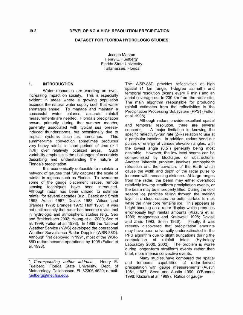
1

J9.2 DEVELOPING A HIGH RESOLUTION PRECIPITATION

DATASET FOR FLORIDA HYDROLOGIC STUDIES

Joseph MarzenHenry E. Fuelberg*

Florida State UniversityTallahassee, Florida

1. INTRODUCTIONWater resources are exerting an ever-

increasing impact on society. This is especiallyevident in areas where a growing populationexceeds the natural water supply such that watershortages ensue. To manage and maintain asuccessful water balance, accurate rainfallmeasurements are needed. Florida’s precipitationoccurs primarily during the summer months,generally associated with typical sea breeze-induced thunderstorms, but occasionally due totropical systems such as hurricanes. Thissummer-time convection sometimes producesvery heavy rainfall in short periods of time (> 1in./h) over relatively localized areas. Suchvariability emphasizes the challenges of accuratelydescribing and understanding the nature ofFlorida’s precipitation.

It is economically unfeasible to maintain anetwork of gauges that fully captures the scale ofrainfall in regions such as Florida. To overcomesome of the gauge placement issues, remotesensing techniques have been introduced.Although radar has been utilized to estimaterainfall for several decades (e.g., Baeck and Smith1998; Austin 1987; Doviak 1983; Wilson andBrandes 1979; Brandes 1975; Huff 1967), it wasnot until recently that radar has become a vital toolin hydrologic and atmospheric studies (e.g., Seoand Breidenbach 2002; Young et al. 2000; Seo etal. 1999; Fulton et al. 1998). In 1988 the NationalWeather Service (NWS) developed the operationalWeather Surveillance Radar Doppler (WSR-88D).Although first deployed in 1991, most of the WSR-88D radars became operational by 1996 (Fulton etal. 1998).

* Corresponding author address: Henry E.Fuelberg, Florida State University, Dept. ofMeteorology, Tallahassee, FL 32306-4520; e-mail:[email protected].

The WSR-88D provides reflectivities at highspatial (1 km range, 1-degree azimuth) andtemporal resolution (scans every 6 min.) and anaerial coverage out to 230 km from the radar site.The main algorithm responsible for producingrainfall estimates from the reflectivities is thePrecipitation Processing Subsystem (PPS) (Fultonet al. 1998).

Although radars provide excellent spatialand temporal resolution, there are severalconcerns. A major limitation is knowing thespecific reflectivity-rain rate (Z-R) relation to use ata particular location. In addition, radars send outpulses of energy at various elevation angles, withthe lowest angle (0.5°) generally being mostdesirable. However, the low level beams can becompromised by blockages or obstructions.Another inherent problem involves atmosphericrefraction and the curvature of the Earth whichcause the width and depth of the radar pulse toincrease with increasing distance. At large rangesfrom the radar, the beam may either overshootrelatively low-top stratiform precipitation events, orthe beam may be improperly filled. During the coldseason ice particles falling through the meltinglayer in a cloud causes the outer surface to meltwhile the inner core remains ice. This appears asbright banding on a radar display which produceserroneously high rainfall amounts (Klazura et al.1999; Anagnostou and Krajewski 1998; Doviakand Zrnic 1993; Smith 1986). Finally, it wasrecently discovered that precipitation amountsmay have been universally underestimated in thePPS algorithm due to slight truncations during thecomputation of rainfall totals (HydrologyLaboratory 2000, 2002). The problem is worseduring longer-term stratiform events rather thanbrief, more intense convective events.

Many studies have compared the spatialand temporal capabilities of radar-derivedprecipitation with gauge measurements (Austin1981, 1987; Seed and Austin 1990; O’Bannon1998; Klazura et al. 1999). Ratios of gauge-

2

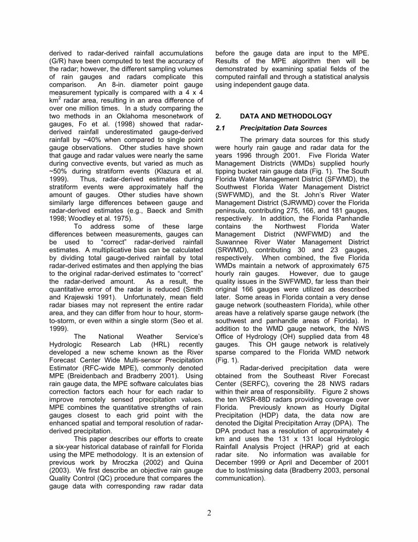
derived to radar-derived rainfall accumulations(G/R) have been computed to test the accuracy ofthe radar; however, the different sampling volumesof rain gauges and radars complicate thiscomparison. An 8-in. diameter point gaugemeasurement typically is compared with a 4 x 4km2 radar area, resulting in an area difference ofover one million times. In a study comparing thetwo methods in an Oklahoma mesonetwork ofgauges, Fo et al. (1998) showed that radar-derived rainfall underestimated gauge-derivedrainfall by ~40% when compared to single pointgauge observations. Other studies have shownthat gauge and radar values were nearly the sameduring convective events, but varied as much as~50% during stratiform events (Klazura et al.1999). Thus, radar-derived estimates duringstratiform events were approximately half theamount of gauges. Other studies have shownsimilarly large differences between gauge andradar-derived estimates (e.g., Baeck and Smith1998; Woodley et al. 1975).

To address some of these largedifferences between measurements, gauges canbe used to “correct” radar-derived rainfallestimates. A multiplicative bias can be calculatedby dividing total gauge-derived rainfall by totalradar-derived estimates and then applying the biasto the original radar-derived estimates to “correct”the radar-derived amount. As a result, thequantitative error of the radar is reduced (Smithand Krajewski 1991). Unfortunately, mean fieldradar biases may not represent the entire radararea, and they can differ from hour to hour, storm-to-storm, or even within a single storm (Seo et al.1999).

The National Weather Service’sHydrologic Research Lab (HRL) recentlydeveloped a new scheme known as the RiverForecast Center Wide Multi-sensor PrecipitationEstimator (RFC-wide MPE), commonly denotedMPE (Breidenbach and Bradberry 2001). Usingrain gauge data, the MPE software calculates biascorrection factors each hour for each radar toimprove remotely sensed precipitation values.MPE combines the quantitative strengths of raingauges closest to each grid point with theenhanced spatial and temporal resolution of radar-derived precipitation.

This paper describes our efforts to createa six-year historical database of rainfall for Floridausing the MPE methodology. It is an extension ofprevious work by Mroczka (2002) and Quina(2003). We first describe an objective rain gaugeQuality Control (QC) procedure that compares thegauge data with corresponding raw radar data

before the gauge data are input to the MPE.Results of the MPE algorithm then will bedemonstrated by examining spatial fields of thecomputed rainfall and through a statistical analysisusing independent gauge data.

2. DATA AND METHODOLOGY2.1 Precipitation Data Sources

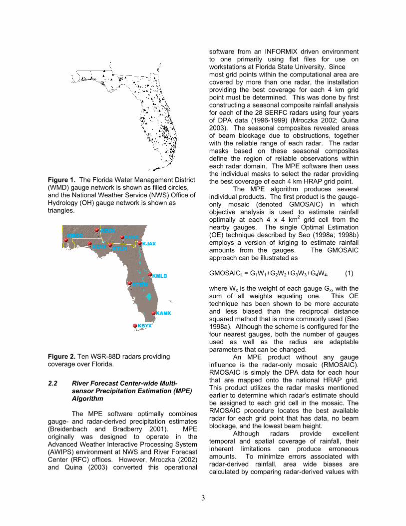
The primary data sources for this studywere hourly rain gauge and radar data for theyears 1996 through 2001. Five Florida WaterManagement Districts (WMDs) supplied hourlytipping bucket rain gauge data (Fig. 1). The SouthFlorida Water Management District (SFWMD), theSouthwest Florida Water Management District(SWFWMD), and the St. John’s River WaterManagement District (SJRWMD) cover the Floridapeninsula, contributing 275, 166, and 181 gauges,respectively. In addition, the Florida Panhandlecontains the Northwest Florida WaterManagement District (NWFWMD) and theSuwannee River Water Management District(SRWMD), contributing 30 and 23 gauges,respectively. When combined, the five FloridaWMDs maintain a network of approximately 675hourly rain gauges. However, due to gaugequality issues in the SWFWMD, far less than theiroriginal 166 gauges were utilized as describedlater. Some areas in Florida contain a very densegauge network (southeastern Florida), while otherareas have a relatively sparse gauge network (thesouthwest and panhandle areas of Florida). Inaddition to the WMD gauge network, the NWSOffice of Hydrology (OH) supplied data from 48gauges. This OH gauge network is relativelysparse compared to the Florida WMD network(Fig. 1).

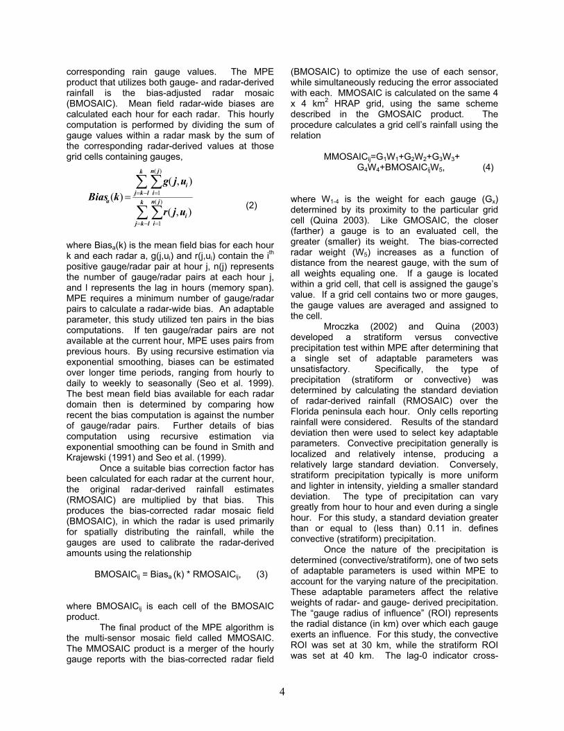
Radar-derived precipitation data wereobtained from the Southeast River ForecastCenter (SERFC), covering the 28 NWS radarswithin their area of responsibility. Figure 2 showsthe ten WSR-88D radars providing coverage overFlorida. Previously known as Hourly DigitalPrecipitation (HDP) data, the data now aredenoted the Digital Precipitation Array (DPA). TheDPA product has a resolution of approximately 4km and uses the 131 x 131 local HydrologicRainfall Analysis Project (HRAP) grid at eachradar site. No information was available forDecember 1999 or April and December of 2001due to lost/missing data (Bradberry 2003, personalcommunication).

3

Figure 1. The Florida Water Management District(WMD) gauge network is shown as filled circles,and the National Weather Service (NWS) Office ofHydrology (OH) gauge network is shown astriangles.

Figure 2. Ten WSR-88D radars providingcoverage over Florida.

2.2 River Forecast Center-wide Multi-sensor Precipitation Estimation (MPE)Algorithm

The MPE software optimally combinesgauge- and radar-derived precipitation estimates(Breidenbach and Bradberry 2001). MPEoriginally was designed to operate in theAdvanced Weather Interactive Processing System(AWIPS) environment at NWS and River ForecastCenter (RFC) offices. However, Mroczka (2002)and Quina (2003) converted this operational

software from an INFORMIX driven environmentto one primarily using flat files for use onworkstations at Florida State University. Sincemost grid points within the computational area arecovered by more than one radar, the installationproviding the best coverage for each 4 km gridpoint must be determined. This was done by firstconstructing a seasonal composite rainfall analysisfor each of the 28 SERFC radars using four yearsof DPA data (1996-1999) (Mroczka 2002; Quina2003). The seasonal composites revealed areasof beam blockage due to obstructions, togetherwith the reliable range of each radar. The radarmasks based on these seasonal compositesdefine the region of reliable observations withineach radar domain. The MPE software then usesthe individual masks to select the radar providingthe best coverage of each 4 km HRAP grid point.

The MPE algorithm produces severalindividual products. The first product is the gauge-only mosaic (denoted GMOSAIC) in whichobjective analysis is used to estimate rainfalloptimally at each 4 x 4 km2 grid cell from thenearby gauges. The single Optimal Estimation(OE) technique described by Seo (1998a; 1998b)employs a version of kriging to estimate rainfallamounts from the gauges. The GMOSAICapproach can be illustrated as

GMOSAICij = G1W1+G2W2+G3W3+G4W4, (1)

where Wx is the weight of each gauge Gx, with thesum of all weights equaling one. This OEtechnique has been shown to be more accurateand less biased than the reciprocal distancesquared method that is more commonly used (Seo1998a). Although the scheme is configured for thefour nearest gauges, both the number of gaugesused as well as the radius are adaptableparameters that can be changed.

An MPE product without any gaugeinfluence is the radar-only mosaic (RMOSAIC).RMOSAIC is simply the DPA data for each hourthat are mapped onto the national HRAP grid.This product utilizes the radar masks mentionedearlier to determine which radar’s estimate shouldbe assigned to each grid cell in the mosaic. TheRMOSAIC procedure locates the best availableradar for each grid point that has data, no beamblockage, and the lowest beam height.

Although radars provide excellenttemporal and spatial coverage of rainfall, theirinherent limitations can produce erroneousamounts. To minimize errors associated withradar-derived rainfall, area wide biases arecalculated by comparing radar-derived values with

4

corresponding rain gauge values. The MPEproduct that utilizes both gauge- and radar-derivedrainfall is the bias-adjusted radar mosaic(BMOSAIC). Mean field radar-wide biases arecalculated each hour for each radar. This hourlycomputation is performed by dividing the sum ofgauge values within a radar mask by the sum ofthe corresponding radar-derived values at thosegrid cells containing gauges,

where Biasa(k) is the mean field bias for each hourk and each radar a, g(j,ui) and r(j,ui) contain the ithpositive gauge/radar pair at hour j, n(j) representsthe number of gauge/radar pairs at each hour j,and l represents the lag in hours (memory span).MPE requires a minimum number of gauge/radarpairs to calculate a radar-wide bias. An adaptableparameter, this study utilized ten pairs in the biascomputations. If ten gauge/radar pairs are notavailable at the current hour, MPE uses pairs fromprevious hours. By using recursive estimation viaexponential smoothing, biases can be estimatedover longer time periods, ranging from hourly todaily to weekly to seasonally (Seo et al. 1999).The best mean field bias available for each radardomain then is determined by comparing howrecent the bias computation is against the numberof gauge/radar pairs. Further details of biascomputation using recursive estimation viaexponential smoothing can be found in Smith andKrajewski (1991) and Seo et al. (1999).

Once a suitable bias correction factor hasbeen calculated for each radar at the current hour,the original radar-derived rainfall estimates(RMOSAIC) are multiplied by that bias. Thisproduces the bias-corrected radar mosaic field(BMOSAIC), in which the radar is used primarilyfor spatially distributing the rainfall, while thegauges are used to calibrate the radar-derivedamounts using the relationship

BMOSAICij = Biasa (k) * RMOSAICij, (3)

where BMOSAICij is each cell of the BMOSAICproduct.

The final product of the MPE algorithm isthe multi-sensor mosaic field called MMOSAIC.The MMOSAIC product is a merger of the hourlygauge reports with the bias-corrected radar field

(BMOSAIC) to optimize the use of each sensor,while simultaneously reducing the error associatedwith each. MMOSAIC is calculated on the same 4x 4 km2 HRAP grid, using the same schemedescribed in the GMOSAIC product. Theprocedure calculates a grid cell’s rainfall using therelation

MMOSAICij=G1W1+G2W2+G3W3+G4W4+BMOSAICijW5, (4)

where W1-4 is the weight for each gauge (Gx)determined by its proximity to the particular gridcell (Quina 2003). Like GMOSAIC, the closer(farther) a gauge is to an evaluated cell, thegreater (smaller) its weight. The bias-correctedradar weight (W5) increases as a function ofdistance from the nearest gauge, with the sum ofall weights equaling one. If a gauge is locatedwithin a grid cell, that cell is assigned the gauge’svalue. If a grid cell contains two or more gauges,the gauge values are averaged and assigned tothe cell.

Mroczka (2002) and Quina (2003)developed a stratiform versus convectiveprecipitation test within MPE after determining thata single set of adaptable parameters wasunsatisfactory. Specifically, the type ofprecipitation (stratiform or convective) wasdetermined by calculating the standard deviationof radar-derived rainfall (RMOSAIC) over theFlorida peninsula each hour. Only cells reportingrainfall were considered. Results of the standarddeviation then were used to select key adaptableparameters. Convective precipitation generally islocalized and relatively intense, producing arelatively large standard deviation. Conversely,stratiform precipitation typically is more uniformand lighter in intensity, yielding a smaller standarddeviation. The type of precipitation can varygreatly from hour to hour and even during a singlehour. For this study, a standard deviation greaterthan or equal to (less than) 0.11 in. definesconvective (stratiform) precipitation.

Once the nature of the precipitation isdetermined (convective/stratiform), one of two setsof adaptable parameters is used within MPE toaccount for the varying nature of the precipitation.These adaptable parameters affect the relativeweights of radar- and gauge- derived precipitation.The “gauge radius of influence” (ROI) representsthe radial distance (in km) over which each gaugeexerts an influence. For this study, the convectiveROI was set at 30 km, while the stratiform ROIwas set at 40 km. The lag-0 indicator cross-

(2)∑∑

∑∑

−= =

−= == k

lkj

jn

ii

k

lkj

jn

ii

a

ujr

ujgkBias )(

1

)(

1

),(

),()(

,

5

correlation and the lag-0 conditional crosscorrelation parameters are used to assign relativeweights to gauges and radars (Breidenbach andBradberry 2001). Both of these correlationparameters can range from zero to one, with zeroyielding the GMOSAIC product, and oneproducing the BMOSAIC product. Hence, greatercorrelation values produce a greater influence byBMOSAIC, while smaller values yield a greaterinfluence from the gauges. Since convective(stratiform) rainfall events generally are heavy(light) and spotty (uniform), more weight should begiven to BMOSAIC (GMOSAIC). Following thismethodology, both correlation parameters wereset at 0.925 for convective precipitation and to0.65 for stratiform precipitation. Various sensitivitytests of these parameters showed the valueschosen to be most optimal for the Floridapeninsula (Quina 2003).

3. RAIN GAUGE QUALITY CONTROL3.1 Problems Encountered

We utilized rain gauge data from all fiveFlorida’s WMDs, together with a supplementaldataset provided by the NWS OH, a total of over700 gauges (Fig. 1). A detailed inspection of theoriginal gauge data showed varying degrees ofquality.

The SFWMD provided 275 operationalgauges for this study. The SFWMD hadperformed its own quality control check on theirdata. Hourly rain gauge values were assignedone of several different quality control (QC)indicators to document the resulting output of theirprocedure.

The SRWMD supplied 23 gauges,comprising a relatively sparse network and notcovering the entire study period. In fact, gaugedata were supplied only for the years 1998through 2001, with only minimal useable dataduring 1998 and 1999. There was nodocumentation of a QC procedure having beenapplied to the data. A major quality control issuewas discovered regarding the timing of theSRWMD data. Specifically, the time attributed to agauge observation often did not agree with theradar-observed timing (i.e., they seemed to differby plus or minus one hour). This timing problemdid not appear with all gauges and did not appearto span the entire period of record. However, nospecific documentation about these problematicgauges was provided. Therefore, the data had to

be examined carefully to identify those gaugeshaving the timing problem and to determine thetime periods over which they occurred.

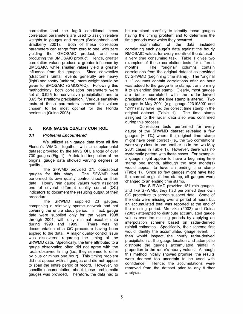
Examination of the data includedcorrelating each gauge’s data against the hourlyRMOSAIC values for every month of the dataset--a very time consuming task. Table 1 gives twoexamples of these correlation tests for differentmonths. The “original” columns containcorrelations from the original dataset as providedby SRWMD (beginning time stamp). The “original+ 1” columns contain correlations after an hourwas added to the gauge time stamp, transformingit to an ending time stamp. Clearly, most gaugesare better correlated with the radar-derivedprecipitation when the time stamp is altered. Twogauges in May 2001 (e.g., gauge “2319800” and“241”) may have had the correct time stamp in theoriginal dataset (Table 1). The time stampassigned to the radar data also was confirmedduring this process.

Correlation tests performed for everygauge of the SRWMD dataset revealed a fewgauges (~ 1%) where the original time stampmight have been correct (i.e., the two correlationswere very close to one another as in the two May2001 cases in Table 1). However, there was nosystematic pattern with these cases. For example,a gauge might appear to have a beginning timestamp one month, although the next month(s)would appear to have an ending time stamp(Table 1). Since so few gauges might have hadthe correct original time stamp, all gauges werechanged to an ending time stamp.

The SJRWMD provided 181 rain gauges,and like SFWMD, they had performed their ownQC procedure to screen suspect data. Some ofthe data were missing over a period of hours butan accumulated total was reported at the end ofthe missing period. Mroczka (2002) and Quina(2003) attempted to distribute accumulated gaugevalues over the missing periods by applying aninterpolation scheme based on radar-derivedrainfall estimates. Specifically, their scheme firstwould identify the accumulated gauge event. Itthen would inspect the hourly radar-derivedprecipitation at the gauge location and attempt todistribute the gauge’s accumulated rainfall inproportion to the radar’s hourly values. Althoughthis method initially showed promise, the resultswere deemed too uncertain to be used withconfidence. Hence, the accumulations wereremoved from the dataset prior to any furtheranalysis.

6

Table 1. Individual SRWMD gauge correlations with the RMOSAIC radar product for May and August2001.

May 2001 August 2001

Gauge ID Original (Beg. Time)

Original + 1(End Time)

Original (Beg. Time)

Original + 1(End Time)

2319800 0.571 0.509 0.247 0.7362320500 0.090 0.982 0.375 0.6042321500 0.059 0.794 0.256 0.8292323500 0.222 0.899 0.279 0.715

210 0.157 0.647 0.161 0.419229 0.110 0.541 0.050 0.384235 -0.003 0.626 0.084 0.968240 0.191 0.722 0.143 0.884241 0.743 0.508 0.129 0.808246 0.542 0.637 0.288 0.728252 0.234 0.715 0.073 0.719254 0.024 0.840 0.045 0.569263 0.135 0.445 0.180 0.715270 0.042 0.729 0.197 0.829287 0.427 0.932 0.148 0.635

Averages 0.236 0.702 0.177 0.703

Another issue with the SJRWMD data waswhether the proper time stamp had been assignedto the hourly gauge amounts, as described earlierfor the SRWMD data. Therefore, the SJRWMDgauges were correlated with radar data in anattempt to verify the time stamp (as in Table 1).The tests revealed the time stamp to be thebeginning of the collection hour for all gauges.

The NWFWMD provided 30 gaugesspanning the Florida panhandle. The District hadnot applied QC procedures to their data, andseveral major formatting issues needed to beaddressed. MPE requires hourly rain gaugeamounts for effective use; however, much of theNWFWMD data were provided in sub-hourlyincrements. That is, the data were recorded at 5-10- 15- 30- or 60-min time intervals. AlthoughNWFWMD personnel provided a detailed listing ofgauges and their respective data intervalrecordings, many problems still existed. Forexample, some gauges that were specified tocontain only 5-min data increments actually hadother data intervals intertwined within the 5-minincrements (i.e., 15-min summations for somehours, but 5-min for most others). Since thisappeared to occur randomly, substantial effort wasspent identifying the different situations for eachgauge and correcting them by calculating hourlyaccumulations.

The SWFWMD provided 166 gauges overthe western portions of the Florida peninsula.These data have high spatial resolution, similar tothe SFWMD and SJRWMD. However, initialexamination of the SWFWMD gauge datasetshowed a large number of gauges reporting with anon-hourly time stamp, with most in the form of 12h accumulations. There also was a large numberof cases in which the data contained a time stampgreater than or less than one hour. Segregatingthe 12 h accumulations into hourly amounts wouldhave yielded significant uncertainty. Hence, the12-hourly gauges were removed from the dataset.It should be noted that at one time or another, allof the SWFWMD gauges reported some non-hourly amounts, but only those particular hourswere removed. Thus, only those gauges thatreported hourly remained. This initial QC stepremoved 79 gauges from the original 166 thatwere provided, leaving 88 gauges to be examinedfurther. Additional problems with these data aredescribed in a later section.

The NWS OH gauge network wasrelatively sparse compared with the Florida WMDnetwork. These data had been quality controlledby the NWS. Analysis of the OH data revealed thatabout 85% of the gauges reported at a resolutionof only 0.1 in. (not 0.01 in.). Not only was theresolution to the nearest 0.1 in., but the hourly

7

amounts also were truncated. For example, if agauge reporting to the nearest 0.1 in. actuallyreceived 0.09 in. of rain during an hour, a value ofzero would be reported that hour. Unlessadditional rainfall occurred prior to the end of theday, no rain would be recorded that day (Tollerud2000).

3.2 Florida State’s Quality ControlProcedures

A detailed examination of the WMD and

OH gauge data showed that an additional,substantial quality control effort still was neededsince manual inspection revealed many cases ofunusual and unacceptable amounts. An objectiveQC procedure would be required due to largeamount of gauge over the multi-year period.

In attempting to devise an appropriate QCprocedure, there were many discussions withpersonnel at the NWS OH. Several of theirprocedures were investigated but found to beunsatisfactory for our use. For example, a “buddycheck” procedure was attempted. However, sinceFlorida’s rainfall is very localized, many valueswere flagged as being suspicious when theyactually appeared quite reasonable. A temporalconsistency check procedure was investigated toidentify “stuck” rain gauges (zero values occurringduring rainfall). After individually summing dailygauge and radar rainfall values, differencesbetween the two are checked against a set ofcriteria. This technique also providedunacceptable results, again due to the highlyvariable nature of Florida rainfall.

Another attempt at quality controlling raingauge data was to plot gauge data ontocorresponding radar imagery (RMOSAIC). Basedon several test cases of this method, it was soonabandoned since it was deemed too subjectiveand too time intensive because every hourrequired manual inspection.

We developed a QC procedure thatobjectively compared hourly gauge values withraw radar-derived values (i.e., RMOSAIC beforeany modifications). Specifically, each hourlygauge value was compared to the 4 x 4 km2 radar-derived estimate whose area contained the gauge.This proved to be a fruitful approach since thegauge data were objectively compared with anindependent source (the radar) and since the high-resolution radar data are more likely to detectFlorida’s spotty rainfall patterns than the gaugenetworks (e.g., the “buddy check” procedure). Tothe authors’ knowledge, this type of objectiveevaluation of gauge data against radar values has

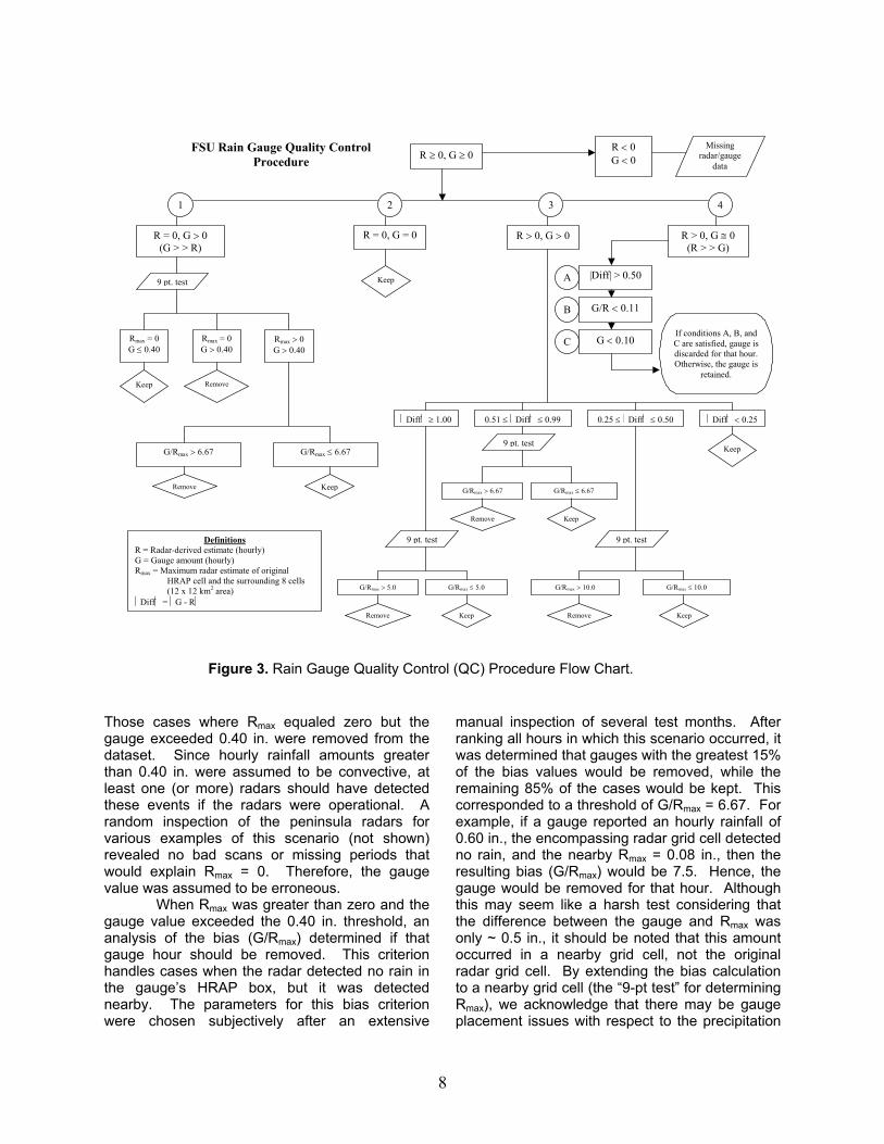
not been reported previously. Figure 3 is a flowchart of this scheme, and the following sectionsdetail the various steps of the procedure alongwith justifications for choosing some of theadaptable parameters that are contained within.We state at the outset that there is no perfectscheme for quality controlling precipitation data.

Since gauge and radar precipitationvalues must be positive, any hours with missingdata were immediately removed from the dataset.Hence, only hours with both gauge amounts (G)and radar-derived estimates (R) greater than orequal to zero were passed through the procedure.The remaining non-zero data then were evaluatedagainst four additional criteria that are discussedindividually below (numbered at the top of Fig. 3).

1) R = 0, G > 0 ConditionStep 1 of the QC procedure (Fig. 3)

evaluated hours when the gauge reported rainfall,but the radar did not. If a gauge reported rainfall,but the encompassing 4 x 4 km2 radar grid cellexhibited no rain, the radar area around the gaugewas expanded to include the eight surroundingHRAP grid boxes (12 x 12 km2). This criterionhereafter will be denoted the “9-pt. test”, while themaximum radar-derived estimate within the ninegrid boxes will be denoted “Rmax”. This expansionin the test area was designed to consider caseswhen a gauge was located at the boundary of anHRAP grid cell and that gauge marked the edge ofthe precipitation area. When the gauge reportedrainfall, but all nine radar values indicated zerorainfall (Rmax = 0.00 in.), a sliding scale wasestablished to determine whether the gauge valuewas acceptable. A gauge threshold wasdetermined for comparison with the surroundingradar pixels (12 x 12 km2). Specifically, the hourlygauge value was kept when its value was lessthan or equal to 0.40 in. of rain (an adaptableparameter), even though R and Rmax equaled zero.We hypothesized that rainfall exceeding 0.40 in. inan hour likely was convective. Therefore, theradar should detect this rainfall since convectiveclouds generally extend relatively high in theatmosphere (Baeck and Smith 1998). Conversely,if an hourly gauge value was less than 0.40 in., theprecipitation more likely was stratiform incharacter, and the radar beam could overshoot therelatively low echo tops, giving a zero value. Dueto the potential for considerable uncertainty incomparing a point gauge value to a radar-derived4 x 4 km2 area, the 0.40 in. minimum gaugethreshold was chosen rather generously.

8

Figure 3. Rain Gauge Quality Control (QC) Procedure Flow Chart.

Those cases where Rmax equaled zero but thegauge exceeded 0.40 in. were removed from thedataset. Since hourly rainfall amounts greaterthan 0.40 in. were assumed to be convective, atleast one (or more) radars should have detectedthese events if the radars were operational. Arandom inspection of the peninsula radars forvarious examples of this scenario (not shown)revealed no bad scans or missing periods thatwould explain Rmax = 0. Therefore, the gaugevalue was assumed to be erroneous.

When Rmax was greater than zero and thegauge value exceeded the 0.40 in. threshold, ananalysis of the bias (G/Rmax) determined if thatgauge hour should be removed. This criterionhandles cases when the radar detected no rain inthe gauge’s HRAP box, but it was detectednearby. The parameters for this bias criterionwere chosen subjectively after an extensive

manual inspection of several test months. Afterranking all hours in which this scenario occurred, itwas determined that gauges with the greatest 15%of the bias values would be removed, while theremaining 85% of the cases would be kept. Thiscorresponded to a threshold of G/Rmax = 6.67. Forexample, if a gauge reported an hourly rainfall of0.60 in., the encompassing radar grid cell detectedno rain, and the nearby Rmax = 0.08 in., then theresulting bias (G/Rmax) would be 7.5. Hence, thegauge would be removed for that hour. Althoughthis may seem like a harsh test considering thatthe difference between the gauge and Rmax wasonly ~ 0.5 in., it should be noted that this amountoccurred in a nearby grid cell, not the originalradar grid cell. By extending the bias calculationto a nearby grid cell (the “9-pt test” for determiningRmax), we acknowledge that there may be gaugeplacement issues with respect to the precipitation

R ≥ 0, G ≥ 0R < 0 G < 0

R = 0, G > 0 (G > > R)

R = 0, G = 0 R > 0, G > 0

9 pt. test

1 2

Rmax = 0 G ≤ 0.40

Rmax = 0 G > 0.40

Rmax > 0 G > 0.40

Keep

G/Rmax > 6.67 G/Rmax ≤ 6.67

Keep

Diff < 0.250.25 ≤ Diff ≤ 0.50 0.51 ≤ Diff ≤ 0.99Diff ≥ 1.00

Keep

9 pt. test

9 pt. test

9 pt. test

G/Rmax ≤ 5.0 G/Rmax > 5.0

KeepRemove

G/Rmax > 6.67

KeepRemove

G/Rmax ≤ 6.67

G/Rmax > 10.0 G/Rmax ≤ 10.0

Remove Keep

C

B

AKeep

Remove

Remove

3 4

R > 0, G ≅ 0 (R > > G)

Missing radar/gauge

data

G/R < 0.11

G < 0.10 If conditions A, B, and C are satisfied, gauge is discarded for that hour. Otherwise, the gauge is

retained.

FSU Rain Gauge Quality Control Procedure

Definitions R = Radar-derived estimate (hourly) G = Gauge amount (hourly) Rmax = Maximum radar estimate of original

HRAP cell and the surrounding 8 cells (12 x 12 km2 area)

Diff = G - R

|Diff| > 0.50

9

and that the precipitation likely is moving overdifferent grid cells. This prevents the gauge frommistakenly being removed because the originalradar grid cell detected nothing; whereasprecipitation did in fact, occur nearby.

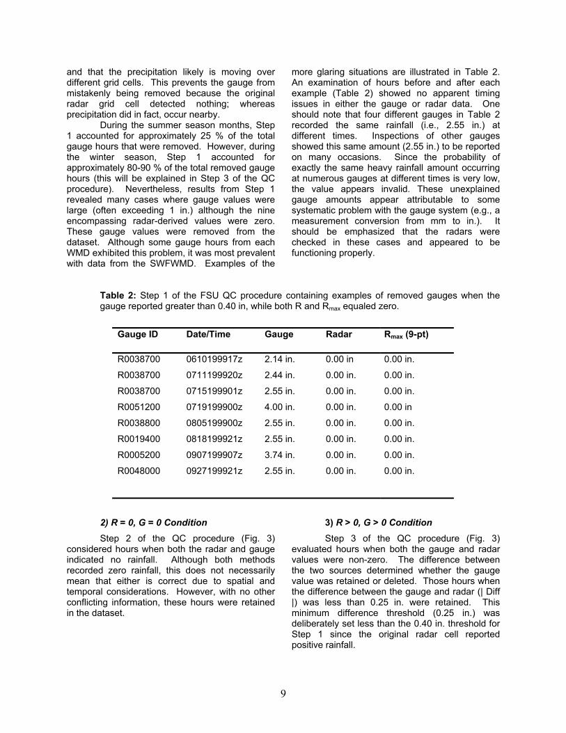
During the summer season months, Step1 accounted for approximately 25 % of the totalgauge hours that were removed. However, duringthe winter season, Step 1 accounted forapproximately 80-90 % of the total removed gaugehours (this will be explained in Step 3 of the QCprocedure). Nevertheless, results from Step 1revealed many cases where gauge values werelarge (often exceeding 1 in.) although the nineencompassing radar-derived values were zero.These gauge values were removed from thedataset. Although some gauge hours from eachWMD exhibited this problem, it was most prevalentwith data from the SWFWMD. Examples of the

more glaring situations are illustrated in Table 2.An examination of hours before and after eachexample (Table 2) showed no apparent timingissues in either the gauge or radar data. Oneshould note that four different gauges in Table 2recorded the same rainfall (i.e., 2.55 in.) atdifferent times. Inspections of other gaugesshowed this same amount (2.55 in.) to be reportedon many occasions. Since the probability ofexactly the same heavy rainfall amount occurringat numerous gauges at different times is very low,the value appears invalid. These unexplainedgauge amounts appear attributable to somesystematic problem with the gauge system (e.g., ameasurement conversion from mm to in.). Itshould be emphasized that the radars werechecked in these cases and appeared to befunctioning properly.

Table 2: Step 1 of the FSU QC procedure containing examples of removed gauges when thegauge reported greater than 0.40 in, while both R and Rmax equaled zero.

Gauge ID Date/Time Gauge Radar Rmax (9-pt)

R0038700 0610199917z 2.14 in. 0.00 in 0.00 in.

R0038700 0711199920z 2.44 in. 0.00 in. 0.00 in.

R0038700 0715199901z 2.55 in. 0.00 in. 0.00 in.

R0051200 0719199900z 4.00 in. 0.00 in. 0.00 in

R0038800 0805199900z 2.55 in. 0.00 in. 0.00 in.

R0019400 0818199921z 2.55 in. 0.00 in. 0.00 in.

R0005200 0907199907z 3.74 in. 0.00 in. 0.00 in.

R0048000 0927199921z 2.55 in. 0.00 in. 0.00 in.

2) R = 0, G = 0 ConditionStep 2 of the QC procedure (Fig. 3)

considered hours when both the radar and gaugeindicated no rainfall. Although both methodsrecorded zero rainfall, this does not necessarilymean that either is correct due to spatial andtemporal considerations. However, with no otherconflicting information, these hours were retainedin the dataset.

3) R > 0, G > 0 ConditionStep 3 of the QC procedure (Fig. 3)

evaluated hours when both the gauge and radarvalues were non-zero. The difference betweenthe two sources determined whether the gaugevalue was retained or deleted. Those hours whenthe difference between the gauge and radar (| Diff|) was less than 0.25 in. were retained. Thisminimum difference threshold (0.25 in.) wasdeliberately set less than the 0.40 in. threshold forStep 1 since the original radar cell reportedpositive rainfall.

10

Differences between radar and gaugeamounts greater than the 0.25 in. threshold wereseparated into three additional categories (Fig. 3):1) between 0.25 in. and 0.50 in., 2) between 0.51in. and 0.99 in., and 3) greater than or equal to1.00 in. In each case, the gauge valuesunderwent the 9-pt test and were classified aseither good or bad according to the additional biascriterion check (G/Rmax) described earlier. Thebias threshold parameters again were chosensubjectively after manual inspections of the datarevealed the appropriate acceptable andunacceptable differences between gauge andradar amounts.

For gauge and radar differences less thanor equal to 0.50 in. but greater than or equal to0.25 in., only the gauges with the largest biaseswere removed. As described earlier for Step 1,extending the bias to include the nearby radar gridcells accounts for gauge location with respect tothe precipitation, in addition to movingprecipitation. Since both the gauge and radarreported rainfall, only those situations with thegreatest 10% of the bias values based on all ninegrid boxes were removed (G/Rmax > 10.0). Forexample, if a gauge reported 0.55 in. and theradar reported 0.03 in. of rainfall in an hour, theminimum acceptable radar amount in the nine gridcells (Rmax) would be 0.05 in. (G/Rmax = 11). IfRmax = 0.04 in. in this case (G/Rmax = 13.75), thegauge hour would be removed. Inspections ofthese scenarios revealed that the nearby radar

grid cells generally had a greater rainfall than thegauge’s grid cell. Therefore, Rmax would begreater than R, the bias would meet theacceptable criterion, and the gauge would be kept.Very few gauge hours were removed due to thiscriterion.

When the gauge and radar difference wasbetween 0.51 in. and 0.99 in (or > 1.00 in.), thesame methodology was applied. After the 9-pttest, a gauge was removed when the bias (G/Rmax)criterion exceeded 6.67 (5.0). This valuecorresponds to the greatest 15% (20%) of thebiases. The remaining 85% (80%) of the caseswere kept. We decreased the percentage biascriterion for the larger gauge-radar differencesbetween a gauge and radar (> 1.00 in.) to includea larger range of suspect data. For example, if thegauge reported 2.30 in. of rainfall in an hour, andthe radar reported 0.40 in., the minimumacceptable radar amount in the nine grid cellswould be 0.46 in. If Rmax = 0.45 in. in this case,that gauge hour would be removed.

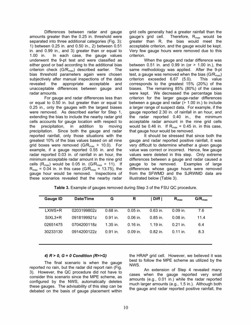
It should be stressed that since both thegauge and radar reported positive rainfall, it wasvery difficult to determine whether a given gaugevalue was correct or incorrect. Hence, few gaugevalues were deleted in this step. Only extremedifferences between a gauge and radar caused agauge to be removed. Examples of largedifferences whose gauge hours were removedfrom the SFWMD and the SJRWMD data areillustrated below (Table 3).

Table 3. Example of gauges removed during Step 3 of the FSU QC procedure.

Gauge ID Date/Time G R | Diff | Rmax G/Rmax

LXWS+R 0203199802z 0.68 in. 0.05 in. 0.63 in. 0.09 in. 7.6

SIXL3+R 0918199921z 0.91 in. 0.06 in. 0.85 in. 0.08 in. 11.4

02651475 0704200118z 1.35 in. 0.16 in. 1.19 in. 0.21 in. 6.4

30233130 0914200122z 0.91 in. 0.09 in. 0.82 in. 0.11 in. 8.3

4) R > 0, G = 0 Condition (R>>G)The final scenario is when the gauge

reported no rain, but the radar did report rain (Fig.3). However, the QC procedure did not have toconsider this scenario since the MPE scheme, asconfigured by the NWS, automatically deletesthese gauges. The advisability of this step can bedebated on the basis of gauge placement within

the HRAP grid cell. However, we believed it wasbest to follow the MPE scheme as utilized by theNWS.

An extension of Step 4 revealed manycases when the gauge reported very smallamounts (e.g., 0.01 in.) while the radar reportedmuch larger amounts (e.g., 1.5 in.). Although boththe gauge and radar reported positive rainfall, the

11

gauge values appeared unrepresentative of thearea-wide rainfall. Thus, three additional criteriawere established to determine whether the gaugeshould be removed from the dataset. Theconditions establishing removal were: 1) thedifference between the gauge and radar amountsmust be greater than or equal 0.51 in. (Condition Ain Fig. 3); 2) the bias between the gauge valueand the encompassing radar (G/R) value must beless than 0.11 (Condition B), and 3) the gaugevalue must be less than 0.10 in (Condition C).Since gauge placement issues within a 4 x 4 km2

grid cell could account for such large differences,gauges only were discarded if all three conditionswere satisfied that particular hour. These criteriawere chosen subjectively after extensive testing ofthese cases. By establishing the three additional

conditions for this situation, we believe weremoved the most suspect gauge data, whilepreserving most of the representative cases.

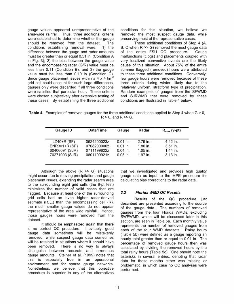
These additional conditions of Step 4 (A,B, C when R >> G) removed the most gauge dataof the entire FSU QC procedure. Gaugemalfunctions (clogs) and placements coupled withvery localized convective events are the likelycause of this situation. About 75% of the entiresummer flagged (removed) hours were attributedto these three additional conditions. Conversely,few gauge hours were removed because of thesethree criteria during winter, likely due to therelatively uniform, stratiform type of precipitation.Random examples of gauges from the SFWMDand SJRWMD that were removed by theseconditions are illustrated in Table 4 below.

Table 4. Examples of removed gauges for the three additional conditions applied to Step 4 when G > 0,R > 0, and R >> G.

Gauge ID Date/Time Gauge Radar Rmax (9-pt)

LZ40+R (SF) 0624200023z 0.01 in. 2.79 in. 4.42 in.ENR301+R (SF) 0708200000z 0.01 in. 1.86 in. 3.51 in.60406091 (SJR) 0711199822z 0.04 in. 1.05 in. 1.44 in.70271003 (SJR) 0801199921z 0.05 in. 1.97 in. 3.13 in.

Although the above (R >> G) situationsmight occur due to moving precipitation and gaugeplacement issues, extending the radar search areato the surrounding eight grid cells (the 9-pt test)minimizes the number of valid cases that areflagged. Because at least one of the surroundinggrid cells had an even higher radar-derivedestimate (Rmax) than the encompassing cell (R),the much smaller gauge values do not appearrepresentative of the area wide rainfall. Hence,those gauges hours were removed from thedataset.

It should be emphasized again that thereis no perfect QC procedure. Inevitably, goodgauge data sometimes will be mistakenlyremoved, while suspect gauge data sometimeswill be retained in situations where it should havebeen removed. There is no way to alwaysdistinguish between accurate and erroneousgauge amounts. Steiner et al. (1999) notes thatthis is especially true in an operationalenvironment and for sparse gauge networks.Nonetheless, we believe that this objectiveprocedure is superior to any of the alternatives

that we investigated and provides high qualitygauge data as input to the MPE procedure forcalculating bias corrections to the radar data.

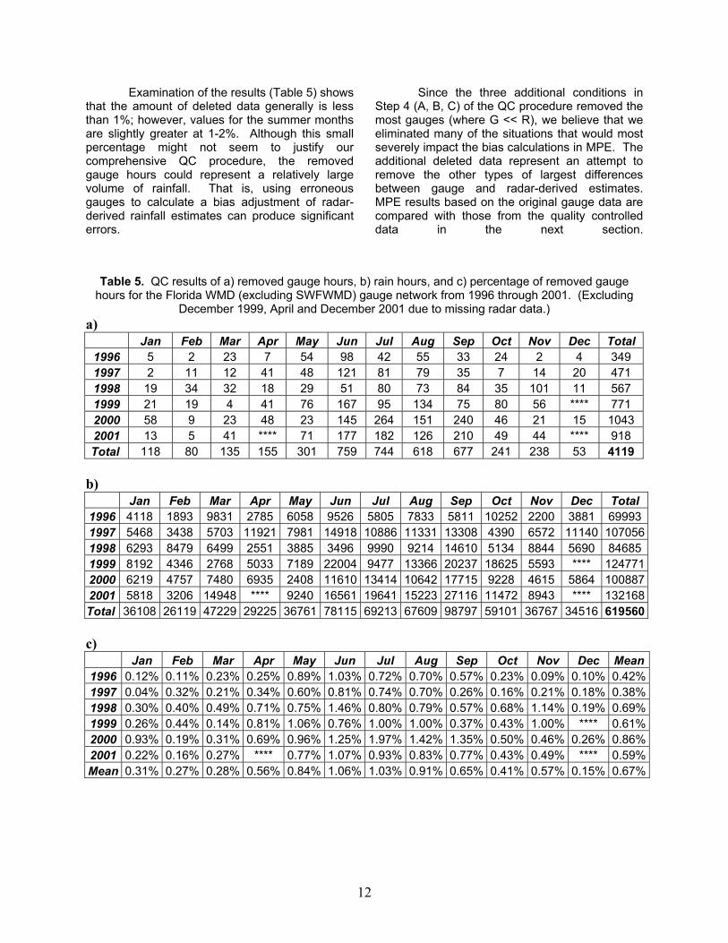
3.3 Florida WMD QC ResultsResults of the QC procedure just

described are presented according to the sourceof the gauge data. The numbers of removedgauges from the four Florida WMDs, excludingSWFWMD, which will be discussed later in thissection, are seen in Table 5a. Each monthly valuerepresents the number of removed gauges fromeach of the four WMD datasets. Rainy hours(Table 5b) were defined as a gauge reporting anhourly total greater than or equal to 0.01 in. Thepercentage of removed gauge hours then wascalculated by dividing the removed hours by thetotal rainy hours (Table 5c). One should note theasterisks in several entries, denoting that radardata for these months either was missing orproblematic, in which case no QC analyses wereperformed.

12

Examination of the results (Table 5) showsthat the amount of deleted data generally is lessthan 1%; however, values for the summer monthsare slightly greater at 1-2%. Although this smallpercentage might not seem to justify ourcomprehensive QC procedure, the removedgauge hours could represent a relatively largevolume of rainfall. That is, using erroneousgauges to calculate a bias adjustment of radar-derived rainfall estimates can produce significanterrors.

Since the three additional conditions inStep 4 (A, B, C) of the QC procedure removed themost gauges (where G << R), we believe that weeliminated many of the situations that would mostseverely impact the bias calculations in MPE. Theadditional deleted data represent an attempt toremove the other types of largest differencesbetween gauge and radar-derived estimates.MPE results based on the original gauge data arecompared with those from the quality controlleddata in the next section.

Table 5. QC results of a) removed gauge hours, b) rain hours, and c) percentage of removed gaugehours for the Florida WMD (excluding SWFWMD) gauge network from 1996 through 2001. (Excluding

December 1999, April and December 2001 due to missing radar data.)a)

Jan Feb Mar Apr May Jun Jul Aug Sep Oct Nov Dec Total1996 5 2 23 7 54 98 42 55 33 24 2 4 3491997 2 11 12 41 48 121 81 79 35 7 14 20 4711998 19 34 32 18 29 51 80 73 84 35 101 11 5671999 21 19 4 41 76 167 95 134 75 80 56 **** 7712000 58 9 23 48 23 145 264 151 240 46 21 15 10432001 13 5 41 **** 71 177 182 126 210 49 44 **** 918Total 118 80 135 155 301 759 744 618 677 241 238 53 4119

b)Jan Feb Mar Apr May Jun Jul Aug Sep Oct Nov Dec Total

1996 4118 1893 9831 2785 6058 9526 5805 7833 5811 10252 2200 3881 699931997 5468 3438 5703 11921 7981 14918 10886 11331 13308 4390 6572 11140 1070561998 6293 8479 6499 2551 3885 3496 9990 9214 14610 5134 8844 5690 846851999 8192 4346 2768 5033 7189 22004 9477 13366 20237 18625 5593 **** 1247712000 6219 4757 7480 6935 2408 11610 13414 10642 17715 9228 4615 5864 1008872001 5818 3206 14948 **** 9240 16561 19641 15223 27116 11472 8943 **** 132168Total 36108 26119 47229 29225 36761 78115 69213 67609 98797 59101 36767 34516 619560

c)Jan Feb Mar Apr May Jun Jul Aug Sep Oct Nov Dec Mean

1996 0.12% 0.11% 0.23% 0.25% 0.89% 1.03% 0.72% 0.70% 0.57% 0.23% 0.09% 0.10% 0.42%1997 0.04% 0.32% 0.21% 0.34% 0.60% 0.81% 0.74% 0.70% 0.26% 0.16% 0.21% 0.18% 0.38%1998 0.30% 0.40% 0.49% 0.71% 0.75% 1.46% 0.80% 0.79% 0.57% 0.68% 1.14% 0.19% 0.69%1999 0.26% 0.44% 0.14% 0.81% 1.06% 0.76% 1.00% 1.00% 0.37% 0.43% 1.00% **** 0.61%2000 0.93% 0.19% 0.31% 0.69% 0.96% 1.25% 1.97% 1.42% 1.35% 0.50% 0.46% 0.26% 0.86%2001 0.22% 0.16% 0.27% **** 0.77% 1.07% 0.93% 0.83% 0.77% 0.43% 0.49% **** 0.59%Mean 0.31% 0.27% 0.28% 0.56% 0.84% 1.06% 1.03% 0.91% 0.65% 0.41% 0.57% 0.15% 0.67%

13

With summer-time small-scale convectioncontributing the most to Florida’s annual rainfall, itis reasonable that a greater number of gaugehours is removed during these months. It shouldbe noted that most of these data had been qualitycontrolled to some extent by their respectivedistricts prior to our receipt of them. Thus, theseresults show our removal of data in addition towhat had already been deleted by the FloridaWMDs.

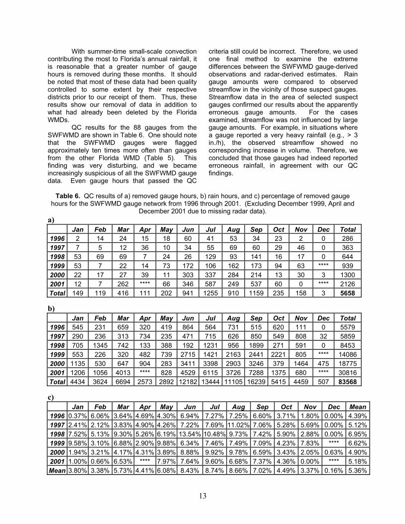
QC results for the 88 gauges from theSWFWMD are shown in Table 6. One should notethat the SWFWMD gauges were flaggedapproximately ten times more often than gaugesfrom the other Florida WMD (Table 5). Thisfinding was very disturbing, and we becameincreasingly suspicious of all the SWFWMD gaugedata. Even gauge hours that passed the QC

criteria still could be incorrect. Therefore, we usedone final method to examine the extremedifferences between the SWFWMD gauge-derivedobservations and radar-derived estimates. Raingauge amounts were compared to observedstreamflow in the vicinity of those suspect gauges.Streamflow data in the area of selected suspectgauges confirmed our results about the apparentlyerroneous gauge amounts. For the casesexamined, streamflow was not influenced by largegauge amounts. For example, in situations wherea gauge reported a very heavy rainfall (e.g., > 3in./h), the observed streamflow showed nocorresponding increase in volume. Therefore, weconcluded that those gauges had indeed reportederroneous rainfall, in agreement with our QCfindings.

Table 6. QC results of a) removed gauge hours, b) rain hours, and c) percentage of removed gaugehours for the SWFWMD gauge network from 1996 through 2001. (Excluding December 1999, April and

December 2001 due to missing radar data).a)

Jan Feb Mar Apr May Jun Jul Aug Sep Oct Nov Dec Total1996 2 14 24 15 18 60 41 53 34 23 2 0 2861997 7 5 12 36 10 34 55 69 60 29 46 0 3631998 53 69 69 7 24 26 129 93 141 16 17 0 6441999 53 7 22 14 73 172 106 162 173 94 63 **** 9392000 22 17 27 39 11 303 337 284 214 13 30 3 13002001 12 7 262 **** 66 346 587 249 537 60 0 **** 2126Total 149 119 416 111 202 941 1255 910 1159 235 158 3 5658

b)Jan Feb Mar Apr May Jun Jul Aug Sep Oct Nov Dec Total

1996 545 231 659 320 419 864 564 731 515 620 111 0 55791997 290 236 313 734 235 471 715 626 850 549 808 32 58591998 705 1345 742 133 388 192 1231 956 1899 271 591 0 84531999 553 226 320 482 739 2715 1421 2163 2441 2221 805 **** 140862000 1135 530 647 904 283 3411 3398 2903 3246 379 1464 475 187752001 1206 1056 4013 **** 828 4529 6115 3726 7288 1375 680 **** 30816Total 4434 3624 6694 2573 2892 12182 13444 11105 16239 5415 4459 507 83568

c)Jan Feb Mar Apr May Jun Jul Aug Sep Oct Nov Dec Mean

1996 0.37% 6.06% 3.64% 4.69% 4.30% 6.94% 7.27% 7.25% 6.60% 3.71% 1.80% 0.00% 4.39%1997 2.41% 2.12% 3.83% 4.90% 4.26% 7.22% 7.69% 11.02% 7.06% 5.28% 5.69% 0.00% 5.12%1998 7.52% 5.13% 9.30% 5.26% 6.19% 13.54% 10.48% 9.73% 7.42% 5.90% 2.88% 0.00% 6.95%1999 9.58% 3.10% 6.88% 2.90% 9.88% 6.34% 7.46% 7.49% 7.09% 4.23% 7.83% **** 6.62%2000 1.94% 3.21% 4.17% 4.31% 3.89% 8.88% 9.92% 9.78% 6.59% 3.43% 2.05% 0.63% 4.90%2001 1.00% 0.66% 6.53% **** 7.97% 7.64% 9.60% 6.68% 7.37% 4.36% 0.00% **** 5.18%Mean 3.80% 3.38% 5.73% 4.41% 6.08% 8.43% 8.74% 8.66% 7.02% 4.49% 3.37% 0.16% 5.36%

14

Based on these various investigations, wewere tempted to delete all of the SWFWMD gaugedata. However, that was not feasible because theMPE procedure requires some gauge data tocalculate the radar biases. Our guiding principlewas to use fewer quality gauges instead of alarger number of suspect gauges. Therefore, wedevised a procedure to identify the best of theSWFWMD gauges. We ranked the 88 SWFWMDgauges by the number of times each was flaggedby the QC procedure, and then performed amanual inspection of the gauge data. Theobjective was to establish a cutoff value forgauges to be kept versus those to be deleted.The gauges that were flagged the least wereassumed to be most accurate. Unfortunately,results of the ranking did not reveal a cleardistinction between “good vs. bad” gauges.Instead, the various gauges exhibited a relativelyuniform increase in the number of hours that wereflagged.

After an extensive analysis of the data, wedecided to keep the best 30% of the reporting(operational) gauges for each particular year. The30% threshold was chosen since it allowed theminimum number of gauges needed for MPEcalculations. For example, during 1999, 73gauges reported hourly rainfall amounts. Of these73 gauges, the best 30% to be kept yielded 22gauges as input to MPE. This procedurerepresents our attempt to make best use of whatappears to be an error-laden dataset from theSWFWMD.

The OH dataset contained many gauges(~ 85%) that reported and truncated rainfallamounts to the nearest 0.10 in. (not 0.01 in.). Inaddressing this issue, we increased non-zerogauge amounts by 0.05 in. to minimize some ofthe error associated with the truncation. This is animperfect solution to the problem. Since amountsless than 0.10 in. had been reported as 0.00 in.,there was no feasible way to distinguish betweenhours with truly zero amounts from those less than0.10 in. but reported as zero. After applying the0.05 in. increase to all gauges reporting at least0.1 in., the data were input to the QC proceduredescribed previously. Results (not shown)indicated that the percentages of removed hoursare approximately 4-5 times greater than for theFlorida WMD network (Table 4c), with the greatestamounts also occurring during summer. Thus, theOH data appear to be less reliable than those from

the Florida WMDs (with the exception ofSWFWMD data).

4. RESULTS

4.1 Seasonal Product ComparisonsTo compare and evaluate the various

MPE-derived precipitation estimates, hourly gridpoint values were summed for each season of thestudy period (1996 through 2001). Warm seasonmonths consisted of April through September,while cold season months included Octoberthrough March. Spatial depictions of four MPEproducts (RMOSAIC, GMOSAIC, BMOSAIC, andMMOSAIC) then were generated. Results for twowarm seasons and one cold season are presentedhere.

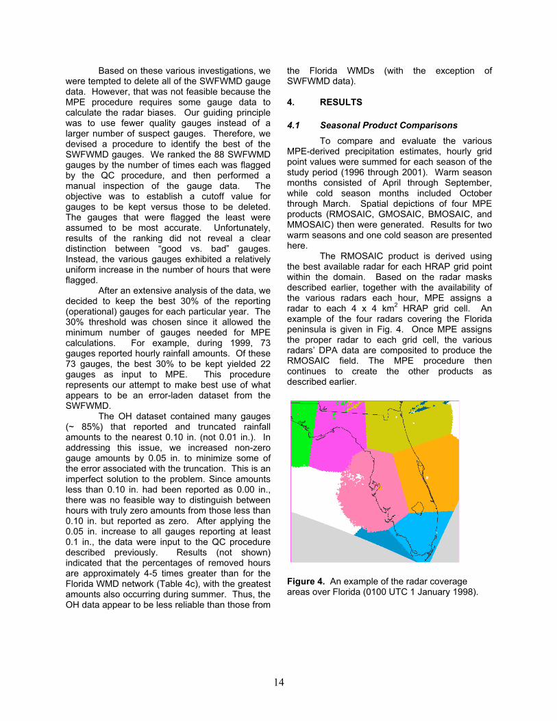
The RMOSAIC product is derived usingthe best available radar for each HRAP grid pointwithin the domain. Based on the radar masksdescribed earlier, together with the availability ofthe various radars each hour, MPE assigns aradar to each 4 x 4 km2 HRAP grid cell. Anexample of the four radars covering the Floridapeninsula is given in Fig. 4. Once MPE assignsthe proper radar to each grid cell, the variousradars’ DPA data are composited to produce theRMOSAIC field. The MPE procedure thencontinues to create the other products asdescribed earlier.

Figure 4. An example of the radar coverageareas over Florida (0100 UTC 1 January 1998).

15

a) b)

c) d)

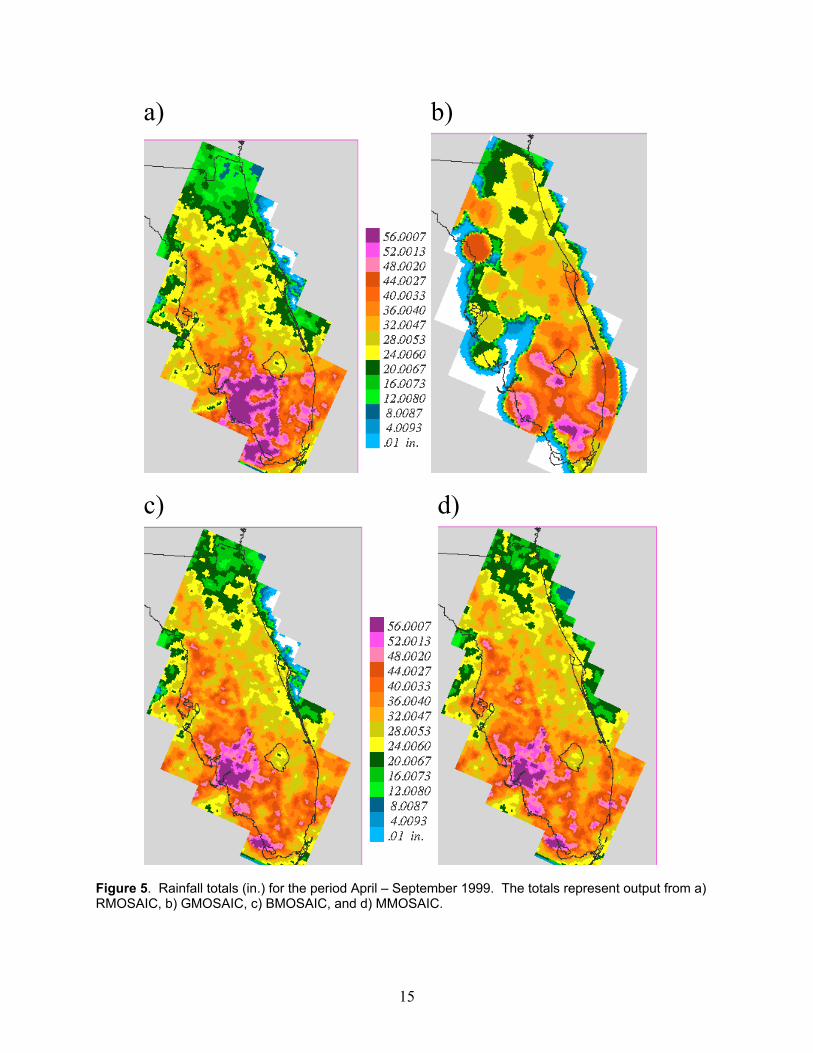
Figure 5. Rainfall totals (in.) for the period April – September 1999. The totals represent output from a)RMOSAIC, b) GMOSAIC, c) BMOSAIC, and d) MMOSAIC.

16

a) b)

c) d)

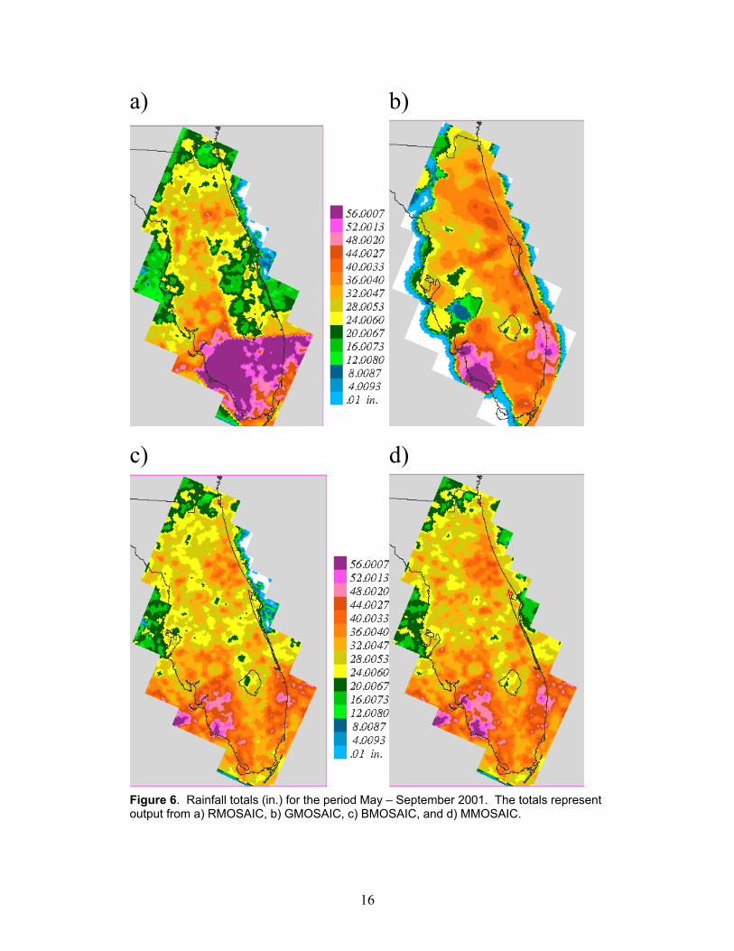
Figure 6. Rainfall totals (in.) for the period May – September 2001. The totals representoutput from a) RMOSAIC, b) GMOSAIC, c) BMOSAIC, and d) MMOSAIC.

17

a) b)

c) d)

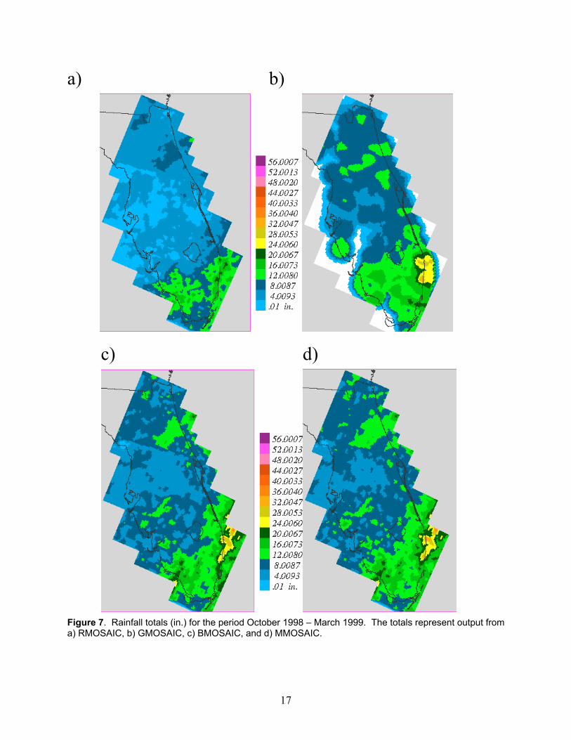
Figure 7. Rainfall totals (in.) for the period October 1998 – March 1999. The totals represent output froma) RMOSAIC, b) GMOSAIC, c) BMOSAIC, and d) MMOSAIC.

18

RMOSAIC fields for our period of studyare shown in panels a) of Figs. 5-7. One shouldnote the distinct lines of demarcation that areevident over the peninsula during some warmseasons (e.g., Figs. 5a and 6a). These linescorrespond to boundaries in the radar indexproduct (Fig. 4). For example, during the warmseason of 2001 (Fig. 6a), the Melbourne (MLB)radar (Fig. 2) appears “cold” (underestimation ofradar-derived rainfall) compared with thesurrounding radars, while estimates from theMiami radar (AMX) appear too large (“hot”).

Two factors appear to explain thesedistinct gradients between radars. One possibilityinvolves the Z-R relationship used at each radarsite. Utilizing a tropical Z-R relationship duringnon-tropical conditions will yield an overestimate inrainfall. Personnel at NWS-Miami confirmed thatthe AMX radar predominantly operated in thetropical Z-R mode during the warm season of2001 (Fig. 6a). In addition, poor calibration at aradar site can contribute to the “lines” in theprecipitation pattern. Since each radar has its owncalibration, improper calibrations will yield adiscontinuity at the boundaries. Although distinctlines of demarcation between radar boundariesare most clearly evident during some warmseasons, the winter season months also canexhibit this feature, but to a lesser degree. Notevery old or warm season exhibits discontinuitiesbetween radars. In Fig. 7a for example, there areno distinct gradients that can be attributed to theparticular radar being used. RMOSAIC showsreasonable rainfall patterns with the appropriatespatial detail.

In summary, the RMOSAIC maps providean excellent spatial depiction of Florida rainfall;however, actual values sometimes appear suspectdue to improper calibrations or Z-R relations.

The GMOSAIC product of MPE utilizesonly gauges in its calculations. Since gaugesgenerally are considered to be “ground truth”, theyare used in many meteorological and hydrologicaloperations. However, an analysis of theGMOSAIC maps during the study period illustratessome of the shortcomings of using gauges alone.As noted earlier, a gauge value is assigned acertain radius of influence (ROI). Figure 5b showsindividual gauge amounts being assigned tocircular ROI regions in the northwestern portion ofthe domain where there are relatively few gauges.Conversely, the GMOSAIC field is much smootherin areas with a dense gauge network, e.g., theeastern and southern parts of the domain.

Another noticeable characteristic of theGMOSAIC field is the effective coverage area of

the gauges. Although the SWFWMD maintains adense gauge network, we were forced to deletemuch of their data because of the quality controlissues described earlier. This effect is clearlynoticeable as the bare area between Tampa andLake Okeechobee (e.g., Fig. 5b). Although thislack of gauges affects the bias calculations inMPE, it is nonetheless better to use fewer, higherquality gauges, than more, less-quality gauges.

The warm season GMOSAIC fields showmany cases where large differences exist betweenadjacent gauges (Fig. 5-6b). Although one couldargue that suspect data had passed through ourQC procedure, such patterns can be seenthroughout the GMOSAIC images, suggesting thatthey are due to the highly variable convectiverainfall.

The cold season GMOSAIC analysesexhibit a more uniform rainfall pattern than duringthe warm season. Despite some relatively heavyamounts in southeastern Florida (e.g., Fig. 7b),cold season rainfall typically is fairly uniformacross the peninsula, with amounts generallyranging between 8 – 12 in. One should note thatthe GMOSAIC amounts tend to be greater thanthose from the radar during the cool seasons (Fig,7a vs. Fig. 7b), probably due to the radar beamfrequently overshooting the relatively low tops ofstratiform clouds. A goal of the MPE procedure isto reduce these radar underestimates.

The BMOSAIC product of MPE blends theGMOSAIC and RMOSAIC products to maximizethe strengths of both gauges and radars.BMOSAIC is based on a radar-wide bias for eachradar that is applied to the original radar-derived(RMOSAIC) estimates, thereby removing the area-wide biases for each radar. One noticeablecharacteristic of BMOSAIC is its ability to greatlyreduce the “hot/cold” issues contained in theoriginal RMOSAIC fields (Figs. 5c and 6c).However, in Fig. 5c, a slight discontinuity stillexists even after the bias adjustment. This line ofdemarcation will be described further insubsequent sections. During the cold season (Fig.7c), values of BMOSAIC are greater than thosefrom the RMOSAIC, showing the adjustmentprovided by the gauges.

The final product of MPE (MMOSAIC)incorporates gauge values (GMOSAIC) with thebias-corrected radar values (BMOSAIC) tocalculate local adjustments. The c) and d) panelsof Figs. 5-7 show that differences betweenBMOSAIC and MMOSAIC are subtle. Severaladaptable parameters within MPE define therelative strengths of the input gauges and theradars, while simultaneously minimizing the

19

adverse affects of each source alone. Werigorously tested many combinations of three keyadaptable parameters within MPE--the “gaugeradius of influence” (ROI), the lag-0 indicatorcross-correlation, and the lag-0 conditional crosscorrelation. Consulting with personnel at NWS OH,they proposed modifications to the adaptableparameters to maximize the desirable effects ofMPE (Seo 2004, personal communication). Afterimplementing these changes, the final set ofadaptable parameters was chosen (describedearlier).

The summer 1999 period was the focus ofmany test runs (Fig. 5). Our goals were to achievethe most representative MPE products, andpossibly to remove the line of discontinuity throughcentral Florida. This straight “line” is evident in theRMOSAIC, BMOSAIC, and MMOSAIC maps(Figs. 5a, c, d). Since much of the SWFWMDgauge data had been deleted, the “line” is duepartly to sparse gauge data being input to MPE tocalculate radar-wide biases. However, the “line”also exists in the radar data (RMOSAIC, Fig. 5a),probably due to calibration issues. Thedemarcation was not expected in the BMOSAICand MMOSAIC fields (Figs. 5c, d) since the MPEscheme is designed to correct the radar data withcorresponding gauge data. The “line” appears tocoincide with the index masks between the Tampa(TBW) and MLB radars (Fig. 4). Discussions withNWS OH personnel revealed that similardemarcation problems have been discovered inother areas of the country. They are mostnoticeable at longer time scales (e.g., monthly,seasonally, or yearly) (Bradberry, 2004, personalcommunication).

We believe that there also is some realenhancement of precipitation over central Floridaduring summer 1999. This is suggested by theenhanced GMOSAIC values in central Florida(Fig. 5b). On relatively light wind days, the Atlanticand Gulf Coast sea breezes often converge overthe central portion of the state producing amaximum of precipitation down the spine ofFlorida. Thus, we believe that the north-south“line” in Fig. 5d is partly “real”, and partly due toMPE’s inability to remove all of the area-wideradar biases. This one season illustrates all of theinherent problems with gauges, radars, the MPEscheme, and even the natural variability of Floridarainfall.

MPE does an exemplary job of removingradar index lines during the warm season of 2001(Fig. 6). RMOSAIC exhibits a sharp discontinuitybetween radars (Fig. 6a); however, both theBMOSAIC and MMOSAIC fields (Figs. 6c and 6d,

respectively) exhibit a reasonable depiction ofpeninsula precipitation. Thus, the gaugecorrections applied by MPE achieve their goal.

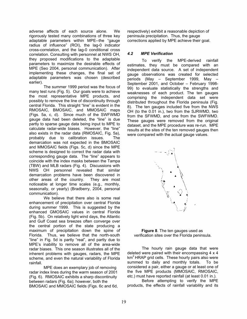
4.2 MPE VerificationTo verify the MPE-derived rainfall

estimates, they must be compared with anindependent data source. A set of independentgauge observations was created for selectedperiods (May – September 1999, May –September 2001, and October – February 1998-99) to evaluate statistically the strengths andweaknesses of each product. The ten gaugescomprising the independent data set weredistributed throughout the Florida peninsula (Fig.8). The ten gauges included five from the NWSOH (to the 0.01 in.), two from the SJRWMD, twofrom the SFWMD, and one from the SWFWMD.These gauges were removed from the originaldataset, and the MPE procedure was re-run. MPEresults at the sites of the ten removed gauges thenwere compared with the actual gauge values.

Figure 8. The ten gauges used as verification sites over the Florida peninsula.

The hourly rain gauge data that weredeleted were paired with their encompassing 4 x 4km2 HRAP grid cells. These hourly pairs also weresummed to daily and monthly totals. To beconsidered a pair, either a gauge or at least one ofthe five MPE products (MMOSAIC, RMOSAIC,etc.) must have reported rainfall (at least 0.01 in.).

Before attempting to verify the MPEproducts, the effects of rainfall variability and its

20

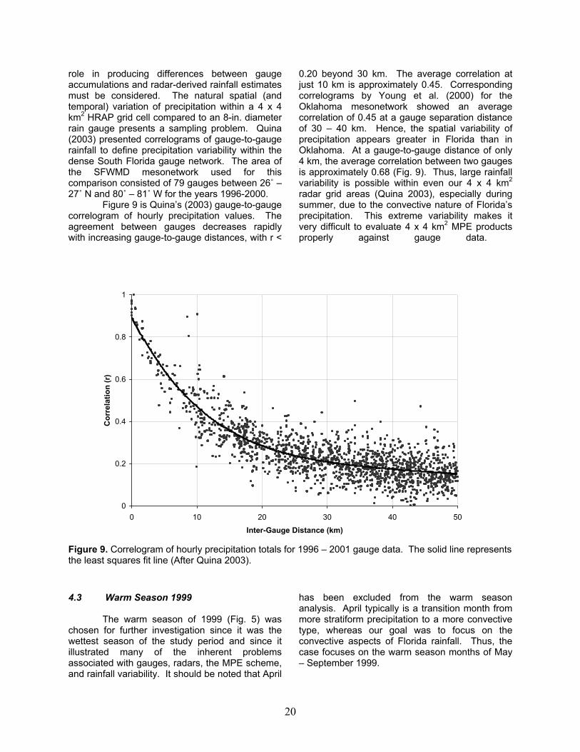
role in producing differences between gaugeaccumulations and radar-derived rainfall estimatesmust be considered. The natural spatial (andtemporal) variation of precipitation within a 4 x 4km2 HRAP grid cell compared to an 8-in. diameterrain gauge presents a sampling problem. Quina(2003) presented correlograms of gauge-to-gaugerainfall to define precipitation variability within thedense South Florida gauge network. The area ofthe SFWMD mesonetwork used for thiscomparison consisted of 79 gauges between 26˚ –27˚ N and 80˚ – 81˚ W for the years 1996-2000.

Figure 9 is Quina’s (2003) gauge-to-gaugecorrelogram of hourly precipitation values. Theagreement between gauges decreases rapidlywith increasing gauge-to-gauge distances, with r <

0.20 beyond 30 km. The average correlation atjust 10 km is approximately 0.45. Correspondingcorrelograms by Young et al. (2000) for theOklahoma mesonetwork showed an averagecorrelation of 0.45 at a gauge separation distanceof 30 – 40 km. Hence, the spatial variability ofprecipitation appears greater in Florida than inOklahoma. At a gauge-to-gauge distance of only4 km, the average correlation between two gaugesis approximately 0.68 (Fig. 9). Thus, large rainfallvariability is possible within even our 4 x 4 km2

radar grid areas (Quina 2003), especially duringsummer, due to the convective nature of Florida’sprecipitation. This extreme variability makes itvery difficult to evaluate 4 x 4 km2 MPE productsproperly against gauge data.

Figure 9. Correlogram of hourly precipitation totals for 1996 – 2001 gauge data. The solid line representsthe least squares fit line (After Quina 2003).

4.3 Warm Season 1999

The warm season of 1999 (Fig. 5) waschosen for further investigation since it was thewettest season of the study period and since itillustrated many of the inherent problemsassociated with gauges, radars, the MPE scheme,and rainfall variability. It should be noted that April

has been excluded from the warm seasonanalysis. April typically is a transition month frommore stratiform precipitation to a more convectivetype, whereas our goal was to focus on theconvective aspects of Florida rainfall. Thus, thecase focuses on the warm season months of May– September 1999.

0

0.2

0.4

0.6

0.8

1

0 10 20 30 40 50

Inter-Gauge Distance (km)

Cor

rela

tion

(r)

21

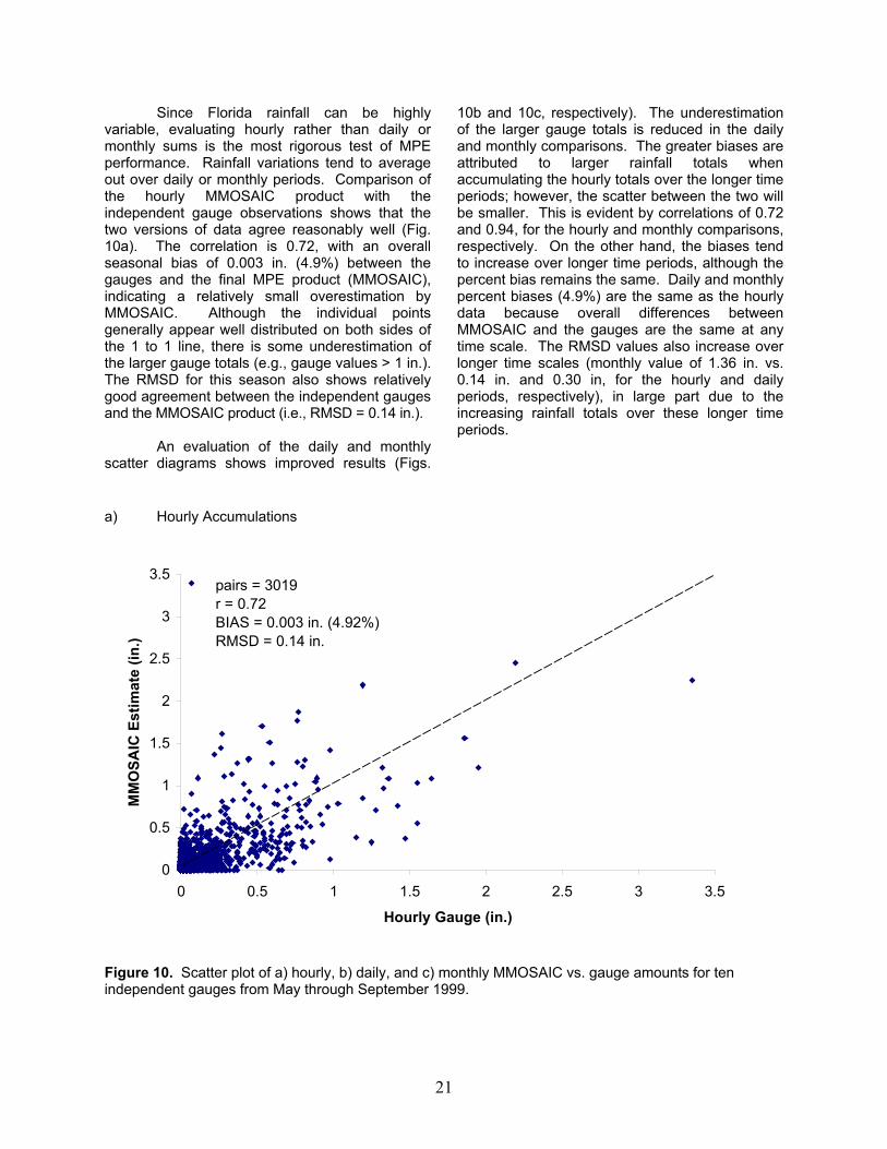
Since Florida rainfall can be highlyvariable, evaluating hourly rather than daily ormonthly sums is the most rigorous test of MPEperformance. Rainfall variations tend to averageout over daily or monthly periods. Comparison ofthe hourly MMOSAIC product with theindependent gauge observations shows that thetwo versions of data agree reasonably well (Fig.10a). The correlation is 0.72, with an overallseasonal bias of 0.003 in. (4.9%) between thegauges and the final MPE product (MMOSAIC),indicating a relatively small overestimation byMMOSAIC. Although the individual pointsgenerally appear well distributed on both sides ofthe 1 to 1 line, there is some underestimation ofthe larger gauge totals (e.g., gauge values > 1 in.).The RMSD for this season also shows relativelygood agreement between the independent gaugesand the MMOSAIC product (i.e., RMSD = 0.14 in.).

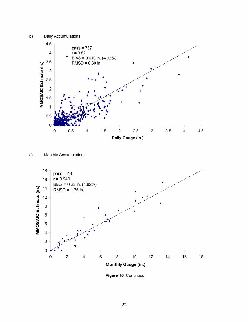
An evaluation of the daily and monthlyscatter diagrams shows improved results (Figs.

10b and 10c, respectively). The underestimationof the larger gauge totals is reduced in the dailyand monthly comparisons. The greater biases areattributed to larger rainfall totals whenaccumulating the hourly totals over the longer timeperiods; however, the scatter between the two willbe smaller. This is evident by correlations of 0.72and 0.94, for the hourly and monthly comparisons,respectively. On the other hand, the biases tendto increase over longer time periods, although thepercent bias remains the same. Daily and monthlypercent biases (4.9%) are the same as the hourlydata because overall differences betweenMMOSAIC and the gauges are the same at anytime scale. The RMSD values also increase overlonger time scales (monthly value of 1.36 in. vs.0.14 in. and 0.30 in, for the hourly and dailyperiods, respectively), in large part due to theincreasing rainfall totals over these longer timeperiods.

a) Hourly Accumulations

0

0.5

1

1.5

2

2.5

3

3.5

0 0.5 1 1.5 2 2.5 3 3.5

Hourly Gauge (in.)

MM

OSA

IC E

stim

ate

(in.)

pairs = 3019r = 0.72BIAS = 0.003 in. (4.92%)RMSD = 0.14 in.

Figure 10. Scatter plot of a) hourly, b) daily, and c) monthly MMOSAIC vs. gauge amounts for tenindependent gauges from May through September 1999.

22

b) Daily Accumulations

0

0.5

1

1.5

2

2.5

3

3.5

4

4.5

0 0.5 1 1.5 2 2.5 3 3.5 4 4.5

Daily Gauge (in.)

MM

OSA

IC E

stim

ate

(in.)


c) Monthly Accumulations

0

2

4

6

8

10

12

14

16

18

0 2 4 6 8 10 12 14 16 18

Monthly Gauge (in.)

MM

OSA

IC E

stim

ate

(in.)


Figure 10. Continued.

23

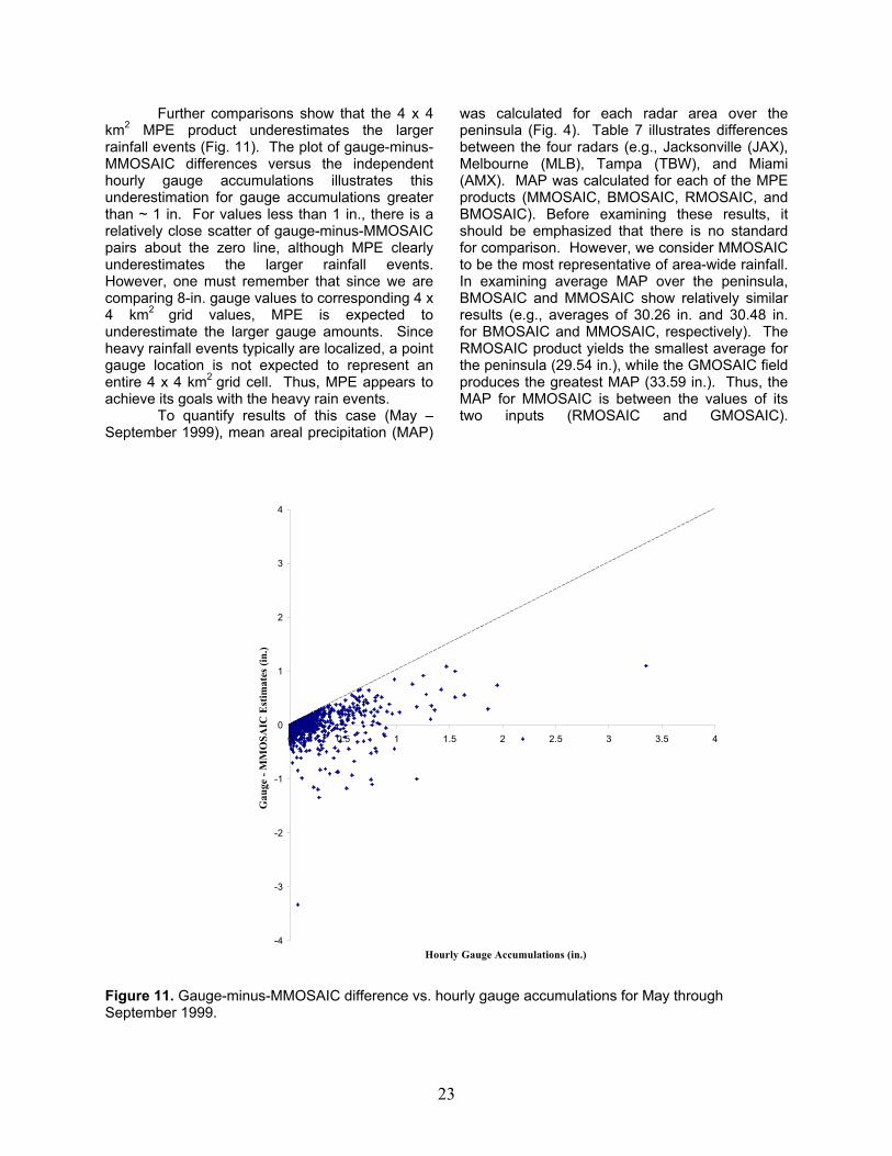
Further comparisons show that the 4 x 4km2 MPE product underestimates the largerrainfall events (Fig. 11). The plot of gauge-minus-MMOSAIC differences versus the independenthourly gauge accumulations illustrates thisunderestimation for gauge accumulations greaterthan ~ 1 in. For values less than 1 in., there is arelatively close scatter of gauge-minus-MMOSAICpairs about the zero line, although MPE clearlyunderestimates the larger rainfall events.However, one must remember that since we arecomparing 8-in. gauge values to corresponding 4 x4 km2 grid values, MPE is expected tounderestimate the larger gauge amounts. Sinceheavy rainfall events typically are localized, a pointgauge location is not expected to represent anentire 4 x 4 km2 grid cell. Thus, MPE appears toachieve its goals with the heavy rain events.

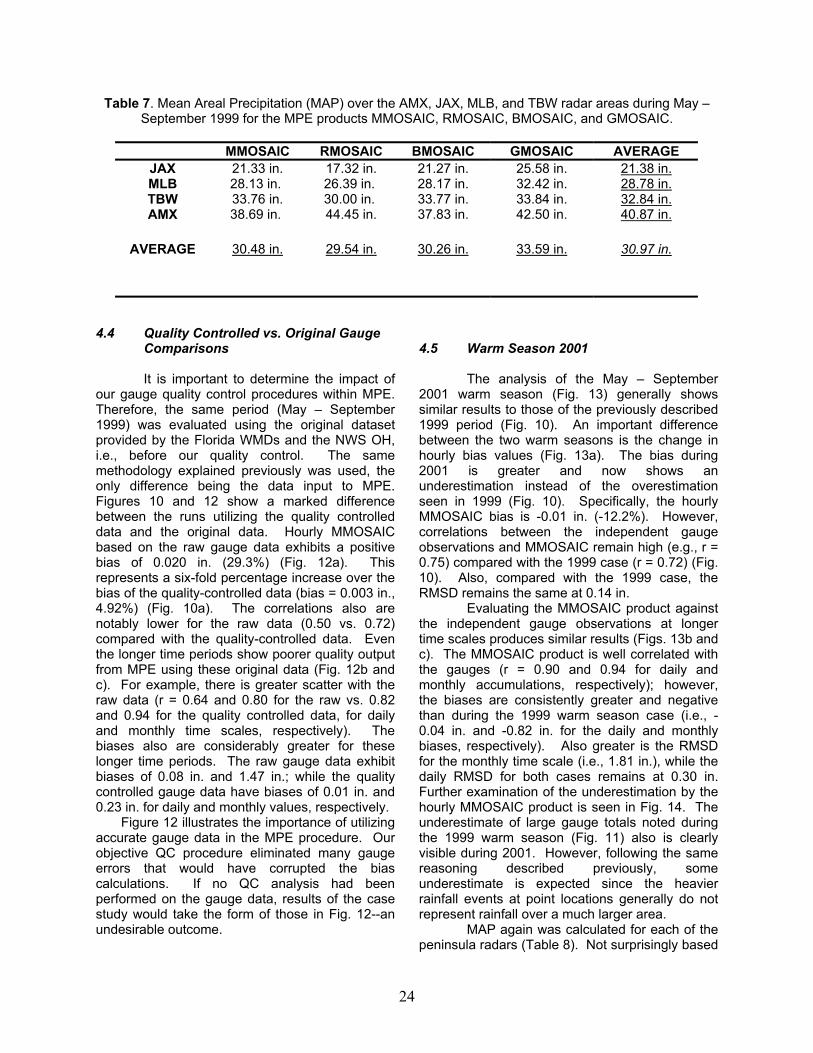
To quantify results of this case (May –September 1999), mean areal precipitation (MAP)

was calculated for each radar area over thepeninsula (Fig. 4). Table 7 illustrates differencesbetween the four radars (e.g., Jacksonville (JAX),Melbourne (MLB), Tampa (TBW), and Miami(AMX). MAP was calculated for each of the MPEproducts (MMOSAIC, BMOSAIC, RMOSAIC, andBMOSAIC). Before examining these results, itshould be emphasized that there is no standardfor comparison. However, we consider MMOSAICto be the most representative of area-wide rainfall.In examining average MAP over the peninsula,BMOSAIC and MMOSAIC show relatively similarresults (e.g., averages of 30.26 in. and 30.48 in.for BMOSAIC and MMOSAIC, respectively). TheRMOSAIC product yields the smallest average forthe peninsula (29.54 in.), while the GMOSAIC fieldproduces the greatest MAP (33.59 in.). Thus, theMAP for MMOSAIC is between the values of itstwo inputs (RMOSAIC and GMOSAIC).

Figure 11. Gauge-minus-MMOSAIC difference vs. hourly gauge accumulations for May throughSeptember 1999.

-4

-3

-2

-1

0

1

2

3

4

0 0.5 1 1.5 2 2.5 3 3.5 4

Hourly Gauge Accumulations (in.)

Gau

ge -

MM

OSA

IC E

stim

ates

(in.

)

24

Table 7. Mean Areal Precipitation (MAP) over the AMX, JAX, MLB, and TBW radar areas during May –September 1999 for the MPE products MMOSAIC, RMOSAIC, BMOSAIC, and GMOSAIC.

MMOSAIC RMOSAIC BMOSAIC GMOSAIC AVERAGEJAX 21.33 in. 17.32 in. 21.27 in. 25.58 in. 21.38 in.MLB 28.13 in. 26.39 in. 28.17 in. 32.42 in. 28.78 in.TBW 33.76 in. 30.00 in. 33.77 in. 33.84 in. 32.84 in.AMX 38.69 in. 44.45 in. 37.83 in. 42.50 in. 40.87 in.

AVERAGE 30.48 in. 29.54 in. 30.26 in. 33.59 in. 30.97 in.

4.4 Quality Controlled vs. Original GaugeComparisons

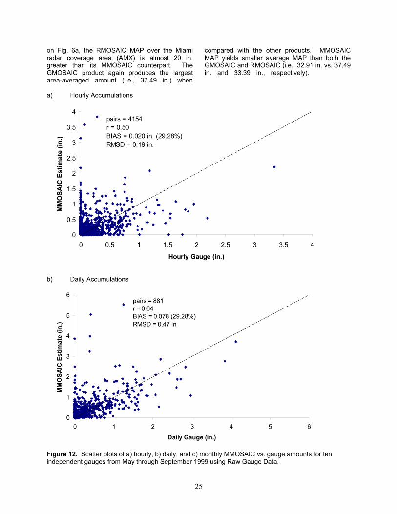
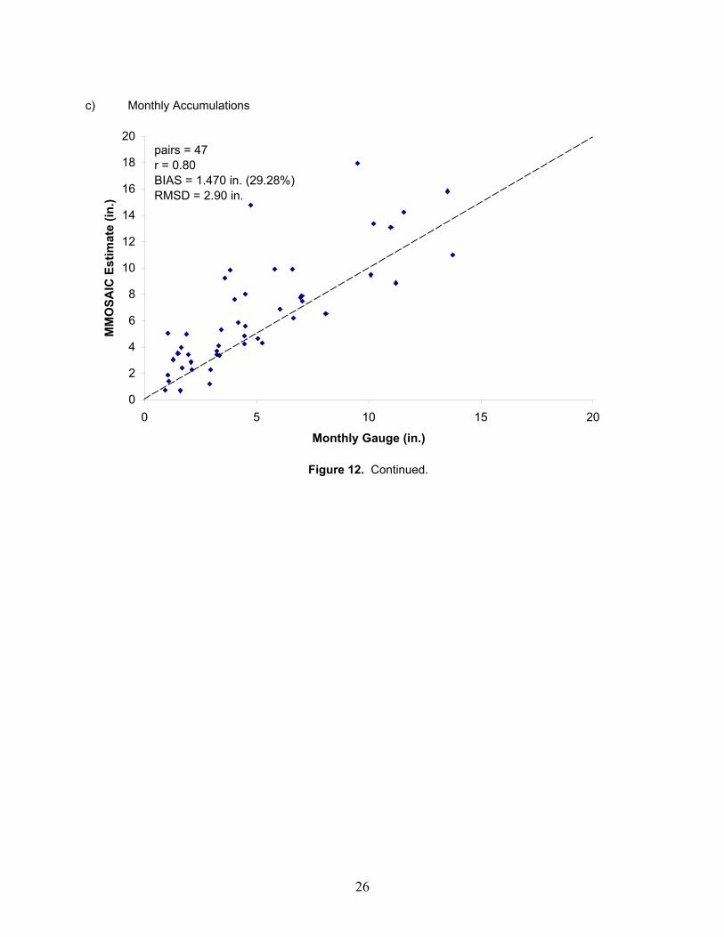
It is important to determine the impact ofour gauge quality control procedures within MPE.Therefore, the same period (May – September1999) was evaluated using the original datasetprovided by the Florida WMDs and the NWS OH,i.e., before our quality control. The samemethodology explained previously was used, theonly difference being the data input to MPE.Figures 10 and 12 show a marked differencebetween the runs utilizing the quality controlleddata and the original data. Hourly MMOSAICbased on the raw gauge data exhibits a positivebias of 0.020 in. (29.3%) (Fig. 12a). Thisrepresents a six-fold percentage increase over thebias of the quality-controlled data (bias = 0.003 in.,4.92%) (Fig. 10a). The correlations also arenotably lower for the raw data (0.50 vs. 0.72)compared with the quality-controlled data. Eventhe longer time periods show poorer quality outputfrom MPE using these original data (Fig. 12b andc). For example, there is greater scatter with theraw data (r = 0.64 and 0.80 for the raw vs. 0.82and 0.94 for the quality controlled data, for dailyand monthly time scales, respectively). Thebiases also are considerably greater for theselonger time periods. The raw gauge data exhibitbiases of 0.08 in. and 1.47 in.; while the qualitycontrolled gauge data have biases of 0.01 in. and0.23 in. for daily and monthly values, respectively. Figure 12 illustrates the importance of utilizingaccurate gauge data in the MPE procedure. Ourobjective QC procedure eliminated many gaugeerrors that would have corrupted the biascalculations. If no QC analysis had beenperformed on the gauge data, results of the casestudy would take the form of those in Fig. 12--anundesirable outcome.

4.5 Warm Season 2001

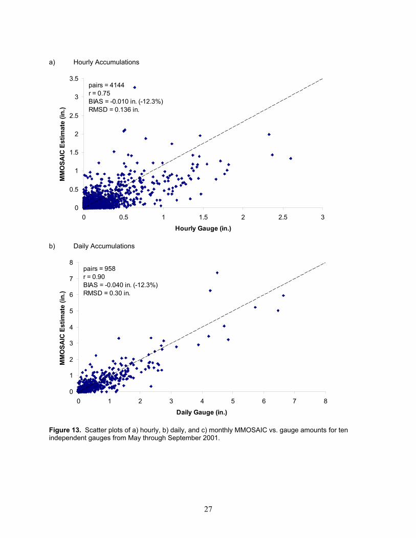
The analysis of the May – September2001 warm season (Fig. 13) generally showssimilar results to those of the previously described1999 period (Fig. 10). An important differencebetween the two warm seasons is the change inhourly bias values (Fig. 13a). The bias during2001 is greater and now shows anunderestimation instead of the overestimationseen in 1999 (Fig. 10). Specifically, the hourlyMMOSAIC bias is -0.01 in. (-12.2%). However,correlations between the independent gaugeobservations and MMOSAIC remain high (e.g., r =0.75) compared with the 1999 case (r = 0.72) (Fig.10). Also, compared with the 1999 case, theRMSD remains the same at 0.14 in.

Evaluating the MMOSAIC product againstthe independent gauge observations at longertime scales produces similar results (Figs. 13b andc). The MMOSAIC product is well correlated withthe gauges (r = 0.90 and 0.94 for daily andmonthly accumulations, respectively); however,the biases are consistently greater and negativethan during the 1999 warm season case (i.e., -0.04 in. and -0.82 in. for the daily and monthlybiases, respectively). Also greater is the RMSDfor the monthly time scale (i.e., 1.81 in.), while thedaily RMSD for both cases remains at 0.30 in.Further examination of the underestimation by thehourly MMOSAIC product is seen in Fig. 14. Theunderestimate of large gauge totals noted duringthe 1999 warm season (Fig. 11) also is clearlyvisible during 2001. However, following the samereasoning described previously, someunderestimate is expected since the heavierrainfall events at point locations generally do notrepresent rainfall over a much larger area.

MAP again was calculated for each of thepeninsula radars (Table 8). Not surprisingly based

25

on Fig. 6a, the RMOSAIC MAP over the Miamiradar coverage area (AMX) is almost 20 in.greater than its MMOSAIC counterpart. TheGMOSAIC product again produces the largestarea-averaged amount (i.e., 37.49 in.) when

compared with the other products. MMOSAICMAP yields smaller average MAP than both theGMOSAIC and RMOSAIC (i.e., 32.91 in. vs. 37.49in. and 33.39 in., respectively).


0

0.5

1

1.5

2

2.5

3

3.5

4

0 0.5 1 1.5 2 2.5 3 3.5 4

Hourly Gauge (in.)

MM

OSA

IC E

stim

ate

(in.)



0

1

2

3

4

5

6

0 1 2 3 4 5 6

Daily Gauge (in.)

MM

OSA

IC E

stim

ate

(in.)

pairs = 881r = 0.64BIAS = 0.078 (29.28%)RMSD = 0.47 in.

Figure 12. Scatter plots of a) hourly, b) daily, and c) monthly MMOSAIC vs. gauge amounts for tenindependent gauges from May through September 1999 using Raw Gauge Data.

26


0

2

4

6

8

10

12

14

16

18

20

0 5 10 15 20

Monthly Gauge (in.)

MM

OSA

IC E

stim

ate

(in.)



27


0

0.5

1

1.5

2

2.5

3

3.5

0 0.5 1 1.5 2 2.5 3

Hourly Gauge (in.)

MM

OSA

IC E

stim

ate

(in.)

pairs = 4144r = 0.75BIAS = -0.010 in. (-12.3%)RMSD = 0.136 in.


0

1

2

3

4

5

6

7

8

0 1 2 3 4 5 6 7 8

Daily Gauge (in.)

MM

OSA

IC E

stim

ate

(in.)


Figure 13. Scatter plots of a) hourly, b) daily, and c) monthly MMOSAIC vs. gauge amounts for tenindependent gauges from May through September 2001.

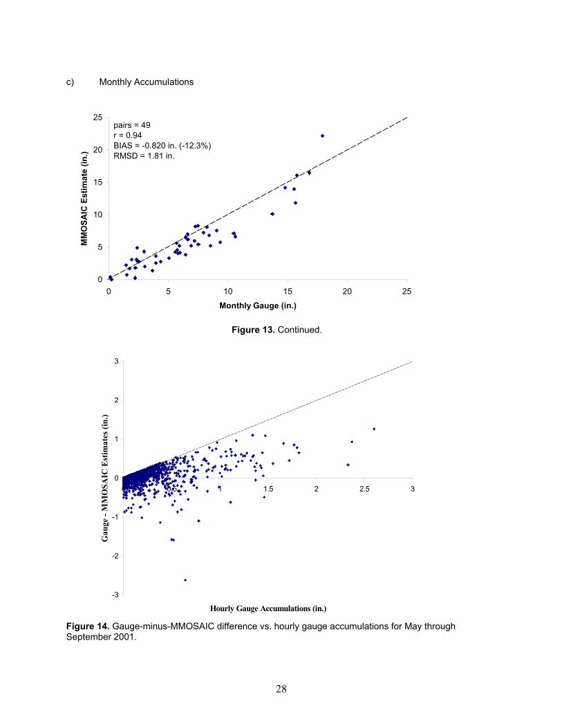
28


0

5

10

15

20

25

0 5 10 15 20 25

Monthly Gauge (in.)

MM

OSA

IC E

stim

ate

(in.)



Figure 14. Gauge-minus-MMOSAIC difference vs. hourly gauge accumulations for May throughSeptember 2001.

-3

-2

-1

0

1

2

3

0 0.5 1 1.5 2 2.5 3


Gau

ge -

MM

OSA

IC E

stim

ates

(in.

)

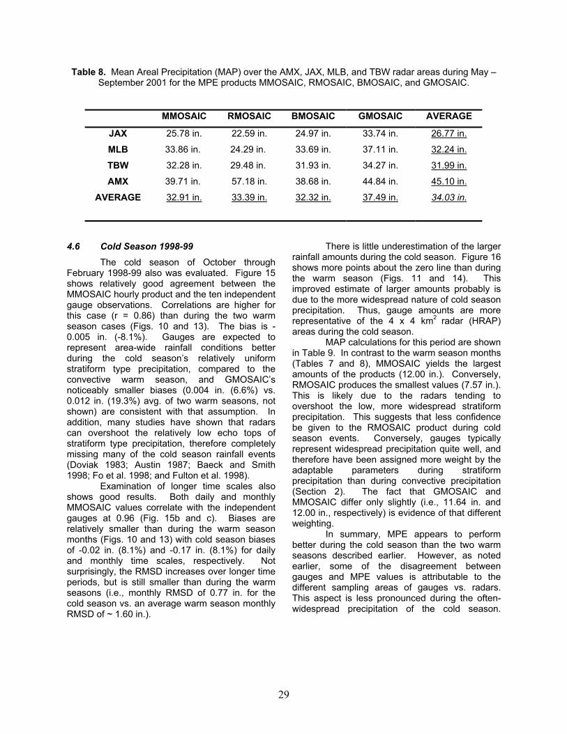
29

Table 8. Mean Areal Precipitation (MAP) over the AMX, JAX, MLB, and TBW radar areas during May –September 2001 for the MPE products MMOSAIC, RMOSAIC, BMOSAIC, and GMOSAIC.

MMOSAIC RMOSAIC BMOSAIC GMOSAIC AVERAGE

JAX 25.78 in. 22.59 in. 24.97 in. 33.74 in. 26.77 in.

MLB 33.86 in. 24.29 in. 33.69 in. 37.11 in. 32.24 in.

TBW 32.28 in. 29.48 in. 31.93 in. 34.27 in. 31.99 in.

AMX 39.71 in. 57.18 in. 38.68 in. 44.84 in. 45.10 in.


4.6 Cold Season 1998-99The cold season of October through

February 1998-99 also was evaluated. Figure 15shows relatively good agreement between theMMOSAIC hourly product and the ten independentgauge observations. Correlations are higher forthis case (r = 0.86) than during the two warmseason cases (Figs. 10 and 13). The bias is -0.005 in. (-8.1%). Gauges are expected torepresent area-wide rainfall conditions betterduring the cold season’s relatively uniformstratiform type precipitation, compared to theconvective warm season, and GMOSAIC’snoticeably smaller biases (0.004 in. (6.6%) vs.0.012 in. (19.3%) avg. of two warm seasons, notshown) are consistent with that assumption. Inaddition, many studies have shown that radarscan overshoot the relatively low echo tops ofstratiform type precipitation, therefore completelymissing many of the cold season rainfall events(Doviak 1983; Austin 1987; Baeck and Smith1998; Fo et al. 1998; and Fulton et al. 1998).

Examination of longer time scales alsoshows good results. Both daily and monthlyMMOSAIC values correlate with the independentgauges at 0.96 (Fig. 15b and c). Biases arerelatively smaller than during the warm seasonmonths (Figs. 10 and 13) with cold season biasesof -0.02 in. (8.1%) and -0.17 in. (8.1%) for dailyand monthly time scales, respectively. Notsurprisingly, the RMSD increases over longer timeperiods, but is still smaller than during the warmseasons (i.e., monthly RMSD of 0.77 in. for thecold season vs. an average warm season monthlyRMSD of ~ 1.60 in.).

There is little underestimation of the largerrainfall amounts during the cold season. Figure 16shows more points about the zero line than duringthe warm season (Figs. 11 and 14). Thisimproved estimate of larger amounts probably isdue to the more widespread nature of cold seasonprecipitation. Thus, gauge amounts are morerepresentative of the 4 x 4 km2 radar (HRAP)areas during the cold season.

MAP calculations for this period are shownin Table 9. In contrast to the warm season months(Tables 7 and 8), MMOSAIC yields the largestamounts of the products (12.00 in.). Conversely,RMOSAIC produces the smallest values (7.57 in.).This is likely due to the radars tending toovershoot the low, more widespread stratiformprecipitation. This suggests that less confidencebe given to the RMOSAIC product during coldseason events. Conversely, gauges typicallyrepresent widespread precipitation quite well, andtherefore have been assigned more weight by theadaptable parameters during stratiformprecipitation than during convective precipitation(Section 2). The fact that GMOSAIC andMMOSAIC differ only slightly (i.e., 11.64 in. and12.00 in., respectively) is evidence of that differentweighting.

In summary, MPE appears to performbetter during the cold season than the two warmseasons described earlier. However, as notedearlier, some of the disagreement betweengauges and MPE values is attributable to thedifferent sampling areas of gauges vs. radars.This aspect is less pronounced during the often-widespread precipitation of the cold season.

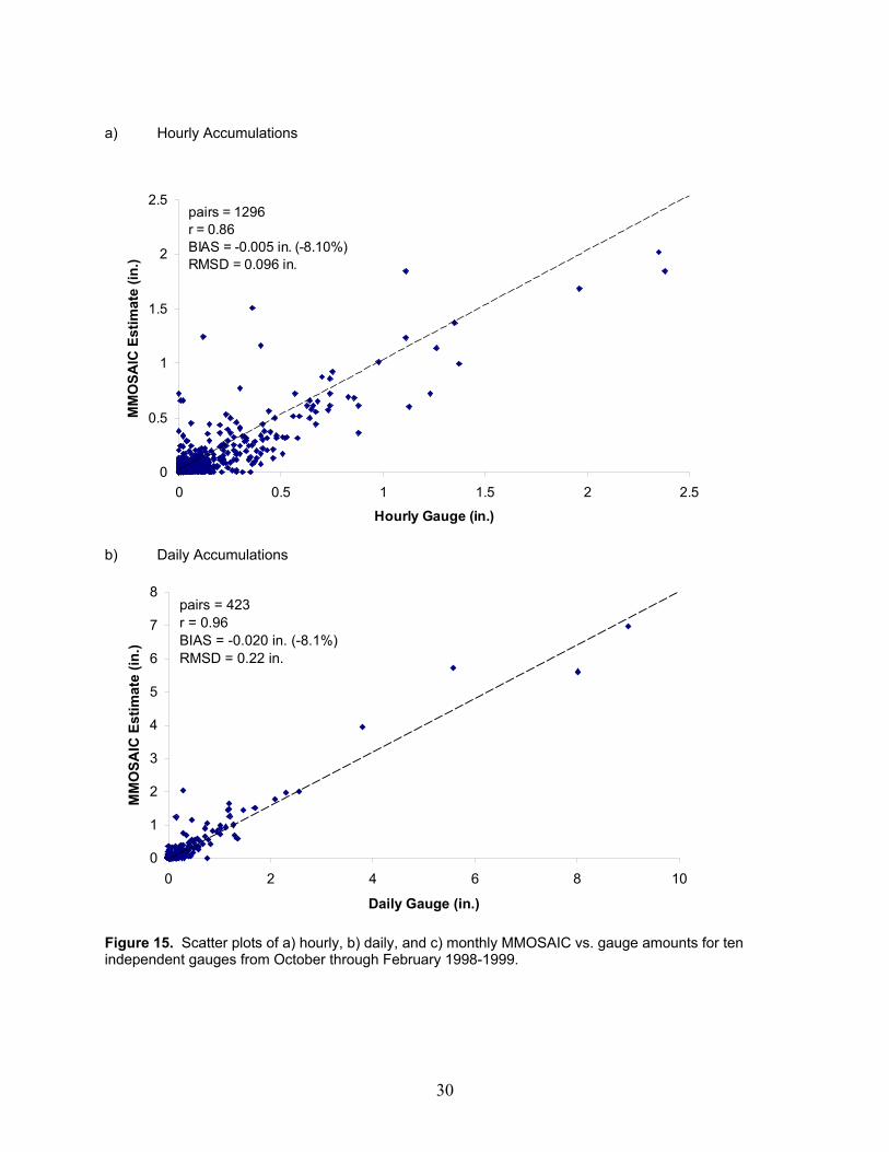
30


0

0.5

1

1.5

2

2.5

0 0.5 1 1.5 2 2.5

Hourly Gauge (in.)

MM

OSA

IC E

stim

ate

(in.)



0

1

2

3

4

5

6

7

8

0 2 4 6 8 10

Daily Gauge (in.)

MM

OSA

IC E

stim

ate

(in.)


Figure 15. Scatter plots of a) hourly, b) daily, and c) monthly MMOSAIC vs. gauge amounts for tenindependent gauges from October through February 1998-1999.

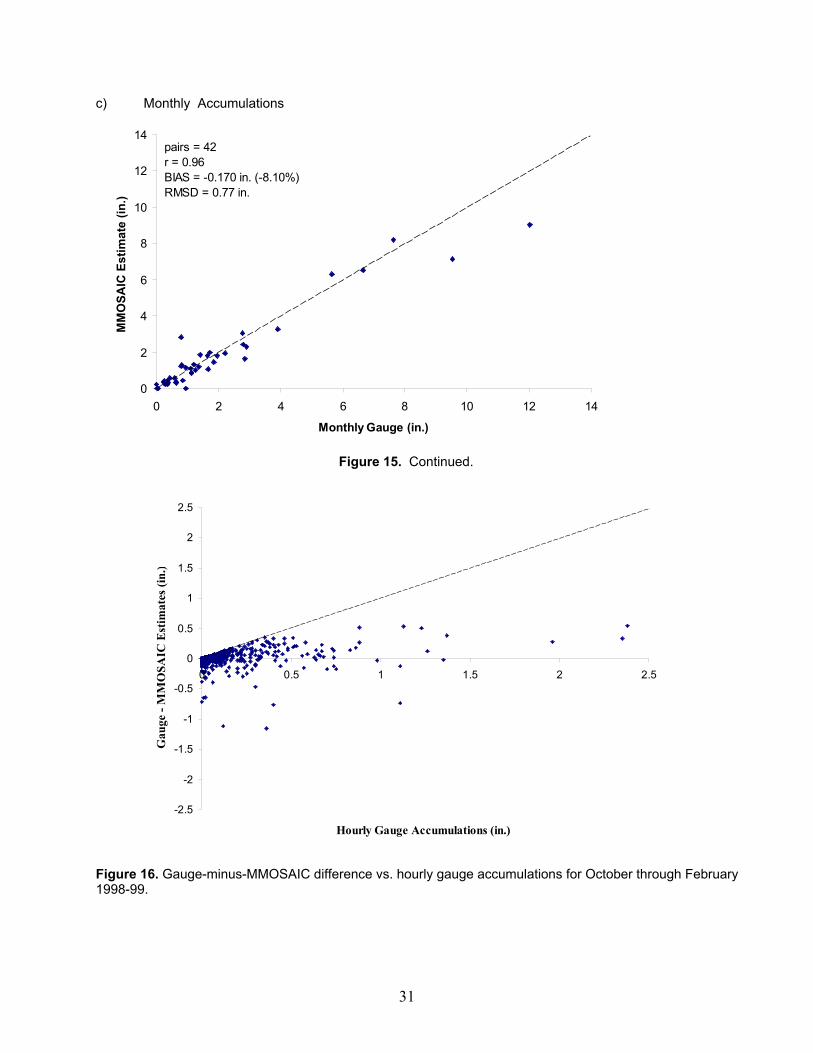
31


0

2

4

6

8

10

12

14

0 2 4 6 8 10 12 14

Monthly Gauge (in.)

MM

OSA

IC E

stim

ate

(in.)



Figure 16. Gauge-minus-MMOSAIC difference vs. hourly gauge accumulations for October through February1998-99.

-2.5

-2

-1.5

-1

-0.5

0

0.5

1

1.5

2

2.5

0 0.5 1 1.5 2 2.5


Gau

ge -

MM

OSA

IC E

stim

ates

(in.

)

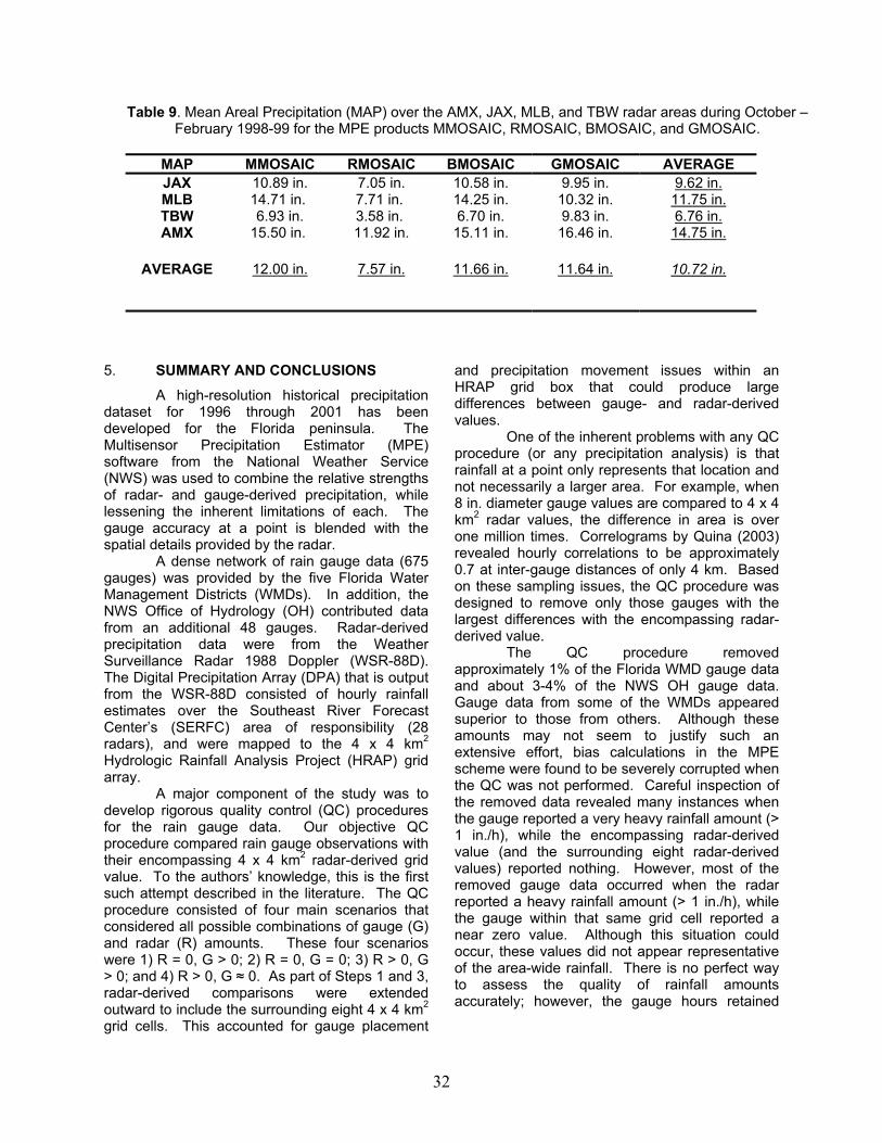
32

Table 9. Mean Areal Precipitation (MAP) over the AMX, JAX, MLB, and TBW radar areas during October –February 1998-99 for the MPE products MMOSAIC, RMOSAIC, BMOSAIC, and GMOSAIC.

MAP MMOSAIC RMOSAIC BMOSAIC GMOSAIC AVERAGEJAX 10.89 in. 7.05 in. 10.58 in. 9.95 in. 9.62 in.MLB 14.71 in. 7.71 in. 14.25 in. 10.32 in. 11.75 in.TBW 6.93 in. 3.58 in. 6.70 in. 9.83 in. 6.76 in.AMX 15.50 in. 11.92 in. 15.11 in. 16.46 in. 14.75 in.


5. SUMMARY AND CONCLUSIONSA high-resolution historical precipitation

dataset for 1996 through 2001 has beendeveloped for the Florida peninsula. TheMultisensor Precipitation Estimator (MPE)software from the National Weather Service(NWS) was used to combine the relative strengthsof radar- and gauge-derived precipitation, whilelessening the inherent limitations of each. Thegauge accuracy at a point is blended with thespatial details provided by the radar. A dense network of rain gauge data (675gauges) was provided by the five Florida WaterManagement Districts (WMDs). In addition, theNWS Office of Hydrology (OH) contributed datafrom an additional 48 gauges. Radar-derivedprecipitation data were from the WeatherSurveillance Radar 1988 Doppler (WSR-88D).The Digital Precipitation Array (DPA) that is outputfrom the WSR-88D consisted of hourly rainfallestimates over the Southeast River ForecastCenter’s (SERFC) area of responsibility (28radars), and were mapped to the 4 x 4 km2

Hydrologic Rainfall Analysis Project (HRAP) gridarray.

A major component of the study was todevelop rigorous quality control (QC) proceduresfor the rain gauge data. Our objective QCprocedure compared rain gauge observations withtheir encompassing 4 x 4 km2 radar-derived gridvalue. To the authors’ knowledge, this is the firstsuch attempt described in the literature. The QCprocedure consisted of four main scenarios thatconsidered all possible combinations of gauge (G)and radar (R) amounts. These four scenarioswere 1) R = 0, G > 0; 2) R = 0, G = 0; 3) R > 0, G> 0; and 4) R > 0, G ≈ 0. As part of Steps 1 and 3,radar-derived comparisons were extendedoutward to include the surrounding eight 4 x 4 km2

grid cells. This accounted for gauge placement

and precipitation movement issues within anHRAP grid box that could produce largedifferences between gauge- and radar-derivedvalues.

One of the inherent problems with any QCprocedure (or any precipitation analysis) is thatrainfall at a point only represents that location andnot necessarily a larger area. For example, when8 in. diameter gauge values are compared to 4 x 4km2 radar values, the difference in area is overone million times. Correlograms by Quina (2003)revealed hourly correlations to be approximately0.7 at inter-gauge distances of only 4 km. Basedon these sampling issues, the QC procedure wasdesigned to remove only those gauges with thelargest differences with the encompassing radar-derived value.

The QC procedure removedapproximately 1% of the Florida WMD gauge dataand about 3-4% of the NWS OH gauge data.Gauge data from some of the WMDs appearedsuperior to those from others. Although theseamounts may not seem to justify such anextensive effort, bias calculations in the MPEscheme were found to be severely corrupted whenthe QC was not performed. Careful inspection ofthe removed data revealed many instances whenthe gauge reported a very heavy rainfall amount (>1 in./h), while the encompassing radar-derivedvalue (and the surrounding eight radar-derivedvalues) reported nothing. However, most of theremoved gauge data occurred when the radarreported a heavy rainfall amount (> 1 in./h), whilethe gauge within that same grid cell reported anear zero value. Although this situation couldoccur, these values did not appear representativeof the area-wide rainfall. There is no perfect wayto assess the quality of rainfall amountsaccurately; however, the gauge hours retained

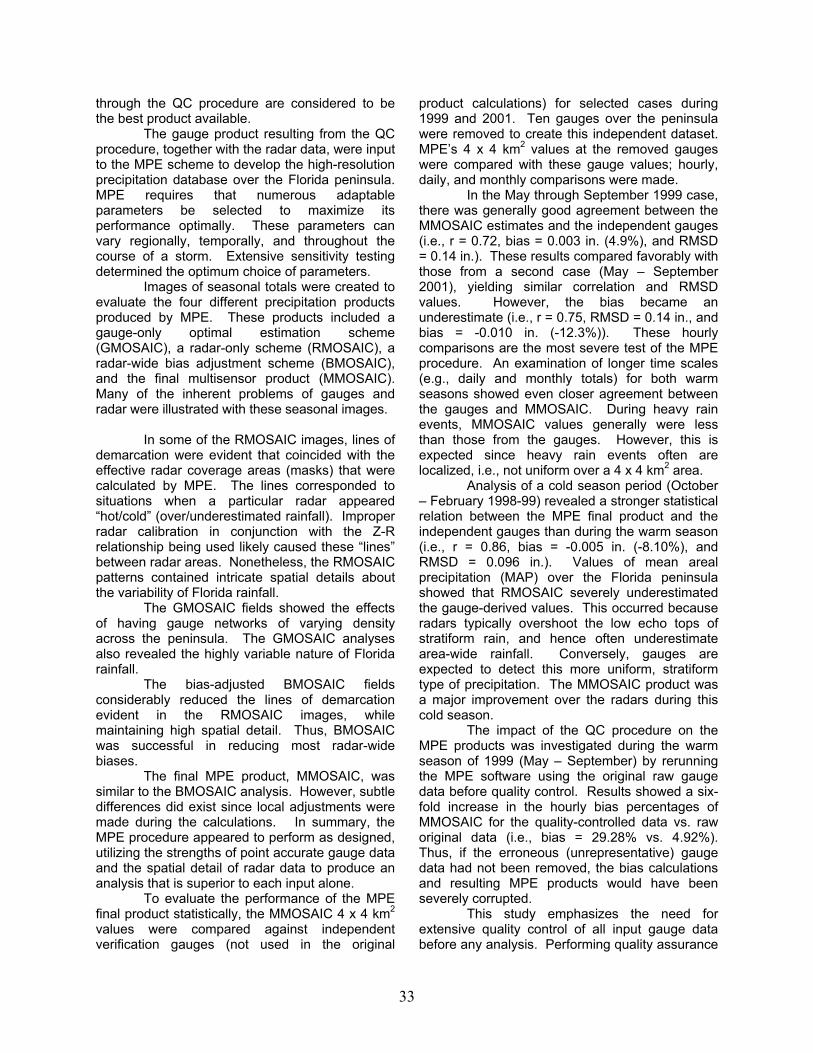
33

through the QC procedure are considered to bethe best product available.

The gauge product resulting from the QCprocedure, together with the radar data, were inputto the MPE scheme to develop the high-resolutionprecipitation database over the Florida peninsula.MPE requires that numerous adaptableparameters be selected to maximize itsperformance optimally. These parameters canvary regionally, temporally, and throughout thecourse of a storm. Extensive sensitivity testingdetermined the optimum choice of parameters.

Images of seasonal totals were created toevaluate the four different precipitation productsproduced by MPE. These products included agauge-only optimal estimation scheme(GMOSAIC), a radar-only scheme (RMOSAIC), aradar-wide bias adjustment scheme (BMOSAIC),and the final multisensor product (MMOSAIC).Many of the inherent problems of gauges andradar were illustrated with these seasonal images.

In some of the RMOSAIC images, lines ofdemarcation were evident that coincided with theeffective radar coverage areas (masks) that werecalculated by MPE. The lines corresponded tosituations when a particular radar appeared“hot/cold” (over/underestimated rainfall). Improperradar calibration in conjunction with the Z-Rrelationship being used likely caused these “lines”between radar areas. Nonetheless, the RMOSAICpatterns contained intricate spatial details aboutthe variability of Florida rainfall.

The GMOSAIC fields showed the effectsof having gauge networks of varying densityacross the peninsula. The GMOSAIC analysesalso revealed the highly variable nature of Floridarainfall.

The bias-adjusted BMOSAIC fieldsconsiderably reduced the lines of demarcationevident in the RMOSAIC images, whilemaintaining high spatial detail. Thus, BMOSAICwas successful in reducing most radar-widebiases.

The final MPE product, MMOSAIC, wassimilar to the BMOSAIC analysis. However, subtledifferences did exist since local adjustments weremade during the calculations. In summary, theMPE procedure appeared to perform as designed,utilizing the strengths of point accurate gauge dataand the spatial detail of radar data to produce ananalysis that is superior to each input alone.

To evaluate the performance of the MPEfinal product statistically, the MMOSAIC 4 x 4 km2

values were compared against independentverification gauges (not used in the original

product calculations) for selected cases during1999 and 2001. Ten gauges over the peninsulawere removed to create this independent dataset.MPE’s 4 x 4 km2 values at the removed gaugeswere compared with these gauge values; hourly,daily, and monthly comparisons were made.

In the May through September 1999 case,there was generally good agreement between theMMOSAIC estimates and the independent gauges(i.e., r = 0.72, bias = 0.003 in. (4.9%), and RMSD= 0.14 in.). These results compared favorably withthose from a second case (May – September2001), yielding similar correlation and RMSDvalues. However, the bias became anunderestimate (i.e., r = 0.75, RMSD = 0.14 in., andbias = -0.010 in. (-12.3%)). These hourlycomparisons are the most severe test of the MPEprocedure. An examination of longer time scales(e.g., daily and monthly totals) for both warmseasons showed even closer agreement betweenthe gauges and MMOSAIC. During heavy rainevents, MMOSAIC values generally were lessthan those from the gauges. However, this isexpected since heavy rain events often arelocalized, i.e., not uniform over a 4 x 4 km2 area.

Analysis of a cold season period (October– February 1998-99) revealed a stronger statisticalrelation between the MPE final product and theindependent gauges than during the warm season(i.e., r = 0.86, bias = -0.005 in. (-8.10%), andRMSD = 0.096 in.). Values of mean arealprecipitation (MAP) over the Florida peninsulashowed that RMOSAIC severely underestimatedthe gauge-derived values. This occurred becauseradars typically overshoot the low echo tops ofstratiform rain, and hence often underestimatearea-wide rainfall. Conversely, gauges areexpected to detect this more uniform, stratiformtype of precipitation. The MMOSAIC product wasa major improvement over the radars during thiscold season.

The impact of the QC procedure on theMPE products was investigated during the warmseason of 1999 (May – September) by rerunningthe MPE software using the original raw gaugedata before quality control. Results showed a six-fold increase in the hourly bias percentages ofMMOSAIC for the quality-controlled data vs. raworiginal data (i.e., bias = 29.28% vs. 4.92%).Thus, if the erroneous (unrepresentative) gaugedata had not been removed, the bias calculationsand resulting MPE products would have beenseverely corrupted.

This study emphasizes the need forextensive quality control of all input gauge databefore any analysis. Performing quality assurance

34

on input data will ensure maximum efficiency ofthe MPE procedure. The objective QC proceduredescribed here is not a perfect scheme; however,it appears to detect those gauges that are mostlikely erroneous. As noted by Steiner et al. (1999),quality control of all data is the single mostimportant step of any precipitation analysis.Although MPE is state of the art software, qualityinput data must be provided to ensure success!

Further research on this high-resolutionhistorical rainfall dataset will extend the coverageto North Florida and the panhandle and to thoseparts of Georgia and Alabama whose watersultimately pass through North Florida. The periodof record will be extended through 2004. Inaddition, we beginning to use the dataset invarious hydrologic studies of the area.

ACKNOWLEDGEMENTS

This project was funded in part by aSection 106 Water Pollution Control Programgrant from the U.S. Environmental ProtectionAgency (US EPA) through Contract WM849 withthe Bureau of Watershed Management of theFlorida Department of Environmental Protection(FDEP). We appreciate the assistance of Mr.Douglas Gilbert and Dr. T.S. Wu of the FDEP inconducting this research. Collaborations with thevarious National Weather Service organizationswere fostered by the NOAA CSTAR grantNA03NWS4680018.

Special appreciation goes to Joel Lanierand Irv Watson of the Tallahassee NationalWeather Service Office for their advice and insightin many discussions about data quality. From theSoutheast River Forecast Center, we would like toespecially thank Judi Bradberry for her time andprompt responses to all of our inquiries. A sincerethanks also to Dongjun Seo and ChandraKondragunta at the Office of Hydrology for theirguidance in QC issues. Jay Breidenbach, formerlyof the Office of Hydrology, provided valuableadvice during early stages of the research. A trulygrateful appreciation goes to Greg Quina for hisvaluable insight and support throughout thisresearch.

REFERENCES

Anagnostou, E. N., and W. F. Krajewski, 1998: Calibration of the WSR-88D PrecipitationProcessing Subsystem. Wea. Forecasting,13, 396-406.

Austin, P. M., 1981: On deducing rainfall from radar reflectivity measurements. Preprints,20th Conference on Radar Meteorology,Boston, MA, Amer. Meteor. Soc., 200-207.

_______, 1987: Relation between measured radar

reflectivity and surface rainfall. Mon. Wea.Rev., 115, 1053-1070.

Baeck, M. L., and J. Smith, 1998: Rainfall estimates by the WSR-88D for heavyrainfall events. Wea. Forecasting, 13, 416-436.

Brandes, E. A., 1975: Optimizing rainfall estimateswith the aid of radar. J. Appl. Meteor., 14,1339-1345.

Breidenbach, J.P., and J. S. Bradberry, 2001. Multisensor precipitation estimatesproduced by National Weather ServiceRiver Forecast Centers for hydrologicapplications. Proceedings 2001 GeorgiaWater Res. Conf., Institute of Ecology,Univ. of Georgia, Athens.

Doviak, R. J., 1983: A survey of radar rain measurement techniques. J. Climate Appl.Meteor., 22, 832-849.

_______, and D. Zrnic, 1993: Doppler Radar and Weather Observations, Second Edition.Academic Press, 562 pp.

Fo, A. J.P., K.C. Crawford, and C.L. Hartzell, 1998: Improving WSR-88D hourly rainfallestimates. Wea. Forecasting, 13, 1016-1028.

Fulton, R. A., J. P. Breidenbach, D.- J. Seo, D. A. Miller, and T. O'Bannon, 1998: The WSR-88D rainfall algorithm. Wea. Forecasting,13, 377-395.

Huff, F. A., 1967: The adjustment of radar estimates of storm mean rainfall with raingage data. J. Appl. Meteor., 6, 52-56.

Hydrology Laboratory, cited 2000: Precipitation truncation problem in the WSR-88D PPSalgorithm: description, quantification andramifications. [available online athttp://www.nws.noaa.gov/oh/hrl/papers/2000mou/MOU00/mou01.html.]

35

_______, cited 2002: Statistical evaluation of "simple fix with filter" solution to theprecipitation truncation problem. [availableonline athttp://www.nws.noaa.gov/oh/hrl/papers/2002mou/chapter-1.pdf.]

Klazura, G. E., J. M. Thomale, D. S. Kelly, and P. Jendrowski, 1999: A comparison ofNEXRAD WSR-88D radar estimates ofrain accumulation with gaugemeasurements for high – and low-reflectivity horizontal gradient precipitationevents. J. Atmos. Oceanic Tech, 16, 1842-1850.

Mroczka, B.A, 2002: The influence of the synoptic flow on warm season rainfall patterns overthe Florida peninsula. M.Sc. Thesis, Dept.Meteorology. The Florida State University(unpublished).

O’Bannon, T., 1998: The WSR-88D rainfallalgorithm. Wea. Forecasting, 13, 377-395.

Quina, G.S. III, 2003: Statistical and hydrological evaluations of rain gauge- and radar-derived precipitation for the Floridapeninsula. M.Sc. Thesis, Dept.Meteorology. The Florida State University(unpublished).

Seed, A., and G. L. Austin, 1990: Variability of summer Florida rainfall and its significancefor the estimation of rainfall by gages,radar, and satellite. J. Geophys. Res., 95,2207-2215.

Seo, D. J., 1998a: Real-time estimation of rainfall fields using rain gauge data underfractional coverage conditions. J. Hydrol.,208, 25-36.

_______, 1998b: Real-time estimation of rainfall fields using radar rainfall and rain gaugedata. J. Hydrol., 208, 37-52.

_______, J. P. Breidenbach, and E. R. Johnson,

1999: Real-time estimation of mean fieldbias in radar rainfall data. J. Hydrol., 223,131-147.

_______, and J. P. Breidenbach, 2002: Real-time correction of spatially nonuniform bias inradar rainfall data using rain gaugemeasurements. J. Hydrometeor., 3, 93-111.

Smith, C. J., 1986: The reduction of errors caused by bright bands in quantitative rainfallmeasurements made using radar. J.Atmos. Oceanic Tech, 3, 129-141.

Smith, J. A. and W. F. Krajewski, 1991: Estimation

of the mean field bias of radar rainfallestimates. J. Appl. Meteor., 30, 397-412.

Steiner, M., J. A. Smith, S. J. Burges, C. V. Alonso, and R. W. Darden, 1999: Effect ofbias adjustment and rain gauge dataquality control on radar rainfall estimation.Water Resour. Res., 35, 2487-2503.

Tollerud, E. I., cited 2000: FSL Forum – Gauge resolution effects on precipitation analysis.[available online athttp://www.fsl.noaa.gov/~vondaust/f200/f300d.html.]

Wilson, J.W., and E.A. Brandes, 1979: Radar measurements of rainfall- A summary.Bull. Amer. Meteor. Soc., 60, 1048-1058.

Woodley, W.L., A.R. Olsen, A. Herndon and V. Wiggert, 1975: Comparison of gage andradar methods of convective rainmeasurement. J. Appl. Meteor., 14, 909-928.

Young, C. B., A. Bradley, W. Krajewski, A. Kruger,

and M. Morrissey, 2000: EvaluatingNEXRAD multisensor precipitationestimates for operational hydrologicforecasting. J. Hydrometeor., 1: 241- 254.

J9.2 DEVELOPING A HIGH RESOLUTION PRECIPITATION … · The South Florida Water Management District...

Documents

Transcript of J9.2 DEVELOPING A HIGH RESOLUTION PRECIPITATION … · The South Florida Water Management District...