J S I A Mjsiaml.jsiam.org/ebooks/JSIAMLetters_vol5-2013.pdf · Takuya Tsuchiya (Ehime University)...
76
J S I A M The Japan Society for Industrial and Applied Mathematics Vol.5 (2013) pp.1-68
Transcript of J S I A Mjsiaml.jsiam.org/ebooks/JSIAMLetters_vol5-2013.pdf · Takuya Tsuchiya (Ehime University)...

J S I A M
The Japan Society for Industrial and Applied Mathematics
Vol.5 (2013) pp.1-68


The Japan Society for Industrial and Applied Mathematics
Vol.5 (2013) pp.1-68

Editorial Board
Chief Editor Hideyuki Azegami (Nagoya University)
Vice-Chief Editor Yoshimasa Nakamura (Kyoto University)
Secretary Editors Ken'ichiro Tanaka (Future University Hakodate)
Kenji Shirota (Aichi Prefectural University)
Tomohiro Sogabe (Aichi Prefectural University)
Associate Editors Kazuo Kishimoto (Tsukuba University)
Reiji Suda (University of Tokyo)
Satoshi Tsujimoto (Kyoto University)
Masashi Iwasaki (Kyoto Prefectural University)
Norikazu Saito (University of Tokyo)
Koh-ichi Nagao (Kanto Gakuin University)
Koichi Kato (Japan Institute for Pacific Studies)
Nagai Atsushi (Nihon University)
Takeshi Mandai (Osaka Electro-Communication University)
Kiyoshi Mizohata (Doshisha University)
Tamotu Kinoshita (University of Tsukuba)
Yuzuru Sato (Hokkaido University)
Ken Umeno (Kyoto University)
Kazuyuki Yoshimura (NTT Communication Science Laboratories)
Katsuhiro Nishinari (University of Tokyo)
Tetsu Yajima (Utsunomiya University)
Narimasa Sasa (Japan Atomic Energy Agency)
Fumiko Sugiyama (Kyoto University)
Jun Mitani (University of Tsukuba)
Hitoshi Imai (University of Tokushima)
Takuya Tsuchiya (Ehime University)
Daisuke Furihata (Osaka University)
Takayasu Matsuo (Tokyo University)
Hiroto Tadano (University of Tsukuba)
Takafumi Miyata (Nagoya University
Ken Hayami (National Institute of Informatics)
Kensuke Aishima (University of Tokyo)
Yoshitaka Watanabe (Kyushu University)
Katsuhisa Ozaki (Shibaura Institute of Technology)
Naoya Yamanaka (Waseda University)
Takaaki Nara (University of Electro-Communications)
Takashi Suzuki (Osaka University)
Tetsuo Ichimori (Osaka Institute of Technology)
Tatsuo Oyama (National Graduate Institute for Policy Studies)
Eiji Katamine (Gifu National College of Technology)
Junichi Matsumoto (National Institute of Advanced Industrial Science and Technology)
Mitsuharu Yamamoto (Chiba University)
Maki Yoshida (Osaka University)
Hideki Sakurada (NTT Communication Science Laboratories)
Naoyuki Ishimura (Hitotsubashi University)

Jiro Akahori (Ritsumeikan University)
Kiyomasa Narita (Kanagawa University)
Ken Nakamura (Tokyo Metropolitan University)
Toru Komatsu (Tokyo University of Science)
Kazuto Matsuo (Kanagawa University)
Hiroshi Kawaharada (Chuo University)
Ichiro Kataoka (Hitachi)
Naoshi Nishimura (Kyoto University)
Hiromichi Itou (Tokyo University of Science)
Shuji Kijima (Kyushu University)
Akiyoshi Shioura (Tohoku University)
Takeshi Ogita (Tokyo Woman's Christian University)
Maho Nakata (Riken)
Takaharu Yaguchi (Kobe University)

Contents
A note on the Sinc approximationwith boundary treatment ・・・ 1-4
Tomoaki Okayama
Remarks on numerical integration of L1 norm ・・・ 5-8
Takahito Kashiwabara, Issei Oikawa
Development and acceleration of multiple precision arithmetic toolbox MuPAT for
Scilab ・・・ 9-12
Satoko Kikkawa, Tsubasa Saito, Emiko Ishiwata, Hidehiko Hasegawa
Remarks on the rate of strong convergence of Euler-Maruyama approximation for SDEs
driven by rotation invariant stable processes ・・・ 13-16
Hiroya Hashimoto, Takahiro Tsuchiya
An asymptotic expansion formula for up-and-out barrier option price under stochastic
volatility model ・・・ 17-20
Takashi Kato, Akihiko Takahashi, Toshihiro Yamada
An application of the Kato-Temple inequality on matrix eigenvalues to the dqds
algorithm for singular values ・・・ 21-24
Takumi Yamashita, Kinji Kimura, Masami Takata, Yoshimasa Nakamura
Convergence analysis of accurate inverse Cholesky factorization ・・・ 25-28
Yuka Yanagisawa, Takeshi Ogita
Error analysis of the H1 gradient method for shape-optimization problems of continua ・・・ 29-32
Daisuke Murai, Hideyuki Azegami
Complete low-cut filter and the best constant of Sobolev inequality ・・・ 33-36
Hiroyuki Yamagishi, Yoshinori Kametaka, Atsushi Nagai, Kohtaro Watanabe, Kazuo Takemura
A new geometric integration approach based on local invariants ・・・ 37-40
Takeru Matsuda, Takayasu Matsuo
A projection method for nonlinear eigenvalue problems using contour integrals ・・・ 41-44
Shinnosuke Yokota, Tetsuya Sakurai
Improvement of key generation for a number field based knapsack cryptosystem ・・・ 45-48
Yasunori Miyamoto, Ken Nakamula
Improvement of multiple kernel learning using adaptively weighted regularization ・・・ 49-52
Taiji Suzuki
The best estimation corresponding to continuous model of Thomson cable ・・・ 53-56
Hiroyuki Yamagishi, Yoshinori Kametaka, Atsushi Nagai, Kohtaro Watanabe, Kazuo Takemura
A new method for fast computation of cumulative distribution functions by fractional
FFT ・・・ 57-60
Ken'ichiro Tanaka
Construction method of the cost function for the minimax shape optimization problem ・・・ 61-64
Kouhei Shintani, Hideyuki Azegami
A Weighted Block GMRES method for solving linear systems with multiple right-hand
sides ・・・ 65-68
Akira Imakura, Lei Du, Hiroto Tadano

JSIAM Letters Vol.5 (2013) pp.1–4 c⃝2013 Japan Society for Industrial and Applied Mathematics J S I A MLetters
A note on the Sinc approximation
with boundary treatment
Tomoaki Okayama1
1 Graduate School of Economics, Hitotsubashi University, 2-1, Naka, Kunitachi, Tokyo 186-8601, Japan
E-mail tokayama econ.hit-u.ac.jp
Received April 23, 2012, Accepted June 27, 2012
Abstract
The original form of the Sinc approximation is efficient for functions whose boundary valuesare zero, but not for other functions. The typical way to treat general boundary values is tointroduce auxiliary basis functions, and in fact such an approach has been taken commonly inthe literature. However, the approximation formula in each research is not exactly the same,and still other formulas can be derived as variants of existing formulas. The purpose of thispaper is to sum up those existing formulas and new ones, and to give explicit proofs of thoseconvergence theorems.
Keywords Sinc approximation, Sinc-collocation, boundary treatment
Research Activity Group Scientific Computation and Numerical Analysis
1. Variants of the Sinc approximation
The Sinc approximation on the real axis is expressedas
F (x) ≈N∑
j=−M
F (jh)S(j, h)(x), x ∈ R, (1)
where S(j, h)(x) is the so-called Sinc function defined byS(j, h)(x) = sin(π(x/h − j))/[π(x/h − j)], and h,M,Nare suitably selected with respect to n. The approxima-tion (1) requires two conditions on F :
(i) F must be defined on the entire real axis, and
(ii) F (x) must tend to zero as x→ ±∞.
There is a typical remedy for the first condition (i). Ifwe consider the approximation of f that is defined onlyon the finite interval Γ = (a, b), choose a proper variabletransformation ψ that maps R onto Γ , then put F (x) =f(ψ(x)) and use (1). The standard transformation is
t = ψSE(x) =b− a2
tanh(x2
)+b+ a
2,
which is called the Single-Exponential (SE) transforma-tion, and the explicit approximation form is:
f(t) ≈N∑
j=−Mf(tSEj )S(j, h)(ϕSE(t)), t ∈ Γ, (2)
where tSEj = ψSE(jh) and ϕSE(t) = ψSE−1(t). The for-mula (2) is called the SE-Sinc approximation.The condition (ii) still remains; f(a) = f(b) = 0 is
required in (2). The common remedy is to construct afunction with zero boundary values by the operator T :
T [f ](t) = f(t)− f(a)Wa(t)− f(b)Wb(t),
where Wa and Wb are auxiliary basis functions definedby Wa(t) = (b− t)/(b−a), Wb(t) = (t−a)/(b−a). Then
T f can be approximated by (2). The explicit form is:
f(t) ≈ f(a)Wa(t) + f(b)Wb(t)
+
N∑j=−M
T [f ](tSEj )S(j, h)(ϕSE(t)). (3)
This formula has been used by some authors for derivingSinc-collocation methods for differential/integral equa-tions [1–3]. However, the interpolating points of (3) arenot consistent: t = a, tSE−M , t
SE−M+1, . . . , t
SEN , b, which have
two exceptions (t = a and t = b). These exceptions makeimplementation more complicated, especially in the casethat the target is a system of many equations.In order to correct the defect, the following formula:
f(t) ≈ f(tSE−M )Wa(t) + f(tSEN )Wb(t)
+N∑
j=−M
T SE[f ](tSEj )S(j, h)(ϕSE(t)) (4)
has been used [4, § 6–7], where
T SE[f ](t) = f(t)− f(tSE−M )Wa(t)− f(tSEN )Wb(t).
This formula works fine since f(a) ≈ f(tSE−M ) and f(b) ≈f(tSEN ), and the interpolating points are consistent andsimple: t = tSE−M , . . . , t
SEN .
Similar, but different, another formula with the simpleinterpolating points has been proposed [5]:
f(t) ≈ fa(tSE−M )Wa(t) + fb(tSEN )Wb(t)
+N∑
j=−M
T SE[f ](tSEj )S(j, h)(ϕSE(t)), (5)
where fa(t) = f(t)/Wa(t), fb(t) = f(t)/Wb(t), and
T SE[f ](t) = f(t)− fa(tSE−M )Wa(t)− fb(tSEN )Wb(t).
– 1 –

JSIAM Letters Vol. 5 (2013) pp.1–4 Tomoaki Okayama
Stenger [5] has introduced the following notations:
ωSE−M (x) =
(1 + ρSE(−Mh)
)( 1
1 + ρSE(x)
−N∑
k=−M+1
1
1 + ρSE(kh)S(k, h)(x)
),
ωSEj (x) = S(j, h)(x), −M < j < N,
ωSEN (x) =
1 + ρSE(Nh)
ρSE(Nh)
(ρSE(x)
1 + ρSE(x)
−N−1∑k=−M
ρSE(kh)
1 + ρSE(kh)S(k, h)(x)
),
where ρSE(x) = ex. Then (5) can be rewritten as
f(t) ≈N∑
j=−M
f(tSEj )ωSEj (ϕSE(t)).
In this form we easily see the interpolating points sinceωSEj (ih) = δij . The formulas through (3)–(5) should be
called generalized SE-Sinc approximations in the sensethat they can handle general boundary values. The firstpurpose of this paper is to sum up convergence theoremsof the formulas with proofs (not explicitly given so far).If we return our attention to the condition (i), there
is another famous variable transformation:
t = ψDE(x) =b− a2
tanh(π2sinhx
)+b+ a
2,
which is called the Double-Exponential (DE) transfor-mation. This transformation also maps R onto Γ , andwe can consider the DE-Sinc approximation by replac-ing ‘SE’ with ‘DE’ in (2). Accordingly the formula (3)can be modified as
f(t) ≈ f(a)Wa(t) + f(b)Wb(t)
+N∑
j=−M
T [f ](tDEj )S(j, h)(ϕDE(t)), (6)
and in fact this formula has also been used [2, 3] as ageneralized DE-Sinc approximation. In addition, we canderive two new generalized DE-Sinc approximations:
f(t) ≈ f(tDE−M )Wa(t) + f(tDE
N )Wb(t)
+N∑
j=−M
T DE[f ](tDEj )S(j, h)(ϕDE(t)), (7)
f(t) ≈ fa(tDE−M )Wa(t) + fb(t
DEN )Wb(t)
+N∑
j=−M
T DE[f ](tDEj )S(j, h)(ϕDE(t)), (8)
by replacing ‘SE’ with ‘DE’ in (4) and (5), respectively.If we define ρDE as ρDE(x) = eπ sinh x, and replace ‘SE’with ‘DE’ in Stenger’s notations, the latter formula (8)can be rewritten as
f(t) ≈N∑
j=−Mf(tDE
j )ωDEj (ϕDE(t)).
In addition to deriving (7) and (8) for simple interpolat-ing points, this paper gives explicit proofs of the conver-gence theorems for (6)–(8), which is the second purpose.This paper is organized as follows. The convergence
theorems for (3)–(8) are stated in Section 2, and it turnsout the convergence rate of the formulas (3)–(5) is thesame, O(
√n e−c
√n). The convergence rate of the formu-
las (6)–(8) is also the same: O( e−c′n/ logn), but much
higher than SE’s rate. The result is confirmed numeri-cally in Section 3. Section 4 is devoted to proofs.
2. Convergence theorems
The following function space is crucial in this section.
Definition 1 Let D be a bounded and simply-connecteddomain (or Riemann surface) that contains the intervalΓ . Let α and β be positive constants with α ≤ 1 andβ ≤ 1. Then Mα,β(D) denotes the family of all functionsf that are analytic and bounded on D , and satisfy thefollowing inequalities with a constant C:
|f(z)− f(a)| ≤ C|z − a|α,
|f(b)− f(z)| ≤ C|b− z|β ,
for all z ∈ D .
In the subsequent theorems, D is either ψSE(Dd) orψDE(Dd), where Dd = ζ ∈ C : | Im ζ| < d for d > 0.
Let us define ϵSEn and ϵDEn as ϵSEn =
√n e−
√πdµn and
ϵDEn = e−πdn/ log(2dn/µ) for short.First three theorems are for the formula (3)–(5).
Theorem 2 (Well-known, cf. Stenger [4, §4])Let f ∈ Mα,β(ψ
SE(Dd)) for d ∈ (0, π). Letµ = minα, β, n be a positive integer, and h beselected by the formula
h =
√πd
µn. (9)
Moreover, let M and N be positive integers defined byM = n, N = ⌈αn/β⌉ (if µ = α)N = n, M = ⌈βn/α⌉ (if µ = β)
(10)
respectively. Then there exists a constant C independentof n such that
supt∈Γ
∣∣∣∣∣T [f ](t)−N∑
j=−M
T [f ](tSEj )S(j, h)(ϕSE(t))
∣∣∣∣∣ ≤ CϵSEn .
Theorem 3 Let the assumptions in Theorem 2 be ful-filled. Then there exists a constant C independent of nsuch that
supt∈Γ
∣∣∣∣∣T SE[f ](t)−N∑
j=−M
T SE[f ](tSEj )S(j, h)(ϕSE(t))
∣∣∣∣∣≤ CϵSEn .
Theorem 4 (Stenger [5, Theorem 4.2]) Let theassumptions in Theorem 2 be fulfilled. Then there existsa constant C independent of n such that
supt∈Γ
∣∣∣∣∣f(t)−N∑
j=−M
f(tSEj )ωSEj (ϕSE(t))
∣∣∣∣∣ ≤ CϵSEn .
– 2 –
JSIAM Letters Vol. 5 (2013) pp.1–4 Tomoaki Okayama
The following three theorems are for (6)–(8).
Theorem 5 Let f ∈Mα,β(ψDE(Dd)) for d ∈ (0, π/2).
Let µ = minα, β, n be a positive integer, and h beselected by the formula
h =log(2dn/µ)
n. (11)
Moreover, let M and N be positive integers defined byM = n, N = n− ⌊log(β/α)/h⌋ (if µ = α)N = n, M = n− ⌊log(α/β)/h⌋ (if µ = β)
(12)
respectively. Then there exists a constant C independentof n such that
supt∈Γ
∣∣∣∣∣T [f ](t)−N∑
j=−MT [f ](tDE
j )S(j, h)(ϕDE(t))
∣∣∣∣∣ ≤ CϵDEn .
Theorem 6 Let the assumptions in Theorem 5 be ful-filled. Then there exists a constant C independent of nsuch that
supt∈Γ
∣∣∣∣∣T DE[f ](t)−N∑
j=−MT DE[f ](tDE
j )S(j, h)(ϕDE(t))
∣∣∣∣∣≤ CϵDE
n .
Theorem 7 Let the assumptions in Theorem 5 be ful-filled. Then there exists a constant C independent of nsuch that
supt∈Γ
∣∣∣∣∣f(t)−N∑
j=−Mf(tDE
j )ωDEj (ϕDE(t))
∣∣∣∣∣ ≤ CϵDEn .
3. Numerical results
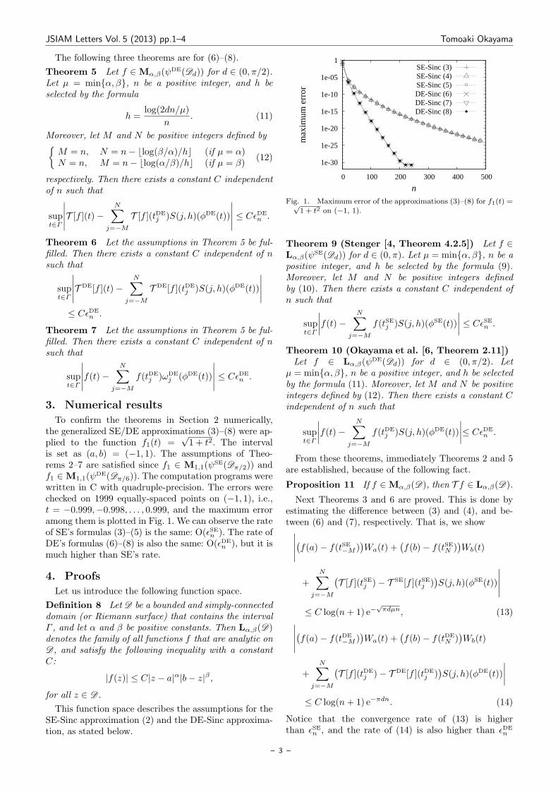
To confirm the theorems in Section 2 numerically,the generalized SE/DE approximations (3)–(8) were ap-plied to the function f1(t) =
√1 + t2. The interval
is set as (a, b) = (−1, 1). The assumptions of Theo-rems 2–7 are satisfied since f1 ∈ M1,1(ψ
SE(Dπ/2)) andf1 ∈M1,1(ψ
DE(Dπ/6)). The computation programs werewritten in C with quadruple-precision. The errors werechecked on 1999 equally-spaced points on (−1, 1), i.e.,t = −0.999,−0.998, . . . , 0.999, and the maximum erroramong them is plotted in Fig. 1. We can observe the rateof SE’s formulas (3)–(5) is the same: O(ϵSEn ). The rate ofDE’s formulas (6)–(8) is also the same: O(ϵDE
n ), but it ismuch higher than SE’s rate.
4. Proofs
Let us introduce the following function space.
Definition 8 Let D be a bounded and simply-connecteddomain (or Riemann surface) that contains the intervalΓ , and let α and β be positive constants. Then Lα,β(D)denotes the family of all functions f that are analytic onD , and satisfy the following inequality with a constantC:
|f(z)| ≤ C|z − a|α|b− z|β ,
for all z ∈ D .
This function space describes the assumptions for theSE-Sinc approximation (2) and the DE-Sinc approxima-tion, as stated below.
1e-30
1e-25
1e-20
1e-15
1e-10
1e-05
1
0 100 200 300 400 500
max
imum
err
or
n
SE-Sinc (3)SE-Sinc (4)SE-Sinc (5)DE-Sinc (6)DE-Sinc (7)DE-Sinc (8)
Fig. 1. Maximum error of the approximations (3)–(8) for f1(t) =√1 + t2 on (−1, 1).
Theorem 9 (Stenger [4, Theorem 4.2.5]) Let f ∈Lα,β(ψ
SE(Dd)) for d ∈ (0, π). Let µ = minα, β, n be apositive integer, and h be selected by the formula (9).Moreover, let M and N be positive integers definedby (10). Then there exists a constant C independent ofn such that
supt∈Γ
∣∣∣∣f(t)− N∑j=−M
f(tSEj )S(j, h)(ϕSE(t))
∣∣∣∣ ≤ CϵSEn .
Theorem 10 (Okayama et al. [6, Theorem 2.11])Let f ∈ Lα,β(ψ
DE(Dd)) for d ∈ (0, π/2). Letµ = minα, β, n be a positive integer, and h be selectedby the formula (11). Moreover, let M and N be positiveintegers defined by (12). Then there exists a constant Cindependent of n such that
supt∈Γ
∣∣∣∣f(t)− N∑j=−M
f(tDEj )S(j, h)(ϕDE(t))
∣∣∣∣≤ CϵDEn .
From these theorems, immediately Theorems 2 and 5are established, because of the following fact.
Proposition 11 If f ∈Mα,β(D), then T f ∈ Lα,β(D).
Next Theorems 3 and 6 are proved. This is done byestimating the difference between (3) and (4), and be-tween (6) and (7), respectively. That is, we show∣∣∣∣∣(f(a)− f(tSE−M )
)Wa(t) +
(f(b)− f(tSEN )
)Wb(t)
+N∑
j=−M
(T [f ](tSEj )− T SE[f ](tSEj )
)S(j, h)(ϕSE(t))
∣∣∣∣∣≤ C log(n+ 1) e−
√πdµn, (13)∣∣∣∣∣(f(a)− f(tDE
−M ))Wa(t) +
(f(b)− f(tDE
N ))Wb(t)
+
N∑j=−M
(T [f ](tDE
j )− T DE[f ](tDEj ))S(j, h)(ϕDE(t))
∣∣∣∣≤ C log(n+ 1) e−πdn. (14)
Notice that the convergence rate of (13) is higherthan ϵSEn , and the rate of (14) is also higher than ϵDE
n
– 3 –

JSIAM Letters Vol. 5 (2013) pp.1–4 Tomoaki Okayama
(limn→∞ log(n + 1) e−πdn/ϵDEn = 0). From those esti-
mates and the next lemma, Theorems 3 and 6 are proved.
Lemma 12 (Stenger [4, p. 142]) Let h > 0. Then
supx∈R
n∑j=−n
|S(j, h)(x)| ≤ 2
π(3 + log n).
Proof of Theorem 3 From f ∈ Mα,β(ψSE(Dd)), we
have∣∣f(tSE−M )− f(a)∣∣ ≤ C(tSE−M − a)α =
C(b− a)α
(1 + eMh)α,
∣∣f(b)− f(tSEN )∣∣ ≤ C(b− tSEN )β =
C(b− a)β
(1 + eNh)β.
Moreover, using |Wa(t)| ≤ 1 and |Wb(t)| ≤ 1, and sub-stituting (9)–(10), we have the following bound:∣∣(f(a)− f(tSE−M )
)Wa(t) +
(f(b)− f(tSEN )
)Wb(t)
∣∣≤ C1 e
−√πdµn,
for some constant C1. From this we also have∣∣T [f ](tSEj )− T SE[f ](tSEj )∣∣ ≤ C1 e
−√πdµn.
Finally using Lemma 12 we obtain (13).(QED)
Similarly, Theorem 6 can be shown as follows.
Proof of Theorem 6 Since f ∈Mα,β(ψDE(Dd)), we
have∣∣f(tDE−M )− f(a)
∣∣ ≤ C(tDE−M − a)α =
C(b− a)α
(1 + eπ sinh(Mh))α,
∣∣f(b)− f(tDEN )∣∣≤ C(b− tDE
N )β =C(b− a)β
(1 + eπ sinh(Nh))β.
Moreover, using |Wa(t)| ≤ 1 and |Wb(t)| ≤ 1, and sub-stituting (11)–(12), we have the following bound:∣∣(f(a)− f(tDE
−M ))Wa(t) +
(f(b)− f(tDE
N ))Wb(t)
∣∣≤ C2 e
−πdn,
for some constant C2. From this we also have∣∣T [f ](tDEj )− T DE[f ](tDE
j )∣∣≤ C2 e
−πdn.
Finally using Lemma 12 we obtain (14).(QED)
Let us now proceed to Theorems 4 and 7. We will esti-mate the difference between (4) and (5), and between (7)and (8), respectively. That is, we show∣∣∣∣(f(tSE−M )− fa(tSE−M )
)Wa(t) +
(f(tSEN )− fb(tSEN )
)Wb(t)
+N∑
j=−M
(T SE[f ](tSEj )− T SE[f ](tSEj )
)S(j, h)(ϕSE(t))
∣∣∣∣≤ C log(n+ 1) e−
√πdn/ν , (15)∣∣∣∣(f(tDE
−M )− fa(tDE−M )
)Wa(t) +
(f(tDE
N )− fb(tDEN ))Wb(t)
+N∑
j=−M
(T DE[f ](tDE
j )− T DE[f ](tDEj ))S(j, h)(ϕDE(t))
∣∣∣∣≤ C log(n+ 1) e−πdn/ν , (16)
where ν = maxα, β. From these estimates Theorems 4and 7 are proved, since the convergence rate of (15) ishigher than ϵSEn , and the rate of (16) is also higher thanϵDEn (notice −πdn/ν ≤ −πdn since ν ∈ (0, 1]).
Proof of Theorem 4 Firstly we easily have∣∣fa(tSE−M )− f(tSE−M )∣∣ = ∣∣f(tSE−M )
∣∣ e−Mh,∣∣fb(tSEN )− f(tSEN )∣∣ = ∣∣f(tSEN )
∣∣ e−Nh.Moreover, using |Wa(t)| ≤ 1, |Wb(t)| ≤ 1, and α, β ∈(0, 1], and substituting (9)–(10), we have:∣∣(f(tSE−M )− fa(tSE−M )
)Wa(t) +
(f(tSEN )− fb(tSEN )
)Wb(t)
∣∣≤ C1 e
−√πdn/ν ,
for some constant C1. From this we also have∣∣T SE[f ](tSEj )− T SE[f ](tSEj )∣∣ ≤ C1 e
−√πdn/ν .
Finally using Lemma 12 we obtain (15).(QED)
Proof of Theorem 7 Firstly we easily have∣∣fa(tDE−M )− f(tDE
−M )∣∣ = ∣∣f(tDE
−M )∣∣ e−π sinh(Mh),∣∣fb(tDE
N )− f(tDEN )∣∣ = ∣∣f(tDE
N )∣∣ e−π sinh(Nh).
Moreover, using |Wa(t)| ≤ 1, |Wb(t)| ≤ 1, and α, β ∈(0, 1], and substituting (11)–(12), we have:∣∣f(tDE
−M )− fa(tDE−M )Wa(t) + f(tDE
N )− fb(tDEN )Wb(t)
∣∣≤ C1 e
−πdn/ν ,
for some constant C1. From this we also have∣∣T DE[f ](tDEj )− T DE[f ](tDE
j )∣∣ ≤ C1 e
−πdn/ν .
Finally using Lemma 12 we obtain (16).(QED)
Acknowledgments
This work was supported by JSPS Grants-in-Aid forScientific Research.
References
[1] B. Bialecki, Sinc-collocation methods for two-point boundaryvalue problems, IMA J. Numer. Anal., 11 (1991), 357–375.
[2] T. Okayama, T. Matsuo and M. Sugihara, Sinc-collocationmethods for weakly singular Fredholm integral equations ofthe second kind, J. Comput. Appl. Math., 234 (2010), 1211–1227.
[3] T. Okayama, T. Matsuo and M. Sugihara, Improvement ofa Sinc-collocation method for Fredholm integral equations ofthe second kind, BIT Numer. Math., 51 (2011), 339–366.
[4] F. Stenger, Numerical Methods Based on Sinc and Analytic
Functions, Springer-Verlag, New York, 1993.[5] F. Stenger, Collocating convolutions, Math. Comp., 64
(1995), 211–235.[6] T. Okayama, T. Matsuo and M. Sugihara, Error estimates
with explicit constants for Sinc approximation, Sinc quadra-ture and Sinc indefinite integration, Numer. Math., in press.
– 4 –
JSIAM Letters Vol.5 (2013) pp.5–8 c⃝2013 Japan Society for Industrial and Applied Mathematics J S I A MLetters
Remarks on numerical integration of L1 norm
Takahito Kashiwabara1 and Issei Oikawa1
1 Graduate School of Mathematical Sciences, The University of Tokyo, 3-8-1 Komaba, Meguro,Tokyo 153-8914, Japan
E-mail tkashiwa ms.u-tokyo.ac.jp
Received March 7, 2012, Accepted July 23, 2012
Abstract
Non-differentiability of the absolute value function at the origin can affect the accuracy ofnumerical computations for the L1 norm. We present an example in which the accuracy doesdeteriorate, and we provide a convergence order for such situations. We propose a simplealgorithm to improve the convergence order, confirming its effectiveness as in the exampledescribed above. Mesh-dependent integrands and applications to finite element method arealso considered.
Keywords numerical integration, non-smooth integrand, error estimate
Research Activity Group Scientific Computation and Numerical Analysis
1. Introduction
We consider the one-dimensional integral of a contin-uous function f on [a, b], that is,
I(f ; a, b) =
∫ b
a
f(x) dx,
and its approximation as
In(f ; a, b) = (b− a)n∑j=1
wjf(xj), (1)
where wj and xj = (1− tj)a+ tjb, 0 ≤ t1 < · · · < tn ≤ 1denote the weights and integral points respectively. Forexample, Newton–Cotes and Gaussian quadrature rulescan be written with the form shown above (see Table 1).We refer to the exactness of In as r, which implies thatIn is exact for polynomials of degree ≤ r. Throughoutthis paper, the weights are assumed to be positive, i.e.,
wj > 0, j = 1, . . . , n.
Let ∆h : a = a0 < a1 < · · · < aN < aN+1 = b bea mesh of [a, b], with h = max0≤i≤N |ai+1 − ai|. Thecomposite formula based on (1) is defined as
Icn(f ; a, b) =N∑i=0
In(f ; ai, ai+1).
In what follows, we simply write I(f) instead of I(f ; a, b)etc. when there is no possibility of confusion. Conver-gence order estimates for En(f) = In(f) − I(f) andEcn(f) = Icn(f)− I(f) are well known if f is sufficientlysmooth:
Proposition 1 Let In have exactness r ≥ 0.(i) For all f ∈ Cr+1([a, b]),
|E(f ; a, b)| ≤ 2
(r + 1)!(b− a)r+2 max
a≤x≤b|f (r+1)|. (2)
Table 1. Examples of In for n ≤ 3.
Newton–Cotes Gauss
n 1 2 3 2 3
t1 1/2 0 0 (1−√
1/3)/2 (1−√
3/5)/2
t2 – 1 1/2 (1 +√
1/3)/2 1/2
t3 – – 1 – (1 +√
3/5)/2w1 1 1/2 1/6 1/2 5/18
w2 – 1/2 4/6 1/2 8/18w3 – – 1/6 – 5/18
r 1 1 3 3 5
(ii) For all f ∈ Cr+1([a, b]),
|Ecn(f ; a, b)| ≤2(b− a)(r + 1)!
hr+1 maxa≤x≤b
|f (r+1)|.
Proof (i) Let f be a Lagrange interpolation of f withdegree r. Noting that En(f) = In(f − f) + I(f − f)and
∑nj=1 |wj | = 1, we conclude (2) from the standard
interpolation error estimate (e.g. [1, Theorem 8.2])
maxa≤x≤b
|f − f | ≤ 1
(r + 1)!(b− a)r+1 max
a≤x≤b|f (r+1)|.
(ii) Because∑Ni=0(ai+1−ai) = b−a, this is an imme-
diate consequence of (i).(QED)
The estimate presented above, however, is inapplica-ble to a computation of the L1(a, b) norm, i.e. I(|f |) =∫ ba|f(x)| dx because |f(x)| is not differentiable at points
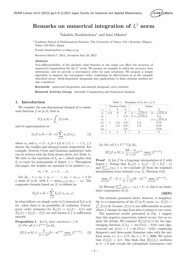
where f changes its sign from plus to minus or vice versa.The numerical results presented in Fig. 1 suggest
that this negative expectation indeed occurs. Let us ex-plain the details. We compute Ecn(|f |; 0, 1) for the sign-changing function f1(x) = sin 17π(x − 0.01) and sign-constant one f2(x) = 1 + sin 17π(x − 0.01), employingSimpson’s and three-point Gaussian rules with the uni-form mesh, i.e. h = 1/N , for 1 ≤ N ≤ 3000. We noticethat I(|f1|) = 2/π. One finds that Ecn(|f1|) oscillatesas h → 0 and reveals the suboptimal convergence rate
– 5 –

JSIAM Letters Vol. 5 (2013) pp.5–8 Takahito Kashiwabara et al.
10-16
10-14
10-12
10-10
10-8
10-6
10-4
10-2
100
100
101
102
103
Err
or
N: Number of intervals
4
2
sin17π(x-0.01)
1+sin17π(x-0.01)
10-16
10-14
10-12
10-10
10-8
10-6
10-4
10-2
100
100
101
102
103
Err
or
N: Number of intervals
6
2
sin17π(x-0.01)
1+sin17π(x-0.01)
Fig. 1. Convergence behavior of Ecn(|f |; 0, 1) for f1 and f2.
(top, Simpson’s rule; bottom, three-point Gaussian rule.)
O(h2), whereas Ecn(|f2|) decreases monotonically at theoptimal rate O(h4) or O(h6) given by Proposition 1.The purpose of this paper is to provide a theoretical
analysis for Ecn(|f |). In Section 2, we establish severalconvergence-order estimates depending on assumptionsrelated to the mesh or regularity of f . Particularly, asufficient condition to recover the optimal order is de-scribed.To achieve that condition, we propose a numerical
implementation in Section 3 using a zero-point searchbased on Newton’s method. Unfortunately, such a strat-egy might not work when the integrand f depends onthe mesh, as discussed in Section 4.Section 5 presents several applications to problems ap-
pearing in finite element method. Finally, we describeperspectives for future works in Section 6.
2. Convergence analysis for Ecn(|f |)
Here and hereinafter we use the standard notation ofLebesgue and Sobolev spaces. The integral points usedin the composite formula Icn are denoted as
xi,j = (1− tj)ai + tjai+1
for i = 0, . . . , N, and j = 1, . . . , n. Therefore, Icn is rep-resented as
Icn(f ; a, b) =
N∑i=0
(ai+1 − ai)n∑j=1
wjf(xi,j).
First, let us prove the O(h) result for Ecn(|f |) underf ∈W 1,1(a, b). This is, in fact, valid not only for |f | butalso for a composite function ρ(f), where ρ : R → R isany Lipschitz continuous function.
Theorem 2 Assume that In has exactness ≥ 0, i.e.,∑nj=1 |wj | = 1. If f ∈W 1,1(a, b) then we have
|Ecn(ρ(f); a, b)| ≤ 2Lh∥f ′∥L1(a,b),
where L is a Lipschitz constant of ρ.
Proof First, it is noteworthy that every function inW 1,1(a, b) is continuous on [a, b]. We define a piecewiseconstant function qhf on [a, b] as
qhf(x) = f(yi) x ∈ [ai, ai+1), i = 0, . . . , N,
where yi is any point in [ai, ai+1), say yi = ai.From a triangle inequality, it is clear that
|Ecn(ρ(f))| ≤ |Icn(ρ(f)− ρ(qhf))|+ |Icn(ρ(qhf))
− I(ρ(qhf))|+ |I(ρ(qhf)− ρ(f))|.
Because In is exact for constants, the second term in theright-hand side vanishes. The first term is bounded by
N∑i=0
|ai+1 − ai|n∑j=1
|wj ||ρ(f(xi,j))− ρ(f(yi))|
≤N∑i=0
h
n∑j=1
|wj |L∣∣∣∣∫ xi,j
yi
f ′(x) dx
∣∣∣∣≤ Lh
N∑i=0
n∑j=1
|wj |∥f ′∥L1(ai,ai+1) = Lh∥f ′∥L1(a,b).
A similar technique enables us to bound the third termby Lh∥f ′∥L1(a,b). Combining these estimates, we obtainthe conclusion.
(QED)
Next, restricting our attention to the case ρ = | · |, wespecifically examine higher order estimates. To do so, weintroduce the following terminology.
Definition 3 The subinterval [ai, ai+1] is said to be|f |-regular (resp. |f |-singular) if
f(x)f(y) ≥ 0 for all x, y ∈ [ai, ai+1].
(resp. f(x)f(y) < 0 for some x, y ∈ [ai, ai+1].)
We set
Rfh = i : [ai, ai+1] is |f |-regular,
Sfh = i : [ai, ai+1] is |f |-singular.
We say a mesh ∆h is |f |-stable if the cardinary of Sfh isbounded by a constant M independently of h.
Theorem 4 Let f ∈ C2([a, b]) and In have exactness≥ 1. If ∆h is |f |-stable, then∣∣Ecn(|f |; a, b)∣∣ ≤ (b− a3
+ 2M
)h2 max
a≤x≤b(|f ′|+|f ′′|). (3)
Proof It is clear that
Ecn(|f |) =∑i∈Rf
h
En(|f |; ai, ai+1) +∑i∈Sf
h
En(|f |; ai, ai+1).
– 6 –

JSIAM Letters Vol. 5 (2013) pp.5–8 Takahito Kashiwabara et al.
By the definition of Rfh and positivity of wj ’s,∑i∈Rf
h
En(|f |; ai, ai+1) =∑i∈Rf
h
|En(f ; ai, ai+1)|
≤N∑i=1
|En(f ; ai, ai+1)| ≤b− a3
h2 maxa≤x≤b
|f ′′|, (4)
where we have used (2) in the last line.
Related to the second term, because Sfh contains atleast one zero-point of f , Taylor’s theorem leads to
|f(x)| ≤ h maxai≤x≤ai+1
|f ′| (i ∈ Sfh , x ∈ [ai, ai+1]).
Consequently,∣∣∣ ∑i∈Sf
h
En(|f |; ai, ai+1)∣∣∣
≤∑i∈Sf
h
(∣∣In(|f |; ai, ai+1)∣∣+ ∣∣I(|f |; ai, ai+1)
∣∣)
≤∑i∈Sf
h
|ai+1 − ai|
(n∑j=1
|wj ||f(xi,j)|+ maxai≤x≤ai+1
|f |
)≤ 2Mh2 max
a≤x≤b|f ′|. (5)
Adding (4) and (5) yields (3).(QED)
For example, if f has finitely many zero-points, thenTheorem 4 holds, which is consistent with the numericalresult for f1 (M = 17 in this case) shown in Fig. 1.Finally, we describe a sufficient condition to recover
the optimal convergence order.
Definition 5 A mesh ∆h is said to be |f |-fitted withorder r if every |f |-singular subinterval [ai, ai+1] con-tains just one zero-point x∗ of f , and either of
• ai ≤ x∗ ≤ xi and |ai − x∗| ≤ αhr,• xi ≤ x∗ ≤ ai+1 and |ai+1 − x∗| ≤ αhr,
is valid. Here, α is independent of h, i, and
xi =
xi,2 if xi,1 = ai,
xi,1 if xi,1 > ai.xi =
xi,n−1 if xi,n = ai+1,
xi,n if xi,n < ai+1.
We say ∆h is exactly |f |-fitted if α = 0.
Theorem 6 Let f ∈ Cr+1([a, b]) and In have exact-ness r ≥ 2. If ∆h is |f |-stable and |f |-fitted with orderr, then
Ecn(|f |; a, b) ≤ Chr+1∥f∥Cr+1([a,b]),
where constant C depends only on a, b, r, α,M .
Proof As in Theorem 4, we obtain∑i∈Rf
h
En(|f |; ai, ai+1) ≤2(b− a)(r + 1)!
hr+1 maxa≤x≤b
|f (r+1)|.
Next let i ∈ Sfh . We consider only the case of f ≥ 0 on[xi, ai+1]; the other cases (f ≤ 0 on [xi, ai+1], f ≥ 0 on[ai, xi], f ≤ 0 on [ai, xi]) can be treated similarly. Byassumption and Taylor’s theorem,
maxai≤x≤x∗
|f | ≤ αhr maxai≤x≤x∗
|f ′|.
Here, it is clear that
En(|f |; ai, ai+1) ≤∣∣In(|f |)− In(f)∣∣+ ∣∣In(f)− I(f)∣∣+∣∣I(f)− I(|f |)∣∣.
The first term vanishes if xi,1 > ai. It is estimated as
2(ai+1 − ai)w1f(ai) ≤ 2αhr+1 maxai≤x≤x∗
|f ′|,
if xi,1 = ai. The second and third terms are boundedrespectively by
2
r!hr+1 max
ai≤x≤ai+1
|f (r)|
and
2
∫ x∗
ai
|f(x)| dx ≤ 2αhr+1 maxai≤x≤x∗
|f ′|.
Therefore,
En(|f |; ai, ai+1) ≤ Chr+1∥f∥Cr([a,b]).
Noting that the number of i such that i ∈ Sfh is M atmost, we deduce the desired estimate.
(QED)
3. Numerical implementation
In view of Theorem 6, we need an |f |-fitted mesh forthe optimal convergence. A natural idea to achieve thisrequirement is to combine a zero-point search by New-ton’s method with composite quadratures. Thereby wepropose the following algorithm:
Algorithm 1
Set I = 0for i = 0 to N do:Set x0∗ = aifor l = 1 to k do:xl∗ = xl−1
∗ − f(xl−1∗ )
f ′(xl−1∗ )
end forif xk∗ ≤ ai or xk∗ ≥ ai+1 thenI ← I + In(|f |; ai, ai+1)
elseI ← I + In(|f |; ai, xk∗) + In(|f |;xk∗, ai+1)
end ifend for
Presuming that xk∗ converges to a simple zero x∗ ask →∞ in the above notation, then because the conver-gence order of Newton’s method is quadratic, if k ≥ r/2,then it follows that
|xk∗ − x∗| ≤ αf |ai − x∗|r ≤ αfhr,
where αf is a coefficient that depends on f ′ and f ′′. Thisfact implies that if we make subdivision ∆′
h of ∆h by
choosing xk∗ as new division points for each i ∈ Sfh , then∆′h becomes |f |-fitted with order r. Therefore, we can ex-
pect recovery of the optimal convergence for Ecn(|f |; a, b).Here, employing Algorithm 1, we again compute
I(|f1|; 0, 1) on the uniform mesh. Simpson’s and 3-point Gaussian rules, which are designated as “Newton–Simpson” and “Newton–Gauss3” in the legend of Fig.
– 7 –

JSIAM Letters Vol. 5 (2013) pp.5–8 Takahito Kashiwabara et al.
10-16
10-14
10-12
10-10
10-8
10-6
10-4
10-2
100
100
101
102
103
Err
or
N: Number of intervals
4
6
2
DQAG (15-point)
Newton-Simpson
Newton-Gauss3
Fig. 2. Convergence behavior of Ecn(|f1|; 0, 1) computed using
Algorithm 1 and DQAG.
2, are used for In. The number of Newton iterationsk is fixed to k = 3. Furthermore, our method is com-pared with one of the standard adaptive-quadrature rou-tines: DQAG (with the 15-point Gauss–Kronrod rule)provided in QUADPACK [2].Fig. 2 shows that Ecn(|f1|; 0, 1) obtained in Algorithm
1 for N ≥ 60 decreases monotonically at the optimalconvergence rate. Consequently, our method drasticallyimproves the behavior of the error if compared with thesituation shown in Fig. 1. Although the result obtainedby DQAG seems satisfactory for small N , the error stopsto decrease for N ≥ 200. This happens because DQAGfails to estimate the error accurately; the estimated erroris about 10−15 although the true one is only about 10−9.
4. Case of mesh-dependent integrand
Let In have exactness r and let fh be a piecewise poly-nomial of degree ≤ r with respect to the mesh ∆h. Sucha situation often arises when we want to compute the L1
norm of some numerical solution. For simplicity, we as-sume that r = 2 and In is Simpson’s rule in the following.It is readily apparent that Ecn(|fh|; a, b) = 0 provided ∆h
is exactly |fh|-fitted. We still have, if this is not the case,
Theorem 7
|Ecn(|fh|; a, b)| ≤ Chs∥fh∥Hs(a,b), 0 ≤ s ≤ 1,
where constant C depends only on a, b.
Proof This point is proved in [4, Lemma IV.1.3] (seealso [5]). We remark that the estimate involving H1
norm in their proof can also be derived from our Theo-rem 2.
(QED)
Theorem 7 provides the best estimate unless ∆h is|fh|-fitted in some sense. In fact, consider the uniformmesh on [0, 1] and the piecewise quadratic function fhsuch that for i = 0, . . . , N
fh(ai) = fh(ai+1) =√h, fh((ai + ai+1)/2) = −
√h.
Then we see that fh → 0 uniformly and that√h
3≤ |Ecn(|fh|; 0, 1)| ≤
2√h
3.
However, we have
∥fh∥L2(0,1) ≤√h, ∥fh∥H1(0,1) ≤
5√h,
so that by interpolation between L2 and H1,
∥fh∥H1/2(0,1) ≤ C∥fh∥1/2L2(0,1)∥fh∥
1/2H1(0,1) ≤ C.
Therefore, an error estimate of the following form:
|Ecn(|fh|; 0, 1)| ≤ Chs∥fh∥H1/2(0,1),
is valid only for s ≤ 1/2. It is noteworthy that a zero-point-search strategy given in Section 3 might not workbecause ∆h is not |fh|-stable and ∥f ′h∥L1 →∞ as h→ 0.
5. Applications
Algorithm 1 will be useful for computing a numeri-cal solution of convection–diffusion equations using hy-bridized discontinuous Galerkin method [3]. For a con-vective term, one must compute a quantity such as∫
∂K
(uh − uh)([b · n]−vh − [b · n]+vh) ds, (6)
where ∂K denotes the 1D boundary of an element K,say a triangle. Although we do not provide additionaldetails here, one notices that (6) involves a kind of L1
norm because [x]± = (|x| ± x)/2.The estimate given in Theorem 7 is exploited directly
in error analysis of the finite element method applied tosome friction problems (see [4, Chapter 4] or [5]). In thiscase, the finite element solution itself is an integrand fh,which implies that fh is a priori unknown. Consequently,Theorem 7, which holds with no |fh|-fitness of the mesh,is a crucial tool to derive a priori error estimates.
6. Concluding remarks
First, this paper has presented a specific examinationof a priori estimates for Ecn(|f |), but our method is notwell-suited for a function which has zero-points accumu-lating in a narrow region, e.g. f(x) = x2 sin(1/x). Anadaptive strategy based on a posteriori estimates is nec-essary to address such cases.Second, extension of our results to 2D integrals is not
straightforward because zero-point sets which might af-fect the convergence behavior of Ecn(|f |) now become a1D manifold, which cannot be captured easily through afinite number of discrete points. It would be importanceto specify, in 2D cases, a counterpart to the |f |-fitnessconsidered in this paper.
References
[1] A. Quarteroni, R. Sacco and F. Saleri, Numerical Mathemat-
ics, Springer-Verlag, New York, 2000.[2] QUADPACK inC, http://www.crbond.com/scientific.htm.[3] I. Oikawa, Hybridized discontinuous Galerkin method for
convection–diffusion–reaction problems, preprint.[4] R.Glowinski, J. L. Lions and R. Tremolieres, Numerical Anal-
ysis of Variational Inequalities, North-Holland, Amsterdam,1981.
[5] T. Kashiwabara, On a finite element approximation of theStokes equations under a slip boundary condition of the fric-tion type, to appear.
– 8 –

JSIAM Letters Vol.5 (2013) pp.9–12 c⃝2013 Japan Society for Industrial and Applied Mathematics J S I A MLetters
Development and acceleration of multiple precision
arithmetic toolbox MuPAT for Scilab
Satoko Kikkawa1, Tsubasa Saito1, Emiko Ishiwata2 and Hidehiko Hasegawa3
1 Graduate School of Science, Tokyo University of Science, 1-3 Kagurazaka, Shinjuku-ku, Tokyo162-8601, Japan
2 Tokyo University of Science, 1-3 Kagurazaka, Shinjuku-ku, Tokyo 162-8601, Japan3 University of Tsukuba, 1-2 Kasuga, Tsukuba-shi, Ibaraki 305-8550, Japan
E-mail j1411605 ed.tus.ac.jp
Received May 31, 2012, Accepted September 12, 2012
Abstract
MuPAT enables the users to easily treat quadruple and octuple precision arithmetics as wellas double precision arithmetic on Scilab. Using external C routines, we have also developed ahigh speed implementationMuPAT c for Windows, Mac OS, and Linux.MuPAT c reduced thecomputation time especially for all octuple precision arithmetic and inner product of quadrupleprecision arithmetic. MuPAT c can run 90–1200 times faster than MuPAT. We applied threedifferent precisions to tridiagonalization by the Lanczos method and confirmed that a highprecision arithmetic was essential for the Lanczos method to get accurate eigenvalues of realsymmetric matrices.
Keywords Quad-Double, octuple precision arithmetic, Scilab, Lanczos tridiagonalization
Research Activity Group Algorithms for Matrix / Eigenvalue Problems and their Applications
1. Introduction
To analyze errors for construction of new numericalalgorithms, easily usable high precision arithmetic is im-portant for end users.We have developed a quadruple and octuple precision
arithmetic toolbox named MuPAT [1] (Multiple Pre-cision Arithmetic Toolbox). Using MuPAT, the userscan use the same operators and functions to double,quadruple and octuple precision numbers and mixed pre-cision arithmetic is also available. MuPAT includes allthe functions of a quadruple precision arithmetic tool-box QuPAT, which was proposed by Saito et al. [2].To enable the users to use three different precision
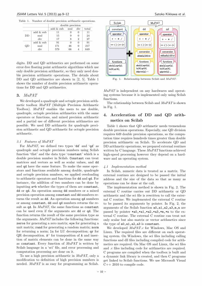
arithmetics at the same time, formulas should be ex-pressed without numerical data types, and change ofdata types should be done dynamically. For these pur-pose, Scilab [3], a free and open source numerical soft-ware, was chosen to implement MuPAT. MuPAT worksindependently on any hardwares and operating systemssince MuPAT is using pure Scilab functions. An inter-preted language Scilab incurs a big overhead, but it ispossible to accelerate its operations by using externalroutines written in C or Fortran.We use DD [4] arithmetic for quadruple precision
arithmetic and QD [5] arithmetic for octuple precisionarithmetic. QD arithmetic needs tens or hundreds ofdouble precision operations for an octuple precision op-eration, then it consumes hundreds or thousands of timecompared to the double precision operation. To accel-erate QD and DD operations, we have implementedMuPAT c using external C routines on Scilab. Mu-PAT c can also accelerate matrix or vector operations
frequently used in numerical analysis. The computationspeed of MuPAT c is 90–1200 times faster than that ofMuPAT.To confirm the effectiveness of MuPAT c and Mu-
PAT, we applied double, quadruple and octuple preci-sion arithmetics to eigenvalue computation. The Lanczosmethod is often used for tridiagonalization but is knownto lose orthogonality because of roundoff error. We com-pared 9 combinations of three different precision arith-metics for tridiagonalization by the Lanczos method andeigenvalue computation by shifted QRmethod. We couldget accurate eigenvalues only when we used octuple pre-cision arithmetic for tridiagonalization, so it becomesclear that high precision arithmetic is essential for theLanczos method.
2. Features of DD and QD arithmetics
DD (Double-Double) is the way to represent a quadru-ple precision number with two double precision numbersand QD (Quad-Double) is the way to represent an oc-tuple precision number with four double precision num-bers.QD number A is represented as stated below with
a0, a1, a2, a3 where a0, a1, a2, a3 are double precisionnumbers.
A = a0 + a1 + a2 + a3,
with
|ai+1| ≤1
2ulp(ai), i = 0, 1, 2,
where ulp stands for ‘unit in the last place’. A DD num-ber is 31 decimal digits and a QD number is 63 decimal
– 9 –
JSIAM Letters Vol. 5 (2013) pp.9–12 Satoko Kikkawa et al.
Table 1. Number of double precision arithmetic operations.
double precision
add & sub mul div total
add & sub 11 0 0 11DD mul 15 9 0 24
div 17 8 2 27
add & sub 91 0 0 91QD mul 171 46 0 217
div 579 66 4 649
digits. DD and QD arithmetics are performed on someerror-free floating point arithmetic algorithms which useonly double precision arithmetic, so they only need dou-ble precision arithmetic operations. The details aboutDD and QD arithmetics are shown in [2, 5]. Table 1shows the number of double precision arithmetic opera-tions for DD and QD arithmetics.
3. MuPAT
We developed a quadruple and octuple precision arith-metic toolbox MuPAT (Multiple Precision ArithmeticToolbox). MuPAT enables the users to use double,quadruple, octuple precision arithmetics with the sameoperators or functions, and mixed precision arithmeticand a partial use of different precision arithmetics arepossible. We used DD arithmetic for quadruple preci-sion arithmetic and QD arithmetic for octuple precisionarithmetic.
3.1 Features of MuPAT
For MuPAT, we defined two types ‘dd’ and ‘qd’ asquadruple and octuple precision numbers using Scilabfunction ‘tlist’ and the data type ‘constant’ which is adouble precision number in Scilab. Constant can treatmatrices and vectors as well as scalar values, and dd
and qd have the same feature. To make the same oper-ators and functions available among double, quadrupleand octuple precision numbers, we applied overloadingto arithmetic operators and functions for dd and qd. Forinstance, the addition of two numbers can be done byinputting a+b whether the types of them are constant,dd or qd. An operation among dd numbers or a mixedprecision operation among constant and dd numbers re-turns the result as dd. An operation among qd numbersor among constant, dd and qd numbers returns the re-sult as qd. In MuPAT, the same functions as constantcan be used even if the arguments are dd or qd. Thefunction returns the result of the same precision type asthe arguments. MuPAT includes the following functions:zeros for generating a zero matrix; eye for generating aunit matrix; rand for generating a random matrix; normfor returning a norm; lu for LU decomposition; qr forQR decomposition. A’ for transposition of A and inser-tion of matrix elements can be done in the same wayas constant. Every function of MuPAT is written byScilab language in a ‘sci’ file, and error processing andcomputation processing are done on it.To use a high precision arithmetic in MuPAT, only a
modification to definition of high precision numbers isneeded. MuPAT is as easy for programming as Scilab.
Fig. 1. Relationship between Scilab and MuPAT.
MuPAT is independent on any hardwares and operat-ing systems because it is implemented only using Scilabfunctions.The relationship between Scilab and MuPAT is shown
in Fig. 1.
4. Acceleration of DD and QD arith-
metics on Scilab
Table 1 shows that QD arithmetic needs tremendousdouble precision operations. Especially, one QD divisionrequires 649 double precision operations, so the compu-tation time requires hundreds times greater than doubleprecision arithmetic on Scilab. To accelerate QD andDD arithmetic operations, we prepared external routineswritten by C language. TheseMuPAT functions achievedhigh-speed processing however they depend on a hard-ware and an operating system.
4.1 Implementation method
In Scilab, numeric data is treated as a matrix. Theexternal routines are designed to be passed the initialaddress and the size of the data so that as many asoperations can be done at the call.The implementation method is shown in Fig. 2. The
external C routine carries out DD arithmetic or QDarithmetic and the sci file is rewritten to call the exter-nal C routine. We implemented the external C routineto be passed its arguments by pointer. In Fig. 2, thearguments of the Scilab function a0,a1,a2,a3,m,n arepassed by pointer *a0,*a1,*a2,*a3,*m,*n to the ex-ternal C routine. The external C routine can treat notonly scalar but also matrix or vector arithmetics sincethe type of a0,a1,a2,a3 is constant.We developed MuPAT c for Windows, Mac OS and
Linux. The required files are different on each operat-ing system. On Windows, the sci files including callingfunctions and dll files including compiled code for arith-metics are required. On Mac OS and Linux, the sci filesand .c files including code for arithmetics are required.C programs are compiled when the toolbox is built anda dynamic link library is created, and then C programsget linked to Scilab functions. We use Microsoft VisualC++ 2010 to compile code.
– 10 –

JSIAM Letters Vol. 5 (2013) pp.9–12 Satoko Kikkawa et al.
Table 2. Computation time in seconds; the ratio is between parentheses.
(i) (ii) (iii) (iv)
x± y xy x / y x+ y x′y Ax
D 0.022 (1) 0.021 (1) 0.017 (1) 0.01 (1) 0.02 (1) 42.03 (1)
DDMuPAT 0.22 (10.4) 0.41 (19.7) 0.43 (25.6) 0.66 (66.0) 197.18 (9859.0) 1182.48 (28.1)
MuPAT c 0.27 (12.1) 0.29 (13.7) 0.31 (18.2) 0.69 (69.0) 1.05 (52.5) 778.91 (18.5)
QDMuPAT 5.31 (241.5) 6.99 (333.0) 39.39 (2317.6) 7.39 (739.0) 5405.47 (270273.5) 11716.7 (278.8)MuPAT c 0.32 (14.7) 0.41 (19.5) 0.42 (24.5) 2.36 (236.0) 4.46 (223.0) 4439.42 (105.6)
sci C
call
function c = %qd_a_qd int qd_a_qd(arguments)
endfunction
arguments
component of A (constant)
size of A (constant)
arguments
call(arguments);
component of A (double)
size of A (int)
Fig. 2. Argument types of each routine.
4.2 Computation time of MuPAT and MuPAT c
Table 2 shows the computation time of MuPAT andMuPAT c in seconds and the ratio of time required forDD and QD arithmetic to time required for double pre-cision arithmetic on Scilab. All experiments are carriedout on Intel Core i5 2.5GHz, 4GB memory and Scilabversion 5.3.3 running on Windows 7. We executed (i) to(iv) repeatedly 104 times. Each result is the average overthree trials.
(i) Scalar addition, subtraction,multiplication, and division(ii) Vector addition (iii) Inner product whose dimension is equal to 103
(iv)Matrix-vector product
In the case of QD basic arithmetics, the computationtime in MuPAT is 241–2317 times greater than that fordouble precision arithmetic, and that in MuPAT c is 14–24 times greater than that for double precision arith-metic. The computation time for QD division is 2317times greater than that for double precision arithmeticand it becomes 24 times in MuPAT c.Using MuPAT c, the computation time of inner prod-
uct is improved from 9859 times to 52 times greater thanthat for double precision arithmetic for DD, and from270273 times to 223 times for QD. The computationtime of Matrix-vector product for DD is 28 times andthat for QD is 278 times greater than that for doubleeven in MuPAT.MuPAT c can run 90–1200 times faster than MuPAT.
MuPAT c is implemented to reduce the computationtime efficiently when more operations are executed atone call. Therefore, QD division and inner product cansignificantly reduce the computation time since theyneed tremendous double precision operations.To confirm a calling overhead, we compared (a) and
(b) for DD and QD arithmetics.
(a) Scalar addition : (x+ y) repeats 106 times
Table 3. 9 combinations of three different precisions.
Eigenvalue computationdouble quadruple octuple
Tridiagonalizationdouble D D D Q D O
quadruple Q D Q Q Q O
octuple O D O Q O O
(b) Vector addition : x+y whose dimension is equal to106
In the case of DD, it took 25.9 seconds for (a) and0.10 seconds for (b), then a calling overhead is about2.6× 10−5 seconds. In the case of QD, it took 32.5 sec-onds for (a) and 0.31 seconds for (b), then a calling over-head is about 3.6 × 10⁻⁵ seconds. The users should beencouraged to use matrix or vector operations ratherthan use scalar operations to avoid calling overheads.
5. Arithmetic precision for tridiagonal-
ization by the Lanczos method
To verify the effectiveness of fast high precision arith-metics, we applied DD and QD arithmetics to eigenvaluecomputation for a real symmetric n× n matrix A.To compute the eigenvalues of a real symmetric ma-
trix A, the matrix A is tridiagonalized to an equivalenttridiagonal matrix, then the eigenvalues of the tridiago-nal matrix are computed. The Lanczos method can con-struct an equivalent tridiagonal matrix as generating or-thogonal bases one after another. The Lanczos methodis useful for a large sparse matrix since it is not neces-sary to modify the matrix A, but roundoff error causesthe Lanczos vectors to lose orthogonality [6].In this section, we analyzed arithmetic precision for
tridiagonalization by the Lanczos method and eigenvaluecomputation by shifted QR method for the tridiagonalmatrix. Table 3 shows 9 combinations of using double,quadruple and octuple precision arithmetics for each ofthe tridiagonalization and the eigenvalue computationwhere D, Q and O stand for double, quadruple and octu-ple precision arithmetics respectively. We assumed thatthe true solution is equal to the computation result pro-duced by the function ‘Eigenvalues’ of Mathematica.We tested ‘bcsstk02’ and ‘nos4’ from MatrixMarket
(http://math.nist.gov/MatrixMarket/) with the initial
vector v = (0, 1, 0, . . . , 0)Tfor the Lanczos method. For
bcsstk02, the dimension is 66, the number of nonzeroentries is 2211, and the condition number is 4.3×10³. Fornos4, they are 100, 347, 1.6× 10³ respectively. Matriceshave no multiple eigenvalues.
– 11 –

JSIAM Letters Vol. 5 (2013) pp.9–12 Satoko Kikkawa et al.
Fig. 3. Comparison of computed λ and true λ for bcsstk02.
Fig. 4. Comparison of computed λ and true λ for nos4.
5.1 Comparison of arithmetic precision
First, we computed
max1≤i≤n
|λi − λ†i | († = O D,O Q,O O)
where λO D, λO Q, λO O and λ represent the eigenvaluesof O D,O Q,O O and the true solution respectively. Theerror of each result was 9.8 × 10⁻¹¹ for bcsstk02 and2.0 × 10−15 for nos4 at the maximum and there wasnot much difference among λO D, λO Q, and λO O. Therewas not also much difference among λD D, λD Q, λD O oramong λQ D, λQ Q, λQ O. This means that using a highprecision arithmetic for eigenvalue computation does notaffect to the final results.Next, we fixed the arithmetic precision to D for eigen-
value computation and compared O D,Q D,D D chang-ing the precision for tridiagonalization by the Lanczosmethod. Figs. 3 and 4 illustrate the difference betweenλ and λ. (λ, λ) are plotted where λ is the result of eachO D,Q D,D D. The closer the point is to the dottedline λ = λ, the more accurate λ is. For bcsstk02 andnos4, the absolute error of λO D was 9.8 × 10⁻¹¹ and1.0×10−15 at the maximum, so every eigenvalue of O Dwas nearly equal to λ. Using D D or Q D, some multipleeigenvalues appeared.Accurate eigenvalues were obtained by using octuple
precision arithmetic for tridiagonalization by the Lanc-zos method however they could not be obtained by usingdouble or quadruple precision arithmetic. It is impor-tant to use higher precision, especially octuple precisionarithmetic for tridiagonalization by the Lanczos methodin cases of bcsstk02 and nos4. On the other hand, double
precision arithmetic is enough for computing eigenvaluesof a tridiagonal matrix since a high precision arithmetichad no effect to the results. Comparison of the Lanc-zos method with reorthogonalization in double precisionand simple the Lanczos process in higher precision is ourfuture work.
6. Conclusion
We have developed a Multiple Precision ArithmeticToolbox MuPAT on Scilab. In MuPAT, quadruple andoctuple precision arithmetics can be treated as well asdouble precision arithmetic.MuPAT c is a high-speed version using external rou-
tines written by C language. To reduce overheads, exter-nal C routines are implemented to be passed matrix orvector values by pointer so that one call can carry outas many operations as possible. MuPAT c reduces thecomputation time for QD arithmetics from 241–270273times to 14–236 times greater than that for double preci-sion arithmetic, and the computation time for DD arith-metics from 10–9859 times to 12–69 times.We analyzed arithmetic precision for tridiagonaliza-
tion using MuPAT c. We compared 9 combinations ofusing double, quadruple, and octuple precision arith-metics for tridiagonalization by the Lanczos method andeigenvalue computation by shifted QRmethod. Accurateeigenvalues were obtained only by using octuple preci-sion arithmetic for tridiagonalization. It becomes clearthat a higher precision arithmetic is essential for tridi-agonalization by the Lanczos method.To use MuPAT and MuPAT c, only a modification to
definition of high precision numbers is required. MuPATand MuPAT c are efficient toolboxes for mixed precisionarithmetic, thus they should be important for numericalanalysis.
References
[1] MuPAT and QuPAT, http://www.mi.kagu.tus.ac.jp/qupa
t.html.[2] T. Saito, E. Ishiwata and H. Hasegawa, Development of
quadruple precision arithmetic toolbox QuPAT on Scilab, in:Proc. of ICCSA 2010, Part II, D. Taniar et al. eds., LNCS,
Vol. 6017, pp. 60–70, Springer-Verlag, Berlin, 2010.[3] Scilab, http://www.scilab.org/.[4] T. J. Dekker, A floating-point technique for extending the
available precision, Numer. Math., 18 (1971), 224–242.
[5] Y.Hida, X. S.Li and D.H.Bailey, Quad-double arithmetic: al-gorithms, implementation, and application, Technical ReportLBNL-46996, 2000.
[6] J. W. Demmel, Applied Numerical Linear Algebra, SIAM,Philadelphia, 1997.
– 12 –

JSIAM Letters Vol.5 (2013) pp.13–16 c⃝2013 Japan Society for Industrial and Applied Mathematics J S I A MLetters
Remarks on the rate of strong convergence of
Euler-Maruyama approximation for SDEs driven by
rotation invariant stable processes
Hiroya Hashimoto1 and Takahiro Tsuchiya2
1 Ritsumeikan University, 1-1-1 Noji-higashi, Kusatsu, Shiga 525-8577, Japan2 The University of Aizu, Tsuruga, Ikki-machi, Aizu-Wakamatsu City, Fukushima 965-0826,Japan
E-mail hiroya hashimoto nifty.com
Received October 31, 2012, Accepted November 6, 2012
Abstract
In this paper, we consider Euler-Maruyama approximations for 1-dimensional stochastic dif-ferential equations (SDEs) driven by rotation invariant (i.e. symmetric) α stable processesand discuss their rate of strong convergence by numerical simulations. We also study the re-lationship between the convergence rate and the index α of rotation invariant stable processand/or the exponent γ of the Holder continuity of the diffusion coefficient.
Keywords Euler-Maruyama approximation, rotation invariant stable processes, stochasticdifferential equations
Research Activity Group Mathematical Finance
1. Introduction
In mathematical finance, the arbitrage-free price of anoption whose pay-off is g(XT ), where X is the price pro-cess of the underlying asset, g is typically a continuousbut not smooth function, and T is the maturity, is givenby its expectation with respect to an equivalent martin-gale measure. The price process of the underlying is oftengiven as the solution to a stochastic differential equation(SDE). The distribution of XT , which is required to cal-culate the expectation in one dimensional integration,is generally unavailable. Instead, one needs to resort tosome numerical procedures involving approximation ofSDE and Monte Carlo simulation of the driving pro-cess. The weak rate of convergence of an approximationscheme of the SDE is thus quite important to estimatethe error. The rate of strong convergence is, on the otherhand, related to the hedging error rather than the priceitself. Suppose that the pay-off g(XN
T ) is properly hedged(in theory) with an initial cost which is not necessarilythe fair price. Then assuming that g(XT ) is the reality,the hedging error is evaluated by, for example,
E[∥∥g(XT )− g(XN
T )∥∥]
for some norm ∥ · ∥. In any case it is dominated by
E
[supt
∣∣Xt −XNt
∣∣p] (1)
for some p. In view of this application, we discuss therate of strong convergence of SDEs, i.e., the convergencewith respect to the norm appearing in (1).The both rates of weak and strong convergence are
well-understood in the cases of Wiener process drivenSDEs. In mathematical finance, however, the use of Levydriven SDE has become popular. So, in this paper, we
concentrate on the Levy driven cases. In the context ofthe rate of weak convergence, some results of the con-vergence rate are given by Protter and Talay [1]. On theother hand, the rate of strong convergence is not knownas far as the authors know. We are particularly interestedin the rates of strong convergence of Euler-Maruyamaapproximation for a jump type SDEs. In this paper, asthe first step, we focus on the convergent rate of theexponential rotation invariant α stable process since thecoefficient is regular and the class has interesting proper-ties. (The case of α = 2 is corresponding with Brownianmotion and the other has pure jump if α < 2.)In Section 2, we introduce the method and the theo-
retical background. In Section 3, we give numerical sim-ulations, where the error of strong approximation is con-jectured.
2. Method
Let us recall the definition of the rotation invari-ant α stable process. (In the 1-dimensional case, ro-tation invariance is tantamount to symmetry.) Let(Ω,F , Ft,P) be a filtered probability space with usualconditions.
Definition 1 Z = Z(t); t ≥ 0 is an Ft-rotation in-variant α stable process if Z(0) = 0, it is cadlag (rightcontinuous with left limits), Ft-adapted and
E[exp(iξ(Z(t)− Z(s)))|Fs]
= exp(−(t− s)|ξ|α) a.s. for any s < t, ξ ∈ R.
We consider 1-dimensional SDE with respect to therotation invariant α stable process (1 < α < 2) in the
– 13 –
JSIAM Letters Vol. 5 (2013) pp.13–16 Hiroya Hashimoto et al.
following form
X(t) = X(0) +
∫ t
0
σ(X(s−))dZ(s), t ∈ [0, T ]. (2)
Let ∆ : 0 = t0 < t1 < · · · < tk < tk+1 < · · · < tn = Tbe a partition of [0, T ]. We construct Euler-Maruyamaapproximation of the solution of (2):
X∆(0) := X(0),
X∆(t) := X∆(tk) + σ(X∆(tk−))(Z(t)− Z(tk)),
for tk ≤ t < tk+1.
As to the strong convergence of the approximationscheme, the following is established in [2].
Theorem 2 ([2]) Assuming the following conditionsfor the coefficient of (2);
• σ(x) is uniformly continuous on R,• there exists a non-negative increasing function ρ de-fined on [0,∞) such that: ρ(0) = 0,
∫0+ρ−1(x)dx =
∞, |σ(x)− σ(y)|α ≤ ρ(|x− y|), for any x, y ∈ R,the Euler-Maruyama approximation X∆(t) satisfies
lim∥∆∥→0
E
[sup
0≤t≤T|X∆(t)−X(t)|β
]= 0,
for any β ∈ (1, α),
where X(t) is a unique solution of (2) with bounded ini-tial value X(0).
To simulate the approximation scheme, we follow themethod of computer simulation of rotation invariant (i.e.symmetric) α stable random variable Z ∼ Sα(1, 0, 0)with α = 2 by Janicki and Weron [3] (see [3] for furtherinformation);
• generate a random variable V uniformly distributedon (−π/2, π/2) and an exponential random variableW with mean 1;
• compute
Z =sin(αV )
(cos(V ))1α
×(cos(V − αV )
W
) 1−αα
.
2.1 Linear SDE
Now, we consider the numerical simulation for the so-lutions of following SDE;
X(t) = 1 +
∫ t
0
X(s−)dZ(s). (3)
The solution of (3) is given by Dolean-Dade [4] as fol-lows;
X(t) = exp(Z(t))
[∏s≤t
(1 + ∆Z(s)) exp(−∆Z(s))
], (4)
where ∆Z(s) = Z(s)− Z(s−).Let us fix a positive integer I ∈ N and partition the
interval [0, T ] into I equal subintervals;
ti = iτ, for i = 0, 1, 2, . . . , I, where τ = T/I.
We approximate the explicit solution (4) by a discretetime process Xτ (ti)Ii=0 defined by
Xτ (ti) = exp(Zτ (ti))
×
[ ∏tk≤ti
(1 + ∆Zτ (tk)) exp(−∆Zτ (tk))
],
where we approximate the rotation invariant α stableprocess Z(t) : t ∈ [0, T ] by a discrete time processZτ (ti)Ii=0 defined by
1. Zτ (t0) = 0;
2. for i = 1, 2, . . . , I,
Zτ (ti) =i∑
k=1
∆Zτ (tk), ∆Zτ (tk) =(TI
) 1α × Zk,
where Zk ∼ Sα(1, 0, 0) are i.i.d. random variables.
For another integer IEM ≪ I, we construct Euler-Maruyama approximations of the solution of (3)with stepsize T/IEM by a discrete time processX∆(ti)Ii=0 = X∆(IEM )(ti)Ii=0 defined by X∆(t0) = 1and
X∆(ti) = X∆
(kTIEM
)+X∆
(kTIEM
)(Zτ (ti)− Zτ
(kTIEM
)),
for kTIEM
≤ ti < (k+1)TIEM
.
It is noteworthy that for the SDE (3), when IEM = I,Xτ (ti)Ii=0 = X∆(ti)Ii=0. We shall show this byinduction. Obviously, Xτ (t0) = X∆(t0). We assumeXτ (tk) = X∆(tk) for k ∈ N. Then
X∆(tk+1) = X∆(tk) +X∆(tk)×∆Zτ (tk+1)
= X∆(tk)× (1 + ∆Zτ (tk+1))
= exp(Zτ (tk))
×
[ ∏tl≤tk
(1 + ∆Zτ (tl)) exp(−∆Zτ (tl))
]
× (1 + ∆Zτ (tk+1))
= exp(Zτ (tk))× exp(∆Zτ (tk+1))
×
[ ∏tl≤tk+1
(1 + ∆Zτ (tl)) exp(−∆Zτ (tl))
]
= Xτ (tk+1).
Therefore, we obtain Xτ (ti) = X∆(ti) for i =0, 1, 2, . . . , I.Let us define the approximation error ε1(α, β, IEM ) as
follows;
ε1(α, β, IEM ) := maxti|X∆(ti)−Xτ (ti)|β .
Here we consider the case with IEM ≪ I. This meansthat we regard Xτ as a proxy of the true value X.We also consider the case with α = 2, namely we con-
sider SDEs driven by Brownian motion as a benchmark.We approximate Brownian motion B(t) : t ∈ [0, T ] bya discrete time process Bτ (ti)Ii=0 given by
1. Bτ (t0) = 0;
– 14 –
JSIAM Letters Vol. 5 (2013) pp.13–16 Hiroya Hashimoto et al.
2. for i = 1, 2, . . . , I
Bτ (ti) =i∑
k=1
∆Bτ (tk), ∆Bτ (tk) =(TI
) 12 ×Bk,
where Bk ∼ N(0, 1) are i.i.d. random variables.
As is well-known, the linear SDE;
V (t) = 1 +
∫ t
0
V (s)dB(s), (5)
has the explicit solution
V (t) = exp(B(t)− t
2
). (6)
We approximate the explicit solution (6) by a discretetime process V τ (ti)Ii=0 defined by
V τ (ti) = exp(Bτ (ti)− ti
2
).
Also, we construct Euler-Maruyama approximation ofthe solution of (5) with stepsize T/IEM by a discretetime process V∆(ti)IEM
i=0 defined by V∆(t0) = 1 and
V∆(ti) = V∆
(kTIEM
)+ V∆
(kTIEM
)(Bτ (ti)−Bτ
(kTIEM
)),
for kTIEM
≤ ti < (k+1)TIEM
.
We then define the approximation error ε1(2.0, β, IEM )for IEM ≪ I as
ε1(2.0, β, IEM ) := maxti|V∆(ti)− V τ (ti)|β ,
which is slightly different in spirit from the ones withα = 2 in that the value V τ (ti) is precise though it stillis a proxy for the stochastic process V (t)t≥0.
2.2 SDE with non-Lipschitz coefficient
We also consider the numerical simulation for the so-lutions of following SDE;
Y (t) = 1 +
∫ t
0
|Y (s−)|γdZ(s), (7)
where γ ∈ [1/α, 1). The SDE (7) cannot be solved explic-itly. However, we regard the approximation with smallenough stepsize as benchmark, as we did above.For fixed integer IEM , we construct Euler-Maruyama
approximation of the solution of (7) with stepsizeT/IEM by a discrete time process Y∆(ti)Ii=0 =Y∆(IEM )(ti)Ii=0 defined by Y∆(t0) = 1 and
Y∆(ti) = Y∆
(kTIEM
)+∣∣∣Y∆( kT
IEM
)∣∣∣γ(Zτ (ti)− Zτ( kTIEM
)),
for kTIEM
≤ ti < (k+1)TIEM
.
We define the approximation error ε2(α, β, γ, IEM ) asbefore;
ε2(α, β, γ, IEM ) := maxti|Y∆(ti)− Y∆(I)(ti)|β .
3. Numerical experiments
In this section, let us present numerical examples. Wehave used SAS on Windows 7 over a personal computerhaving Intel CPU Core i5-2400 3.1GHz. In all cases wehave chosen T = 1 and I = 214.
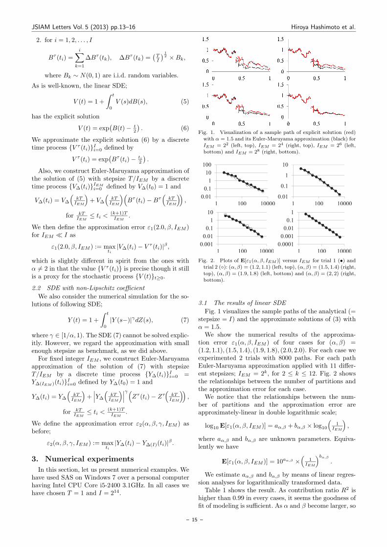
Fig. 1. Visualization of a sample path of explicit solution (red)with α = 1.5 and its Euler-Maruyama approximation (black) for
IEM = 22 (left, top), IEM = 24 (right, top), IEM = 26 (left,bottom) and IEM = 28 (right, bottom).
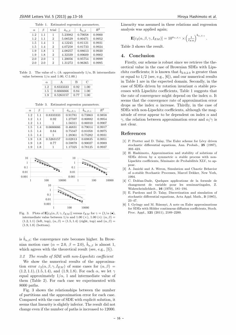
Fig. 2. Plots of E[ε1(α, β, IEM )] versus IEM for trial 1 (•) andtrial 2 (): (α, β) = (1.2, 1.1) (left, top), (α, β) = (1.5, 1.4) (right,top), (α, β) = (1.9, 1.8) (left, bottom) and (α, β) = (2, 2) (right,
bottom).
3.1 The results of linear SDE
Fig. 1 visualizes the sample paths of the analytical (=stepsize = I) and the approximate solutions of (3) withα = 1.5.We show the numerical results of the approxima-
tion error ε1(α, β, IEM ) of four cases for (α, β) =(1.2, 1.1), (1.5, 1.4), (1.9, 1.8), (2.0, 2.0). For each case weexperimented 2 trials with 8000 paths. For each pathEuler-Maruyama approximation applied with 11 differ-ent stepsizes; IEM = 2k, for 2 ≤ k ≤ 12. Fig. 2 showsthe relationships between the number of partitions andthe approximation error for each case.We notice that the relationships between the num-
ber of partitions and the approximation error areapproximately-linear in double logarithmic scale;
log10 E[ε1(α, β, IEM )] = aα,β + bα,β × log10
(1
IEM
),
where aα,β and bα,β are unknown parameters. Equiva-lently we have
E[ε1(α, β, IEM )] = 10aα,β ×(
1IEM
)bα,β
.
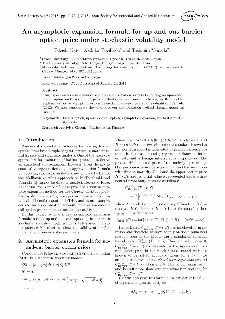
We estimate aα,β and bα,β by means of linear regres-sion analyses for logarithmically transformed data.Table 1 shows the result. As contribution ratio R2 is
higher than 0.99 in every cases, it seems the goodness offit of modeling is sufficient. As α and β become larger, so
– 15 –
JSIAM Letters Vol. 5 (2013) pp.13–16 Hiroya Hashimoto et al.
Table 1. Estimated regression parameters.
α β trial aα,β bα,β R2
1.2 1.1 1 5.23982 0.79058 0.9900
1.2 1.1 2 5.08529 0.80471 0.9952
1.5 1.4 1 4.12245 0.81121 0.99311.5 1.4 2 4.07258 0.81733 0.9924
1.9 1.8 1 4.08257 0.88613 0.99201.9 1.8 2 4.32339 0.89609 0.9902
2.0 2.0 1 1.20056 0.95754 0.99992.0 2.0 2 1.31272 0.96365 0.9995
Table 2. The value of γ. (A: approximately 1/α, B: intermediatevalue between 1/α and 1.00, C:1.00.)
α A B C
1.2 0.8333333 0.92 1.00
1.5 0.6666666 0.84 1.00
1.9 0.5263157 0.77 1.00
Table 3. Estimated regression parameters.
α β γ aα,β,γ bα,β,γ R2
1.2 1.1 0.8333333 0.91781 0.73863 0.9858
1.2 1.1 0.92 1.27597 0.80882 0.99541.2 1.1 1 1.56311 0.86910 0.9907
1.5 1.4 0.6666666 0.46831 0.79014 0.99171.5 1.4 0.84 0.75347 0.81058 0.9975
1.5 1.4 1 1.28361 0.75282 0.9931
1.9 1.8 0.5263157 0.02813 0.69835 0.99511.9 1.8 0.77 0.59878 0.90027 0.99891.9 1.8 1 1.17325 0.78125 0.9937
Fig. 3. Plots of E[ε2(α, β, γ, IEM )] versus IEM for γ = 1/α (•),intermediate value between 1/α and 1.00 (×), 1.00 (): (α, β) =(1.2, 1.1) (left, top), (α, β) = (1.5, 1.4) (right, top) and (α, β) =(1.9, 1.8) (bottom).
is bα,β ; the convergence rate becomes higher. In Brow-
nian motion case (α = 2.0, β = 2.0), bα,β is almost 1,which agrees with the theoretical result (see, e.g., [5]).
3.2 The results of SDE with non-Lipschitz coefficient
We show the numerical results of the approxima-tion error ε2(α, β, γ, IEM ) of some cases for (α, β) =(1.2, 1.1), (1.5, 1.4), and (1.9, 1.8). For each α, we let γequal approximately 1/α, 1 and intermediate value ofthem (Table 2). For each case we experimented with8000 paths.Fig. 3 shows the relationships between the number
of partitions and the approximation error for each case.Compared with the case of SDE with explicit solution, itseems that linearity is slightly inferior. The result did notchange even if the number of paths is increased to 12000.
Linearity was assumed in these relations and regressionanalysis was applied again;
E[ε2(α, β, γ, IEM )] = 10aα,β,γ ×(
1IEM
)bα,β,γ
.
Table 3 shows the result.
4. Conclusion
Firstly, our scheme is robust since we retrieve the the-oretical value in the case of Brownian SDEs with Lips-chitz coefficients; it is known that b2.0,2.0 is greater thanor equal to 1/2 (see, e.g., [6]), and our numerical resultsin Table 1 are in the expected domain. Secondly, in thecase of SDEs driven by rotation invariant α stable pro-cesses with Lipschitz coefficients, Table 1 suggests thatthe rate of convergence might depend on the index α. Itseems that the convergence rate of approximation errordrops as the index α increase. Thirdly, in the case ofSDEs with non-Lipschitz coefficients, although the mag-nitude of error appear to be dependent on index α andγ, the relation between approximation error and α/γ isnot clear.
References
[1] P. Protter and D. Talay, The Euler scheme for Levy drivenstochastic differential equations, Ann. Probab., 25 (1997),
393–423.[2] H. Hashimoto, Approximation and stability of solutions of
SDEs driven by a symmetric α stable process with non-
Lipschitz coefficients, Seminaire de Probabilites XLV, to ap-pear.
[3] A. Janicki and A. Weron, Simulation and Chaotic Behaviorof α-stable Stochastic Processes, Marcel Dekker, New York,
1994.[4] C. Dolean-Dade, Quelques applications de la formule de
changement de variable pour les semimartingales, Z.Wahrscheinlichkeit., 16 (1970), 181–194.
[5] E. Pardoux and D. Talay, Discretization and simulation ofstochastic differential equations, Acta Appl. Math., 3 (1985),23–47.
[6] I. Gyongy and M. Rasonyi, A note on Euler approximations
for SDEs with Holder continuous diffusion coefficients, Stoch.Proc. Appl., 121 (2011), 2189–2200.
– 16 –
JSIAM Letters Vol.5 (2013) pp.17–20 c⃝2013 Japan Society for Industrial and Applied Mathematics J S I A MLetters
An asymptotic expansion formula for up-and-out barrier
option price under stochastic volatility model
Takashi Kato1, Akihiko Takahashi2 and Toshihiro Yamada2,3
1 Osaka University, 1-3, Machikaneyama-cho, Toyonaka, Osaka 560-8531, Japan2 The University of Tokyo, 7-3-1 Hongo, Bunkyo, Tokyo 113-0033 Japan3 Mitsubishi UFJ Trust Investment Technology Institute Co., Ltd. (MTEC), 2-6, Akasaka 4-Chome, Minato, Tokyo 107-0052 Japan
E-mail kato sigmath.es.osaka-u.ac.jp
Received January 17, 2013, Accepted January 21, 2013
Abstract
This paper derives a new semi closed-form approximation formula for pricing an up-and-outbarrier option under a certain type of stochastic volatility model including SABR model byapplying a rigorous asymptotic expansion method developed by Kato, Takahashi and Yamada(2012). We also demonstrate the validity of our approximation method through numericalexamples.
Keywords barrier option, up-and-out call option, asymptotic expansion, stochastic volatil-ity model
Research Activity Group Mathematical Finance
1. Introduction
Numerical computation schemes for pricing barrieroptions have been a topic of great interest in mathemat-ical finance and stochastic analysis. One of the tractableapproaches for evaluation of barrier options is to derivean analytical approximation. However, from the math-ematical viewpoint, deriving an approximation formulaby applying stochastic analysis is not an easy task sincethe Malliavin calculus approach as in Takahashi andYamada [1] cannot be directly applied. Recently, Kato,Takahashi and Yamada [2] has provided a new asymp-totic expansion method for the Cauchy–Dirichlet prob-lem by developing a rigorous perturbation scheme in apartial differential equation (PDE), and as an example,derived an approximation formula for a down-and-outcall option price under a stochastic volatility model.In this paper, we give a new asymptotic expansion
formula for an up-and-out call option price under astochastic volatility model which is widely used in trad-ing practice. Moreover, we show the validity of our for-mula through numerical experiments.
2. Asymptotic expansion formula for up-
and-out barrier option prices
Consider the following stochastic differential equation(SDE) in a stochastic volatility model:
dSεt = (c− q)Sεt dt+ σεtSεt dB
1t ,
Sε0 = S,
dσεt = ελ(θ − σεt )dt+ ενσεt
(ρdB1
t +√
1− ρ2 dB2t
),
σε0 = σ,
where S, σ, c, q > 0, ε ∈ [0, 1), λ, θ, ν > 0, ρ ∈ [−1, 1] andB = (B1, B2) is a two dimensional standard Brownianmotion. This model is motivated by pricing currency op-tions. In this case, c and q represent a domestic inter-est rate and a foreign interest rate, respectively. Theprocess Sε denotes a price of the underlying currency.Our purpose is to evaluate an up-and-out barrier optionwith time-to-maturity T − t and the upper barrier priceH(> S), and its initial value is represented under a risk-neutral probability measure as follows:
CSV,εBarrier(T − t, S)
= E[e−c(T−t)f(SεT−t)1τ(0,H)(Sε)>T−t
],
where f stands for a call option payoff function f(s) =maxs−K, 0 for some K > 0. Here, the stopping timeτ(0,H)(S
ε) is defined as
τ(0,H)(Sε) = inft ∈ [0, T ];Sεt /∈ (0,H) (inf ∅ :=∞).
Remark that CSV,εBarrier(T − t, S) has no closed-form so-lution and therefore we have to rely on some numericalmethod such as the Monte–Carlo simulation in orderto calculate CSV,εBarrier(T − t, S). However, when ε = 0,
CSV,0Barrier(T − t, S) corresponds to the up-and-out bar-rier option price in the Black-Scholes model which isknown to be solved explicitly. Then, for ε > 0, weare able to derive a semi closed-form expansion aroundCSV,0Barrier(T − t, S) when ε ↓ 0. This is our main resultand hereafter we show our approximation method forCSV,εBarrier(T − t, S).Clearly, applying Ito’s formula, we can derive the SDE
of logarithmic process of Sεt as
dXεt =
[c− q − 1
2(σεt )
2
]dt+ σεt dB
1t ,
– 17 –

JSIAM Letters Vol. 5 (2013) pp.17–20 Takashi Kato et al.
Xε0 = x := logS.
Then we can rewrite CSV,εBarrier(T − t, S) as
CSV,εBarrier(T − t, ex)
= E[e−c(T−t)f(Xε
T−t)1τD(Xε)>T−t
],
where f(x) = maxex − K, 0 and D = (−∞, logH).Note that
τD(Xε) = inft ∈ [0, T ];Xε
t /∈ D = τ(0,H)(Sε).
Let uε(t, x) = CSV,εBarrier(T − t, ex) for t ∈ [0, T ] andx ∈ R. Then uε(t, x) satisfies the following PDE:
(∂∂t + L ε − c
)uε(t, x) = 0, (t, x) ∈ (0, T ]×D,
uε(T, x) = f(x), x ∈ D,uε(t, logH) = 0, t ∈ [0, T ],
where
L ε =
(c− q − 1
2σ2
)∂
∂x+
1
2σ2 ∂
2
∂x2
+ ερνσ2 ∂2
∂x∂σ+ ελ(θ − σ) ∂
∂σ+ ε2
1
2ν2σ2 ∂
2
∂σ2.
As mentioned above, when ε = 0, we can obtainthe explicit value of u0(t, x). In this case, u0(t, x) =CBSBarrier(T − t, ex, σ,H) represents the price of the up-and-out barrier call option under the Black–Scholesmodel. We have
CBSBarrier = CBSVanilla − C,
where
CBSVanilla = exe−qTN(d1)−Ke−cTN(d2),
C = exe−qTN(x1)−Ke−cTN(x2)
− exe−qT(H
ex
)2λ
[N(−y)−N(−y1)]
+Ke−cT(H
ex
)2λ−2
×[N(−y + σ
√T)−N
(−y1 + σ
√T)]
with
x1 =x− logH + (c− q)T + 1
2σ2T
σ√T
,
x2 = x1 − σ√T ,
λ =(c− q)σ2
+1
2,
y =2 logH − x− logK + (c− q)T + 1
2σ2T
σ√T
,
y1 =logH − x+ (c− q)T + 1
2σ2T
σ√T
.
See Hull [3] for the details.We can represent u0(t, x) = PDt f(x) by using a semi-
group (PDt )t defined as
PDs g(x) =
∫ logH
−∞e−cs
(1− e−
2(log H−x)(log H−y)
σ2s
)× 1√
2πσ2se−
[y−x−(c−q− 12σ2)s]
2
2σ2s g(y) dy (1)
for a continuous function g with polynomial growth ratewhich satisfies g(x) = 0 on ∂D.The main result of Kato, Takahashi and Yamada [2]
suggests the following approximation formula (asymp-totic expansion formula).
uε(t, x) = CBSBarrier + εe−c(T−t)
×∫ T−t
0
PDs L 01 P
DT−t−sf(x)ds+O(ε2),
where
L 01 =
∂
∂εL ε|ε=0 = ρσ2 ∂2
∂x∂σ+ λ(θ − σ) ∂
∂σ.
Using (1), the term∫ T−t0
PDs L 01 P
DT−t−sf(x) ds is ex-
pressed as follows:∫ T−t
0
PDs L 01 P
DT−t−sf(x)ds
=
∫ T−t
0
∫ logH
−∞e−cs
(1− e−
2(log H−x)(log H−y)
σ2s
) 1√2πσ2s
× e−[y−x−(c−q− 1
2σ2)s]2
2σ2s L 01 P
DT−t−sf(y) dyds. (2)
We are able to compute the integrand of the righthand side of the above formula (2) as
L 01 P
DT−tf(x)
= ec(T−t)[ρσ2 ∂2
∂x∂σCBSBarrier(T − t, ex, σ)
+λ(θ − σ) ∂∂σ
CBSBarrier(T − t, ex, σ)].
Here, ∂CBSBarrier(T, ex)/∂σ and ∂2CBSBarrier(T, e
x)/∂x∂σare concretely expressed as follows:
∂
∂σCBSBarrier(T, e
x)
= e−qT exn(d1)√T − e−qT exn(x1)
√T
− (H −K)e−cTn(x2)−x1σ
+ exe−qT(H
ex
)2λ
×[(logH − x)−4(c− q)
σ3(N(−y)−N(−y1))
+
(n(y)
y′
σ− n(y1)
y′1σ
)]
−Ke−cT(H
ex
)2λ−2
×[(logH − x)−4(c− q)
σ3(N(−y′)−N(−y′1))
– 18 –
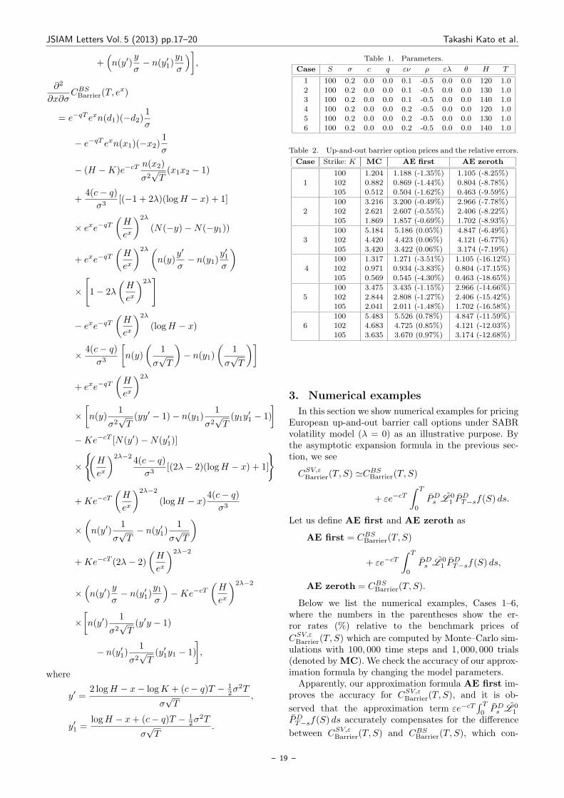
JSIAM Letters Vol. 5 (2013) pp.17–20 Takashi Kato et al.
+(n(y′)
y
σ− n(y′1)
y1σ
)],
∂2
∂x∂σCBSBarrier(T, e
x)
= e−qT exn(d1)(−d2)1
σ
− e−qT exn(x1)(−x2)1
σ
− (H −K)e−cTn(x2)
σ2√T(x1x2 − 1)
+4(c− q)σ3
[(−1 + 2λ)(logH − x) + 1]
× exe−qT(H
ex
)2λ
(N(−y)−N(−y1))
+ exe−qT(H
ex
)2λ(n(y)
y′
σ− n(y1)
y′1σ
)
×
[1− 2λ
(H
ex
)2λ]
− exe−qT(H
ex
)2λ
(logH − x)
× 4(c− q)σ3
[n(y)
(1
σ√T
)− n(y1)
(1
σ√T
)]
+ exe−qT(H
ex
)2λ
×[n(y)
1
σ2√T(yy′ − 1)− n(y1)
1
σ2√T(y1y
′1 − 1)
]−Ke−cT [N(y′)−N(y′1)]
×
(H
ex
)2λ−24(c− q)σ3
[(2λ− 2)(logH − x) + 1]
+Ke−cT(H
ex
)2λ−2
(logH − x)4(c− q)σ3
×(n(y′)
1
σ√T− n(y′1)
1
σ√T
)
+Ke−cT (2λ− 2)
(H
ex
)2λ−2
×(n(y′)
y
σ− n(y′1)
y1σ
)−Ke−cT
(H
ex
)2λ−2
×[n(y′)
1
σ2√T(y′y − 1)
− n(y′1)1
σ2√T(y′1y1 − 1)
],
where
y′ =2 logH − x− logK + (c− q)T − 1
2σ2T
σ√T
,
y′1 =logH − x+ (c− q)T − 1
2σ2T
σ√T
.
Table 1. Parameters.
Case S σ c q εν ρ ελ θ H T
1 100 0.2 0.0 0.0 0.1 -0.5 0.0 0.0 120 1.02 100 0.2 0.0 0.0 0.1 -0.5 0.0 0.0 130 1.03 100 0.2 0.0 0.0 0.1 -0.5 0.0 0.0 140 1.0
4 100 0.2 0.0 0.0 0.2 -0.5 0.0 0.0 120 1.05 100 0.2 0.0 0.0 0.2 -0.5 0.0 0.0 130 1.06 100 0.2 0.0 0.0 0.2 -0.5 0.0 0.0 140 1.0
Table 2. Up-and-out barrier option prices and the relative errors.
Case Strike: K MC AE first AE zeroth
1
100 1.204 1.188 (-1.35%) 1.105 (-8.25%)
102 0.882 0.869 (-1.44%) 0.804 (-8.78%)105 0.512 0.504 (-1.62%) 0.463 (-9.59%)
2100 3.216 3.200 (-0.49%) 2.966 (-7.78%)102 2.621 2.607 (-0.55%) 2.406 (-8.22%)
105 1.869 1.857 (-0.69%) 1.702 (-8.93%)
3100 5.184 5.186 (0.05%) 4.847 (-6.49%)102 4.420 4.423 (0.06%) 4.121 (-6.77%)105 3.420 3.422 (0.06%) 3.174 (-7.19%)
4100 1.317 1.271 (-3.51%) 1.105 (-16.12%)102 0.971 0.934 (-3.83%) 0.804 (-17.15%)105 0.569 0.545 (-4.30%) 0.463 (-18.65%)
5
100 3.475 3.435 (-1.15%) 2.966 (-14.66%)
102 2.844 2.808 (-1.27%) 2.406 (-15.42%)105 2.041 2.011 (-1.48%) 1.702 (-16.58%)
6100 5.483 5.526 (0.78%) 4.847 (-11.59%)102 4.683 4.725 (0.85%) 4.121 (-12.03%)105 3.635 3.670 (0.97%) 3.174 (-12.68%)
3. Numerical examples
In this section we show numerical examples for pricingEuropean up-and-out barrier call options under SABRvolatility model (λ = 0) as an illustrative purpose. Bythe asymptotic expansion formula in the previous sec-tion, we see
CSV,εBarrier(T, S) ≃CBSBarrier(T, S)
+ εe−cT∫ T
0
PDs L 01 P
DT−sf(S) ds.
Let us define AE first and AE zeroth as
AE first = CBSBarrier(T, S)
+ εe−cT∫ T
0
PDs L 01 P
DT−sf(S) ds,
AE zeroth = CBSBarrier(T, S).
Below we list the numerical examples, Cases 1–6,where the numbers in the parentheses show the er-ror rates (%) relative to the benchmark prices of
CSV,εBarrier(T, S) which are computed by Monte–Carlo sim-ulations with 100, 000 time steps and 1, 000, 000 trials(denoted by MC). We check the accuracy of our approx-imation formula by changing the model parameters.Apparently, our approximation formula AE first im-
proves the accuracy for CSV,εBarrier(T, S), and it is ob-
served that the approximation term εe−cT∫ T0PDs L 0
1
PDT−sf(S) ds accurately compensates for the difference
between CSV,εBarrier(T, S) and CBSBarrier(T, S), which con-
– 19 –

JSIAM Letters Vol. 5 (2013) pp.17–20 Takashi Kato et al.
firms the validity of our method. For all cases, we setS = 100, σ = 0.2, c = 0.0, q = 0.0, ρ = −0.5, ελ = 0.0,θ = 0.0 and T = 1.0. In Cases 1, 2 and 3, given εν = 0.1,the upper bound price is set as H = 120, 130, 140, re-spectively, while in Cases 4, 5 and 6, given εν = 0.2,H is set as 120, 130, 140, respectively. Particularly, forthe case of εν = 0.2 (that is, higher volatility of volatil-ity case, Cases 4, 5 and 6), we remark that the errorsof the approximation become slightly larger. However,as observed in comparison between AE first and AEzeroth, we are convinced that the higher order expan-sion improves the approximation further, which will beinvestigated in our next research.
References
[1] A.Takahashi and T.Yamada, An asymptotic expansion with
push-down of Malliavin weights, SIAM J. Financial Math., 3(2012), 95–136.
[2] T. Kato, A. Takahashi and T. Yamada, An asymptotic ex-
pansion for solutions of Cauchy-Dirichlet problem for secondorder parabolic PDEs and its application to pricing barrieroptions, arXiv:1202.3002, 2012.
[3] J.C. Hull, Options, Futures, and Other Derivatives, 6th Edi-
tion, Prentice Hall, New Jersey, 2005.
– 20 –

JSIAM Letters Vol.5 (2013) pp.21–24 c⃝2013 Japan Society for Industrial and Applied Mathematics J S I A MLetters
An application of the Kato-Temple inequality on matrix
eigenvalues to the dqds algorithm for singular values
Takumi Yamashita1, Kinji Kimura1, Masami Takata2 and Yoshimasa Nakamura1
1 Graduate School of Informatics, Kyoto University, Yoshida-Honmachi, Sakyo-ku, Kyoto 606-8501, Japan
2 Academic Group of Information and Computer Sciences, Nara Women’s University, Kita-Uoya-Nishi-machi, Nara 630-8506, Japan
E-mail takumi amp.i.kyoto-u.ac.jp
Received March 8, 2012, Accepted July 6, 2012
Abstract
Choice of suitable shifts strongly influences performance of numerical algorithms with shift forcomputing matrix eigenvalues or singular values. On the dqds (differential quotient differencewith shifts) algorithm for singular values, a new shift strategy is proposed in this paper. Thenew shift strategy includes shifts obtained from an application of the Kato-Temple inequalityon matrix eigenvalues. The dqds algorithm with the new shift strategy is shown to have abetter performance in iteration number than that of the subroutine DLASQ in LAPACK.
Keywords dqds algorithm, shift strategy, implementation
Research Activity Group Algorithms for Matrix / Eigenvalue Problems and their Applications
1. Introduction
Singular value decomposition (SVD) can be adaptedto a wide field of applications. In this paper, we considerthe dqds (differential quotient difference with shifts) al-gorithm [1] as a singular value computation algorithm.Before execution of the dqds algorithm, an input ma-trix is transformed into an upper bidiagonal matrixB(0) by sequential application of the well-known House-holder transforms. The dqds algorithm corresponds tothe Cholesky transform with shift
(B(n+1))⊤B(n+1) = B(n)(B(n))⊤ − s(n)I
for n = 0, 1, 2, . . . , where s(n) and I are shift (non-negative) and the unit matrix, respectively. It is knownthat the square of a lower bound of the minimal singularvalue of B(n) can be used as a shift [1]. In the DLASQsubroutine in LAPACK [2], a shift strategy by Parlettand Marques [3] is implemented. This is called the ag-gressive shift. The aggressive shift is based on heuris-tic and estimates the quantity of shift s(n) from a part
of elements of B(n) and values of d(n)m−2, d
(n)m−1, d
(n)m ,
min1≤i≤m−2 d(n)k , min1≤i≤m−1 d
(n)k and min1≤i≤m d
(n)k
in Algorithm 1. Note that min1≤k≤md(n)k + s(n)is an upper bound of the minimal eigenvalue of(B(n+1))⊤B(n+1) [1]. In this paper, we propose a newshift strategy for the dqds algorithm. We use the gen-eralized Newton shift of order 2, the Laguerre shift, theforward Kato-Temple shift, the backward Kato-Templeshift and the Gerschgorin shift shown in Section 3. Theseshifts share almost part of computation except the Ger-schgorin shift. Our shift strategy is not heuristic sinceit always gives a lower bound of the minimal singularvalue by exact computation.This paper is organized as follows. In Section 2, the
dqds algorithm is briefly reviewed. In Section 3, lowerbounds of the minimal singular value of upper bidiagonalmatrix B(n), which are considered in our new shift strat-egy, are introduced. Application of the Kato-Temple in-equality is also described in this section. In Section 4, anew shift strategy for the dqds algorithm is presented.In Section 5, a numerical experiment is shown. Perfor-mance of singular value computation by the dqds algo-rithm with our new shift strategy is compared to thatby DLASQ.
2. The dqds algorithm
In this section, we describe the dqds algorithm briefly.Let B(n) (n = 0, 1, 2, . . . ) be an m×m upper bidiagonalmatrix. For i = 1, . . . ,m, let the (i, i) element of B(n)
be given as (q(n)i )1/2, where all the q
(n)i are positive.
Similarly, for i = 1, . . . ,m−1, let the (i, i+1) element of
B(n) be given as (e(n)i )1/2, where all the e
(n)i are positive.
The dqds algorithm is described as in Algorithm 1.
Algorithm 1 The dqds algorithm
1: for n = 0, 1, 2, . . . do:2: Set the shift s(n)(≥ 0)
3: d(n+1)1 ← q
(n)1 − s(n)
4: for k = 1, . . . ,m− 1 do:
5: q(n+1)k ← d
(n+1)k + e
(n)k
6: e(n+1)k ← e
(n)k q
(n)k+1/q
(n+1)k
7: d(n+1)k+1 ← (d
(n+1)k q
(n)k+1/q
(n+1)k )− s(n)
8: end for9: q
(n+1)m ← d
(n+1)m
10: end for
– 21 –
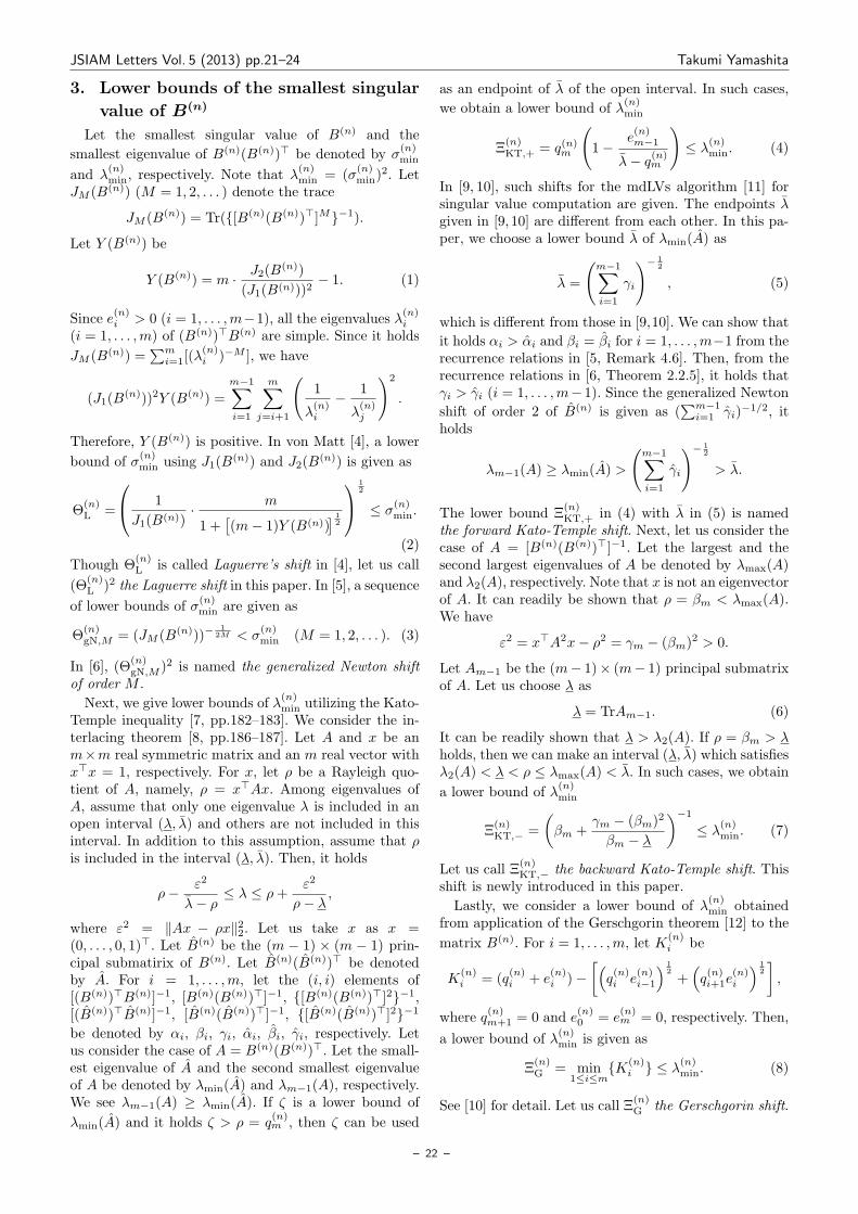
JSIAM Letters Vol. 5 (2013) pp.21–24 Takumi Yamashita
3. Lower bounds of the smallest singular
value of B(n)
Let the smallest singular value of B(n) and the
smallest eigenvalue of B(n)(B(n))⊤ be denoted by σ(n)min
and λ(n)min, respectively. Note that λ
(n)min = (σ
(n)min)
2. LetJM (B(n)) (M = 1, 2, . . . ) denote the trace
JM (B(n)) = Tr([B(n)(B(n))⊤]M−1).
Let Y (B(n)) be
Y (B(n)) = m · J2(B(n))
(J1(B(n)))2− 1. (1)
Since e(n)i > 0 (i = 1, . . . ,m−1), all the eigenvalues λ
(n)i
(i = 1, . . . ,m) of (B(n))⊤B(n) are simple. Since it holds
JM (B(n)) =∑mi=1[(λ
(n)i )−M ], we have
(J1(B(n)))2Y (B(n)) =
m−1∑i=1
m∑j=i+1
(1
λ(n)i
− 1
λ(n)j
)2
.
Therefore, Y (B(n)) is positive. In von Matt [4], a lower
bound of σ(n)min using J1(B
(n)) and J2(B(n)) is given as
Θ(n)L =
1
J1(B(n))· m
1 +[(m− 1)Y (B(n))
] 12
12
≤ σ(n)min.
(2)
Though Θ(n)L is called Laguerre’s shift in [4], let us call
(Θ(n)L )2 the Laguerre shift in this paper. In [5], a sequence
of lower bounds of σ(n)min are given as
Θ(n)gN,M = (JM (B(n)))−
12M < σ
(n)min (M = 1, 2, . . . ). (3)
In [6], (Θ(n)gN,M )2 is named the generalized Newton shift
of order M .
Next, we give lower bounds of λ(n)min utilizing the Kato-
Temple inequality [7, pp.182–183]. We consider the in-terlacing theorem [8, pp.186–187]. Let A and x be anm×m real symmetric matrix and an m real vector withx⊤x = 1, respectively. For x, let ρ be a Rayleigh quo-tient of A, namely, ρ = x⊤Ax. Among eigenvalues ofA, assume that only one eigenvalue λ is included in anopen interval (λ, λ) and others are not included in thisinterval. In addition to this assumption, assume that ρis included in the interval (λ, λ). Then, it holds
ρ− ε2
λ− ρ≤ λ ≤ ρ+ ε2
ρ− λ,
where ε2 = ∥Ax − ρx∥22. Let us take x as x =(0, . . . , 0, 1)⊤. Let B(n) be the (m − 1) × (m − 1) prin-cipal submatirix of B(n). Let B(n)(B(n))⊤ be denotedby A. For i = 1, . . . ,m, let the (i, i) elements of[(B(n))⊤B(n)]−1, [B(n)(B(n))⊤]−1, [B(n)(B(n))⊤]2−1,[(B(n))⊤B(n)]−1, [B(n)(B(n))⊤]−1, [B(n)(B(n))⊤]2−1
be denoted by αi, βi, γi, αi, βi, γi, respectively. Letus consider the case of A = B(n)(B(n))⊤. Let the small-est eigenvalue of A and the second smallest eigenvalueof A be denoted by λmin(A) and λm−1(A), respectively.We see λm−1(A) ≥ λmin(A). If ζ is a lower bound of
λmin(A) and it holds ζ > ρ = q(n)m , then ζ can be used
as an endpoint of λ of the open interval. In such cases,
we obtain a lower bound of λ(n)min
Ξ(n)KT,+ = q(n)m
(1−
e(n)m−1
λ− q(n)m
)≤ λ(n)min. (4)
In [9, 10], such shifts for the mdLVs algorithm [11] forsingular value computation are given. The endpoints λgiven in [9, 10] are different from each other. In this pa-per, we choose a lower bound λ of λmin(A) as
λ =
(m−1∑i=1
γi
)− 12
, (5)
which is different from those in [9,10]. We can show that
it holds αi > αi and βi = βi for i = 1, . . . ,m−1 from therecurrence relations in [5, Remark 4.6]. Then, from therecurrence relations in [6, Theorem 2.2.5], it holds thatγi > γi (i = 1, . . . ,m− 1). Since the generalized Newton
shift of order 2 of B(n) is given as (∑m−1i=1 γi)
−1/2, itholds
λm−1(A) ≥ λmin(A) >
(m−1∑i=1
γi
)− 12
> λ.
The lower bound Ξ(n)KT,+ in (4) with λ in (5) is named
the forward Kato-Temple shift. Next, let us consider thecase of A = [B(n)(B(n))⊤]−1. Let the largest and thesecond largest eigenvalues of A be denoted by λmax(A)and λ2(A), respectively. Note that x is not an eigenvectorof A. It can readily be shown that ρ = βm < λmax(A).We have
ε2 = x⊤A2x− ρ2 = γm − (βm)2 > 0.
Let Am−1 be the (m− 1)× (m− 1) principal submatrixof A. Let us choose λ as
λ = TrAm−1. (6)
It can be readily shown that λ > λ2(A). If ρ = βm > λholds, then we can make an interval (λ, λ) which satisfiesλ2(A) < λ < ρ ≤ λmax(A) < λ. In such cases, we obtain
a lower bound of λ(n)min
Ξ(n)KT,− =
(βm +
γm − (βm)2
βm − λ
)−1
≤ λ(n)min. (7)
Let us call Ξ(n)KT,− the backward Kato-Temple shift. This
shift is newly introduced in this paper.
Lastly, we consider a lower bound of λ(n)min obtained
from application of the Gerschgorin theorem [12] to the
matrix B(n). For i = 1, . . . ,m, let K(n)i be
K(n)i = (q
(n)i + e
(n)i )−
[(q(n)i e
(n)i−1
) 12
+(q(n)i+1e
(n)i
) 12
],
where q(n)m+1 = 0 and e
(n)0 = e
(n)m = 0, respectively. Then,
a lower bound of λ(n)min is given as
Ξ(n)G = min
1≤i≤mK(n)
i ≤ λ(n)min. (8)
See [10] for detail. Let us call Ξ(n)G the Gerschgorin shift.
– 22 –

JSIAM Letters Vol. 5 (2013) pp.21–24 Takumi Yamashita
4. A new shift strategy
In this section, we present a shift strategy for the dqdsalgorithm. In this strategy, we prepare a “flag”. Accord-ing to value of this flag, we compute a shift in differentways. At the start of singular value computation, thevalue of this flag is set to “0”. Note that the subroutineDLASQ in LAPACK has a function to detect failure ofthe Cholesky transform with shift. This failure occurs inthe following cases:
• The computed shift is no less than the minimal
eigenvalue λ(n)min of B(n)(B(n))⊤.
• The computed shift is smaller than λ(n)min but very
close to it.
When the flag is “0” and this failure occures, the flagis changed to “1” before beginning of the next itera-tion. The flag “1” is reset to “0” when only deflationoccurs. Regardless the value of the flag, when failureof the Cholesky transform with shift occurs, our imple-mentation uses the original retry strategy implementedin LAPACK.In the case where the value of the flag is “0”, we de-
termine shift as maxΘ1,Θ2,Θ3, where Θi (i = 1, 2, 3)are given as follows.
• Setting of Θ1: The quantity Y (B(n)), which is the-oretically positive, in (1) is computed. When nu-merically computed Y (B(n)) is positive, we com-
pute (Θ(n)L )2 according to (2) and set Θ1 =
(Θ(n)L )2. When numerically computed Y (B(n)) is
non-positive, we compute (Θ(n)gN,M )2 for M = 2 ac-
cording to (3) and set Θ1 = (Θ(n)gN,2)
2.
• Setting of Θ2: We compute λ in (5). If λ > q(n)m
holds, then we compute Ξ(n)KT,+ in (4) and set Θ2 =
Ξ(n)KT,+. Else, we set Θ2 = 0.
• Setting of Θ3: If λ ≥ βm, then we set Θ3 = 0. If thequantity γm− (βm)2, which is theoretically positivefrom (1), is numerically non-positive, then we setΘ3 = 0. If λ < βm holds and numerically computed
γm − (βm)2 is positive, then we compute Ξ(n)KT,− in
(7) and set Θ3 = Ξ(n)KT,−.
In the case where the value of the flag is “1”, we com-
pute the lower bound Ξ(n)G in (8). If Ξ
(n)G is positive, then
we use it as a shift. Else, we do not execute shift of origin,namely, shift is zero.An efficient method to compute quantities λ in (5),
J1(B(n)) and J2(B
(n)) is required. The diagonals of[B(n)(B(n))T ]−1 and [B(n)(B(n))T ]2−1 can be ob-tained through simple recurrence relations. These recur-rence relations are found in [5, 6].
5. Numerical experiment
In this section, performance of the dqds algorithmwith the new shift strategy introduced in the previoussection is compared with that of DLASQ in LAPACK3.4.0. We use a computer with the Intel(R) CoreTM [email protected] CPU, 8 GB of memory, Linux operating
system and gfortran version 4.4.5 compiler. We compileour source code with option -O2.As input upper bidiagonal matrices, we prepare ran-
dom matrices and precision test matrices. The randommatrices are upper bidiagonal matrices where all the di-agonals and the upper subdiagonals are given from uni-form pseudo-random numbers in interval [0, 1]. The pre-cision test matrices are upper bidiagonal matrices whereall the diagonals and the upper subdiagonals are 1. Them×m precision test matrix has the same singular valueswith the m ×m upper bidiagonal matrix Bm where allthe diagonals and the upper subdiagonals are 1 and −1,respectively. It is well-known that the matrix Bm hassingular values expressed by a trigonometric function as
σi = 2 sin
(2i− 1
2(2m+ 1)π
)(i = 1, . . . ,m).
Since singular values of the precision test matrices areexactly given, we can evaluate relative errors of com-puted singular values of these matrices.Our shift strategy is implemented into the dqds al-
gorithm by replacing the aggressive shift in DLASQ.The deflation, splitting and stopping criteria are samein both implementations. Moreover, the scaling strategyin DLASQ is also changed in our implementation. In thischange, scaling size is changed to be smaller. Possibilityof underflow becomes smaller according to increase ofscaling size [3]. Therefore, our change of scaling strategyis fair.Results of experiment are shown in Tables from 1 to
7. On the random matrices, we prepare 10 matrices foreach size. Numerical computation is executed once foreach matrix. Data of performance are averages amongthe 10 matrices. On the precision test matrices, numeri-cal computation is executed once for each size of matrix.Errors of singular values shown in Table 5 are averagesof absolute values of relative errors on all the singularvalues. Note that we executed numerical computationsfor Tables from 1 to 5 and for Tables 6 and 7 indepen-dently. Each column for percentage in Tables 6 and 7represents zero shift, the Laguerre shift, the generalizedNewton shift of order 2, the forward Kato-Temple shift,the backward Kato-Temple shift and the Gerschgorinshift, respectively.We see that
• In all the cases, iteration numbers in our strategyare less than those in DLASQ.
• On the random matrices, except for the case wherethe matrix size is 10000, the averages of execu-tion time in our strategy are shorter than those inDLASQ.
• On the precision test matrices, execution time inour strategy is longer than that in DLASQ in all thecases. While, the relative errors of the computed sin-gular values in our strategy are smaller than thosein DLASQ in all the cases.
On tables from 1 to 4, reversal between the numbersof iterations and the execution time is caused from fre-quency of splitting.
– 23 –
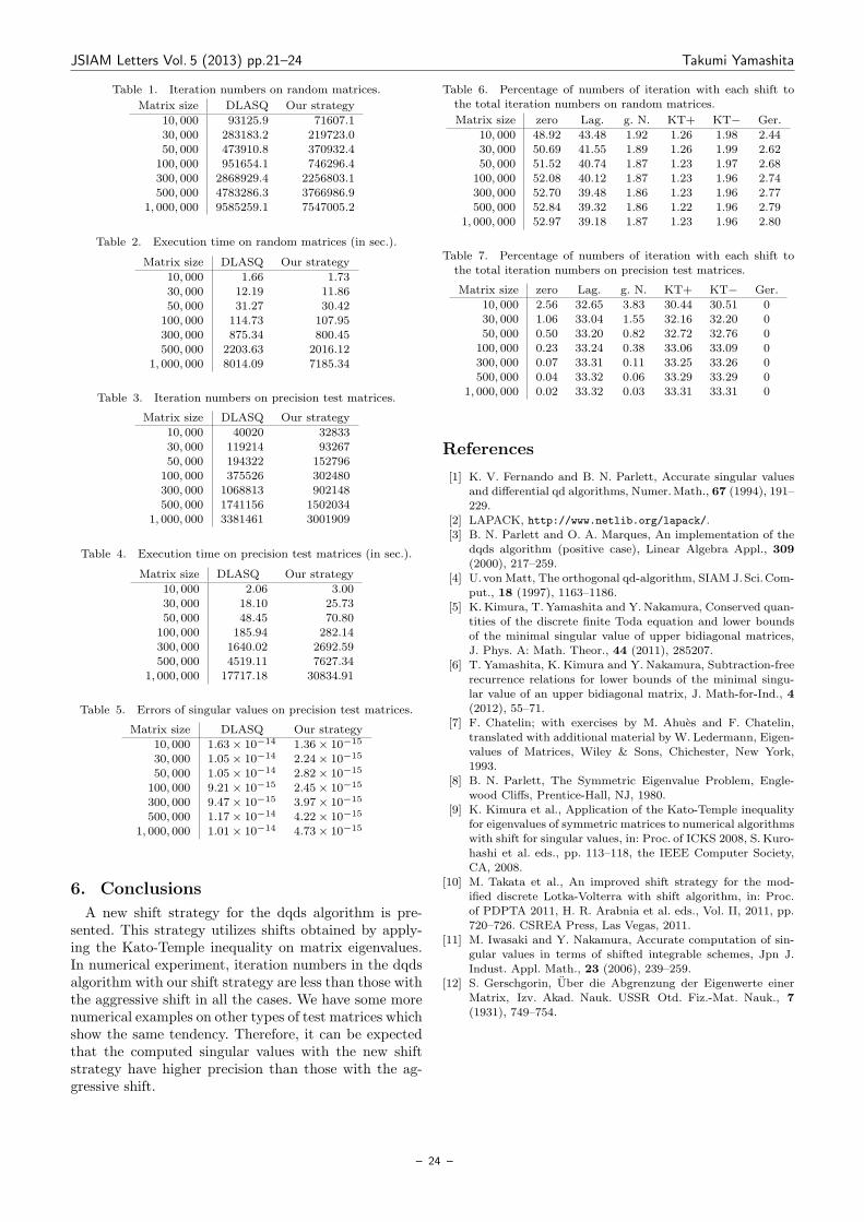
JSIAM Letters Vol. 5 (2013) pp.21–24 Takumi Yamashita
Table 1. Iteration numbers on random matrices.
Matrix size DLASQ Our strategy
10, 000 93125.9 71607.130, 000 283183.2 219723.050, 000 473910.8 370932.4
100, 000 951654.1 746296.4300, 000 2868929.4 2256803.1500, 000 4783286.3 3766986.9
1, 000, 000 9585259.1 7547005.2
Table 2. Execution time on random matrices (in sec.).
Matrix size DLASQ Our strategy
10, 000 1.66 1.73
30, 000 12.19 11.8650, 000 31.27 30.42
100, 000 114.73 107.95300, 000 875.34 800.45
500, 000 2203.63 2016.121, 000, 000 8014.09 7185.34
Table 3. Iteration numbers on precision test matrices.
Matrix size DLASQ Our strategy
10, 000 40020 32833
30, 000 119214 9326750, 000 194322 152796
100, 000 375526 302480300, 000 1068813 902148
500, 000 1741156 15020341, 000, 000 3381461 3001909
Table 4. Execution time on precision test matrices (in sec.).
Matrix size DLASQ Our strategy
10, 000 2.06 3.0030, 000 18.10 25.7350, 000 48.45 70.80
100, 000 185.94 282.14300, 000 1640.02 2692.59500, 000 4519.11 7627.34
1, 000, 000 17717.18 30834.91
Table 5. Errors of singular values on precision test matrices.
Matrix size DLASQ Our strategy
10, 000 1.63× 10⁻¹⁴ 1.36× 10⁻¹⁵
30, 000 1.05× 10⁻¹⁴ 2.24× 10⁻¹⁵
50, 000 1.05× 10⁻¹⁴ 2.82× 10⁻¹⁵
100, 000 9.21× 10⁻¹⁵ 2.45× 10⁻¹⁵
300, 000 9.47× 10⁻¹⁵ 3.97× 10⁻¹⁵
500, 000 1.17× 10⁻¹⁴ 4.22× 10⁻¹⁵
1, 000, 000 1.01× 10⁻¹⁴ 4.73× 10⁻¹⁵
6. Conclusions
A new shift strategy for the dqds algorithm is pre-sented. This strategy utilizes shifts obtained by apply-ing the Kato-Temple inequality on matrix eigenvalues.In numerical experiment, iteration numbers in the dqdsalgorithm with our shift strategy are less than those withthe aggressive shift in all the cases. We have some morenumerical examples on other types of test matrices whichshow the same tendency. Therefore, it can be expectedthat the computed singular values with the new shiftstrategy have higher precision than those with the ag-gressive shift.
Table 6. Percentage of numbers of iteration with each shift tothe total iteration numbers on random matrices.
Matrix size zero Lag. g. N. KT+ KT− Ger.
10, 000 48.92 43.48 1.92 1.26 1.98 2.4430, 000 50.69 41.55 1.89 1.26 1.99 2.62
50, 000 51.52 40.74 1.87 1.23 1.97 2.68100, 000 52.08 40.12 1.87 1.23 1.96 2.74300, 000 52.70 39.48 1.86 1.23 1.96 2.77500, 000 52.84 39.32 1.86 1.22 1.96 2.79
1, 000, 000 52.97 39.18 1.87 1.23 1.96 2.80
Table 7. Percentage of numbers of iteration with each shift to
the total iteration numbers on precision test matrices.
Matrix size zero Lag. g. N. KT+ KT− Ger.
10, 000 2.56 32.65 3.83 30.44 30.51 0
30, 000 1.06 33.04 1.55 32.16 32.20 050, 000 0.50 33.20 0.82 32.72 32.76 0
100, 000 0.23 33.24 0.38 33.06 33.09 0300, 000 0.07 33.31 0.11 33.25 33.26 0
500, 000 0.04 33.32 0.06 33.29 33.29 01, 000, 000 0.02 33.32 0.03 33.31 33.31 0
References
[1] K. V. Fernando and B. N. Parlett, Accurate singular valuesand differential qd algorithms, Numer.Math., 67 (1994), 191–229.
[2] LAPACK, http://www.netlib.org/lapack/.[3] B. N. Parlett and O. A. Marques, An implementation of the
dqds algorithm (positive case), Linear Algebra Appl., 309(2000), 217–259.
[4] U.von Matt, The orthogonal qd-algorithm, SIAM J.Sci.Com-put., 18 (1997), 1163–1186.
[5] K. Kimura, T. Yamashita and Y.Nakamura, Conserved quan-tities of the discrete finite Toda equation and lower bounds
of the minimal singular value of upper bidiagonal matrices,J. Phys. A: Math. Theor., 44 (2011), 285207.
[6] T. Yamashita, K. Kimura and Y. Nakamura, Subtraction-free
recurrence relations for lower bounds of the minimal singu-lar value of an upper bidiagonal matrix, J. Math-for-Ind., 4(2012), 55–71.
[7] F. Chatelin; with exercises by M. Ahues and F. Chatelin,
translated with additional material by W. Ledermann, Eigen-values of Matrices, Wiley & Sons, Chichester, New York,1993.
[8] B. N. Parlett, The Symmetric Eigenvalue Problem, Engle-
wood Cliffs, Prentice-Hall, NJ, 1980.[9] K. Kimura et al., Application of the Kato-Temple inequality
for eigenvalues of symmetric matrices to numerical algorithmswith shift for singular values, in: Proc. of ICKS 2008, S. Kuro-
hashi et al. eds., pp. 113–118, the IEEE Computer Society,CA, 2008.
[10] M. Takata et al., An improved shift strategy for the mod-ified discrete Lotka-Volterra with shift algorithm, in: Proc.
of PDPTA 2011, H. R. Arabnia et al. eds., Vol. II, 2011, pp.720–726. CSREA Press, Las Vegas, 2011.
[11] M. Iwasaki and Y. Nakamura, Accurate computation of sin-
gular values in terms of shifted integrable schemes, Jpn J.Indust. Appl. Math., 23 (2006), 239–259.
[12] S. Gerschgorin, Uber die Abgrenzung der Eigenwerte einerMatrix, Izv. Akad. Nauk. USSR Otd. Fiz.-Mat. Nauk., 7
(1931), 749–754.
– 24 –

JSIAM Letters Vol.5 (2013) pp.25–28 c⃝2013 Japan Society for Industrial and Applied Mathematics J S I A MLetters
Convergence analysis of accurate inverse
Cholesky factorization
Yuka Yanagisawa1 and Takeshi Ogita1
1 Tokyo Woman’s Christian University, 2-6-1 Zempukuji, Suginami-ku, Tokyo 167-8585, Japan
E-mail d11m002 cis.twcu.ac.jp
Received October 30, 2012, Accepted November 11, 2012
Abstract
This paper is concerned with factorization of symmetric and positive definite matrices whichare extremely ill-conditioned. Recently, Ogita and Oishi derived an iterative algorithm for anaccurate inverse matrix factorization based on Cholesky factorization for such ill-conditionedmatrices. We analyze the behavior of the algorithm in detail and explain its convergency bythe use of numerical error analysis. Main analysis is that each iteration reduces the conditionnumber of a preconditioned matrix by a factor around the relative rounding error unit untilconvergence, which is consistent with the existing numerical results.
Keywords convergence analysis, Cholesky factorization, ill-conditioned matrix, conditionnumber, accurate numerical algorithm
Research Activity Group Quality of Computations
1. Introduction
Let R be the set of real numbers, and F a set offloating-point numbers conforming IEEE standard 754.Denote by u the relative rounding error unit of floating-point arithmetic. In double precision (binary64) arith-metic, u = 2−53 ≈ 1.1 × 10⁻¹⁶. Throughout this paper,assume that neither overflow nor underflow occurs. ForA ∈ Rn×n define κ(A) := ∥A∥∥A−1∥ as the conditionnumber of A, where ∥ · ∥ stands for spectral norm formatrices and Euclidean norm for vectors.In this paper, we consider to treat the case where
A is symmetric, positive definite and extremely ill-conditioned such that
κ(A)≫ u−1. (1)
Let A ∈ Fn×n with (1). When using Cholesky fac-torization to obtain a computed solution x of Ax = bwith b ∈ Fn by floating-point arithmetic, few or no cor-rect digit can be expected for x. However, using Ogita-Oishi’s algorithm [1], we can calculate a good approxi-mate inverse X of the exact Cholesky factor R such thatA = RT R satisfying κ(XAXT ) ≈ 1, and A−1 ≈ XXT .Thus, the Ogita-Oishi’s algorithm can give an accuratenumerical solution of x ≈ XXT b.We analyze the behavior of the algorithm in detail
and explain its convergency by the use of numerical er-ror analysis. Main analysis to be explained is that eachiteration of the Ogita-Oishi’s algorithm reduces the con-dition number of a preconditioned matrix by a factoraround n2u until convergence, which is consistent withthe numerical results [1]. The key of the analysis is inmultiplicative corrections of an approximate inverse Xof R. The Ogita-Oishi’s algorithm requires an algorithmfor accurate dot product, which helps to treat extremelyill-conditioned matrices. Moreover, we show it is impor-
tant to choose adequate computational precision for cal-culating dot products.
2. Notation and definitions
For A = (aij), B = (bij) ∈ Rn×n, we denote by|A| = (|aij |) ∈ Rn×n a nonnegative matrix consistingof entrywise absolute values, and an inequality A ≤ Bis understood entrywise, i.e., aij ≤ bij for all (i, j). Thenotation A ≥ O means that all elements of A are non-negative. Similar notation applies to real vectors. Let Idenote the identity matrix.The trace of A = (aij) ∈ Rn×n is defined by
tr(A) :=
n∑i=1
aii.
The inversion of an upper triangular matrix R ∈ Fn×nin solving a matrix equation RT = I for T using astandard numerical algorithm (e.g., xTRSV in BLAS andxTRTRI in LAPACK) is defined by
T := triinv(R).
For readability we denote by φ(γ) a constant such asφ(γ) = c · γ where c := O(1) with 0 < c≪ u−1.Let FΣ be a set of sum of floating-point numbers such
that
FΣ =
x ∈ R : x =
m∑i=1
xi, xi ∈ F,m ∈ N
.
Note that F ⊆ FΣ ⊂ R.Let A,B ∈ Fn×nΣ . Assume that we have a function of
calculating C ∈ Fn×nΣ , for any k, l ∈ N, l ≤ k satisfying
|AB − C| ≤ φ(ul)|AB|+ φ(uk)|A||B|. (2)
Note that C =∑li=1 Ci with Ci ∈ Fn×n, i = 1, 2, . . . , l.
– 25 –

JSIAM Letters Vol. 5 (2013) pp.25–28 Yuka Yanagisawa et al.
Namely, C is an approximation of AB as if computedin k-fold working precision and rounded into l piecesof working precision floating-point numbers. We denotesuch a function as
C1:l = ABlk. (3)
Such accurate dot product algorithms satisfying (2) havebeen proposed in [2–4].Let ⟨AM , AR⟩ denote an interval matrix of the
midpoint-radius representation such that
⟨AM , AR⟩ :=X ∈ Rn×n : |X −AM | ≤ AR
with a midpoint AM ∈ Fn×n and a radius AR ∈ Fn×n,AR ≥ O.Similar notation in (3) applies to BTAB, i.e.,
⟨D,E⟩ =BTAB
1k
which satisfies
E ≤ φ(u)|BTAB|+ φ(uk)|BT ||A||B| (4)
for D ∈ Fn×n with D = DT , E ∈ Fn×n, E ≥ O.For later use, we define shift(A) for A ∈ Fn×n by
shift(A) := cnu · tr(A), cn =n+ 1
1− (n+ 1)(n+ 2)u.
3. Accurate and robust inverse Cholesky
factorization
Let A = AT ∈ Fn×n with aii > 0 for 1 ≤ i ≤ n.Suppose a standard numerical Cholesky factorization ofA runs to completion. Here “run to completion” meansthat no imaginary root appears in the factorization pro-cess. Throughout the paper, the Matlab-style notationR = chol(A) means a floating-point Cholesky factoriza-tion of A using a standard numerical algorithm (e.g.,xPOTRF in LAPACK) such that A ≈ RTR where R is anupper triangular matrix.Suppose the exact Cholesky factorization of A runs to
completion such that A = RT R. Then it holds that
κ(R) = κ(A)12 . (5)
Let R be a computed Cholesky factor of A + δI ∈Fn×n for some suitable δ > 0, i.e., R = chol(A+ δI). Ifκ(A) ≳ u−1, then κ(A+δI) is down to φ(α−1) in almostall cases. Thus,
κ(R) ≈ min(κ(A), φ(α−1))12 (6)
follows. For more detail, see [1].As long as A is positive definite, chol(A + δI) never
breaks down, even if taking the rounding errors into ac-count [6]. For δ := shift(A), define ∆ := (A+δI)−RT R,then ∥∆∥ ≤ δ. For n≪ u−1, cn ≈ n and
∥∆∥ ≈ nu · tr(A). (7)
The following is an algorithm for an accurate inverseCholesky factorization:
Algorithm 1 (Ogita-Oishi [1]) For a symmetricmatrix A = (aij) ∈ Fn×nΣ with aii > 0 for all i and aspecified tolerance εtol ≤ 1, the following algorithm cal-
culates an upper triangular matrix X(k)1:mk
∈ Fn×nΣ such
that ∥X(k)T1:mk
AX(k)1:mk
− I∥ ≲ εtol.
k = 0, G(0) := A,E(0) := O,X01:1 := I
repeat
k = k + 1
δk := shift(G(k−1)) + ∥E(k−1)∥ (8)
Compute S(k−1) ∈ Fn×n withS(k−1)ii ≥ G(k−1)
ii + δk
S(k−1)ij = G
(k−1)ij for i = j
.
R(k) := chol(S(k−1)) (9)
T (k) := triinv(R(k)) (10)
X(k)1:mk
:=X
(k−1)1:mk−1
T (k)mk
mk
% mk :=⌈k2
⌉+ 1
⟨G(k), E(k)⟩ :=X
(k)T1:mk
AX(k)1:mk
1
k+1(11)
until ∥G(k) − I∥ ≤ εtol (12)
Remark 2 If it holds that ∥E(k−1)∥ ≈ u∥G(k−1)∥, then
δk := cnu · tr(G(k−1)) + ∥E(k−1)∥ ≈ n2u∥G(k−1)∥.
If that is the case, then we have α ≈ n2u. Note thatS(k−1) ≈ G(k−1) + δkI, so that we use G(k−1) + δkIinstead of S(k−1) in the following analysis.
4. Analysis
We present the following lemmas for error bounds onan inversion of a triangular matrix.
Lemma 3 (Higham [5, Lemma 14.1]) Let R ∈Fn×n be a triangular matrix. Let X := triinv(R). Then
|I −RX| ≤ φ(u)|R||X|.
Lemma 4 Let R and X be defined as in Lemma 3.Then
∥I −XTRTRX∥ ≤ 2β + β2
where β := φ(u)∥ |R||X| ∥.We omit the proof of Lemma 4 in this paper. If β ≲ 1satisfies, then β2 ≲ 1 and
∥I −XTRTRX∥ ≲ φ(u)∥R∥∥X∥. (13)
Next, we introduce a Rump’s lemma for an estimationof a norm of a matrix.
Lemma 5 (Rump [7, Lemma 3.7]) Let a matrixA ∈ Rn×n and a vector x ∈ Rn be given which are notcorrelated. Suppose n ≥ 4. Then
∥A∥ ≥ E(∥Ax∥∥x∥
)≥ 0.61
(n− 1)12
∥A∥,
where E(·) denotes an expectation value.
This implies ∥A∥∥x∥ ≈ ∥Ax∥ in general.Similarly to [7, Observation 3.6], we present the fol-
lowing observation.
Observation 6 Let A = AT ∈ Fn×n with aii > 0for 1 ≤ i ≤ n. Let a triangular matrix R ∈ Fn×n be a
– 26 –
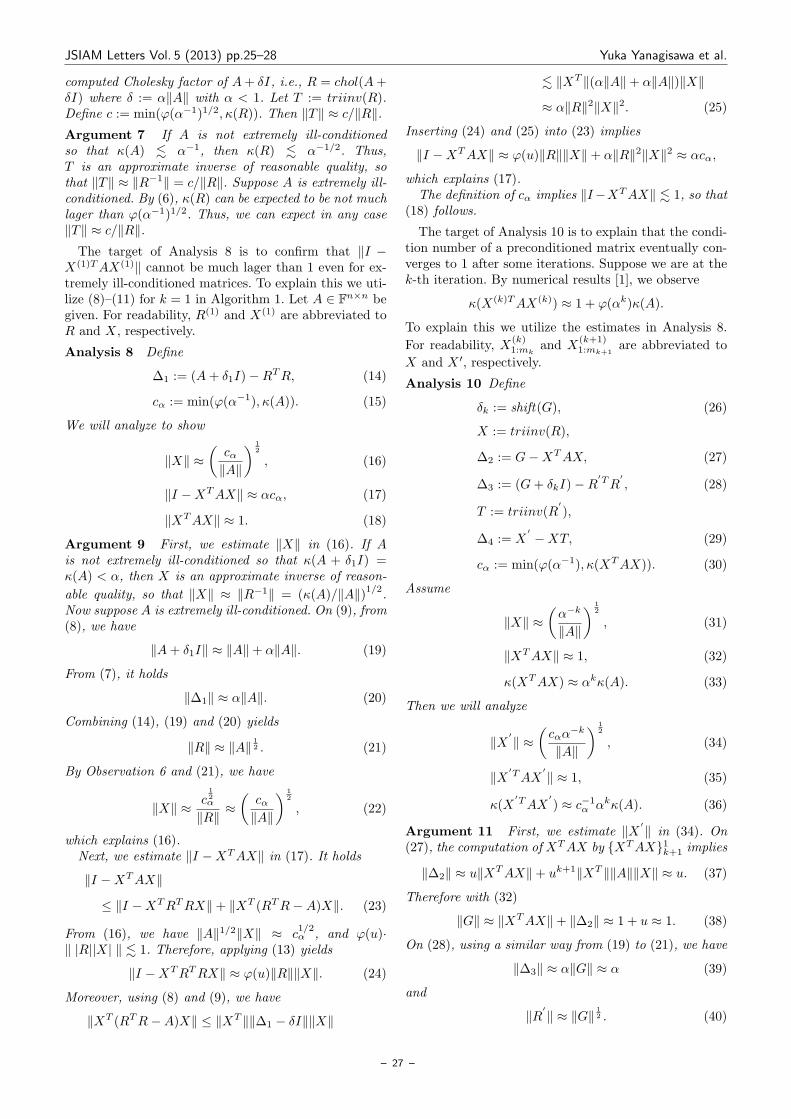
JSIAM Letters Vol. 5 (2013) pp.25–28 Yuka Yanagisawa et al.
computed Cholesky factor of A+ δI, i.e., R = chol(A+δI) where δ := α∥A∥ with α < 1. Let T := triinv(R).Define c := min(φ(α−1)1/2, κ(R)). Then ∥T∥ ≈ c/∥R∥.Argument 7 If A is not extremely ill-conditionedso that κ(A) ≲ α−1, then κ(R) ≲ α−1/2. Thus,T is an approximate inverse of reasonable quality, sothat ∥T∥ ≈ ∥R−1∥ = c/∥R∥. Suppose A is extremely ill-conditioned. By (6), κ(R) can be expected to be not muchlager than φ(α−1)1/2. Thus, we can expect in any case∥T∥ ≈ c/∥R∥.The target of Analysis 8 is to confirm that ∥I −
X(1)TAX(1)∥ cannot be much lager than 1 even for ex-tremely ill-conditioned matrices. To explain this we uti-lize (8)–(11) for k = 1 in Algorithm 1. Let A ∈ Fn×n begiven. For readability, R(1) and X(1) are abbreviated toR and X, respectively.
Analysis 8 Define
∆1 := (A+ δ1I)−RTR, (14)
cα := min(φ(α−1), κ(A)). (15)
We will analyze to show
∥X∥ ≈(cα∥A∥
) 12
, (16)
∥I −XTAX∥ ≈ αcα, (17)
∥XTAX∥ ≈ 1. (18)
Argument 9 First, we estimate ∥X∥ in (16). If Ais not extremely ill-conditioned so that κ(A + δ1I) =κ(A) < α, then X is an approximate inverse of reason-
able quality, so that ∥X∥ ≈ ∥R−1∥ = (κ(A)/∥A∥)1/2.Now suppose A is extremely ill-conditioned. On (9), from(8), we have
∥A+ δ1I∥ ≈ ∥A∥+ α∥A∥. (19)
From (7), it holds
∥∆1∥ ≈ α∥A∥. (20)
Combining (14), (19) and (20) yields
∥R∥ ≈ ∥A∥ 12 . (21)
By Observation 6 and (21), we have
∥X∥ ≈ c12α
∥R∥≈(cα∥A∥
) 12
, (22)
which explains (16).Next, we estimate ∥I −XTAX∥ in (17). It holds
∥I −XTAX∥
≤ ∥I −XTRTRX∥+ ∥XT (RTR−A)X∥. (23)
From (16), we have ∥A∥1/2∥X∥ ≈ c1/2α , and φ(u)·
∥ |R||X| ∥ ≲ 1. Therefore, applying (13) yields
∥I −XTRTRX∥ ≈ φ(u)∥R∥∥X∥. (24)
Moreover, using (8) and (9), we have
∥XT (RTR−A)X∥ ≤ ∥XT ∥∥∆1 − δI∥∥X∥
≲ ∥XT ∥(α∥A∥+ α∥A∥)∥X∥
≈ α∥R∥2∥X∥2. (25)
Inserting (24) and (25) into (23) implies
∥I −XTAX∥ ≈ φ(u)∥R∥∥X∥+ α∥R∥2∥X∥2 ≈ αcα,
which explains (17).The definition of cα implies ∥I−XTAX∥ ≲ 1, so that
(18) follows.
The target of Analysis 10 is to explain that the condi-tion number of a preconditioned matrix eventually con-verges to 1 after some iterations. Suppose we are at thek-th iteration. By numerical results [1], we observe
κ(X(k)TAX(k)) ≈ 1 + φ(αk)κ(A).
To explain this we utilize the estimates in Analysis 8.
For readability, X(k)1:mk
and X(k+1)1:mk+1
are abbreviated to
X and X ′, respectively.
Analysis 10 Define
δk := shift(G), (26)
X := triinv(R),
∆2 := G−XTAX, (27)
∆3 := (G+ δkI)−R′TR
′, (28)
T := triinv(R′),
∆4 := X′−XT, (29)
cα := min(φ(α−1), κ(XTAX)). (30)
Assume
∥X∥ ≈(α−k
∥A∥
) 12
, (31)
∥XTAX∥ ≈ 1, (32)
κ(XTAX) ≈ αkκ(A). (33)
Then we will analyze
∥X′∥ ≈
(cαα
−k
∥A∥
) 12
, (34)
∥X′TAX
′∥ ≈ 1, (35)
κ(X′TAX
′) ≈ c−1
α αkκ(A). (36)
Argument 11 First, we estimate ∥X ′∥ in (34). On(27), the computation of XTAX by XTAX1k+1 implies
∥∆2∥ ≈ u∥XTAX∥+ uk+1∥XT ∥∥A∥∥X∥ ≈ u. (37)
Therefore with (32)
∥G∥ ≈ ∥XTAX∥+ ∥∆2∥ ≈ 1 + u ≈ 1. (38)
On (28), using a similar way from (19) to (21), we have
∥∆3∥ ≈ α∥G∥ ≈ α (39)
and
∥R′∥ ≈ ∥G∥ 1
2 . (40)
– 27 –

JSIAM Letters Vol. 5 (2013) pp.25–28 Yuka Yanagisawa et al.
Hence Observation 6 yields
∥T∥ ≈ c12α
∥R′∥≈(cα∥G∥
) 12
≈ c12α . (41)
Therefore, the computation of X′in mk-fold working
precision gives
∥∆4∥ ≈ u⌈k2 ⌉+1∥XT∥+ u⌈
k2 ⌉+1∥X∥∥T∥
≈ u⌈k2 ⌉+1
(cαα
−k
∥A∥
) 12
(42)
and with (31) and (41) it follows
∥X′∥ ≈ ∥XT∥ ≈ ∥X∥∥T∥+ ∥∆4∥ ≈
(cαα
−k
∥A∥
) 12
. (43)
Next we estimate ∥I −X ′AX
′∥. Then
∥I −X′AX
′∥
= ∥I − (XT +∆4)TA(XT +∆4)∥
≤ ∥I − TTXTAXT∥+ 2∥TTXTA∆4∥
+ ∥∆T4 A∆4∥. (44)
Here
∥I − TTXTAXT∥
= ∥(I − TTGT )− TT∆2T∥
= ∥(I − TT (R′TR
′+∆3 − δkI)T )− TT∆2T∥
≤ ∥I − TTR′TR′T∥+ ∥TT∆3T∥+ δk∥TTT∥
+ ∥TT∆2T∥. (45)
From (41), it holds ∥T∥∥R′∥ ≈ c1/2α , and
φ(u)∥ |T ||R′ | ∥ ≲ 1. Therefore, applying (13) yields
∥I − TTR′TR′T∥ ≲ φ(u)∥T∥∥R
′∥ ≈ φ(u)c
12α . (46)
Moreover, by (37)–(39) and (41), we have
∥TT∆3T∥ ≤ ∥T∥2∥∆3∥ ≈ αcα, (47)
δk∥TTT∥ = δk∥T∥2 ≈ αcα∥G∥ ≈ αcα, (48)
and
∥TT∆2T∥ ≤ ∥T∥2∥∆2∥ ≈ ucα. (49)
Inserting (46)–(49) into (45) implies
∥I − TTXTAXT∥ ≈ φ(u)c12α + αcα + αcα + ucα
≈ αcα. (50)
We estimate ∥TTXTA∆4∥ and ∥∆T4 A∆4∥ in (44). Us-
ing (37), (38), (41) and (42) yields
∥TTXTA∆4∥ = ∥TTXTAXX−1∆4∥
= ∥TT (G−∆2)X−1∆4∥
≤ ∥T∥(∥G∥+ ∥∆2∥)∥X−1∥∥∆4∥
≲ u⌈k2 ⌉+1cαα
− k2 . (51)
Moreover, by (42), it holds
∥∆T4 A∆4∥ = ∥∆4∥2∥A∥ ≈ uk+2cαα
−k. (52)
Inserting (50)–(52) into (44) implies
∥I −X′TAX
′∥ ≈ αcα + u⌈
k2 ⌉+1cαα
− k2 + uk+2cαα
−k
≈ αcα. (53)
The definition of cα implies ∥I −XTAX∥ ≲ 1, so that(35) follows.To see (36) suppose first that X is not extremely ill-
conditioned, from (27) and (37), we have κ(XTAX) <α−1. Thus, the definition (30) implies cα = κ(XTAX).By (53), κ(X
′TAX′) ≈ 1 ≈ c−1
α κ(XTAX) ≈c−1α αkκ(A) using (33). Second, suppose X is extremelyill-conditioned, the definition (30) implies cα = φ(α−1).Denote the ν-th row of X
′by x(ν), 1 ≤ ν ≤ n such that
∥X ′∥ ≈ ∥x(ν)∥. Then
∥x(ν)(RX′)−1∥ = ∥eνR−1∥ ≈ ∥R−1∥, (54)
where eν denotes the ν-th row of the identity matrix.Since X is extremely ill-conditioned, we may assumeat least one row x(ν) to be sufficiently independent of(RX
′)−1, so that Lemma 5 yields
∥(RX′)−1∥ ≈ ∥x
(ν)(RX′)−1∥
∥x(ν)∥. (55)
Inserting (34) and (54) into (55) implies
∥(RX′)−1∥ ≈ ∥R
−1∥∥X ′∥
≈ c−12
α αk2 κ(R). (56)
Therefore, from (5), (35) and (56), we have
κ(X′TAX
′) ≈ 1 · ∥(RX
′)−1∥2 ≈ c−1
α αkκ(A) (57)
which explains (36).
References
[1] T. Ogita and S. Oishi, Accurate and robust inverse Choleskyfactorization, Nonlinear Theory and Its Applications, IEICE,
3 (2012), 103–111.[2] T. Ogita, S. M. Rump and S. Oishi, Accurate sum and dot
product, SIAM J. Sci. Comput., 26 (2005), 1955–1988.[3] S. M. Rump, T. Ogita and S. Oishi, Accurate floating-point
summation part I: faithful rounding, SIAM J. Sci. Comput.,31 (2008), 189-224.
[4] S. M. Rump, T. Ogita and S. Oishi, Accurate floating-pointsummation part II: sign, K-fold faithful and rounding to near-
est, SIAM J. Sci. Comput., 31 (2008), 1269-1302.[5] N. J. Higham, Accuracy and Stability of Numerical Algo-
rithms, 2nd ed., SIAM, Philadelphia, PA, 2002.[6] S. M. Rump, Verification of positive definiteness, BIT, 46
(2006), 433-452.[7] S. M. Rump, Inversion of extremely ill-conditioned matrices
in floating-point, Jpn J. Indust. Appl. Math., 26 (2009), 249–277.
– 28 –

JSIAM Letters Vol.5 (2013) pp.29–32 c⃝2013 Japan Society for Industrial and Applied Mathematics J S I A MLetters
Error analysis of the H1 gradient method for
shape-optimization problems of continua
Daisuke Murai1 and Hideyuki Azegami1
1 Graduate School of Information Science, Nagoya University, A4-2 (780) Furo-cho, Chikusa-ku,Nagoya 464-8601, Japan
E-mail murai az.cs.is.nagoya-u.ac.jp
Received March 30, 2012, Accepted September 25, 2012
Abstract
We present an error estimation for the H1 gradient method, which provides numerical solutionsto the shape-optimization problem of the domain in which a boundary value problem isdefined. The main result is that if second-order elements are used for the solutions of themain and adjoint boundary value problems to evaluate the shape derivative, and the first-order elements are used for the solution of domain variation in the boundary value problem ofthe H1 gradient method, then we obtain first-order convergence of the solution of the domainvariation with respect to the size of the finite elements.
Keywords calculus of variations, boundary value problem, shape optimization, H1 gradientmethod, error analysis
Research Activity Group Mathematical Design
1. Introduction
Determining the optimum shape of the domain inwhich a boundary value problem of a partial differen-tial equation is defined is called a shape-optimizationproblem. A numerical solution based on the concept ofthe gradient method, and called the traction method,has been proposed [1]. In the present paper, we callthe method the H1 gradient method for the shape-optimization problem, in connection with the H1 gra-dient method for the topology optimization problem [2].Corresponding to the previous author’s work [3], thepresent paper shows the error estimation of the H1 gradi-ent method using standard finite element methods. Forsimplicity, the boundary value problem we consider inthe present paper is the Poisson problem.
2. Boundary value problem
Let Ω0 ⊂ D0 ⊂ Rd for d ∈ 2, 3 be fixed domainswith W 1,∞ and piecewise C1 class boundary ∂Ω0. Wedenote by ∂Ω−
0 the open sets on ∂Ω0 except the sets Θ0
of measure 0, which are not contained in the C1 class.Let ∂Ω0 consist of ΓD0 ∪ ΓN0 with ΓD0 ∩ ΓN0 = ∅, andlet ΓN0 be C2 class on ∂Ω−
0 . We define a set for domainmappings by
Φ =
ϕ ∈W 1,∞ (D0;Rd
) ∣∣∣∣ ess infx∈D0
ω(ϕ) > 0
, (1)
where ω(ϕ) denotes the Jacobian of ϕ with respect tox ∈ Ω0. Thus, Φ becomes a Banach space with thenorm of ∥ · ∥1,∞,D0 . Here, ∥ · ∥s,p,D0 for s ∈ [0,∞]and p ∈ [1,∞] denotes the norm on W s,p(D0;R) orW s,p(D0;Rd). Moreover, let
O =ϕ ∈ Φ
∣∣∣ ∥ϕ− ϕ0∥1,∞,D0< 1, ϕ (Ω0) ⊆ D0,
ϕ : C1class on ∂Ω−0 , C
2 class on ΓN0 ∩ ∂Ω−0
be the admissible set for domain mappings, where ϕ0 isthe identity mapping. We will use the notation Ω(ϕ) =ϕ(x) | x ∈ Ω0,ϕ ∈ O.Let b, p, and uD : D0 → R be given functions. Denot-
ing the normal by ν, ∂ν = ν ·∇, and U = H2(D0;R),we write the Poisson problem as follows. For ϕ ∈ O, findu ∈ U such that
−∆u = b in Ω(ϕ),
∂νu = p on ΓN(ϕ),
u = uD on ΓD(ϕ).
(2)
For later use, we now define the Lagrangian of (2) as
LBV(ϕ, u, v) =
∫Ω(ϕ)
(−∇u ·∇v + bv) dx+
∫ΓN(ϕ)
pv dγ
+
∫ΓD(ϕ)
[(u− uD) · ∂νv + v∂νu] dγ (3)
for u, v ∈ U , and the solution u to (2) is a stationarypoint such that LBV(ϕ, u, v) = 0 for all v ∈ U .
3. Shape-optimization problem
Let I0 and I1 denote 0, . . . ,m and 1, . . . ,m, re-spectively. For i ∈ I0, let
fi(ϕ, u) =
∫Ω(ϕ)
ζi(u) dx+
∫ΓN(ϕ)
ηiN(u) dγ
+
∫ΓD(ϕ)
ηiD(∂νu) dγ + ci (4)
be cost functions, where ζi, ηiN, and ηiD are given mapsfrom U into the function Ω(ϕ) → R, from U intoΓN(ϕ) → R, and from V = ∂νu | u ∈ U,ν on ∂Ω(ϕ)into ΓD(ϕ)→ R, respectively. Here, ci > 0 is a constant
– 29 –

JSIAM Letters Vol. 5 (2013) pp.29–32 Daisuke Murai et al.
such that fi ≤ 0 for some ϕ ∈ O. We define a shape-optimization problem as follows. Let u be the solutionto (2) for ϕ ∈ O, and fi be as defined in (4). Find ϕ,such that
minϕ∈Of0(ϕ, u) | fi(ϕ, u) ≤ 0, i ∈ I1, (2), u ∈ U . (5)
4. Shape derivative of fiLet φ be the variation of ϕ such that φ ϕ ∈ O.
We refer to the Frechet derivative of fi for i ∈ I0 withrespect to φ as the shape derivative of fi, denoted asf ′i(ϕ, u)[φ] = ⟨gi,φ⟩, and evaluated as follows. If fi is afunctional of u, (2) becomes a constraint condition forfi. Then, we define the Lagrangian for fi using (3) as
Li (ϕ, u, vi) = fi (ϕ, u) + LBV (ϕ, u, vi) , (6)
where vi ∈ U is used as the Lagrange multiplier for fi.The stationary condition of Li with respect to variationof vi is satisfied if u ∈ U is the solution of (2). On theother hand, the stationary condition of Li with respectto the variation of u is satisfied if Liu(ϕ, u, vi)[u
′] =fiu(ϕ, u)[u
′] + LBVu(ϕ, u, vi)[u′] = 0 holds for all u′ ∈
U , which is the weak form of the adjoint problem withrespect to vi ∈ U , as follows. For ϕ ∈ O and u in (2),find vi ∈ U such that
−∆vi = ζ ′i(u) in Ω(ϕ),
∂νvi = η′iN(u) on ΓN(ϕ),
vi = η′iD(∂νu) on ΓD(ϕ).
(7)
With u and vi satisfying (2) and (7), respectively, andby using the formulae for shape derivatives of domainand boundary integrals [4], we obtain
⟨gi,φ⟩ = ⟨giΩ,φ⟩+ ⟨giN,φ⟩+ ⟨giD,φ⟩ , (8)
⟨giΩ,φ⟩ =∫∂Ω(ϕ)
(ζi(u)−∇u ·∇vi + bvi)ν ·φ dγ, (9)
⟨giN,φ⟩ =∫ΓN(ϕ)
(∂ν + κ) (pvi + η′iN(u)u)ν ·φdγ
+
∫∂ΓN(ϕ)∪Θ(ϕ)
(pvi + η′iN(u)u) τ ·φdς, (10)
⟨giD,φ⟩ =∫ΓD(ϕ)
∂ν (u− uD) ∂νvi
+ ∂ν [vi − η′iD(∂νu)] ∂νuν ·φ dγ, (11)
where κ = ∇ · ν, Θ(ϕ) is the set of non-C1-class pointson ∂Ω(ϕ), and τ is the outer tangent of ΓN(ϕ)\Θ(ϕ), ifd = 3, at the same time, the normal of ∂ΓN(ϕ) ∪Θ(ϕ).
5. H1 gradient method for fiIn the context of the gradient method, −gi is used
as the direction of decreasing fi. However, in general,−gi ϕ /∈ O. Then, we use the solution φig of the H1gradient method as follows. Let X = H1(Ω(ϕ);Rd), andlet a : X×X → R be a coercive bilinear form on X suchthat there exists α > 0 that satisfies a(y,y) ≥ α∥y∥2X forall y ∈ X. For gi ∈ X ′ (dual space of X), find φig ∈ Xsuch that
a (φig,y) = −⟨gi,y⟩ (12)
for all y ∈ X. For example, we can use
a (φig,y) =
∫Ω(ϕ)
(E (φig) ·E (y) + caφig · y) dx (13)
for the bilinear form, where E(y) = (1/2) × [∇yT +(∇yT
)T], and ca is a positive constant.
6. Computation of domain variation
For problem (5), a direction that decreases f0 whilesatisfying fi(ϕ, u) ≤ 0 for i ∈ I1 is given by
φg = φ0g +∑i∈I1
λiφig (14)
using φig for i ∈ I0 in problem (12). Here, λi ∈ R fori ∈ I1 are defined as the Lagrange multipliers in thefollowing problem. For ϕ ∈ O, let gi and fi(ϕ, u) fori ∈ I1 be given. Find φ such that
minφϕ∈O
q(φ) =
1
2a(φ,φ) + ⟨g0,φ⟩
∣∣∣fi(ϕ, u) + ⟨gi,φ⟩ ≤ 0, i ∈ I1
. (15)
For problem (15), defining the Lagrangian as
LSQ (φ, λ1, . . . , λm)
= q(φ) +∑i∈I1
λi (fi(ϕ, u) + ⟨gi,φ⟩) ,
the Karush–Kuhn–Tucker conditions are given as
a(φ,y) +⟨(g0 +
∑i∈I1
λigi
),y⟩= 0, (16)
fi(ϕ, u) + ⟨gi,φ⟩ ≤ 0, i ∈ I1, (17)
λi (fi(ϕ, u) + ⟨gi,φ⟩) = 0, i ∈ I1, (18)
λi ≥ 0, i ∈ I1, (19)
for all y ϕ ∈ O. Substituting φg of (14) for φ in (16),(16) holds. If all of the constraints are active, i.e. (17)holds with the equality, we have
(⟨gi,φjg⟩)ij (λj)j = − (fi(ϕ, u) + ⟨gi,φ0g⟩)i . (20)
If g1, . . . , gm are linearly independent, (20) has a uniquesolution λi for i ∈ I1. If we begin with fi(ϕ, u) = 0 fori ∈ I1, we have
(⟨gi,φjg⟩)ij (λj)j = − (⟨gi,φ0g⟩)i . (21)
For i ∈ I1 such that λi < 0 in the solution λi to (20) or(21), setting λi = 0, removing the constraint for fi from(20) or (21), and resolving them, we have λi for i ∈ I1satisfying (16) to (19).The magnitude of φg, which means the step size for
domain variation, is adjusted by selection of ∥a∥ in prob-lem (12) using criteria, such as that of Armijo and Wolfe,to ensure global convergence in problem (5).
7. Error analysis
We estimate the error of the numerical solution to φgin (14) by the finite element method. Let Ωh = ∪Kbe a finite element approximation of Ω0 with elementsK, such that h = maxK∈K diam(K). Let ∂Ωh, ΓNh,
– 30 –
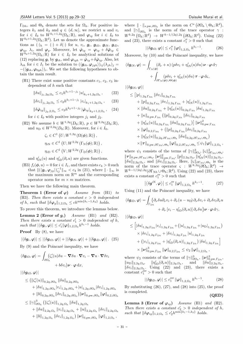
JSIAM Letters Vol. 5 (2013) pp.29–32 Daisuke Murai et al.
ΓDh, and Θh denote the sets for Ωh. For positive in-tegers k1 and k2 and q ∈ (d,∞], we restrict u and vifor i ∈ I0 to W k1+1,2q(Ωh;R), and φig for i ∈ I0 toW k2+1,2q(Ωh;Rd). Let us denote the approximate func-tions as (·)h = (·) + δ(·) for u, vi, gi, giΩ, giN, giD,φig, λi, and φg. Moreover, let φig = φig + δφig ∈W k2+1,2q(Ωh;R) for i ∈ I0 be analytical solutions of(12) replacing gi by gih, and φigh = φig+δφig. Also, letλih for i ∈ I1 be the solution to (⟨gih,φjgh⟩)ij(λjh)j =−(⟨gih,φ0gh⟩)i. We set the following hypotheses to ob-tain the main result.
(H1) There exist some positive constants c1, c2, c3 in-dependent of h such that
∥δu∥j1,2q,Ωh≤ c1hk1+1−j1 |u|k1+1,2q,Ωh
, (22)
∥δvi∥j1,2q,Ωh≤ c2hk1+1−j1 |vi|k1+1,2q,Ωh
, (23)
∥δφig∥j2,2,Ωh≤ c3hk2+1−j2 |φig|k2+1,2,Ωh
, (24)
for i ∈ I0 with positive integers j1 and j2.
(H2) We assume b ∈ W 1,2q(D0;R), p ∈ W 2,2q(D0;R),and uD ∈W 2,2q(D0;R). Moreover, for i ∈ I0,
ζi ∈ C1(U ;W 1,2q (Ω(ϕ);R)
),
ηiN ∈ C1(U ;W 2,2q (ΓN(ϕ);R)
),
ηiD ∈ C1(V ;W 2,2q (ΓD(ϕ);R)
),
and η′iN(u) and η′iD(∂νu) are given functions.
(H3) fi(ϕ, u) = 0 for i ∈ I1, and there exists c4 > 0 suchthat ∥(⟨gi,φjg⟩)−1
ij ∥∞ < c4 in (21), where ∥ · ∥∞ isthe maximum norm on Rm and the correspondingoperator norm for m×m matrices.
Then we have the following main theorem.
Theorem 1 (Error of φ) Assume from (H1) to(H3). Then there exists a constant c > 0 independentof h, such that ∥δφg∥1,2,Ωh
≤ chmink1−1,k2 holds.
To prove this theorem, we introduce the lemmas below.
Lemma 2 (Error of gi) Assume (H1) and (H2).Then there exists a constant c′1 > 0 independent of h,such that |⟨δgi,φ⟩| ≤ c′1∥φ∥1,2,Ωh
hk1−1 holds.
Proof By (8), we have
|⟨δgi,φ⟩| ≤ |⟨δgiΩ,φ⟩|+ |⟨δgiN,φ⟩|+ |⟨δgiD,φ⟩| . (25)
By (9) and the Poincare inequality, we have
⟨δgiΩ,φ⟩ =∫∂Ωh
(ζ ′i(u)δu−∇δu ·∇vi −∇u ·∇δvi
+ bδvi)ν ·φ dx,
|⟨δgiΩ,φ⟩|
≤(∥ζ ′i(u)∥0,2q,∂Ωh
∥δu∥0,2q,∂Ωh
+ |δu|1,2q,∂Ωh|vi|1,2q,∂Ωh
+|u|1,2q,∂Ωh|δvi|1,2q,∂Ωh
+ ∥b∥0,2q,∂Ωh∥δvi∥0,2q,∂Ωh
)∥ν∥0,pw,∂Ωh
∥φ∥0,2,∂Ωh
≤ ∥γ∥3∂Ωh
(∥ζ ′i(u)∥1,2q,Ωh
∥δu∥1,2q,Ωh
+ ∥δu∥2,2q,Ωh∥vi∥2,2q,Ωh
+ ∥u∥2,2q,Ωh∥δvi∥2,2q,Ωh
+ ∥b∥1,2q,Ωh∥δvi∥1,2q,Ωh
)∥ν∥0,pw,∂Ωh
∥φ∥1,2,Ωh,
where ∥ · ∥s,pw,∂Ωhis the norm on Cs
(∂Ωh \Θh;Rd
),
and ∥γ∥∂Ωhis the norm of the trace operator γ :
W k,2q(Ωh;Rd
)→ W k−1/(2q),2q
(∂Ωh;Rd
). Using (22)
and (23), there exists a constant c′′1 > 0 such that
|⟨δgiΩ,φ⟩| ≤ c′′1 ∥φ∥1,2,Ωhhk1−1. (26)
Moreover, by (10) and the Poincare inequality, we have
⟨δgiN,φ⟩ =∫ΓN(ϕ)
(∂ν + κ) (pδvi + η′iN(u)δu)ν ·φ dγ
+
∫∂ΓN(ϕ)∪Θ(ϕ)
(pδvi + η′iN(u)δu) τ ·φdς,
|⟨δgiN,φ⟩|
≤[|p|1,2q,ΓNh
∥δvi∥0,2q,ΓNh
+ ∥p∥0,2q,ΓNh|δvi|1,2q,ΓNh
+ |η′iN(u)|1,2q,ΓNh
× ∥δu∥0,2q,ΓNh+ ∥η′iN(u)∥0,2q,ΓNh
|δu|1,2q,ΓNh
+ ∥κ∥0,pw,ΓNh
(∥p∥0,2q,ΓNh
∥δvi∥0,2q,ΓNh
+ ∥η′iN(u)∥0,2q,ΓNh∥δu∥0,2q,ΓNh
)]∥ν∥20,pw,ΓNh
× ∥φ∥0,2,ΓNh+(∥p∥0,2q,ΓNh
∥δvi∥0,2q,ΓNh
+ ∥η′iN(u)∥0,2q,∂ΓNh∪Θh∥δu∥0,2q,∂ΓNh∪Θh
)×∥τ∥0,pw,∂ΓNh∪Θh
∥φ∥0,2,∂ΓNh∪Θh≤ψ1∥φ∥1,2,Ωh
,
where ψ1 consists of the terms of ∥γ∥3∂Ωh, ∥ς∥3∂ΓNh∪Θh
,
∥τ∥0,pw,∂ΓNh∪Θh, ∥ν∥20,pw,ΓNh
, ∥p∥2,2q,Ωh, ∥η′iN(u)∥2,2q,Ωh
,∥δu∥2,2q,Ωh
, and ∥δvi∥2,2q,Ωh. Here, ∥ς∥∂ΓNh∪Θh
is thenorm of the trace operator ς : W k,2q(∂Ωh;Rd) →W k−1/(2q),2q(∂ΓNh∪Θh;Rd). Using (22) and (23), thereexists a constant c′′′1 > 0 such that∣∣⟨δgiN,φ⟩∣∣ ≤ c′′′1 ∥φ∥1,2,Ωh
hk1−1. (27)
Using (11) and the Poincare inequality, we have
⟨δgiD,φ⟩ =∫ΓDh
∂νδu∂νvi+ ∂ν(u− uD) ∂νδvi+ ∂νδvi∂νu
+ ∂ν [vi − η′iD(∂νu)] ∂νδuν ·φdγ,
|⟨δgiD,φ⟩|
≤[|δu|1,2q,ΓDh
|vi|1,2q,ΓDh+(|u|1,2q,ΓDh
+|uD|1,2q,ΓDh
)× |δvi|1,2q,ΓDh
+ |δvi|1,2q,ΓDh|u|1,2q,ΓDh
+(|vi|1,2q,ΓDh
+ |η′iD(∂νu)|1,2q,ΓDh
)|δu|1,2q,ΓDh
]× ∥ν∥30,pw,ΓDh
∥φ∥0,2,ΓDh≤ ψ2 ∥φ∥1,2,Ωh
,
where ψ2 consists of the terms of ∥γ∥3∂Ωh, ∥ν∥30,pw,ΓDh
,∥uD∥2,2q,Ωh
, ∥η′iD(∂νu)∥2,2q,Ωh, and ∥δu∥2,2q,Ωh
,∥δvi∥2,2q,Ωh
. Using (22) and (23), there exists aconstant c′′′′1 > 0 such that
|⟨δgiD,φ⟩| ≤ c′′′′1 ∥φ∥1,2,Ωhhk1−1. (28)
By substituting (26), (27), and (28) into (25), the proofis completed.
(QED)
Lemma 3 (Error of φig) Assume (H1) and (H2).Then there exists a constant c′2 > 0 independent of h,such that ∥δφig∥1,2,Ωh
≤ c′2hmink1−1,k2 holds.
– 31 –
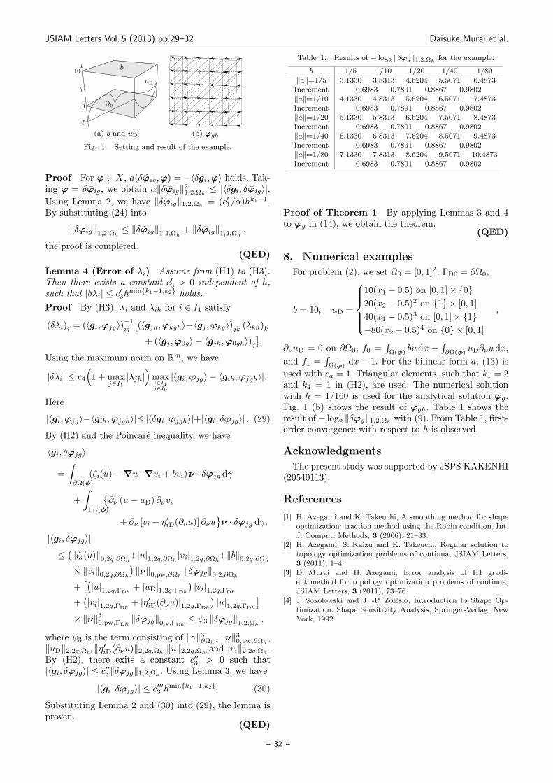
JSIAM Letters Vol. 5 (2013) pp.29–32 Daisuke Murai et al.
10
5
0
5
0
b
uD
(a) b and uD (b) φgh
Fig. 1. Setting and result of the example.
Proof For φ ∈ X, a(δφig,φ) = −⟨δgi,φ⟩ holds. Tak-ing φ = δφig, we obtain α∥δφig∥21,2,Ωh
≤ |⟨δgi, δφig⟩|.Using Lemma 2, we have ∥δφig∥1,2,Ωh
= (c′1/α)hk1−1.
By substituting (24) into
∥δφig∥1,2,Ωh≤ ∥δφig∥1,2,Ωh
+ ∥δφig∥1,2,Ωh,
the proof is completed.(QED)
Lemma 4 (Error of λi) Assume from (H1) to (H3).Then there exists a constant c′3 > 0 independent of h,such that |δλi| ≤ c′3hmink1−1,k2 holds.
Proof By (H3), λi and λih for i ∈ I1 satisfy
(δλi)i = (⟨gi,φjg⟩)−1ij
[(⟨gjh,φkgh⟩−⟨gj ,φkg⟩)jk (λkh)k+ (⟨gj ,φ0g⟩ − ⟨gjh,φ0gh⟩)j
].
Using the maximum norm on Rm, we have
|δλi| ≤ c4(1 + max
j∈I1|λjh|
)maxi∈I1j∈I0
|⟨gi,φjg⟩ − ⟨gih,φjgh⟩| .
Here
|⟨gi,φjg⟩−⟨gih,φjgh⟩|≤|⟨δgi,φjgh⟩|+|⟨gi, δφjg⟩| . (29)
By (H2) and the Poincare inequality, we have
⟨gi, δφjg⟩
=
∫∂Ω(ϕ)
(ζi(u)−∇u ·∇vi + bvi)ν · δφjg dγ
+
∫ΓD(ϕ)
∂ν (u− uD) ∂νvi
+ ∂ν [vi − η′iD(∂νu)] ∂νuν · δφjg dγ,
|⟨gi, δφjg⟩|
≤(∥ζi(u)∥0,2q,∂Ωh
+|u|1,2q,∂Ωh|vi|1,2q,∂Ωh
+∥b∥0,2q,∂Ωh
× ∥vi∥0,2q,∂Ωh
)∥ν∥0,pw,∂Ωh
∥δφjg∥0,2,∂Ωh
+[(|u|1,2q,ΓDh
+ |uD|1,2q,ΓDh
)|vi|1,2q,ΓDh
+(|vi|1,2q,ΓDh
+ |η′iD(∂νu)|1,2q,ΓDh
)|u|1,2q,ΓDh
]× ∥ν∥30,pw,ΓDh
∥δφjg∥0,2,ΓDh≤ ψ3 ∥δφjg∥1,2,Ωh
,
where ψ3 is the term consisting of ∥γ∥3∂Ωh, ∥ν∥30,pw,∂Ωh
,∥uD∥2,2q,Ωh
, ∥η′iD(∂νu)∥2,2q,Ωh, ∥u∥2,2q,Ωh
, and ∥vi∥2,2q,Ωh.
By (H2), there exits a constant c′′3 > 0 such that|⟨gi, δφjg⟩| ≤ c′′3∥δφjg∥1,2,Ωh
. Using Lemma 3, we have
|⟨gi, δφjg⟩| ≤ c′′′3 hmink1−1,k2. (30)
Substituting Lemma 2 and (30) into (29), the lemma isproven.
(QED)
Table 1. Results of − log2 ∥δφg∥1,2,Ωhfor the example.
h 1/5 1/10 1/20 1/40 1/80
∥a∥=1/5 3.1330 3.8313 4.6204 5.5071 6.4873Increment 0.6983 0.7891 0.8867 0.9802∥a∥=1/10 4.1330 4.8313 5.6204 6.5071 7.4873
Increment 0.6983 0.7891 0.8867 0.9802∥a∥=1/20 5.1330 5.8313 6.6204 7.5071 8.4873Increment 0.6983 0.7891 0.8867 0.9802∥a∥=1/40 6.1330 6.8313 7.6204 8.5071 9.4873
Increment 0.6983 0.7891 0.8867 0.9802∥a∥=1/80 7.1330 7.8313 8.6204 9.5071 10.4873Increment 0.6983 0.7891 0.8867 0.9802
Proof of Theorem 1 By applying Lemmas 3 and 4to φg in (14), we obtain the theorem.
(QED)
8. Numerical examples
For problem (2), we set Ω0 = [0, 1]2, ΓD0 = ∂Ω0,
b = 10, uD =
10(x1 − 0.5) on [0, 1]× 020(x2 − 0.5)2 on 1 × [0, 1]
40(x1 − 0.5)3 on [0, 1]× 1−80(x2 − 0.5)4 on 0 × [0, 1]
,
∂νuD = 0 on ∂Ω0, f0 =∫Ω(ϕ)
budx −∫∂Ω(ϕ)
uD∂νudx,
and f1 =∫Ω(ϕ)
dx − 1. For the bilinear form a, (13) is
used with ca = 1. Triangular elements, such that k1 = 2and k2 = 1 in (H2), are used. The numerical solutionwith h = 1/160 is used for the analytical solution φg.Fig. 1 (b) shows the result of φgh. Table 1 shows theresult of − log2 ∥δφg∥1,2,Ωh
with (9). From Table 1, first-order convergence with respect to h is observed.
Acknowledgments
The present study was supported by JSPS KAKENHI(20540113).
References
[1] H. Azegami and K. Takeuchi, A smoothing method for shapeoptimization: traction method using the Robin condition, Int.J. Comput. Methods, 3 (2006), 21–33.
[2] H. Azegami, S. Kaizu and K. Takeuchi, Regular solution to
topology optimization problems of continua, JSIAM Letters,3 (2011), 1–4.
[3] D. Murai and H. Azegami, Error analysis of H1 gradi-ent method for topology optimization problems of continua,
JSIAM Letters, 3 (2011), 73–76.[4] J. Sokolowski and J. -P. Zolesio, Introduction to Shape Op-
timization: Shape Sensitivity Analysis, Springer-Verlag, New
York, 1992.
– 32 –

JSIAM Letters Vol.5 (2013) pp.33–36 c⃝2013 Japan Society for Industrial and Applied Mathematics J S I A MLetters
Complete low-cut filter and the best constant
of Sobolev inequality
Hiroyuki Yamagishi1, Yoshinori Kametaka2, Atsushi Nagai3, Kohtaro Watanabe4
and Kazuo Takemura3
1 Tokyo Metropolitan College of Industrial Technology, 1-10-40 Higashi-ooi, Shinagawa, Tokyo140-0011, Japan
2 Osaka University, 1-3 Machikaneyama-cho, Toyonaka 560-8531, Japan3 Nihon University, 2-11-1 Shinei, Narashino 275-8576, Japan4 National Defense Academy, 1-10-20 Yokosuka 239-8686, Japan
E-mail yamagisi s.metro-cit.ac.jp
Received September 5, 2012, Accepted November 28, 2012
Abstract
We obtained the best constants of Sobolev inequalities corresponding to complete low-cutfilter. In the background, we have an n-dimensional boundary value problem and a one-dimensional periodic boundary value problem. The best constants of the correspondingSobolev inequalities are equal to diagonal values of Green’s functions for these boundaryvalue problems.
Keywords Sobolev inequality, best constant, Green’s function, Bessel function
Research Activity Group Applied Integrable Systems
1. The Sobolev inequality for a boundary
value problem in n-dimensional Eu-
clidean space
We consider the problem on the basis of a completelow-cut filter, which is a device that passes only highfrequency.We assume M = 1, 2, . . . , n = 1, 2, . . . , 2M − 1, 0 <
A <∞, x = (x1, x2, . . . , xn) ∈ Rn, ξ = (ξ1, ξ2, . . . , ξn) ∈Rn. We set the unitary inner product
⟨ξ, x⟩ =n∑j=1
ξjxj , |ξ|2 = ⟨ξ, ξ⟩.
We define Fourier transform as
u(x) −→ u(ξ) =
∫Rn
e−√−1 ⟨ξ,x⟩u(x) dx,
where dx = dx1dx2 · · · dxn. We introduce Sobolev spacewith low-cut frequency
H =u ∈WM,2 | u(ξ) = 0 (|ξ| < A)
,
Sobolev inner product
(u, v)H =
(1
2π
)n ∫|ξ|≥A
|ξ|2M u(ξ)v(ξ) dξ,
and Sobolev energy
∥u∥2H =
(1
2π
)n ∫|ξ|≥A
|ξ|2M |u(ξ)|2 dξ.
(·, ·)H is proved to be an inner product of H in Proof ofTheorem 1.H is Hilbert space with inner product (·, ·)H .Our conclusion is as follows.
Theorem 1 For any u ∈ H, there exists a positive con-stant C which is independent of u, such that a Sobolevinequality (
supy∈Rn
|u(y)|)2
≤ C ∥u∥2H (1)
holds. Among such C, the best constant is
C0 = G(0) =2
(4π)n2 Γ(n2 )(2M − n)A2M−n . (2)
If one relpaces C by C0 in the above inequality (1), theequality holds for u(x) = cG(x−y0) with arbitrary c ∈ Cand y0 ∈ Rn. Green’s function G(x, y) = G(x − y) isexplained later in Lemma 1.
In the background of this theorem, we have the fol-lowing n-dimensional boundary value problem. Concern-ing the uniqueness and existence of the solution to theboundary value problem, we have the following lemma.
Lemma 1 For an arbitrary bounded continuous func-tion f(x) satisfying the solvability condition f(ξ) =0 (|ξ| < A), the boundary value problem
BVP(−∆)Mu = f(x) (x ∈ Rn),
u(ξ) = 0 (|ξ| < A)
has a unique solution
u(x) =
∫Rn
G(x, y)f(y)dy (x ∈ Rn). (3)
G(x, y)=G(x− y) (x, y ∈ Rn) is Green’s function given
– 33 –
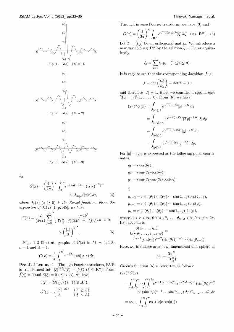
JSIAM Letters Vol. 5 (2013) pp.33–36 Hiroyuki Yamagishi et al.
-20 -10 10 20
-0.1
0.1
0.2
0.3
Fig. 1. G(x) (M = 1).
-20 -10 10 20
-0.1
0.1
0.2
0.3
Fig. 2. G(x) (M = 2).
-20 -10 10 20
-0.1
0.1
0.2
0.3
Fig. 3. G(x) (M = 3).
by
G(x) =
(1
2π
)n2∫ ∞
A
r−(2M−n)−1 (|x|r)−n−22
× Jn−22
(|x|r) dr, (4)
where Jν(z) (z ≥ 0) is the Bessel function. From theexpansion of Jν(z) [1, p.145], we have
G(x) =2
(4π)n2
∞∑j=0
[(−1)j
j!Γ(n2 +j)(2M−n−2j)A2M−n−2j
×(|x|2
)2j]. (5)
Figs. 1–3 illustrate graphs of G(x) in M = 1, 2, 3,n = 1 and A = 1.
G(x) =1
π
∫ ∞
1
r−2M cos(|x|r) dr.
Proof of Lemma 1 Through Fourier transform, BVPis transformed into |ξ|2M u(ξ) = f(ξ) (ξ ∈ Rn). From
f(ξ) = 0 and u(ξ) = 0 (|ξ| < A), we have
u(ξ) = G(ξ)f(ξ) (ξ ∈ Rn),
G(ξ) =
|ξ|−2M (|ξ| ≥ A),0 (|ξ| < A).
Through inverse Fourier transform, we have (3) and
G(x) =
(1
2π
)n ∫Rn
e√−1⟨x,ξ⟩G(ξ) dξ (x ∈ Rn). (6)
Let T = (tij) be an orthogonal matrix. We introduce anew variable y ∈ Rn by the relation ξ = Ty, or equiva-lently
ξi =n∑j=1
tijyj (1 ≤ i ≤ n).
It is easy to see that the corresponding Jacobian J is
J = det
(∂ξ
∂y
)= detT = ±1
and therefore |J | = 1. Here, we consider a special casetTx = |x|t(1, 0, . . . , 0). From (6), we have
(2π)nG(x) =
∫|ξ|≥A
e√−1 ⟨x,ξ⟩|ξ|−2M dξ
=
∫|Ty|≥A
e√−1 ⟨x,Ty⟩|Ty|−2M |J | dy
=
∫|y|≥A
e√−1 ⟨tTx,y⟩|y|−2M dy
=
∫|y|≥A
e√−1 |x|y1 |y|−2M dy.
For |y| = r, y is expressed as the following polar coordi-nates.
y1 = r cos(θ1),
y2 = r sin(θ1) cos(θ2),
y3 = r sin(θ1) sin(θ2) cos(θ3),
...
yn−2 = r sin(θ1) sin(θ2) · · · sin(θn−3) cos(θn−2),
yn−1 = r sin(θ1) sin(θ2) · · · sin(θn−2) cos(φ),
yn = r sin(θ1) sin(θ2) · · · sin(θn−2) sin(φ),
where A < r <∞, 0 < θ1, θ2, . . . , θn−2 < π, 0 < φ < 2π.Its Jacobian is
∂(y1, . . . , yn)
∂(r, θ1, . . . , θn−2, φ)=
rn−1(sin(θ1))n−2(sin(θ2))
n−3 · · · sin(θn−2).
Here, ωn is surface area of n dimensional unit sphere as
ωn =2π
n2
Γ(n2
) .Green’s function (6) is rewritten as follows:
(2π)nG(x)
=
∫ ∞
A
∫ π
0
· · ·∫ π
0
∫ 2π
0
e√−1 |x|r cos(θ1)r−(2M−n)−1(sin(θ1))
n−2
× (sin(θ2))n−3 · · · sin(θn−2) dφdθn−2 · · · dθ1dr
= ωn−1
∫ ∞
A
∫ π
0
cos (|x|r cos(θ1))
– 34 –

JSIAM Letters Vol. 5 (2013) pp.33–36 Hiroyuki Yamagishi et al.
× (sin(θ1))n−2 dθ1r
−(2M−n)−1 dr,
where we use∫ π
0
sin(|x|r cos(θ1)) (sin(θ1))n−2dθ1 = 0.
Using Lommel’s formula [1, p.179], we have
(2π)nG(x) = 2n−22 π
12Γ
(n− 1
2
)ωn−1
×∫ ∞
A
r−(2M−n)−1(|x|r)−n−22 Jn−2
2(|x|r) dr.
From
ωn−1 =Γ(n2
)π
12Γ(n−12
)ωn =2π
n−12
Γ(n−12
) ,so we have (4). Moreover, using expansion of Bessel func-tion [1, p145], we have
G(x) =2
2nπn2
×∫ ∞
A
∞∑j=0
(−1)j
j!Γ(n2 + j
)( |x|r2
)2j
r−(2M−n)−1dr.
From the assumption 2M > n, we have (5). Taking thelimit as x → 0 of (5), we have (2). Thus we provedLemma 1.
(QED)
We next show that Green’s function G(x, y) is simul-taeously a reproducing kernel for a set of Hilbert spaceH and its inner product (·, ·)H .
Lemma 2 For any u ∈ H and fixed y ∈ Rn, we havethe following reproducing relations:
u(y) = (u(x), G(x, y))H , (7)
G(0) = ∥G(x, y)∥2H . (8)
Proof of Lemma 2 Since Fourier transform ofG(x, y) = G(x− y) with respect to x is e−
√−1 ⟨ξ,y⟩G(ξ),
the relation (7) is rewritten as
(u(x), G(x, y))H
=
(1
2π
)n ∫|ξ|≥A
|ξ|2M u(ξ)e−√−1 ⟨ξ,y⟩G(ξ) dξ
=
(1
2π
)n ∫|ξ|≥A
e√−1 ⟨y,ξ⟩u(ξ) dξ = u(y).
(8) is shown by putting u(x) = G(x, y) in (7). This com-pletes the proof of Lemma 2.
(QED)
Finally, we prove Theorem 1.Proof of Theorem 1 Applying Schwarz inequality to(7) and using (8), we have
|u(y)|2 ≤ ∥G(x, y)∥2H ∥u∥2H = G(0) ∥u∥2H .
Taking the supremum with respect to y ∈ Rn, we have(supy∈Rn
|u(y)|)2
≤ G(0) ∥ux∥2H . (9)
This inequality shows that the inner product ∥u∥2H =(u, u)H is positive definite. For any fixed y0 ∈ Rn, if we
take u(x) = G(x−y0) ∈ H in the above inequality, thenwe have(
supy∈Rn
|G(y − y0)|)2
≤ G(0) ∥G(x− y0)∥2H = G(0)2.
Together with a trivial inequality
G(0)2 ≤(
supy∈Rn
|G(y − y0)|)2
,
we have(supy∈Rn
|G(y − y0)|)2
= G(0) ∥G(x− y0)∥2H .
This shows that G(0) is the best constant of (9) and theequality holds for G(x − y0). This completes the proofof Theorem 1.
(QED)
For (6), we have
|G(x)| ≤(
1
2π
)n ∫Rn
∣∣∣G(ξ)∣∣∣ dξ = G(0) (x ∈ Rn).
So we see that the maximum of G(x) is G(0).
2. The Sobolev inequality under a peri-
odic boundary condition
We here consider a one-dimensional case. For M,N =1, 2, . . . and x ∈ R, we introduce the function
φ(j, x) = e√−1 ajx,
aj = 2πj (j = 0,±1,±2, . . . ).
We define Fourier transform as
u(x) −→ u(j) =
∫ 1
0
u(x)φ(j, x) dx.
We introduce Sobolev space with periodic boundary con-dition and low-cut frequency
H =u∣∣∣u(M) ∈ L2(0, 1),
u(i)(1)− u(i)(0) = 0 (0 ≤ i ≤M − 1),
u(j) = 0 (|j| < N),
Sobolev inner product
(u, v)H =∑
|j|≥N
a2Mj u(j)v(j),
and Sobolev energy
∥u∥2H =∑
|j|≥N
a2Mj | u(j)|2 .
(·, ·)H is proved to be an inner product of H in Proof ofTheorem 2.H is Hilbert space with inner product (·, ·)H .Our conclusion is as follows.
Theorem 2 For any u ∈ H, there exists a positive con-stant C which is independent of u, such that a Sobolevinequality (
sup0≤y≤1
|u(y)|)2
≤ C∥u∥2H (10)
– 35 –

JSIAM Letters Vol. 5 (2013) pp.33–36 Hiroyuki Yamagishi et al.
holds. Among such C, the best constant is
C0 = G(0)
=
2
(2π)2Mζ(2M) (N = 1),
2
(2π)2M
ζ(2M)−N−1∑j=1
1
j2M
(N = 2, 3, . . . ),
where ζ(z) =∑∞n=1 n
−z (Rez > 1) is the well-knownRiemann-zeta function. If one relpaces C by C0 in theabove inequality (10), the equality holds for u(x) =cG(x − y0) with arbitrary c ∈ C and y0 ∈ R. Green’sfunction G(x) is explained in Lemma 3.
It should be noted that if we put N = 1 in the abovetheorem, we have Theorem 2 in our previous work [2].In the background of this theorem, we have the follow-
ing one-dimensional periodic boundary value problem.Concerning the uniqueness and existence of the solutionto the boundary value problem, we have the followinglemma.
Lemma 3 For an arbitrary bounded continuous func-tion f(x) satisfying the solvability condition f(j) = 0(|j| < N), the boundary value problem
BVP (−1)Mu(2M) = f(x) (0 < x < 1),u(i)(1)− u(i)(0) = 0 (0 ≤ i ≤ 2M − 1),u(j) = 0 (|j| < N)
has a unique solution
u(x) =
∫ 1
0
G(x, y)f(y) dy (0 < x < 1). (11)
G(x, y) = G(x − y) (0 < x, y < 1) is Green’s functiongiven by
G(x) = 2
∞∑j=N
a−2Mj cos(ajx). (12)
Proof of Lemma 3 Through Fourier transform as∑j∈Z
f(j)φ(j, x) = f(x) = (−1)Mu(2M)
= (−1)M∑j∈Z
u(j)φ(2M)(j, x) =∑j∈Z
a2Mj u(j)φ(j, x),
BVP is transformed into
a2Mj u(j) = f(j) (j ∈ Z).
From f(j) = 0 and u(j) = 0 (|j| < N), we have
u(j) = G(j)f(j) (j ∈ Z),
G(j) =
a−2Mj (|j| ≥ N),
0 (|j| < N).
Through inverse Fourier transform, we have (11) and(12) as
G(x) =∞∑
j=−∞G(j)φ(j, x) =
∑|j|≥N
a−2Mj φ(j, x)
= 2
∞∑j=N
a−2Mj cos(ajx).
We see that the maximum of G(x) is G(0). This com-pletes the proof.
(QED)
We next show that Green’s function G(x, y) is simul-taeously a reproducing kernel for a set of Hilbert spaceH and its inner product (·, ·)H .
Lemma 4 For any u ∈ H and fixed y (0 ≤ y ≤ 1), wehave the following reproducing relations.
u(y) = (u(x), G(x, y))H , (13)
G(0) = ∥G(x, y)∥2H . (14)
Proof of Lemma 4 Fourier transform of G(x, y) =
G(x−y) wiht respect to x is φ(j, y)G(j). Hence, for anyu ∈ H, we have (13) as
(u(x), G(x, y))H =∑
|j|≥N
a2Mj u(j)φ(j, y)G(j)
=∑
|j|≥N
a2Mj G(j)u(j)φ(j, y) =∑
|j|≥N
u(j)φ(j, y) = u(y).
(14) is shown by putting u(x) = G(x, y) in (13). Thiscompletes the proof of Lemma 4.
(QED)
Finally, we prove Theorem 2.Proof of Theorem 2 Applying Schwarz inequality to(13) and using (14), we have
|u(y)|2 ≤ ∥G(x, y)∥2H ∥u∥2H = G(0) ∥u∥2H .
Taking the supremum with respect to y (0 ≤ y ≤ 1), wehave (
sup0≤y≤1
|u(y)|)2
≤ G(0) ∥u∥2H . (15)
This inequality shows that the inner product ∥u∥2H =(u, u)H is positive definite. For any fixed y0 (0 ≤ y0 ≤1), if we take u(x) = G(x − y0) ∈ H in the above in-equality, then we have(
sup0≤y≤1
|G(y − y0)|)2
≤ G(0) ∥G(x− y0)∥2H = G(0)2.
Combining this and a trivial inequality
G(0)2 ≤(
sup0≤y≤1
|G(y − y0)|)2
,
we have(sup
0≤y≤1|G(y − y0)|
)2
= G(0) ∥G(x− y0)∥2H .
This shows that G(0) is the best constant of (15) and theequality holds for G(x − y0). This completes the proofof Theorem 2.
(QED)
References
[1] S.Moriguchi, K.Udagawa and S.Hitotsumatsu, Iwanami Sug-aku Koshiki III (in Japanese), Iwanami, Tokyo, 1960.
[2] Y. Kametaka et al., Riemann zeta function, Bernoulli polyno-mials and the best constant of Sobolev inequality, Sci. Math.Jpn., e-2007 (2007), 63–89.
– 36 –

JSIAM Letters Vol.5 (2013) pp.37–40 c⃝2013 Japan Society for Industrial and Applied Mathematics J S I A MLetters
A new geometric integration approach
based on local invariants
Takeru Matsuda1 and Takayasu Matsuo1
1 Department of Mathematical Informatics, Graduate School of Information Science and Tech-nology, The University of Tokyo, Hongo 7-3-1, Bunkyo-ku, Tokyo 113-0033, Japan
E-mail Takeru Matsuda mist.i.u-tokyo.ac.jp
Received October 2, 2012, Accepted December 28, 2012
Abstract
In this report we propose a simple new geometric integration approach for solving ordinary dif-ferential equations based on the concept of “local” invariants. The approach basically belongsto the class of invariants-preserving integrations, but it differs from any existing methodsin that it can automatically detect enough number of invariants, and work even for non-conservative systems. Numerical examples show that the approach can in fact work.
Keywords conservative method, local invariant, discrete gradient method
Research Activity Group Scientific Computation and Numerical Analysis
1. Introduction
In this paper, we show a simple new geometric integra-tion approach for solving ordinary differential equationsof the form:
dz
dt= f(z) (1)
where z(t) ∈ RN and f : RN → RN .ODE (1) often happens to have invariants such as en-
ergy and momentum, and for both of numerical stabilityand qualitatively better behaviors, it is generally encour-aged to employ some special integrators that preservethe invariants. The most typical integrator of this classis the discrete gradient method (see, for example, [1,2]).The method (or any similar ideas) can be, however, onlyapplied to the systems where invariants are explicitlyknown, and otherwise it is even impossible to write downthe scheme itself. Although this is not a crucial restric-tion from a practical point of view, one may still aska mathematically challenging question: is it possible topreserve even unknown invariants?It is interesting to rephrase the question in the fol-
lowing slightly different and stronger way: intuitively, ifwe know one invariant we can essentially decrease thedegree of freedom of the ODE by one. Similarly, if weknow the N − 1 (independent) invariants of ODE (1),we should be able to exactly trace the trajectory of thesolution. This is extensively discussed in the field of inte-grable systems, but we would like to remind the readersthat even for non-integrable systems it is still possibleto consider enough number of, i.e., N − 1 invariants insome weak sense that determine the trajectory. The in-variants are called “local invariants” (see, for example,[3]). It seems that this concept has not come into play inthe area of structure-preserving methods so far, to thebest of the authors’ knowledge, and that motivated ourproject below.
Our main idea in this report is to more actively utilizethe local invariants to solve ODEs. Since they are not ex-plicitly known in general, we commence by numericallydetecting them. Then we will construct a numerical inte-grator that preserves the detected invariants by the dis-crete gradient method. The numerical examples belowdemonstrates that the idea can in fact work. Note thatthis report is to raise the mathematically simple idea,and not to discuss the actual efficiency of computation.This paper is organized as follows. In Section 2 the
concept of local invariants is introduced and its conve-nient features are briefly reviewed. In Section 3 the prin-ciple of the proposed method is explained. In Section 4numerical examples are presented. Concluding remarksare given in Section 5.
2. Local Invariants
In this section the concept of local invariants is brieflyreviewed. The description is based on Chapter 2 of [3].First we review the conventional invariants—what weshould call “global invariants”—of ODE.
Definition 1 (Global invariants) A function F :RN → R is called a global invariant of ODE (1) if forall z ∈ RN and all t ∈ R,
F (ϕt(z)) = F (z), (2)
where ϕt is the flow of ODE (1).
A typical example of the global invariants is the totalenergy when the ODE is a Hamiltonian equation. Theconcept of local invariants is a weaker version of theabove definition.
Definition 2 (Local invariants) Let U be a domainin RN . A function F : U → R is called a local invariantof ODE (1) if for all z ∈ U and all t ∈ R such thatϕt(z) ∈ U ,
F (ϕt(z)) = F (z). (3)
– 37 –

JSIAM Letters Vol. 5 (2013) pp.37–40 Takeru Matsuda et al.
In order to explain the existence result of the localinvariants, let us recall the definition of the independenceof the local invariants.
Definition 3 (Independence of local invariants)Let F1, . . . , Fk be smooth real-valued functions definedon a domain U in RN . F1, . . . , Fk are called functionallydependent if for each z ∈ U there is a neighborhood Vof z and a smooth real-valued function G : Rk → R notidentically zero on any open subset of Rk, such that
G(F1(x), . . . , Fk(x)) = 0 (4)
for all x ∈ V . F1, . . . , Fk are called functionally inde-pendent if they are not functionally dependent when re-stricted to any open subset V ⊂ U .
The flow ϕt of ODE (1) can be seen as a one–dimensional Lie group acting on RN . Then, from thegeneral theory of Lie groups, we have the following the-orem.
Theorem 1 (Maximal number of independent lo-cal invariants) If ODE (1) has a unique solution, thenfor all z ∈ RN , there exist precisely N − 1 functionallyindependent local invariants F1, . . . , FN−1 of ODE (1)defined in a neighborhood of z. Moreover, any other lo-cal invariant of the ODE (1) defined near z is of the formG(F1(z), . . . , FN−1(z)) for some smooth function G.
For example, when N = 3, there are two independentlocal invariants around any point in R3. The intersectionof the two surfaces spanned by the local invariants cor-responds to a piece of the exact trajectory (see Fig. 1).We note that a function I is a (local) invariant of
ODE (1) if and only if it satisfies
dI
dt= ∇I · zt = ∇I · f = 0. (5)
For a given vector field f , this can be regarded as alinear PDE regarding the unknown function I(z). In thisrespect, the above statement can be rephrased that if thePDE (5) has a solution (we do not get into the discussionof regularity, but simply assume it is smooth enough sothat the following argument makes sense), then it shouldbe an invariant. Moreover, if the solution is defined onentire RN , it is a global invariant. But of course thiscannot happen in general (consider dissipative systems),and instead Theorem 1 guarantees the existence of N −1 functionally independent local solutions around anypoint in RN .As an illustration, let us consider the damped har-
monic oscillator:
d
dt
(z1z2
)=
(0 1−1 −0.1
)(z1z2
). (6)
The blue curve in Fig. 2 shows the exact solution. Thisis a two-dimensional dissipative equation, and thus ob-viously does not have any global (non-trivial) invariant.However, from Theorem 1, ODE (6) still should have alocal invariant; this can be understood in the followingway. For this ODE, PDE (5) becomes
z2∂I
∂z1− (z1 + 0.1z2)
∂I
∂z2= 0. (7)
Fig. 1. Local invariants and the trajectory in R3.
-1 -0.5 0 0.5 1 -1
-0.5
0
0.5
z1
z2
Fig. 2. Construction of a local invariant: the damped oscillatorcase.
From the general theory of advection equations, the so-lution of PDE (7) is uniquely determined on a neighbor-hood of a given point by giving initial values on initialsurfaces which is not parallel to the trajectory every-where [4] (note that the trajectory of ODE (6) corre-sponds to the characteristics of PDE (7)). For example,let us consider the small red rectangle in Fig. 2. Once thevalue of I on some initial surface, say the green diagonalline, is given, then the value of I in the whole rectanglecan be uniquely determined. This implies the existenceof a local invariant. If this procedure fails, then we canjust take a smaller rectangle to retry the procedure. Ouridea in this report is to do the procedure numerically tofind enough number of local invariants by varying initialdata.
3. Proposed Method
In this section we explain the principle of our newmethod. The method consists of the following steps:
• Step 1: Set a local computational domain to findlocal invariants,
• Step 2: Time-step while preserving all the local in-variants,
• Step 3: In Step 2, when the time evolution ap-proaches the boundary, reject the local computa-tional domain and go back to Step 1.
We explain these steps in detail below.
3.1 Setting a local computational domain and findinglocal invariants
Before time-stepping we compute the N − 1 local in-variants around the current point, say zn (n is the timestep number; zn ≃ z(n∆t)). We solve PDE (5) numeri-cally to compute the local invariants. PDE (5) is of theform of advection equations, for which various efficient fi-nite difference methods such as upwind scheme and CIPmethod are already known. If in the procedure below the
– 38 –

JSIAM Letters Vol. 5 (2013) pp.37–40 Takeru Matsuda et al.
Fig. 3. Example of the computational domain and the initial sur-
face.
Fig. 4. Coordinate system and two initial data (N = 3).
Fig. 5. Notation for the computational domain (N = 2).
value of I on points other than the mesh points becomesnecessary, it is simply computed by linear interpolation.In order to carry out the procedure, we first have to
decide the computational domain and the initial condi-tion for (5). As noted before, if the vector field f becomesparallel to the initial surface (the surface on which theinitial value is given) in the computational domain, thecomputation should fail. So here we set the computa-tional domain to a rectangular region which has zn asthe center point, and by carefully observing the direc-tion of f(zn), we set an initial surface so that it includeszn and is perpendicular to the vector field f(zn). Anexample in the case of N = 3 is shown in Fig. 3; zn isdenoted by the red point, the initial surface by the greenrectangle, and f(zn) by the blue arrow. The black boxshows the local computational domain.Next we give N − 1 initial values for PDE (5) on the
initial surface. This should be done so that the resultingN − 1 local invariants to be functionally independent.A simple choice is to adopt N − 1 linear function onthe surface: a 3-dimensional example is shown in Fig. 4.Consider a local coordinate system (y1, y2, y3) of the lo-cal rectangular domain, and suppose the initial surfaceis perpendicular to y3. Then we can simply choose initialdata I = y1 (the left panel; the red lines show the levelsets) and I = y2 (right).Then we solve the PDE (5). Obviously the choice of
the computational domain and the mesh–size should beappropriately determined. We discuss this point in thesubsequent section. For the discussion, we use the nota-tion shown in Fig. 5: li’s are the length of the domain,and di’s are the grid sizes.
3.2 Time-stepping with all the local invariants pre-served
After the N − 1 local invariants are obtained numeri-cally, we solve ODE (1) by the discrete gradient methodwhich is briefly reviewed below. Discrete gradient ∇dIis a function RN × RN → RN which satisfies
I(y)− I(x) = ∇dI(x, y) · (y − x). (8)
Discrete gradient is not unique, and several formulas areproposed [1,5]. With a discrete gradient fixed, a schemecan be written as
zn+1 − zn∆t
= S(zn)∇dI(zn, zn+1) (9)
where S(z) is a skew–symmetric matrix which satisfiesdzdt
= S(z)∇I(z). This scheme preserves I. The exis-
tence of S(z) is mathematically proved [6]. While thescheme (9) can preserve only one invariant I, it can befurther extended to preserve several invariants [7]:
zn+1 − zn∆t
= S(zn)∇dI1(zn, zn+1) · · ·∇dIk(zn, zn+1) (10)
where S(z) is a completely anti-symmetric tensor satis-
fying dzdt
= S(z)∇I1(z)∇I2(z) · · ·∇Ik(z). This schemepreserves I1, · · · , Ik simultaneously. Below we employthis to preserve the N − 1 local invariants.
3.3 Rejecting the local computational domainThe time-stepping above can be done only within
the local computational domain, and if the solution ap-proaches to one of the boundaries, we have to reject thedomain and restart the whole procedure. This can besimply detected by the rule that when the value of the lo-cal invariants out of the computational domain becomesnecessary, that is the timing of the rejection.
4. Numerical ExamplesIn this section we present some numerical examples
that illustrate that the proposed method can in factwork. We used the upwind scheme for solving (5), andthe 2nd order discrete gradient scheme (10) with Gon-zalez’s discrete gradient [1] for solving (1).
4.1 Damped oscillationFig. 7 shows the numerical solution of ODE (6) by
the proposed method. Initial point is (1.0, 0.0) and pa-rameters are set to ∆t = 0.05, l1 = 0.1, l2 = 0.3, d1 =10−2, d2 = 10−4. The error of the numerical solution att = 50 was 0.0023 in 2-norm, which is fair for the dis-cretization widths. Note that this example clearly showsour point that even non-conservative systems can besolved by conservative integrators.
4.2 Kepler problemNext let us consider the two-dimensional Kepler prob-
lem:
d
dt
z1z2z3z4
=
z3z4
− z1
(z21+z22)32
− z2
(z21+z22)32
(11)
– 39 –

JSIAM Letters Vol. 5 (2013) pp.37–40 Takeru Matsuda et al.
-1 -0.5 0 0.5 1 -1
-0.5
0
0.5
z1
z2
Fig. 6. Exact solution.
-1 -0.5 0 0.5 1 -1
-0.5
0
0.5
z1
z2
Fig. 7. Proposed method.
-3 -2 -1 0 1 -2
-1
0
1
2
z1
z2
Fig. 8. Exact solution.
-3 -2 -1 0 1 -2
-1
0
1
2
z1
z2
Fig. 9. Proposed method.
-1 -0.5 0 0.5 1 -1
-0.5
0
0.5
1
z1
z2
Fig. 10. d2 = 10−2.
-1 -0.5 0 0.5 1 -1
-0.5
0
0.5
1
z1
z2
Fig. 11. d2 = 10−4.
Fig. 9 shows the numerical solution (z1, z2) by the pro-posed method. Initial point is (1.0, 0.0, 0.0, 1.2) and pa-rameters are set to ∆t = 0.005, l1 = l2 = l3 = 0.01, l4 =0.03, d1 = d2 = d3 = 0.002, d4 = 0.0002. The problemwas solved for 0 ≤ t ≤ 150 (the solution goes around ap-proximately 10 times). We observed that the energy, an-gular momentum, and Runge–Lenz vector, which are theglobal invariants of the Kepler problem, were in fact wellpreserved up to the scheme accuracy, which describes thebeautiful elliptic trajectory of the numerical solution.
4.3 Harmonic oscillation: parameter tuning
Here we examine the effect of the parameter settingto the numerical result, taking the harmonic oscillator:
d
dt
(z1z2
)=
(0 1−1 0
)(z1z2
). (12)
Figs. 10 and 11 show the numerical solutions by theproposed method when parameters are set to ∆t =0.05, l1 = 0.1, l2 = 0.3, d1 = 10−2, d2 = 10−2 and∆t = 0.05, l1 = 0.1, l2 = 0.3, d1 = 10−2, d2 = 10−4,respectively. The exact solution is the unit circle, so Fig.11 is qualitatively better. We compared the numericalsolution with various parameter settings, and found thatthe mesh–size d2 in the direction of vector field is criticalfor the final accuracy.
5. Concluding Remarks
In this paper, we proposed a new simple geometric in-tegration approach based on local invariants, and showedit actually works by several numerical examples. Thenew approach automatically detects enough number ofinvariants, and it can work also for non-conservative sys-tems.It should be noted, however, that the aim of this report
is just to point out the principle itself, and the practicalefficiency of the approach is left aside here. More carefulconsideration is required to discuss the important point,in connection with, for example, the choice of the dis-crete gradients, how to efficiently and precisely computethe local invariants, the tuning of the parameters, andso on. It should be also noted that in this approach thecomputational time obviously scales exponentially as thedimension N increases, and some cost saving techniqueshould be incorporated.
References
[1] O. Gonzalez, Time integration and discrete Hamiltonian sys-tems, J. Nonlinear Sci., 6 (1996), 449–467.
[2] G. R. W. Quispel and G. S. Turner, Discrete gradient meth-
ods for solving ODE’s numerically while preserving a firstintegral, J. Phys. A, 29 (1996), 341–349.
[3] P. J. Olver, Applications of Lie groups to Differential Equa-
tions, Springer-Verlag, New York, 2000.[4] F. John, Partial Differential Equations, Springer-Verlag, New
York, 1981.[5] T. Itoh and K. Abe, Hamiltonain-conserving discrete canon-
ical equations based on variational differential quotients, J.Comput. Phys., 77 (1988), 85–102.
[6] G.R.W.Quispel and H.W.Capel, Solving ODE’s numericallywhile preserving a first integral, Phys. Lett. A, 218 (1996),
223–228.[7] G.R.W.Quispel and H.W.Capel, Solving ODE’s numerically
while preserving all first integrals, preprint.
– 40 –

JSIAM Letters Vol.5 (2013) pp.41–44 c⃝2013 Japan Society for Industrial and Applied Mathematics J S I A MLetters
A projection method for nonlinear eigenvalue problems
using contour integrals
Shinnosuke Yokota1 and Tetsuya Sakurai2,3
1 College of Information Science, University of Tsukuba, Tsukuba 305-8573, Japan2 Department of Computer Science, University of Tsukuba, Tsukuba 305-8573, Japan3 CREST, Japan Science and Technology Agency, Kawaguchi 332-0012, Japan
E-mail yokota mma.cs.tsukuba.ac.jp
Received June 10, 2012, Accepted September 12, 2012
Abstract
In this paper, we indicate that the Sakurai-Sugiura method with Rayleigh-Ritz projectiontechnique, a numerical method for generalized eigenvalue problems, can be extended to non-linear eigenvalue problems. The target equation is T (λ)v = 0, where T is a matrix-valuedfunction. The method can extract only the eigenvalues within a Jordan curve Γ by convertingthe original problem to a problem with a smaller dimension. Theoretical validation of themethod is discussed, and we describe its application using numerical examples.
Keywords nonlinear eigenvalue problem, contour integral, Rayleigh–Ritz procedure
Research Activity Group Algorithms for Matrix / Eigenvalue Problems and their Applications
1. Introduction
We consider a numerical method using contour in-tegrals to solve nonlinear eigenvalue problems (NEPs).The nonlinear eigenvalue problem involves finding eigen-pairs (λ, v) that satisfy T (λ)v = 0, where the matrix-valued function T : Ω → Cn×n is assumed to be holo-morphic in some open domain Ω ⊂ C. NEPs appearin a variety of settings in science and engineering (e.g.,modeling drift instabilities in a plasma and modeling aradio–frequency gun cavity [1]).We herein propose a numerical method using contour
integrals to solve NEPs. The method is closely relatedto the Sakurai–Sugiura method with the Rayleigh–Ritzprojection technique (SS-RR) for generalized eigenvalueproblems (GEPs) [2] and inherits many of its strongpoints, including suitability for execution on modern dis-tributed parallel computers.In this paper, we will further generalize the SS-RR
method to NEPs. In the SS-RR method, the originalproblem is converted to a problem with a smaller di-mension. The converted problem is obtained numericallyby solving a set of linear equations. These linear equa-tions are derived from the original problem and can forma large system, but they are independent and can besolved in parallel. Moreover, the proposed method is freefrom the fixed point iterations required in the nonlinearRayleigh–Ritz iterative method [3], such as the nonlinearArnoldi algorithm [4] and the nonlinear Jacobi-Davidsonmethod [5].The Sakurai–Sugiura method with block Hankel ma-
trices (SS-H) which is another numerical method usingcontour integrals for NEPs has been proposed already in[6]. The SS-RR method uses the same contour integralsof the SS-H method. However, both methods differ in theway they obtain approximate eigenpairs from the sub-
space. According to [2], in GEPs, the SS-RR methodusually gives better numerical results than the SS-Hmethod. We expect that similar results can be obtainedin NEPs.The extension of the SS-RR method for NEPs is dis-
cussed from a theoretical point of view using the Keldyshtheorem. Numerical examples are also reported, with re-sults that are consistent with the theory.The remainder of the present paper is organized as
follows. In the next section, we introduce the Keldyshtheorem for a matrix-valued function T , as presented in[7], and an evaluation method for obtaining T−1. In Sec-tion 3, we show that the contour integrals correspondingto T−1 can make it possible to obtain the eigenspace des-ignate. In Section 4, we state the Rayleigh–Ritz proce-dure [8] and show the algorithm of the SS-RR method.Some numerical examples are shown in Section 5. Fi-nally, conclusions and suggestions for future research arepresented in Section 6.
2. Basics of nonlinear eigenvalue prob-
lems
Let T : Ω → Cn×n be a matrix-valued function thatis holomorphic in an open domain Ω. Throughout thispaper, we assume that T is regular.A holomorphic vector-valued function v : Ω → Cn is
called a root function of T at λ ∈ Ω if
T (λ)v(λ) = 0, v(λ) = 0.
Let ν, the order of the zero of T (z)v(z) at z = λ, bea multiplicity of v. Because v is holomorphic, it admitsan expansion of the form
v(z) =∞∑j=0
(z − λ)jvj , v0 = 0. (1)
– 41 –

JSIAM Letters Vol. 5 (2013) pp.41–44 Shinnosuke Yokota et al.
Definition 1 Given a root function (1) of multiplicityν, any vector sequence of the form
v0, . . . ,vµ−1, 1 ≤ µ ≤ ν (2)
is called a Jordan chain, v0 is an eigenvector, andv1, . . . ,vµ−1 are said to be associated vectors for v0 ofT at λ.
Let η be the dimensionality of the eigenspaceKer T (λ). We assume that for every ℓ = 1, . . . , η,vℓ0, . . . ,v
ℓµℓ−1 form a Jordan chain corresponding to the
eigenvectors and associated vectors of T (z) at λ, i.e.
vℓ(z) =
µℓ−1∑j=1
(z − λ)jvℓj , 1 ≤ µℓ ≤ νℓ,
where ℓ = 1, . . . , η and v10 , . . . ,vη0 are linearly indepen-
dent. Then the system
V =(vℓj , j = 0, . . . , µℓ − 1, ℓ = 1, . . . , η
)(3)
is called a canonical system of Jordan chains (CSJC)of T at λ. Note that the sum of multiplicities of rootfunctions v1, . . . ,vη is called the algebraic multiplicityof λ, and η is called the geometric multiplicity of λ.Using the notation in the above definition, we state
the following theorem regarding all eigenvalues insideC ⊂ Ω (see [7, Corollay 2.8]) for leading our method.
Theorem 2 Let C ⊂ Ω be a compact set whichcontains at most finitely many eigenvalues λk, k =1, . . . , n(C) with corresponding CSJCs of T
Vk =(vℓ,kj , j = 0, . . . , µℓ − 1, ℓ = 1, . . . , ηk
).
Let
Wk =(wℓ,kj , j = 0, . . . , µℓ − 1, ℓ = 1, . . . , ηk
)be the corresponding CSJCs of TH. Then, there existsa neighborhood C ⊂ U ⊂ Ω and a holomorphic matrix-valued function R : Ω → Cn×n such that for all z ∈U\λ1, . . . , λn(C),
T (z)−1 =
n(C)∑k=1
ηk∑ℓ=1
µℓ,k∑j=1
(z − λk)−jµℓ,k−j∑v=0
vℓ,kv wℓ,kHµℓ,k−j−v
+R(z). (4)
T−1 is a holomorphic function such that the eigen-values are poles by means of Theorem 2. The order ofthe poles coincides with the maximal length of Jordanchains of the eigenvalues. The singular part of T−1 canbe characterized in terms of (generalized) eigenvalues ofT and TH.
3. Generation of an eigenspace using
contour integrals
Let U ∈ Cn×L be a matrix with L ≤ n. We computethe contour integrals for a simple closed curve Γ ⊂ Ω,
Sκ =1
2πi
∫Γ
gκ(z)T (z)−1U dz, κ ∈ N,
where gκ are polynominal functions of the κ–th degree.Let T have no eigenvalues on the contour Γ. In this case,we obtain the following relation by the residue theoremand (4).
Sκ =
n(Γ)∑k=1
ηk∑ℓ=1
µℓ,k∑j=1
g(j−1)κ (λk)
(j − 1)!
µℓ,k−j∑v=0
vℓ,kv wℓ,kHµℓ,k−v−jU,
where λk, k = 1, . . . , n(Γ) are eigenvalues of T inside Γ.Then Sκ is constructed by Jordan chains of T at λk, k =1, . . . , n(Γ).In numerical calculations, we evaluated the contour
integrals using a numerical integral, refer to [9]. The ap-proximations for Sκ are represented as following,
Sκ =N∑p=1
wpgκ(zp)T (zp)−1U, (5)
where zp, p = 1, . . . , N are integral points and wp, p =1, . . . , N are weights corresponding to zp. From (4) weobtain
Sκ =
n(C)∑k=1
ηk∑ℓ=1
µℓ,k∑j=1
µℓ,k−j∑v=0
fj,κ(λk)vℓ,kv wℓ,kH
µℓ,k−j−vU
+BN,κ, (6)
where
fj,κ(λ) =N∑p=1
wpgκ(zp)
(zp − λ)j, BN,κ =
N∑p=1
wpgκ(zp)R(zp)U.
Let ϵ be sufficiently small. Then by the residue theo-rem, there exists N0 such that
N > N0 =⇒ ∥BN,κ∥ < ϵ.
Hereinafter, we assume that we obtain N that satisfiesthe following relation:
BN,κ = On,L(ϵ).
Let λ1, . . . , λn(Γ′) be all eigenvalues of T that satisfy|fj,κ(λk)| ≥ ϵ. Then, we obtain
Sκ =
n(Γ′)∑k=1
ηk∑ℓ=1
µℓ,k∑j=1
µℓ,k−j∑v=0
fj,κ(λk)vℓ,kv wℓ,kH
µℓ,k−j−vU (7)
where
fj,κ = fj,κ +O(ϵ), vℓ,kj = vℓ,kj +On(ϵ),
wℓ,kj = wℓ,k
j +On(ϵ), U = U +On,L(ϵ).
Theorem 3 Let the assumption of the following rela-tion be satisfied.
span(S) = span(V ), (8)
where
S =(S0 · · · SK−1
)=(s1 · · · sKL
), K ∈ N+,
V =
(vℓ,kj , j = 0, . . . , µℓ,k − 1, ℓ = 1, . . . , ηk,
k = 1, . . . , n(Γ′)
).
Suppose that λ1, . . . , λn(Γ′) contain all eigenvalues ofT inside Γ. Denote V the approximate eigenspace cor-
– 42 –

JSIAM Letters Vol. 5 (2013) pp.41–44 Shinnosuke Yokota et al.
responding to all eigenvalues of T inside Γ; then for V,the following relation holds:
V ⊆ span(S). (9)
Note that, satisfying (8), it is sufficient to satisfy thefollowing conditions.
(i)∑µℓ,k−jv=0 fj,κ(λk)v
ℓ,kv wℓ,kH
µℓ,k−j−vU = 0
(ii) K(rank U) ≥ rank V
Theorem 3 denotes that the subspace contains theeigenspace designate can be generated with contour in-tegrals.Now we review the SS-H method [6] for NEPs whose
eigenvalues are simple.Let two matrices HKL, H
<KL be
HKL =(Mi+j−2
)Ki,j=1
, H<KL =
(Mi+j−1
)Ki,j=1
,
where Mk = UHSk, U ∈ Cn×L, k = 1, . . . , 2K − 1. Wecompute the numerical rank m of HKL by the singularvalue decomposition and set following matrices,
Hm = HKL(1 : m, 1 : m), H<m = H<
KL(1 : m, 1 : m).
Then, we can obtain the approximate eigenvalues insideΓ of T by solving the following GEP,
H<mx = λHmx,
and the approximate eigenvectors by computing
v = S(:, 1 : m)x,
where S(:, 1 : m) =(s1 · · · sm
).
Additionally, we refer to another integral method pro-posed by Beyn in [7]. The method differs only slightlyfrom the SS-H method in using the following matricesinstead of HKL and H<
KL.
PKL =(Si+j−2
)Ki,j=1
, P<KL =(Si+j−1
)Ki,j=1
.
However, Beyn’s method can also be applied to problemswhose eigenvalues are not simple because of its theoret-ical approach, the Keldysh theorem. The SS-H methodcan be extended by the same idea.In our research, we use the same theory for generating
a subspace. Nevertheless we present a different approach,a projection method, to obtain the eigenvalues from thesubspace in the next section.
4. A projection method for nonlinear
eigenvalue problems
From a mathematical point of view, the nonlinearRayleigh–Ritz iterative method for solving NEPs is anextension of the Rayleigh–Ritz subspace projection tech-nique for solving linear eigenvalue problems. The non-linear Rayleigh–Ritz method may be summarized as fol-lows.
Rayleigh–Ritz method
(a) Select a subspace K that satisfies V ⊆ K.(b) Compute approximate eigenpairs (λ, v0) with gen-
eralized eigenvectors v1, . . . , vµ−1 where λ inside Γ
satisfies the Galerkin condition:
vj ∈ K,(T (λ)v(λ)
)(j)⊥ K, (10)
where j = 0, . . . , µ− 1 and v(z) =∑µ−1j=0 (z − λ)j vj
and (T (λ)v(λ))(j) is the j–the derivation.
(c) Select approximate eigenpairs that satisfy properconditions.
At step (b), let Q be an orthonormal basis of K; thenvj = Qxj for m-vector xj , where m is the dimension of
the subspace K (or rank(V )). Hence, Step (b) is equiv-
alent to determining eigenpairs (λ,x0) with generalizedeigenvectors x1, . . . ,xµ−1 of the reduced NEP(
T (λ)x(λ))(j)
= 0, (11)
for j = 0, . . . , µ − 1, where T = QHTQ : Ω ∈ C →Cm×m is a holomorphic matrix-valued function, x(z) =∑µ−1j=0 (z− λ)jxj . The values λ referred to as Ritz values,
and x0, . . . ,xµ−1 are the corresponding Ritz vectors.Note that the nonlinear Rayleigh–Ritz iterative
method needs to iterate steps (a) and (b) until a propersubspace is obtained.Consider now the SS-RR method, the solver for large-
scale linear eigenvalue problems. By Theorem 3, cov-erage of the SS-RR method can be extended to NEPsusing span(S) as a subspace K at step (a). Furthermore,the SS-RR method requires no iterations to obtain K.Eventually, we select the approximate eigenpairs whoseλ satisfies λ ∈ Γ at step (c).We show the algorithm for the SS-RR method for
NEPs below.
Algorithm(SS-RR)
Input: U ∈ Cn×L, N , K, L, δ
Output: λk, vℓ,kj , j = 0, . . . , µℓ,k − 1, ℓ = 1, . . . , ηk,
k = 1, . . . , n(Γ)
1. Set zp, wp, p = 1, . . . , N
2. Compute T (zp)−1U , p = 1, . . . , N
3. Compute Sκ, κ = 0, . . . ,K − 1 by (5)
4. Construct S =(S0 · · · SK−1
)5. Construct Sm = S(:, 1 : m), where m is the numerical
rank whose tolerance is δ of S
6. Construct the orthonormal basis Q from Sm
7. Form T = QHTQ
8. Compute the eigenvalues λk inside Γ and the cor-responding Jordan chains xℓ,kj of T , where j =0, . . . , µℓ,k − 1, ℓ = 1, . . . , pk, k = 1, . . . , n(Γ)
9. Set vℓ,kj = Qxℓ,kj , j = 0, . . . , µℓ,k − 1, ℓ = 1, . . . , ηk,k = 1, . . . , n(Γ)
According to [9], we can set zp and wp for any nu-merical integrals. The dimensionality of the generatedsubspace depends on the numerical rank of S.
– 43 –

JSIAM Letters Vol. 5 (2013) pp.41–44 Shinnosuke Yokota et al.
Table 1. Numerical results for Example 1.
Problem γ ρ #eigs max res
butterfly −1− 0.5i 0.7 31 6.75× 10⁻¹⁶
gun 140000 30000 17 9.69× 10⁻¹⁶
loaded string 800 790 12 2.68× 10⁻¹⁶
plasma drift −0.1 + 0.3i 0.2 2 4.82× 10⁻¹⁷
schrodinger 0.75 0.45 30 9.72× 10⁻¹⁴
speaker box 6000i 2000 24 3.80× 10⁻¹⁵
5. Numerical example
In this section, we confirm the validity of the proposedmethod using NEPs. The algorithm is implemented inMATLAB 7.12. We choose U as a random matrix. Weuse N -point trapezoidal rule for numerical integrals. Letthe functions gκ(z) be zκ where κ = 0, . . . ,K − 1. Incase of solving a polynomial eigenvalue problem (QEP),we use the MATLAB command polyeig, which is a lin-earization method for QEPs using QZ algorithm [10],for projection matrix. In other cases, we use Beyn’smethod for the projected matrix. The computed eigen-vectors are normalized so that ∥v∥2 = 1. We use the
residual ∥T (λ)v∥2/∥T (|λ|)∥F for the benchmark of themethod. As a consequence of Theorem 3 and Galerkincondition, some eigenvalues locate outside Γ are also ob-tained. Therefore we ignore eigenvalues which locate out-side Γ because they are not targeted. Moreover, we ig-nore eigenvalues whose residuals are larger than 10−5 toremove spurious eigenvalues.
5.1 Example 1
In Example 1, we show that the SS-RR method can beused to solve some NEPs presented in [1]. The integralpath is taken Γ = γ + ρeiθ (see Table 1 for γ, ρ). We setN = 32, L = 4, K = 24, and δ = 10−12. The numericalresults are shown in Table 1. As shown in Table 1, weobtain eigenvalues inside Γ whose residuals are relativelygood.
5.2 Example 2
In Example 2, we compare the SS-RR method withother methods using contour integrals in the case thatthe only parameter K is changed. We consider the prob-lem that models a radio–frequency gun cavity given in[1, p.11] with
T (z) = A1 − zA2 + i√z − σ2
1A3 + i√z − σ2
2A4,
where A1, A2, A3, A4 ∈ R9956×9956. We take σ1 = 0and σ2 = 108.8774. The integral path is Γ = γ + ρeiθ
(γ = 140000, ρ = 30000). We set N = 32, L = 4, K =8, . . . , 32, and δ = 10−12. The numerical results areshown in Table 2, where ‘–’ represents that eigenval-ues can not be obtained. Table 2 shows that the SS-RRmethod obtains eigenvalues whose residuals are betterby larger K, while the SS-H method and Beyn’s methodobtain the worse (or no) ones.
6. Conclusion
In the present paper, we have proposed a numericalmethod using contour integrals for NEPs. The methodis considered as an extension of the SS-RR method for
Table 2. Comparison of the maximum residuals in Example 2.
K SS-RR method SS-H method Beyn’s method
8 2.68× 10⁻⁹ 9.93× 10⁻⁷ 3.53× 10⁻⁹
12 7.99× 10⁻¹³ 4.70× 10⁻⁹ 1.50× 10⁻¹⁰
16 3.41× 10⁻¹⁴ 2.49× 10⁻⁸ 4.07× 10⁻¹⁰
20 2.23× 10⁻¹⁵ 1.47× 10⁻⁸ 9.24× 10⁻⁶
24 9.69× 10⁻¹⁶ 7.08× 10⁻⁶ 9.54× 10⁻⁶
28 4.59× 10⁻¹⁶ – 7.74× 10⁻⁶
32 2.84× 10⁻¹⁶ – –
GEPs proposed in [2]. It enables us to obtain the eigen-pairs of the original problem by solving an eigenvalueproblem that is derived by solving systems of linearequations. Since these linear systems are independentof each other, they can be solved in parallel. In addi-tion, the proposed method does not need fixed pointiterations.Other numerical methods for NEPs using contour in-
tegrals have already been proposed in [6, 7]. However,the SS-RR method use a different way, the Rayleigh–Ritz procedure, to obtain eigenvalues from a subspace.Through examples, the SS-RR method gives good nu-
merical results. The choice of a large N or L resultsin smaller residuals for any methods using contour in-tegrals. On the other hand, smaller values of N and Lare preferable regarding computational cost. The SS-RRmethod allows for the use of larger K, leading to betterresiduals even for smaller N and L values.Error analysis for the proposed method and the esti-
mation of suitable parameters remain as topics for futureresearch.
References
[1] T. Betcke, N. J. Higham, V. Mehrmann, C. Schroder and F.
Tisseur, NLEVP: A Collection of Nonlinear Eigenvalue Prob-lems, MIMS EPrint 2011.116, 2011.
[2] T. Ikegami and T. Sakurai, Contour integral eigensolver for
non-Hermitian systems: a Rayleigh-Ritz-type approach, Tai-wanese J. Math., 14 (2010), 825–837.
[3] B. S. Liao, Z. Bai, L. Q. Lee and K. Ko, Nonlinear Rayleigh-Ritz iterative method for solving large scale nonlinear eigen-
value problems, Taiwanese J. Math., 14 (2010), 869–883.[4] H. Voss, An Arnoldi method for nonlinear eigenvalue prob-
lems, BIT Numerical Mathematics, 44 (2004), 387–401.[5] T. Betcke and H. Voss, A Jacobi-Davidson-type projection
method for nonlinear eigenvalue problems, Future Gener.Comp. Sy., 20 (2004), 363–372.
[6] J.Asakura, T. Sakurai, H.Tadano, T. Ikegami and K.Kimura,A numerical method for nonlinear eigenvalue problems using
contour integrals, JSIAM Letters, 1 (2009), 52–55.[7] W. Beyn, An integral method for solving nonlinear eigenvalue
problems, Linear Algebra Appl., 436 (2012), 3839–3863.[8] Z.Bai, J.Demmel, J.Dongarra, A.Ruhe and H. van der Vorst,
eds., Templates for the Solution of Algebraic EigenvalueProblems: A Practical Guide, SIAM, Philadelphia, 2000.
[9] H. Ohno, Y. Kuramashi, T. Sakurai and H. Tadano, A
quadrature-based eigensolver with a Krylov subspace methodfor shifted linear systems for Hermitian eigenproblems in lat-tice QCD, arXiv:1004.0292 [hep-lat], 2010.
[10] S. Hammarling, C. J. Munro and F. Tisseur, An Algorithm
for the Complete Solution of Quadratic Eigenvalue Problems,MIMS EPrint 2011.86, 2011.
– 44 –
JSIAM Letters Vol.5 (2013) pp.45–48 c⃝2013 Japan Society for Industrial and Applied Mathematics J S I A MLetters
Improvement of key generation for a number field based
knapsack cryptosystem
Yasunori Miyamoto1 and Ken Nakamula1
1 Mathematics and Information Sciences, Graduate School of Science and Engineering, TokyoMetropolitan University, 1-1 Minami-Osawa, Hachioji, Tokyo 192-0397, Japan
E-mail miyamoto tnt.math.se.tmu.ac.jp
Received September 27, 2012, Accepted November 26, 2012
Abstract
We improve our former implementation of key generation for a cryptosystem OTU2000 withresistance to quantum computers. First, we give a polynomial time algorithm to determinea prime number satisfying a secret key condition. Next, on another secret key conditionto guarantee the uniqueness of decoding, we prove a weaker sufficient condition than that inoriginal OTU2000 and give an algorithm by this new condition. These allow us to choose secretkeys from more combinations than before. Experimental results including our improvementsare also shown. This will lead us to use OTU2000 without quantum computers.
Keywords OTU2000, secret key generation, number field, knapsack cryptosystem, resis-tance to quantum computers
Research Activity Group Algorithmic Number Theory and Its Applications
1. Introduction
OTU2000 was proposed as a realized scheme of quan-tum public key cryptosystems and itself uses quantumcomputers to solve discrete logarithm problem for keygeneration [1]. But, it may be used right now as a cryp-tosystem with resistance to quantum computers if it canbe implemented on classical computers. That is the mo-tivation of this study. We could implement OTU2000 onclassical computers by the results of this paper.The algorithms and proofs are available from
http://tnt.math.se.tmu.ac.jp/labo/master/2011/miyamoto/.
Let f ∈ Z[x] be a monic irreducible polynomial defin-ing a number field K of degree r. Denote by ZK the ringof integers of K and by ω1, . . . , ωr an integral basis ofK. For any t ∈ N, let At ⊂ ZK be given by
At :=
z1ω1 + · · ·+ zrωr
∣∣∣∣zi ∈ Z, − t2≤ zi ≤
t
2
. (1)
2. Key generation of OTU2000 (Modi-
fied version by [2, 3])
Input: n, k ∈ N, k < n and f ∈ Z[x]Output: secret key (SK) and public key (PK)
1. Choose ℓ ∈ N suitably ∗1 and let P be the set ofprime elements of K in A2ℓ.
2. Randomly take a subset S = s1, . . . , sn of n non-associate ∗2 elements of P .
3. Choose a rational odd prime number ∗3 p prime toevery element of S such that pZK is a prime idealof ZK satisfying the condition. ∗4
k∏j=1
ti ∈ Ap for any k distinct t1, . . . , tk ∈ S. (2)
4. Randomly take a generator g ∈ ZK of (ZK/pZK)×
and, for 1 ≤ i ≤ n, compute ai ∈ Z such that
si ≡ gai (mod pZK). (3)
5. Randomly choose d ∈ Z and, for 1 ≤ i ≤ n, letbi ∈ Z, 0 ≤ bi < pr − 1, bi ≡ ai + d (mod pr − 1).
6. Output SK = (K, g, d, p, s1, . . . , sn),PK = (n, k, b1, . . . , bn).
∗1 We increment ℓ so large as we can take S in the step2. Non-associate primes occurred in the step 2 arecollected by computing norms and conjugates, andP itself is not computed.
∗2 We take S from the non-associate primes obtainedin the step 1, which is not so efficient unless K isa simple field such as quadratic. We shall give aweaker condition for S than those in [1–3] and aneasier method to obtain it in Section 5.
∗3 There is no known algorithm to solve generally thediscrete logarithm problem (DLP) in polynomialtime on classical computers. But, if we choose p sothat pr−1 is smooth, then it is possible to solve theDLP efficiently in the step 4 on classical computers.
∗4 Efficient methods to determine p satisfying (2) aregiven by the original [1] for r = 1 or r = 2, K ⊂ R,and by our former [2, 3] for r = 2, K ⊂ R or r = 3.We shall give such a method for any r in Section 3.
3. Efficient test of condition (2)
By [1–3], we can efficiently test the condition (2) inthe key generation for degree r ≤ 3. There is, however,no efficient way to test it for r ≥ 4 yet. We now pro-pose a method to test it efficiently for any degree r.
– 45 –

JSIAM Letters Vol. 5 (2013) pp.45–48 Yasunori Miyamoto et al.
As a preparation, we introduce a binary operation ⋆ onZK analogous to multiplication. Determine the structureconstants ah,i,j ∈ Z (1 ≤ h, i, j ≤ r) of ZK by
ωiωj(= ωjωi) = a1,i,jω1 + a2,i,jω2 + · · ·+ ar,i,jωr.
Definition 1 For α =∑ri=1 uiωi, β =
∑rj=1 vjωj ∈
ZK with ui, vj ∈ Z, define ⋆ operation by
α ⋆ β :=r∑
h=1
r∑i=1
r∑j=1
uivj |ah,i,j |
ωh.
Here, expanding αβ = (∑ri=1 uiωi)(
∑rj=1 vjωj) and re-
placing ωiωj by |a1,i,j |ω1 + |a2,i,j |ω2 + · · ·+ |ar,i,j |ωr for1 ≤ i, j ≤ r, the right hand side is obtained.
For α, β, γ ∈ ZK , clearly α ⋆ β = β ⋆α and (α+ β) ⋆ γ =α ⋆ γ + β ⋆ γ, but (α ⋆ β) ⋆ γ = α ⋆ (β ⋆ γ) is not alwayssatisfied. We must consider the order of ⋆ operation whenwe apply it successively. We have k!(k − 1)!/2k−1 waysto get the product of g1, g2, . . . , gk ∈ ZK by ⋆ operation.We write
k∏i=1
⋆ gi = g1 ⋆ g2 ⋆ · · · ⋆ gk
by abuse of notation, fixing one such way. Further write
(g)⋆k =k∏i=1
⋆ g
for g ∈ ZK . We can now state
Proposition 2 For zi,j , z′i,j ∈ Z (1 ≤ i ≤ r, 1 ≤ j ≤ k),
let Xh, X′h ∈ Z (1 ≤ h ≤ r) be given by
k∏j=1
(z1,jω1 + z2,jω2 + · · ·+ zr,jωr)
= X1ω1 +X2ω2 + · · ·+Xrωr,
k∏j=1
⋆(z′1,jω1 + z′2,jω2 + · · ·+ z′r,jωr
)= X ′
1ω1 +X ′2ω2 + · · ·+X ′
rωr
with a fixed way of applying ⋆ operation. Then
|zi,j | ≤ z′i,j (1 ≤ i ≤ r, 1 ≤ j ≤ k)
=⇒ |Xh| ≤ X ′h (1 ≤ h ≤ r).
The result is valid for any fixed way of applying ⋆ oper-ation.
This proposition means that the product of k integersin A2ℓ always belongs to Ap under the condition
ℓk(ω1 + ω2 + · · ·+ ωr)⋆k ∈ Ap. (4)
Namely (4) implies (2) and we can take p in the step 3 ofkey generation in Section 2 by one ⋆ power computation.Instead of this ⋆ power, we may take a ⋆ product ofk elements having coefficients bigger than the absolutevalues of those in S.
4. Complexity of ⋆ operation
We count the number of required multiplications in Z.
4.1 PrecomputationWe precompute only once for K the structure con-
stants ah,i,j ∈ Z (1 ≤ i ≤ j ≤ r) as ωiωj = ωjωi, whichis done by O(r4) multiplications in Z as is well-known.
4.2 One ⋆ operationFor α =
∑ri=1 uiωi,β =
∑rj=1 vjωj , by ah,i,j = ah,j,i,
we can expand α ⋆ β =∑rh=1 thωh as follows.
th =r∑i=1
r∑j=1
uivj |ah,i,j |
=∑
1≤i<j≤r
(uivj + ujvi) |ah,i,j |+r∑i=1
uivi |ah,i,i| .
We calculate uivj (1 ≤ i, j ≤ r) by r2 multiplicationsat first, then we calculate th (1 ≤ h ≤ r) by about r3/2multiplications. Therefore
O(r3)
multiplications in Z are required.
4.3 PoweringBy Proposition 2, we may choose for our purpose any
way to calculate the ⋆ power(r∑i=1
uiωi
)⋆k.
By applying the repeated squaring method, this requires
O(r3 log2 k
)multiplications in Z.Summarizing these results, we can check condition (4),
which is sufficient for p in the step 3 of key generationin Section 2, in polynomial time with respect to the bitsize log2 k of a public key parameter k and the degree rof the number field K.
5. Weaker secret key condition
Let us now study the step 2 of key generation in Sec-tion 2. Original [1] requires the condition
N (s1), . . . ,N (sn) are pairwise coprime (5)
for S = s1, . . . , sn in order to guarantee the uniquenessof decoding. Here N (g) denotes the norm of g ∈ K. Wemay obviously replace (5) by the weaker condition
s1, . . . , sn are pairwise coprime. (6)
As in Section 2, indeed [2, 3] take non-associate primeswhich may have the same norm. We further employ aweaker condition (7) bellow than (6) guaranteeing theuniqueness of decoding.
Proposition 3 The following condition for S ⊂ ZKguarantees the uniqueness of decoding of OTU2000:
s ∈ S, T ⊂ S, s∣∣∣ ∏t∈T
t =⇒ s ∈ T. (7)
Proof Easily shown by [1, Section 3.4].(QED)
This enables us to select elements of S from much widerrange. For efficiency, we improve the steps 1 and 2 so that
– 46 –

JSIAM Letters Vol. 5 (2013) pp.45–48 Yasunori Miyamoto et al.
S satisfies condition (8) below by collecting elements ofA2ℓ.
Proposition 4 Let S = s1, s2, . . . , sn be a set of nintegers in K having prime power norms. For 1 ≤ i ≤ n,write N (si) = peii with a prime pi and ei ∈ N. Assume
s2i ∣∣∣ ∏1≤j≤npi=pj
sj (1 ≤ i ≤ n). (8)
Then condition (7) holds.
This also allows us to take a key S from wider range.
6. Implementation by MAGMA
For this study, we have implemented the key genera-tion, the encryption and the decryption algorithms, cre-ating the following 3 files modifying our former imple-mentation.
• qpkc gen.m
• qpkc enc.m
• qpkc dec.m
These are available fromhttp://tnt.math.se.tmu.ac.jp/labo/master/2011/miyamoto/.
6.1 Usage
The detail of each method is as follows.
qpkc gen Generate qpkc public key and secret key
Param array of rational integers which arecoefficients of definition polynomialfor K
Param positive rational integer nParam positive rational integer k (k < n)Return public key and secret key
qpkc enc Encryption
Param public keyParam positive rational integer plain textReturn positive rational integer cipher text
qpkc dec Decryption
Param private keyParam positive rational integer cipher textReturn positive rational integer plain text
The formats of public key and secret key are as follow.
public key [n, k, B]
secret key [f , n, k, p, g, d, S]
n the second parameter of qpkc genk the third parameter of qpkc genB array of positive rational integersf the first parameter of qpkc genp positive rational integer which represent a
prime ideal pZ in ZKg array of rational integers which represent a
generator of the multiplicative group of finitefield (ZK/pZ)
d positive rational integerS array of n elements of (ZK/pZ).
each element is represented by its coefficients.
6.2 Sample code
We can generate keys, encrypt and decrypt as follows.
1 load ”qpkc gen.m”;2 load ”qpkc enc.m”;3 load ”qpkc dec.m”;45 // Key generation6 f := [-2, 0, 1]; // This means x^2 - 27 n := 50;8 k := 8;9 public key, private key :=10 qpkc gen(f, n, k);1112 // Encryption13 max := 2^Ilog2(Binomial(n, k)) - 1;14 plain text := Random(0, max);15 cipher text :=16 qpkc enc(public key, plain text);1718 // Decryption19 pt := qpkc dec(private key, cipher text);20 print pt eq plain text;
If we create the script above as ’test.m’, then we canexecute it by the following command on our terminal.
$ magma test.m
7. Experimental result
We show experimental results by the key generationprogram mentioned in the previous section.
7.1 Environment
The programs above are put on VMware Player 3.1.4.
OS Microsoft Windows Server 2008 R2
Host CPUAMD Phenom II X6 1090T Processor(3.2GHz 6cores)
Memory 8Gbyte
OS CentOS 5.5 (32bit)
Guest CPU 4coresMemory 2Gbyte
Software Usage
MAGMA 2.17-4 (released on 4 February 2011) [4].
We show results only for K = Q[x]/(x4 + 2).
7.2 Processing time
We measured the processing time for every step of thekey generation. Time-unit is “second” in the following.
7.2.1 Choice of s1, s2, . . . , sn in the steps 1 and 2
Our implementation uses Proposition 4. The process-ing time depends on the parameter n and K.
n 50 100 200 400 800 1600
time [sec] 0.02 0.04 0.09 0.2 0.39 0.83
This is quite fast even though n is big.
7.2.2 Confirmation of condition (2) in the step 3
Proposition 2 is used. The processing time dependson the parameter n, k and field K. But, this processspends at most 0.2 seconds on any parameter. So, weskip to insert a table.
– 47 –

JSIAM Letters Vol. 5 (2013) pp.45–48 Yasunori Miyamoto et al.
7.2.3 Search of a better p in the step 3
It becomes easy to solve the DLP in the step 4 bytaking p such that pr − 1 is smooth. This is necessaryfor solving the DLP by classical computers. We move theparameter k in the range so that such a p is found within1 minute. By the table below, it is harder when k growsbig as p with (2) itself and pr also grow big. Comparedto that, the influence from the size of n is less.
k\n 50 100 200 400 700 1500
7 0.01 0.01 0.01 0.06 0.07 0.25
8 0 0.06 0.29 0.14 0.15 0.74
9 0.04 0.08 1.24 3.09 2.48 0.93
10 0.02 0.51 0.55 1.42 1.47 3.56
11 0.13 1.11 6.32 5.56 11.4 55.8
12 0.59 0.02 4.51
13 1.66 20.8 53.7
14 0.97 10.7 36.2
15 1.29 23.0
16 14.5
7.2.4 Discrete logarithm in the step 4
We solve the DLP by the p found above. We must solvethe n DLPs. This time, however, we solve 3 of them andestimate the time of solving the n DLPs.
k\n 50 100 200 400 700 1500
5 0.6 0.6 3.3 4 2.3 15
6 17.8 5.3 16 220 329 40
7 0.6 3 46 753 1167 90
8 5.1 188 10.6 239 1563 165
9 2 77.6 107 1548 2506 1155
10 7.8 11.6 27.3 58.6 93.3 595
11 78.3 111 30 251 243 3675
12 28.3 15.6 323
13 8.3 14.6 612
7.3 Density and pseudo density
If the density n/ log2 maxbi or the pseudo densityk log2 n/ log2 maxbi is less than 0.9408, then the keyis considered to have a weak resistance to low densityattack and is danger [5, p. 302].
7.3.1 Density
Bigger n or smaller k, generating smaller p and bi,makes the density bigger. So, by appropriate choice ofn, k, we can create a public key with its density greaterthan 0.9408 as below.
k\n 50 100 200 400 700 1500
5 0.660 1.320 2.420 4.420 7.736 14.97
10 0.342 0.643 1.181 2.162 3.784 7.339
15 0.233 0.425 0.781 1.431 2.505 4.861
20 0.177 0.317 0.583 1.069 1.872 3.634
25 0.142 0.253 0.465 0.853 1.494 2.901
30 0.210 0.387 0.710 1.243 2.415
35 0.180 0.332 0.608 1.064 2.068
40 0.157 0.293 0.532 0.931 1.808
45 0.140 0.263 0.472 0.827 1.606
50 0.126 0.238 0.425 0.744 1.445
7.3.2 Pseudo density
Unlike the density, we can hardly change the pseudodensity apart from the way to change n, k. We cannotcreate any public key with its pseudo density greaterthan 0.9408.
k\n 50 100 200 400 700 1500
5 0.372 0.438 0.462 0.477 0.522 0.526
10 0.386 0.427 0.451 0.467 0.510 0.516
15 0.395 0.423 0.448 0.464 0.507 0.512
20 0.399 0.421 0.446 0.462 0.505 0.511
25 0.402 0.420 0.445 0.461 0.504 0.510
30 0.420 0.444 0.460 0.503 0.509
35 0.419 0.445 0.460 0.503 0.509
40 0.419 0.449 0.459 0.502 0.508
45 0.418 0.452 0.459 0.502 0.508
8. Conclusions for further research
Our main results are two significant refinements forgenerating secret keys of a number field based knapsackcryptosystem OTU2000. A binary operation ⋆ on ZKis newly introduced, and it makes us possible to gener-ate a secret key p in polynomial time (Sections 3 and4). A weaker condition of secret keys s1, s2, . . . , sn isnewly introduced assuring the uniqueness of decoding,and it makes us possible to generate them much fasterand easier (Section 5). Several results of our implemen-tation and experiment including these new methods arealso reported in the last two sections, which shows thatwe are able to generate secret keys of OTU2000 in rea-sonable time for any number fields of any degree. Wemay say that it is now time to execute more experimentaiming practical use of OTU2000.The experimental results above mean that raising up
the pseudo density to 0.9408 is difficult. Hence, it isnecessary to confirm the resistance against low densityattack by experiment. Thus, we need to generate pub-lic keys in the step 4 of Section 2. But, it takes thelongest time in the whole algorithm since we must solvethe DLP. Therefore, our implementation always takes phaving smooth pr − 1. The effect for security of takingsuch a p should be studied. By our experiment, how-ever, as k grows bigger, taking such a p itself becomesmore difficult. Therefore, calculation of the DLP shouldbe improved to be faster. Probably, it will be done byimplementing the index calculus method to run on theresidue class field of any number field.On the other hand, we should continuously make
efforts to increase the pseudo density. Note that thepseudo density can be estimated by generating secretkeys only. One idea is finding a more precise way thanthat in Section 5. It will also be useful for raising thepseudo density to increase the key space of s1, s2, . . . , sn.
References
[1] T. Okamoto, K. Tanaka and S. Uchiyama, Quantum public-key cryptosystems, in: Proc. of CRYPTO 2000, B. Mihir ed.,
LNCS, Vol. 1880, pp. 147–165, Springer-Verlag, Berlin, 2000.[2] K. Nishimoto and K. Nakamula, On a knapsack based cryp-
tosystem using real quadratic and cubic fields, JSIAM Let-ters, 2 (2010), 81–84.
[3] K.Nishimoto, On Key Generation of a Knapsack Based Cryp-tosystem using Number Fields, Dissertation, Graduate Schoolof Science and Engineering, Tokyo Metropolitan Univ. (2010).
[4] MAGMA Group, MAGMA, http://magma.maths.usyd.edu.
au/magma/.[5] A. J. Menezes, P. C. van Oorschot and S. A. Vanstone, Hand-
book of Applied Cryptography, CRC Press, Boca Raton,
1997.
– 48 –

JSIAM Letters Vol.5 (2013) pp.49–52 c⃝2013 Japan Society for Industrial and Applied Mathematics J S I A MLetters
Improvement of multiple kernel learning using adaptively
weighted regularization
Taiji Suzuki1
1 The University of Tokyo, 7-3-1 Hongo, Bunkyo-ku, Tokyo 113-8656, Japan
E-mail s-taiji stat.t.u-tokyo.ac.jp
Received June 18, 2012, Accepted August 9, 2012
Abstract
In this letter, we propose a new method of multiple kernel learning (MKL) that utilizes anadaptively weighted regularization. The proposed method controls strength of penalty foreach kernel depending on its importance so that important components are amplified andunimportant components are diminished. To show the effectiveness of the proposed method,a theoretical justification is provided based on the recently developed unifying framework forthe learning rate of MKL. Numerical experiments are carried out to support the usefulness ofthe proposed method.
Keywords machine learning, kernel method, multiple kernel learning, convergence rate
Research Activity Group Young Researchers
1. Introduction
In machine learning literature, a kernel method isone of the most successful topics. The kernel methodis widely used and several studies have supported itsusefulness [1]. However the performance of kernel meth-ods critically depends on the choice of kernel functions.Multiple kernel learning (MKL) proposed by [2] is oneof the most promising methods that adaptively selectthe kernel function in supervised kernel learning. Manymethods have been proposed to deal with the issue ofkernel selection. Among them, learning a linear combi-nation of finite candidate kernels with non-negative co-efficients is the most basic, fundamental and commonlyused approach. The seminal work of MKL by [2] consid-ered learning convex combination of candidate kernels.This work opened up a sequence of the MKL studies.[3] showed that MKL can be reformulated as a kernelversion of the group lasso [4]. This formulation charac-terizes MKL as an ℓ1-mixed-norm regularized method.As a generalization of MKL, ℓp-MKL that imposes ℓp-mixed-norm regularization has been proposed [5, 6]. ℓp-MKL includes the original MKL as a special case as ℓ1-MKL. Another direction of generalizing MKL is elastic-net-MKL [7,8] that imposes a mixture of ℓ1-mixed-normand ℓ2-mixed-norm regularizations. Recently numericalstudies have shown that ℓp-MKL with p > 1 and elastic-net-MKL show better performances than ℓ1-MKL in sev-eral situations [6,8, 9]. An interesting perception here isthat both ℓp-MKL and elastic-net-MKL produce an esti-mator denser than the original ℓ1-MKL while they showfavorable performances.In this article, a new MKL method that utilizes an
adaptively tailored regularization to improve the perfor-mance is proposed. Our method consists of two stages.In the first stage, a rough estimator is computed to ap-proximate the true function. Then in the second stage,
an adaptively weighted penalty is constructed based onthe rough estimator obtained in the first stage, and anestimator is computed using the adaptively weightedpenalty. The adaptive weight is intended to amplify im-portant components and diminish unimportant compo-nents. Our proposed method can be seen as an MKL ver-sion of adaptive lasso [10], but our framework involvesmore general regularizations than ℓ1-regularization. Theeffectiveness of the method is theoretically justifiedbased on the recently developed unifying framework forlearning rate of MKL with various types of regulariza-tion [11]. Finally numerical experiments are carried outto demonstrate usefulness of our proposal.
2. Preliminaries
In this section, the problem formulation, the notationsand the assumptions required for the convergence anal-ysis are described.
2.1 Problem formulation
Suppose that we are given n i.i.d. samples (xi, yi)ni=1
distributed from a probability distribution P on X × Rwhere X is an input space. Π denotes the marginal dis-tribution of P on X . We are given M reproducing ker-nel Hilbert spaces (RKHS) HmMm=1 each of which isassociated with a kernel km. This letter deals with amixed-norm type regularization with respect to an ar-bitrary given norm ∥ · ∥ψ, that is, the regularizationis defined by the norm ∥(∥fm∥Hm)Mm=1∥ψ of the vec-tor (∥fm∥Hm)Mm=1 for fm ∈ Hm (m = 1, . . . ,M). Fornotational simplicity, let ∥f∥ψ = ∥(∥fm∥Hm)Mm=1∥ψ for
f =∑Mm=1 fm (fm ∈ Hm).
The general formulation of MKL considered in thisletter fits a function f =
∑Mm=1 fm (fm ∈ Hm) to the
data by solving the following optimization problem:
f =∑Mm=1 fm
– 49 –

JSIAM Letters Vol. 5 (2013) pp.49–52 Taiji Suzuki
= argminfm∈Hm
1
n
n∑i=1
(yi −
M∑m=1
fm(xi)
)2
+ λ(n)∥f∥2ψ. (1)
We call this “ψ-norm MKL”. This formulation coversmany practically used MKL methods (e.g., ℓp-MKL,and elastic-net-MKL), and is solvable by a finite dimen-sional optimization procedure due to the representer the-orem. This letter focuses on the regression problem (thesquared loss). However the discussion presented here canbe generalized to Lipschitz continuous and strongly con-vex losses [12].
2.1.1 Example 1: ℓp-MKL
The first motivating example of ψ-norm MKL isℓp-MKL [6] that employs ℓp-norm for 1 ≤ p ≤∞ as the regularizer: ∥f∥ψ = ∥(∥fm∥Hm)Mm=1∥ℓp =
(∑Mm=1 ∥fm∥
pHm
)1/p. If p is greater than 1 (p > 1), thesolution of ℓp-MKL becomes dense. It is reported thatℓp-MKL with p greater than 1, say p = 4/3, often showsbetter performance than the original sparse ℓ1-MKL [13].
2.1.2 Example 2: Elastic-net-MKL
The second example is elastic-net-MKL [7,8] that em-ploys mixture of ℓ1 and ℓ2 norms as the regularizer:∥f∥ψ = τ∥f∥ℓ1 + (1 − τ)∥f∥ℓ2 = τ
∑Mm=1 ∥fm∥Hm +
(1 − τ)(∑Mm=1 ∥fm∥2Hm
)1/2 with τ ∈ [0, 1]. Elastic-net-MKL shares the same property with ℓp-MKL in the sensethat it bridges sparse ℓ1-regularization and dense ℓ2-regularization.
2.2 Notations and assumptions
Here, notations and assumptions that are used in thetheoretical analysis are prepared. Let H⊕M = H1⊕· · ·⊕HM . Throughout this letter, the following technical con-ditions are assumed (see also [14]).
Assumption 1 (Basic Assumptions)
(A1) There exists f∗ = (f∗1 , . . . , f∗M ) ∈ H⊕M such that
E[Y |X] = f∗(X) =∑Mm=1 f
∗m(X), and the noise
ϵ := Y − f∗(X) is bounded as |ϵ| ≤ L.(A2) For each m = 1, . . . ,M , Hm is separable (with
respect to the RKHS norm) and supX∈X |km(X,X)|< 1.
The first assumption in (A1) ensures the model H⊕M iscorrectly specified, and the technical assumption |ϵ| ≤ Lallows ϵf to be Lipschitz continuous with respect to f .Let an integral operator Tkm : L2(Π) → L2(Π) corre-
sponding to a kernel function km be
Tkmf =
∫km(·, x)f(x)dΠ(x).
It is known that this operator is compact, positive, andself-adjoint (see [15, Theorem 4.27]). Thus it has at mostcountably many non-negative eigenvalues. µℓ,m denotesthe ℓ-th largest eigenvalue (with possible multiplicity) ofthe integral operator Tkm . Then the following assump-tion on the decreasing rate of µℓ,m is assumed.
Assumption 2 (Spectral Assumption) There ex-ist 0 < sm < 1 and 0 < c such that
(A3) µℓ,m ≤ cℓ−1
sm , (∀ℓ ≥ 1, 1 ≤ ∀m ≤M),
where µℓ,m∞ℓ=1 is the spectrum of the operator Tkm cor-responding to the kernel km.
It was shown that the spectral assumption (A3) isequivalent to the classical covering number assump-tion [16]. Recall that the ϵ-covering number N(ϵ,BHm ,L2(Π)) with respect to L2(Π) is the minimal number ofballs with radius ϵ needed to cover the unit ball BHm
in Hm [17]. If the spectral assumption (A3) holds, thereexists a constant C that depends only on sm and c suchthat logN(ε,BHm , L2(Π)) ≤ Cε−2sm , and the converseis also true (see [16, Theorem 15] and [15] for details).Therefore, if sm is large, the RKHSs are regarded as“complex”, and if sm is small, the RKHSs are “sim-ple”. An important class of RKHSs where sm is known isSobolev space. (A3) holds with sm = d/(2α) for Sobolevspace of α-times differentiability on the Euclidean ballof Rd [18]. Moreover, for α-times continuously differen-tiable kernels on a closed Euclidean ball in Rd, (A3)holds for sm = d/(2α) [15, Theorem 6.26]. For Gaussiankernels with compact support distributions, (A3) holdsfor arbitrary small 0 < sm [15, Theorem 7.34].Let κM be defined as follows:
κM := sup
κ ≥ 0
∣∣∣∣∣ κ ≤∥∥∑M
m=1 fm∥∥2L2(Π)∑M
m=1 ∥fm∥2L2(Π)
,
∀fm ∈ Hm (m = 1, . . . ,M)
. (2)
κM represents the correlation of RKHSs. It is assumedthat all RKHSs are not completely correlated to eachother.
Assumption 3 (Incoherence Assumption) κM isstrictly bounded from below; there exists a constant C0 >0 such that
(A4) 0 < C−10 < κM .
This ensures the uniqueness of the decomposition f∗ =∑Mm=1 f
∗m of the true function.
Finally a technical assumption with respect to ∞-norm is introduced.
Assumption 4 (Embedded Assumption) Underthe Spectral Assumption, there exists a constant C1 > 0such that
(A5) ∥fm∥∞ ≤ C1∥fm∥1−smL2(Π)∥fm∥smHm
.
The condition (A5) is common and practical. There isa clear characterization of the condition (A5) in termsof real interpolation of spaces. One can find detailedand formal discussions of interpolations in [16], and [19,Proposition 2.10] presents the necessary and sufficientcondition for the assumption (A5).
3. Convergence rate of ψ-norm MKL
[11] derived the learning rate of ψ-norm MKL in ageneral setting. Let ∥ · ∥ψ∗ be the dual norm of the ψ-norm. Now, for given positive reals rmMm=1 and given
– 50 –

JSIAM Letters Vol. 5 (2013) pp.49–52 Taiji Suzuki
n, define α1, α2, β1, and β2 as follows:
α1 :=
(M∑m=1
r−2smm
n
) 12
, α2 :=
∥∥∥∥∥(smr
1−smm
n12
)Mm=1
∥∥∥∥∥ψ∗
,
β1:=
M∑m=1
r− 2sm(3−sm)
1+smm
n2
1+sm
12
, β2:=
∥∥∥∥∥∥∥smr (1−sm)2
1+smm
n1
1+sm
M
m=1
∥∥∥∥∥∥∥ψ∗
,
(note that α1, α2, β1, and β2 implicitly depend on thereals rmMm=1). Then the following theorem providesthe general form of the learning rate of ψ-norm MKL.
Theorem 5 Suppose Assumptions 1–4 are satisfied.Then the ψ-MKL estimator f yields the following con-vergence rate:
∥f − f∗∥2L2(Π)=Op
(M log(M)
n+
minrmM
m=1:rm>0
α21 + β2
1 +
[(α2
α1
)2
+
(β2β1
)2]∥f∗∥2ψ
), (3)
with λ(n) = (α2/α1)2 + (β2/β1)
2 for rmMm=1 thatachieves the minimum in (3).
Here, to obtain a simplified bound, it is assumed thatall sms are same, say sm = s for all m (a homogeneoussetting). If the situation is further restricted as all rmsare the same (rm = r (∀m) for some r), then the min-imization in (3) can be easily carried out as in the fol-lowing lemma. Let 1 be the M -dimensional vector eachelement of which is 1: 1 := (1, . . . , 1)⊤ ∈ RM .
Lemma 6 If sm = s (∀m) with some 0 < s < 1and n ≥ max(∥1∥ψ∗∥f∗∥ψ/M)4s/(1−s), log(M)(1+s)/s
(M/∥1∥ψ∗∥f∗∥ψ)2, the bound (3) indicates
∥f−f∗∥2L2(Π)=Op(M
1−s1+s n−
11+s (∥1∥ψ∗∥f∗∥ψ)
2s1+s
). (4)
By the definition of the dual norm, one can checkthat the norm that minimizes this bound (4) is theℓ1-norm. Moreover, if ψ-norm is isotropic, the boundis tight and can not be improved [11]. Therefore, ℓ1-norm is the optimal regularization among all isotropicnorms in homogeneous settings. However if ψ-norm isnot isotropic, the bound is no longer tight. That meansnon-isotropic norms can outperform isotropic norms ifthe non-isotropic norm is appropriately chosen. In par-ticular, ℓ1-norm can be outperformed by some non-isotropic norm for a particular choice of f∗. In the nextsection, we propose an adaptive method that utilizes anon-isotropic norm regularization specifically tailored tothe truth f∗.
4. Adaptively weighted estimator
Here we propose a new two-stage method that adap-tively makes use of a non-isotropic norm regularization.The estimating procedure is as follows: In the first stage,a rough estimator f =
∑Mm=1 fm is prepared, then, in
the second stage, the ψ-norm MKL estimator is com-puted where, as the regularization term, the following
norm is employed based on the rough estimator f :
∥f∥ψ,γ := ∥(∥fm∥Hm/∥fm∥γHm
)Mm=1∥ψ.
We call this estimator an adaptively weighted estimator.Note that, when γ = 0, the adaptively weighted estima-tor is just the normal ψ-norm MKL. In general, the norm∥f∥ψ,γ is not isotropic for γ > 0 even if ∥·∥ψ is isotropic.
Suppose the rough estimator f well approximate the truefunction f∗, then the adaptively weighted estimator im-poses a large penalty on the components where f∗m issmall and imposes a small penalty on the componentsof large f∗m. Intuitively the adaptive estimator ampli-fies important components and diminishes unimportantcomponents. The parameter γ controls the strength ofthe adaptivity. This kind of idea is already proposed ina linear regression model as an adaptive lasso [10]. Ourproposal can be seen as its MKL version.To see the effectiveness of the proposed method, we
carry out an informal discussion on an extreme situ-ation where fm = f∗m for all m, f∗m = fm = 0 form = 2, . . . ,M , and ∥f∗1 ∥H1 = 1. For simplicity, we as-sume γ < 1 and use a convention ∥f∗m∥Hm/∥f∗m∥
γHm
=
∥f∗m∥1−γHm
= 0 for m = 2, . . . ,M . In this situation, let-ting ∥ · ∥ψ∗,γ be the dual norm of ∥ · ∥ψ,γ , ∥a∥ψ∗,γ =∥(a1, 0, . . . , 0)∥ψ∗,γ holds. Hence it can be checked thatusing the bound (3) the adaptively weighted estimatorf yields the following learning rate:
∥f − f∗∥2L2(Π) = Op(n−
11+s (∥1∥ψ∗∥f∗∥ψ)
2s1+s
),
for sufficiently large n. This learning rate isM1−2s/(1+s)
times faster than the bound (4). This (informal) dis-cussion indicates that, if f∗ is well approximated by f ,the adaptively weighted estimator yields a better perfor-mance than the non-adaptive one.
5. Numerical experiments
In this section, the effectiveness of our proposedmethod is demonstrated through numerical experiments.13 datasets included in the IDA benchmark repositoryare used. All of them are binary classification tasks.Since the analyses in previous sections are about regres-sion problems where the squared loss is employed, theanalyses can not be applied directly to binary classifica-tions. However, there are close relations between proper-ties of classification and those of regression. Thus a per-formance analysis in regression problems gives a similarqualitative evaluation for classification tasks. The ker-nel candidates were Gaussian kernels with 10 differentbandwidths (0.5 1 2 5 7 10 12 15 17 20) applied on jointlyall the variables, Gaussian kernels with 5 different band-widths (1 5 10 15 20) applied on individual variables andpolynomial kernels of degree 1 to 3 applied on jointly allthe variables. The total number of candidate kernels is5× d+ 13, where d is the number of variables.As the rough estimator f , the ℓ2-MKL estimator is
employed where the logistic loss is used. Then the adap-tively weighted estimator is computed for ℓp-norm regu-larization with p = (1.1, 4/3, 1.5, 2) and γ = 0, 1, 2. Theexperiments are repeated 20 times on different training-
– 51 –
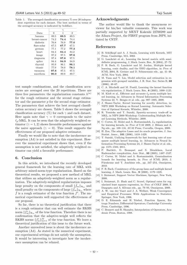
JSIAM Letters Vol. 5 (2013) pp.49–52 Taiji Suzuki
Table 1. The averaged classification accuracy % over 20 indepen-dent repetition for each dataset. The best method in terms of
the averaged accuracy is indicated by boldface.
γ
Data 0 1 2
banana 89.5 89.5 89.5breast-cancer 74.2 74.4 74.4
diabetis 76.8 76.9 77.0flare-solar 67.5 67.7 67.5
german 77.1 77.2 77.3heart 84.4 84.4 84.2image 97.2 97.5 97.6
ringnorm 97.4 97.6 97.5splice 94.4 94.9 94.9thyroid 95.9 96.1 96.1titanic 77.9 78.0 78.1
twonorm 97.6 97.5 97.5waveform 90.0 89.9 89.7
test sample combinations, and the classification accu-racies are averaged over the 20 repetitions. There arethree free parameters: the regularization constants λ(n)
for the rough estimator and the second stage estima-tor and the parameter p for the second stage estimator.The parameters that achieve the best averaged classifi-cation accuracy are chosen. Table 5 shows the averagedclassification accuracy (%) for each γ and each dataset.Here again note that γ = 0 corresponds to the naiveℓp-MKL. It can be seen that the adaptively weighted es-timator (γ = 1, 2) shows favorable performances againstthe naive approach (γ = 0). This result supports theeffectiveness of our proposed adaptive estimator.Finally we would like to note that the incoherence as-
sumption (A4) is not satisfied in this experiment. How-ever the numerical experiment shows that, even if theassumption is not satisfied, the adaptively weighted es-timator can yield a favorable performance.
6. Conclusion
In this article, we introduced the recently developedgeneral framework for the learning rate of MKL witharbitrary mixed-norm-type regularization. Based on thetheoretical results, we proposed a new method of MKLthat utilizes an adaptively-weighted norm as a regular-ization. The adaptively-weighted regularization imposeslarge penalty on the components of small ∥fm∥Hm andsmall penalty on the components of large ∥fm∥Hm wheref is a rough estimator of the true function f∗. The nu-merical experiments well supported the effectiveness ofour proposal.So far, there is no theoretical justification that there
is a rough estimator that can well estimate the RKHSnorm ∥f∗m∥Hm of the true function. Therefore there is noconfirmation that the adaptive-weight well reflects theRKHS norms f∗mMm=1 of the true function. We leave atheoretical justification of this issue to the future work.Another unresolved issue is about the incoherence as-
sumption (A4). As stated in the numerical experiment,our experimental settings do not satisfy the assumption.It would be interesting to investigate how the incoher-ence assumption can be relaxed.
Acknowledgments
The author would like to thank the anonymous re-viewer for his/her valuable comments. This work waspartially supported by MEXT Kakenhi 22700289 andthe Aihara Project, the FIRST program from JSPS, ini-tiated by CSTP.
References
[1] B. Scholkopf and A. J. Smola, Learning with Kernels, MIT
Press, Cambridge, MA, 2002.[2] G. Lanckriet et al., Learning the kernel matrix with semi-
definite programming, J. Mach. Learn. Res., 5 (2004), 27–72.[3] F. R. Bach, G. Lanckriet and M. Jordan, Multiple kernel
learning, conic duality, and the SMO algorithm, in: Proc ofICML 2004, R. Greiner and D. Schuurmans eds., pp. 41–48,ACM, New York, 2004.
[4] M. Yuan and Y. Lin, Model selection and estimation in re-
gression with grouped variables, J. R. Stat. Soc. Series B, 68(2006), 49–67.
[5] C. A. Micchelli and M. Pontil, Learning the kernel function
via regularization, J. Mach. Learn. Res., 6 (2005), 1099–1125.[6] M. Kloft et al., Efficient and accurate ℓp-norm multiple ker-
nel learning, in: Advances in Neural Information ProcessingSystems 22, Y. Bengio et al. eds., pp. 997–1005, 2009.
[7] J. Shawe-Taylor, Kernel learning for novelty detection, in:NIPS 2008 Workshop on Kernel Learning: Automatic Selec-tion of Optimal Kernels, Whistler, 2008.
[8] R. Tomioka and T. Suzuki, Sparsity-accuracy trade-off in
MKL, in NIPS 2009 Workshop: Understanding Multiple Ker-nel Learning Methods, Whistler, 2009.
[9] C. Cortes, M. Mohri and A. Rostamizadeh, L2 regularizationfor learning kernels, in: Proc of UAI 2009, J. Bilmes and A.
Ng eds., pp. 109–116, AUAI Press, Corvallis, Oregon, 2009.[10] H. Zou, The adaptive Lasso and its oracle properties, J. Am.
Statist. Assoc., 101 (2006), 1418–1429.
[11] T. Suzuki, Unifying framework for fast learning rate of non-sparse multiple kernel learning, in: Advances in Neural In-formation Processing Systems 24, J. Shawe-Taylor et al. eds.,pp. 1575–1583, 2011.
[12] P. Bartlett, O. Bousquet and S. Mendelson, LocalRademacher complexities, Ann. Stat., 33 (2005), 1487–1537.
[13] C. Cortes, M. Mohri and A. Rostamizadeh, Generalizationbounds for learning kernels, in: Proc of ICML 2010, J.
Furnkranz and T. Joachims eds., pp. 247–254, Omnipress,2010.
[14] F. R.Bach, Consistency of the group lasso and multiple kernellearning, J. Mach. Learn. Res., 9 (2008), 1179–1225.
[15] I. Steinwart, Support Vector Machines, Springer, New York,2008.
[16] I. Steinwart, D. Hush and C. Scovel, Optimal rates for reg-ularized least squares regression, in: Proc of COLT 2009, S.
Dasgupta and A. Klivans eds., pp. 79–93, Omnipress, 2009.[17] A. W. van der Vaart and J. A. Wellner, Weak Convergence
and Empirical Processes: With Applications to Statistics,
Springer, New York, 1996.[18] D. E. Edmunds and H. Triebel, Function Spaces, En-
tropy Numbers, Differential Operators, Cambridge UniversityPress, Cambridge, 1996.
[19] C. Bennett and R. Sharpley, Interpolation of Operators, Aca-demic Press, Boston, 1988.
– 52 –

JSIAM Letters Vol.5 (2013) pp.53–56 c⃝2013 Japan Society for Industrial and Applied Mathematics J S I A MLetters
The best estimation corresponding to
continuous model of Thomson cable
Hiroyuki Yamagishi1, Yoshinori Kametaka2, Atsushi Nagai3, Kohtaro Watanabe4
and Kazuo Takemura3
1 Tokyo Metropolitan College of Industrial Technology, 1-10-40 Higashi-ooi, Shinagawa, Tokyo140-0011, Japan
2 Osaka University, 1-3 Machikaneyama-cho, Toyonaka 560-8531, Japan3 Nihon University, 2-11-1 Shinei, Narashino 275-8576, Japan4 National Defense Academy, 1-10-20 Yokosuka 239-8686, Japan
E-mail yamagisi s.metro-cit.ac.jp
Received March 20, 2013, Accepted June 10, 2013
Abstract
We treat a continuous model of Thomson cable. The supremum of the absolute value of outputvoltage is estimated by the constant multiple of L2 norm of input voltage. We obtain the bestconstants of the above estimations, which are expressed as rational functions of resistance,capacitance and conductance constants. In the background, we have an initial boundary valueproblem of heat equation.
Keywords Thomson cable, heat kernel, modified Bessel function
Research Activity Group Applied Integrable Systems
1. Preperation
We treat transmission and earthed lines as Fig. 1. Re-sistance r is uniformly distributed in the transmissionline. Capacitance c and conductance g are uniformly dis-tributed between the transmission line and the earthedline. r, c, g are nonnegative constants and not all of themare zero. This is a continous model of Thomson cable dis-cussed in [1, 2]. u(x, t) is a voltage in the transmissionline at position x and time t. The initial voltage is 0,that is, u(x, 0) = 0. v(x, t) is an electric current in thetransmission line.From Ohm’s law and Kirchhoff’s law, we have
u(0, t)− u(x, t) =∫ x
0
r v(ξ, t)dξ,
v(0, t)− v(x, t) =∫ x
0
(c∂t + g)u(ξ, t)dξ.
Differentiating the above relation with respect to x, wehave
−∂xu(x, t) = rv(x, t),−∂xv(x, t) = (c∂t + g)u(x, t).
From this relation, we have (rc∂t − ∂2x + rg
)u = 0,
v(x, t) = −r−1∂xu(x, t).
In this paper, we give two inequalities on 0 < x < ∞and 0 < x < 1. In the case 0 < x < ∞, the supremumof |u(x, t)|2 is estimated by the constant multiple of thesquare of the L2 norm of input voltage given by
∥u(0, ·)∥2 =
∫ ∞
0
|u(0, t)|2dt.
cc
cc
0 x
u(0, t) u(x, t), v(x, t)
r
c, g
transmission line
earthed line
Fig. 1. Continous model of Thomson cable.
Simlilarly in the case 0 < x < 1, the supremumof |u(1, t)|2 is estimated by the constant multiple of∥u(0, ·)∥2. We obtain the best constants of the aboveestimations. The best constants are rational function ofthe constants r, c, g.In [1, 2], we consider the best estimation of Heaviside
cable and Thomson cable. In this paper, we consider thecontinuous version of the above results.
2. Thomson cable on a half line
In this section, we consider the case in which the trans-mission and earthed lines are half lines as Fig. 2. For anyfixed x ∈ (0,∞), we estimate the output voltage u(x, t)by the constant multiple of the power of input voltageu(0, t). We obtain the best estimation. For any fixed timet ∈ (0,∞), the input voltage u(x, t) is bounded functionwith respect to x ∈ (0,∞).Before stating the conclusion, we introduce a heat ker-
nel defined by
H(x, t) =1√4πt
e−x2
4t (0 < x <∞, 0 < t <∞).
Theorem 1 For any input voltage u(0, t) ∈ L2(0,∞)and arbitrarily chosen x ∈ (0,∞), the output voltage
– 53 –
JSIAM Letters Vol. 5 (2013) pp.53–56 Hiroyuki Yamagishi et al.
cc
cc
0 x
u(0, t) u(x, t), v(x, t)
r
c, g
Fig. 2. Continous model of Thomson cable in 0 < x < ∞.
u(x, t) satisfies the inequality(sup
0≤s<∞|u(x, s)|
)2
≤ C∥u(0, ·)∥2.
Among such C, the best constant is
C0 =
2
π
g
cK2(2
√rgx) (g > 0),
1
πrcx2(g = 0),
where Kn(z) is n-th kind modified Bessel function [3,p.170].
In the background of this theorem, we have the fol-lowing initial boundary value problem. Concerning theuniqueness and existence of the solution to the initialboundary value problem, we have the following lemma.
Lemma 2 For an arbitrary bounded continuous func-tion f(t) (0 < t <∞), the initial boundary value problem
IBVP(rc∂t − ∂2x + rg
)u = 0 (0 < x <∞, 0 < t <∞),
u(x, 0) = 0 (0 < x <∞),u(0, t) = f(t) (0 < t <∞),|u(x, t)| <∞ (0 < x <∞, 0 < t <∞)
has a unique solution as
u(x, t) =
∫ t
0
G(x, t− s)f(s)ds
(0 < x <∞, 0 < t <∞), (1)
where G(x, t) is given by
G(x, t) =x
te−
gtc H
(x,
t
rc
)(0 < x <∞, 0 < t <∞). (2)
Proof Through the transform
u(x, t)∣∣∣t=rcτ
= e−rgτw(x, τ)
(0 < x <∞, 0 < τ <∞), (3)
w(x, τ) satisfies the following equation:
IBVP(τ)(∂τ − ∂2x
)w = 0 (0 < x <∞, 0 < τ <∞),
w(x, 0) = 0 (0 < x <∞),w(0, τ) = g(τ) = ergτf(rcτ) (0 < τ <∞),| ecgτw(x, τ) | <∞ (0 < x <∞, 0 < τ <∞).
Through Laplace transform of w(x, τ) as
w(x, τ) −→ w(x, σ) =
∫ ∞
0
e−στw(x, τ)dτ,
for any fixed σ ∈ (0,∞), IBVP is converted to the fol-lowing equation:
IBVP˜[−(d/dx)2 + σ
]w = 0 (0 < x <∞),
w(0, σ) = g(σ),|w(x, σ)| <∞ (0 < x <∞).
The solution w(x, σ) to IBVP˜ is given as
w(x, σ) = e−√σxg(σ) (0 < x <∞). (4)
Applying the relation
|x|τH(x, τ) −→ e−
√σ|x| (5)
to (4), we have the solution to IBVP(τ) given as
w(x, τ) =
∫ τ
0
x
τ − τ ′H(x, τ − τ ′)g(τ ′)dτ ′
(0 < x <∞, 0 < τ <∞).
From (3), we have (1) and (2). Thus we prove Lemma 2.(QED)
Concerning L2 norm of G(x, t) with respect to t, wehave the following lemma.
Lemma 3 The relation ∥G(x, ·)∥2 = C0, which is de-fined in Theorem 1, holds.
Proof For any chosen x ∈ (0,∞), from (2), we have
∥G(x, ·)∥2
=
∫ ∞
0
|G(x, t)|2dt =∫ ∞
0
x2
t2e−
2gtc H2
(x,
t
rc
)dt
=rcx2
4π
∫ ∞
0
e−2gtc e−
2rcx2
4t t−3dt. (6)
Applying the formula of Laplace transform [4, p.291],∫ ∞
0
e−pte−a2
4t t−(ν+1)dt
=2ν+1p
ν2
aνKν(a
√p) (p, a > 0,−∞ < ν <∞), (7)
to (6), we have
∥G(x, ·)∥2 =2
π
g
cK2(2
√rgx).
If we set z = 2√rgx, then we have
∥G(x, ·)∥2 =2
πrcx2
(z2
)2K2(z).
Taking the limit as g → 0, that is, z → 0, we have
∥G(x, ·)∥2 =1
πrcx2,
where we have used the relation,(z2
)nKn(z) −−−→
z→0
1
2(n− 1)! (n = 1, 2, . . . ). (8)
This completes the proof of Lemma 3.(QED)
– 54 –

JSIAM Letters Vol. 5 (2013) pp.53–56 Hiroyuki Yamagishi et al.
3. Thomson cable on an interval
In this section, we consider the case in which the trans-mission and earthed lines are finite intervals as Fig. 3.We assume 0 < x < 1 without loss of generality. Weestimate the output voltage u(1, t) by the constant mul-tiple of the power of input voltage u(0, t). We imposea boundary condition v(1, t) = 0, which stands for anopen end. The next theorem states the best constant ofthis estimate.
Theorem 4 For any input voltage u(0, t) ∈ L2(0,∞),the output voltage u(1, t) satisfies the inequality(
sup0≤s<∞
|u(1, s) |)2
≤ C∥u(0, ·)∥2.
Among such C, the best constant is
C0 =
16
π
g
c
∞∑i,j=0
(−1)i+j(2i+ 1)(2j + 1)
(2i+ 1)2 + (2j + 1)2
×K2
(√2rg [(2i+ 1)2 + (2j + 1)2]
)(g > 0),
16
π
1
rc
∞∑i,j=0
(−1)i+j(2i+ 1)(2j + 1)
[(2i+ 1)2 + (2j + 1)2]2 (g = 0).
In the background of this theorem, we have the fol-lowing initial boundary value problem. Concerning theuniqueness and existence of the solution to the initialboundary value problem, we have the following lemma.
Lemma 5 For arbitrary bounded continuous functionf(t) (0 < t <∞), the initial boundary value problem
IBVP(rc∂t + rg − ∂2x
)u = 0 (0 < x < 1, 0 < t <∞),
u(x, 0) = 0 (0 < x < 1),u(0, t) = f(t) (0 < t <∞),∂xu(x, t)|x=1 = −rv(1, t) = 0 (0 < t <∞)
has a unique solution
u(x, t)=
∫ t
0
G(x, t−s)f(s)ds (0<x<1, 0<t<∞), (9)
where G(x, t) is given by
G(x, t)
= e−gtc
∞∑j=0
(−1)j
t
×[(x+2j)H
(x+2j,
t
rc
)+(1−x+2j+1)H
(1−x+2j+1,
t
rc
)].
(10)
Proof Through the same transformation as (3),w(x, τ) satisfies the following equation:
IBVP(τ)(∂τ − ∂2x
)w = 0 (0 < x < 1, 0 < τ <∞),
w(x, 0) = 0 (0 < x <∞),w(0, τ) = g(τ) = ergτf(rcτ) (0 < τ <∞),∂xw(x, τ)|x=1 = 0 (0 < τ <∞).
cc
cc
0 1
u(0, t) u(x, t), v(x, t)u(1, t)
v(1, t) = 0
r
c, g
Fig. 3. Continous model of Thomson cable in 0 < x < 1.
Through Laplace transform of w(x, τ), for any fixed σ ∈(0,∞), IBVP is converted to the following equation:
IBVP˜ [−(d/dx)2 + σ
]w = 0 (0 < x <∞),
w(0, σ) = g(σ), ∂xw(x, σ)|x=1 = 0.
The solution w(x, σ) to IBVP˜ is given as
w(x, σ)=cosh (
√σ(1− x))
cosh (√σ)
g(σ)
=
∞∑j=0
(−1)j(e−
√σ(x+2j)+e−
√σ(1−x+2j+1)
)g(σ).
Note that (5), we have the solution to IBVP(τ) as
w(x, τ)
=
∫ τ
0
∞∑j=0
(−1)j
τ − τ ′
× (x+2j)H(x+2j, τ−τ ′)+ [(1−x+2j+1)
×H(1−x+2j+1, τ − τ ′) ]g(τ ′)dτ ′
(0 < x <∞, 0 < τ <∞).
From (3), we have (9) and (10). Thus we prove Lemma 5.(QED)
Putting x = 1 in (9), we have
u(1, t) =
∫ t
0
G(1, t− s)f(s)ds (0 < t <∞), (11)
where
G(1, t) =2
te−
gtc
∞∑j=0
(−1)j(2j + 1)H
(2j + 1,
t
rc
)(0 < t <∞). (12)
Concerning L2 norm of G(1, t), we have the followinglemma.
Lemma 6 The relation ∥G(1, ·)∥2 = C0, which is de-fined in Theorem 4, holds.
Proof From (12), we have
∥G(1, ·)∥2 =
∫ ∞
0
|G(1, t)|2dt
=
∫ ∞
0
4
t2e−
2gtc
∞∑i,j=0
(−1)i+j(2i+ 1)(2j + 1)
×H(2i+ 1,
t
rc
)H
(2j + 1,
t
rc
)dt
– 55 –
JSIAM Letters Vol. 5 (2013) pp.53–56 Hiroyuki Yamagishi et al.
=rc
π
∞∑i,j=0
(−1)i+j(2i+ 1)(2j + 1)
×∫ ∞
0
t−3e−2gtc e−
rc4t [(2i+1)2+(2j+1)2]dt.
Applying (7) to the above relation, we have
∥G(1, ·)∥2
=16g
πc
∞∑i,j=0
(−1)i+j(2i+ 1)(2j + 1)
(2i+ 1)2 + (2j + 1)2
×K2
(√2rg [(2i+ 1)2 + (2j + 1)2]
).
If we set z =√2rg [(2i+ 1)2 + (2j + 1)2], then we have
∥G(1, ·)∥2
=16
πc
2
r
∞∑i,j=0
(−1)i+j(2i+ 1)(2j + 1)
[(2i+ 1)2 + (2j + 1)2]2
(z2
)2K2(z).
Taking the limit as g → 0, that is, z → 0, we have
∥G(1, ·) ∥2 =16
πrc
∞∑i,j=0
(−1)i+j(2i+ 1)(2j + 1)
[(2i+ 1)2 + (2j + 1)2]2 ,
where we have used (8). This completes the proof ofLemma 6.
(QED)
4. Proof of Theorems 1 and 4
In this section, we give a proof of main theorems.Proof of Theorem 1 For any chosen x ∈ (0,∞), weput
u(t) = u(x, t), f(t) = u(0, t), G(t) = G(x, t), (13)
for the sake of simplicity. Exchanging t and s in (1) andapplying Schwarz inequality, we have
|u(s)|2 ≤∫ s
0
|G(s− t)|2dt∫ s
0
|f(t)|2dt
=
∫ s
0
|G(t)|2dt∫ s
0
|f(t)|2dt.
Taking the supremum with respect to s, we obtain theinequality (
sup0≤s<∞
|u(s)|)2
≤ ∥G∥2∥f∥2. (14)
For the input voltage
F (t) = Y (t0 − t)G(t0 − t),
we set the output voltage
U(t) =
∫ t∧t0
0
G(t− s)G(t0 − s)ds (0 < t <∞),
where Y (t) is Heaviside step function Y (t) = 1 (0 ≤ t <∞), 0 (−∞ < t < 0) and t ∧ t0 = mint, t0. We notethat
U(t0)=
∫ t0
0
|G(s)|2ds, ∥F∥2=∫ t0
0
|G(s)|2ds = U(t0).
Putting u(t) = U(t) in (14), we have(sup
0≤s<∞|U(s)|
)2
≤ ∥G∥2∥F∥2 = ∥G∥2U(t0).
Together with a trivial inequality
(U(t0))2 ≤
(sup
0≤s<∞|U(s)|
)2
,
we have
(U(t0))2 ≤
(sup
0≤s<∞|U(s)|
)2
≤ ∥G∥2U(t0).
Dividing this inequality by ∥F∥2 = U(t0) > 0, we have
U(t0) ≤
(sup
0≤s<∞|U(s)|
)2
∥F∥2≤ ∥G∥2.
Taking the limit t0 →∞ and considering that
U(t0) −→ ∥G∥2,
we have Theorem 1.(QED)
It should be noted that Theorem 4 is proved in thesame way by putting u(t) = u(1, t), G(t) = G(1, t) in(13).
References
[1] Y. Kametaka, K. Takemura, H. Yamagishi, A. Nagai and K.
Watanabe, Heaviside cable, Thomson cable and the best con-stant of a Sobolev-type inequality, Sci. Math. Jpn., e-2007(2007), 739–755.
[2] K. Takemura, Y. Kametaka, K. Watanabe, A. Nagai and
H. Yamagishi, Sobolev type inequalities of time-periodicboundary value problems for Heaviside and Thomson cables,Bound. Value Probl., 2012:95 (2012).
[3] S.Moriguchi, K.Udagawa and S.Hitotsumatsu, Iwanami Sug-
aku Koshiki III (in Japanese), Iwanami, Tokyo, 1960.[4] S.Moriguchi, K.Udagawa and S.Hitotsumatsu, Iwanami Sug-
aku Koshiki II (in Japanese), Iwanami, Tokyo, 1960.
– 56 –
JSIAM Letters Vol.5 (2013) pp.57–60 c⃝2013 Japan Society for Industrial and Applied Mathematics J S I A MLetters
A new method for fast computation of cumulative
distribution functions by fractional FFT
Ken’ichiro Tanaka1
1 School of Systems Information Science, Future University Hakodate, 116-2 Kamedanakano-cho, Hakodate, Hokkaido 041-8655, Japan
E-mail ketanaka fun.ac.jp
Received February 21, 2013, Accepted June 12, 2013
Abstract
We consider computation of cumulative distribution functions from their corresponding char-acteristic functions. We may use some known formulas with singular integrals for the compu-tation. It is, however, difficult to speed up the computation with such formulas, because thefast Fourier transform (FFT) cannot be applied directly to them. Based on existing works forpricing of financial derivatives, we propose a fast method for the computation with fractionalFFT and obtain accurate results on the entire real line.
Keywords cumulative distribution function, characteristic function, fractional FFT
Research Activity Group Scientific Computation and Numerical Analysis
1. Introduction
In this paper, we propose a fast method for computingcumulative distribution functions from their correspond-ing characteristic functions. Such computation is oftenneeded in fields where stochastic modeling is employedsuch as physics, statistics, and finance, etc. In the fieldof finance, pricing of financial derivatives is one of majorpurposes, for which stochastic processes Xt are used tomodel asset prices related to the financial derivatives.For the pricing problem, it is fundamental to compute
the distribution functions F (x) = P (Xt ≤ x). For somepopular stochastic processes Xt often employed for themodeling, the characteristic functions ϕ of Xt can beobtained analytically, whereas the closed forms of thecorresponding distribution functions F are not available[1]. Even in such cases, F can be numerically computedfrom ϕ by an inversion formula with the Fourier trans-form. For such computation, we may use some funda-mental formulas with singular integrals [2]. It is, how-ever, difficult to speed up the computation, because thefast Fourier transform (FFT) cannot be applied directlyto them due to the singularity of the integrals.Carr and Madan [3] pioneered in fast computation
for derivative pricing using the FFT. Their methodshave been used and developed by many authors (see [1]and the references therein). In particular, Chourdakis[4] improved efficiency of the computation using frac-tional FFT, which allows arbitrary width of equispasedgrids for discretization of the Fourier transform. Carrand Madan’s methods and Chourdakis’s improvementcan be applied to the computation of F from ϕ. Re-cently, Nakajima [5] proposed a method for the compu-tation based on their works. His method is effective, butproduces error not negligible for F (x) at large |x|. Then,we propose a method to overcome this problem.The rest of this paper is organized as follows. In Sec-
tion 2, mathematical formulation of our problem is pre-sented. In Section 3, we review some existing works withnumerical examples. Our method is proposed and nu-merical examples for it are shown in Sections 4 and 5,respectively. Section 6 concludes.
2. Mathematical preliminaries
In the rest of this paper, we consider a one dimen-sional random variable X, dropping the subscript t. Letf be the probability density function of X, let F bethe cumulative distribution function of X and let ϕ bethe characteristic function of X. Note that the followingfundamental relations among them:
F (x) =
∫ x
−∞f(t) dt, (1)
ϕ(u) = E[eiuX
]=
∫ ∞
−∞f(x) eiux dx. (2)
Furthermore, when ϕ is given, f can be obtained by
f(x) =1
2π
∫ ∞
−∞ϕ(u) e−iux du, (3)
i.e., the inverse Fourier transform of ϕ.Applying some standard numerical integration for-
mula to (3) and (1), we can compute f(x) and F (x).More precisely, for x = xn with n = −N, . . . , N − 1, wecan use a formula for (3) such as
f(xn) ≈1
2π
M−1∑m=−M
wmϕ(um)e−iumxn , (4)
where wmM−1m=−M and umM−1
m=−M are some finite se-quences. Furthermore, we can use the values f(xn) (n =−N, . . . , N − 1) to approximate F (xn) in (1) similarlyto (4). Then, in a naive manner, computational cost ofF (x) for a fixed x = xn is O(MN).
– 57 –

JSIAM Letters Vol. 5 (2013) pp.57–60 Ken’ichiro Tanaka
In practice, however, it is desirable to obtain the val-ues of F (xn) (n = −N, . . . , N − 1) as fast as possible. Apromising steps to achieve effective computation are:
1. deriving F directly from ϕ with the inverse Fouriertransform, and
2. computing the transform with the FFT.
The difficulty in the step 1 is that F does not have theusual Fourier transform onR because limx→∞ F (x) = 1.This can be remedied in some ways. For example, thereis a known fundamental formula [2]
F (x) =1
2− 1
2π
∫ ∞
−∞
ϕ(u)
iue−ixu du. (5)
In this paper, some simple deformations Fρ of F aretreated such that they have closed forms of the Fouriertransform ψρ expressed by ϕ. These are described in Sec-tions 3 and 4. The step 2 is computation of the sums:
Fρ(xn) ≈1
2π
M−1∑m=−M
wmψρ(um)e−iumxn (6)
for n = −N, . . . , N − 1, which requires equispaced gridsumM−1
m=−M and xnN−1n=−N such that M = N and
umxn =πmn
N(7)
in order to apply the FFT directly to (6). This require-ment can be relaxed by fractional FFT, as described inSections 3. Note that, if these two steps are realized, thecomputational cost of F (xn) (n = −N, . . . , N−1) in thecase M = N is O(N logN).
3. Existing works
In this section, we review some existing works relatedto computation of distribution functions F , and specifythe motivation of our work.
3.1 Nakajima’s idea based on Carr and Madan’s meth-od and fractional FFT
Carr and Madan [3] introduced effective methods forderivative pricing using the FFT. Derivative prices canbe mathematically described as expectations of somefunctions of random variables describing some finan-cial markets. The probability distributions of the ran-dom variables are determined by some stochastic mod-els. Since some popular models can give closed forms ofthe characteristic functions of the random variables [1],Carr and Madan developed a simple analytic expres-sion for the Fourier transform of the derivative price,and used the FFT to numerically compute it. Moreover,Chourdakis [4] used fractional FFT, which is describedin Section 3.2, for the computation of the Fourier trans-form to relax the requirement of equispaced grids suchas (7) in Carr and Madan’s method, and improved effi-ciency of the computation.Recently, Nakajima [5] proposed a method to com-
pute distribution functions based on Carr and Madan’smethod and fractional FFT. According to Carr andMadan’s idea, Nakajima considered a function Fρ de-fined by Fρ(x) = e−ρxF (x) for some ρ > 0, which cor-responds to the step 1 in Section 2. Then, if F decays
exponentially as x → −∞ and ρ is not so large, thefunction Fρ has the Fourier transform
ψρ(u) =
∫ ∞
−∞Fρ(x)e
iuxdx (8)
with explicit form
ψρ(u) =ϕ(u+ ρi)i
u+ ρi. (9)
Therefore it follows that
F (x) =eρx
2π
∫ ∞
−∞ψρ(u)e
−iuxdu. (10)
Then, application of the trapezoidal formula to theintegral in (10) yields
F (nh) ≈ eρnh
2πGψρ,h,N (nh) (11)
where h, h > 0 and
Gψρ,h,N (x) =N−1∑m=−N
hψρ(mh)e−imhx. (12)
These correspond to (6) in the step 2 in Section 2, wherewm = h, um = mh and xn = nh, i.e., h and h are thewidth of the grids um and xn, respectively. In orderto use the FFT directly for the computation of (12), hand h need to satisfy
hh =π
N(13)
due to (7). Then, in order to obtain accurate approxi-mations of F (nh) (n = −N, . . . , N − 1), we need to usesmall h, which requires large h. This means that accuratecomputation with the FFT is possible only for a sparsegrid nh. According to Chourdakis [4], Nakajima re-laxed the requirement (13) by applying fractional FFTto (12).
3.2 Fractional FFTFractional FFT is developed by Bailey and Swarz-
trauber [6] to enable computation of the discrete Fouriertransforms such as (12) with arbitrary h and h. The frac-tional FFT is derived by regarding the sum in (12) as acircular convolution. Noting 2mn = m2+n2− (m−n)2,for n = −N, . . . , N − 1 we have
Gψρ,h,N (nh) =N−1∑m=−N
hψρ(mh)e−πi[m2+n2−(m−n)2]α
= e−πin2α
N−1∑m=−N
ymzn−m, (14)
where α = hh/(2π), ym = hψρ(mh)e−πim2α and zm =
eπim2α. Since z−m = zm, it suffices to consider zm2Nm=0.
Note that the sum in (14) is a convolution but not circu-lar, i.e., we cannot regard zm2Nm=0 as 2N -periodic suchas zm+2N = zm. Then, we need to convert this sum intoa form of a circular convolution. A way for this conver-sion is to extend ymN−1
m=−N and zm2Nm=0 to length 4Nas follows:
ym = 0 (−2N ≤ m < −N,N ≤ m < 2N), (15)
– 58 –

JSIAM Letters Vol. 5 (2013) pp.57–60 Ken’ichiro Tanaka
zm = eπi(m−4N)2α (2N < m < 4N), (16)
and extend zm4N−1m=0 to 4N -periodic one for −4N ≤
m < 0. Then, we have the circular convolution
Gψρ,h,N (nh) = e−πin2α
2N−1∑m=−2N
ymzn−m. (17)
Finally, we can use the ordinal FFT to compute (17)with computational cost O(N logN).
3.3 Numerical examples
We show numerical examples for the method basedon (11) and the fractional FFT. We treat the standardnormal distribution N(0, 1) and the gamma distributionGa(2, 1). Their distribution functions FN and FGa, andcharacteristic functions ϕN and ϕGa are as follows:
FN(x) =1√2π
∫ x
−∞e−
t2
2 dt, ϕN(u) = e−u2
2 ,
FGa(x) =
0 (x < 0),
1− (1 + x)e−x (x ≥ 0),
ϕGa(u) = (1− iu)−2.
As for the parameters in (11), we set
N = 2048, h =5
N, h =
10
N, ρ = 0.9. (18)
That is, the interval on which ϕN and ϕGa are evaluatedis [−5, 5], and the interval on which FN and FGa are com-puted is [−10, 10]. Programs for these computations arewritten in C with double-precision floating-point arith-metic. The results are shown by Figs. 1 and 2. Theseresults show that the accuracy is relatively bad at largexn = nh, i.e., at the tails of the distributions.We can give theoretical explanation for these results.
The error of the approximation (11) is estimated as∣∣∣∣∣F (nh)− eρnh
2πGψρ,h,N (nh)
∣∣∣∣∣ = eρnh
2πEψρ,h,N (nh), (19)
where
Eψρ,h,N (nh) =∣∣∣2πFρ(nh)−Gψρ,h,N (nh)
∣∣∣ (20)
is the error of the trapezoidal formula. We can considertwo causes for the bad error as follows:
1. The error Eψρ,h,N (nh) in (20) may become large
when |nh| ≫ π/h, because Fρ(x) is not periodicwhereas Gψρ,h,N (x) in (12) has period 2π/h.
2. Even if Eψρ,h,N (nh) is sufficiently small for any n,
the increasing factor eρnh in (19) may make thetotal error worse for large n.
Then, we propose a method to remove these causes inSection 4.
4. Proposed method
In this section, we propose a method which enablesfast and accurate computation of distribution functionsF on the entire real line R. In the following, we writedown an algorithm and then show its validity.
1e-10
1e-9
1e-8
1e-7
1e-6
1e-5
1e-4
1e-3
1e-2
1e-1
1e0
-10 -5 0 5 10
Abso
lute
Err
or
x
N(0,1), rho = 0.90
Fig. 1. The error of the method based on (11) for the normaldistribution N(0, 1).
1e-10
1e-9
1e-8
1e-7
1e-6
1e-5
1e-4
1e-3
1e-2
1e-1
1e0
-10 -5 0 5 10
Abso
lute
Err
or
x
Ga(2,1), rho = 0.90
Fig. 2. The error of the method based on (11) for the gamma
distribution Ga(2, 1).
4.1 Proposed method
Suppose that the characteristic function ϕ is analyticon the region Dd defined by Dd = z ∈ C | Im |z| < dfor some d > 0. Then, our method is described as follows:
Step 1. For given ϕ, define ζ by
ζ(u) =
i
(ϕ(u)
u− π
2 sinh(πu2
)) (u = 0),
iϕ′(0) (u = 0).
(21)
Step 2. For ε with 0 < ε < mind, 1, choose ρ with0 < ρ ≤ mind, 1 − ε and define γ by
γ(u) =ζ(u− ρ i) + ζ(u+ ρi)
2. (22)
Step 3. Consider approximation of the inverse Fouriertransform of γ as
ΓN,h(nh) =1
2π
N−1∑m=−N
hγ(mh)e−imnhh, (23)
and apply the fractional FFT to computation of(23) for n = −N, . . . , N − 1.
Step 4. As approximations of the values F (nh) (n =−N, . . . , N − 1), compute(
cosh(ρnh))−1
ΓN,h(nh) +1
2
(tanh(nh) + 1
).
The analyticity of ϕ on Dd is necessary for the exis-tence of the inverse Fourier transform of γ. Note thatthe last step contains multiplication of the decay factorcosh(ρnh)−1 to ΓN,h(nh), which removes the causes1 and 2 of the bad errors at the tail of the distribu-tions pointed out in Section 3.3. Validity of the methodis shown in Section 4.2.
– 59 –

JSIAM Letters Vol. 5 (2013) pp.57–60 Ken’ichiro Tanaka
4.2 Validity of the proposed method
Validity of the proposed method follows from the fol-lowing two propositions. For the distribution functionF , set F (x) = F (x) − (tanhx+ 1) /2 and Fρ(x) =
cosh(ρx)F (x). Proof of Proposition 2 is straightforwardand then omitted.
Proposition 1 The Fourier transform of the functionF (x) exists and is written in the form (21).
Proposition 2 The Fourier transform of the functionFρ(x) exists and is written in the form (22).
Proof of Proposition 1 Set T (x) = (tanhx + 1)/2and let τ denote the Fourier transform of T ′(x). Then itfollows that
τ(u) =πu
2 sinh(πu2
) . (24)
Let H be the Heaviside function
H(x) =
1 (x ≥ 0),
0 (x < 0),
and set Z(x) = F (x)−H(x) and W (x) = T (x)−H(x).Then, Z and W have the Fourier transforms η and θ,respectively, which are written in the forms
η(u) =1− ϕ(u)
iu, θ(u) =
1− τ(u)iu
. (25)
Therefore, the Fourier transform of F (x) = F (x) −T (x) = Z(x)−W (x) coincides with
η(u)− θ(u) = iϕ(u)− τ(u)
u(26)
for u = 0. Thus we obtain (21).(QED)
5. Numerical examples
Using the proposed method, we treat again the nor-mal distribution N(0, 1) and the Gamma distributionGa(2, 1). We used the same parameters as (18). Theresults are shown by Figs. 3 and 4, respectively. Fromthese results, we can expect that the proposed methodenables accurate computation of distribution functionson the entire real line.Theoretical support for these results is given in a sim-
ilar manner to (19) and (20). The total error of the pro-posed method is(
cosh(ρnh))−1 ∣∣∣cosh(ρnh)F (nh)− ΓN,h(nh)∣∣∣ . (27)
This is a product of the decay factor (cosh(ρnh))−1
and the error of the trapezoidal formula for the in-verse Fourier transform. Therefore the total error is sup-pressed even if |nh| is large. We emphasize that it is onthe entire real line that the proposed method achievesenough accuracy, although it produces worse error forsome x = nh than the existing method based on (11).
6. Concluding remarks
Using the fractional FFT, we have proposed a fastmethod for computing distribution functions F fromtheir corresponding characteristic functions ϕ which are
1e-10
1e-9
1e-8
1e-7
1e-6
1e-5
1e-4
1e-3
1e-2
1e-1
1e0
-10 -5 0 5 10
Abso
lute
Err
or
x
N(0,1), rho = 0.90
Fig. 3. The error of the proposed method for the normal distri-bution N(0, 1).
1e-10
1e-9
1e-8
1e-7
1e-6
1e-5
1e-4
1e-3
1e-2
1e-1
1e0
-10 -5 0 5 10
Abso
lute
Err
or
x
Ga(2,1), rho = 0.90
Fig. 4. The error of the proposed method for the gamma distri-
bution Ga(2, 1).
analytic on the region Dd. Our method enables accuratecomputation on the entire real line, which is supportedby the numerical examples and the theoretical estimate.As future works, we may consider optimal error con-
trol based on rigorous error analysis of our method, ac-celerating convergence of the method, or modification ofthe method for ϕ with weaker analyticity, and so on.
Acknowledgments
The author gives special thanks to Prof. Masaaki Sug-ihara for his variable comments about this work. Thiswork is supported by JSPS KAKENHI Grant Number24760064.
References
[1] Y.K.Kwok, K.S.Leung and H.Y.Wong, Efficient options pric-ing using the fast Fourier transform, in: Handbook of Compu-
tational Finance, J.-C. Duan et al. eds., pp. 579–604, Springer-Verlag, Berlin, 2012.
[2] L.A.Waller, B.W.Turnbull and J.M.Hardin, Obtaining distri-
bution functions by numerical inversion of characteristic func-tions with applications, Amer. Statist., 49 (1995), 346–350.
[3] P. Carr and D. B. Madan, Option valuation using the fastFourier transform, J. Comput. Finance, 2 (1999), 61–73.
[4] K. Chourdakis, Option pricing using the fractional FFT, J.Comput. Finance, 8 (2005), 1–18.
[5] R. Nakajima, Valuation of credit default swaps with counterparty risks (in Japanese), Master’s Thesis, The Univ. of Tokyo,
2012.[6] D. H. Bailey and P. N. Swarztrauber, The fractional Fourier
transform and applications, SIAM Review, 33 (1991), 389–404.
– 60 –

JSIAM Letters Vol.5 (2013) pp.61–64 c⃝2013 Japan Society for Industrial and Applied Mathematics J S I A MLetters
Construction method of the cost function for the minimax
shape optimization problem
Kouhei Shintani1 and Hideyuki Azegami1
1 Nagoya University, A4-2 (780) Furo-cho, Chikusa-ku, Nagoya 464-8601, Japan
E-mail shintani az.cs.is.nagoya-u.ac.jp
Received April 1, 2013, Accepted June 7, 2013
Abstract
The present paper describes a method by which to formulate a shape optimization problem of alinear elastic continuum for minimizing the maximum value of a strength measure, such as thevon Mises stress. In order to avoid the irregularity of the shape derivative of the maximumvalue, the Kreisselmeier–Steinhauser function of the strength measure is used as the costfunction. In the cost function, a parameter is used to control the regularity of the shapederivative. In the present paper, we propose a rule by which to appropriately determine theparameter. The effectiveness of the proposed rule is confirmed through a numerical exampleof a cantilever problem.
Keywords calculus of variations, boundary value problem, shape optimization, H1 gradientmethod, Kreisselmeier-Steinhauser function
Research Activity Group Mathematical Design
1. Introduction
In the design of parts of machines or mechanical struc-tures, strength is one of the most important factors. Inpractice, the maximum von Mises stress is evaluated atall times and all locations for parts constructed fromductile metal, which is modeled as a linear elastic body,and is used as a measure of the strength. Hence, in orderto find the optimum shape of a linear elastic body whilemaximizing the strength, we must construct a shape op-timization problem involving the minimization of themaximum von Mises stress, which we refer to as the min-imax shape optimization problem. However, this prob-lem is irregular because we cannot define the Frechetderivative with respect to domain variation, which werefer to as the shape derivative, of the cost function,such as the maximum value of the von Mises stress.In order to avoid irregularity, the Kreisselmeier–
Steinhauser function [1], which is referred to hereinafteras the KS function, with respect to a strength measuresuch as the von Mises stress has been used instead ofthe maximum value of a strength measure. We can de-fine the shape derivative of the KS function and obtaina numerical solution by the finite element method, asshown in [2].However, in the KS function, a parameter p ∈ (0,∞)
is used to control the regularity of the shape deriva-tive of the KS function. When p → ∞, the value ofthe KS function approaches the maximum value of thestrength measure, while the regularity worsens simulta-neously. Actually, convergence phenomena are affectedby the value of p. An appropriate value of p has beendetermined empirically.In the present paper, we propose a rule by which to
determine the value of p. Using this rule, we construct
a shape optimization problem with the KS function asa cost function. The method for computing the shapederivative of the cost function is given as an adjoint vari-able method considering the rule for p. A solution to thisnew problem is presented based on the algorithm of se-quential quadratic programming using the H1 gradientmethod for reshaping in order to maintain the smooth-ness of the boundary [3–6]. The effectiveness of the rulefor p is confirmed based on a numerical solution to acantilever problem.
2. Admissible set of design variables
First, let us define the admissible set of design vari-able for the shape optimization problem. Let D0 andΩ0 ⊂ D0 be d ∈ 2, 3 dimensional domains with Lip-schitz boundaries, which are denoted by ∂D0 and ∂Ω0.On ∂Ω0, ΓD0 ⊂ ∂Ω0 and ΓN0 = ∂Ω0 \ ΓD0 (ΓD0 =ΓD0∪∂ΓD0) denote the Dirichlet boundary and the Neu-mann boundary, respectively. Moreover, let Γp0 ⊂ ΓN0
be a non-homogeneous Neumann boundary. We assumethatD0 and Ω0 are fixed and that mapping ϕ : D0 → Rdincluded in a Banach of
Y =W 1,∞ (D0;Rd)
(1)
is a design variable in the shape optimization problem.Moreover, we let
D =ϕ ∈ Y
∣∣ ∥ϕ− ϕ0∥W 1,∞(D0;Rd) < 1,ϕ (Ω0) ⊆ D0,
piecewise C2 class on Γp0,
ϕ = ϕ0 on ΓC0
(2)
be the admissible set of design variable ϕ, where ΓC0 ⊂∂Ω0 denotes a boundary on which domain variationis constrained due to design considerations. In (2),∥ϕ − ϕ0∥W 1,∞(D0;Rd) < 1 is used to assure one-to-one
– 61 –

JSIAM Letters Vol. 5 (2013) pp.61–64 Kouhei Shintani et al.
¡D0
¡p0
0
p0
b0
uD0
(Á)
Fig. 1. Initial domain Ω0 and variation domain Ω(ϕ).
mapping. In the present paper, we use the notationΩ(ϕ) for ϕ(x) |x ∈ Ω0 and ∂Ω−(ϕ) for the openset ∂Ω(ϕ) \ Θ(ϕ), where Θ(ϕ) denotes the set of cor-ner points of measure 0.
3. Main problem
Using the design variable ϕ ∈ D, let us define themain problem as a shape optimization problem. In thepresent paper, we consider a linear elastic problem asthe main problem. We have the following assumptions.
(H1) For q > d, b ∈ L2q(D0;Rd), p ∈ W 1,2q
(D0;Rd), uD ∈ W 1,2q(D0;Rd), and C ∈ W 1,∞
(D0;Rd×d×d×d) denote the volume force, the trac-tion force, and the given displacement and stiffness,respectively. For C, we assume that there exist pos-itive constants α and β such that X · (CX) ≥α∥X∥2, |X · (CY )| ≤ β∥X∥∥Y ∥ for all X,Y ∈X ∈ Rd×d |X =XT and Cijkl = Cklij at almostall of D0.
(H2) For ∂Ω(ϕ), opening angles at corner points Θ(ϕ)and the boundary of mixed boundary conditions∂ΓD(ϕ) are less than π and π/2, respectively (seeFig. 1).
Under the assumptions, we let
S =u ∈W 2,2q
(D0;Rd
)| ϕ ∈ D
(3)
be the admissible set for displacement u. Let T (u) =CE(u) and E(u) = [∇uT + (∇uT)T]/2 denote thestress and strain, respectively. Moreover, we use ν asthe outer unit normal on the boundary.
Problem 1 (Linear elastic problem) For ϕ ∈ D,let (H1) and (H2) be satisfied. Find u ∈ S such that
−∇TT (u) = bT in Ω(ϕ) ,
T (u)ν = p on Γ−p (ϕ) ,
T (u)ν = 0 on Γ−N (ϕ) \ Γp (ϕ) ,
u = uD on ΓD (ϕ) .
For use in Section 5, we here define the Lagrange func-tion for the main problem (Problem 1) as
LM (ϕ,u,v)
=
∫Ω(ϕ)
(−T (u) ·E (v)+b · v) dx+
∫ΓN(ϕ)
p · v dγ
+
∫Γ−D(ϕ)
[(u−uD) · T (v)ν+v · T (u)ν] dγ, (4)
where v ∈ S is introduced as the Lagrange multiplier.With LM(ϕ,u,v), if u is the solution of Problem 1, then
LM(ϕ,u,v) = 0
holds for all v ∈ S.
4. Shape optimization problem
Using the solution u of Problem 1 for ϕ ∈ D, we definethe cost functions as follows. In the present paper, we areattempting to construct a cost function for the strengthof a linear elastic body. Here, we let σ : Rd → R bea function of u representing a measure of strength. Inthe present paper, we use the von Mises stress for themeasure given by
σ (u) =
√3
2TD (u) · TD (u),
where TD(u) denotes the deviator stress, which is de-fined as
TD (u) = T (u)− 1
3tr (T (u)) I,
and I denotes the unit tensor.As a cost function of strength, we set the objective
function as follows:
f0 (ϕ,u, p) =1
pln
∫Ω(ϕ)
epσ(u)dx∫Ω(ϕ)
dx
. (5)
In (5), p ∈ (0,∞) is assumed to be a constant in theprevious papers [1,2]. However, in the present paper, weassume that
p =
∫Ω(ϕ)
dx∫Ω(ϕ)
σ (u) dx
− 1
c0(6)
holds, where c0 denotes a positive constant, which indi-cates maxx∈Ω0 σ(u(x)) with the solution u of Problem1 for Ω0. Moreover, p is considered to be the deviation ofthe inverse of the maximum value of the strength mea-sure from the inverse of the average value of the strengthmeasure. In this sense of p, the index pσ(u) in (6) refersto a normalized index for the deviation of the strengthmeasure.On the other hand, as a cost function that has a trade-
off relation with respect to f0, we define the followingconstraint function for the mass:
f1 (ϕ) =
∫Ω(ϕ)
ρdx− c1, (7)
where ρ ∈ W 1,∞(D0;R) is the density, and c1 is a pos-itive constant such that there exists some ϕ ∈ D thatsatisfies f1(ϕ) < 0.Using the cost functions, we construct the shape op-
timization problem as follows.
Problem 2 (Strength maximization problem)Let f0(ϕ,u, p) and f1(ϕ) be defined in (5) and (7),
– 62 –

JSIAM Letters Vol. 5 (2013) pp.61–64 Kouhei Shintani et al.
respectively. Find ϕ such that
minϕ∈D
f0 (ϕ,u, p) | f1 (ϕ) ≤ 0,
u ∈ S, Problem 1 and (6).
5. Shape derivative of the cost functions
Let φ ∈ Y be the domain variation from ϕ. We referto the Frechet derivatives of f0 and f1 with respect toarbitrary φ ∈ Y as the shape derivatives, and we denotethese derivatives as f ′0(ϕ,u, p)[φ,u
′, p′] and f ′1(ϕ)[φ],respectively, where u′ and p′ denote the variations of uand p, respectively, caused by φ that satisfy Problem 1and (6).The shape derivative of f1 is obtained using the for-
mula of the shape derivative for the domain integral [7]as
f ′1 (ϕ) [φ] = ⟨g1,φ⟩ =∫∂Ω(ϕ)
ρν ·φdγ. (8)
On the other hand, the shape derivative of f0 is ob-tained as follows. Let
L0 (ϕ,u,v0, p, q0)
= f0 (ϕ,u, p) + q0
p+ 1
c0−
∫Ω(ϕ)
dx∫Ω(ϕ)
σ (u) dx
+ LM (ϕ,u,v0)
be the Lagrangian for f0, where v0 ∈ S and q0 ∈ R areintroduced as Lagrange multipliers. The shape derivativeof L0(ϕ,u,v0, p, q0) is written as follows:
L ′0 (ϕ,u,v0,p,q0) [φ,u
′, p′]
= L0ϕ (ϕ,u,v0,p,q0) [φ] + L0u (ϕ,u,v0,p,q0) [u′]
+ L0v0 (ϕ,u,v0,p,q0) [v′0] + L0p (ϕ,u,v0,p,q0) [p
′]
+ L0q0 (ϕ,u,v0,p,q0) [q′0] . (9)
Here, if u is the solution to Problem 1 and p is deter-mined by (6), then the third and fifth terms in the right-hand side of (9) become 0.The fourth term in the right-hand side of (9) is calcu-
lated as
L0p (ϕ,u,v0, p, q0) [p′]
=
− 1
p2ln
∫Ω(ϕ)
epσ(u) dx∫Ω(ϕ)
dx
−
∫Ω(ϕ)
epσ(u)σ (u) dx
p
∫Ω(ϕ)
epσ(u) dx
+q0
p′.
Then, the fourth term becomes 0, if q0 is determined by
q0 =1
p2ln
∫Ω(ϕ)
epσ(u) dx∫Ω(ϕ)
dx
+
∫Ω(ϕ)
epσ(u)σ (u) dx
p
∫Ω(ϕ)
epσ(u) dx
. (10)
Moreover, the second term in the right-hand side of(9) is calculated as
L0u (ϕ,u,v0, p, q0) [u′]
=
∫Ω(ϕ)
epσ(u) ∂σ (u)
∂T (u)· T (u′) dx
p
∫Ω(ϕ)
epσ(u) dx
+ q0
∫Ω(ϕ)
dx
∫Ω(ϕ)
eσ(u) ∂σ (u)
∂T (u)· T (u′) dx(∫
Ω(ϕ)
σ (u) dx
)2
+ LM (ϕ,u′,v0)
=
∫Ω(ϕ)
Σ (u, p, q0) · T (u′) dx+ LM (ϕ,u′,v0) . (11)
Then, the second term becomes 0 if v0 is the solution tothe following adjoint problem.
Problem 3 (Adjoint problem for f0) Let u be thesolution to Problem 1, and let p and q0 be given by (6)and (10), respectively. Find v0 ∈ S such that
−∇TT (v0) = −∇TΣ (u, p, q0) in Ω(ϕ) ,
T (v0)ν = 0 on Γ−p (ϕ) ,
T (v0)ν = 0 on Γ−N (ϕ) \ Γp (ϕ) ,
v0 = 0 on ΓD (ϕ) ,
where Σ(u, p, q0) is defined in (11).
Considering the above conditions, if we use the so-lutions of u and v0 of Problem 1 and Problem 3, re-spectively, and p and q0 are determined by (6) and (10),respectively, then (9) becomes
L0ϕ (ϕ,u,v0, p, q0) [φ]
= f ′0 (ϕ,u, p) [φ]
=
∫∂Ω−(ϕ)
ζ∂Ων ·φdγ +
∫Γ−D(ϕ)
ζDν ·φdγ
+
∫Γ−N (ϕ)
(φ ·∇ζN + κζN)ν ·φdγ
+
∫∂ΓN(ϕ)∪Θ(ϕ)
ζNτ ·φdς = ⟨g0,φ⟩ (12)
where
ζ∂Ω =−1
p
∫Ω(ϕ)
dx
+epσ(u)
p
∫Ω(ϕ)
epσ(u)dx
+q0pσ (u)∫Ω(ϕ)
dx
−q0p
∫Ω(ϕ)
σ (u) dx(∫Ω(ϕ)
dx
)2
− T (u) ·E (v0) + b · (u+ v0)
ζD = T (u− uD) ·E (v0) + T (v0 − uD) ·E (u)
ζN = p · (u+ v0)
in which τ denotes the outer unit tangent of Γ−N(ϕ) for
d = 2 and the outer unit tangent of Γ−N(ϕ) and the outer
unit normal of ∂ΓN(ϕ)∪Θ(ϕ) for d = 3, and κ = ∇ · ν.
– 63 –

JSIAM Letters Vol. 5 (2013) pp.61–64 Kouhei Shintani et al.
¡D0
p
¡p00
x1 x2
x3
(a) Linear elastic problem (Problem 1)
¡C0
0
¡C0
(b) Domain variation
Fig. 2. Boundary conditions in the cantilever problem.
6. Solution
The algorithm for solving Problem 2 based on the se-quential quadratic programming is shown in previouspapers [5,6]. In this algorithm, the H1 gradient methodis used for reshaping with shape derivatives g0 and g1in (12) and (8), respectively.
7. Numerical example
We developed a program based on an algorithm usingthe finite element method. Using this program, we solveda strength maximization problem of the cantilever asshown in Fig. 2. We assumed Ω0 = (0, 1)× (0, 5)× (0, 1),p = (0, 0,−1)Tψ with basis function ψ for the node atthe center of Γp(ϕ), and uD = 0 on ΓD(ϕ), as shownin Fig. 2(a). The stiffness C was constructed with aYoung’s modulus of 7.1 × 10¹⁰ and a Poisson’s ratio of0.33. In the domain variation, we assumed that the nor-mal direction on ΓC0 in Fig. 2(b), the vertical directionon the center lines of ΓC0, and the horizontal directionat the center points of ΓC0 were constrained. The finiteelement model of the cantilever was made with the P2element.The initial and optimized finite element models col-
ored according to von Mises stress are shown in Fig. 3.The results indicate that the maximum value of the vonMises stress is reduced. The iteration histories of costfunctions f0 and f1 normalized with the initial valuef0init and c1, respectively, are shown in Fig. 4. In this fig-ure, the plots labeled “p in (6)” are the results obtainedby the present method. Using the present method, p wasfound to be 6.96 for the initial shape and 6.18 for the40th iteration of reshaping. Compared with the shownresults obtained using fixed values of p of 5 and 40, theresult obtained using the present method have good con-vergence properties.
Acknowledgments
The present study was supported by JSPS KAKENHI(20540113).
References
[1] G. Kreisselmeier and R. Steinhauser, Application of vector per-formance optimization to a robust control loop design for afighter aircraft, Int. J. Control, 37 (1983), 251–284.
0.0Mpa
7.7Mpa
(a) Initial (b) Optimized
Fig. 3. Finite element models with meshes colored according tovon Mises stress.
0 10 20 30 40
1.0
Cost
funct
ions
Iteration number of reshaping
0.8
0.6
0.4
1f1/c1(p in (6))
f0/f0 init(p in (6))
f0/f0 init (p=5)
f0/f0 init (p=40)
Fig. 4. Iteration histories of cost functions with respect to re-
shaping.
[2] M. Shimoda, H. Azegami and T. Sakurai, Numerical solutionfor min-max problems in shape optimization: minimum designof maximum stress and displacement, JSME Int. J. Ser. A, 41
(1998), 1–9.[3] H. Azegami, Solution to domain optimization problems (in
Japanese), Trans. JSME Ser. A, 60 (1994), 1479–1486.
[4] H. Azegami and K. Takeuchi, A smoothing method for shapeoptimization: traction method using the Robin condition, Int.J. Comput. Methods, 3 (2006), 21–33.
[5] H. Azegami, S. Fukumoto and T. Aoyama, Shape optimization
of continua using NURBS as basis functions, Struct. Multidis-cip. O., 47 (2013), 247–258.
[6] D. Murai and H. Azegami, Error analysis of H1 gradientmethod for shape-optimization problems of continua, JSIAM
Letters, 3 (2013), 29–32.[7] J. Sokolowski and J. P. Zolesio, Introduction to Shape Op-
timization: Shape Sensitivity Analysis, Springer-Verlag, NewYork, 1992.
– 64 –

JSIAM Letters Vol.5 (2013) pp.65–68 c⃝2013 Japan Society for Industrial and Applied Mathematics J S I A MLetters
A Weighted Block GMRES method
for solving linear systems with multiple right-hand sides
Akira Imakura1, Lei Du1 and Hiroto Tadano1
1 University of Tsukuba, 1-1-1 Tennodai, Tsukuba, Ibaraki 305-8577, Japan
E-mail imakura cs.tsukuba.ac.jp
Received March 12, 2013, Accepted August 19, 2013
Abstract
We investigate the Block GMRES method for solving large and sparse linear systems with mul-tiple right-hand sides. For solving linear systems with a single right-hand side, the WeightedGMRES method based on the weighted minimal residual condition has been proposed as animprovement of the GMRES method. In this paper, by applying the idea of the Weighted GM-RES method to the Block GMRES method, we propose a Weighted Block GMRES method.The numerical experiments indicate that the Weighted Block GMRES(m) method has higherperformance for efficient convergence than the Block GMRES(m) method.
Keywords large linear systems with multiple right-hand sides, the Block GMRES method,the weighted minimal residual condition
Research Activity Group Algorithms for Matrix / Eigenvalue Problems and their Applications
1. Introduction
In this paper, we consider solving large and sparselinear systems with multiple right-hand sides of the form:
AX = B, A ∈ Cn×n, X,B ∈ Cn×l, (1)
where the coefficient matrix A is assumed to be non-Hermitian and nonsingular. Such linear systems (1) of-ten arise from the lattice quantum chromodynamics (lat-tice QCD) calculations, eigensolvers based on the con-tour integration and so on.For solving such linear systems (1), two kinds of
Krylov subspace based methods: the Global Krylov sub-space methods [1, 2]; and the Block Krylov subspacemethods [3, 4], have been well studied as extensions ofthe standard Krylov subspace methods.In this paper, we investigate one of the most ba-
sic Block Krylov subspace methods: the Block GMRESmethod which is an extension of the GMRES method [5].For solving linear systems with a single right-hand side,the Weighted GMRES method [6] based on the weightedminimal residual condition has been proposed as an im-provement of the GMRES method. In order to improvethe convergence property of the Block GMRES method,we apply the weighted minimal residual condition to thelinear systems with multiple right-hand sides (1) andpropose a Weighted Block GMRES method based onthe weighted minimal residual condition.This paper is organized as follows. In Section 2, we
briefly describe the Weighted GMRES method for solv-ing linear systems. In Section 3, we introduce the BlockGMRES method and propose a Weighted Block GM-RES method. The performance of the Weighted BlockGMRES(m) method is evaluated by some numerical ex-periments in Section 4. Our conclusions are summarizedin Section 5.
2. The Weighted GMRES method for
solving linear systems
The Krylov subspace methods are the most commonlyused methods for solving large and sparse linear systems:
Ax = b, A ∈ Cn×n, x, b ∈ Cn. (2)
Let x0 be an initial guess, and r0 := b−Ax0 be the cor-responding initial residual. Then the Krylov subspacemethods construct the sequence of the approximate so-lution xk and the corresponding residual rk := b−Axk:
xk = x0 + Vkyk, rk = r0 −AVkyk, yk ∈ Ck,
where the columns of the matrix Vk ∈ Cn×k arethe basis vectors of the Krylov subspace Kk(A, r0) :=spanr0, Ar0, . . . , Ak−1r0.In what follows, we introduce basic ideas of the GM-
RES method in Section 2.1 and the Weighted GMRESmethod in Section 2.2, respectively.
2.1 The GMRES method
The GMRES method is one of the most successfulKrylov subspace methods for solving non-Hermitian lin-ear systems (2). It constructs the orthonormal basisVk, V
Hk Vk = I by the Arnoldi procedure and computes
the approximate solution by the minimal residual con-dition:
min ∥rk∥2 ⇔ miny∈Ck
∥r0 −AVky∥2. (3)
From the matrix formula of the Arnoldi procedureAVk = Vk+1Hk and the minimal residual condition (3),the vector yk is computed by
yk = arg miny∈Ck
∥βe1 −Hky∥2,
where β = ∥r0∥2, e1 = [1, 0, . . . , 0]T ∈ Rk+1, and Hk is
– 65 –

JSIAM Letters Vol. 5 (2013) pp.65–68 Akira Imakura et al.
Algorithm 1 The GMRES(m) method [5]
1: Set an initial guess x0 and the restart frequency m2: Compute r0 := b−Ax0
3: Compute β := ∥r0∥2,v1 := r0/β4: for j = 1, 2, . . . ,m do:5: Compute wj = Avj
6: for i = 1, 2, . . . , j do:7: hi,j = vH
i wj
8: wj = wj − hi,jvj
9: end for10: hj+1,j = ∥wj∥211: vj+1 = wj/hj+1,j
12: end for13: Set Vm = [v1,v2, . . . ,vm],Hm = hi,j1≤i≤m+1,1≤j≤m
14: Compute ym = argminy∈Cm ∥βe1 −Hmy∥215: Compute xm = x0 + Vmym, if satisfied then stop16: Update x0 = xm, and go to 2
a (k + 1)× k upper Hessenberg matrix.The algorithm of the restarted version of the GMRES
method: the GMRES(m) method, can be shown in Al-gorithm 1, where m is the restart frequency.
2.2 The Weighted GMRES method
In order to accelerate the convergence of the GMRESmethod, the Weighted GMRES method has been pro-posed by Essai in 1998 [6].The D-inner product (u,v)D := uHDv and the cor-
responding D-norm ∥u∥D :=√uHDu have been in-
troduced in the paper [6], where D is a diagonal ma-trix whose diagonal entries are all positive. The D-norm∥u∥D satisfies the following relation:
V HDV = I ⇒ ∥V u∥D = ∥u∥2. (4)
Then, by using theD-orthonormal basis Vk, VHk DVk =
I of the Krylov subspace, the Weighted GMRES methodadopts the weighted minimal residual condition:
min ∥rk∥D ⇔ miny∈Ck
∥r0 −AVky∥D, (5)
instead of the minimal residual condition (3) of the GM-RES method.From the matrix formula of the Weighted Arnoldi pro-
cedure AVk = Vk+1Hk and (4), the weighted minimalresidual condition (5) can be rewritten as
yk = arg miny∈Ck
∥βe1 − Hky∥2,
where β = ∥r0∥D,e1 = [1, 0, . . . , 0]T ∈ Rk+1.For an efficient convergence, the weight matrix D can
be dynamically set in each restart cycle. In the paper[6], the following definition was introduced:
D = diag(d), di =
√n
∥r0∥2|(r0)i|, (6)
where D is normalized such that ∥D∥F = ∥I∥F =√n.
The algorithm of the Weighted GMRES(m) method canbe shown in Algorithm 2.Note that the Weighted GMRES(m) method can
also be regarded as the GMRES(m) method for solv-ing (D1/2AD−1/2)(D1/2)x = D1/2b, where the diagonal
Algorithm 2 The Weighted GMRES(m) method [6]
1: Set an initial guess x0 and the restart frequency m2: Compute r0 := b−Ax0
3: Set D, e.g., D := diag(d), di =√n|(r0)i|/∥r0∥2
4: Compute β := ∥r0∥D, v1 := r0/β5: for j = 1, 2, . . . ,m do:6: Compute wj = Avj
7: for i = 1, 2, . . . , j do:8: hi,j = vH
i Dwj
9: wj = wj − hi,j vj
10: end for11: hj+1,j = ∥wj∥D12: vj+1 = wj/hj+1,j
13: end for14: Set Vm = [v1, v2, . . . , vm], Hm = hi,j1≤i≤m+1,1≤j≤m
15: Compute ym = argminy∈Cm ∥βe1 − Hmy∥216: Compute xm = x0 + Vmym, if satisfied then stop17: Update x0 = xm, and go to 2
matrix D is dynamically set in each restart cycle.
3. A Weighted Block GMRES method
for solving linear systems with mul-
tiple right-hand sides
One of the simplest ideas for solving the linear sys-tems with multiple right-hand sides (1) is to apply some(preconditioned) Krylov subspace method to the linearsystem with each right-hand side individually. In this ap-proach, the Krylov subspaces are constructed and usedonly for each right-hand side. As another approach, theBlock Krylov subspace methods have been proposed andactively studied for solving the linear systems (1) simul-taneously.The basic idea of the Block Krylov subspace meth-
ods is to reuse each Krylov subspace for all right-hand sides. Let X0 be an initial guess, and R0 =
[r(1)0 , r
(2)0 , . . . , r
(l)0 ] := B−AX0 be the corresponding ini-
tial residual. Then the Block Krylov subspace methodsconstruct the approximate solution Xk and the corre-sponding residual Rk := B −AXk as follows:
Xk = X0+Vk Yk, Rk = R0−AV
k Yk, Yk ∈ C(k×l)×l,
where the columns of V k ∈ Cn×(k×l) are the basis of the
sum of the Krylov subspaces, i.e.,
Kk (A,R0)
:= Kk(A, r(1)0 ) +Kk(A, r(2)0 ) + · · ·+Kk(A, r(l)0 ).
By reusing the Krylov subspace, the Block Krylov sub-space methods often show more efficient convergenceproperty than the traditional Krylov subspace methods.For the details, see, e.g., [7, 8] and references therein.Here we note that the Global Krylov subspace meth-
ods use the Krylov subspaces Kk(A, r(i)0 ) independentlyfor constructing the approximate solutions, whereas theBlock Krylov subspace methods use the sum of theKrylov subspaces K
k (A,R0), see, e.g., [1, 2].In what follows, we introduce basic ideas of the Block
GMRES method in Section 3.1 and propose a WeightedBlock GMRES method in Section 3.2.
– 66 –
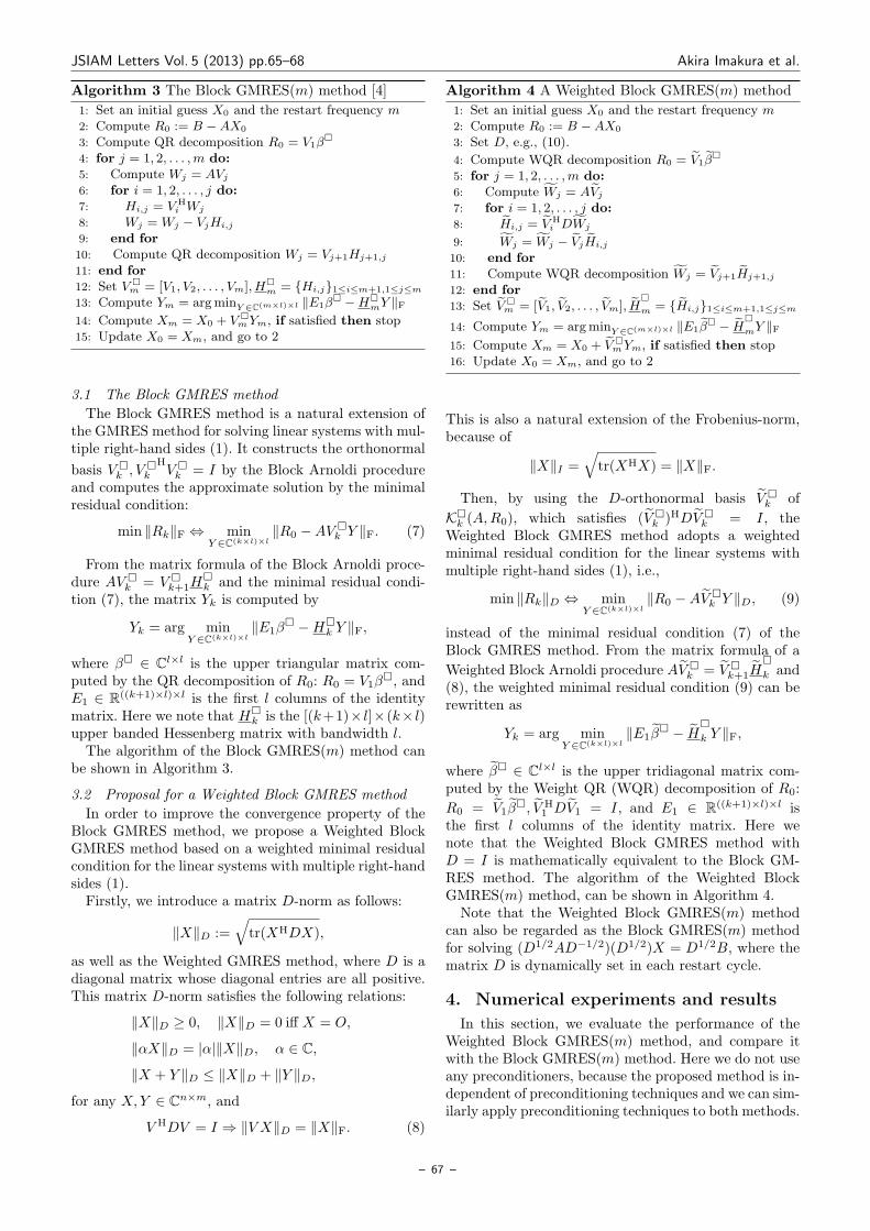
JSIAM Letters Vol. 5 (2013) pp.65–68 Akira Imakura et al.
Algorithm 3 The Block GMRES(m) method [4]
1: Set an initial guess X0 and the restart frequency m2: Compute R0 := B −AX0
3: Compute QR decomposition R0 = V1β
4: for j = 1, 2, . . . ,m do:5: Compute Wj = AVj
6: for i = 1, 2, . . . , j do:7: Hi,j = V H
i Wj
8: Wj = Wj − VjHi,j
9: end for10: Compute QR decomposition Wj = Vj+1Hj+1,j
11: end for12: Set V
m = [V1, V2, . . . , Vm],Hm = Hi,j1≤i≤m+1,1≤j≤m
13: Compute Ym = argminY ∈C(m×l)×l ∥E1β −H
mY ∥F14: Compute Xm = X0 + V
mYm, if satisfied then stop15: Update X0 = Xm, and go to 2
3.1 The Block GMRES method
The Block GMRES method is a natural extension ofthe GMRES method for solving linear systems with mul-tiple right-hand sides (1). It constructs the orthonormal
basis V k , V
k
HV k = I by the Block Arnoldi procedure
and computes the approximate solution by the minimalresidual condition:
min ∥Rk∥F ⇔ minY ∈C(k×l)×l
∥R0 −AV k Y ∥F. (7)
From the matrix formula of the Block Arnoldi proce-dure AV
k = V k+1H
k and the minimal residual condi-
tion (7), the matrix Yk is computed by
Yk = arg minY ∈C(k×l)×l
∥E1β −H
k Y ∥F,
where β ∈ Cl×l is the upper triangular matrix com-puted by the QR decomposition of R0: R0 = V1β
, andE1 ∈ R((k+1)×l)×l is the first l columns of the identitymatrix. Here we note that H
k is the [(k+1)× l]×(k× l)upper banded Hessenberg matrix with bandwidth l.The algorithm of the Block GMRES(m) method can
be shown in Algorithm 3.
3.2 Proposal for a Weighted Block GMRES method
In order to improve the convergence property of theBlock GMRES method, we propose a Weighted BlockGMRES method based on a weighted minimal residualcondition for the linear systems with multiple right-handsides (1).Firstly, we introduce a matrix D-norm as follows:
∥X∥D :=√tr(XHDX),
as well as the Weighted GMRES method, where D is adiagonal matrix whose diagonal entries are all positive.This matrix D-norm satisfies the following relations:
∥X∥D ≥ 0, ∥X∥D = 0 iff X = O,
∥αX∥D = |α|∥X∥D, α ∈ C,
∥X + Y ∥D ≤ ∥X∥D + ∥Y ∥D,
for any X,Y ∈ Cn×m, and
V HDV = I ⇒ ∥V X∥D = ∥X∥F. (8)
Algorithm 4 A Weighted Block GMRES(m) method
1: Set an initial guess X0 and the restart frequency m2: Compute R0 := B −AX0
3: Set D, e.g., (10).
4: Compute WQR decomposition R0 = V1β
5: for j = 1, 2, . . . ,m do:6: Compute Wj = AVj
7: for i = 1, 2, . . . , j do:8: Hi,j = V H
i DWj
9: Wj = Wj − VjHi,j
10: end for11: Compute WQR decomposition Wj = Vj+1Hj+1,j
12: end for13: Set V
m = [V1, V2, . . . , Vm], Hm = Hi,j1≤i≤m+1,1≤j≤m
14: Compute Ym = argminY ∈C(m×l)×l ∥E1β − H
mY ∥F
15: Compute Xm = X0 + V mYm, if satisfied then stop
16: Update X0 = Xm, and go to 2
This is also a natural extension of the Frobenius-norm,because of
∥X∥I =√tr(XHX) = ∥X∥F.
Then, by using the D-orthonormal basis V k of
Kk (A,R0), which satisfies (V
k )HDV k = I, the
Weighted Block GMRES method adopts a weightedminimal residual condition for the linear systems withmultiple right-hand sides (1), i.e.,
min ∥Rk∥D ⇔ minY ∈C(k×l)×l
∥R0 −AV k Y ∥D, (9)
instead of the minimal residual condition (7) of theBlock GMRES method. From the matrix formula of a
Weighted Block Arnoldi procedure AV k = V
k+1Hk and
(8), the weighted minimal residual condition (9) can berewritten as
Yk = arg minY ∈C(k×l)×l
∥E1β − H
k Y ∥F,
where β ∈ Cl×l is the upper tridiagonal matrix com-puted by the Weight QR (WQR) decomposition of R0:
R0 = V1β, V H
1 DV1 = I, and E1 ∈ R((k+1)×l)×l isthe first l columns of the identity matrix. Here wenote that the Weighted Block GMRES method withD = I is mathematically equivalent to the Block GM-RES method. The algorithm of the Weighted BlockGMRES(m) method, can be shown in Algorithm 4.Note that the Weighted Block GMRES(m) method
can also be regarded as the Block GMRES(m) methodfor solving (D1/2AD−1/2)(D1/2)X = D1/2B, where thematrix D is dynamically set in each restart cycle.
4. Numerical experiments and results
In this section, we evaluate the performance of theWeighted Block GMRES(m) method, and compare itwith the Block GMRES(m) method. Here we do not useany preconditioners, because the proposed method is in-dependent of preconditioning techniques and we can sim-ilarly apply preconditioning techniques to both methods.
– 67 –

JSIAM Letters Vol. 5 (2013) pp.65–68 Akira Imakura et al.
Table 1. Convergence results (Restart : number of restart cycle,trestart : computation time per restart, ttotal : total computation
time, TRR : True Relative Residual) of the Block GMRES(m)method and the Weighted Block GMRES(m) method.
Method Restart Time [sec.] TRRtrestart ttotal
COUPLED
Bl-GMRES † 2.48E-01 8.26E+02 -5.05W-Bl-GMRES 1526 2.48E-01 3.79E+02 -12.03
FEM 3D THERMAL1
Bl-GMRES 15 4.36E-01 6.54E+00 -12.44
W-Bl-GMRES 13 4.35E-01 5.66E+00 -12.71
MEMPLUS
Bl-GMRES 393 3.96E-01 1.56E+02 -12.00W-Bl-GMRES 161 3.99E-01 6.42E+01 -12.01
NS3DA
Bl-GMRES 111 8.42E-01 9.35E+01 -12.08
W-Bl-GMRES 121 8.43E-01 1.02E+02 -12.07
4.1 Numerical experiments
For the test problems, we use the following matri-ces: COUPLED (n = 11341, Nnz = 98523) of thecircuit simulation; FEM 3D THERMAL1 (n = 17880,Nnz = 430740) of the thermal problem; MEMPLUS(n = 17758, Nnz = 126150) of the circuit simulation;NS3DA (n = 20414, Nnz = 1679599) of the fluid dy-namics, which are obtained from [9].We set the number of linear systems l = 4 and
the restart frequency m = 30. We also set B as arandom matrix for the right-hand sides, X0 = O forthe initial guess, and the stopping criterion was set as∥Rk∥F/∥B∥F ≤ 10−12. The weight matrix D of theWeighted Block GMRES(m) method was set as follows:
D = diag(d), di =
√n
∥R0∥F
√√√√ n∑j=1
|(R0)i,j |2, (10)
where D was normalized such that ∥D∥F = ∥I∥F =√n.
This is a natural extension of (6), because it is equivalentto (6) in the case of l = 1.The numerical experiments were carried out in double
precision arithmetic on OS: CentOS 64bit, CPU: IntelXeon X5550 2.67GHz (1 core), Memory: 48GB, Com-piler: GNU Fortran ver. 4.1.2, Compile option: -O3.
4.2 Numerical results
We present the numerical results in Table 1. In thistable, a symbol † denotes that the method did not con-verge within 100000 iterations.From Table 1, we can see that the Weighted
Block GMRES(m) method shows almost the same ormore efficient convergence property than the BlockGMRES(m) method. Especially, for COUPLED, theBlock GMRES(m) method did not converge within the100000 iterations; on the other hand, the Weighted BlockGMRES(m) method could obtain the approximate so-lution satisfies required accuracy ∥Rk∥F/∥B∥F ≤ 10−12
with much smaller number of iterations.In terms of the computation time per restart cycle
(trestart), we can also observe that the Block GMRES(m)method and the Weighted Block GMRES(m) methodhave almost the same trestart. This derives from the
fact that the incremental cost of the Weighted BlockGMRES(m) method per restart cycle is only for compu-tations with respect to the matrix D, which is relativelysmaller than for the matrix operation with respect to A.In terms of the total computation time (ttotal), from
the better convergence property and almost the samecomputation time per restart, the Weighted BlockGMRES(m) method could solve the linear systems withmultiple right-hand sides with the less computation timethan the Block GMRES(m) method.
5. Conclusions
In this paper, in order to improve the convergenceof the Block GMRES method, we have proposed theWeighted Block GMRES method based on the weightedminimal residual condition (9) for solving the linear sys-tems with multiple right-hand sides (1). From our nu-merical experiments, we have learned that the WeightedBlock GMRES(m) method is more robust than theBlock GMRES(m) method.For future work, we will compare the proposed
method with other methods, e.g., the Weighted GlobalGMRES(m) method. We also need to investigate thespecific definition of D for efficient convergence.
Acknowledgments
The authors would like to thank Prof. Yusaku Ya-mamoto of Kobe University for his useful comments. Wealso grateful to the referee for valuable suggestions. Thiswork is supported in part by SPIRE Field 5 “The originof matter and the universe”, JST/CREST and KAK-ENHI (Grant No. 22700003).
References
[1] K. Jbilou, A.Messaoudi and H. Sadok, Global FOM and GM-
RES algorithms for matrix equations, Appl. Numer. Math.,31 (1999), 49–63.
[2] M. Heyouni and A. Essai, Matrix Krylov subspace methodsfor linear systems with multiple right-hand sides, Numer. Al-
gorithms, 40 (2005), 137–156.[3] A. El Guennouni, K. Jbilou and H. Sadok, A block version of
BiCGSTAB for linear systems with multiple right-hand sides,Electron. Trans. Numer. Anal., 16 (2003), 129–142.
[4] B. Vital, Etude de quelques methodes de resolution deproblemes lineaires de grande taille sur multiprocesseur, Ph.D. thesis, Univ. de Rennes I. Rennes, France, 1990.
[5] Y. Saad and M. H. Schultz, GMRES: A generalized minimal
residual algorithm for solving nonsymmetric linear systems,SIAM J. Sci. Stat. Comput., 7 (1986), 856–869.
[6] A. Essai, Weighted FOM and GMRES for solving nonsym-
metric linear systems, Numer. Algorithms, 18 (1998), 277–292.
[7] M. H. Gutknecht, Block Krylov space methods for linearsystems with multiple right-hand sides: an introduction, in:
Modern Mathematical Models, Methods and Algorithms forReal World Systems, A. H. Siddiqi et al. eds., pp. 420–447,Anamaya Publishers, New Delhi, India, 2007.
[8] H. Tadano and T. Sakurai, Numerical solvers for solving lin-
ear systems with multiple right-hand sides (in Japanese),OYOSURI, 21 (2011), 276–288.
[9] The University of Florida Sparse Matrix Collection, http:
//www.cise.ufl.edu/research/sparse/matrices/.
– 68 –

JSIAM Letters Vol.5 (2013)
ISBN : 978-4-9905076-4-0
ISSN : 1883-0609
©2013 The Japan Society for Industrial and Applied Mathematics
Publisher :
The Japan Society for Industrial and Applied Mathematics
4F, Nihon Gakkai Center Building
2-4-16, Yayoi, Bunkyo-ku, Tokyo, 113-0032 Japan
tel. +81-3-5684-8649 / fax. +81-3-5684-8663