PL-T-92-2015 AD-A257 762Instrumentation Papers, No. 342

THE ROCKET ELECTRIC FIELD SOUNDING(REFS) PROGRAM: PROTOTYPE DESIGN ANDSUCCESSFUL FIRST LAUNCH

J. C. Willett R. K. Longstreth J. J. JonesD. C. Curtis W. RisonA. R. Driesman W. P. Winn DTIC5 OCT29

15 January 1992 992

92-28298I Ell0l111l11 11111111

. . .AL I................... ... O......ITE

PHILLIPS LABORATORYDIRECTORATE OF GEOPHYSICSAIR FORCE SYSTEMS COMMANDHANSCOM AIR FORCE BASE, MA 01731-5000

9• BJ0' 2k 088

"This technical report has been reviewed and is approved for publication"

DONALD D. GRANTHIAM LUBranch Chief

DiviionDirector

This document has been reviewed by the ESD Public Affairs Office (PA) andis releasable to the National Technical Information Service (NITS).

Qualified requesters may obtain additional copies from the Defense TechnicalInformation Center. All others should apply to the National TechnicalInformation Service.

If your address has changed, or if you wish to be removed from the mailinglist, or if the addressee is no longer employed by your organization, pleasenotify PL/IMA, Hanscom AFB, MA 01731-5000. This will assist us inmaintaining a current mailing list.

Do not return copies of this report unless contractual obligation or noticeson a specific document requires that it be returned.

REPORT DOCUMENTATION PAGE Form Approved

I Oc B No. 0704-01d"Public repodirg for thes collection of information is estimnated to average I hour per response, Including the tire for revlewrin instructions, searchirin existing date sources,

gathn egrn ud toan rseta needed, and completing and reviewing the collection of Information. Send omens regarding t burden estate or any o aspect of fh

collection of Information. including suggesne for reducing thIN burden, to Washington Heardquarters Services, Directr• r Inoormation Operations and Reports, 1215 Jefferson

Davis Hthway, Suite 1204, Arlington, VA 22202-4302, and to the Office of Management and Budget, Paperwork Reduction Project (0704-0188), Washington, DC 20503.

1. AGENCY USE ONLY (Leave blank) 2. REPORT DATE 3. REPORT TYPE AND DATES COVERED

15 January 1992 Scientific Dec 89 - Sep 91

4. TITLE AND SUBTITLE S. FUNDING NUMBERS

The Rocket Electric Field Sounding (REFS) Program: PE 61 101FPrototype Design and Successful First Launch ILIROBI

6. AUTHOR(S) PE62101F

J.C. Willett, D.C. Curtis, A.R. Driesman, R.K. Longstreth, 66701211

W. Rison*, W.P. Winn*, and J.J. Jones*

7. PERFORMING ORGANIZATION NAME(S) AND ADDRESS(ES) 8. PERFORMING ORGANIZATION

REPORT NUMBER

Phillips Laboratory, GPAA PL-TR-92-2015Hanscom AFB, MA 01731-5000 IP. No. 342

9. SPONSORING/MONITORING AGENCY NAME(S) AND ADDRESS(ES) 10. SPONSORINGIMONITORINGAGENCY REPORT NUMBER

11. SUPPLEMENTARY NOTES

* New Mexico Institute of Mining and Technology,

Socorro, NM 87801

12a. DISTRIBUTION/AVAILABILITY STATEMENT 12b. DISTRIBUTION CODE

Approved for Public Release,Distribution Unlimited

13. ABSTRACT (Max~imum 200 words)

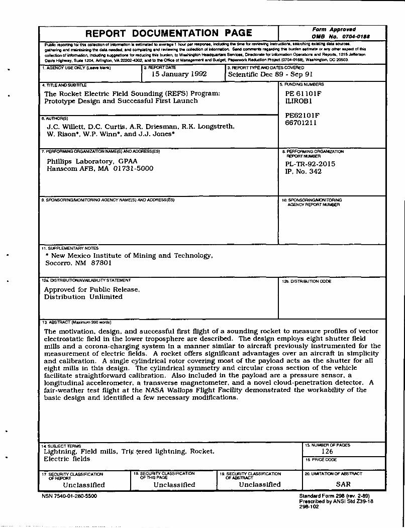
The motivation, design, and successful first flight of a sounding rocket to measure profiles of vectorelectrostatic field in the lower troposphere are described. The design employs eight shutter fieldmills and a corona-charging system in a manner similar to aircraft previously instrumented for themeasurement of electric fields. A rocket offers significant advantages over an aircraft in simplicityand calibration. A single cylindrical rotor covering most of the payload acts as the shutter for alleight mills in this design. The cylindrical symmetry and circular cross section of the vehiclefacilitate straightforward calibration. Also included in the payload are a pressure sensor, alongitudinal accelerometer, a transverse magnetometer, and a novel cloud-penetration detector. Afair-weather test flight at the NASA Wallops Flight Facility demonstrated the workability of thebasic design and identified a few necessary modifications.

14. SUBJECT TERMS 15, NUMBER OF PAGES

Lightning, Field mills, Trigsered lightning, Rocket. 126Electric fields 16 PRICE CODE

17. SECURITY CLASSIFICATION IS. SECURITY CLASSIFICATION 19. SECURITY CLASSIFICATION 20. LIMITATION OF ABSTRACT

OFREPORT OF THIS PAGE OF ABSTRACT

Unclassified Unclassified Unclassified SAR

NSN 7540-01-280-5500 Standard Form 298 (rev. 2-89)Prescribed by ANSI Std Z39-18298-102

Preface

The authors extend sincere thanks to Peter Martini and his expert crew at NASA/WFF for

their help in achieving a successful test flight. The WFF radar and telemetry operators deserve

special mention for their superb job of acquiring our small and rapidly accelerated vehicle.

SSgt. James Anderson of PL/LC did much of the assembly and testing of the payloads and was

an invaluable participant in the field deployment to WFF. Michelle Champion of RADC

designed a first-rate telemetry antenna for the payload, and the Physical Science Laboratory of

NMSU measured its radiation pattern. Wentworth Institute did an excellent Job of mechanical

layout and construction. Capt. Carl Frushon of PL/LC and Dr. George Jumper of Worchester

Polytechnic Institute helped with the aerodynamic and trajectory analysis. William Jafferls

of KSC lent invaluable support and encouragement. Funding for this effort was provided in

part by the Air Force Office of Scientific Research.

Aer!.,:-'cu For

"NTIS C"B l•'°• TIE 0

SU-;~'.n . e d 0

qUALTry n8pECTED a Ju t lt icatlo ,

!Distri-bilt on/

.A .r'i•Itty Codes

.'- and/orDist iSpcial

Dedication

This report is dedicated to the memory of J.J. (Dan) Jones, whose death in an automobilleaccident on November 15, 1991, was a shock to us aH. Dan's enthusiasm energy. and goodnature made him a pleasure to work with and an asset to any project. He will be sorelymissed.

V

Contents

1. INTRODUCTION 1

1.1 Background 11.2 Triggering Conditions 31.3 Planned Approach 8

2. CONCEPTUAL DESIGN OF PAYLOAD 10

2.1 Overview 102.2 Implementation 11

3. ELECTRONIC DESIGN 14

3.1 Stator Charge Amplifier 153.2 Pressure Sensor 153.3 Accelerometer 193.4 Magnetic Field Sensor 193.5 Optical Sensors 233.6 High Voltage Supply and Control 233.7 PCM Encoder 263.8 RF System 283.9 DC-DC Converters 343.10 Batteries 343.11 Internal/External Power Circuits and Ground Support Equipment 37

4. MECHANICAL DESIGN 37

4.1 Rocket Motor 404.2 Rotor/Electronics Section 404.3 High Voltage Section 494.4 Launcher 54

vii

5. PRE-FLIGHT AERODYNAMIC ANALYSIS 57

5.1 Computation of the Mass Properties 575.2 Determination of the Aerodynamic Stability 585.3 Predicted Performance and Dispersion Analysis 60

6. FIELD-MEASUREMENT THEORY AND CAUBRATION 72

6.1 Theory of Measurement 726.2 Laboratory Calibration 74

6.2.1 Potential Calibration 766.2.2 Longitudinal Field Calibration 78

6.3 Theoretical Calibration 816.4 Summary of Matrix Coefficients 84

7. TEST FLIGHT 84

7.1 Post-Flight Aerodynamic Analysis 847.2 Payload Mechanical Performance 857.3 Payload Electrical Performance 95

7.3.1 Charging System 957.3.2 Field Mills 95

7.3.2.1 Stator-Charging Events 987.3.2.2 Noise Levels 987.3.2.3 Fields Prior to Launch 1017.3.2.4 Response to Charging System 1037.3.2.5 In-Flight Potential Calibration 103

7.3.3 Supporting Sensors 1057.3.3.1 Battery and Power System 1057.3.3.2 PCM Encoder 1067.3.3.3 RF System 106

8. CONCLUSIONS AND FUTURE PLANS 108

REFERENCES 111

viii

Illustrations

1. Histogram of Occurrence (White) and Non-occurrence (Hatched) of Triggered 5Lightning Plotted Against Surface Field Intensity

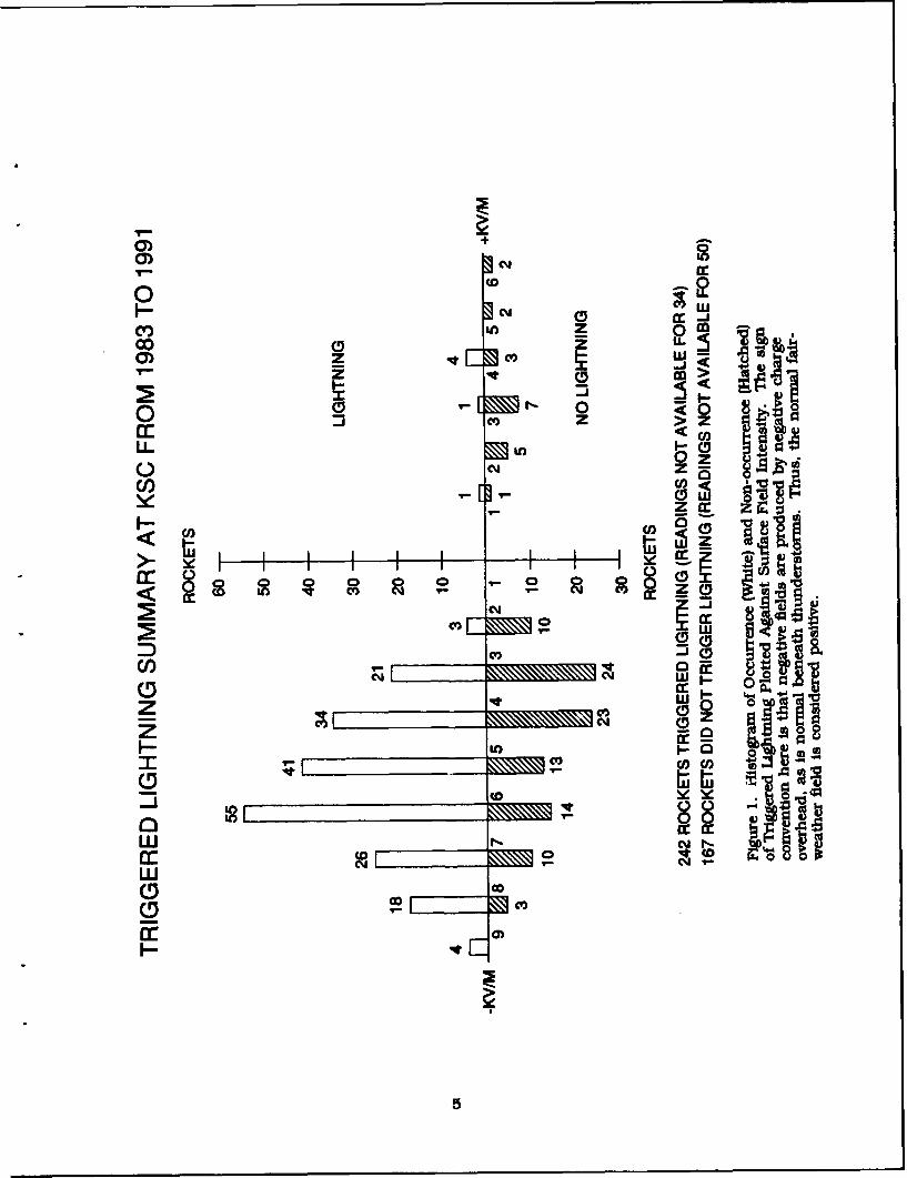
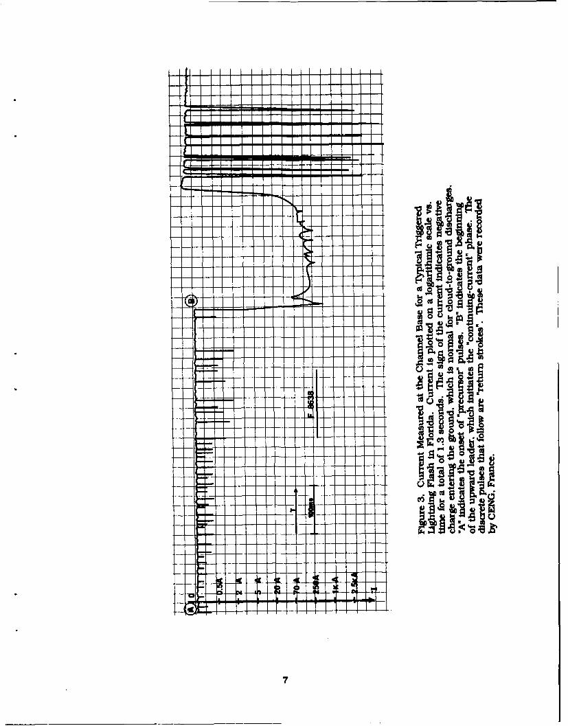
2. Schematic Illustration of the Equipotential Surfaces in the Lowest 200 m and Their 6Interaction With a "Classical" Rocket

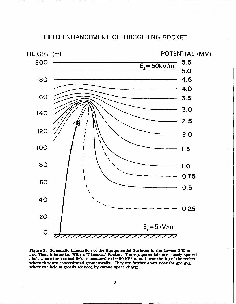
3. Current Measured at the Channel Base for a Typical Triggered Lightning Flash in 7Florida

4. Schematic Illustration of the REFS Payload Mounted on its Rocket Motor 12

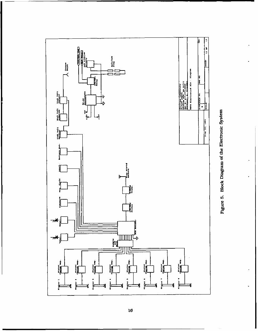
5. Block Diagram of the Electronic System 16

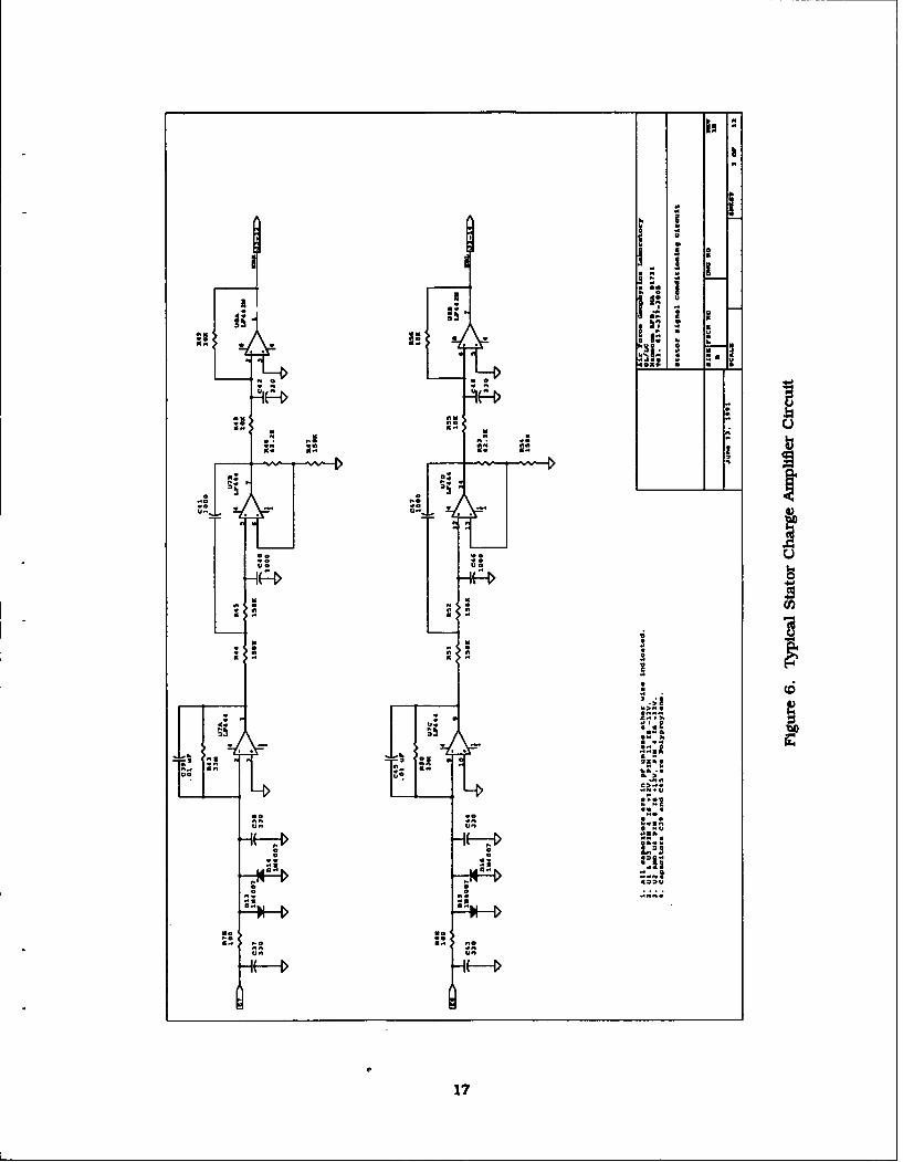
6. Typical Stator Charge Amplifier Circuit 17

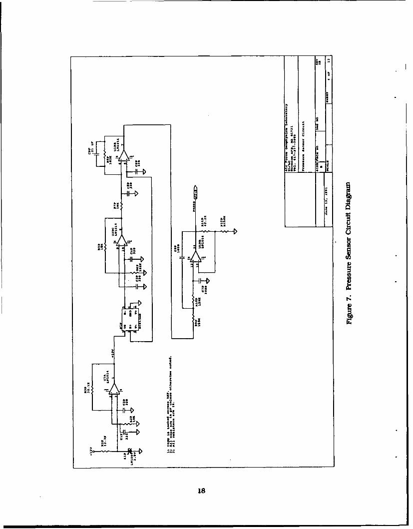
7. Pressure Sensor Circuit Diagram 18

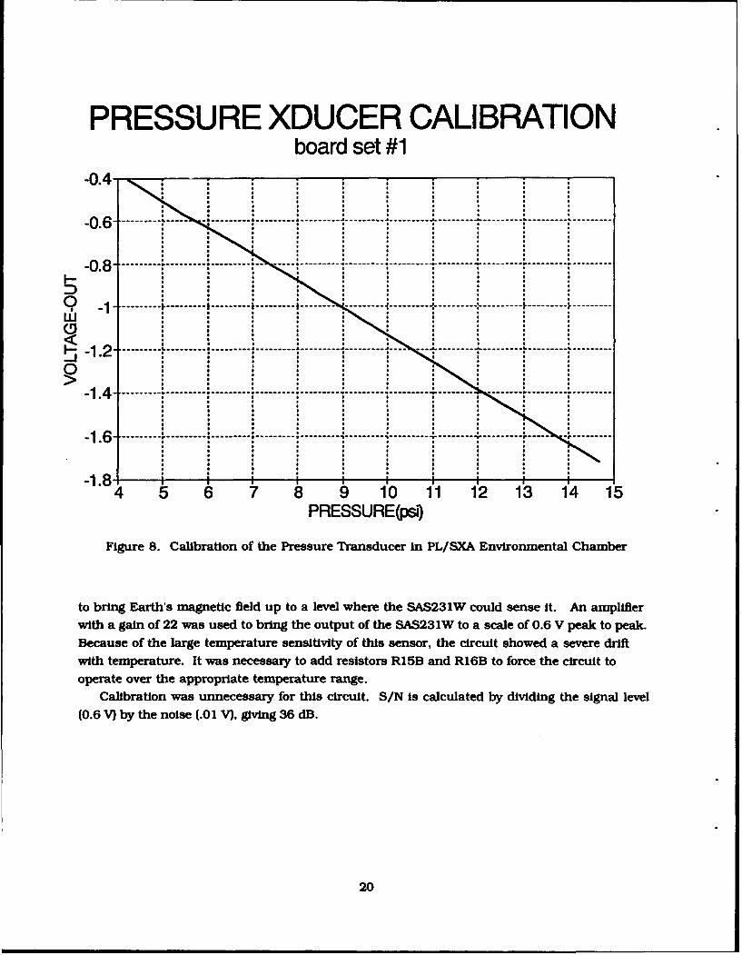
8. Calibration of the Pressure Transducer in PL/SXA Eavironmental Chamber 20

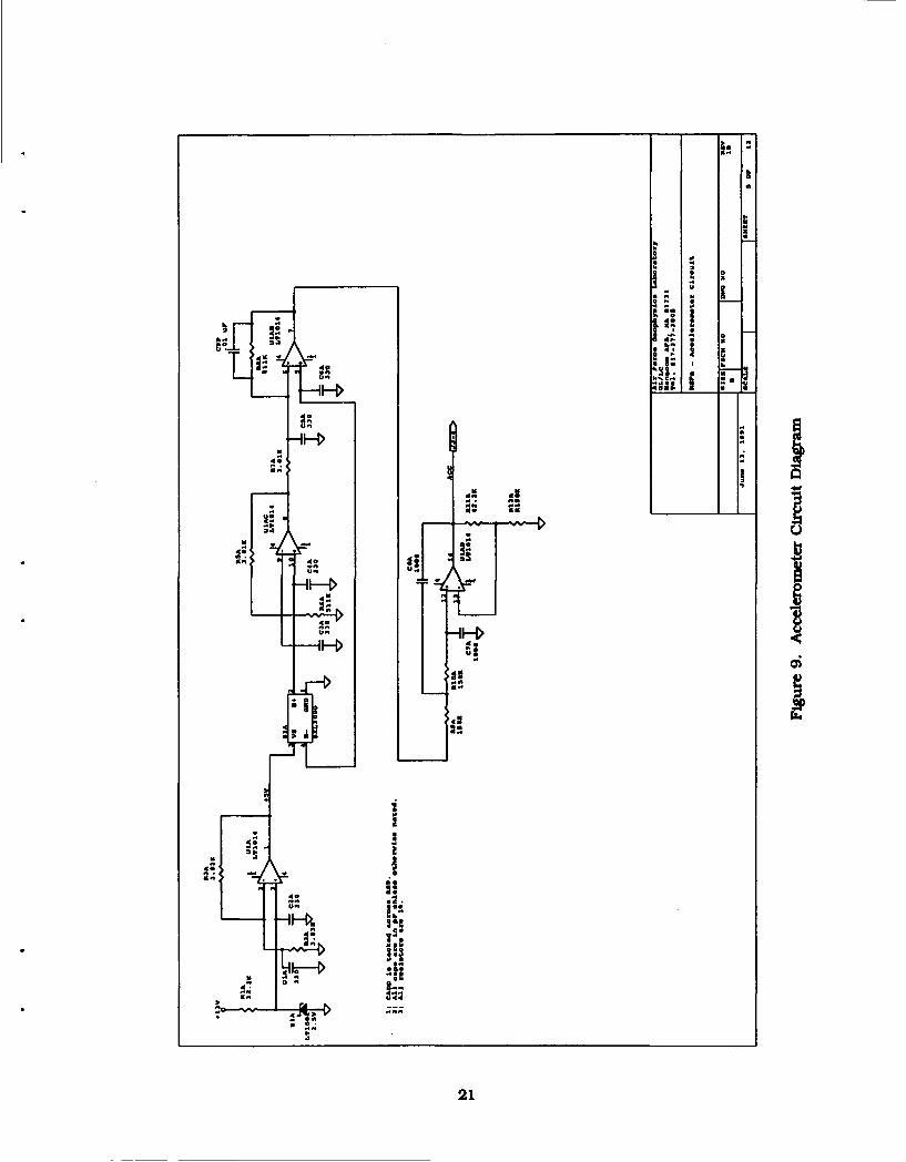
9. Accelerometer Circuit Diagram 21

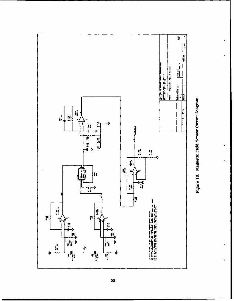
10. Magnetic Field Sensor Circuit Diagram 22

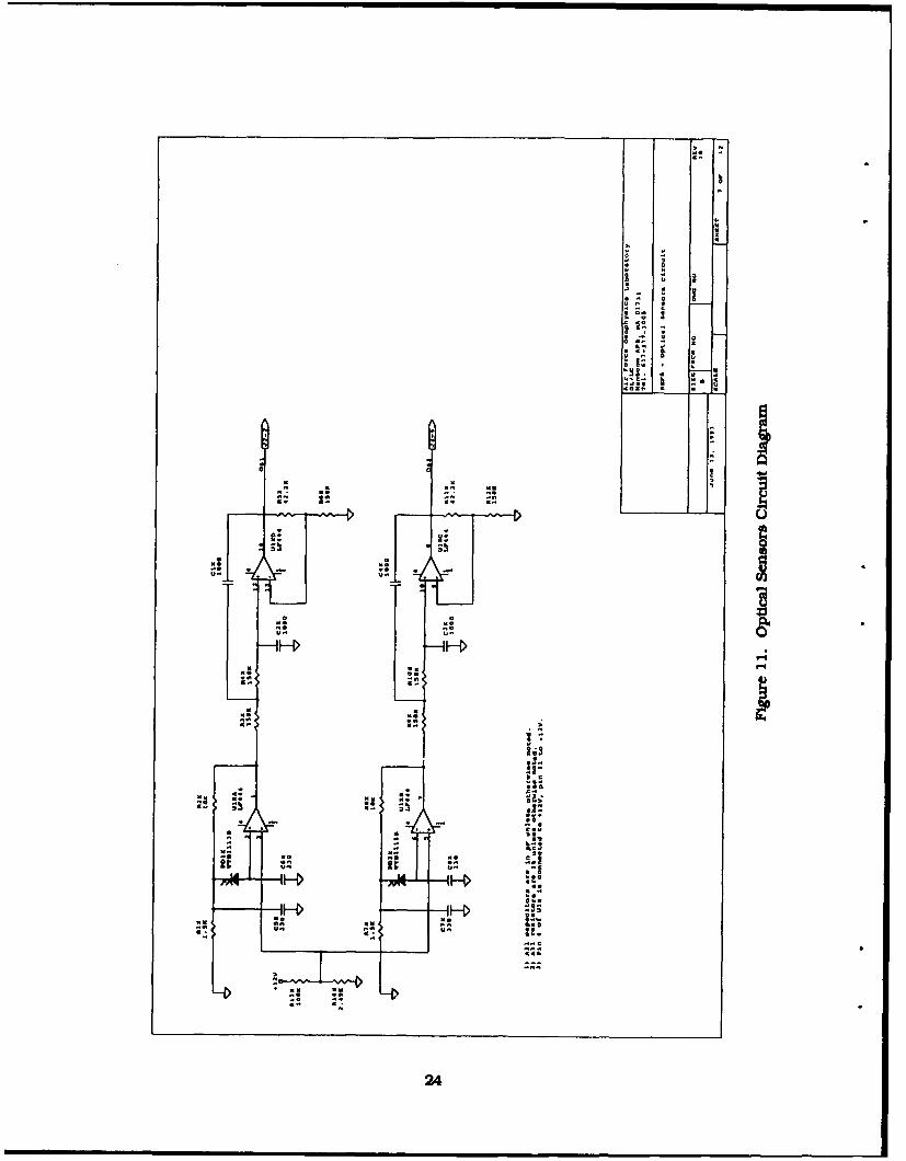
11. Optical Sensors Circuit Diagram 24

12. High Voltage System Circuit Diagram 25

13. PCM Encoder Circuit Diagram 27

14. Control Circuitry Timing Diagram 29

15. Printed-cIrcult-board Layout for the S-band Patch Antenna 31

ix

16a. Measured Intensity of Right-circuitry Polarized Radiation From the REFS Antenna 32

16b. Similar to Figure 16a, but Plotted as a Function of Latitude Angle in the Meridional 33Plane (Including the Payload Axis)

17. DC-DC Converter Circuit Diagram 35

18. REFS Battery Connection Diagram 36

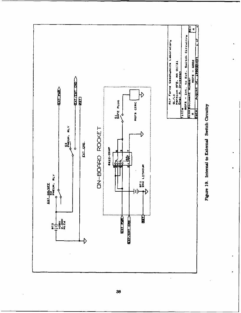
19. Internal to External Switch Circuitry 38

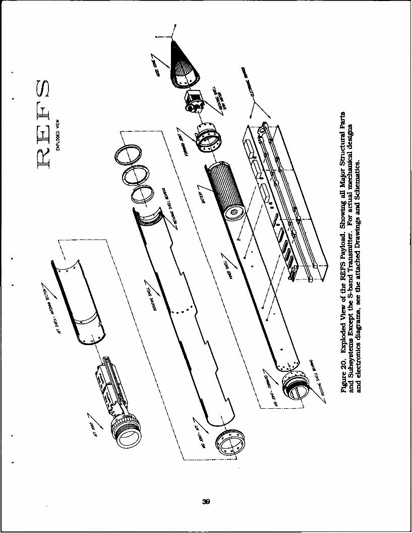
20. Exploded View of the REFS Payload, Showing all Major Structural Parts and 39Subsystems Except the S-band Transmitter

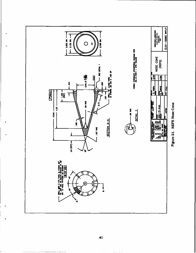
21. REFS Nose Cone 41

22. Detail of the Nose Cone, Forward Joint, and Spin Motor 42

23. Motor Mounting Plate and Gearing 43

24. Rotating Shell 45

25. Detail of the Forward End of the Rotating Shell, Showing the Forward Bearing 46Mounting

26. Detail of the Mid-Joint, Showing the Mounting of the Aft Bearing and the Aft End 47of the Inner Shell

27. Stator Shell Mid-section 48

28. Battery Container Assembly 50

29. Aft Shell 51

30. Detail of the High-voltage Section, Showing the Aft Joint, Mounting Brackets for the 52High-voltage Power Supplies and S-band Transmitter (not Shown), and the Aft Shellthat Carries the Telemetry Antenna

31. Base Ring Aft Section 53

32. Umbilical Bracket - Aft Section 55

33. Forward Ring Mid-section 56

34. The Output of the Top-right Mill When +10 kv is Applied to the Payload 75

35. Stator Calibration Circuit 77

36. Charge Amplifier Circuit Diagram 80

37 Altitude vs Time Predicted and Observed (Observed Trajectory Begins About 8 Seconds 86After Launch Because of Delays in Radar Acquisition) for the REFS Flight on5 Nov 91 From WFF

38. Range vs Time Predicted and Observed (Observed Trajectory Begins About 8 Seconds 87After Launch Because of Delays in Radar Acquisition) for the REFS Flight on5 Nov 91 From WFF

39. Velocity vs Time Predicted and Observed (Observed Trajectory Begins About 8 Seconds 88After Launch Because of Delays in Radar Acquisition) for the REFS Flight on5 Nov 91 From WFF

40. Altitude vs Range Predicted and Observed (Observed Trajectory Begins at About 7700 ft 89Altitude Because of Delays in Radar Acquisition) for the REFS Flight on5 Nov 91 From WFF

x

41. Vehicle Spin Rate Around its Longitudinal Axis (Determined From the Magnetic Field 90Sensor) as a Function of Time During the First Six Seconds of the REFS Flight on5 Nov 91 From WFF

42. Vehicle Spin Rate Around its Longitudinal Axis (Determined From the Magnetic 91Field Sensor) as a Function of Time During the Entire REFS Flight on5 Nov 91 From WFF

43. Altitude Determined From the Pressure Transducer, Compared With Altitude From the 92Tracking Radars, as a Function of Time for the REFS Flight on 5 Nov 91 from WFF

44. Outer Shell (Rotor) Rotation Rate (Determined From the Optical Detectors), Compared 93With Vehicle Spin Rate, as a Function of Time During the First Six Seconds of theREFS Flight on 5 Nov 91 From WFF

45. Outer Shell (Rotor) Rotation Rate (Determined From the Optical Detectors), Compared 94With Vehicle Spin Rate, as a Function of Time During the Entire REFS Flight on5 Nov 91 From WFF

46. HIgh Voltage Timing Diagram 96

47. Overview of the Entire REFS Flight on 5 Nov 91 97

48. The Outputs of all of the Mills During the Period of Maximum Field in the REFS Flight 99of 5 Nov 91

49. A Magnification of MT (top) and MB (Bottom) From Figure 48, Showing the 100Difference in Noise Waveforms

50. Photograph of the REFS Vehicle in its Launch Tube at WFF 102

51. The Effect of a Typical Negative-polarity Corona Pulse on Four of the Field Mills 104

52. Power-supply Voltage as a Function of Time During the Flight on 5 Nov 91 From WFF 107

53. Corona Point (REFS) 109

xi

Tables

1. Range Calculations for REPS Wallops-Island Launch 30

2. Summary of REFS Mass Properties 58

3. Aerodynamic Stability Derivatives 59

4. Predicted Performance and Dispersion Analysis 60

5. GL REFS 2.75 Inch, QE = 75 Degrees, Representative Trajectories 62

6. GL REFS 2.75 Inch, QE = 75 Degrees, Dispersion 63

7. Field-mill Outputs vs Applied Potential and Stator Charge 76

8. Estimates of Longitudinal Field Coefficients af 81

9. Analytic and Measured Field and Potential Coefficients 83

10. MIDl Outputs, Stator Calibration, and Field Intensity 101

11. Analytic and Measured Field and Apparent E. 101

12. MiIl Outputs, Stator Charge, and Apparent Potential 105

xii

The Rocket Electric Field Sounding (REFS) Program:Prototype Design and Successful First Launch

1. INTRODUCTION

1.1 Background

The physics of lightning in general, and of triggered lightning in particular, is not

understood. 'Triggering" is defined here as the artificial (intentional or inadvertent) initiation

of a lightning discharge by the rapid introduction of a conducting body into a region of high

electrostatic field. A triggered discharge begins with a "leader" -- a self-propagating, highly

ionized channel extending into virgin air -- initiated at, and propagating away from, the

triggering object. Inadvertent triggered lightning is a severe threat to aerospace operations, as

illustrated by the Atlas/Centaur-67 disaster1 on March 26, 1987. On this occasion an un-

manned booster carying a Navy communications satellite was destroyed as the result of a

direct lightning strike about 49 seconds after launch from the Eastern Test Range at Cape

Canaveral, Florida. It is now known that the vast majority of lightning strikes to aircraft and

minssiles in flight are triggered. 2 ,3

Received for publication 13 Jan 1992

1 NASA Goddard Space Flight Center (1987) Atlas/Centaur-67 FLTSATCOM F-6 InvestigationBoard, Report, NASA Goddard Space Flight Center, Greenbelt, MD 20771, 15 July 1987.

2 Mazur, V., Fisher, B.D., and Gerlach, J.C. (1984) l~ghtning Strikes to an airplane in athunderstorm, J. Aircraft, 21:607-611.

..1 .. .-..... .... ..

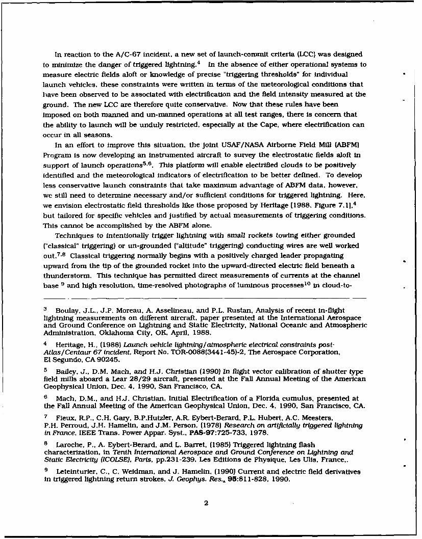
In reaction to the A/C-67 incident, a new set of launch-commit criteria (LC) was designed

to minimize the danger of triggered lightning. 4 In the absence of either operational systems to

measure electric fields aloft or knowledge of precise "triggering thresholds" for individual

launch vehicles, these constraints were written in terms of the meteorological conditions that

have been observed to be associated with electrification and the field intensity measured at the

ground. The new LCC are therefore quite conservative. Now that these rules have been

imposed on both manned and un-manned operations at all test ranges, there is concern that

the ability to launch will be unduly restricted, especially at the Cape, where electrification can

occur in all seasons.

In an effort to improve this situation, the joint USAF/NASA Airborne Field Mill (ABFM)

Program Is now developing an instrumented aircraft to survey the electrostatic fields aloft in

support of launch operations5 .6 . This platform will enable electrified clouds to be positively

identified and the meteorological indicators of electrification to be better defined. To develop

less conservative launch constraints that take maximum advantage of ABFM data. however,

we still need to determine necessary and/or sufficient conditions for triggered lightning. Here,

we envision electrostatic field thresholds like those proposed by Heritage [1988, Figure 7.11,4

but tailored for specific vehicles and justified by actual measurements of triggering conditions.

This cannot be accomplished by the ABFM alone.

Techniques to Intentionally trigger lightning with small rockets towing either grounded

("classical" triggering) or un-grounded ("altitude" triggering) conducting wires are well worked

out.7 .8 Classical triggering normally begins with a positively charged leader propagating

upward from the tip of the grounded rocket into the upward-directed electric field beneath a

thunderstorm. This technique has permitted direct measurements of currents at the channel

base 9 and high resolution, time-resolved photographs of luminous processes1 0 in cloud-to-

3 Boulay, J.L., J.P. Moreau, A. Asselineau, and P.L. Rustan, Analysis of recent in-flightlightning measurements on different aircraft, paper presented at the International Aerospaceand Ground Conference on Lightning and Static Electricity, National Oceanic and AtmosphericAdministration, Oklahoma City, OK, April, 1988.

4 Heritage, H., (1988) Launch vehicle lightning/atmospheric electrical constraints post-Atlas/Centaur 67 incident, Report No. TOR-0088(3441-45)-2, The Aerospace Corporation,El Segundo, CA 90245.

5 Bailey, J., D.M. Mach, and H.J. Christian (1990) In flight vector calibration of shutter typefield mills aboard a Lear 28/29 aircraft, presented at the Fall Annual Meeting of the AmericanGeophysical Union, Dec. 4, 1990, San Francisco, CA.

6 Mach, D.M., and H.J. Christian, Initial Electrification of a Florida cumulus, presented at

the Fall Annual Meeting of the American Geophysical Union, Dec. 4, 1990, San Francisco, CA.

7 Fleux, R.P., C.H. Gary, B.P.Hutzler, A.R. Eybert-Berard, P.L. Hubert, A.C. Meesters.P.H. Perroud, J.H. Hamelin, and J.M. Person, (1978) Research on artificlally triggered lightningin France, IEEE Trans. Power Appar. Syst., PAS-97:725-733, 1978.

8 Laroche, P., A. Eybert-Berard, and L. Barret, (1985) Triggered lightning flashcharacterization, in Tenth International Aerospace and Ground Conference on Lightning andStatic Electricity (ICOLSE), Paris, pp. 2 3 1-239, Les Editions de Physique, Les Ulis, France,.

9 Leteinturier, C., C. Weidman, and J. Hamelin, (1990) Current and electric field derivativesin triggered lightning return strokes, J. Geophys. Res., 95:811-828, 1990.

2

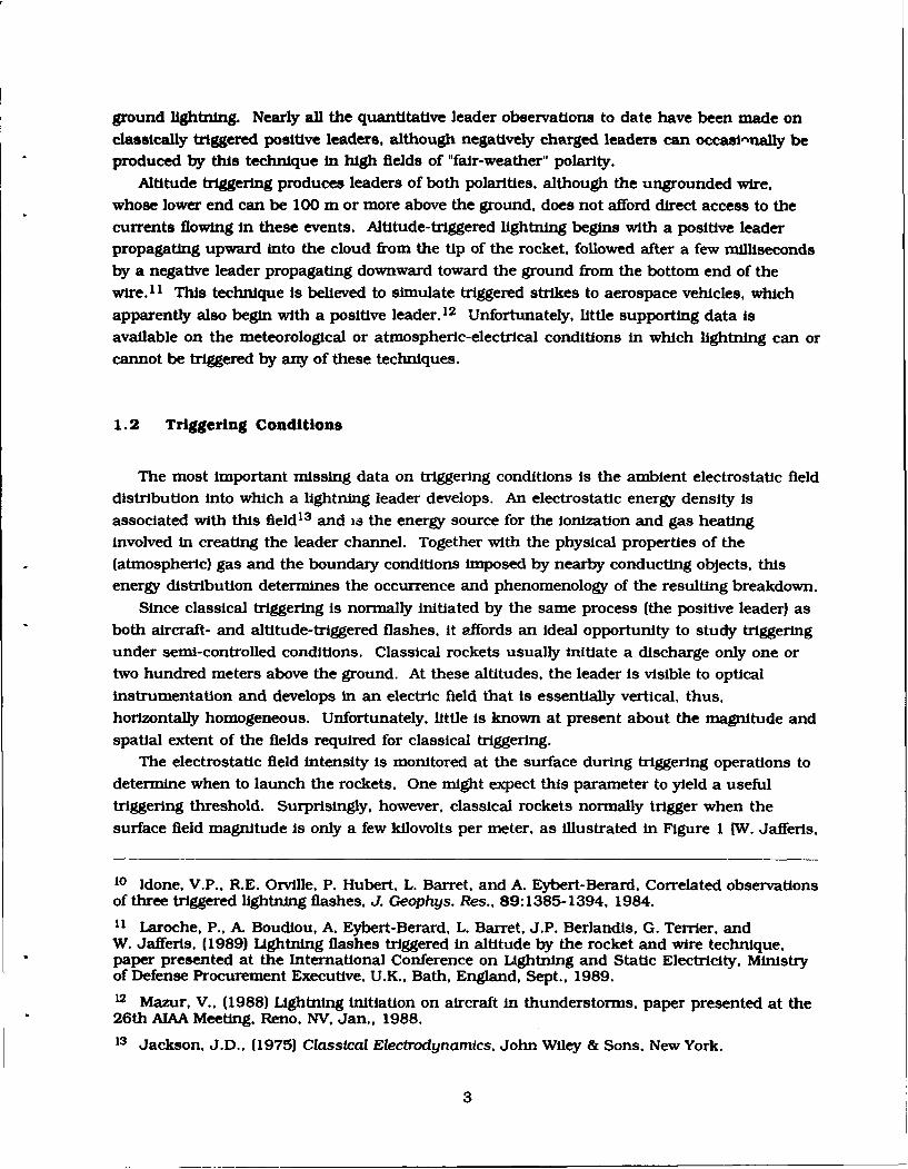
ground lightning. Nearly all the quantitative leader observations to date have been made onclassically triggered positive leaders, although negatively charged leaders can occasiunamly beproduced by this technique in high fields of "fair-weather" polarity.

Altitude triggering produces leaders of both polarities, although the ungrounded wire,whose lower end can be 100 m or more above the ground, does not afford direct access to thecurrents flowing In these events. Altitude-triggered lightning begins with a positive leaderpropagating upward into the cloud from the tip of the rocket, followed after a few millisecondsby a negative leader propagating downward toward the ground from the bottom end of thewire. 11 This technique is believed to simulate triggered strikes to aerospace vehicles, whichapparently also begin with a positive leader. 12 Unfortunately, little supporting data isavailable on the meteorological or atmospheric-electrical conditions in which lightning can orcannot be triggered by any of these techniques.

1.2 Triggering Conditions

The most important missing data on triggering conditions Is the ambient electrostatic fielddistribution into which a lightning leader develops. An electrostatic energy density isassociated with this field 13 and is the energy source for the ionization and gas heatingInvolved in creating the leader channel. Together with the physical properties of the(atmospheric) gas and the boundary conditions imposed by nearby conducting objects, thisenergy distribution determines the occurrence and phenomenology of the resulting breakdown.

Since classical triggering is normally initiated by the same process (the positive leader) asboth aircraft- and altitude-triggered flashes, it affords an Ideal opportunity to study triggeringunder semi-controlled conditions. Classical rockets usually initiate a discharge only one ortwo hundred meters above the ground. At these altitudes, the leader is visible to opticalinstrumentation and develops in an electric field that is essentially vertical, thus,horizontally homogeneous. Unfortunately, little is known at present about the magnitude andspatial extent of the fields required for classical triggering.

The electrostatic field intensity is monitored at the surface during triggering operations todetermine when to launch the rockets. One might expect this parameter to yield a usefultriggering threshold. Surprisingly, however, classical rockets normally trigger when thesurface field magnitude is only a few kilovolts per meter, as illustrated in Figure 1 [W. Jafferis,

10 Idone. V.P., R.E. Orville, P. Hubert, L. Barret, and A. Eybert-Berard, Correlated observationsof three triggered lightning flashes, J. Geophys. Res., 89:1385-1394, 1984.

11 Laroche, P., A. Boudiou, A. Eybert-Berard, L. Barret, J.P. Berlandis, G. Terrier, andW. Jafferis, (1989) Lightning flashes triggered in altitude by the rocket and wire technique,paper presented at the International Conference on iUghtning and Static Electricity. Ministryof Defense Procurement Executive, U.K., Bath, England, Sept., 1989.

12 Mazur, V., (1988) Lightning initiation on aircraft in thunderstorms, paper presented at the26th AIAA Meeting, Reno, NV, Jan., 1988.

13 Jackson, J.D., (1975) Classical Electrodynamics, John Wiley & Sons. New York.

3

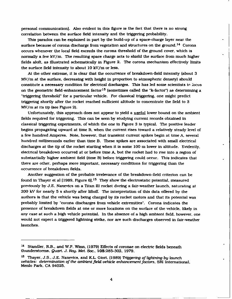
personal communicationi. Also evident in this figure is the fact that there is no strong

correlation between the surface field intensity and the triggering probability.

This paradox can be explained in part by the build-up of a space-charge layer near the

surface because of corona discharge from vegetation and structures on the ground. 14 Corona

occurs whenever the local field exceeds the corona threshold of the ground cover, which is

normally a few ky/m. The resulting space charge acts to shield the surface from much higher

fields aloft, as illustrated schematically in Figure 2. The corona mechanism effectively limits

the surface field intensity to about 10 kV/m or less.

At the other extreme, it is clear that the occurrence of breakdown-field intensity (about 3

MV/m at the surface, decreasing with height in proportion to atmospheric density) should

constitute a necessary condition for electrical discharges. This has led some scientists to ;ocus

on the geometric field-enhancement factor 1 5 (sometimes called the "k-factor") as determining a

"triggering threshold" for a particular vehicle. For classical triggering, one might predict

triggering shortly after the rocket reached sufficient altitude to concentrate the field to 3MV/m at its tip (see Figure 2).

Unfortunately, this approach does not appear to yield a useful lower bound on the ambient

fields required for triggering. This can be seen by studying current records obtained in

classical triggering experiments, of which the one in Figure 3 is typical. The positive leader

begins propagating upward at time B, when the current rises toward a relatively steady level of

a few hundred Amperes. Note, however, that transient current spikes begin at time A, several

hundred milliseconds earlier than time B. These spikes are associated with small electrical

discharges at the tip of the rocket starting when it Is some 100 m lower in altitude. Evidently,

electrical breakdown occurred at or before time A, but the rocket had to rise into a region of

substantially higher ambient field (time B) before triggering could occur. This indicates that

there are other, perhaps more important, necessary conditions for triggering than the

occurrence of breakdown fields.

Another suggestion of the probable irrelevance of the breakdown-field criterion can be

found in Thayer et al [1989, Figure 61.1 5 They show the electrostatic potential, measured

previously by J.E. Nanevics on a Titan III rocket during a fair-weather launch, saturating at

200 kV for nearly 5 s shortly after liftoff. The interpretation of this data offered by the

authors is that the vehicle was being charged by its rocket motors and that its potential was

probably limited by "corona discharges from vehicle extremities". Corona indicates thepresence of breakdown fields at one or more locations on the surface of the vehicle, likely in

any case at such a high vehicle potential. In the absence of a high ambient field, however, onewould not expect a triggered lightning strike, nor are such discharges observed in fair-weather

launches.

14 Standler, R.B., and W.P. Winn, (1979) Effects of coronae on electric fields beneaththunderstorms, Quart. J. Roy. Met. Soc., 105:285-302, 1979.

15 Thayer, J.S., J.E. Nanevics, and K.L. Glori, (1989) Triggering of lightning by launchvehicles: determination of the ambient field vehicle enhancement factors, SRI International,Menlo Park, CA 94025.

4

1;E

0) +0) N~

o Zo

0f) z

0 0

oCV) z>1.-c

I I I IF- 00

C0 0 -08

CV) w

0 0

0 %

FN'

00

CEC0-

05

FIELD ENHANCEMENT OF TRIGGERING ROCKET

HEIGHT (i) POTENTIAL (MV)200 Ez= 50kV/m 5.5

5.0

180 4.5

4.0160 35

140 3.0

2.5

1 I -2.0

100 1.5

80 1.0

60 0.75

0.5

40 -0

00.2520

0 Ez= 5kV/m

Figure 2. Schematic Illustration of the Equlpotential Surfaces in the Lowest 200 mand Their Interaction With a "Classical" Rocket. The equlpotentials are closely spacedaloft, where the vertical field is assumed to be 50 kV/m, and near the tip of the rocket,where they are concentrated geometrically. They are further apart near the ground,where the field is greatly reduced by corona space charge.

6

w11E,

7;

Thus, we are drawn to the conclusion that it is one or more properties of the ambient fielddistribution, probably over some distance along the eventual leader-propagation path, ratherthan the local field intensity at the surface of the rocket, that determines the triggeringconditions.

Several attempts have been made to measure the electric fields associated with lightningstrikes to flying aircraft. 16 .17 The accuracy of such measurements is problematic, however,because of the difficulty of measuring ambient electrostatic fields from aircraft in the hostileenvironment in which the data must be taken. Furthermore, we want not only the magnitudeof the field at the location where the strike occurred, but also the vector component parallel to,and for some distance along, the direction of propagation of the discharge. Obviously, it can bedifficult to determine this direction when the aircraft is flying in cloud and precipitation, andin any case, the aircraft may not be moving in the right direction to obtain this information.

1.3 Planned Approach

The most productive approach to understanding triggering appears to be obtaining near-

instantaneous, vertical profiles of the vertical component of electrostatic ficM'• immediatelyprior to a large number of triggering attempts with both classical and altitude rockets. Suchprofiles, to an altitude of a few kilometers, will allow calculation of the electrostatic energy

available for the visible development of the discharge and will permit identification of anyother features of the spatial distribution of field that might be important in determining thetriggering conditions. Measurements on classical triggering will lead to an understanding of

the initiation and propagation of the positive leader -- the initial process In strikes toaerospace vehicles. Measurements on altitude triggering will facilitate determination of theinfluence of vehicle properties (field-enhancement factor, length, velocity, etc.) on thetriggering conditions. In both cases, it is necessary to obtain the profiles rapidly, so that thefield distribution has no time to change before the triggering rocket Is launched. Soundingballoons ascend too slowly for this purpose. Multiple passes by an instrumented aircraft also

take too long.

In principle, such profiles could be obtained with numerous individual sensors suspendedfrom a tethered balloon. There are two problems with this procedure, however. First, it isdifficult to assure that the tether cable does not influence the measurement. Even tether

materials that are good Insulators when new become weakly conducting with exposure to theweather, especially at a coastal site. 18' 19 Second, there are significant safety and reliability

16 Anderson, R.V., and J.C. Bailey, (1987) Vector electrlc ftelds measured in a lightningenvironment, Memorandum Report 5899, Naval Research Laboratory, Washington, DC 20375.17 Laroche, P.. A. Delannoy, and H. Le Court de Beru, Electrostatic field conditions on anaircraft stricken by lightning, paper presented at the International Conference on Lightningand Static Electricity, Ministry of Defense Procurement Executive, U.K.. Bath, England. Sept..1989.

18 Latham, D.J., (1974) Atmospheric Electrical Effects of an on Tethered Balloon Systems,Report 2176, Advanced Research Projects Agency, Arlington, Va. 22209.

8

problems with operating such a tethered-balloon system in a thunderstorm environment. This

has been tried at KSC with limited success, most recently resulting in the loss of the balloon

and most of the instrumentation in strong winds during August, 1991. It appears that great

effort is required to obtain reliable profiles in this manner on a regular basis. Nevertheless,

we expect to inter-calibrate our profiling instrumentation with such balloon-borne apparatus

on a few occasions.For all of the above reasons, we chose a rocket to make the required measurements.

Rockets have been used successfully by Winn et al.20 to obtain profiles of the transverse

components (perpendicular to the direction of flight) of the electrostatic field. Unfortunately.

these components are much less scientifically interesting than the longitudinal component (in

the direction of flight), and they are not useful for the present purpose. There have been at

least two prior attempts to develop rocket-borne sensors to measure the longitudinal

component of the field. Ruhnke21 designed a corona-discharge sensor for this purpose, but he

was not able to demonstrate Its accuracy and reliability in a thunderstorm environment.Scientists at the Office National d'Etudes et de Recherches Aerospatiales (ONERA) in France

have also made an unsuccessful attempt to produce such a sensor [P. Laroche, personalcommunication].

New electric-fleld-sounding rockets based on shutter field mills are currently under

development by the Geophysics and Aerospace Engineering Directorates (formerly the

Geophysics Laboratory) of the Phillips Laboratory (PL), and separately by ONERA. This report

describes the design, calibration, and successful first flight of our prototype Rocket Electric

Field Sounding (REFS) payload aboard a 2.75-in. Folding-Fin Aircraft Rocket (FFAR) motorcalled the "Mighty Mouse". The intent of the REFS Program is to construct a number of these

payloads and launch them as part of the Rocket-ThIggered-Lightning Program (RTLP) at theKennedy Space Center (KSC), Florida, where triggering operations have been under way since

1984.

It is hoped to use REFS instrumentation in the context of a larger investigation of the

nature of triggering. In addition to electric field soundings, understanding the physics ofleader propagation requires extensive diagnostics of the developing leaders. The goals here are

to unambiguously identify some of the processes observed in triggered lightning with those

occurring in long laboratory sparks and to completely characterize those phenomena notreproducible in the laboratory because their scale size is too large. High resolution optical

observations of geometry, propagation speed, and stepping or non-stepping22 are needed to tellus the dependence of leader behavior on field magnitude. Direct recordings of current at the

19 Jonsson, H.H., (1990) Possible errors in electrical measurements made in thundercloudswith balloon-borne instrumentation, submitted to J. Geophys. Res.20 Winn, W.P., G.W. Schwede, and C.B. Moore, (1974) Measurements of electric fields inthunderclouds, J. Geophys. Res., 79:1761-1767.

21 Ruhnke, L.H., (1971) A Rocket Borne Instrument to Measure Electric Fields Inside ElectrifiedClouds, NOAA/ERL. Boulder, CO. April 1971.

22 Idone, V.P. and R.E. Orville (1988) Channel tortuosity variation in Florida triggeredlightning, Geophys. Res. Lett.. 15:645-648.

9

channel base,23 as well as remote sensing of charge and current distributions in the growing

channel by means of multiple-station, field-change recordings, are important to define the

electrical characteristics of these discharges. Spectroscopic and radar observations would also

yield valuable information about the physics of the leader channels.

2. CONCEPTUAL DESIGN OF PAYLOAD

2.1 Overview

The design of the REFS payload was based on a proposal originally submitted to

NASA/KSC from the New Mexico Institute of Mining and Technology (NMIMT) [Winn, W.P.,

W. Rison, and J.J. Jones, A rocket-borne instrument to measure electric vectors in clouds.

June, 1988, personal communication]. This section describes the overall design articulated in

that proposal, as modified during further development in collaboration with PL.

The driving requirement of the design was to obtain accurate and reliable vertical profilesof the vertical component of electrostatic field E.(z(. This is essentially the longitudinal

component relative to the sounding rocket during most of its flight. The potential importance

of these measurements to flight safely, their difficulty, and the lack of any convincing means

of verification, as discussed above, require that the payload be self-calibrating and incorporate

sufficient redundancy to detect errors in an individual sounding.

Redundancy is essential to rule out several different potential sources of error. Of most

concern is the effect of the exhaust plume from the rocket motor during burn (the lowest few

hundred meters of the profile). A highly conductive plume would tend not only to charge or

discharge the rocket body but also to modify the enhancement factors for ambient field by

changing the electrical geometry of the vehicle. Another significant concern is the effect of

space charge produced by corora from the vehicle in regions of very high electric field.

Charging of the sensors themselveq and charge build-up on the insulators, because of particle

impaction, corona discharge, or some other source, may also occur under certain conditions.

Any of these processes might cause spurious readings that could not be differentiated from real

ambient fields without redundancy.

Calibration of the longitudinal component of the field is made difficult by the facts that

the vehicle is too long to suspend in readily available uniform-field chambers and that in-

flight inter-comparison with other calibrated systems in a high-field environment is

problematic. The NMIMT proposal pointed out the following clever means of self-calibration,

assuming that all three components of the ambient vector field are measured. The components

23 Laroche, P., A. Eybert-Berard, L. Barret, J.P. Berlandis, (1988) Observations of preliminarydischarges Initiating flashes triggered by the rocket and wire technique, paper presented at the8th International Conference on Lightning and Atmospheric Electricity, National ScienceResearch Council, Uppsala, Sweden, June 1988.

10

transverse to the rocket are relatively easy to calibrate because of its small diameter andnearly cylindrical geometry. Since the rocket will arc over fairly rapidly at apogee. whenlaunched at a high elevation angle, it is possible to transfer this calibration from thetransverse to the longitudinal component, provided only that the ambient field near apogee isslowly varying in time and space. The assumption of slow time variability can be verified bythe lack of lightning field changes at field mills on the ground. The assumption of spatialhomogeneity can be supported by the similarity of upward and downward profiles. Thus thelongitudinal component can be calibrated in flight on many of the individual soundings.

The redundancy requirement on the longitudinal field component implies measurements atthree or more longitudinal positions along the rocket body, forcing the choice of shutter fieldmills (as opposed to corona probes or cylindrical mills) as the basic sensors. This choice,together with the need for the transverse field components to satisfy the self-calibrationrequirement, implies a minimum of five such sensors. (It is possible to develop a hybridsystem to meet these requirements. ONERA envisions shutter mills of novel design, eachmeasuring the average radial field at one longitudinal position, plus a cylindrical mill todetermine the two transverse components. Such an approach introduces additionalcomplexities, however.) Having made these choices, we are designing what is essentially anABFM system. The problems involved have been discussed recently by Kositsky et al. ,24

Jones, 25 Bailey and Anderson. 26 and Laroche. 2 7 Theoretically, suitable placement of five millswould allow determination of the three components of ambient field, after removal of theeffects of vehicle charge, and still provide one redundant measurement. Fortunately. the

* almost perfect cylindrical symmetry of a rocket and the flexibility afforded by a custom-designed payload permit more nearly ideal mill locations than are possible on an aircraft.

2.2 Implementation

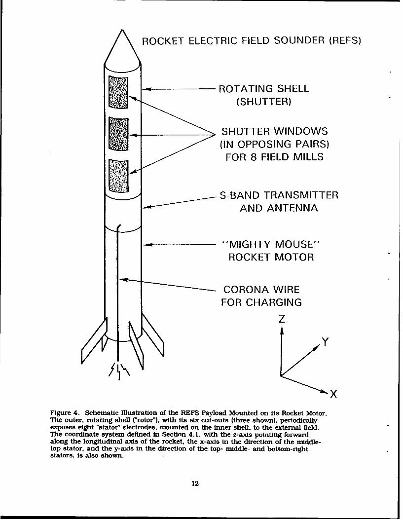
The most important innovation in the NMIMT proposal was the use of a single, long,cylindrical shell concentric with, and rotating about, the longitudinal axis of the rocket. Thisshell covers most of the payload and acts as the "rotor" for all the mills, as shown in Figure 4.With this design concept, the number of mills can be increased simply by gluing additional

24 Kositsky, J., K.L. Glori, RA. Mafflone, D.H. Cronin, J.E. Nanevicz and R. Harris-Hobbs,(1991) Airborne Field Mill (ABFM) System Calibration Report, Project 1449, SRI International,Menlo Park, CA.

25 Jones, J.J., (1990) Electric charge acquired by airplanes penetrating thunderstorms,J. Geophys. Res., 95:16,589-16,600.

26 Bailey, J.C., and R.V. Anderson, (1987) Experimental Calibration of a Vector Electric lMeldMeter Measurement System on an Aircraft," Memorandum Report 5900, Naval ResearchLaboratory, Washington, DC.27 Laroche, P., (1986) Airborne measurements of electrical atmospheric field produced by

convective clouds, Rev. Phys. AppL, 21:809-815.

11

ROCKET ELECTRIC FIELD SOUNDER (REFS)

ROTATING SHELL

W (SHUTTER)

SHUTTER WINDOWS(IN OPPOSING PAIRS)

FOR 8 FIELD MILLS

L S-BAND TRANSMITTERAND ANTENNA

"MIGHTY MOUSE"ROCKET MOTOR

CORONA WIRE

FOR CHARGING

z

Figure 4. Schematic Illustration of the REFS Payload Mounted on its Rocket Motor.The outer, rotating shell ("rotor"), with its six cut-outs (three shown), periodicallyexposes eight "stator" electrodes, mounted on the inner shell, to the external field.The coordinate system defined In Section 4.1, with the z-axis pointing forwardalong the longitudinal axis of the rocket, the x-axis in the direction of the middle-top stator, and the y-axis in the direction of the top- middle- and bottom-rightstators, Is also shown.

12

"stator" electrodes onto the payload body and cutting corresponding holes in the rotor to chop

the field to these stators.

In consideration of the low cost of adding sensors to the payload, it was decided to use a

total of eight field mills on REFS. arranged in symmetrical pairs on opposite sides of thelongitudinal axis (see Figure 4). These pairs are located at three different longitudinal

positions: one near the forward end, one near the aft end (near the center of the vehicle,

accounting for the motor), and two in the middle of the payload. One of the middle pairs has

an azimuthal orientation perpendicular to that of the other three, allowing both transverse

field components to be measured. This approach takes maximum advantage of the cylindricalsymmetry. Opposing mill signals can be differenced to cancel vehicle charge and longitudinal

field (giving three independent measurements of one transverse component and one

measurement of the other) and can be summed to cancel transverse field (giving three

independent quantities -- one redundantly -- from which to derive longitudinal field andvehicle charge). Furthermore, all eight stators can be covered and uncovered twice per

revolution of the rotor by only three symmetrical pairs of opposing holes.

The considerable redundancy afforded by these eight mills allows the data to be checked

against the electrostatic model of the rocket (see Section 6. 1) for possible inconsistencies

caused by the exhaust plume, space charge in the immediate vicinity of the vehicle, or spuriousreadings from individual mills. A good fit of model to data indicates proper functioning of the

payload and, hence, reliah!e derived values for the ambient field components. These

components can still be derived redundantly with as many as three bad mills, as long as the

malfunctioning sensors are not grouped in an unfortunate way.

As with any other ABFM system, REFS must have the capability to charge itself artificially

in flight. The NMIMT proposal called for an on-board, high-voltage power supply to energize acorona emitter that dumps ions into the air stream, periodically charging the vehicle to

moderate potentials. It was considered possible that a single-polarity supply might rapidlydrive the rocket to its corona threshold and be unable to significantly change its potential

thereafter. Therefore, a dual-polarity supply was necessary, at least for the first flight, toguarantee a known charging cycle. Measurement of the voltage on the corona emitter as a

function of time was also required. Such a cycle allows the self-charge coefficients of the

various mills to be determined very accurately, enabling precise measurement of the ambient

field regardless of vehicle charge. As an additional benefit, artificial charging provides a

functional check and relative calibration of all the mills in flight.

Another valuable check is provided by telemetering the entire waveform from each mill(charge on the stator as a function of time) back to the ground, rather than performing the

synchronous rectification on board. In this case, rotor-position information must also betelemetered. NMIMT suggested the use of passive optical detectors looking at the sky through a

series of holes in the rotor. Since the entire vehicle rotates throughout the flight, constancy of

the ambient light level can be used as an indicator of cloud penetration. Although this low-

level approach to the signal processing requires a much wider telemetry bandwidth than theconventional one, it enables most potential malfunctions of the mills to be positively

diagnosed, and it significantly reduces the size of the electronics package.

13

With simple glued-on stator plates, it is not practical to electrically shield the statorinsulators from the shutter -- a common practice to minimize spurious signals in shutter fieldmills due to surface charge on these insulators. A refinement of the design has beenintroduced to solve this problem. Each hole in the rotor is made smaller than the

corresponding stator plate. Thus, there are time intervals both when the stator is fully covered

and when a constant area of stator is exposed. During these two intervals the insulators

surrounding the stators, and stator edges themselves, are fully covered by the rotor, so that anyeffects of charge on the insulators are the same. Averaging the mill signal over each of these

intervals and differencing the results accomplishes the synchronous rectification while

canceling any contribution from surface charge.

Three more sensors have been added to define vehicle performance. A pressure transducer

is used to determine altitude. The critical information here is the apogee time and height,from which the rest of the trajectory can be estimated with computer models. The ignition

time and duration of motor burn are monitored by a longitudinal accelerometer. Finally, therotation of the vehicle is defined with a single-axis magnetometer oriented transverse to the

rocket axis. This completes the overall conceptual design.

3. ELECTRONIC DESIGN

This section includes descriptions of the REFS block diagram, electronics, Ground Support

Equipment (GSE) and internal/external power-switching circuits. These circuits were

originally designed by NMIMT, but were modified and improved by the Aerospace Engineering

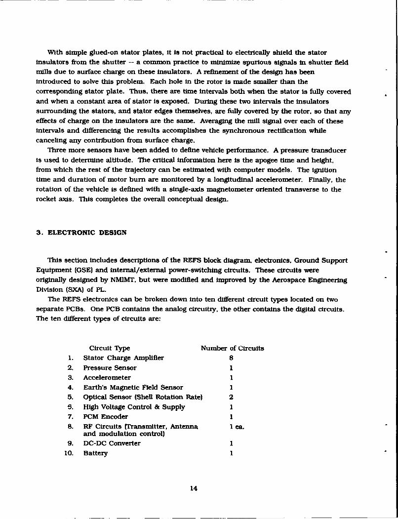
Division (SXA) of PL.The REFS electronics can be broken down into ten different circuit types located on two

separate PCBs. One PCB contains the analog circuitry, the other contains the digital circuits.

The ten different types of circuits are:

Circuit Type Number of Circuits

1. Stator Charge Amplifier 8

2. Pressure Sensor 1

3. Accelerometer 1

4. Earth's Magnetic Field Sensor 1

5. Optical Sensor (Shell Rotation Rate) 2

5. High Voltage Control & Supply 1

7. PCM Encoder 1

8. RF Circuits (Transmitter, Antenna 1 ea.and modulation control)

9. DC-DC Converter 1

10. Battery 1

14

See the block diagram (Figure 5) for more detail.

3.1 Stator Charge Amplifier (Figure 6)

There is one Stator Charge Amplifier (SCA) for each field-mill stator located on the REFSpay,,ad. Each SCA is identical and contains three stages; a charge amplifier with lightning

protection, a filter, and a current driver.

Two diodes in opposite orientations provide protection in the event of a nearby lightning

strike. If the input of the charge amplifier is forced above or below "virtual" ground by more

than 0.5 V. then these diodes will conduct and protect the amplifier. IUghtning-protectiondiodes are placed on the inputs of all REFS analog circuits.

The charge amplifier provides a voltage output that is proportional to the electric field seen

by the stator plate. When the shutter opens, the 0.01 1F capacitor in the feedback loop of the

first operational amplifier (opamp) charges up to a voltage that is proportional to the charge

induced on the stator by the electric field incident upon it. The 33 MOhm resistor in the

feedback loop is there to provide bias current for the opamp. The resistor and capacitor pair

must have a time constant sufficiently large so as not to discharge the capacitor significantly

before the shutter is open again. The rotating shell openings have a period of 0.033 s. The33 MOhm resistor provides a time constant of 0.33 s. This is sufficient to provide the bias

current without compromising the measurement.The second stage of this circuit is a low-pass filter. This filter will be discussed here, but it

appears in all the other analog circuits. This filter has a gain of 1.26 and a cutoff frequency of

1 kHz. It is constructed using one LF444 and two 1000 pF capacitors that provide two poles.This configuration is usually called a Sallen/Key filter. It is used for removing high frequency

noise from its channel. The filter is followed by a current driver with unity gain.The sensitivity of the stator circuitry was set to provide a full-scale output in a field of 1

MV/m. This was done by setting the feedback capacitor Cf in the first stage of the charge

amplifier. The smaller this capacitor, the more sensitive the amplifier. The capacitor waschosen according to the formula Vut = Q/Cp, where Vout is the output of the first stage of the

charge amplifier, and Q is the charge induced on the stator plate. This charge is related to the

field as discussed in Section 6.The signal-to-noise ratio (S/N) of this circuit is calculated by taking the full-scale output

range, corresponding to 1 MV/m, and dividing it by the noise level. The S/N for all of the

stator channels was about 50 dB.

3.2 Pressure Sensor (Figure 7)

The pressure transducer was used to ascertain payload altitude, more specifically themoment and height of apogee. The circuitry centers on an SCX15AN pressure transducer made

by Sensyn. Irc. This absolute pressure transducer is a bridge device with a range of0 to 15 PSI. It produces a change in bridge resistance that is proportional to pressure.

15

U00

x0 a r

- 1S

h

4.

� IS �KI. S

S�

�: IN Uif S 4 -

I? op. g

.- K 0

K S II K S3

4S0 K

no * o

Ku AK -40 no 0

K K- K - K -

0* �K p4* CKen *44 on nitKb K. K. 0.4

- � -w-Oq

U�I!�. p.: -

00 *0 I*0 40

O Ka. * n * (j)* 0 4.' - K -

K K* K - K K- 0 4t 0 0K .' K -

3

S -4. U. V.2

K-n

.4- S - UK.

K. S. K...

U.. U., K "U.4Kb

OhS h

-K -K 'SN:0- -

p. p. 4..U

-R 3On 0..

Ks UK

K.. p.0 K.. VtC

Un

S

17

14.

u . 00

. .3

it.S

IleL

uo

F-0

18

When powered by a +10 V supply voltage, this unit produces an output of 6 mV/PSI. The output

of this device goes into an instrumentation amplifier and low-pass filter. The gain term forthis Instrumentation amplifier can be expressed as Vout a 18.2 JVpp - 1.055 VpmJ, where Vpp Isthe positive output of the device and Vpm ts the negative output. The low-pass filter has been

discussed In Section 3. 1.The error due to noise in this circuit is calculated by taking the noise level in volts and

translating it to a corresponding altitude error. The noise level of 10 mV corresponds to analtitude error of about 180 ft.

Calibration was performed In the SXA vacuum chamber at the Phillips Laboratory.Figure 8 shows the result.

3.3 Accelerometer (Figure 9)

The longitudinal accelerometer was intended to provide the experimenter with the exact

times of liftoff and motor burnout. The principal device used in the accelerometer circuit isthe SXL200G, again made by Sensym, Inc. This accelerometer is of the bridge variety andproduces a voltage output that is proportional to acceleration. The typical output Is 200 AV/g.The output of this device is run into an instrumentation amplifier with a gain term of Vut =

170[Vam - 1.006 VapJ, where Vap is the positive output of the device and Va Is the negative

output. The signal Is then run through the low-pass filter discussed in Section 3. 1.The error due to noise in this circuit is calculated by taking the noise level In volts and

translating It to a corresponding acceleration error. The noise level of 10 mV translates to anerror in acceleration of about 0.23 g.

Shock testing was used to calibrate the accelerometer. An 11.49 ms, half-sine shock pulsewas applied to the base of the payload as part of environmental testing. It appeared duringthis test that the accelerometer was functioning properly and that its range was well withinthe limits that the payload was expected to see during flight. During the burn phase of theflight, however, the accelerometer saturated. It became obvious that the calibration techniqueused was insufficient. One probable cause for the error is that the internal structure dampedthe shock transmitted to the accelerometer (the sensor Is mounted on the electronics boards).Therefore, 11.49 ms was too short a duration.

3.4 Magnetic Field Sensor (Figure 10)

The magnetic-field-sensing circuitry was designed to provide an uncalibrated measure ofthe transverse component of the ambient magnetic field. Through this circuitry, theorientation of the payload with respect to Earth's magnetic field can be estimated. Inparticular, payload rotation rate can be determined. The sensor used is a SAS231W made bySiemens, Inc. This sensor measures magnetic flux density and has a sensitivity of 100mV/mT. Flux concentrators made of Mu-Metal were added on the top and bottom of the sensor

19

PRESSURE XDUCER CALIBRATIONboard set #1

-----------L=---------.L.-. ---- -- ----- L-------

-08----------- -------- -- ----- - - - - - - - - - -

----- ----------------------- ------I------I------*---- --------------------

08-

PRESSURE~psi)

Figure 8. Calibration of the Pressure Transducer in PL/SXA Environmental Chamber

to bring Earth's magnetic field up to a level where the SAS231W could sense It. An amplifierwith a gain of 22 was used to bring the output of the SAS231W to a scale of 0.6 V peak to peak.Because of the large temperature sensitivity of this sensor, the circuit showed a severe driftwith temperature. It was necessary to add resistors R15B and R16B to force the circuit tooperate over the appropriate temperature range.

Calibration was unnecessary for this circuit. S/N is calculated by dividing the signal level(0.6 V) by the noise (.01 V), giving 36 dB.

20

2 2

:� ;�: U

g 2.4. - 0

*ft * 3I�2. *

h�I� �

�gu ., 4-'

U. Mi

43.4.U.

Ii3-

-a I4'

III

a I

21

ama

am

LI --

j"II4 aa

00a

AC.9

all I..

soC

am4

22~gt

3.5 Optical Sensors (Figure 11)

Two optical sensors were developed to provide unambiguous data on the rotor position andto indicate when the payload penetrated a cloud. Each optical sensor looks outward through ahole in the inner shell of the payload. Light can reach the first sensor through a series of 16evenly spaced holes in the outer (rotating) shell. The second optical sensor is illuminated only

by a single hole aligned with the rotor cutouts. (See Section 4.2 for further description of themechanical configuration of these sensors.) The first sensor provides rotor angular velocity.

the second provides absolute angular position. The use of ambient light allows the sky/earthrelative brightness to be monitored as the payload rotates. Because light intensity is nearly

isotropic within a cloud, but seldom so outside one, it was expected to detect cloud penetrationswith these sensors, independent of vehicle charging.

Each optical sensor is supported by an identical circuit. EG&G photodiodes are used toproduce a voltage that Is proportional to incident light. This voltage is applied to an amplifier

with a gain of 7.67 and then into the low pass filter discussed earlier. Resistors R13X throughR16X were added to provide a 0.298 V offset to center the two signals.

The signal difference between the covered and the uncovered state for these sensors wastypically about 1 V in hazy sunshine. S/N was calculated by dividing this signal (1 V) by the

noise (0.01 V), giving 40 dB.

3.6 High Voltage Supply and Control (Figure 12)

As explained in Section 2.2, two high-voltage power supplies were included in the payload.These supplies, plus and minus 10,000 V, respectively, were alternately connected through aresistor to a trailing corona wire for 0.1 s out of every 1.6 s. Provisions were also made to

monitor the voltage on the corona wire during flight.The original NMIMT design called for four control signals to be generated by a

Programmable Logic Device (PLD). The first two applied power to the high-voltage supplies at

different times. This reduced the duty cycle on the supplies, saving battery power. The thirdcontrolled a high-voltage relay to switch between the plus and minus supplies. The fourthdrove another high-voltage relay to connect the voltage to the corona wire. These PLD outputswere connected to the gates of MOSFETS that applied power to the supplies and relays.

Soon after testing of the electronics began, three significant problems arose. First, whenhigh voltage was applied to the relays, the PLDs would enter an unstable state that changed thecircuit timing. This state could only be reset by cycling power. Second, the MOSFET driverswere constantly being "blown" by spikes induced on the power lines when the high-voltagerelays switched. Third, a telemetry dropout of approximately 10 ms was induced every time ahigh-voltage relay was switched.

23

- - -

o 1.

t•f. £ --

N.. IMO

-IN -O -

ft. f2 0

ii"

i.i

25 i!SI

f ! N =

After many hours spent in trying to isolate the high-voltage electronics from the control

electronics, we decided to replace the PLDs with conventional CMOS circuitry. This CMOS

circuitry consisted of a binary counter (54HC4020), three 3-input NAND gates and one 4-input

AND gate. These three chips were used to generate VI, V2, VN and VP. This solution proved

effective in preventing the erroneous timing state from occurring. To make the driving

electronics less susceptible to high-voltage spikes, the MOSFETS were also replaced with

standard NPN transistors that did not 'blow" during high-voltage switching.

The original electronics design provided to the Air Force included no isolation between the

high voltage system and the telemetry system. This lack of isolation caused dropouts to

appear on the data channels whenever the high voltage was switched. Because of schedule andcost constraints, it was impossible to redesign the payload to add this isolation. Every effort

was made to reduce these dropouts through the use of varistors and bypass capacitors, but itwas impossible to remove them completely. The payload was flown with telemetry dropouts

that were short enough to be considered bearable.The voltage on the corona wire was monitored through an amplifier with a gain of

0.000258. Because of the series resistor R7B, however, this voltage was only R,/(2Rc + 250xi06)

times that developed by the high-voltage supplies, where R, is the "effective" resistance of the

corona point. Thus, a maximum of around 5 kV could be applied to the corona point. The

signal was again filtered, as d! ,.uised earlier.

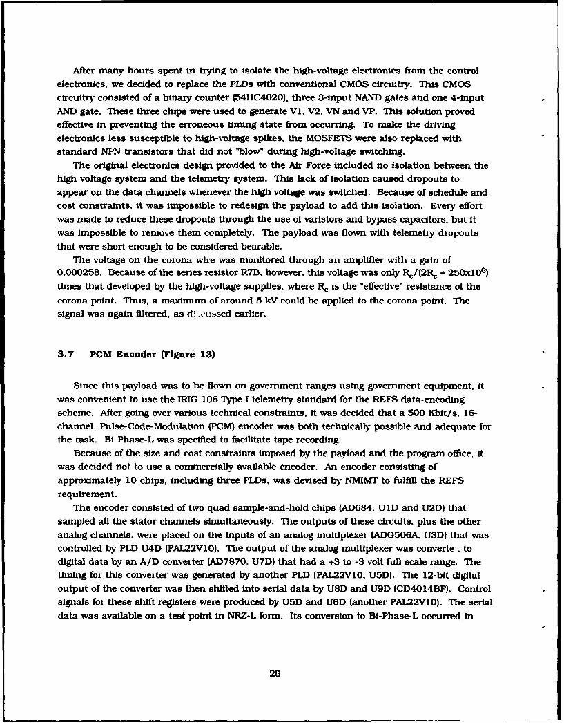
3.7 PCM Encoder (Figure 13)

Since this payload was to be flown on government ranges using government equipment, itwas convenient to use the IRIG 106 Type I telemetry standard for the REFS data-encoding

scheme. After going over various technical constraints, it was decided that a 500 Kbit/s, 16-

channel, Pulse-Code-Modulation (PCM) encoder was both technically possible and adequate for

the task. Bi-Phase-L was specified to facilitate tape recording.

Because of the size and cost constraints imposed by the payload and the program office, it

was decided not to use a commercially available encoder. An encoder consisting of

approximately 10 chips, including three PLDs, was devised by NMIMT to fulfill the REFS

requirement.

The encoder consisted of two quad sample-and-hold chips (AD684, UID and U2D) that

sampled all the stator channels simultaneously. The outputs of these circuits, plus the other

analog channels, were placed on the inputs of an analog multiplexer (ADG506A, U3D) that was

controlled by PLD U4D (PAL22VIO). The output of the analog multiplexer was converte-, to

digital data by an A/D converter (AD7870, U7D) that had a +3 to -3 volt full scale range. Thetiming for this converter was generated by another PLD (PAL22VIO, U5D). The 12-bit digital

output of the converter was then shifted into serial data by U8D and U9D (CD4014BF). Control

signals for these shift registers were produced by U5D and U6D (another PAL22VIO). The serial

data was available on a test point in NRZ-L form. Its conversion to Bi-Phase-L occurred in

26

II

P WU~O u.

0.

A 00 an3

DC:

0000 00

IaF- I

27a

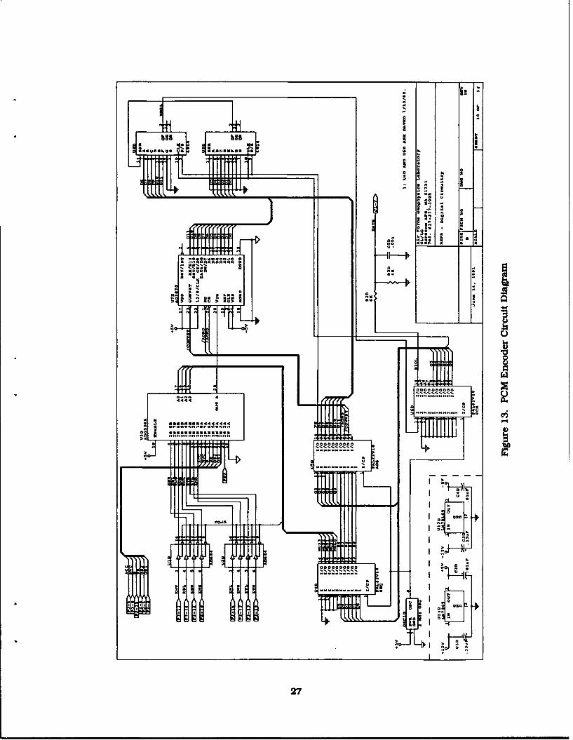
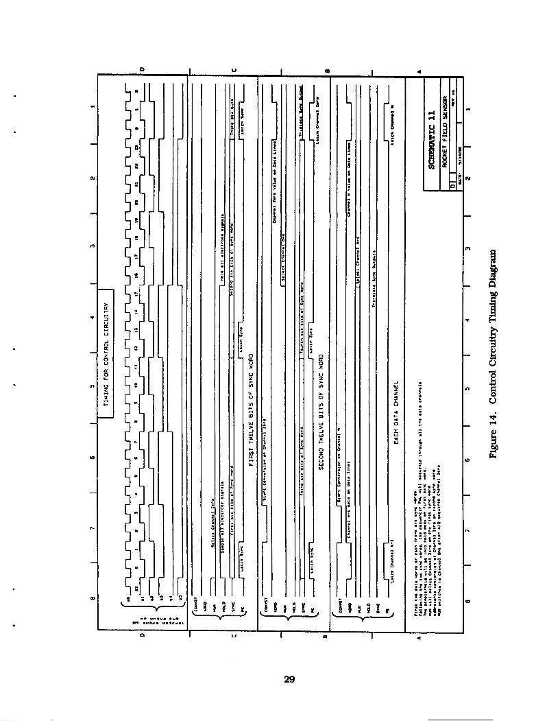
U6D. The whole system ran off a 2 Mhz oscillator and intermediate timing signals generatedby U4D. For a detailed timing diagram see Figure 14.

3.8 RF System

Due to the small size and high acceleration of the REFS vehicle, the only transmitteravailable "off the sheW was a ballistic, Phase-Modulated (PM), S-band transmitter, modelT4XO-S, manufactured by Microcom, Inc. This transmitter was approximately 1.7 inches indiameter and was specified at 1000 g acceleration. It had a center frequency of 2235.5 Mhz anda minimum output power of 0.200 W. Table 1 shows range calculations for the REFS flight.

As previously stated, the T4XO-S is phase modulated. This type of modulation is nottypically used for sounding-rocket telemetry. To standardize, it was necessary to convert our

PM signal to a Frequency Modulated (FM) signal. A pre-modulation integrator network alsoshown in Figure 13 was placed between the output of the PCM encoder and the transmitter tomake the output appear to be FM.

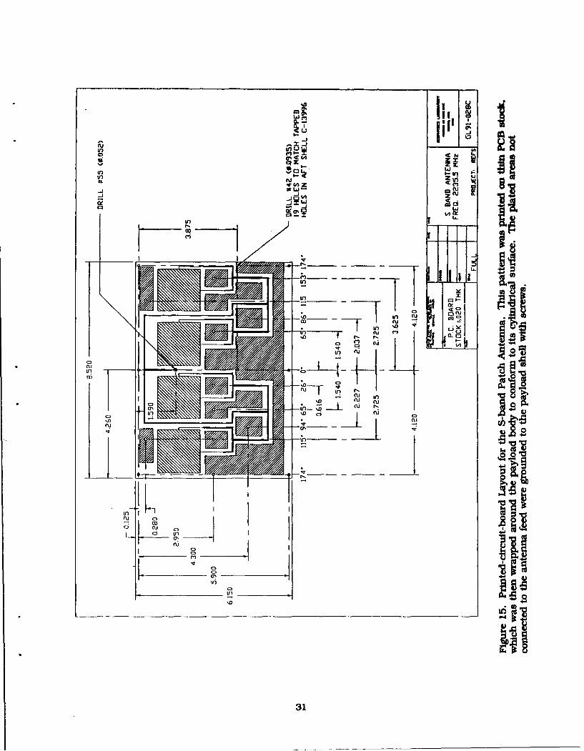
The telemetry antenna was required to conform to the cylindrical shape of the payloadwith no protrusions and to radiate a signal at 2235.5 Mhz that was Independent of rocketrotation. It was developed for REFS by Rome Air Development Center (RADC) and consisted offour square patches that were each fed through impedance transformers on two sides 90 degapart (see Figure 15). The antenna was printed on flexible printed-circuit board made of0.015-in thick PTFE (dielectric constant 2.2) clad with copper on both sides, which waswrapped around the payload and epoxied in place. Unused portions of the antenna surfacewere left plated and were grounded to the shell by screws to reduce insulating surface area.

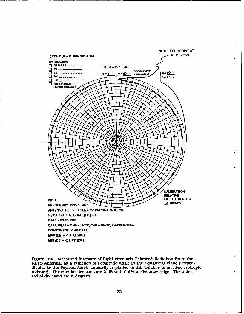
The Physical Science Laboratory at New Mexico State University measured the radiationpattern of the REFS antenna in flight configuration. As expected, radiation from the antenna

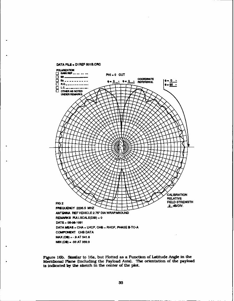
was strongly right-hand-circularly polarized, left-circular power being more than 11 dBweaker overall. The right-circular radiation pattern was very uniform with longitude angle, asillustrated in Figuire 16a. Narrow transmission nulls were apparent out of the fore and aft

ends of the payload, as shown in Figure 16b. The radiated power was -2.97 dBl (normalized toan Ideal spherical radiator) and the angular coverage at -10 dBl was 99.7 percent of the sphere.

28

a U I

- I -

ccp4

* acc o -

u3ioCc5 - i

I-

U- I

0 ai

- 0 0 -9

> >qLi -

tLi w a4c C

00

o t

3 3C

o, 1i L

-zso -~ *

Cf hz z cis. is. 0

3 0 0 4

in I a C4

U La

29 4

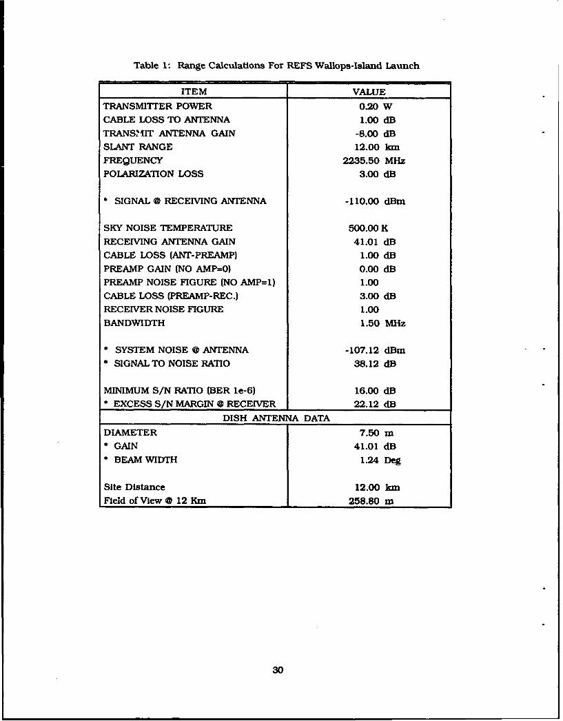
Table 1: Range Calculations For REFS Wallops-Island Launch

ITEM VALUE

TRANSMrITER POWER 0.20 W

CABLE LOSS TO ANTENNA 1.00 dBTRANSMIT ANTENNA GAIN -8.00 dB

SLANT RANGE 12.00 km

FREQUENCY 2235.50 MHzPOLARIZATION LOSS 3.00 dB

* SIGNAL @ RECEIVING ANTENNA -110.00 dBm

SKY NOISE TEMPERATURE 500.00 K

RECEIVING ANTENNA GAIN 41.01 dB

CABLE LOSS (ANT-PREAMP) 1.00 dB

PREAMP GAIN (NO AMP=0) 0.00 dBPREAMP NOISE FIGURE (NO AMP=l) 1.00

CABLE LOSS (PREAMP-REC.) 3.00 dBRECEIVER NOISE FIGURE 1.00

BANDWIDTH 1.50 MHz

SYSTEM NOISE @ ANTENNA -107.12 dBm

* SIGNAL TO NOISE RATIO 38.12 dB

MINIMUM S/N RATIO (BER le-6) 16.00 dB

* EXCESS S/N MARGIN @ RECEIVER 22.12 dB

DISH ANTENNA DATA

DIAMETER 7.50 m

GAIN 41.01 dB

* BEAM WIDTH 1.24 Deg

Site Distance 12.00 km

Field of View 0 12 Km 258.80 m

30

M IN

inn

LOL.

tw, CU

Cu c

ixinl31D

NOTE: FEED POINT AT

DATA FILE = D1 REF S01B.CRC *=0. e=90

A GAIN REF VEHIE THETA 290.1 CUT] E9 COORDINAT * =90 •

0 R.C -------------- 0=9 .=gEl L.C.- -- -- --El OTHER AS NOTED

UNDER REMARKS.

CALIBRATIONRELATIVE

FIG I FIELD STRENGTH

FREQUENCY 2235.5 MHZ _?._dB/D|V.

ANTENNA REF VEHICLE 2.75" DIA WRAPAROUND

REMARKS FULLSCALE(DBI) - 0

DATE = 05-08-1991

DATA MEAS a CHA - LHCP, CHB - RHOP, PHASE B-TO-ACOMPONENT CHB DATA

MAX (DB) - -1.4 AT 280.1

MIN (DB) = -2.8 AT 228.2

Figure 16a. Measured Intensity of Right-circularly Polarized Radiation From theREFS Antenna, as a Function of Longitude Angle in the Equatorial Plane (Perpen-dicular to the Payload Axis). Intensity is plotted in dBI (relative to an Ideal Isotropicradiator). The circular divisions are 2 dB with 0 dBi at the outer edge. The outerradial divisions are 5 degrees.

32

DATA FLU.a DI REF 601 B.CR1C

E] amNREF .. .. PHI 0 CUT

A0 U E REF VEHICLE---- 2.7' IAWRA AR UN

DAT 0--- -- ---i 9910D3ATAE ~AS NWH =LC, H RC. HSEBT-

COMPONEATIBRATDAT

RMAXS (O) = -.9 AT 341.8

MI6N(DO) -- 33 AT 359.9

Figure 16b. Sinmilar to 16a, but Plotted as a Function of Latitude Angle in theMeridional Plan (Including the Payload Axids). T1e orientation of the payloadis indicated bys the sketch in the center of the plot.

33

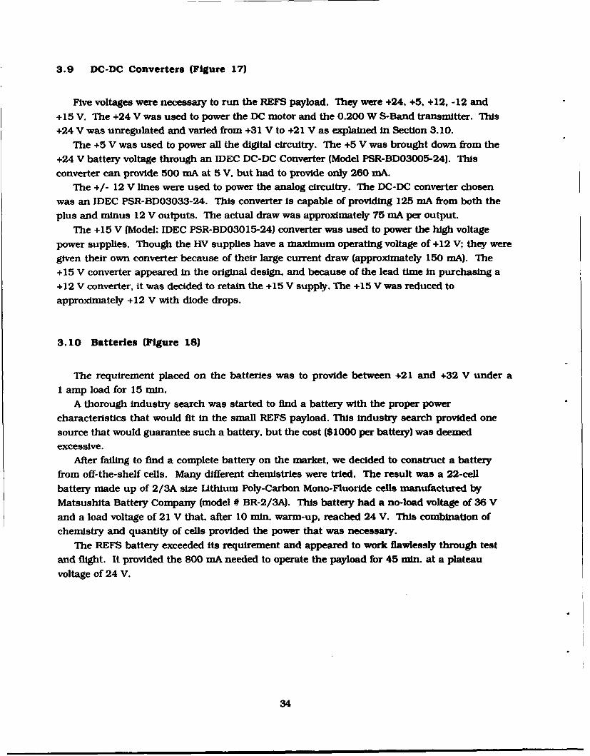
3.9 DC-DC Converters (Figure 17)

Five voltages were necessary to run the REFS payload. They were +24, +5, +12, -12 and

+ 15 V. The +24 V was used to power the DC motor and the 0.200 W S-Band transmitter. This

+24 V was unregulated and varied from +31 V to +21 V as explained in Section 3.10.

The +5 V was used to power all the digital circuitry. The +5 V was brought down from the

+24 V battery voltage through an IDEC DC-DC Converter (Model PSR-BD03005-24). This

converter can provide 500 mA at 5 V, but had to provide only 260 mA.

The +/- 12 V lines were used to power the analog circuitry. The DC-DC converter chosen

was an IDEC PSR-BD03033-24. This converter is capable of providing 125 mA from both the

plus and minus 12 V outputs. The actual draw was approximately 75 mA per output.

The +15 V (Model: IDEC PSR-BD03015-24) converter was used to power the high voltage

power supplies. Though the HV supplies have a maximum operating voltage of +12 V; they were

given their own converter because of their large current draw (approximately 150 mA). The

+ 15 V converter appeared in the original design, and because of the lead time in purchasing a

+12 V converter, it was decided to retain the +15 V supply. The +15 V was reduced to

approximately +12 V with diode drops.

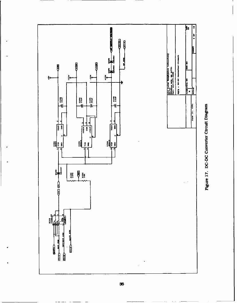
3.10 Batteries (Figure 18)

The requirement placed on the batteries was to provide between +21 and +32 V under a

1 amp load for 15 min.

A thorough industry search was started to find a battery with the proper power

characteristics that would fit in the small REFS payload. This industry search provided one

source that would guarantee such a battery, but the cost ($1000 per battery) was deemed

excessive.

After failing to find a complete battery on the market, we decided to construct a battery

from off-the-shelf cells. Many different chemistries were tried. The result was a 22-cell

battery made up of 2/3A size Lithium Poly-Carbon Mono-Fluoride cells manufactured by

Matsushita Battery Company (model # BR-2/3A). This battery had a no-load voltage of 36 V

and a load voltage of 21 V that, after 10 min. warm-up, reached 24 V. This combination of

chemistry and quantity of cells provided the power that was necessary.

The REFS battery exceeded its requirement and appeared to work flawlessly through test

and flight. It provided the 800 mA needed to operate the payload for 45 min. at a plateau

voltage of 24 V.

34

I I

I IUU I_-•. !: '=.I

353

0

hi 4

W64 r- 4,.4 C

me 0 ) 0 Is-U . .94 W,.,... K S, .-

we QUO 0 a u00 ,-- ., 1 .4 a0-1.- 0-4" if m m ,-4

IL OAW Ks- aS. I AZZ W 6. -C , I o*41 wi0494 1. U. I.4 -. 0o. a .4.) -&a 44 S U #aTTW TT - * -,

S ii "L

a aALI

u Z

0a* 0

4-

am

.... .. ...........................................................................

to

i 441L0

z

364

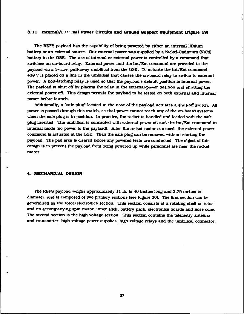
8.11 Internal/I Y nal Power Circuits and Ground Support Equipment (Figure 19)

The REFS payload has the capability of being powered by either an internal lithiumbattery or an external source. Our external power was supplied by a Nickel-Cadmium (NiCd)battery in the GSE. The use of internal or external power is controlled by a command thatswitches an on-board relay. External power and the Int/Ext command are provided to thepayload via a 3-wire, pull-away umbilical from the GSE. To actuate the Int/Ext command.+28 V is placed on a line in the umbilical that causes the on-board relay to switch to externalpower. A non-latching relay Is used so that the payload's default position Is internal power.The payload is shut off by placing the relay In the external-power position and shutting theexternal power off. This design permits the payload to be tested on both external and internal

power before launch.Additionally, a "safe plug" located in the nose of the payload actuates a shut-off switch. All

power is passed through this switch, so that power cannot reach any of the on-board systemswhen the safe plug Is in position. In practice, the rocket Is handled and loaded with the safeplug inserted. The umbilical is connected with external power off and the Int/Ext command ininternal mode (no power to the payload). After the rocket motor is armed, the external-powercommand Is actuated at the GSE. Then the safe plug can be removed without starting thepayload. The pad area is cleared before any powered tests are conducted. The object of thisdesign Is to prevent the payload from being powered up while personnel are near the rocketmotor.

4. MECHANICAL DESIGN

The REFS payload weighs approximately 11 lb, is 40 inches long and 2.75 inches indiameter, and is composed of two primary sections (see Figure 20). The first section can begeneralized as the rotor/electronics section. This section consists of a rotating shell or rotorand its accompanying spin motor, inner shell, battery pack, electronics boards and nose cone.The second section is the high voltage section. This section contains the telemetry antennaand transmitter, high voltage power supplies, high voltage relays and the umbilical connector.

37

)

L4.

Q

UI

*1.1 U

�

�*� -. 0

.� �c *�� ao *0

Ia.LS �

* U

* 3* ILQU NC

.5 3* L�C '�

U 3J �U0.

Id . -U KIi. 4..4

IdWIR g C.)

11~

-- -------I 1\ \\ 3

4.1 Rocket Motor

The REFS payload was designed for launch aboard a 2.75-in. Folding Fin Aircraft Rocket

(FFAR. also known as "Mighty Mouse"). This motor is 2.75 inches in diameter and 39 inches

long, as measured from the end of the fins (folded) to the motor head cap. The motor was first

produced in 1953 and has gone though many upgrades and revisions. Although originally

designed for launch from aircraft, these motors have been fired from ground-based launchers

by the NASA Wallops Flight Facility (WFF) since 1962 as a radar test rocket. The FFAR has

also been used by many other organizations, including the Naval Ordnance Lab, the NASA

Langley Research Center, and the Atlantic Research Corporation. The FFAR was chosen as the

motor for REFS because it is inexpensive and readily available.

The type of FFAR used in support of this launch was the Mark 40, Mod 4. This rocket

produces approximately 734 lbf of thrust for 1.55 seconds. The total impulse Is rated at 1170lbf-sec. The FFAR uses a single motor with 4 exhaust nozzles. The nozzle ends are cut at an

angle, forming a "scarfed" edge. This scarfing causes the thrust vector from each nozzle to beslightly misaligned. This intentional thrust misalignment spins the rocket, instead of the fin

misalignment more commonly used. The spin helps to stabilize the vehicle, and also reduces

errors caused by inadvertent thrust misalignment.

The FFAR incorporates a set of four, symmetrically aligned, folding fins. The fins are

deployed by a plunger actuator located between the nozzles. Chamber pressure during the burnphase forces the plunger out, thereby deploying the fins as soon as the rocket leaves its launch

tube.For REFS the motor was slightly modified by the addition of eight teflon bumpers glued to

Its sides at the top and bottom ends. These bumpers made a snug fit in the modified launch

tube (see Section 4.4) while protecting the trailing corona wire from abrasion.

4.2 Rotor/Electronics Section

This section deals with the rotor/electronics section of the payload. As a point of referencein this discussion, the nose cone is considered to be forward and the rocket motor is

considered to be located aft. This coordinate system applies to the entire payload. For

simplicity, efforts are made to explain the payload starting from the nose cone and moving aft.

The nose cone (see Figure 21) is constructed of 6061 aluminum. It is approximately 5.5

inches long and 2.75 inches at the base, forming a 30 degree cone. The tip of the cone is not

sharp but is blunted with a 0.187-inch radius. The interior is hollow to allow space for theouter shell spin motor. The payload safe/arm switch is also incorporated into the nose cone.

The nose cone is attached to the inner shell using 6-32 pan head screws.

The rotor (rotating outer shell) spin-motor assembly is housed under the nose cone (see

Figures 22 and 23). It consists of a 24 V DC motor, Idler gear, drive gear, and mounting

40

Of

3WJ w

Ii 0

zz

V -

IR-A

41

b

C)

°aCU)

0U0

0 3

cC>•C)

0I

U-U

42CL

OA , 1j I O

a. d o LB

-jI a1 t E

LlEw

i3 0, aFT

~~'IZL I r

4~IX

43

bracket. The spin motor drives the rotor through the idle and drive gears. The drive gear ismounted to the motor and has 36 teeth. Power Is transferred through the Idler gear to a 140-tooth gear mounted on the rotor. This results in a speed reduction of 3.89 to 1 and provides 15rps (900 rpm) to the rotor under no load. At maximum rocket velocity of about 560 m/s, this

corresponds to one rotation (or two field readings) every 37 m of flight.

The rotor (see Figures 20 and 24) is a hollow aluminum cylinder 28 Inches long, 2.75 inchesin diameter, and 0.063 inches in wall thickness. For simplicity, a stock, "off-the-shelf' tubingwas used for the rotor. This shell rotates on two bearings. The forward bearing Is mounted to

the rotor (see Figure 25), while the aft bearing is mounted to the mid joint (see Figure 26) sothat the shell slides over it. The bearings are lubricated by an electrically conductingmolybdenum disulfide grease to assure that the shell remains at ground potential. The shell isrotated by the spin motor assembly described previously, through a gear mounted to the inside

diameter of the rotor.

Six "windows" or openings are present in the rotor. Each window Is approximately 4inches long (measured along cylinder) and 45 degrees of arc length wide. The windows arelocated in pairs, the members of each pair being 180 degrees apart (on opposite sides of therotor). One pair is located near the forward end of the shell, the second pair is near the mid

point, and the third is near the aft end. The purpose for the windows and rotation of the outershell is to provide a "shutter" for the stators mounted on the inner shell, an essentialrequirement for proper operation of the field mills.

The rotation rate and position of the rotor are measured using optical sensors(photodlodes) located on the electronic boards, as described in Section 3.5. A series of sixteen0.158 Inch diameter holes is drilled in the rotor. The holes are equally spacedcircumferentially around the rotor and are located between the forward and middle windows(see Figure 24, Sta. 12.875). A single 0.158-inch diameter hole is located 0.3 inch below theseries of 16 (Figure 24, Sta. 13.175).

The inner shell (see Figures 20 and 27) is the support structure for the nose cone, spinmotor, electronics boards, battery pack, and rotor. It is constructed of "stock" aluminumtubing, is approximately 26.7 inches long, 2.375 inches in diameter, and has a wall thicknessof 0.058 inch. A total of 8 stators Is mounted to the outside of the shell using a high strengthepoxy. The stators are copper rectangles with an insulating backing and borders. Each stator

Is approximately 5.5 inches long and 1.85 inches wide, including a 3 mm insulating border onall sides. The stators are arranged In opposing pairs (that is, 180 degrees apart). Two statorsare mounted near the forward (nose-cone) end of the inner shell, four stators are mounted nearthe middle, and the last pair is mounted near the aft (mid-joint) end. Of the four sets of

stators, three pairs are arranged in line, while the fourth pair is located at the samelongitudinal position as the middle pair, but rotated 90 degrees.

The stator material Itself is a PTFE core sandwiched between thin copper sheeting,resembling a raw printed-circuit board. This Is the same material used for the telemetry

antenna described in Section 3.8. This material is quite pliable and capable of being bent toconform to the curvature of the inner shell. The stators are constructed using conventional

PCB fabrication techniques.

44

IINJHsi

lagHi I

45

46

0

0I

47

lil

Vol ii

aa

aSea

LIJLi

48

The battery pack is a custom-designed power source (see Section 3.10) consisting of a total

of 22 individual cells of approximately 3 V each (see Figures 20 and 28). The cells are packed

in a fiberglass cylinder 6 inches long and 2.25 inches in diameter. The ends are sealed with

fiberglass caps that incorporate electrical connectors in each. The cells are held in place byvacuum potting the assembly with RTV- 11. The battery pack is located in the forward section

of the inner shell and is held in place using four 6-32 screws. It should be noted that the

battery pack is designed as a self contained unit that allows easy handling and replacement.

The electronics boards are the heart of the REFS payload. They have been described in

Section 3 above. Among the features incorporated into the electronics boards are a pressure

transducer, a magnetic field sensor, two optical sensors (photo diodes), and an accelerometer.

Note that the accelerometer measures only the component of acceleration along the thrust axis

and that the magnetic field sensor gives a relative measure of only one transverse componentof Earth's field.

The two electronic boards are attached on opposite sides of two aluminum "rails," and eachof these rails is then held in place inside the inner shell using four 6-32 fiat head screws (see

Figure 20). The boards are located below the battery pack and take up the remaining spaceinside the inner shell. Connections to the stators are made by 2-56 screws that pass through

the stators and thread into rigid pick-offs mounted on the boards themselves. This was doneto eliminate any spurious signals induced by vibration of interconnecting wires.

4.3 High Voltage Section

The outer shell of the high voltage section is constructed of 6061 aluminum (see

Figure 29). It is approximately 10 inches long and 2.75 inches in diameter. The S-band

telemetry antenna is set into a wide groove machined in the surface of the HV section so thatthe antenna is flush with the surface of the payload, thereby providing low drag and no sharp

edges to go into corona. The antenna is held in place using high strength epoxy and 2-56 panhead screws.

The internal electronics and hardware of the high voltage section are all mounted to a

structure that is attached to the aft joint (see Figures 30 and 31). The aft joint acts not only as

a base for the HV internal structure but also as a connection to the rocket motor. This allows

the entire Internal assembly, which includes the transmitter, umbilical connector, HV powersupplies, and HV relays to be removed from the HV outer shell as a unit.

The S-band transmitter is located furthest forward in the HV section (not shown in Figures20 or 30). It is attached to a small plate that is in turn mounted to the internal support

structure. A thermally conductive grease is used between the transmitter and the plate toincrease heat dissipation from the transmitter to the rest of the structure.

The high voltage power supplies are held between holding plates. The plates are then

attached to the support structure using 4-40 pan head screws (see Figure 30).

49

z ir

aW 0

II I i

gal-

*1ft1

50II

, . I.I

di i- -j

"i• .• -- . -

41 41 Ir

f -T

- II

Ka it

51

if'4.)

U)

78

0Oil

0 co

00

w5

cc Ui LL.i ij"

q9 a

Sii, p,f I

S' ---

••__~ ~a.'1l,,°

IN

53

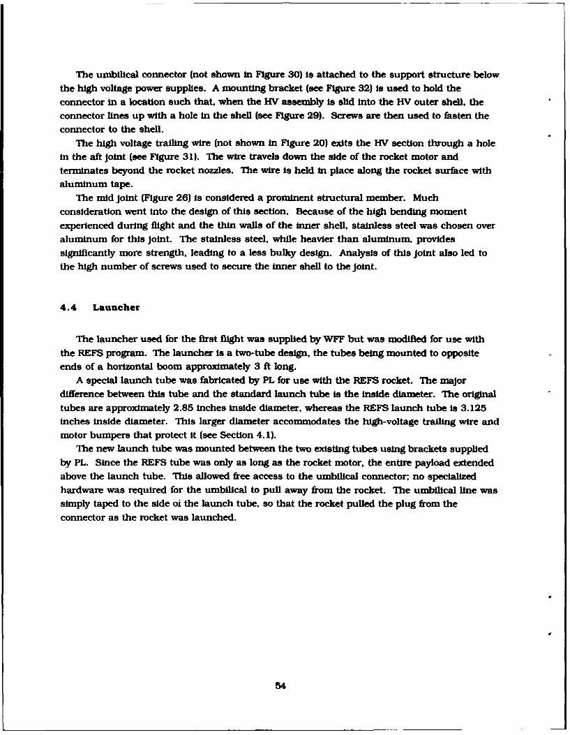
The umbilical connector (not shown in Figure 30) is attached to the support structure belowthe high voltage power supplies. A mounting bracket (see Figure 32) ts used to hold theconnector in a location such that, when the HV assembly is slid into the HV outer shell, theconnector lines up with a hole in the shell (see Figure 29). Screws are then used to fasten theconnector to the shell.

The high voltage trailing wire (not shown in Figure 20) exits the HV section through a holein the aft Joint (see Figure 3 1). The wire travels down the side of the rocket motor andterminates beyond the rocket nozzles. The wire is held in place along the rocket surface withaluminum tape.

The mid Joint (Figure 26) Is considered a prominent structural member. Much

consideration went into the design of this section. Because of the high bending momentexperienced during flight and the thin walls of the inner shell, stainless steel was chosen overaluminum for this Joint. The stainless steel, while heavier than aluminum, providessignificantly more strength, leading to a less bulky design. Analysis of this Joint also led tothe high number of screws used to secure the inner shell to the Joint.

4.4 Launcher

The launcher used for the first flight was supplied by WFF but was modified for use withthe REFS program. The launcher is a two-tube design, the tubes being mounted to oppositeends of a horizontal boom approximately 3 ft long.

A special launch tube was fabricated by PL for use with the REFS rocket. The majordifference between this tube and the standard launch tube is the inside diameter. The originaltubes are approximately 2.85 inches inside diameter, whereas the REFS launch tube is 3.125inches inside diameter. This larger diameter accommodates the high-voltage trailing wire andmotor bumpers that protect it (see Section 4.1).

The new launch tube was mounted between the two existing tubes using brackets suppliedby PL. Since the REFS tube was only as long as the rocket motor, the entire payload extended

above the launch tube. This allowed free access to the umbilical connector; no specializedhardware was required for the umbilical to pull away from the rocket. The umbilical line wassimply taped to the side oi the launch tube, so that the rocket pulled the plug from the

connector as the rocket was launched.

54

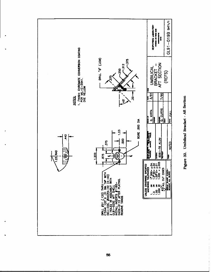
CY,

.4 IZ

-JoYLJ L

Ut.. LL -0

dliimTa

-~ Wi

0 C4

a CO)S

4 >- z-sa

xby:iO.a

55'

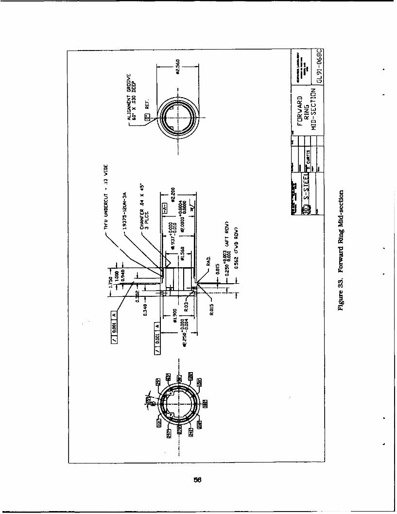
--i

Ow

z MZM I* 8-Z

CKc L. I

ZLJ-

I om

C2

3- N

Wud 00C

z in t.. u

I- .4 OL) E 0"1+ C%o ~ I - cW? CD C2

21cci

Of

C3=u

C4

f9 ~

4 56

5. PRE-FLIGHT AERODYNAMIC ANALYSIS

Before NASA allows the REFS vehicle to be launched at KSC, a complete pre-flight analysisof the aerodynamic stability and performance is necessary to determine the impact point. The

impact point at KSC is critical and must be in a lagoon that is situated between the RTLP

launch pad and a public beach. Since the FFAR had never been flown with the REFS payload,

KSC also requested that preliminary launches be performed at WFF.

The pre-flight analysis for a KSC launch was performed by Capt Carl Frushon and Capt

Robert Longstreth, both of PL/SXA. with much help from Dr. George Jumper, of the Worcester

Polytechnic Institute. The pre-flight analysis for the WFF launch was performed by Capt

Longstreth and Dr Jumper. The analysis was performed in three parts:

1. Computation of the mass properties of the 2.75-inch FFAR and REFS payload using the

Mass Properties program (MASSPROP) written by Capt C.J. Frushon of PL/SXA.

2. Determination of the aerodynamic stability derivatives using the USAF Missile

DATCOM program, 28 which was written for the Flight Dynamics Laboratory, Wright-

Patterson AFB.

3. Prediction of performance and trajectory using the NASA Goddard Space Flight Center

Missile and Satellite Simulation program2 9 (MASS). Note: To avoid confusion with

MASSPROP, we refer to MASS as SOAR (Simulation Of A Rocket). This practice will be

followed throughout this report.

Once the initial prediction of impact point was made, a complete dispersion analysis and

sensitivity study was done to study the effects of different uncontrollable variables. Theresults of this study have been included in the discussion of the performance prediction.

5.1 Computation of the Mass Properties

The mass properties of the REFS rocket were computed for two cases. The first case has afully loaded motor, and the second case has an expended motor. MASSPROP computes mass

properties by breaking the entire structure up into geometrically simple shapes, computing the

properties of each of these shapes, and then combining the properties back into a single

structure. Because of the complexity of both the REFS payload and the FFAR, the entire REFS

28 Nielsen, J.N., (1960) Missile Aerodynamics, McGraw-Hill Book Company, Inc., New York.

29 AVCO, (1974) MASS Program Users Manual, prepared for NASA Goddard Space Flight

Center, Greenbelt. MD, under Contract NAS5-23231, by AVCO Systems Division, MarylandOperations, Seabrook MD.

57

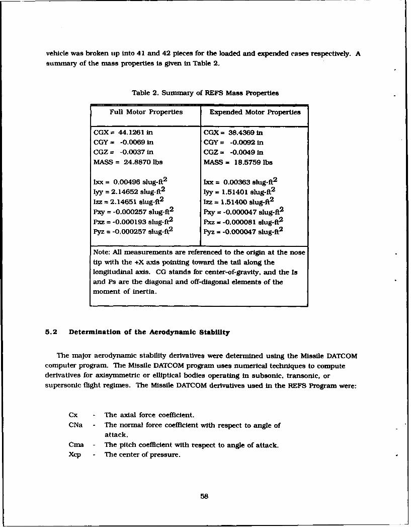
vehicle was broken up into 41 and 42 pieces for the loaded and expended cases respectively. A

summary of the mass properties is given in Table 2.

Table 2. Summary of REFS Mass Properties

Full Motor Properties Expended Motor Properties

CGX= 44.1261 in CGX= 38.4369inCGY = -0.0069 in CGY = -0.0092 in

CGZ = -0.0037 in CGZ = -0.0049 in

MASS = 24.8870 lbs MASS = 18.5759 lbs

lxx = 0.00496 slug-ft2 Ixx = 0.00363 slug-ft2

Iyy = 2.14652 slug-ft2 Iyy = 1.51401 slug-ft2Iz = 2.14651 slug-ft2 Izz = 1.51400 slug-ft2

Pxy = -0.000257 slug-ft2 Pxy = -0.000047 slug-ft2

Pxz = -0.000193 slug-ft2 Pxz = -0.000081 slug-ft2

Pyz = -0.000257 slug-ft2 Pyz = -0.000047 slug-ft 2

Note: All measurements are referenced to the origin at the nose

tip with the +X aids pointing toward the tall along thelongitudinal axis. CG stands for center-of-gravity, and the Is

and Ps are the diagonal and off-diagonal elements of the

moment of inertia.

5.2 Determination of the Aerodynamic Stability

The major aerodynamic stability derivatives were determined using the Missile DATCOM

computer program. The Missile DATCOM program uses numerical techniques to computederivatives for axisymmetric or elliptical bodies operating in subsonic, transonic, or

supersonic flight regimes. The Missile DATCOM derivatives used in the REFS Program were:

Cx - The axial force coefficient.CNa - The normal force coefficient with respect to angle of

attack.

Cma - The pitch coefficient with respect to angle of attack.

Xcp -The center of pressure.

58

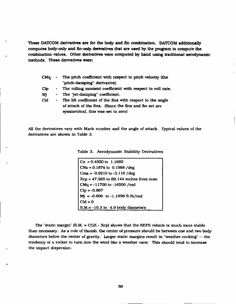
These DATCOM derivatives are for the body and fin combination. DATCOM additionallycomputes body-only and fin-only derivatives that are used by the program to compute thecombination values. Other derivatives were computed by hand using traditional aerodynamicmethods. These derivatives were:

CMq - The pitch coefficient with respect to pitch velocity (the"pitch-damping" derivative).

Clp - The rollnig moment coefficient with respect to roll rate.

MJ - The 'Jet-damping" coefficient.Cld - The lift coefficient of the fins with respect to the angle

of attack of the fins. (Since the fins and fin set aresymmetrical, this was set to zero)

AD the derivatives vary with Mach number and the angle of attack. Typical values of thederivatives are shown in Table 3.

Table 3. Aerodynamic Stability Derivatives

Cx = 0.4920 to 1.1680CNa = 0.1874 to 0.1988 /degCma = -0.9219 to -3.116 /degXcp = 47.265 to 69.144 inches from nose

CMq = -11700 to -16500 [radCIp = -0.667MJ = -0.606 to -1.1998 ft-lb/rad

Cld = 0

S.M.= -10.3 to -4.9 bodcy diameters

The "static margin" (S.M. = CGX - Xcp) shows that the REFS vehicle is much more stablethan necessary. As a rule of thumb, the center of pressure should be between one and two bodydiameters below the center of gravity. Larger static margins result in "weather-cocking" -- thetendency of a rocket to turn into the wind like a weather vane. This should tend to increasethe impact dispersion.

59

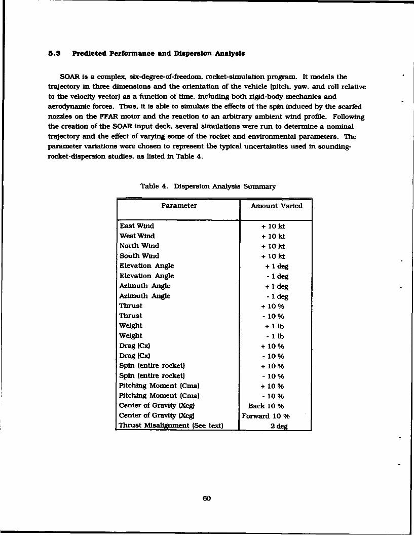
5.3 Predicted Performance and Dispersion Analysis

SOAR is a complex, six-degree-of-freedom, rocket-simulation program. It models thetrajectory in three dimensions and the orientation of the vehicle (pitch, yaw. and roll relativeto the velocity vector) as a function of time, including both rigid-body mechanics andaerodynamic forces. Thus, it is able to simulate the effects of the spin induced by the scarfednozzles on the FFAR motor and the reaction to an arbitrary ambient wind profile. Followingthe creation of the SOAR input deck, several simulations were run to determine a nominaltrajectory and the effect of varying some of the rocket and environmental parameters. Theparameter variations were chosen to represent the typical uncertainties used in sounding-rocket-dispersion studies, as listed in Table 4.

Table 4. Dispersion Analysis Summary

Parameter Amount Varied

East Wind + 10 ktWest Wind + 10 kt

North Wind + 10 ktSouth Wind + 10 kt

Elevation Angle + 1 degElevation Angle - 1 degAzimuth Angle + 1 degAzimuth Angle - 1 deg

Thrust + 10%Thrust - 10%Weight + 1 lbWeight - llbDrag (Cx) + 10%Drag (Cx) - 10%Spin (entire rocket) + 10 %Spin (entire rocket) - 10 %Pitching Moment (Cma) + 10 %Pitching Moment (Cma) - 10 %Center of Gravity (Xcg) Back 10 %Center of Gravity (Xcg) Forward 10 %Thrust Misalignment (See text) 2 deg

60

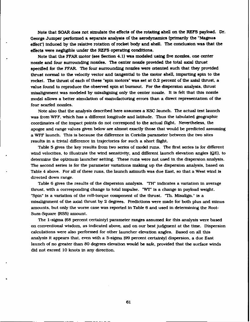
Note that SOAR does not simulate the effects of the rotating shell on the REFS payload. Dr.

George Jumper performed a separate analysis of the aerodynamics (primarily the "Magnus

effect") induced by the relative rotation of rocket body and shell. The conclusion was that the

effects were negligible under the REFS operating conditions.

Note that the FFAR motor (see Section 4.1) was modeled using five nozzles, one center

nozzle and four surrounding nozzles. The center nozzle provided the total axial thrustspecified for the FFAR. The four surrounding nozzles were oriented such that they providedthrust normal to the velocity vector and tangential to the motor shell, imparting spin to the

rocket. The thrust of each of these "spin motors" was set at 0.2 percent of the axial thrust, a

value found to reproduce the observed spin at burnout. For the dispersion analysis, thrust

misalignment was modeled by misaligning only the center nozzle. It Is felt that this nozzle

model allows a better simulation of manufacturing errors than a direct representation of the

four scarfed nozzles.Note also that the analysis described here assumes a KSC launch. The actual test launch

was from WFF, which has a different longitude and latitude. Thus the tabulated geographic

coordinates of the impact points do not correspond to the actual flight. Nevertheless, the

apogee and range values given below are almost exactly those that would be predicted assuming

a WFF launch. This Is because the difference in Coriolis parameter between the two sitesresults in a trivial difference in trajectories for such a short flight.

Table 5 gives the key results from two series of model runs. The first series is for differentwind velocities, to illustrate the wind sensitivity, and different launch elevation angles (QE). to

determine the optimum launcher setting. These runs were not used in the dispersion analysis.The second series is for the parameter variations making up the dispersion analysis, based on

Table 4 above. For all of these runs, the launch azimuth was due East, so that a West wind is

directed down range.Table 6 gives the results of the dispersion analysis. 'TH" indicates a variation in average

thrust, with a corresponding change to total impulse. 'r"W' is a change in payload weight.

"Spin" is a variation of the roll-torque component of the thrust. 'Th. Misalign." is amisalignment of the axial thrust by 2 degrees. Predictions were made for both plus and minus

amounts, but only the worse case was reported in Table 6 and used in determining the Root-

Sum-Square (RSS) amount.The 1-sigma (68 percent certainty) parameter ranges assumed for this analysis were based

on conventional wisdom, as indicated above, and on our best judgment at the time. Dispersion

calculations were also performed for other launcher elevation angles. Based on all this

analysis It appears that, even with a 3-sigma (99 percent certainty) dispersion, a due East

launch of no greater than 80 degrees elevation would be safe, provided that the surface winds

did not exceed 10 knots in any direction.

61

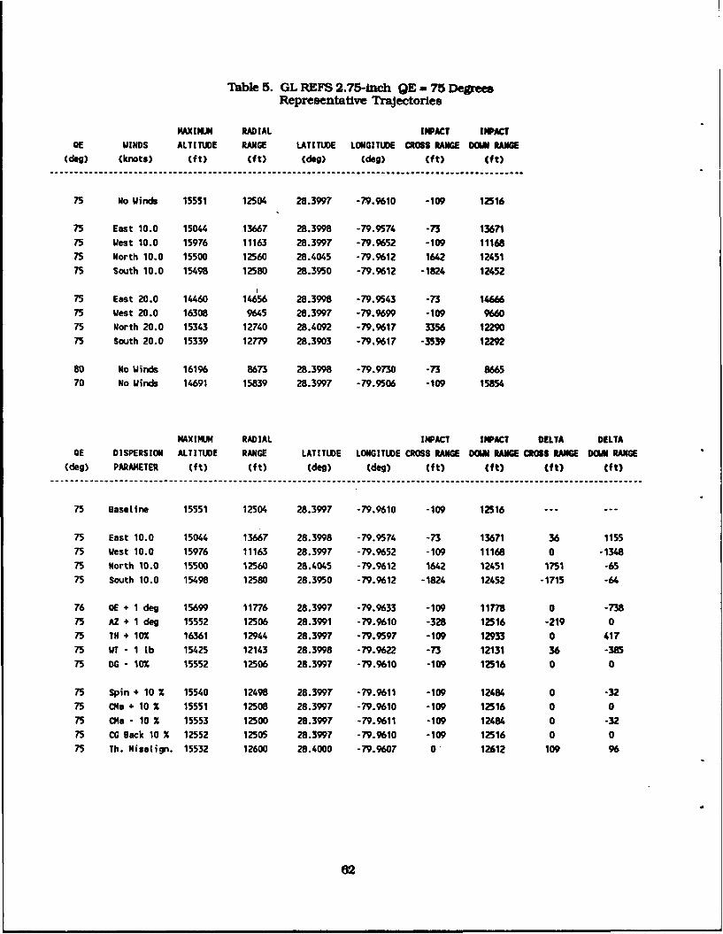
Table 5. GL REFS 2.75-inch QE = 75 DegreesRepresentative Trajectories

MAXIMUM RADIAL IMPACT IMPACTQE WINDS ALTITUDE RANGE LATITUDE LONGITUDE CROSS RANGE DOWN RANGE

(deg) (knots) (ft) (ft) (des) (des) (ft) (ft)

75 No Winds 15551 12504 28.3997 -79.9610 -109 12516

75 East 10.0 15044 13667 28.3998 -79.9574 -73 1367175 West 10.0 15976 11163 28.3997 -79.9652 -109 11168

75 North 10.0 15500 12560 28.4045 -79.9612 1642 12451

75 South 10.0 15498 12580 28.3950 -79.9612 -1824 12452

75 East 20.0 14460 14656 28.3998 -79.9543 -73 14666

75 West 20.0 16308 9645 28.3997 -79.9699 -109 966075 North 20.0 15343 12740 28.4092 -79.9617 3356 12290

75 South 20.0 15339 12779 28.3903 -79.9617 -3539 12292

80 No Winds 16196 8673 28.3998 -79.9730 -73 866570 No Winds 14691 15839 28.3997 -79.9506 -109 15854

MAXIMUM RADIAL IMPACT IMPACT DELTA DELTAOE DISPERSION ALTITUDE RANGE LATITUDE LONGITUDE CROSS RANGE DOWN RANGE CROSS RANGE DOWNI RANGE

(deg) PARAMETER (ft) (ft) (deg) (deg) (ft) (ft) (ft) (ft)

75 Baseline 15551 12504 28.3997 -79.9610 -109 12516

75 East 10.0 15044 13667 28.3998 -79.9574 -73 13671 36 115575 West 10.0 15976 11163 28.3997 -79.9652 -109 11168 0 -134875 North 10.0 15500 12560 28.4045 -79.9612 1642 12451 1751 -65

75 South 10.0 15498 12580 28.3950 -79.9612 -1824 12452 -1715 -64

76 OE + 1 deg 15699 11776 28.3997 -79.9633 -109 11778 0 -73875 AZ + 1 deg 15552 12506 28.3991 -79.9610 -328 12516 -219 0

75 TN + 10% 16361 12944 28.3997 -79.9597 -109 12933 0 41775 WT - 1 Lb 15425 12143 28.3998 -79.9622 -73 12131 36 -385

75 DG - 10" 15552 12506 28.3997 -79.9610 -109 12516 0 0

75 Spin + 10 % 15540 12498 28.3997 -79.9611 -109 12484 0 -32

75 CMa + 10 % 15551 12508 28.3997 -79.9610 -109 12516 0 075 Cma - 10 % 15553 12500 28.3997 -79.9611 -109 12484 0 -32

75 CG Back 10 % 12552 12505 28.3997 -79.9610 -109 12516 0 0

75 Th. Misatign. 15532 12600 28.4000 -79.9607 0 12612 109 96

62

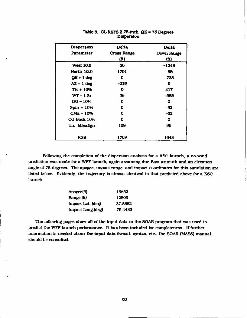
Table 6. GL REFS 2.75-inch QE -75 DegreesDispersion

Dispersion Delta DeltaParameter Cross Range Down Range

Mft} (ft)West 10.0 36 -1348

North 10.0 1751 -65QE + deg 0 -738AZ+ I deg -219 0TH + 10% 0 417WT- 1 b 36 -385DG - 10% 0 0

Spin + 10% 0 -32CMa- 10% 0 -32

CG Back 10% 0 0Th. Misakgn 109 96

RSS 1769 1643

Following the completion of the dispersion analysis for a KSC launch, a no-windprediction was made for a WFF launch, again assuming due East azimuth and an elevationangle of 75 degrees. The apogee, impact range, and impact coordinates for this simulation arelisted below. Evidently, the trajectory is almost identical to that predicted above for a KSClaunch.

Apogee(ft) 15552Range (ft) 12505Impact lat. (deg) 37.8382Impact Long. (deg) -75.4433

The following pages show all of the input data to the SOAR program that was used topredict the WFF launch performance. It has been included for completeness. If furtherinformation is needed about the input data format, syntax, etc., the SOAR (MASS) manualshould be consulted.

63

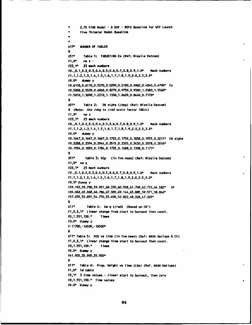
* 2.75 FFAR Model - 6 DOF - REFS Baseline for UFF Launch* Five Thruster Model Baseline

X17* MUKBER OF TABLESSX51* Table 1: THRUSTING Cx (Ref: Missile Datcom)

F1.0' no -F23.1* 23 mach numbersFO.,0.1*0.2,0.3,0.4*0.5.0.6.0.7,0.8,0.9. 1.0' Mach nu.ers

F0.0' &mAy yF0.6110,0.61 10,0.5570,O.5290,0.5100,0.4960*0.4840,0.4790' CxF0.5000,0.5520,0.6960,0.8270,0.9750,0.9380, 1.2080,1.5560*Fl .5010.1.3690,1.2210,1.1330.1.0620.0.8460.0.7170*

X51* Table 2: CN alpha (/deg) (Ref: Missile Datcom)S (Note: Use /deg to /rad scale factor 180/c)P1,0' no zF23.1* 23 mach numbersFO..0.1.0.2,0.3,0.4,0.5,0.6,O.7.0.8,O.9,1.0' Machi numbrersF1.1*l.2,1.3,1.4,1 .5,1.6,1.7.1.8.1.9.2.0.2.5.3.0*F0.0* dmvW yF0.1647.0.1647,0.1667,0.1703,0.1759,0.1838,0.1955,0.2211* CN alphaFO.228,0.2394,0.2944,0.2515.0.2355,0.2430.0.2078,0.2016'FO.1934.0.1850.0.1784,0. 1725.0.1688.0.1398.0.1171*SX51* Table 3: XCp (in frm nose) (Ref: Missile Datcom)F1,0' no zP23,1' 23 mach numbersFO.,0.1.0.2,0.3.0.4,0.5.0.6.0.7,0.8,0.9, 1.0* Mach numb~ersP1.1,1.2,1.3,1.4,1.5,1.6,1.7,1 .8.1.9.2.0.2.5.3.0*F0.0* Dummy yP59.192,59.700,59.931,60.330,60.908,61.709.62.733.64.582* CPF65.062,65.068,66.786,67.383.69.144.63.88559.571.58.846*P57.035,55.891.54.770.53.690,52.822,48.328.47.265*

SX11* Table 4: Cm q (/rad) (Based on CM')

F1.0,3,1* Linear change from start to burnout then const.F0.1.551.100.* TimesF0.0* Dummy yF-11700, .16500.. 16500*SXli' Table 5: XCG vs time (in ft. nose) (Ref- NASA Wallops CF V)P1.0,3,1* Linear change from start to burnout then const.F0.1.551.100.- TimesP0.0' Dumort yF41.905.35.905.35.905*

X11* Table 6: Prop. Weight vs Time (Lbs) (Ref. NASA Wallops)F1.0' Id tableF3,1* 3 time values - linear start to burnout, then zeroP0.1.551.100.' Time values

F0.0* Duuwp' y

64

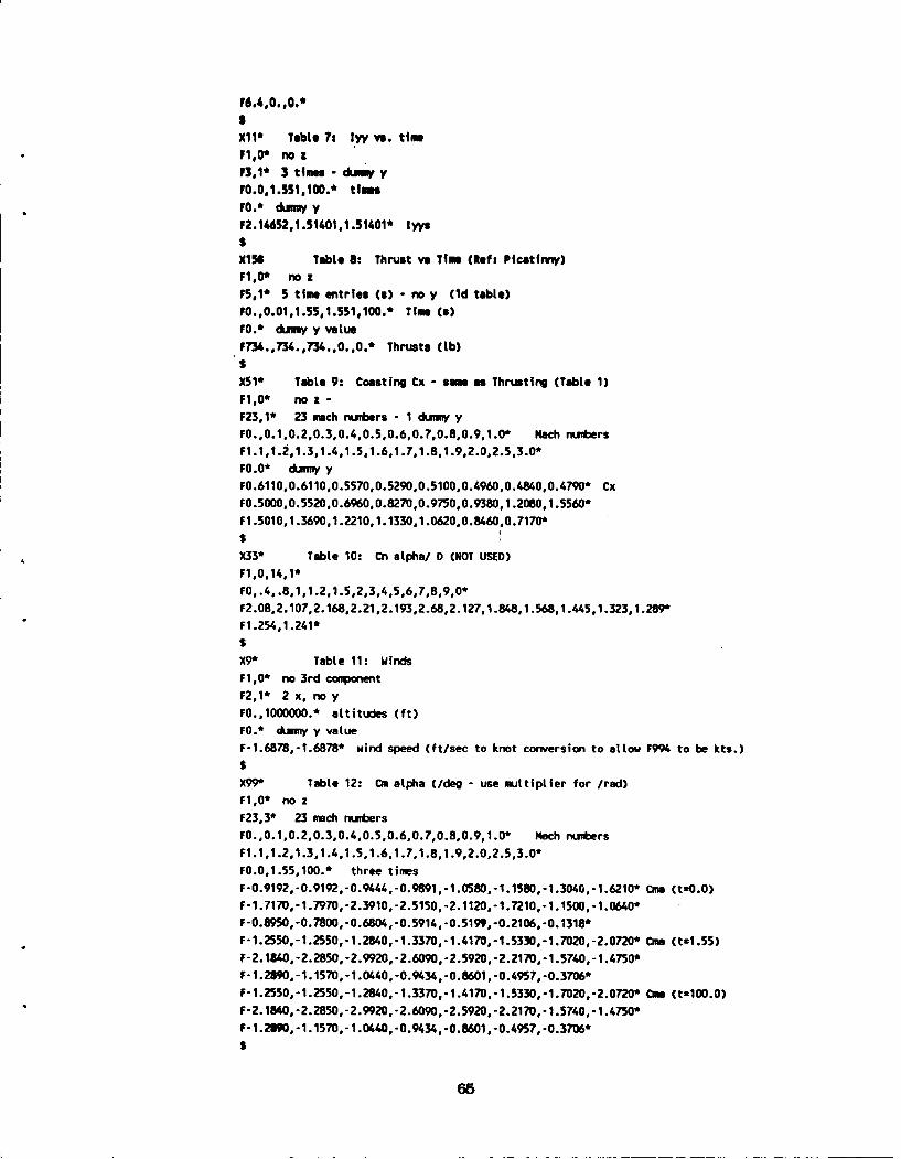
P6.4,0., .0.S

xII* Table 7s Iyy vs. timeP1,0' no aP3,1' 3 times - &Miv yPO.0,1.551,100.* time"

P0.' d.uuy y

SX154 Table 8: Thrust vs TIm CRef: Picatinny)P1.0' no zP5,1' 5 time entries (a) - no y Cid table)PO.,0.01,1.55,1.551,100.' Time (s)P0.' dauny y value

P734.,734.,734.,0.,0.' Thrusts (Lb)

X51' Table 9: Coasting Cx - same as Thrusting (Table 1)

P1,0' no z

F23,1' 23 mach ruriers - Ilduu yyFO.,0.1,0.2,0.3,0.4,0.5,0.6,0.7,0.8,0.9,1.0' Kach nu. rsP1.1.1.2,1.3,1.4,1.5.1.6,1.7,1.8,1.9,2.0,2.5,3.0'FO.0' &urmy yFO.6110,0.6110,0.5570,0.5290,0.5100,0.496O,0.4840,0.4790* CxFO.5000.0.5520,a.6960.0.8270,0.9750,0.9380, 1.2080,1.5560'F1.5010,1.3690.1..2210,1.1330,1 .0620.0.8460,0.7170'S

4X33* Table 10: Cn alpha/ 0 (NOT USED)F ,O, 14, 1'FO,.4..5,1,1.2,1.5 .2,3,*4, 5,6,7,8.9,0'F2.08, 2. 107, 2. 168, 2.21,2. 193 .2.68, 2. 127, 1.848, 1.568, 1.445,1.323,1. 289'Fl .254,1.241'

X9' Table 11: WindsP1,0' no 3rd component

F2.1' 2 x,no y

F0.' &~muy y value

F-1.6878,-1.6878' wind speed (ft/sec: to knot conversion to allow F994 to be kts.)S

X99' Table 12: COn alpha (/deg - use multtiplier for /red)F1,0' no z

F23,3' 23 mach numibersFO.,0.1,0.2,0.3,0.4,0.5,0.6,0.7,0.8,0.9,1.0' Hach nunbersP1.1,1.2,1.3,1.4,1.5,1.6,1.7,1.8,1.9,2.0,2.5,3.0'

F0.0,1.55,100.' three timesF-0.9192,-0.9192,-0.94"4,-0.9891 ,-1.058D,-1.1580,-1 .3040,-1.6210* One (t.0.0)P-i .7170,-i .7970, -2.3910, -2.5150, -2. 1120,-i .7210.-i. 1500,-i .0640'F-0.8950,-0.780, -0.6804,-0.5914, -0.5199,-0.2106,-0. 1318'P-1.2550,-1.2550,-1.2840,-1.3370,-1.4170,-1.5330,-1.7020,-2.0720* Cne (tul .55)F-2.1840,-2.2850,-2.9920,-2.6090,-2.5920,-2.21-0,-1.5740.-1.4750*P- .2890,-1. 1570,-i 0440, -0.91.34, -0.8601. -0.4957, -0.3706'F-1.2550,-1.2550,-1.2840,-1.3370,-1.4170,-1.5330,-1.7020,-2.0720* Ce. (t=100.0)P-2. 1840,-?. 2850,- 2.9920, -2.6090, -2.5920, -2. 2170),-1.5740, -1.4750'P-1 .290,-i1.1570,-i1.0I.40,-0.9434, -0.8601 ,-0.4957,-0.3706'S

65

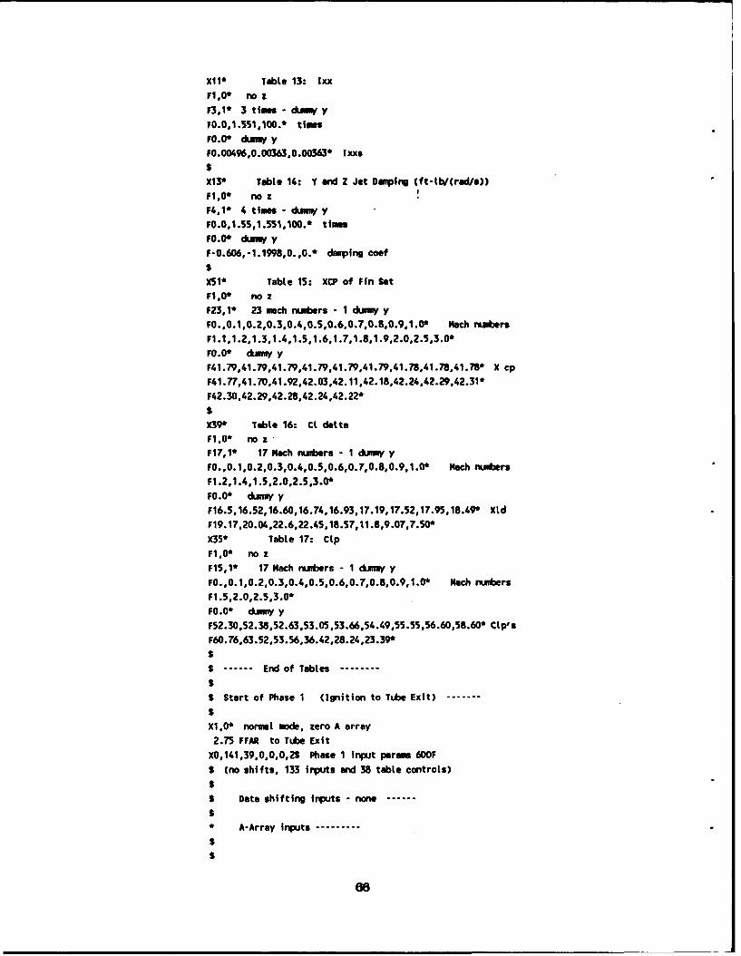
Xli' Tabte 13: lxx

FI,0' no z

F3.1' 3 times - du y

FO.0,1.551.100.* timesFO.0' dijmu y

F0.OO'.96,0.00363,0.00363* lxxs

X13' Tabte 14: Y and Z Jet Damping (ft-lb/Crad/e))FI,0' no zF4,1* 4 times - uwujyyFO.0,1.55,1.551,¶00.' timesFO.0' dumm yF-0.606,-1.1998,0.,0.* damping coef

SX(51* Tabte 15: XCP of Fin Set

F1.0' no zF23.1* 23 machnu~ibers - I dtVyyFO. .0.1,0.2,0.3,0.4,0.5.0.6,0.7.0.8.0.9,.1.0 Mach ntikers

F1.1,1.2.1.3,1.4,1.5,1.6,1.7,1.8.1.9,2.0,2.5.3.0*

FO.0' dunmy yF41.79,41.79,41.79,41.79,41.79,41.79,41.78,41 .78.41.78* X cp

F41.77,41. 70,41 .92,42.03 ,42. 11,42. 18.42. 24 .42.29,42.31-

F42.30,42.29,42. 28.42.24,42.22'SX(39' Tabte 16: Cl deltaF1,0' no zF17.1* 17 Mach ruibers;- 1 dLWyyFO..0.1,0.2,0.3,0.4.0.5,0.6,0.7,0.8,0.9,1.0' Mach numb~ersFl.2.1 .4.1.5.2.0.2.5,3.0'FO.0' djmW yF16.5. 16.52,16.60,16.74,16.93,17.19,17.52,17.95,18.49' KldF19.17,20.0f.,22.6,22.45,18.57,11 .8,9.07.7.50'X35* Table 17: Ctp

F1,0' no zF15,1* 17 Mach ru.brs - I1dumy y

FO.,0.1,0.2,0.3,0.4,0.5,0.6,0.7,0.8,0.9,1.0' Mach rnwbers

Fl .5,2.0.2.5.3.0'

FO.0' &rnuy y

F52.30,52.38.52.63,53.05,53.66,54.49,55.55.56.60,58.60* CLp's

F60.76,63.52,53.56,36.42,28.24,23.39*

S........End of Tables---------

S Start of Phase 1 (ignition to TIte Exit)----

Xl.0' normat mode. zero A array2.75 FFAR to UbAe Exit

XO,141,39.0.0.0,2$ Phase 1 input perams 60OFS (no shifts, 133 inputs and 38 table controls)

S Data shifting irpijts - none .---

S

' A-Array inputs........-

66

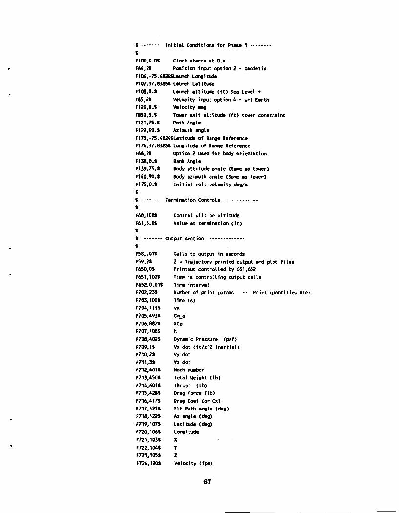
S ---- initial Conditions for Phase 1 ----

F100,O0. Clock starts at 0.3.F64,2s Position input option 2 -GeodeticF106,-75.4834$aunchd LongitudeF107,37.aM$5 Launch LatitudeF1O8,0.S Laun~ch attitude (ft) Sea Level +F65,f.S Velocity input option 4 - wrt EarthF120,03S Velocity MagF850,53S Tower exit altitude (ft) tower constraintF121,753. Path Angle

F122,903S Azimuth angleF 173.-iS .4824SLati tude of Range ReferenceF174,37.83a55 Longitude of Range ReferenceF66,2$ option 2 used for body orientationF138,0.S lank AngleF139,75.$ Body attitude angle (Same as tower)

F140903S Body azimu~th angle (Same as tower)

F175.O.S Initial roil velocity deg/s

SS -------- Termination Controls------------SF60,108S Control will be altitudeF61,5.OS Value at termination (ft)SS-------- Output section-------------SF58'.O1S Calls to output in secondsF59,2S 2 = Trajectory printed output and plot filesF650,0$ Printout controlled by 651,652F651,100S Time is controlling output ca'llsF652,.OO1S Time interval

F702,23S Number of print params -- Print quantities are:F703,100S Time (s)

1704,1115 Vx

F705,493S CMa8

F706,887S XCpF707,108% h

F708,402S Dynamic Pressure (psf)F709,1S Vx dot (ft/s^2 inertial)F710,25 Vy dotF711,3* Vz dot1F712,401S Mach numb~erF713,450S Total Weight (ib)F714,601% Thrust (Ib)F715,4.28* Drag Force (Ib)F716,4175 Drag Coef (or Cx)F717,i21S fit Path angle (deg)

F718,122S Az angle (deg)

F719,1075 Latitude (deg)

F720,106S LongitudeF721,103S xF722,104$ YF723,105S ZF724,1205 Velocity (fps)

67

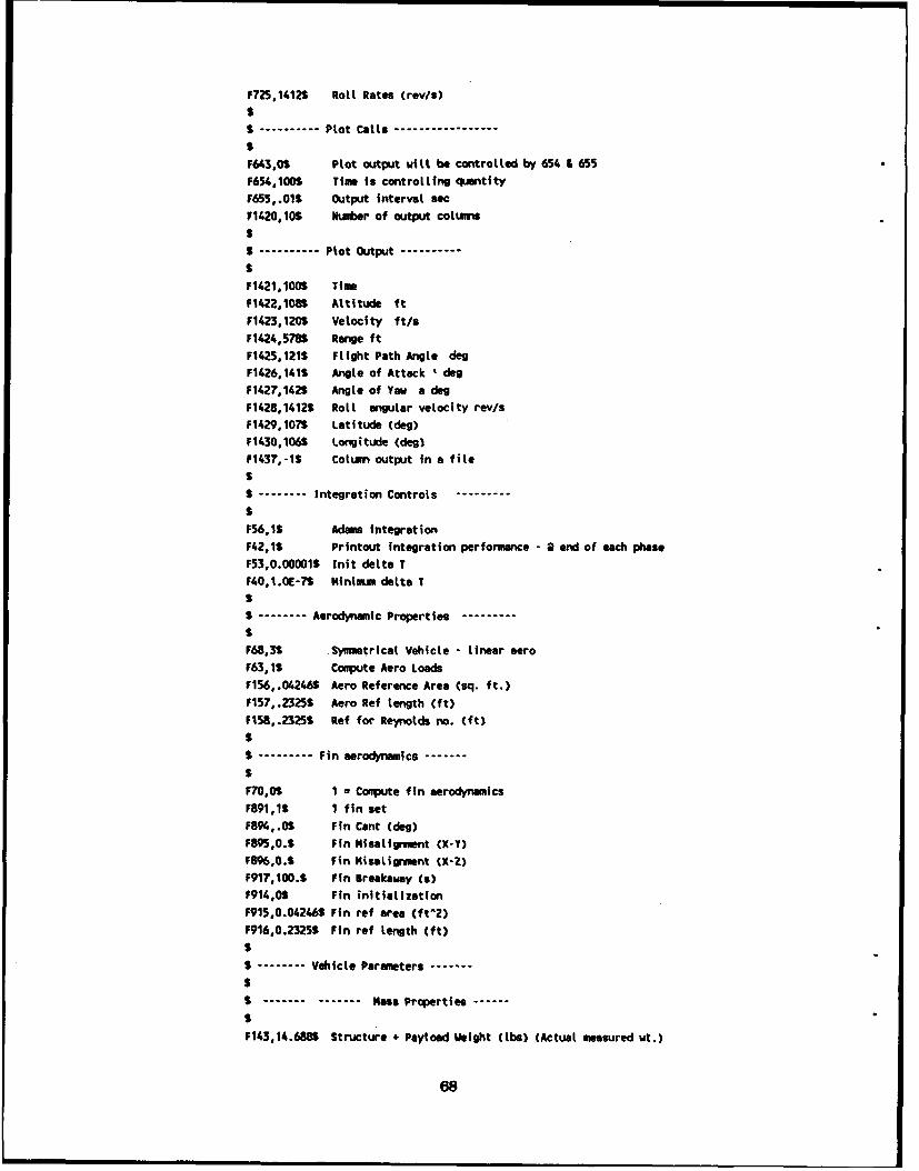
F725.1412S Roll Rates (rev/a)

SS ----------Plot Cotlls----------------SF643.OS Plot output will be controLted by 654 &655

F654,1C001 Time is controlling quantityF655,.01S Output interval, aftF1420. 10S Nwiber of output coluwaSS ---------- Plot OuItput........--SF14.21,100% TimeF1422,108S Alttitude ftF1423,120S Velocity ft/s

F1424,578S Range ftF1425* 121S Flight Path Angle degF1426*1411 Angle of Attack I degF1427,142S Angle of Yaw a degF1428.1412% Roll angular velocity rev/sF1429,107S Latitude (deg)F1430,106$ Longitude (deg)F1437,-IS Column output in a fileSS -------- Integration Controls -----SF56.1$ Adams IntegrationF42,1S Printout integration performance 2 end of each phaseF53,O.OOOO1$ Init delta TF40* ¶.OE-7S Minimum de~ta TSS -------- Aerodynamic Properties---------SF68,3$ .Symmetricat Vehicle - linear aeroF63,1% Compute Aero LoadsF156,.04246$ Aero Reference Area (sq. ft.)F¶57#.2325S Aero Ref length (ft)

Fl5Se.2325S Ref for Reynolds no. (ft)SS1--------- F in aerodynamnics;----SP70,0S 1 aCompute f in aerodynami cs

F891,11 1 fin setF894,.O$ Fin Cant (deg)F895,031 Fin Misalignment (X-Y)F896,0.3 fin Misatiwwrint (X-Z)F917, 100.1 Fin Breakaway (s)F914,OS Fin initializationF915,0.042465 Fin ref area (ft^2)F916,0.2325$ Fin ref length (ft)SS -------- Vehicle Parameters ----S-------- -------- Mass Properties ---

F143,14.6805 Structur* + Payload Weight (tbs) (Actual measured wt.)

68

$

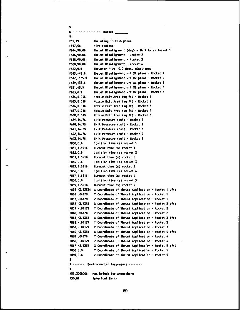
-------- -------- Rocket$

F55,1$ Thrusting in this phase

F597,5S Five rocketsF614,90.0S Thrust Misaligrvnhnt (deg) with X Axis- Rocket 1

F616,90.0$ Thrust Misaligruent - Rocket 2

F618,90.0S Thrust MisaLignment - Rocket 3

F620,90.0S Thrust Misalignment - Rocket 4

F622,0.3 Thruster Five 0.0 degs. misaligned

F615,45.3 Thrust Misalignment wrt XZ plane - Rocket 1

F617,-135.3 Thrust MisaLigrnent wrt XZ plane - Rocket 2

F619.135.3 Thrust Misalignment wrt XZ plane - Rocket 3

F621,45.3 Thrust Misalignment wrt XZ plane - Rocket 4

F603,03. Thrust Misalignment wrt XZ plane - Rocket 5F634,0.01$ Nozzle Exit Area (sq ft) - Rocket 1

F63S,0.01S Nozzle Exit Area (sq ft) - Rocket 2

F636,0.01$ Nozzle Exit Area (sq ft) - Rocket 3

F637,0.01$ Nozzle Exit Area (sq ft) - Rocket 4

F638,0.01S Nozzle Exit Area (sq ft) - Rocket 5

F639,14.7$ Exit Pressure (psi) - Rocket 1

F610,14.73 Exit Pressure (psi) - Rocket 2

F641,14.7% Exit Pressure (psi) - Rocket 3

F642,14.7S Exit Pressure (psi) - Rocket 4

F643,14.7% Exit Pressure (psi) - Rocket 5

F830,0.3 Ignition time (s) rocket 1

F831,1.551$ Burnout time (s) rocket 1

F832,0.$ ignition time (s) rocket 2

F833,1.5515 Burnout time (s) rocket 2F834,0.3 Ignition time (M) rocket 3

F835,1.551S Burnout time (s) rocket 3

F836,0.$ Ignition time (s) rocket 4

F837,1.551$ Burnout time (s) rocket 4

F838,0.3 Ignition time (s) rocket 5

F839,1.551$ Burnout time (s) rocket 5

F855,-3.3333$ X Coordinate of Thrust Application - Rocket 1 (ft)

F856,.0417S Y Coordinate of Thrust Application - Rocket 1

F857,.04175 Z Coordinate of Thrust Application - Rocket 1

F858,-3.3335 X Coordinate of Thrust Application - Rocket 2 (ft)

F859,-.0417$ Y Coordinate of Thrust Application - Rocket 2

I60,.0417S Z Coordinate of Thrust Application - Rocket 2

F&M1,-3.333$ X Coordinate of Thrust Application - Rocket 3 (ft)

F"82,o.0417$ Y Coordinate of Thrust Application - Rocket 3

F863,-.04173 Z Coordinate of Thrust Application - Rocket 3F864,-3.333$ X Coordinate of Thrust Application - Rocket 4 (ft)

F865,.0417% Y Coordinate of Thrust Application - Rocket 4

F866,-.04175 Z Coordinate of Thrust Application - Rocket 4

F867,-3.3335 X Coordinate of Thrust Application - Rocket 5 (ft)

F868,0.$ Y Coordinate of Thrust Application - Rocket 5

F869,0.3 Z Coordinate of Thrust Application - Rocket S3

S ------- Environmental Parameters --------S

F53,300000S Max heigth for Atmosphere

F50,03 Spherical Earth

69

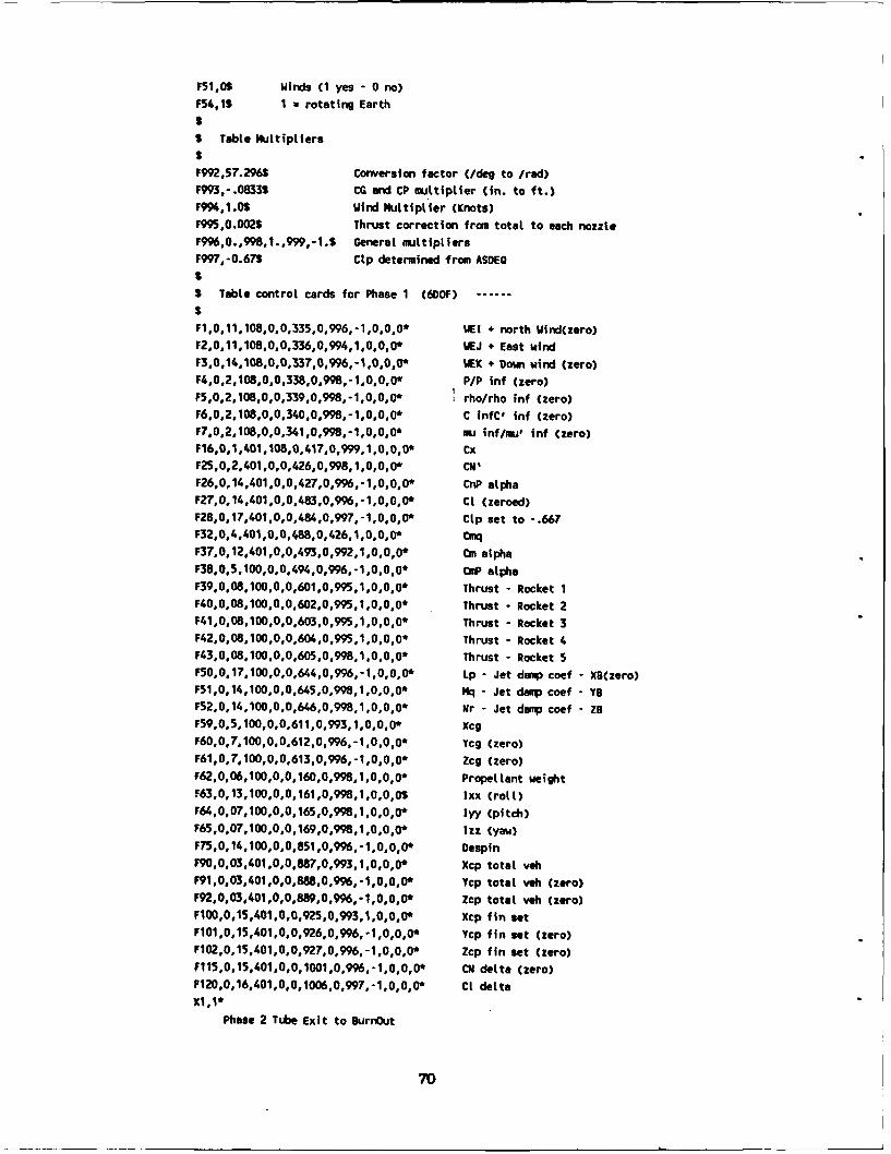
F51,05 Winds (1 yes - 0 no)

F54,15 1 a rotating Earth

S

S Table Multipliers

SF992,57.296$ Conversion factor (/deg to /red)F9M,3-.0833S CG and CP multiplier (in. to ft.)F994,1.0S Wind Multiplier (Knots)F995,0.002S Thrust correction fram total to each nozzle

F996,0.,998,1.,999,-1.S General multipliersF997,-0.67S Ctp determined from ASDEQ

$S Table control cards for Phase 1 (6DOF)

$F1,0,11,108,0,0,335,0,996,-1,0.0,0" WEI + north Wind(zero)F2,0,11,108,0,0,336,0,994,1,0,0.0- WEJ + East wind

F3,0,14,108,0,0,337,0,996,-1,0,0,0 WEK + Dowm wind (zero)F4,0,2,108o0,0,338,0,998,-1,0,0,0, P/P inf (zero)F5,0,2,108,0,0,339,0,998,-1,0,0,0* rho/rho inf (zero)F6,0,2,108.0,0,340,0,998,-1,0,0,0* C |nfC' inf (zero)F7,0,2,108,0,0,341,0,998,-1,0,0,0 mu inf/mu, inf (zero)F16,0,1,401,108,0,417,0,999,1,0,0,0* Cx

F25,0,2,401,0,0,426,0,998,1,0,0,0* CNI

F26,0,14,401,0,0,427,0,996,-1,0,0,0* CnP alphaF27,0,14,401,0,0,483,0,996,-1,0,0,0* CI (zeroed)

F28,0,17,401.0,0,484,0,997,-1,0,0,0* Ctp set to -. 667F32,0,4,401,0,0,488,0,426,1,0,0,0* CRK

F37,0,12,401,0,0,493,0,992,1,0,0,0" On alphaF38,0,5,100,0,0,494,0,996,-1,0,0,0" CmP alpha

F39,0,08,100.0,0,601,0,995,1.0,0,0" Thrust Rocket 1F40,0,08,100,0,0,602,0,995,1,0,0,0* Thrust Rocket 2F41,0,08,100,0,0,603.0,995,1,0,0,0* Thrust Rocket 3F42,0,08,100,0,0,604,0,995,1,0,0,0, Thrust Rocket 4F43,0,08,100,0,0,605,0,998.1,0.0,0* Thrust - Rocket 5

F50,0,17,100,0,0,644,0,996,-1,0,0,0' Lp - Jet daop coef - XB(zero)F51,0,14,100,0,0,645,0,998,1,0,0,0, Mq - Jet da'p coef - YB

F52,0,14,100,0,0,646,0,998,1,0,0,0* Nr - Jet damp coef - Z9

F59,0,5,100,0,0,611,0,993,1,0,0,0" XcgF60,0,7,100,0.0.612.0.996,-1.0,0,o0 Ycg (zero)

F61,0,7,100,0,0,613,0,996,-1,0,0,0. Zcg (zero)F62,0,06,100,0,0,160,0,998,1,0,0,0" Propellant weightF63,0,13,100,0,0,161,0,998,1,0,0,0$ Ixx (rotl)F64,0,07,100,0,0,165,0,998,1,0,0,0* lyy (pitch)F65,0,07,100,0,0,169,0,998,1,0,0,0" Izz (yaw)

F75,0,14,100,0,0,851,0,996,-1,0,0,0" DespinF90,0,03,401,0,0,887,0,993,1,0,0,0* Xcp total vehF91,0,03,401,0,0,888,0,996,-1,0.0,0" Ycp total vah (zero)

F92,0,03,401,0,0,889,0,996,-1,0,0,0* Zcp total veh (zero)FOO,0,15,401,0,0,925,0,993,1,0,0,0" Xcp fin setF101,0,15,401,0,0,926,0,996,-1,0,0,0* Ycp fin set (zero)F102,0,15,401,0,0,927,0,996,-1,0,0,0* Zcp fin set (zero)

F115,0,15,401,0,0,1001,0,996,-1,0,0,0* CM delta (zero)F120,0,16,401,0,0,1006,0,997,-1,0,0,0" Ct delta

Xl,'"

Phase 2 Tube Exit to BurnOut

70

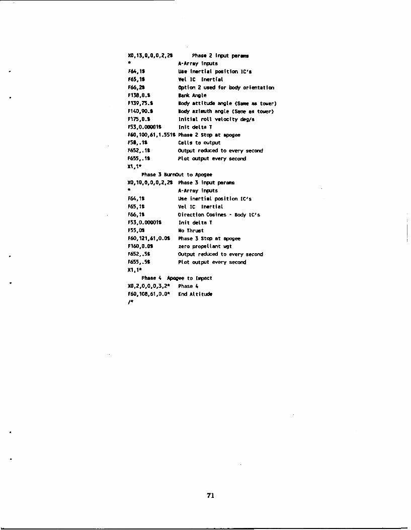
X0.13,0,0,0,2,2S Phase 2 input paramsA-Array Inputs

F64,1$ Use Inertial position IC's

F65,1$ Val IC Inertial

F66,2S option 2 used for body orientationF138,0.3 Bank Angle

F139,75.3 Body attitude angle (Sane as tower)F140,90.$ Body azimuth angle (Same as tower)

F175,0.$ Initial roll velocity deg/s

F53,0.000011 Init delta TF60,100,61,1.551$ Phase 2 Stop at apogee

F58,.1S Calls to outputF652,.15 Output reduced to every second

F655,.1$ Plot output every second

X1,1"

Phase 3 BurnOut to Apogee

XO,10,0,0,0,2,2$ Phase 3 input perems

A-Array inputsF64,1$ Use inertial position IC's

F65,15 Vel IC Inertial

F66,1S Direction Cosines - Body IC'sF53,0.000015 [nit delta T

F55,0$ No Thrust

F60,121,61,0.0$ Phase 3 Stop at apogee

F160,0.0$ zero propellant wgtF652, .55 Output reduced to every second

F655,.5S Plot output every second

X1,1*Phase 4 Apogee to Impact

XO,2,0,0,0,3,2* Phase 4

F60,108,61,0.0* End Altitude

/*

71

6. FIELD-MEASUREMENT THEORY AND CALIBRATION

6.1 Theory of Measurement

The theory of measuring ambient electrostatic field from an aircraft with multiple fieldmills is well developed and has been discussed recently by Laroche, 2 7 Bailey and Anderson,2 6

and Kositsky et al.2 4 Here we outline the basic ideas in the context of our rocket design.Imagine a right-handed, Cartesian coordinate system aligned so that the z.axis lies along

the longitudinal (symmetry) axis of the rocket, pointing in the direction of flight (see Figure 4).The x- and y-axes are then similar and transverse to the rocket axis. Consider first ahomogeneous (over dimensions large compared to those of the rocket), steady (over timescomparable to one shell-rotation period) electric field component Ez directed in the positive z

direction. When the rocket is placed in this ambient field, it distorts the field locally in amanner described by Laplace's equation (with boundary conditions specifying a uniform fieldat infinity and zero potential over the surface of the rocket). Since Laplace's equation islinear, its solution for the surface field contribution F, at any set of points on the rocket body(the locations of the field mills) due to component E. can be expressed as follows:

F, = ajzEz

F"2 = a2z

(1)

Fs = aszEz

Next, suppose that a homogeneous, electrostatic field component E, Is directed in the

positive x direction. Again, Laplace's equation gives the field contribuilon at the same set ofpoints on the rocket body, the only difference in the boundary conditions being the directionof the uniform field at Infinity. This yields another set of coefficients ai,. Similarly, asolution can be obtained for an electric field component Ey in the positive y direction. Finally,

Laplace's equation can be solved for zero ambient field and potential at infinity but a uniformpotential V on the rocket, giving the coefficients aiv. (It should be noted that these potential

coefficients have different units from the field coefficients.) By the superposition principle,these four solutions can be added to obtain the total field Fi at each mill due to an arbitrary

ambient vector field E (or to an arbitrary orientation of the rocket) and an arbitrary net

charge (Q = CV, where C is the capacitance) on the rocket:

72

F, = a1 xEx + ajyEy + a1 zEz + a1vV

F2 = a2xEx + a2yEy + a2zEz + a2,V(2)

F8 = asxEx + a8yý + a8zEz + asvV

Obviously, Eq. (2) can be expressed in matrix notation. Extending the definition of the

vector E to include the potential V as its fourth component, we have

F = AE (3)

where A is an 8x4 matrix of constants (for a particular rocket geometry). Assuming the

symmetry of the rocket described in Section 4.2, we can write this equation as follows:

0 aty atz atv

F tr •0 -aty at, atv

Ft d 0 amy amz amv

mr 0 -my a i m y VF E0m 0 -a abz abv E

Fbr = a(4)

Fbi 0)Fa 0 a a

re|my mz my

Fmb -a 0 am amy

The first subscripts t, m, and b refer to the top, middle, and bottom longitudinal

positions along the payload, while the second subscripts r.l.t. and b refer to the right, left, top,

and bottom azimuthal positions around its circumference, looking up the tail of the rocket

(along the positive z axis). By symmetry, the right and left azimuthal positions see no Ex and

73

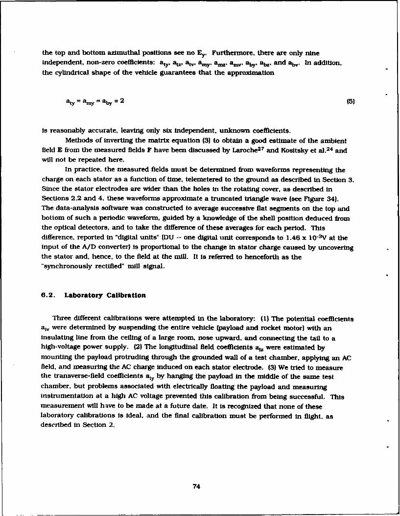
the top and bottom azimuthal positions see no Ey. Furthermore, there are only nineindependent, non-zero coefficients: aty, atz, at, amy, amz, am, aby, ab,, and abv. In addition,the cylindrical shape of the vehicle guarantees that the approximation

Sty= amy = aby =2 (5)

is reasonably accurate, leaving only six independent, unknown coefficients.Methods of inverting the matrix equation (3) to obtain a good estimate of the ambient

field E from the measured fields F have been discussed by Laroche27 and Kositsky et al. 24 and

will not be repeated here.In practice, the measured fields must be determined from waveforms representing the

charge on each stator as a function of time, telemetered to the ground as described in Section 3.Since the stator electrodes are wider than the holes in the rotating cover, as described inSections 2.2 and 4, these waveforms approximate a truncated triangle wave (see Figure 34).The data-analysis software was constructed to average successive fiat segments on the top andbottom of such a periodic waveform, guided by a knowledge of the shell position deduced fromthe optical detectors, and to take the difference of these averages for each period. Thisdifference, reported in "digital units" (DU -- one digital unit corresponds to 1.46 x 10-3V at theinput of the A/D converter) is proportional to the change in stator charge caused by uncoveringthe stator and, hence, to the field at the mill. It is referred to henceforth as the"synchronously rectified" mill signal.

6.2. Laboratory Calibration

Three different calibrations were attempted in the laboratory: (1) The potential coefficientsaiv were determined by suspending the entire vehicle (payload and rocket motor) with anInsulating line from the ceiling of a large room, nose upward, and connecting the tail to ahigh-voltage power supply. (2) The longitudinal field coefficients a1z were estimated bymounting the payload protruding through the grounded wall of a test chamber, applying an ACfield. and measuring the AC charge induced on each stator electrode. (3) We tried to measurethe transverse-field coefficients a1y by hanging the payload In the middle of the same testchamber, but problems associated with electrically floating the payload and measuringInstrumentation at a high AC voltage prevented this calibration from being successful. Thismeasurement will have to be made at a future date. It is recognized that none of theselaboratory calibrations is ideal, and the final calibration must be performed in flight, asdescribed in Section 2.

74

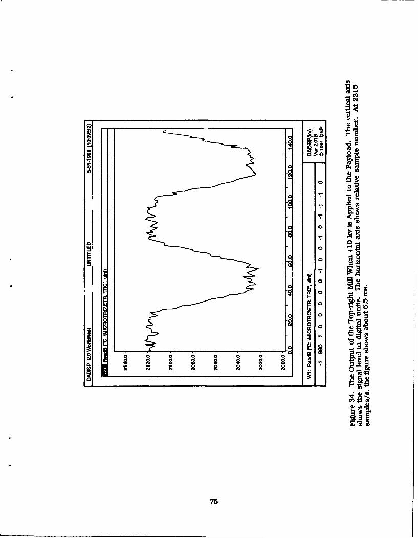
InIom

ol - ------- r

9 9

lIt

75

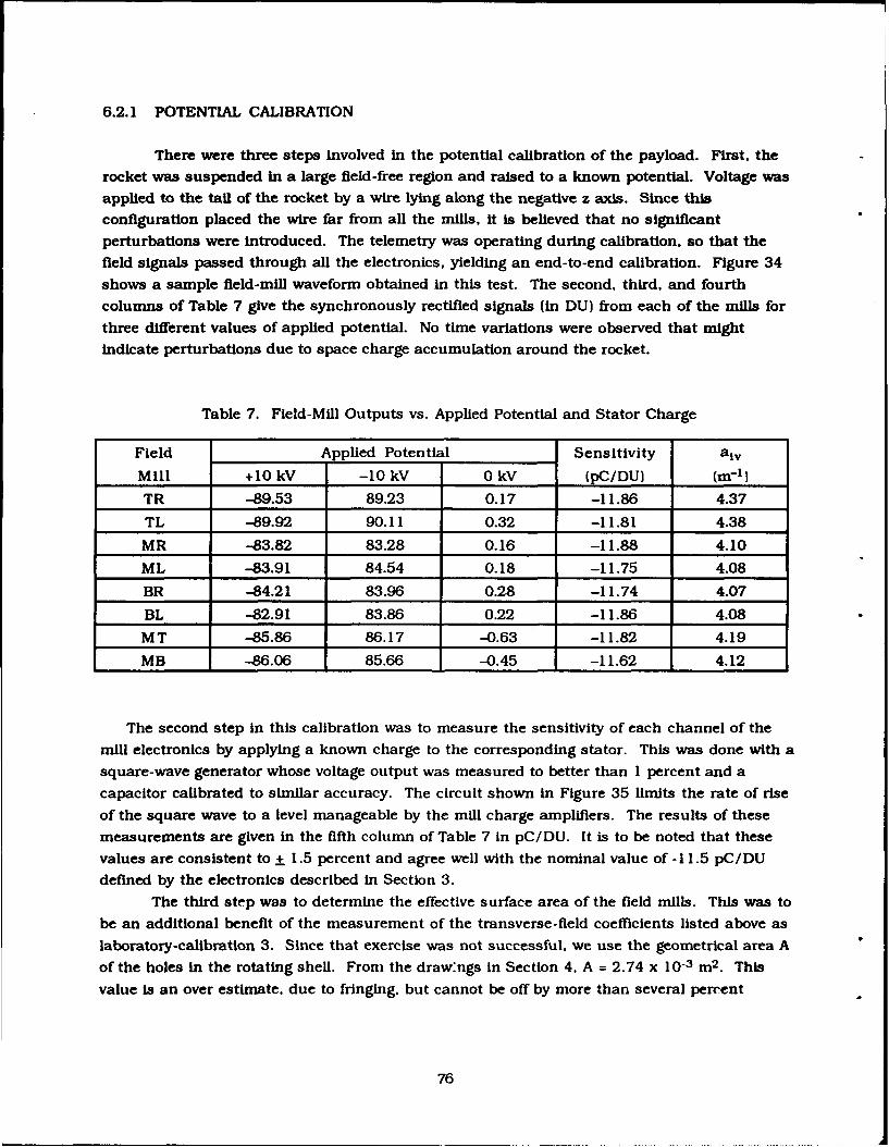
6.2.1 POTENTIAL CALIBRATION

There were three steps involved in the potential calibration of the payload. First, the

rocket was suspended in a large field-free region and raised to a known potential. Voltage was

applied to the tall of the rocket by a wire lying along the negative z axis. Since this

configuration placed the wire far from all the mills, it is believed that no significant

perturbations were introduced. The telemetry was operating during calibration, so that the

field signals passed through all the electronics, yielding an end-to-end calibration. Figure 34

shows a sample field-mill waveform obtained in this test. The second, third, and fourth

columns of Table 7 give the synchronously rectified signals (in DU) from each of the mills for

three different values of applied potential. No time variations were observed that might

indicate perturbations due to space charge accumulation around the rocket.

Table 7. Field-Mill Outputs vs. Applied Potential and Stator Charge

Field Applied Potential Sensitivity alv

Mill +10 kV -10 kV 0 kV (pC/DU) (r-l)

TR -89.53 89.23 0.17 -11.86 4.37

TL -89.92 90.11 0.32 -11.81 4.38

MR -83.82 83.28 0.16 -11.88 4.10

ML -83.91 84.54 0.18 -11.75 4.08

BR -84.21 83.96 0.28 -11.74 4.07

BL -82.91 83.86 0.22 -11.86 4.08

MT -85.86 86.17 -0.63 -11.82 4.19

MB -86.06 85.66 -0.45 -11.62 4.12

The second step in this calibration was to measure the sensitivity of each channel of the

mill electronics by applying a known charge to the corresponding stator. This was done with a

square-wave generator whose voltage output was measured to better than I percent and a

capacitor calibrated to similar accuracy. The circuit shown in Figure 35 limits the rate of rise

of the square wave to a level manageable by the mill charge amplifiers. The results of these

measurements are given in the fifth column of Table 7 in pC/DU. It is to be noted that these

values are consistent to + 1.5 percent and agree well with the nominal value of -11.5 pC/DU

defined by the electronics described in Section 3.

The third step was to determine the effective surface area of the field mills. This was to

be an additional benefit of the measurement of the transverse-field coefficients listed above as

laboratory-calibration 3. Since that exercise was not successful, we use the geometrical area A

of the holes in the rotating shell. From the draw'ngs In Section 4. A = 2.74 x 10-3 m 2 . This

value is an over estimate, due to fringing, but cannot be off by more than several percent

76

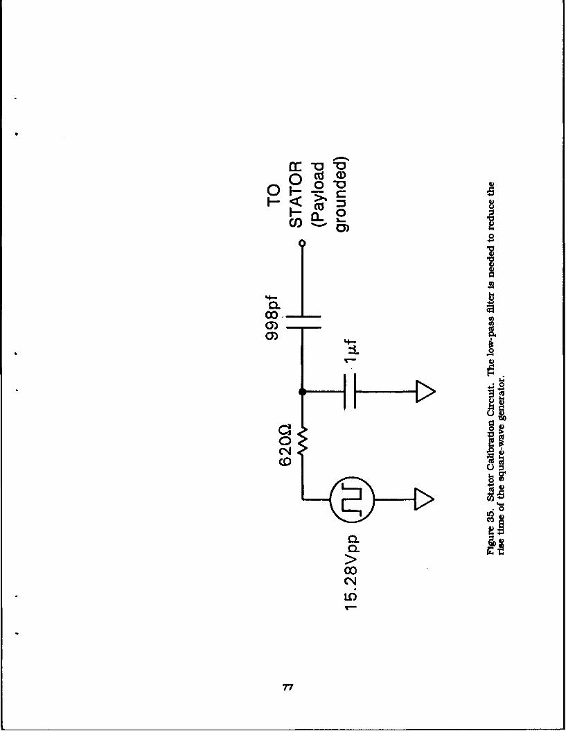
a: -0

0a.CO

0)CYJ

(0

"CEO

0. C00

Co4

77

because the rotor-to-stator spacing is only a small fraction of the other dimensions of thehole. Since the surface field is related to the stator charge by

F = Q/e0 A (6)

where Eo = 8.85 x 10-12 is the dielectric permittivity of air, the voltage coefficients of thevarious mills can be tabulated in the last column of Table 7 in units of m-1 . The values fordifferent mills at the same longitudinal position are quite consistent, as they should be, exceptperhaps for mill MT. which seems about 2 percent high. Note that the absolute values of thesecoefficients are not Important because the voltage on the rocket is not a very useful number.Their relative values are unaffected by our over estimate of A. and they can be checked inflight by virtue of the on-board charging system.

6.2.2 LONGITUDINAL FIELD CALIBRATION

The only large electric-field-calibration chamber readily available to us was located at theNaval Research Laboratory (NRL) in Washington, DC. The chamber is an 11 ft cube of whichone wall is grounded, an arbitrary potential can be applied to the opposite wall, and the otherfour sides consist of overlapping guard rings. These rings are connected to successive steps of aresistor ladder between the grounded and active walls to reduce fringing effects by forcing auniform field along the sides. The entire assembly is shielded from external fields by agrounded Faraday cage. The use of this chamber has been described by Gathman 30 He kindlymade it available to us.

Because the NRL chamber was too small to encompass the whole REFS vehicle withoutintroducing significant errors due to image effects in the walls, it was decided to approximatefree-field conditions by mounting the payload so that it protruded half a rocket length throughthe grounded wall. It is well known that an uncharged conductor immersed in a uniform fieldperpendicular to a plane of symmetry can be correctly represented by replacing one half-spacewith a grounded plane located in the symmetry plane. Although the rocket is not perfectlysymmetrical about any plane perpendicular to its longitudinal axis, the difference betweennose cone and tail fins can be neglected to a good approximation, since they are far apartcompared to the difference in their dimensions. Thus, there will be a zero-potential surfacethat is nearly planar and cuts the vehicle near the center of its longitudinal axis. The overalllength of the REFS vehicle is about 82 in. from nose tip to fin tip (with the fins deployed inflight configuration), so measurements were made with the payloud protruding 39-1/2, 41, and42-1/2 in. from the chamber wall.

Space charge will accumulate in such a calibration chamber when a DC field is applied -- aresult of the "electrode effect". In the worst case, this can lead to a decrease of about a factor of

30 Gathman, S.G. (1968) Guarded double field meter, Rev. ScL Instr. 39:43-47.

78

2 in the field Intensity at the center of the chamber relative to that at the walls. In order to

eliminate any errors due to the electrode effect, we performed our calibration in an AC field.This was accomplished by stopping the rotating shell, so as to center its holes precisely over

the stator plates, and measuring the AC charge induced on the stators by the applied field. To

verify that subtraction of the charge induced with the stators fully covered by the rotor, as

performed in normal operation of the payload, was unnecessary, measurements were made inthe covered position also. In every case, the charge induced on a covered stator was more thantwo orders of magnitude less than that on the same stator uncovered.

The data were taken with 1045 VRMS at 419 Hz across the chamber, producing a peak

ambient field of about 441 V/m. To record the alternating charge induced on the stators bythis alternating field, the normal electronics were removed from the payload. Each stator inturn was connected by shielded cable to a charge amplifier followed by a bandpass filter and

peak detector (see Figure 36). All eight shielded cables were led down the interior of the

payload and out the rear, behind the grounded wall of the chamber. While one stator was beingmeasured, all the others were grounded.

The measuring circuit delivered a voltage V, proportional to the peak charge on each of

the stators. The peak charge induced on a circular plate of area Aflush = 3.90 x 10-3 M2 , flush-

mounted in the grounded wall was also measured, with the payload removed. Any scale factors

that might have been introduced by peculiarities of the measuring circuit or its response to theroughly sinusoidal, chamber-voltage waveform were canceled by recording ratios of stator toflush-mounted charge density, again assuming the stator effective area A given above:

at. = F'I/Ez = (Vi/A)/(Vflush/Aflush) (7)

The resulting values of the longitudinal field coefficients are given in Table 8 for the three

different mounting positions of the payload. Again, the values for different mills at the samelongitudinal position are quite consistent. The different values for longitudinal offsets of +1.8

percent (relative to the overall rocket length) around the geometric center give some idea of theuncertainty of these coefficients due to the measurement technique. Compared with these

differences, which range from +5 percent at the top mills to +12 percent at the bottom, theabsolute under-estimate of a12 due to our incorrect value of A is probably insignificant.

Obviously, a better calibration is needed here.

79

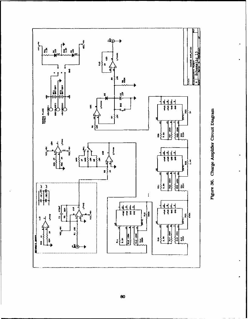
* K K - -) -- C nn az�j �- z�

09-.-'

a

iK Ua � a

- "a

.9

II IIa �iFIJ 4

a aa a

a 0 - 5

I ..

Ii.9-h

K UC a - a sot4 ft *4 .9-i

a p a Lab' C)

IW* .9.N a -

U

0

*9 .9 40

a..9 .9 .90an

Oa.9 aa.

.. a� U

80

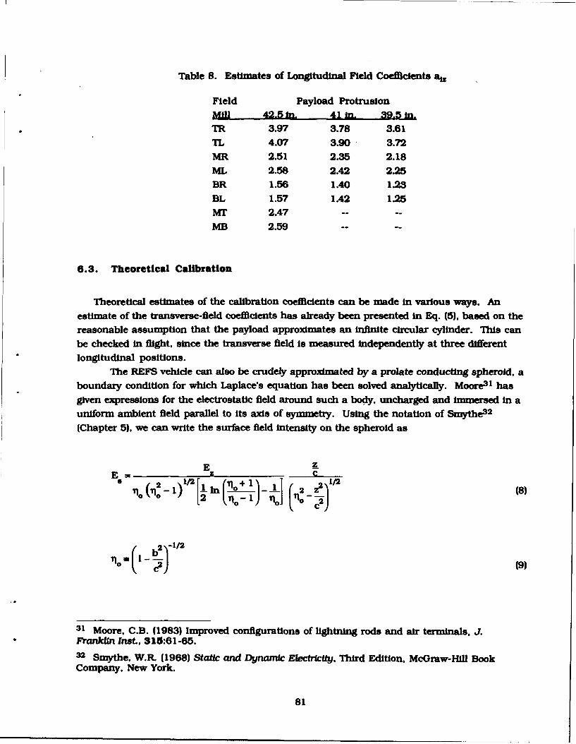
Table 8. Estimates of Longitudinal Field Coefficients a.

Field Payload Protrusionll 42.5 In. 41 in. 39.5NI.

TR 3.97 3.78 3.61TL 4.07 3.90 3.72MR 2.51 2.35 2.18ML 2.58 2.42 2.25BR 1.56 1.40 1.23BL 1.57 1.42 1.25Mr 2.47 -- --

MB 2.59 ....

6.3. Theoretical Calibration

Theoretical estimates of the calibration coefficients can be made in various ways. An

estimate of the transverse-field coefficients has already been presented in Eq. (5), based on the

reasonable assumption that the payload approximates an Infinite circular cylinder. This can

be checked in flight, since the transverse field is measured independently at three differentlongitudinal positions.

The REFS vehicle can also be crudely approximated by a prolate conducting spheroid, aboundary condition for which Laplace's equation has been solved analytically. Moore3 l hasgiven expressions for the electrostatic field around such a body, uncharged and immersed in auniform ambient field parallel to its axis of symmetry. Using the notation of Smythe32

(Chapter 5), we can write the surface field intensity on the spheroid as

E zE -=- 2)1/2 I +2

31 Moore, C.B. (1983) Improved configurations of lightning rods and air terminals, J.F'rankWn Inst., 315:61-65.

32 Smythe. W.R. (1968) Static and Dynamic EkecICtrItJ, Third Edition, McGraw-Hill BookCompany, New York.

81

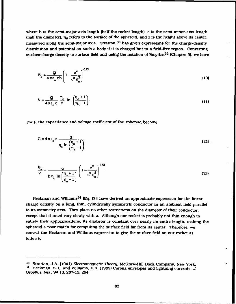
where b is the semi-major-axis length (half the rocket length). c is the semi-minor-axis length(half the diameter), 1o refers to the surface of the spheroid, and z is the height above its center,

measured along the semi-major axis. Stratton,3 3 has given expressions for the charge-density

distribution and potential on such a body if it is charged but in a field-free region. Converting

surface-charge density to surface field and using the notation of Smythe,3 2 (Chapter 5), we have

9 ( 2 -1/2E Q I- Z

c 4 ocb c2 2 (10)

4 ne c 2 (11)

Thus, the capacitance and voltage coefficient of the spheroid become

C=4ne c 2o 10 In 10 (12)

E = 2 Z_22-1/2.

V bul ln j (1 c2 19'/ (13)

Heckman and Williams34 [Eq. (2)] have derived an approximate expression for the linear

charge density on a long, thin, cylindrically symmetric conductor in an ambient field parallel

to its symmetry axis. They place no other restrictions on the diameter of their conductor,

except that it must vary slowly with z. Although our rocket is probably not thin enough to

satisfy their approximations, its diameter is constant over nearly its entire length, making the

spheroid a poor match for computing the surface field far from its center. Therefore, we

convert the Heckman and Williams expression to give the surface field on our rocket as

follows:

33 Stratton. J.A. (1941) Electromagnetic Theory, McGraw-Hill Book Company, New York.34 Heckman, S.J., and Williams, E.R. (1989) Corona envelopes and lightning currents, J.Geophys. Res., 94:13, 287-13. 294.

82

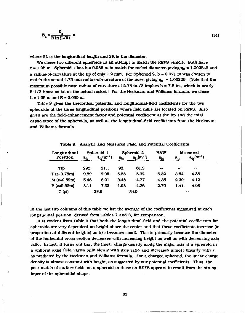
% Eln z (14)ES" Rln (L/R)

where 2L is the longitudinal length and 2R is the diameter.We chose two different spheroids in an attempt to match the REFS vehicle. Both have

c = 1.05 m. Spheroid 1 has b = 0.035 m, to match the rocket diameter, giving io = 1.000549 and

a radius-of-curvature at the tip of only 1.2 mm. For Spheroid 2. b = 0.071 m was chosen tomatch the actual 4.75 mm radius-of-curvature of the nose, giving Io = 1.00226. (Note that the

maximum possible nose radius-of-curvature of 2.75 in./2 implies b = 7.5 in., which is nearly5-1/2 times as fat as the actual rocket.) For the Heckman and Williams formula, we chose

L = 1.05 m and R = 0.035 m.Table 9 gives the theoretical potential and longitudinal-field coefficients for the two

spheroids at the three longitudinal positions where field mills are located on REFS. Alsogiven are the field-enhancement factor and potential coefficient at the tip and the total

capacitance of the spheroids, as well as the longitudinal-field coefficients from the Hecknmanand Williams formula.

Table 9. Analytic and Measured Field and Potential Coefficients

Longitudinal Spheroid I Spheroid 2 H&W MeasuredPosition a1z aiz(m"1) aiz aiz(m"1) aiz az atz(m-1 )

TIp 293. 211. 92. 61.9 .. .. ..

T (z=0.75m) 9.89 9.96 6.28 5.92 6.32 3.84 4.38M (z=0.52m) 5.48 8.01 3.48 4.77 4.35 2.39 4.12B (z=0.32m) 3.11 7.33 1.98 4.36 2.70 1.41 4.08

C (pO) 28.6 34.5 --

In the last two columns of this table we list the average of the coefficients measured at each

longitudinal position, derived from Tables 7 and 8, for comparison.It is evident from Table 9 that both the longitudinal-field and the potential coefficients for

spheroids are very dependent on height above the center and that these coefficients Increase (inproportion at different heights) as b/c becomes small. This is primarily because the diameter

of the horizontal cross section decreases with increasing height as well as with decreasing axisratio. In fact, it turns out that the linear charge density along the major axis of a spheroid ina uniform axial field varies only slowly with axis ratio and Increases almost linearly with z.

as predicted by the Heckman and Williams formula. For a charged spheroid, the linear chargedensity Is almost constant with height, as suggested by our potential coefficients. Thus, thepoor match of surface fields on a spheroid to those on REFS appears to result from the strong

taper of the spheroidal shape.

83

6.4 Summary of Matrix Coefficients

In summary, our current best estimates of the matrix coefficients in Eq. 4 are:

0.00 2.0 3.8 4.380.00 -2.0 3.8 4.38

0.00 2.0 2.4 4.12A= 0.00 -2.0 2.4 4.12 (15)

0.00 2.0 1.4 4.080.00 -2.0 1.4 4.08

2.0 0.00 2.4 4.12-2.0 0.00 2.4 4.12

Refinement of these numbers will have to await actual flight data in high fields.

7. TEST FLIGHT

7.1 Post-Flight Aerodynamic Analysis

The REFS rocket was launched from Wallops Flight Facility, Virginia, on 5 November,1990, at 2036 UT. The launcher azimuth and elevation angles were 130 and 75 degrees,respectively. The flight lasted 61 seconds. WFF used multiple radars to track the REFSpayload. Because of the small size and high acceleration of the vehicle, however, the firstradar was not able to lock on until 8 seconds Into the flight. This part of the report will

discuss how the predicted performance compared to the actual performance, as determinedfrom the radar data.

After the launch, a new model run was made based on the actual flight conditions, (thatis, observed profile of wind speed and direction, launcher elevation and azimuth, launcherlatitude and longitude, and air temperature). The actual and predicted apogee and range are

compared below:

Actual Predicted Percent Error

Apogee (ft) 12936 14981 15.8Range (ft) 13833 14286 3.3

84

Recall that the no-wind prediction in Section 5.3 was for an apogee of 15,552 ft and range of12,505 ft -- higher and shorter than either the actual or the present prediction. At launchtime, the wind was blowing at 16 ft/s from 162 degrees at the surface and was increasing and

turning toward the South with height. Because of the large static margin of the REFS rocket,this head wind caused the rocket to "weather cock" into the wind. thereby reducing its effectiveelevation angle and causing it to fly lower and longer than predicted. Evidently. the computermodel accounted fairly well for this wind effect.

The next four figures compare the actual and predicted (including wind effects) trajectoriesfor this flight. The observed (actual) curves in each figure can be recognized by the fact that thefirst approximately 8 seconds of the trajectory are missing from the radar data. Figure 37shows the predicted and actual altitudes vs elapsed time. Throughout the flight the rocket waslower than predicted, and the flight duration was shorter than predicted. Figures 38 and 39show that, at any given time, the predicted range and velocity rere very close to their actualvalues. Thus, the thrust/drag functions used in our computer model agree well with the actualrocket. Figure 40 presents the comparison in the form of altitude versus range.

7.2 Payload Mechanical Performance

The accelerometer was intended to be used for a number of measurements, includingacceleration and deceleration profiles and rocket-motor ignition and burn-out times. Usingthese data, it would be possible to calculate parameters such as maximum velocity and dragcoefficient. Some of these measurements could not be performed, however, due to thesaturation and calibration problems described in Section 3.3 above. Nevertheless, the

accelerometer did provide an accurate indication of time of launch, which will be criticalduring the program's operational phase, and the duration of motor bum (1.5 seconds).

The magnetic field sensor operated as planned. As mentioned before, the rocket motorutilizes scarfed nozzles to apply spin during the bum phase of the flight. The data obtainedshowed no unexpected results. A maximum spin rate of 17 RPS occurred at motor bum out (seeFigure 41). Rapid rotational deceleration was noted after motor burnout until the vehiclereached a steady spin rate of about I RPS throughout the remainder of the flight (see Figure42).

85

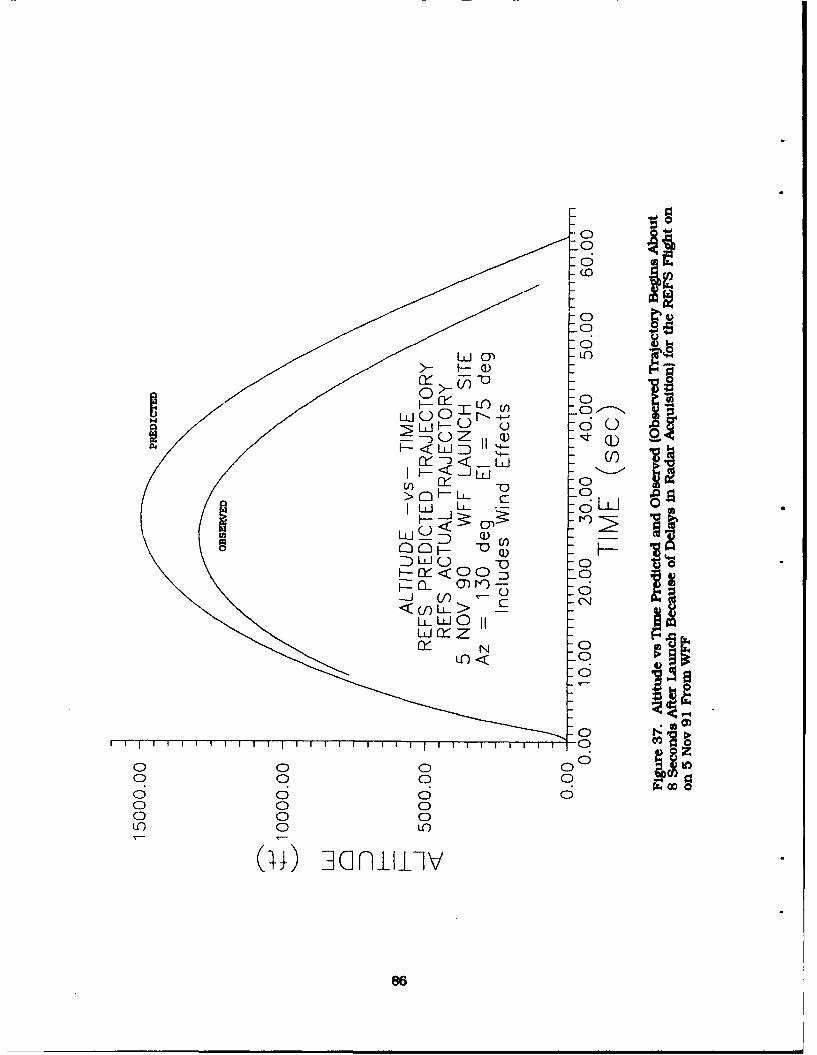
Cii_(.0

o 0 0

o 0 00 0 0

Ini 0 = I !2n.,

86 F C . _6 C

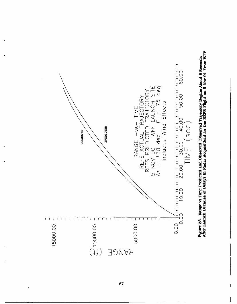
*000 OD

I-LC 0) 1 clFn< -az 10 0

00[-- :3 Ln V

n _ L C !)

0 ý- ) 0

WCo)> C 0

LLK 11 1-0

0

0D 0 (D 0C0 0 00

0 0 00f 0 10

(u1) IIONVJl

87

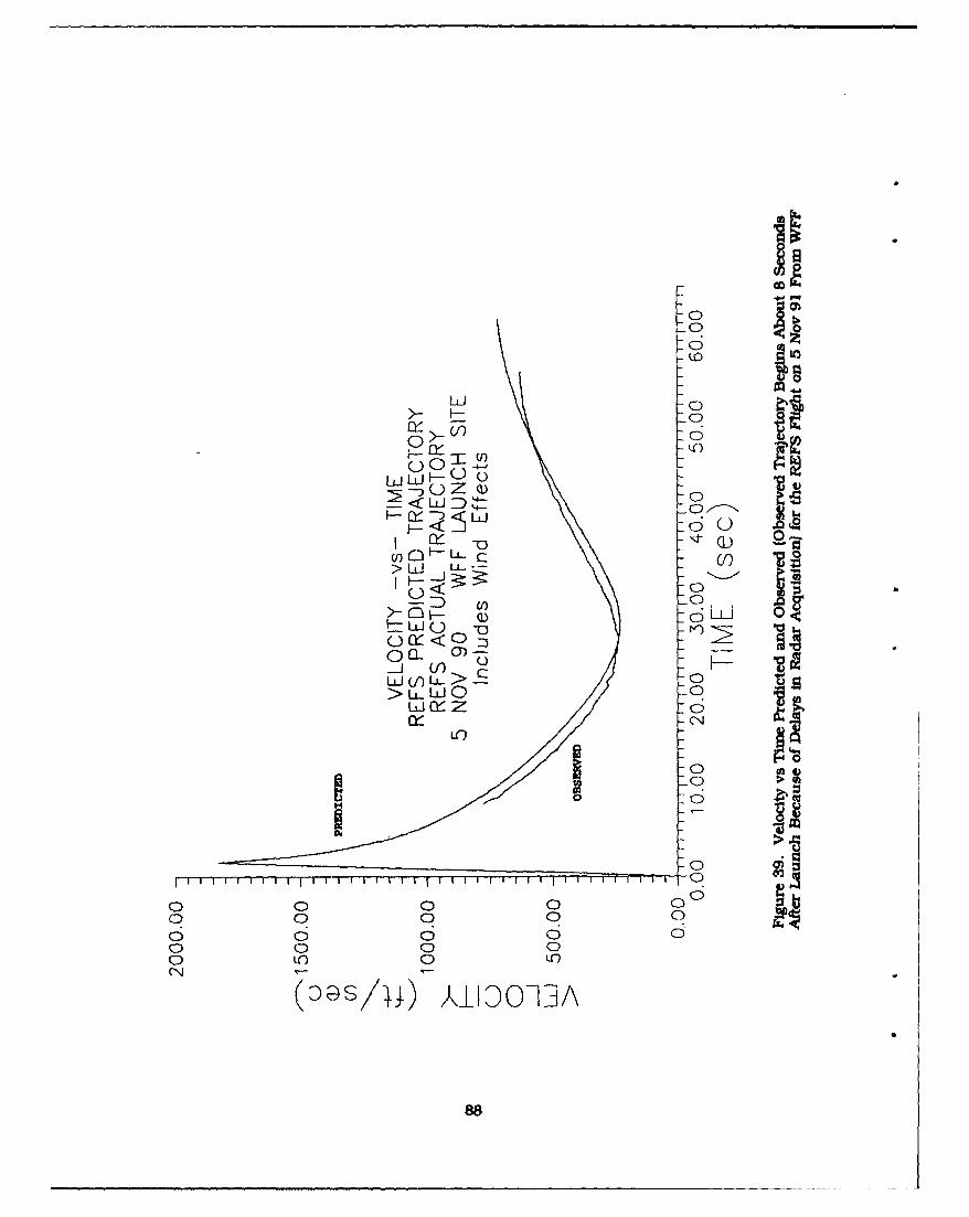
I-

00

D 4-0

1L 00

0 LL0

-0

0) 0 0 0 Il

0 ~~V Cf 0I

NnC

880

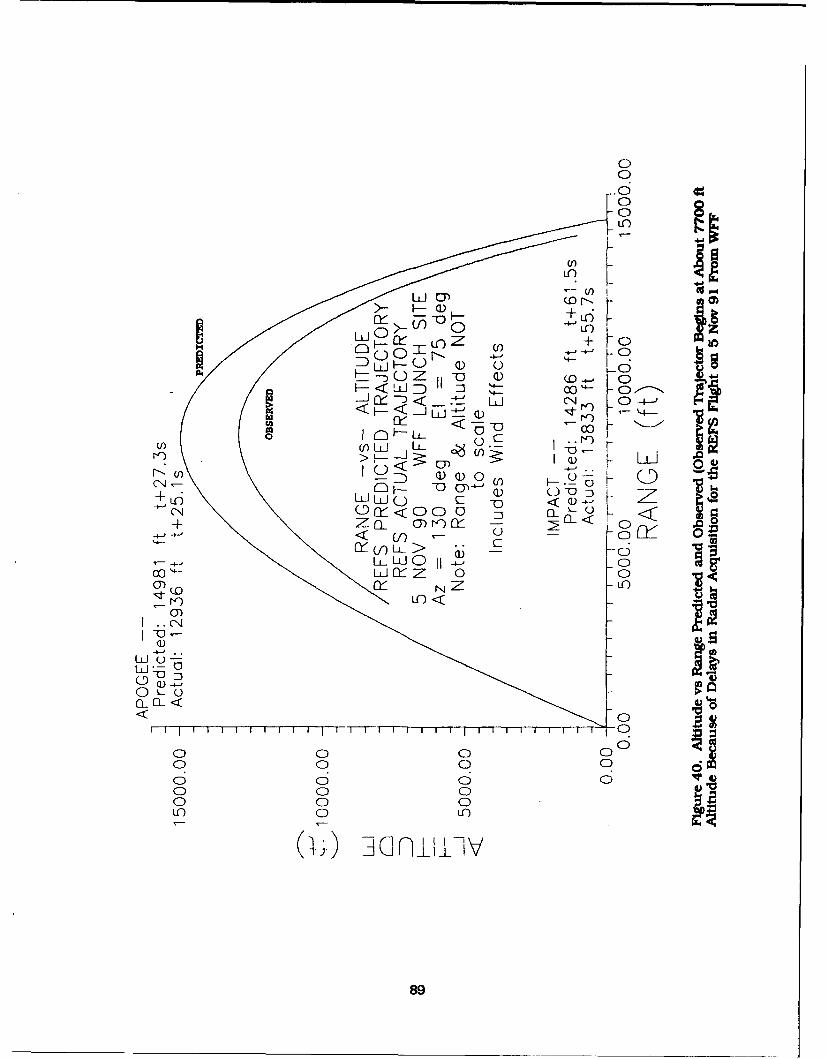
0

LLJ 0)

_y -ii-

7- U

<2 -.L 00'- D< [--J 4 -4- 0o (

I <

LC) 0

89<0

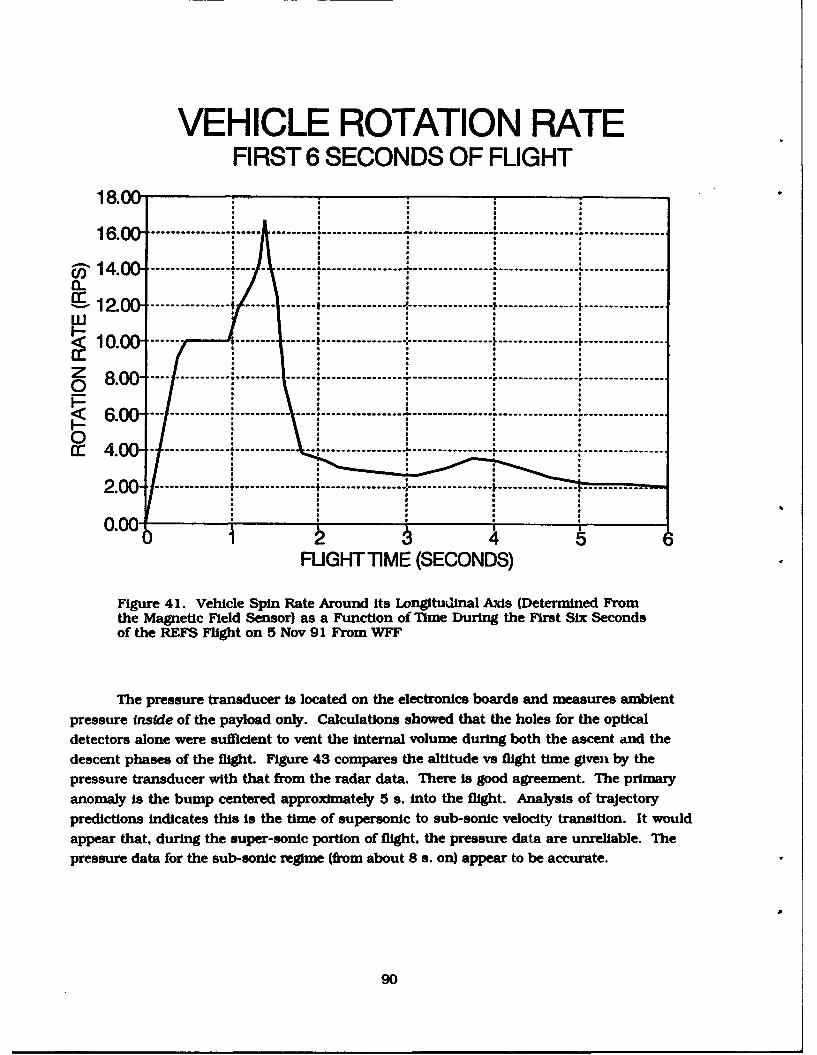
VEHICLE ROTATION RATEFIRST 6 SECONDS OF FLIGHT

18.00 -16 0 ............. ----- ....... . ................... * ---------

U---------------------------------- ------ --------------- ---------------- ---------------------------------

------------------ ...... ..... ------------------ ---- ----- --------

W:

016.00 .- ... . .-----

---------------- ---------------

14

14.00 - --- ------------------------- .....- .................. - - ---- ---------------- -----------------

2.00 ---------------- *i--------------- ----------------04 ----------- ---- -------------

0.00-4 6

FUGHT TIME (SECONDS)

Figure 41. Vehicle Spin Rate Around Its Longitudinal Axis (Determined Fromthe Magnetic Field Sensor) as a Function of Time During the First Six Secondsof the REFS Flight on 5 Nov 91 From WFF

The pressure transducer is located on the electronics boards and measures ambient

pressure inside of the payload only. Calculations showed that the holes for the optical

detectors alone were sufficient to vent the internal volume during both the ascent and the

descent phases of the flight. Figure 43 compares the altitude vs flight time given by the

pressure transducer with that from the radar data. There is good agreement. The primary

anomaly is the bump centered approximately 5 s. into the flight. Analysis of trajectory

predictions indicates this Is the time of supersonic to sub-sonic velocity transition. It would

appear that, during the super-sonic portion of flight, the pressure data are unreliable. The

pressure data for the sub-sonic regime (from about 8 s. on) appear to be accurate.

90

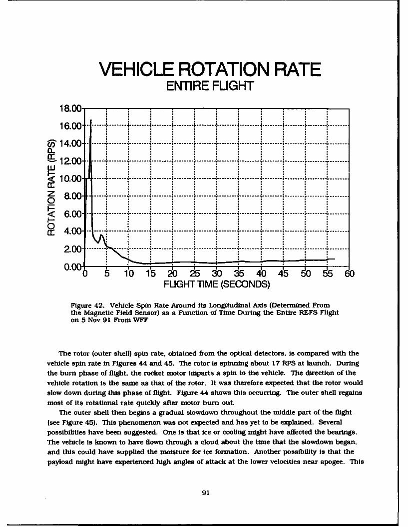
VEHICLE ROTATION RATEENTIRE FUGHT

18.00-16.00 . ..... -------- ........ - -------- - -- -------- . -...... --------. - I ----------

"14.00 - --.. ..................---............. -..------.--S14.00. .. ........................ ................ , .. . . . . . .

10.00 ....-..................................................

*8 . ............. r -------- w ........ - I • -... ............... -....... ......

.00................................ -...... . ..........................................

4.00-"Z"8---4........................."

2.00...... 65 -. I........ -......

0.0 oo -- 1 '0 115 ý6 5 ýo 5 ~5 0 ý5 EbFUGHT TIME (SECONDS)

Figure 42. Vehicle Spin Rate Around its Longitudinal Axis (Determined Fromthe Magnetic Field Sensor) as a Function of Time During the Entire REFS Flighton 5 Nov 91 From WFF

The rotor (outer shell) spin rate, obtained from the optical detectors, is compared with the

vehicle spin rate in Figures 44 and 45. The rotor is spinning about 17 RPS at launch. During

the burn phase of flight, the rocket motor imparts a spin to the vehicle. The direction of the

vehicle rotation is the same as that of the rotor. It was therefore expected that the rotor would

slow down during this phase of flight. Figure 44 shows this occurring. The outer shell regains

most of its rotational rate quickly after motor burn out.

The outer shell then begins a gradual slowdown throughout the middle part of the flight

(see Figure 45). This phenomenon was not expected and has yet to be explained. Several

possibilities have been suggested. One is that ice or cooling might have affected the bearings.

The vehicle is known to have flown through a cloud about the time that the slowdown began.

and this could have supplied the moisture for ice formation. Another possibility is that the

payload might have experienced high angles of attack at the lower velocities near apogee. This

91

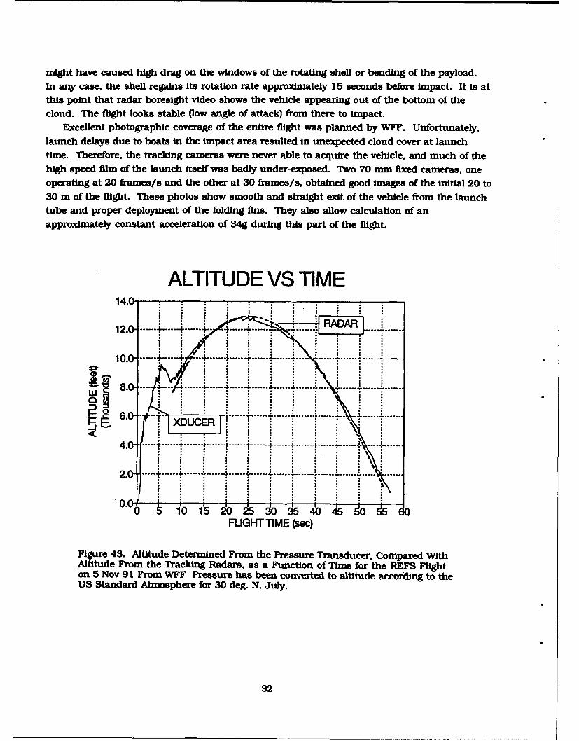
might have caused high drag on the windows of the rotating shell or bending of the payload.In any case, the shell regains its rotation rate approximately 15 seconds before impact. It is atthis point that radar boresight video shows the vehicle appearing out of the bottom of thecloud. The flight looks stable (low angle of attack) from there to impact.

Excellent photographic coverage of the entire flight was planned by WFF. Unfortunately,launch delays due to boats in the impact area resulted in unexpected cloud cover at launchtime. Therefore, the tracking cameras were never able to acquire the vehicle, and much of thehigh speed film of the launch itself was badly under-exposed. Two 70 mm fixed cameras, oneoperating at 20 frames/s and the other at 30 frames/s. obtained good Images of the initial 20 to30 m of the flight. These photos show smooth and straight exit of the vehicle from the launchtube and proper deployment of the folding fins. They also allow calculation of anapproximately constant acceleration of 34g during this part of the flight.

ALTITUDE VS TIME14.01 1 O 5 d d

1 2 .0 " . .. ........ . . . . .,. .. .. .. . . ..... . .......

10.0 . ....... L.... I .. ............... : "....... L. . ...... ". ... "... .-

8 0 -- ...... . ...... .4 .......

W 4 .0 - . . .. ..... .+ . .... --- --- ....... T . . .+ .. . .+ ..... T ....... )..... .-------- •- .... --. . ..

2.0 ......... .....---.............-........ ................ . .......... ---- ....... l .....: ......

FUGHT TIME (sec)

Figure 43. Altitude Determined From the Pressure Transducer, Compared WithAltitude From the Tracking Radars, as a Function of Time for the REFS Flighton 5 Nov 91 From WFF Pressure has been converted to altitude according to theUS Standard Atmosphere for 30 deg. N. July.

92

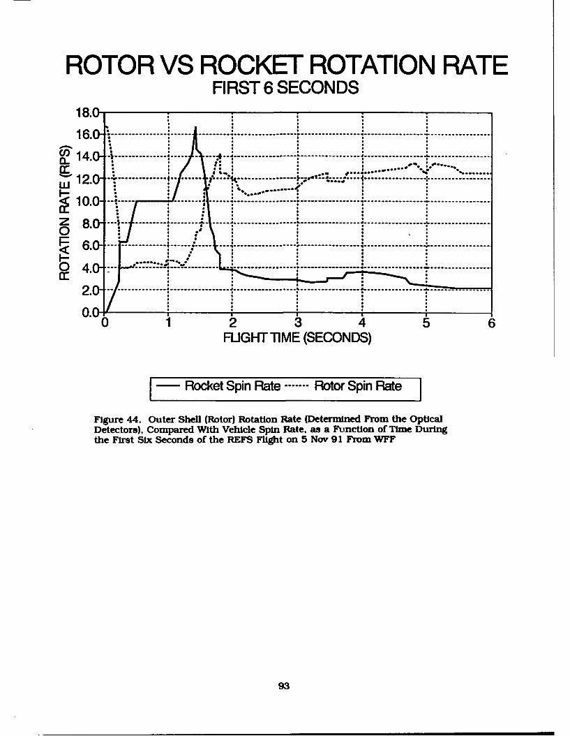
ROTOR VS ROCKET ROTATION RATEFIRST 6 SECONDS

18.0- ,

16.0-c .. .. ..... . .. ... . ... .•....

u ) 1 2 .0 - .... .... .......----- ................ .. . -- ----.. . . . . . . . . .. . . .-- --------................... . .-

10.0 8 -- - - ------ .....--------------------------------- J

uJ 12 0 "• ........ :"# ......... :-" :'..'": :* -- :. :::100 " ! : . ..

- --------- ---0--- ------ I ------------------ . -----------------

Z 8 -- ------0

0 4.:- .. .... •°....,•...L........ . ...... ... .. ....... ......... •.... ......................... . .................

2.0 ------ -------- --- ----------- -- ---- ----- ---- --- - -- ------ -

0.0-06

FUGHT TIME (SECONDS)

. - Rocket Spin Rate....Rotor Spin Rate

Figure 44. Outer Shell (Rotor) Rotation Rate (Determined From the OpticalDetectors), Compared With Vehicle Spin Rate, as a Function of Time Duringthe First Six Seconds of the REFS Flight on 5 Nov 91 From WFF

93

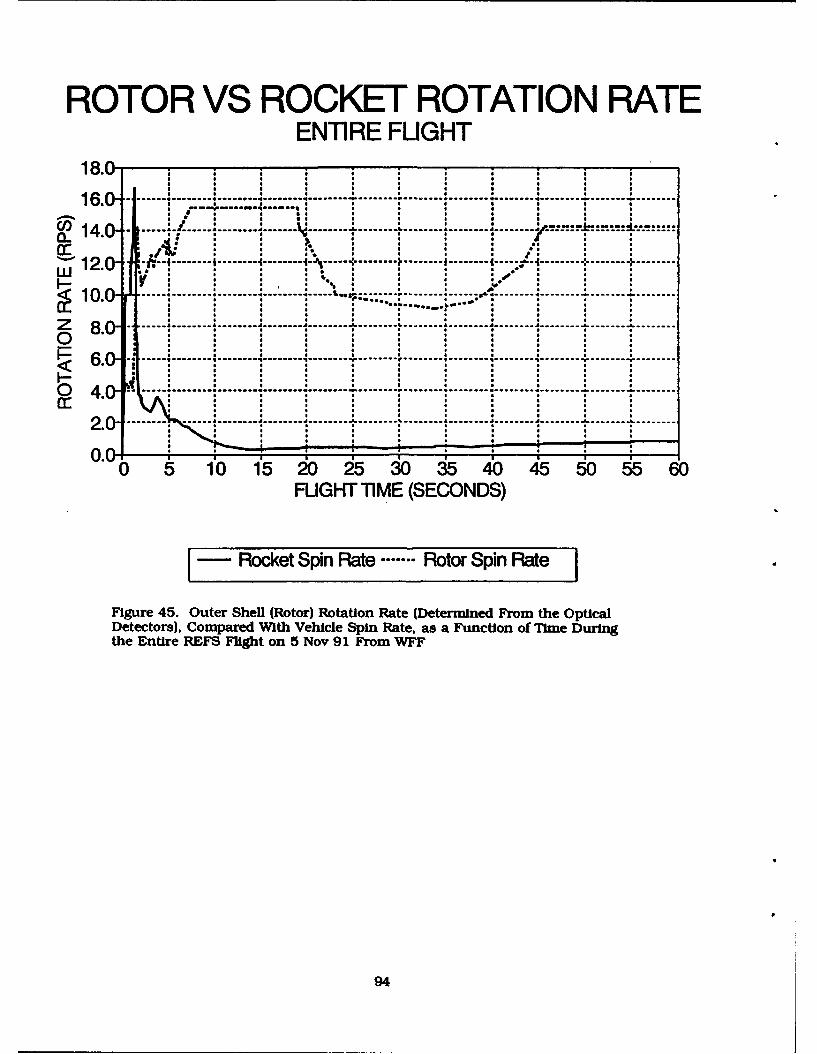
ROTOR VS ROCKET ROTATION RATEENTIRE FLIGHT

18.0-

16.0- .........-...... .... . ..... ...........

1_ . . ...-- ----... --S* S S a d/o flo

- --12.0- -t.......... .................. i , '. e.. -. -------- -.......10 fl.i*sS*........ ,........ •......i4 ........8 I0 0 .... .... ...... .................. ..... ....

S60.------

40-J.. . .. ........... ................ I................. ............................................--

2. - ------0.0 i__ _- a I __ __ I ___ I _ __ __ __ _

0 5 10 15 20 25 30 35 40 45 50 55 60

FUGHT TIME (SECONDS)

Rocket Spin Rate ....... Rotor Spin Rate

Figure 45. Outer Shell (Rotor) Rotation Rate (Determined From the OpticalDetectors), Compared With Vehicle Spin Rate, as a Function of Time Duringthe Entire REFS Flight on 5 Nov 91 From WFF

94

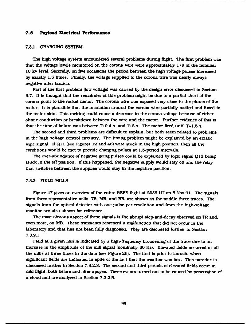
7.8 Payload Electrical Performance

7.3.1 CHARGING SYSTEM

The high voltage system encountered several problems during flight. The first problem wasthat the voltage levels monitored on the corona wire were approximately 1/8 of the nominal10 kV level. Secondly, on five occasions the period between the high voltage pulses Increasedby exactly 1.5 times.- Finally, the voltage supplied to the corona wire was nearly always

negative after launch.Part of the first problem {low voltage) was caused by the design error discussed in Section

3.7. It is thought that the remainder of this problem might be due to a partial short of thecorona point to the- rocket motor. The corona wire was exposed very close to the plume of themotor. It Is plausible that the insulation around the corona wire partially melted and fused tothe motor skin. This melting could cause a decrease in the corona voltage because of eitherohmic conduction or breakdown between the wire and the motor. Further evidence of this isthat the time of failure was between T+0.4 s. and T+2 s. The motor fired until T+1.5 s.

The second and third problems are difficult to explain, but both seem related to problemsin the high voltage control circuitry. The timing problem might be explained by an erraticlogic signal. If Q11 (see Figures 12 and 46) were stuck in the high position, then all theconditions would be met to provide charging pulses at 1.5-period intervals.

The over-abundance of negative going pulses could be explained by logic signal Q12 beingstuck in the off position. If this happened, the negative supply would stay on and the relaythat switches between the supplies would stay in the negative position.

7.3.2 FIELD MILLS

Figure 47 gives an overview of the entire REFS flight at 2036 UT on 5 Nov 91. The signalsfrom three representative mills, TR. MB, and BR, are shown as the middle three traces. Thesignals from the optical detector with one pulse per revolution and from the high-voltagemonitor are also shown for reference.

The most obvious aspect of these signals is the abrupt step-and-decay observed on TR and.even more, on MB. These transients represent a malfunction that did not occur in thelaboratory and that has not been fully diagnosed. They are discussed further in Section7.3.2.1.

Field at a given mill is Indicated by a high-frequency broadening of the trace due to anincrease in the amplitude of the mill signal (nominally 30 Hz). Elevated fields occurred at allthe mills at three times in the data (see Figure 26). The first is prior to launch, whensignificant fields are indicated in spite of the fact that the weather was fair. This paradox isdiscussed further in Section 7.3.2.3. The second and third periods of elevated fields occur inmid flight, both before and after apogee. These events turned out to be caused by penetration ofa cloud and are analyzed in Section 7.3.2.5.

95

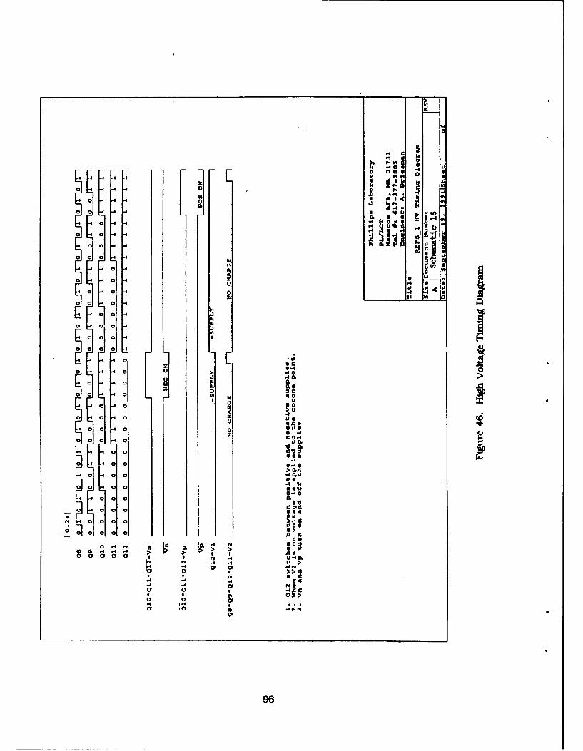
0

.41 f 0 .4 a

0 000,

0 0 I4 .ý 44 -

a. 0

00 0 l F

00 0 -%-

000 (0

0 0 4000

U .- 4 N 6

00 0 -

0 a00

0 0 0

0 0 i 0.z 0 0.4

00 0 -40'4 a 4

0 00a

z~ 0.4

-44

0 0 0 06*04

N 0 0 0 .- 4 C

40 0

c14CI

0N -4 - IC IC6

-4 . . 40 4~ > I I C >

0 0.4 C

ol 0 a6

964A

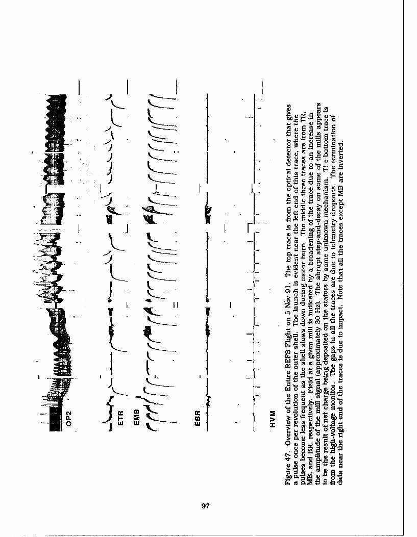
"•~ "-0-. 0u -'

0 tot

0 0

I ,_ Cu •. F_ .

-4 L• '-o .

" -.. • Ow -, :1

. 5 - -

t ... ca ,• •o ,,,:•

t• o ,0 bc.

) .--- I€ £-v- I: •

Ia '

Mr-:-.I• I 0, .4U , N

R I 0, =- '

0Cu-IOU

97

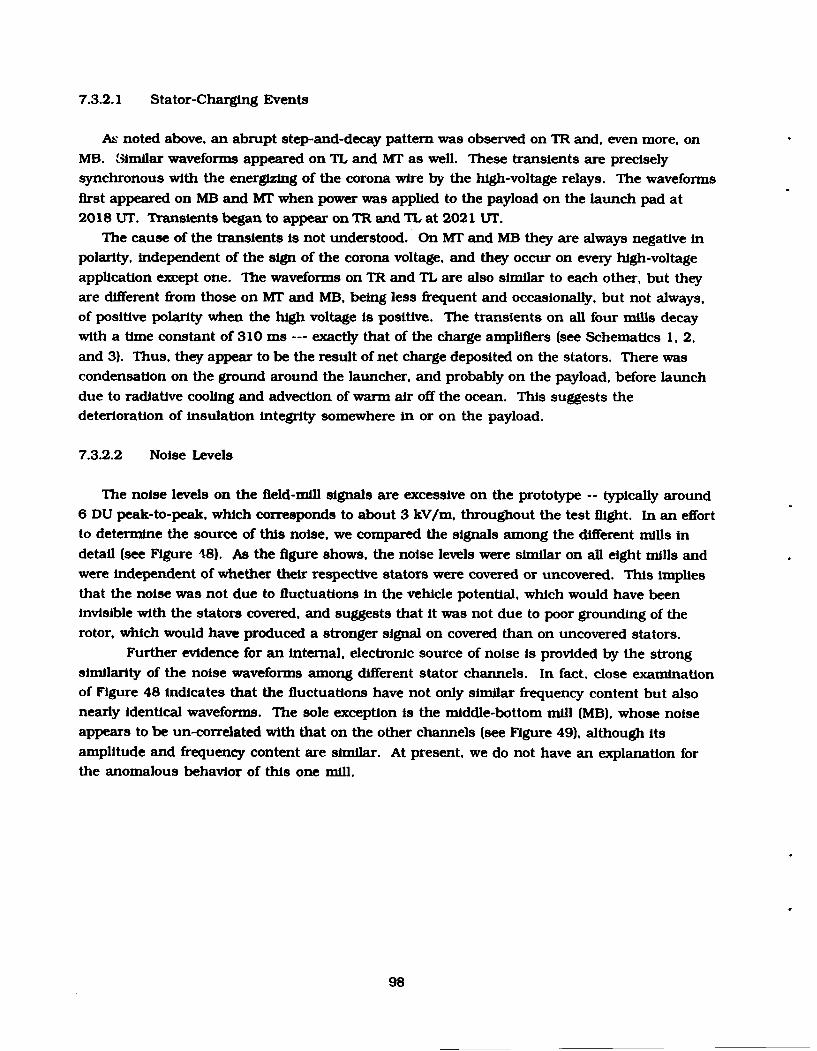
7.3.2.1 Stator-Charging Events

As noted above, an abrupt step-and-decay pattern was observed on TR and, even more, onMB. Similar waveforms appeared on TL and MT as well. These transients are precisely

synchronous with the energizing of the corona wire by the high-voltage relays. The waveforms

first appeared on MB and MT when power was applied to the payload on the launch pad at2018 UT. Transients began to appear on TR and TL at 2021 UT.

The cause of the transients is not understood. On MT and MB they are always negative in

polarity, independent of the sign of the corona voltage, and they occur on every high-voltage

application except one. The waveforms on TR and TL are also similar to each other, but theyare different from those on MT and MB, being less frequent and occasionally, but not always,

of positive polarity when the high voltage is positive. The transients on all four mills decaywith a time constant of 310 ms --- exactly that of the charge amplifiers (see Schematics 1, 2,

and 3). Thus, they appear to be the result of net charge deposited on the stators. There wascondensation on the ground around the launcher, and probably on the payload, before launch

due to radiative cooling and advection of warm air off the ocean. This suggests thedeterioration of insulation integrity somewhere in or on the payload.

7.3.2.2 Noise Levels

The noise levels on the field-mill signals are excessive on the prototype -- typically around

6 DU peak-to-peak, which corresponds to about 3 kV/m, throughout the test flight. In an effort

to determine the source of this noise, we compared the signals among the different mills in

detail (see Figure 18). As the figure shows, the noise levels were similar on all eight mills andwere independent of whether their respective stators were covered or uncovered. This implies

that the noise was not due to fluctuations in the vehicle potential. which would have beeninvisible with the stators covered, and suggests that it was not due to poor grounding of the

rotor, which would have produced a stronger signal on covered than on uncovered stators.Further evidence for an internal, electronic source of noise is provided by the strong

similarity of the noise waveforms among different stator channels. In fact, close examinationof Figure 48 indicates that the fluctuations have not only similar frequency content but also

nearly identical waveforms. The sole exception is the middle-bottom mill (MB), whose noiseappears to be un-correlated with that on the other channels (see Figure 49), although its

amplitude and frequency content are similar. At present, we do not have an explanation forthe anomalous behavior of this one mill.

98

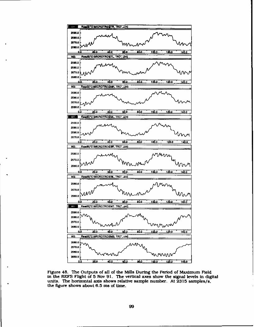
M.~edUIOMMICROTMOITIF. TRO". ulflt

2M0.0

2070.0

2100.0-

2090.0 J2080.0

2070.0

WI: R&WdB(CAPAICROTAC\EBR. TRC., LiIt

2070.0

W2: AWaB('C.\MICROTRC\EWB. TAG' IIInt

Fiue 8 TeOuptso alofte ilsDrigth1ero0o0ax.m0ilInte ES lgh f5 o 9.Th eria ae 2o0tesinllees.ndiiaunt. h hrzotl xs hwsrlaie apl2ume.8t235sapessthe~~~07. fiuesosaot65-so ie

[-- 0. 2.0 4d0 .6o 6. 13. 1b.991z

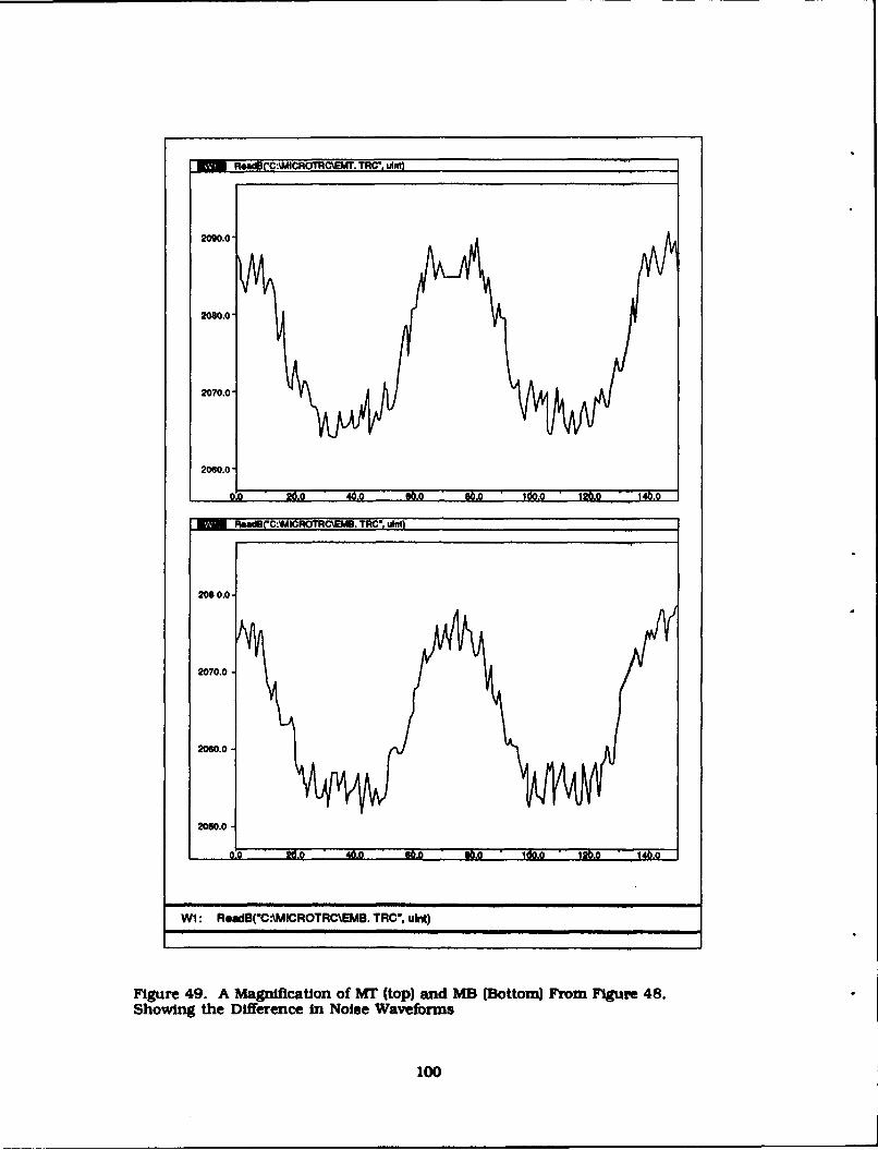
RemdB C.•ICROTCREMI. TRC*" lAnt)

2090.0-

2W.0"

2070.0-

2 0 6 0 .0 0

, ReOMBC:MWAICROTRC•MI. T0C". uLnt)

208 0.0-

2070.0-

2060.0

2050.0-

WI: ReadB(C-\MICROTRC\EMB. TRC', urlt)

FIgure 49. A Magifi•cation of Mr (top) and MB (Bottom) From Flgure 48,

Showing the Difference in Noise Waveforms

100

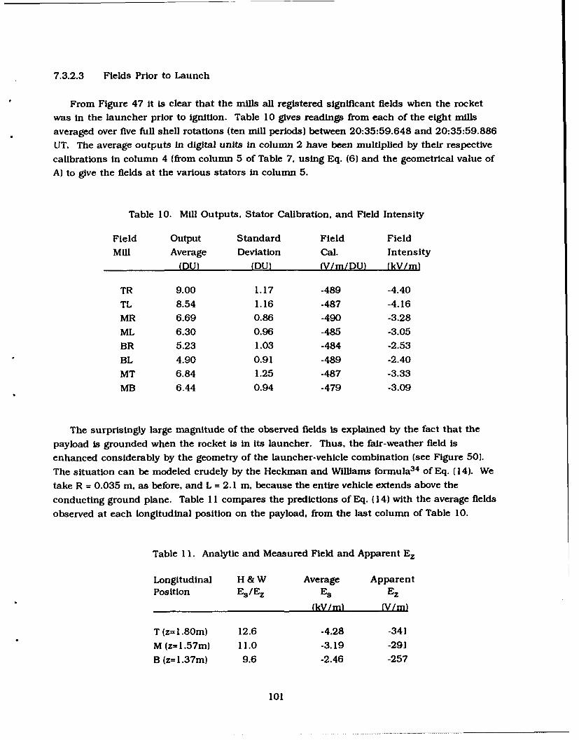
7.3.2.3 Fields Prior to Launch

From Figure 47 it is clear that the mills all registered significant fields when the rocket

was in the launcher prior to ignition. Table 10 gives readings from each of the eight mills

averaged over five full shell rotations (ten mill periods) between 20:35:59.648 and 20:35:59.886

UT. The average outputs in digital units in column 2 have been multiplied by their respective

calibrations in column 4 (from column 5 of Table 7. using Eq. (6) and the geometrical value of

A) to give the fields at the various stators in column 5.

Table 10. Mill Outputs. Stator Calibration, and Field Intensity

Field Output Standard Field Field

Mill Average Deviation Cal. Intensity

(DU) (DU) (V/m/DU) 1kV/m)

TR 9.00 1.17 -489 -4.40

TL 8.54 1.16 -487 -4.16

MR 6.69 0.86 -490 -3.28

ML 6.30 0.96 -485 -3.05

BR 5.23 1.03 -484 -2.53

BL 4.90 0.91 -489 -2.40

MT 6.84 1.25 -487 -3.33

MB 6.44 0.94 -479 -3.09

The surprisingly large magnitude of the observed fields Is explained by the fact that the

payload is grounded when the rocket is in its launcher. Thus, the fair-weather field is

enhanced considerably by the geometry of the launcher-vehicle combination (see Figure 50).

The situation can be modeled crudely by the Heckman and Williams formula 3 4 of Eq. (14). We

take R = 0.035 m, as before, and L = 2.1 m, because the entire vehicle extends above the

conducting ground plane. Table I 1 compares the predictions of Eq. 14) with the average fields

observed at each longitudinal position on the payload, from the last column of Table 10.

Table 11. Analytic and Measured Field and Apparent Ez

Longitudinal H & W Average ApparentPosition Es/Ez Es Ez

WkV/ml (V/m)

T (z= 1.80m) 12.6 -4.28 -341

M (z=l.57m) 11.0 -3.19 -291

B (z=1.37m) 9.6 -2.46 -257

101

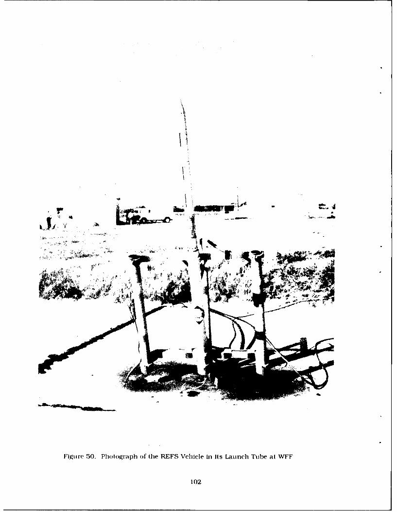
- tirb~~'Ž -1n

I 4"-44'All

Figure 50. Photograph of the REFS Vehicle in Its Launch Tube at WVFF

102

One may obtain rough estimates of the ambient vertical field (column 4) by dividing themeasured fields in column 3 by the Heckman and Williams field-enhancement factors incolumn 2. These estimates are as consistent from position to position as can be expected inview of the complex geometry of Figure 50 and the approximations involved in Eq. (14).Although they are large for fair-weather fields, they are entirely reasonable for fields

downwind from a salt-water surf zone. 35 The launch site was Just tens of meters from theAtlantic Ocean, and the wind was on shore at launch time.

7.3.2.4 Response to Charging System

The response of the vehicle potential to corona pulses from the charging system was less

than satisfactory. At the lowered voltages measured on the corona wire during flight, the fewpositive-polarity pulses that occurred had little effect. (The last "full voltage" pulse of about 4.6kV was positive, but it occurred during motor burn so that its result was ambiguous.) Negative-polarity corona pulses generally had a noticeable effect, especially toward the end of the flight.

One example is reproduced in Figure 51, which shows positive fields appearing on arepresentative set of mills during the high-voltage pulse and lasting for a few hundredmilliseconds thereafter. Although the magnitude of the fields measured during these eventswas too small to read accurately, they were consistent with the expectation that positive chargewas deposited on the rocket.

It was observed that the field always decayed away in a fraction of a second after the highvoltage was turned off. This was not expected, since the conductivity of air is extremely low. Itis assumed that net charge on the vehicle was carried away by smoke emerging from the rocket

motor after burnout.

7.3.2.5 In-Flight Potential Calibration

Since the first flight of REFS occurred during fair weather, there were no measurable

ambient fields with which to test the accuracy of the matrix coefficients in Eq. (15) or tocalibrate the longitudinal component of the field. As noted above, artificial charging from theinternal high-voltage supplies was also too weak during this flight to allow accurate

calibration of the mills' potential coefficients. Fortunately, the vehicle passed through a thinaltocumulus layer at about 13,000 ft altitude both before and after apogee (see Figure 47). Cloud

penetration was indicated by reduced variation of the optical-detector amplitude with rocketrotation (as deduced from the magnetic detector). During both of these cloud penetrations, allthe field mills indicated significant local fields due to charging of the vehicle by particleimpaction. The largest fields were recorded at about 20:36:36.5 UT, on the ascending leg. whenthe various mills registered between -17 and -20 kV/m at the surface of the payload.

z Gathman, S.G., and Hoppel, WA. (1970) Surf electrification, J. Geophys. Res., 75:4525-4529.

103

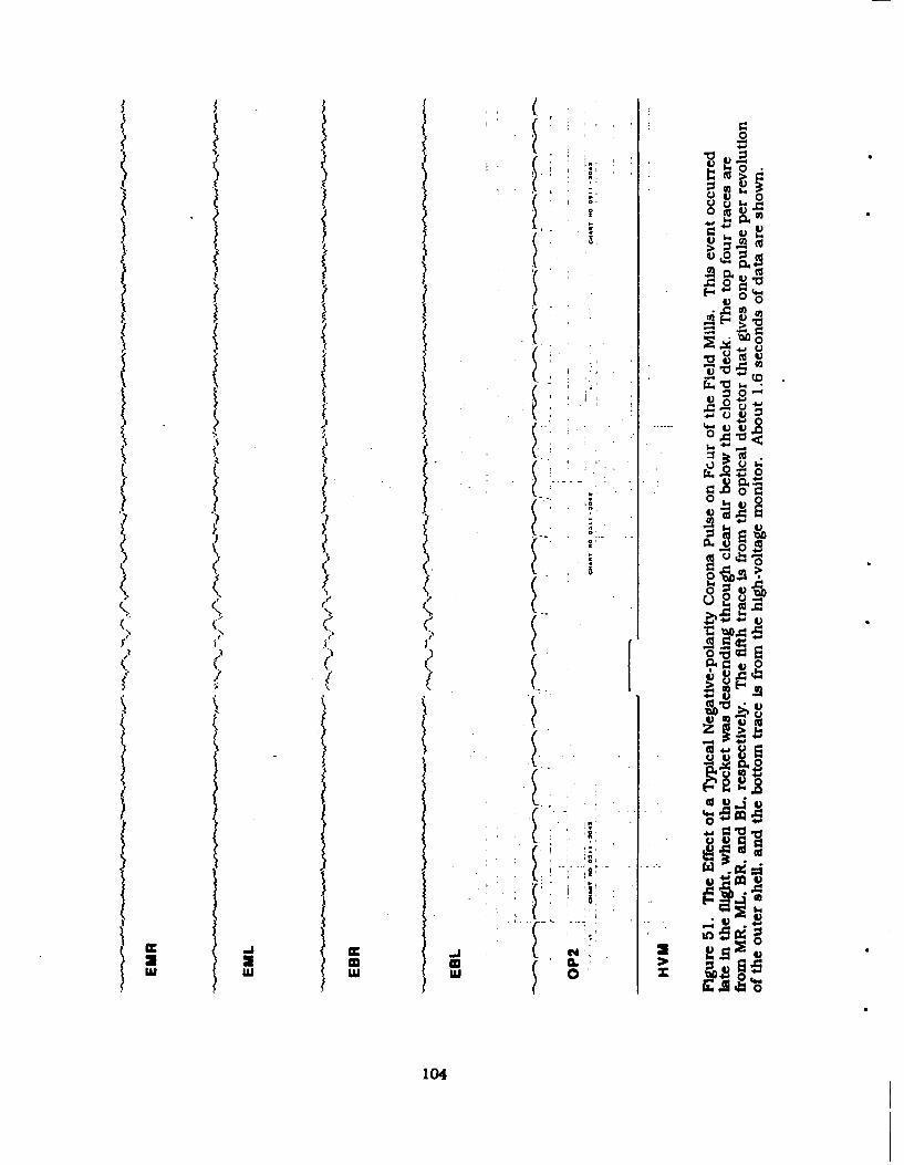
4.J

$ýV~~~ 0*~(U*

I'v3'or-

( Cj, '(L -0 ow

r.O

cc .5 cc 2 4)0

a a(I (A w

K 104

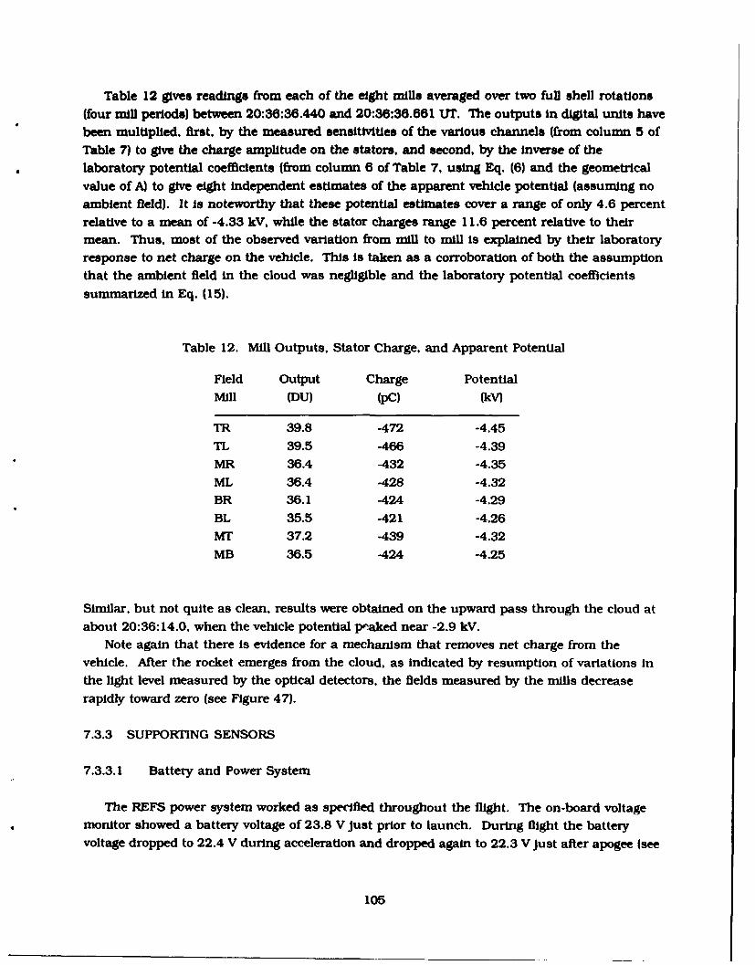
Table 12 gives readings from each of the eight mills averaged over two full shell rotations(four mill periods) between 20:36:36.440 and 20:36:36.661 UT. The outputs in digital units havebeen multiplied, first, by the measured sensitivities of the various channels (from column 5 ofTable 7) to give the charge amplitude on the stators, and second, by the Inverse of thelaboratory potential coefficients (from column 6 of Table 7, using Eq. (6) and the geometricalvalue of A) to give eight independent estimates of the apparent vehicle potential (assuming noambient field). It is noteworthy that these potential estimates cover a range of only 4.6 percentrelative to a mean of -4.33 kV, while the stator charges range 11.6 percent relative to theirmean. Thus, most of the observed variation from mill to mill is explained by their laboratoryresponse to net charge on the vehicle. This is taken as a corroboration of both the assumptionthat the ambient field in the cloud was negligible and the laboratory potential coefficientssummarized in Eq. (15).

Table 12. Mill Outputs, Stator Charge, and Apparent PotenUal

Field Output Charge PotentialMill (DU) (pC) (WV

TR 39.8 -472 -4.45

TL 39.5 -466 -4.39MR 36.4 -432 -4.35ML 36.4 -428 -4.32BR 36.1 -424 -4.29BL 35.5 -421 -4.26MT 37.2 -439 -4.32MB 36.5 -424 -4.25

Similar, but not quite as clean, results were obtained on the upward pass through the cloud atabout 20:36:14.0. when the vehicle potential peaked near -2.9 kV.

Note again that there Is evidence for a mechanism that removes net charge from thevehicle. After the rocket emerges from the cloud, as indicated by resumption of variations inthe light level measured by the optical detectors, the fields measured by the mills decreaserapidly toward zero (see Figure 47).

7.3.3 SUPPORTING SENSORS

7.3.3.1 Battery and Power System

The REFS power system worked as specified throughout the flight. The on-board voltagemonitor showed a battery voltage of 23.8 V Just prior to launch. During flight the batteryvoltage dropped to 22.4 V during acceleration and dropped again to 22.3 V Just after apogee (see

105

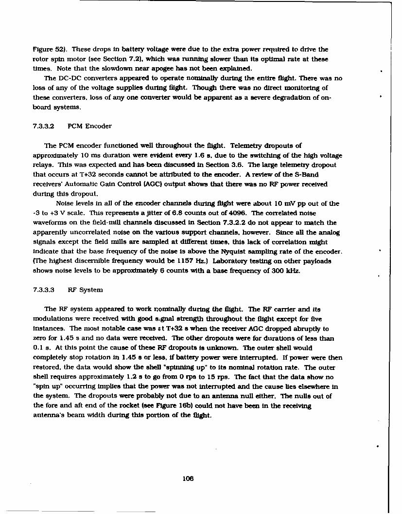
Figure 52). These drops in battery voltage were due to the extra power required to drive therotor spin motor (see Section 7.2), which was running slower than its optimal rate at thesetimes. Note that the slowdown near apogee has not been explained.

The DC-DC converters appeared to operate nominally during the entire flight. There was noloss of any of the voltage supplies during flight. Though there was no direct monitoring ofthese converters, loss of any one converter would be apparent as a severe degradation of on-board systems.

7.3.3.2 PCM Encoder

The PCM encoder functioned well throughout the flight. Telemetry dropouts ofapproximately 10 ms duration were evident every 1.6 s. due to the switching of the high voltagerelays. This was expected and has been discussed in Section 3.6. The large telemetry dropoutthat occurs at T+32 seconds cannot be attributed to the encoder. A review of the S-Bandreceivers' Automatic Gain Control (AGC) output shows that there was no RF power receivedduring this dropout.

Noise levels in all of the encoder channels during flight were about 10 mV pp out of the-3 to +3 V scale. This represents a Jitter of 6.8 counts out of 4096. The correlated noisewaveforms on the field-mill channels discussed in Section 7.3.2.2 do not appear to match the

apparently uncorrelated noise on the various support channels, however. Since all the analogsignals except the field mills are sampled at different times, this lack of correlation mightIndicate that the base frequency of the noise is above the Nyquist sampling rate of the encoder.

(The highest discernible frequency would be 1157 Hz.) Laboratory testing on other payloadsshows noise levels to be approximately 6 counts with a base frequency of 300 kHz.

7.3.3.3 RF System

The RF system appeared to work nominally during the flight. The RF carrier and Itsmodulations were received with good signal strength throughout the flight except for fiveinstances. The most notable case was ,t T+32 s when the receiver AGC dropped abruptly tozero for 1.45 s and no data were received. The other dropouts were for durations of less than0.1 s. At this point the cause of these RF dropouts is unknown. The outer shell wouldcompletely stop rotation in 1.45 s or less, if battery power were interrupted. If power were thenrestored, the data would show the shell "spinning up" to its nominal rotation rate. The outershell requires approximately 1.2 s to go from 0 rps to 15 rps. The fact that the data show no"spin up" occurring implies that the power was not interrupted and the cause lies elsewhere inthe system. The dropouts were probably not due to an antenna null either. The nulls out ofthe fore and aft end of the rocket (see Figure 16b) could not have been in the receivingantenna's beam width during this portion of the flight.

106

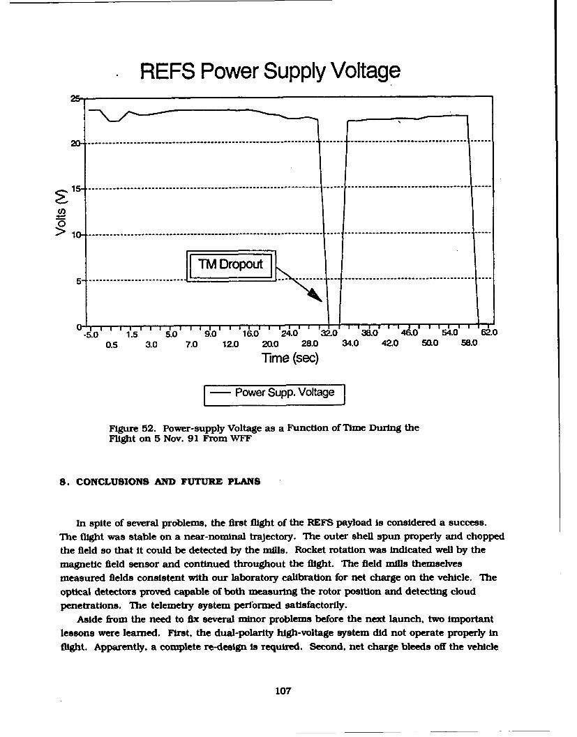
REFS Power Supply Voltage

. - -------------......--...-.- ---.....o°...°°o ...... .......

S s---------------------------------- ---------------------------------- --

10------------------------------------------------------------------------ ----

ITM Dropout5 ------------------- ......... --------------------.... -------- ----

-5.0 1.5 5.0 9.0 16.0 24.0 32._0 38.0 46.0 54.0 62.00.5 ao 7.0 12.0 200 28.0 34.0 42.0 50.0 58.0

"Time (sec)

- Power Supp. Voltage

Figure 52. Power-supply Voltage as a Function of Time During theFlight on 5 Nov. 91 From WFF

8. CONCLUSIONS AND FUTURE PLANS

In spite of several problems, the first flight of the REFS payload is considered a success.

The flight was stable on a near-nominal trajectory. The outer shell spun properly and chopped

the field so that it could be detected by the mills. Rocket rotation was indicated well by themagnetic field sensor and continued throughout the flight. The field mills themselves

measured fields consistent with our laboratory calibration for net charge on the vehicle. The

optical detectors proved capable of both measuring the rotor position and detecting cloudpenetrations. The telemetry system performed satisfactorily.

Aside from the need to fix several minor problems before the next launch, two important

lessons were learned. First, the dual-polarity high-voltage system did not operate properly inflight. Apparently, a complete re-design Is required. Second. net charge bleeds off the vehicle

107

very rapidly in flight. This eliminates the need, discussed in Section 2.2. for a dual-polarity

supply. Therefore, the next generation of REFS will have only a single high-voltage supply

that will be directly connected to the corona emitter. A major advantage of this design

simplification is the elimination of the high-voltage relays, which failed to perform as

expected.

In an effort to further increase the efficiency and reliability of the corona-charging system,

the emitter has been re-designed as illustrated in Figure 53. This assembly is to be slid over

the motor shell and glued in place near the aft end, eliminating the insulated wire trailing

near the exhaust plume. Four corona points (as opposed to the single point in the first launch)

will spring out when the rocket leaves the launch tube. They will be oriented so as to produce

plumes of ions that are carried between the fins and away from the vehicle by the rocket's

motion through the air.

The next step in the development of REFS is to carry out some flights in high fields, thick

clouds, and precipitation. Three more launches were planned for August, 1991, at KSC to test

the modified design and verify proper performance under thunderstorm conditions.

Unfortunately, unfavorable weather and ordnance-safety issues prevented these launches,

which are now planned for July 1992.

108

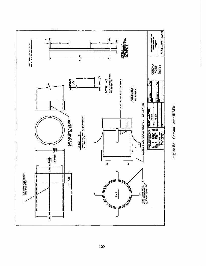
oP-

I II-. U -J00-

i 1 - "4 *

ii

109

el g LE

100

References

1. NASA Goddard Space Flight Center (1987) Atlas/Centaur-67 FLTSATCOM F-6 InvestigationBoard, Report, NASA Goddard Space Flight Center, Greenbelt. MD 20771, 15 July 1987.

2. Mazur, V., Fisher, B.D., and Gerlach, J.C. (1984) Uightning Strikes to an airplane in athunderstorm, J. Aircraft, 21:607-611.

3. Boulay, J.L., Moreau, J.P., Asselineau, A., and Rustan, P.L. (1988) Analysis of recent in-flight lightning measurements on different aircraft, paper presented at theInternational Aerospace and Ground Conference on Lightning and Static Electricity,National Oceanic and Atmospheric Administration, Oklahoma City, OK.

4. Heritage, H., (1988) Launch vehicle llghtning/atmospherlc electrical constraints post-Atlas/Centaur 67 incident, Report No. TOR-0088(3441-45)-2, The Aerospace Corporation.El Segundo, CA 90245.

5. Bailey, J.. Mach, D.M., and Christian, H.J. (1990) In flight vector calibration of shutter typefield mills aboard a Lear 28/29 aircraft, presented at the Fall Annual Meeting of theAmerican Geophysical Union, Dec. 4, 1990, San Francisco, CA.

6. Mach, D.M., and Christian, H.J. (1990) Initial electrification of a Florida cumulus,presented at the Fall Annual Meeting of the American Geophysical Union, Dec. 4, 1990,San Francisco, CA.

7. Fleux, R.P., Gary, C.H., Hutzler, B.P., Eybert-Berard, A.R., Hubert. P.L., Meesters, A.C.,Perroud, P.H., Hamelin, J.H., and Person, J.M. (1978) Research on artificially triggeredlightning In France, IEEE Trans. Power Appar. Syst., PAS-97:725-733.

8. Laroche, P., Eybert-Berard, A., and Barret, L. (1985) Triggered lightning flashcharacterization, in Tenth International Aerospace and Ground Conference on Lightningand Static Electricity (ICOLSE), Paris, pp.231-239, Les Editions de Physique, Les Ulis.France.

111

9. Leteinturier, C., Weidman, C., and Hamelin, J. (1990) Current and electric field derivativesin triggered lightning return strokes, J. Geophys. Res., 95:811-828.

10. Idone, V.P., Orville, R.E., Hubert. P., Barret, L., and Eybert-Berard, A. (1984) Correlatedobservations of three triggered lightning flashes, J. Geophys. Res., 89:1385-1394.

11. Laroche, P., Boudiou, A., Eybert-Berard, A.. Barret, L., Berlandis, J.P., Terrier, G., andJafferis, W. (1989) Lightning flashes triggered in altitude by the rocket and wiretechnique, paper presented at the International Conference on Lightning and StaticElectricity, Ministry of Defense Procurement Executive, U.K., Bath, England, Sept.,1989.

12. Mazur, V., t1988) Lightning initiation on aircraft in thunderstorms, paper presented at the26th AIAA Meeting, Reno, NV, Jan.

13. Jackson, J.D., (1975) Classical Electrodynamics, John Wiley & Sons. New York.

14. Standler, R.B., and Winn, W.P. (1979) Effects of coronae on electric fields beneaththunderstorms, Quart J. Roy. Met. Soc., 105:285-302.

15. Thayer, J.S., Nanevics, J.E., and Glori, K.L. (1989) Triggering of lightning by launchvehicles: determination of the ambient field vehicle enhancement factors, SRIInternational. Menlo Park, CA 94025.

16. Anderson. R.V.. and Bailey, J.C. (1987) Vector electricfields measured in a lightningenvironment, Memorandum Report 5899, Naval Research Laboratory, Washington, DC20375.

17. Laroche, P., Delannoy. A., and Le Court de Beru, H. (1989) Electrostatic field conditions onan aircraft stricken by lightning, paper presented at the International Conference onLightning and Static Electricity, Ministry of Defense Procurement Executive, U.K..Bath, England, Sept.

18. Latham, D.J., (1974) Atmospheric Electrical Effects of an on Tethered Balloon Systems,Report 2176, Advanced Research Projects Agency, Arlington, Va. 22209.

19. Jonsson, H.H., (1990) Possible errors in electrical measurements made In thundercloudswith balloon-borne instrumentation, submitted to J. Geophys. Res.

20. Winn. W.P., Schwede, G.W., and Moore, C.B. (1974) Measurements of electric fields inthunderclouds, J. Geophys. Res., 79:1761-1767.

21. Ruhnke, L.H., (1971) A Rocket Borne Instrument to Measure Electric Fields Inside ElectrifiedClouds, NOAA/ERL, Boulder, CO.

22. Idone, V.P. and Orville, R.E. (1988) Channel tortuosity variation in Florida triggeredlightning, Geophys. Res. Lett., 15:645-648.

23. Laroche, P., Eybert-Berard, A., Barret, L., Berlandis, J.P. (1988) Observations of pre-liminary discharges initiating flashes triggered by the rocket and wire technique, paperpresented at the 8th International Conference on Lightning and AtmosphericElectricity, National Science Research Council, Uppsala, Sweden.

24. Kosltsky, J., Glori, K.L.. Mafflone, R.A.. Cronin, D.H., Nanevlcz, J.E., and Harris-Hobbs, R.(1991) Airborne Field Mill (ABFM) System Calibration Report, Project 1449, SRIInternational, Menlo Park, CA.

25. Jones, J.J., (1990) Electric charge acquired by airplanes penetrating thunderstorms,J. Geophys. Res., 95:16,589-16,600.

26. Bailey, J.C., and Anderson, R.V. (1987) Experimental Calibration of a Vector Electric FieldMeter Measurement System on an Aircraft, Memorandum Report 5900, Naval ResearchLaboratory, Washington. DC.

112

27. Laroche, P., (1986) Airborne measurements of electrical atmospheric field produced byconvective clouds, Rev. Phys. Appl., 21:809-815.

28. Nielsen, J.N., (1960) Missile Aerodynamics, McGraw-Hill Book Company, Inc., New York.

29. AVCO. (1974) MASS Program User's Manual, prepared for NASA Goddard Space FlightCenter, Greenbelt, MD, under Contract NAS5-23231, by AVCO Systems Division,Maryland Operations, Seabrook MD.

30. Gathman. S.G. (1968) Guarded double field meter, Rev. ScL Instnt, 39:43-1

31. Moore, C.B. (1983) Improved configurations of lightning rods and air terminals, J.Franklin Inst., 315:61-65.

32. Smythe, W.R. (1968) Static and Dynamic Electricity, Third Edition, McGraw-Hill BookCompany, New York.

33. Stratton, JA. (1941) Electromagnetic Theory, McGraw-Hill Book Company, New York.

34. Heckman. S.J., and Williams. E.R. (1989) Corona envelopes and lightning currents, J.Geophys. Res., 94:13, 287-13, 294.

35. Gathman, S.G., and Hoppel, WA. (1970) Surf electrification, J. Geophys. Res., 75:4525-4529.

113