J. C. Penney Company, Inc. Equity Valuation

and Analysis

As of June 1, 2007

Innovative Analysis Group Devon Bartholomew devon.bartholomew@gmail.com Rachael James rach_jam@yahoo.com Daniel Moody dan946@gmail.com Ana Tapia ana.tapia@ttu.edu Sherrelle Walker sherrelle_walker@hotmail.com

1

Table of Contents

Executive Summary 3

Business & Industry Analysis 8

Company Overview 8

Industry Overview 10

Five Forces Model 12

Rivalry Among Exiting Firms 12

Threat of New Entrants 18

Threat of Substitute Products 20

Bargaining Power of Buyers 22

Bargaining Power of Suppliers 25

Value Chain Analysis 28

Firm Competitive Advantage Analysis 34

Accounting Analysis 40

Key Accounting Policies 41

Potential Accounting Flexibility 47

Actual Accounting Strategy 49

Quality of Disclosure 50

Qualitative Analysis of Disclosure 51

Quantitative Analysis of Disclosure 53

Sales Manipulation Diagnostics 54

Expense Manipulation Diagnostic 62

Potential “Red Flags” 68

Coming Undone (Undo Accounting Distortions) 69

Financial Analysis, Forecast Financials, and Cost of Capital Estimation 71

Financial Analysis 71

Liquidity Analysis 71

Profitability Analysis 79

2

Capital Structure Analysis 84

IGR/SGR Analysis 88

Financial Statement Forecasting 90

Analysis of Valuations 101

Method of Comparables 101

Cost of Equity 110

Cost of Debt 111

Weighted Average Cost of Capital 112

Intrinsic Valuations 113

Discount Dividends Model 113

Free Cash Flows Model 115

Residual Income Model 117

Long Run Return on Equity Residual Income Model 120

Abnormal Earnings Growth Model 122

Credit Analysis 126

Analyst Recommendation 127

Appendix 129

Liquidity Ratios 129

Profitability Ratios 130

Capital Structure Ratios 131

Method of Comparables 132

Regression Analysis 133

Cost of Equity 143

Cost of Debt and WACC 144

Discount Dividends Model 145

Free Cash Flows Model 146

Residual Income Model 147

Abnormal Earnings Growth Model 148

Altman Z-score 149

References 150

3

Executive Summary

Investment Recommendation: Overvalued, Sell (6/1/2007) JCP - NYSE(6/1/2007): $81.99 Altman's Z-score 52 Week Range: $61.20 - $87.18 2002 2003 2004 2005 2006Revenue: $19,903 M 2.75 1.91 3.03 3.43 3.80Market Capitalization: $18.51 B Shares Outstanding: $226 M Valuation Estimates 3-month avg. Daily Trading Volume: 3,824,300 Actual Price (6/1/2007): $81.99 Percent Institutional Ownership: 89.70% Book Value Per Share: $18.99 Financial Based Valuations ROE: 28% Trailing P/E: $82.76 ROA: 9.30% Forward P/E: $75.61 P.E.G.: $42.55 Cost of Capital est. R2 Beta Ke P/B: $60.20 Estimated: P/EBITDA: $21.40 3-month 0.1913 1.1306 8.41% P/FCF: N/A* 6-month 0.1911 1.1302 8.40% EV/EBITDA: $72.17 2-year 0.1895 1.1252 8.40% 5-year 0.1886 1.1215 8.40% Intrinsic Valuations 10-year 0.1183 1.1203 8.39% Discount Dividend: $16.06 Free Cash Flows: $36.70 Published Beta: 0.58 Residual Income: $26.61 Kd(AT): 4.04% LR ROE: $15.33 WACC(BT): 8.72% WACC(AT): 7.28% AEG: $22.88 *Irrelevant due to negative cash flows

http://moneycentral.msn.com http://moneycentral.msn.com

4

Industry Analysis

In 1902, James Cash Penney opened the first J. C. Penney in the town of

Kemmerer, Wyoming under the name the Golden Rule. It has become one of

the largest department and discount retail chains in America. Its target market

consists of middle-income families who want the convenience of shopping for a

variety of goods at affordable prices without sacrificing quality. J. C. Penney

operates 1,033 department stores in 49 states and Puerto Rico as of February 3,

2007. It has also expanded to serve its consumer base by offering its products

and services via the internet and through distribution of its general merchandise

catalog.

Direct competitors of J. C. Penney include Kohl’s, Dillard’s, Stage Stores,

Inc., and Stein Mart. Existing firms compete for market share based on

economies of scale, tight cost controls, and investments in brand image. This

competition nearly eliminates any possibility of new entrants entering into the

industry. The majority of products found within this industry are similar, the

threat of substitute products is high and the switching costs for buyers are

extremely low. Many of the companies within this industry compete on price

while trying to maintain a certain level of quality in their products.

Firms within this industry try to differentiate their product lines. J. C.

Penney is a prime example of how this marketing strategy can help increase a

company’s market share within the retail industry. However, differentiation does

not come without a price. Because of the contracts and patents that come with

this process, the bargaining power of a firm’s suppliers jumps from a low to a

moderate level.

The key success factors within this particular industry play an important

role in gaining a competitive advantage. The key success factors within the

department store retail industry are economies of scale, lower input costs, and

investment in brand image. Staying on top of these key success factors allows a

company to stay one step ahead of the competition, thus maintaining and even

gaining more market share.

5

Accounting Analysis

Profitability relies on key accounting policies correlating with key success

factors. Managers within different industries have realized that by using

“creative” accounting, financial statements can be manipulated to keep

shareholders satisfied. Due to the flexibility allowed by GAAP, this has become a

very simple task and has made accounting analysis a very important step in

valuing a firm.

One of J. C. Penney’s key success factors is economies of scale and that

makes the accounting disclosure of continuous growth very important. J. C.

Penney fully discloses its plans within its 10-K and provides percentages, further

illustrating how the company has achieved transparency.

Another key accounting policy is J. C. Penney’s judgment over which

discount rates to use when valuing liabilities. Pension plan costs can be hidden

by using aggressive discount rates reducing the present value of these liabilities.

J. C. Penney increases its transparency by disclosing its discount rates for all

pension related liabilities. Another area of flexibility within the financial

statements involves the discount rates used in operating and capital leases. J. C.

Penney, like most of the department store retail industry, uses operating leases;

however, J. C. Penney fully discloses its future payments, present value of future

liabilities, and most importantly, the discount rate used to value those payments

and liabilities.

J. C. Penney does a great job of disclosing areas of accounting flexibilities,

as mentioned above, throughout its 10-K. J. C. Penney’s transparency has

improved within the last several of years during its turn around and shows the

value of the company to shareholders by providing valuable information that its

competitors fail to provide.

During the accounting ratio analysis, no potential “red flags” were

uncovered, and operating leases were not substantial enough to require

restatement. This further demonstrated J. C. Penney’s high-level of disclosure

and overall transparency.

6

Financial Analysis, Forecast Financials, and Cost of Capital Estimation

Analysts have developed a series of financial ratios to breakdown a firm’s

financial statements into numbers that are compared to those of its competitors

within its industry. They evaluate the firm’s liquidity, profitability, and capital

structure. These ratios are also used to help forecast financials allowing us to

see changes in the value of the firm over time. Finally, a regression model is

constructed to find an accurate Beta and calculate cost of debt, cost of equity,

and weighted average cost of capital.

The liquidity ratio analysis shows that J. C. Penney is a liquid firm. The

current ratio, inventory turnover, receivables turnover, and working capital

turnover reveal that J. C. Penney’s performance is in keeping with the industry as

a whole. The only exception is in the analysis of the quick ratio, where J. C.

Penney outperforms its competitors, meaning it is potentially healthier than its

main competitors. The profitability ratios show that J. C. Penney is

outperforming its competitors in areas such as return on assets and equity. In

areas of weakness such as asset turnover and operating profit margin, J. C.

Penney’s performance is converging with the industry. Finally, the capital

structure ratios show that J. C. Penney is still transitioning from selling

subsidiaries Eckerd Pharmacy and Rojas Renner S. A. and is converging with

industry average. On the other hand, debt to equity is a bit higher than the

industry average because of J. C. Penney’s recent investment in brand image

and growth.

We forecasted J. C. Penney’s financial statements for the next ten years

using the previous financial ratios. After analyzing year-over-year changes in

income, as well as the overall industry averages, we predicted an annual growth

rate of 6 percent in J. C. Penney’s income. When coupled with the asset

turnover ratio and the forecasted sales, these numbers helped forecast total

assets. Forecasted sales were used to find operating cash flows because a trend

was discovered when using the CFFO/NI ratio.

7

Valuations

After an analyst finishes analyzing the industry, accounting policies, and

financials, the valuation of a company becomes a simple task. One becomes an

expert within the field and can use several valuation methods to derive the share

price of a company. Once these valuations are calculated and weighted by

accuracy, one can determine if the firm is overvalued, fairly valued, or

undervalued.

Method of comparables ratios are first ran as quick screening methods to

valuate share price to the industry average. These different valuation ratios for J.

C. Penney consistently derived that our market share price was overvalued.

There was a wide range or prices from the dividend yield ratio of $14.40 to the

trailing price ratio of $82.76. This wide gap further proved that these methods

are very inaccurate and should not be used alone to value the firm.

Our final estimates are based on intrinsic valuations. The discount

dividend model is given little weight because of it inaccuracy. J. C. Penney’s low

paying dividends drive its share price to $16.06. Another inaccurate model is

free cash flows, which weighs the total present value of free cash flows and the

perpetuity equally. This model priced shares at $36.70. Next is the residual

income model. This model is more reliable because most of the value comes

from forecasted earnings. This model valued shares at $27.33. The long-run

return on equity residual income model is based off the same theory except it

only uses a perpetuity. It is very accurate, though, because it links the cost of

equity, long-run return on equity, and long-run growth on equity. This model

valued shares at $15.33. The abnormal earnings growth model is related to the

residual income model because of their link in valuations. We were able to

achieve a relative price to the residual income of $17.40. Overall, the valuation

models further proves that J. C. Penney is extremely overvalued.

8

Business & Industry Analysis

Company Overview

J. C. Penney Company, Inc. (JCP) is one of America’s leading department

store retailers. In 1902, James Cash Penney opened the first J. C. Penney

department store, originally named The Golden Rule, in the small mining town of

Kemmerer, Wyoming. Since then, J. C. Penney has become one of the largest

retailers in the department and discount segment of the retail industry with 1033

stores in 49 states and Puerto Rico. In addition, J. C. Penney operates “one of

the largest apparel and home furnishing sites on the Internet, jcp.com, and the

nation’s largest general merchandise catalog business” (www.jcpenney.net).

Today, the J. C. Penney headquarters is located in Plano, Texas.

J. C. Penney sells merchandise and services to consumers through its

department stores, catalogs, and internet channels. “Through these integrated

channels, J. C. Penney offers a wide array of national, private and exclusive

brands which reflect the Company's commitment to providing customers with

style and quality at a smart price” (www.jcpenney.net). Some of the

merchandise sold by J. C. Penney includes family apparel, jewelry, shoes,

accessories, and home furnishings. Some of the services provided by J. C.

Penney include salon, optical, portrait photography, and custom decorating.

There are over 10,000 companies in the department and discount

segment of the retail industry; however, J. C. Penney’s major competitors include

Kohl’s (KSS), Dillard’s (DDS), Stage Stores, Inc. (SSI), and Stein Mart (SMRT). J.

C. Penney has a market cap of $18.51 billion. With a market cap of $24.44

billion, Kohl’s is the only competitor in this group that surpasses J. C. Penney in

this area. Nevertheless, over the last five years, J. C. Penney’s net sales have

surpassed that of all its main competitors, including Kohl’s. Furthermore, J. C.

Penney’s stock performance has vastly exceeded the S&P 500 and all the stocks

9

of J. C. Penney’s direct competitors. Year-over-year, J. C. Penney’s stock price

has climbed 20.18 points or 32.65 percent. Over the past five years, J. C.

Penney’s stock price has climbed 59.97 points or 272.34 percent.

http://moneycentral.msn.com

J. C. Penney is also focused on continued growth within the department

and discount segment of the retail industry. J. C. Penney recently announced

plans to open 250 new stores over the next five years and renovate about 300

existing stores by 2011. The opening of new stores coupled with J. C. Penney’s

year-over-year positive same store sales growth is indicative of the Company’s

commitment to continued growth and expansion of its market share within the

retail industry.

Total Assets, Net Sales, and Comparable Sales Growth

*in millions

2002 2003 2004 2005 2006

Total Assets* $17,787 $18,300 $14,127 $12,461 $12,673

Net Sales* $17,384 $17,513 $18,096 $18,781 $19,903

Sales Growth 2.80% 0.80% 4.90% 2.90% 3.70%

10

Industry Overview

The retail industry is broken into eight segments, which include apparel,

catalog and mail order, department and discount, drugs, grocery, home

improvement, specialty, and technology. Because of its wide array of retail

merchandise and services, J. C. Penney is placed in the department and discount

segment of the retail industry. The companies in the department and discount

segment had combined annual revenue of approximately $475 billion, in 2006

(www.firstresearch.com). The major competitors of J. C. Penney within this

segment include Kohl’s, Dillard’s, Stage Stores, Inc. and Stein Mart.

The department and discount segment of the retail industry “includes

10,000 companies that operate 40,000 stores. The industry is highly

concentrated: the 20 largest companies operate 26,000 stores and hold 95

percent of the market” (www.firstresearch.com). However, since the companies

within this segment provide similar products and services, they are forced to

compete primarily through merchandising and supply chain management. The

profitability of individual companies within this segment relies greatly on correct

merchandising and efficient supply chain management. For instance, J. C.

Penney has launched a new “Every Day Matters” advertising campaign and has

begun offering a large selection of private and exclusive brands in addition to an

already extensive line of national brands in an effort to separate itself from its

competition. The Company’s goal is to attract middle-income consumers by

providing stylish, high quality merchandise at a reasonable price.

The department and discount segment of the retail industry can be further

divided into three unique tiers. The first tier, luxury department store retailers,

caters to wealthy, style conscious consumers who are more concerned with

brand name products and superior customer service. This tier includes retailers

like Neman Marcus, Nordstrom’s, and Saks 5th Avenue. The second tier,

department store retailers, targets middle-income families who are concerned

with style, quality, and affordability. This tier includes retailers like J. C. Penney,

11

Kohl’s, and Dillard’s. The final tier, discount retailers, seeks to provide products

and services at the lowest possible price. They target the price sensitive

consumer, who desires low prices over style and quality. This tier includes

retailers like Wal-Mart, Target, and Ross.

12

Five Forces Model

The Five Forces Model is an industry analysis tool that enables analysts to

evaluate and classify a particular industry’s structure and sources of profitability.

The Five Forces Model first examines three sources of competition within an

industry. These sources of competition include rivalry among existing firms, the

threat of new entrants, and the threat of substitute products. The Five Forces

Model then examines the comparative economic power of buyers and suppliers

relative to the firms within an industry. In other words, the Model assesses the

bargaining power of buyers and the bargaining power of suppliers. In essence,

the Five Forces Model provides analysts with a method for gauging the potential

problems affecting the overall profitability of the firms within an industry.

RETAIL INDUSTRY (DEPARTMENT AND DISCOUNT)

Rivalry Among Existing Firms

The department and discount segment of the retail industry is highly

competitive. Companies already in the industry face significant challenges,

which include slow industry growth, little differentiation of products and services,

low switching costs and few exit barriers. In order to be profitable, a firm must

maximize efficiency throughout its supply chain and focus aggressively on

merchandising to attract customers. Other factors that affect the success of

existing firms in this sector but have less overall influence on profitability include

Rivalry Among Existing Firms High

Threat of New Entrants Low

Threat of Substitute Products High

Bargaining Power of Buyers High

Bargaining Power of Suppliers Moderate

13

high concentration, vast economies of scale, low fixed to variable costs, and a

controllable amount of excess capacity.

Industry Growth

*Percentages derived from the average comparable sales growth of JCPenney, Kohl’s, Dillard’s, Stage Stores, Inc., and Stein Mart, Inc.

Industry growth plays an integral role in competition. Rapidly growing

industries reduce the necessity of firms to take market share from one another.

Conversely, in industries with stagnant growth firms must constantly wrestle

market share from one another to increase market share. Growth in the

department and discount segment of the retail industry is slow. There is little

incentive for new firms to enter the market, and those firms that already exist

survive and grow either by acquiring smaller companies with an installed

customer base or by taking customers away from other existing firms through

aggressive merchandising. The most successful firms spend billions of dollars

every year on advertising and promotions to attract new customers and retain

old customers. From the above chart, it is easy to see how slow growth is within

the second tier of the department and discount segment of the retail industry

from year to year.

Retail Industry (Department and Discount) Growth

Rate

1.18%

-2.72%

3.16%2.38% 2.58%

-4.00%-3.00%-2.00%-1.00%0.00%1.00%2.00%3.00%4.00%

2002 2003 2004 2005 2006Year

Perc

ent C

hang

e

14

Concentration

The level of concentration within an industry directly affects the level of

competition. For instance, an industry with only a few controlling firms is

considered to be highly concentrated and allows for collusion and price fixing.

An industry with a large number of firms is considered to have low concentration

and must compete by price reduction and efficient supply chain management.

Concentration within the department and discount segment is high. Although

there are over 10,000 companies and over 40,000 stores nation wide, the 20

largest companies own roughly 26,000 stores and control 95 percent of the

market. Even with such high concentration, competition amongst the largest

firms is extremely intense. In the following chart, it is obvious to see that as one

retailer increases its market share another’s decreases because growth is

extremely limited within the department and discount segment of the retail

industry.

Market Share Analysis

0

10

20

30

40

50

2002 2003 2004 2005 2006

Year

Per

cent

age

of M

arke

t

JCPKSSDDSSSISMRT

*Percentages derived from the net sales reported by JCPenney, Kohl’s, Dillard’s, Stage Stores, Inc., and Stein Mart, Inc.

15

Differentiation and Switching Costs

The products and services offered by firms in the department and

discount segment of the retail industry are often similar in quality and price;

therefore, customers have a very low switching cost. Switching cost is the

expense, whether time or money, that a consumer must expend in order to

change from one firm to the next. Most consumers are indifferent between

shopping at one department store as opposed to another. In order for a firm to

be profitable it must find ways to differentiate its products and services from its

competitors. This is accomplished by creating private labels, signing exclusivity

contracts with various brand name manufacturers, and creating a more

enjoyable shopping experience. Another way this is accomplished is through

regular sales and discounts.

Economies of Scale

Total Assets

2002 2003 2004 2005 2006

JCPenney $17,867 $18,300 $14,127 $12,461 $12,673Kohl’s $6,315 $6,698 $7,979 $9,153 $9,041 Dillard’s $6,675 $6,411 $5,691 $5,516 $5,408 Stage Stores, Inc. $532 $659 $686 $731 $824 Stein Mart, Inc. $410 $393 $474 $519 $480 *in millions

The size of a firm and its operations is important to the success of a

company within a particular industry. In order to be competitive within the

department and discount segment of the retail industry, a firm must be large.

Large companies have more influence with suppliers giving them the ability to

lock in lower prices and prevent intrusion by smaller competitors. Furthermore,

large companies have less difficulty attracting customers because they are

16

capable of offering lower prices than smaller competitors. The above chart

shows that J. C. Penney and Kohl’s are the largest firms in the department and

discount segment of the retail industry. Subsequently, they are also leaders

within the segment.

Fixed Assets to Variable Costs

Fixed Assets to Variable Costs Ratios

2002 2003 2004 2005 2006

JCPenney 0.2171 0.3147 0.3223 0.3286 0.3445 Kohl’s 0.5611 0.5952 0.6554 0.6696 0.7084 Dillard’s 0.6414 0.6184 0.6338 0.6300 0.6275 Stage Stores, Inc. 0.2225 0.2757 0.2399 0.2562 0.2542 Stein Mart, Inc. 0.0814 0.0758 0.0663 0.0817 0.1043 *Ratios derived from the financial statements of JCPenney, Kohl’s, Dillard’s, Stage Stores, Inc.,

and Stein Mart, Inc.

The ratio of fixed assets to variable costs also plays a very large role in

the level of competition in an industry. If a firm has a high ratio of fixed assets

to variable costs, the company is locked into the industry. It becomes more

costly for a company to cease operations than to continue to operate. If a firm

has a low ratio of fixed assets to variable costs, the company has latitude to

maneuver itself between industries. If a company discovers that it is not

profitable to remain in a particular industry, all it has to do is sell its inventory.

Most firms in the department and discount segment of the retail industry have

low fixed assets to variable costs ratios. Most firms in the industry use operating

leases versus capital leases, which increase fixed assets, allowing them to easily

exit the industry should profitability fall. Above are the fixed assets to variable

costs ratios for the five firms used in this comparison. The low ratio represents

17

the number of dollars of fixed assets the company possesses to every one dollar

of variable costs the company expends.

Excess Capacity

Comparable Same-Store Sales Growth

2002 2003 2004 2005 2006

JCPenney 2.8% 0.8% 4.9% 2.9% 3.7% Kohl’s 5.3% (1.6%) 0.3% 3.4% 5.9% Dillard’s (3.0%) (4.0%) (1.0%) 0.0% 1.0% Stage Stores, Inc. 1.6% (4.1%) 2.5% 5.4% 3.5% Stein Mart, Inc. (0.8%) (4.7%) 9.1% 0.2% (1.2%) *Percentages from the financial statements of JCPenney, Kohl’s, Dillard’s, Stage Stores, Inc., and

Stein Mart, Inc.

Excess Capacity occurs when supply exceeds demand. In this instance,

firms are forced to cut prices in an effort to increase sales volume and reduce

inventory. Excess capacity is at a relatively controllable level for larger firms like

J. C. Penney and Kohl’s in the department and discount segment of the retail

industry; however, smaller firms have a more difficult time competing in this area

because of less pricing power. Nonetheless, firms are able to monitor and

control inventory, as well as same-store sales, shown above. If a store is not

profitable, firms in the industry can transfer or sell the stores inventory and close

its doors.

Exit Barriers

Exit Barriers are any obstacles that might prevent a company from leaving

a particular industry. A high fixed assets to variable costs ratio or legal

ramifications are examples of exit barriers. Firms within the department and

discount segment of the retail industry do not face any significant exit barriers.

18

If a firm wishes to shut down, it merely has to sell its inventory and cancel its

operating leases.

Conclusion

The department and discount segment of the retail industry is highly

competitive. Firms must effectively manage their supply chains and develop

smart merchandising strategies to remain successful. The industry is plagued

with slow industry growth, little differentiation of products and services, low

switching costs, and few exit barriers. These factors lend to the intense

competition among existing firms.

Threat of New Entrants

The department and discount segment of the retail industry is highly

concentrated and comprised of a few large competitive firms and many small

less competitive firms. Successful department store chains have a long history

because they have found ways to thrive in a fairly stagnant industry. This makes

it especially difficult for new firms to enter the retail industry. For instance, J. C.

Penney has been operating for over 100 years and has decades of experience

that create massive hurdles for new entrants to overcome. These hurdles

include economies of scale, distribution and supplier relationships, as well as

some legal barriers. Because of strategic positioning among mature companies,

a new entrant’s survival is very unlikely.

Economies of Scale

Firms that obtain the right amount of start-up capital can enter the

industry, but their survival is slim because of the high concentration of existing

firms. When dealing with large companies, small firms are unable to purchase

large quantities of products and distribute them efficiently throughout the nation.

Finding substantial investment in capital is difficult for new firms because they

19

typically lack customer base and brand loyalty. This is just one reason for failure

in this highly competitive market. Another reason existing firms have an

advantage over newcomers is their economies of scale. They also have more

experience in managing distribution channels and inventories, which is crucial to

maximizing profits in the retail industry. New stores are unable to lower prices

enough to compete with established retailers without taking a hit in their bottom

line for many years in the future. These factors give large firms a competitive

advantage in all areas of the industry. The chart below shows that the most

successful firms in the industry are also the largest.

Total Assets

2002 2003 2004 2005 2006

JCPenney $17,867 $18,300 $14,127 $12,461 $12,673Kohl’s $6,315 $6,698 $7,979 $9,153 $9,041 Dillard’s $6,675 $6,411 $5,691 $5,516 $5,408 Stage Stores, Inc. $532 $659 $686 $731 $824 Stein Mart, Inc. $410 $393 $474 $519 $480 *in millions

Distribution Access and Supplier Relationships

One of the biggest problems for first time firms entering retail industry

involves supplier relations. Large firms have well established relationships with

their suppliers, creating a loyalty issue, which they use to their advantage. Large

companies receive price breaks and discounts for buying often and in bulk. New

competitors do not posses the networking experience that veterans do upon

initial entrance into the retail industry. New firms’ limited access to distribution

and suppliers is demonstrated by the lack of new companies opening department

store in malls across America.

20

Legal Barriers

Many industries have legal barriers to entry, but the retail industry is one

that has few if any. Some problems a new entrant might face could be with

importing goods from foreign countries. Problems might arise if foreign

companies have requirements importing laws, currency exchanges, or if the

producers businesses have legal practices written in their contracts. Some other

legal issues all firms face are those dealing with civil suits. Some examples could

include civil rights incidents, customer or employee accidents on company

property, and loss prevention suits. These are all general occurrences that could

happen within any company’s practices, but all aspects must be taken into

consideration.

Conclusion

From the previous discussion, it is obvious that there are many threats

that new entrants face when entering into an established industry. In retail,

companies must consider the larger companies and their established competitive

advantages, like economies of scale. These advantages leave the new entrants

with little chance of successfully entering the industry. Moreover, preexisting

buyer/supplier relationships play a huge role in the retail industry and put new

entrants at a sizeable disadvantage. Lastly, firms must ensure all legal issues are

addressed, no matter the size. Legal issues are a major factor when entering an

industry because a new firm could potentially violate laws and treaties that will

result in expensive litigation or closure of the business.

Threat of Substitute Products

Within the department and discount segment of the retail industry, a

threat of substitute products will always be present. Since J. C. Penney’s target

customers are mid-income families, there is a moderate threat. Because all

merchandise carried by departments serves the same purpose, the switching

21

cost of buyers can be perceived as low. However due to certain branding and

exclusivity, a product increases in value. Middle-income families want to receive

this value but at an affordable price that stores such as Nordstrom’s cannot offer.

Buyers’ Willingness to Switch

Substitute products remain the largest threat when dealing with retailing.

Consumers have different wants, which they hold highly in their shopping

experience. If a retailer lacks what the consumer desires, the customer is likely

to switch retailers. Buyers have many options when switching between

department stores. This is why it is very important for J. C. Penney to know

their target customers and be able to satisfy their needs. Many consumers are

not willing to shop around for the lowest price because of the inconvenience and

lower quality of products. Likewise, many consumers are not willing to pay

premium prices for products of similar quality that has a more recognizable

brand name. The fact that buyers have a low switching cost is a driving factor

that retailers must focus on at all times. Department stores know maintaining a

strong customer base is what drives the industry. This forces the retailers to

cater to the customers taste and preference.

Relative Price and Performance

Consumers perceive value in price. When an item is priced too low,

consumers believe they are receiving a low quality product and vice. However,

there comes a point when some consumers no longer perceive value in pricing,

but rather equate high prices to brand image. For example, if a customer thinks

that a product is worth X amount of dollars, anything paid above that price is

strictly a premium for the brand. While customers at J. C. Penney care about

image, they are more concerned with the comfortable relationship created with

specific brands that are perceived as a certain level of quality. Instead, J. C.

Penney’s customers care about value and realize that you can find it at a

reasonable price. In the retail industry, you must maintain a high quality product

22

that is available within a reasonable price range. Depending upon what type of

retailer, department or discount, the product being sold must sell at a price that

the buyer considers rational based on the item and service being provided. This

price/performance ideology continues to be an issue that motivates all retailers

to stand out above the rest.

Conclusion

Substitutes are easy to find in the retailing industry and this poses the

largest threat to all department stores. Companies have a constant concern with

creating an environment focused on customer satisfaction. With low switching

costs in the industry, firms must focus on maintaining their customer base while

trying to steal new customers from their competitors. Retailers are able to do

this in many ways, like creating a friendly environment where product pricing is

relative to the experience.

Bargaining Power of Buyers

The bargaining power that consumers have on an industry can determine

a firm’s overall business strategy. Buyers with relatively high bargaining power

drive a company to compete on price. When a firm tries to lower their prices,

they also have to lower their overall costs of production in order to maintain a

positive level of net income. Buyers with a very low bargaining power do not

typically affect the way in which in a business operates. Buyers cannot force the

company to compete on price. Therefore, cost of operating is not as big of an

issue for firms to regulate.

The departmental retail industry is comprised of multi-brand stores that

provide convenience shopping for consumers looking to buy a variety of items

without spending time and money on travel. When a customer would like a

specific product, that product is not only the tangible asset in which they would

like to own, but buying that product also includes and entire package of costs.

23

These costs include issues such as paying for gas, the travel time spent from

moving from one place to the other, and the ease at which an individual can

achieve comparative pricing.

Because the average consumer would like to be able to incur these costs

at a minimum, most avid shoppers head to the nearest mall for Saturday outings

with friends and families. In turn, this creates moderately low switching costs in

respect to the department store in which the customer decides to spend their

disposable income on any given day. This is important the companies we will

discuss in future portions because most of the direct competition in this business

deals with department stores that serve as anchors to local malls. Therefore,

buyers in the department store retail industry have a very high power over the

firm. As we look ahead to consumer price sensitivity and relative bargaining

power, we discuss this in more detail.

Price Sensitivity

Price sensitivity of a customer is just as it sounds—it relates the price the

average customer will pay in respect to the perceived value of the item. Value is

given a price by patrons of the industry, which includes variables such as the

costs of expanding effort into locating specific items, the importance of the

actual item to specific consumers, and they actual price at which comparable

brands are offered. Since items located within these stores are essential to

everyday living—such as clothing, linens, house wares, bath items—they are

relatively easy to locate at most places. Customers are attracted to one store

and not another because of lower prices or step-above-the-rest quality found at

different stores.

Companies in the industry including Kohl’s, Stage Stores, and J. C.

Penney, as well as many others create private brands and product lines with

patents and trademarks to instill this sense of quality into their products. They

have also utilized brand positioning to increase customer awareness of each of

their private label items in each specific store. As the average customer looks

24

across the board, the power to choose where to shop is ultimately a decision

made when answering the question: Where can I get more “bang” for my buck?

The response to this is a simple estimation of perceived value to the customer.

If any one store in the business does not keep price sensitivity in mind, they will

lose out to their share of the pie in respect to profits. Here, the customer wins in

this industry.

Relative Bargaining Power

Relative bargaining power of consumers is determined by the level of

switching costs that a customer has and the effect that switching to another

retailer would have on the company. Customers of department retail stores

typically have very low switching costs. They do not lose anything by simply

shopping at a different store with the same general items. Companies must

offer incentives to lure in customers to spend their money at a particular store.

Even though there are a large number of buyers and the volume of purchases

per individual consumer is relatively low, this is an industry in which “the

customer is king.” If customers move to different locations for their shopping

needs, the store in which they are no longer being a patron becomes the biggest

loser. Therefore, consumer’s relative bargaining power in this industry is very

high.

Conclusion

There are a number of factors contributing to the degree of how much

bargaining power a company’s customer base has over the industry. The most

obvious factors in which the companies compete, again, are price sensitivity and

relative bargaining power. Players in this particular industry must consider these

things when developing an overall strategy.

25

Bargaining Power of Suppliers

The degree of bargaining power of a firm’s suppliers has a huge effect on

how a company operates. High bargaining power of suppliers causes a firm

within the industry to be locked down to mostly one or just a few potential

suppliers of their products. These suppliers can be the ultimate decision-makers

on what prices and costs a company has. If a supplier with high bargaining

power has certain demands, such as higher costs or more flexible delivery times,

the firm has to abide by these demands to continue the supplier relationship.

Low bargaining power of suppliers causes the firm to have higher power in

relation to demands. For example, they can cause their suppliers to come down

on prices and have a set delivery schedule or lose their business.

Suppliers for the departmental retail industry generally have very little

bargaining power. Many suppliers provide small amounts of inventory regarding

the stores general items. However, industry majors such as Stein Mart, J. C.

Penney, and Dillard’s carry exclusive brands at their stores. This causes the

bargaining power of these suppliers to be higher than those providing them with

just the basic general merchandise they carry. Combine the bargaining power of

these two classifications of suppliers, then the overall bargaining power of the

departmental retail industry’s suppliers sits at a moderate level. More detail into

these two types of suppliers and their bargaining power is discussed in the

following sub-sections.

Price Sensitivity

The price sensitivity of a firm in relation to its supplier is an important

factor is determining which suppliers to use. The majority of suppliers for the

departmental retail industry compete with one another based specifically on

price. The products must be low in price while maintaining quality. As with the

power of customers, switching costs are huge contributor as to the degree of

bargaining power a supplier has over the industry as well. The lower the

26

switching cost for a company to change suppliers, the lower the bargaining

power of those suppliers. The higher the switching cost incurred, the higher the

bargaining power.

Many suppliers exist in the industry for firms to choose from for general

merchandise; therefore, switching costs for the firms are relatively low. Because

of the vast number of suppliers of general merchandise, there is an extremely

low bargaining power over the industry. Firms can easily get the same products,

same quality, but with a cheaper price tag from a different supplier. It is

observed that suppliers of the departmental retail industry have a very low

bargaining power of firms within this particular industry.

Relative Bargaining Power

The relative bargaining power of suppliers deals with the degree of

differentiation of their products and the presence of substitutions within a

particular industry. If a product is highly differentiated and there is a low level of

substitutions, then the relative bargaining power of the supplier is high. If a

product is similar to others and there is a high level of substitutions, then the

relative bargaining power of the supplier is low.

Many of the companies within the industry have fought to create brand

image into their inventories. Because they have decided to differentiate some of

their product lines, the bargaining power of their suppliers tends to be at a

moderately high level. Companies within the industry such as Dillard’s, Stage

Stores, Inc., and J. C. Penney have all implemented the use of patents and

trademarks on popular brand-named merchandise. For example, Dillard’s holds

contracts with companies such as Estee Lauder, Gianni Bini, and Jones New York

(www.dillards.com). Stage Stores carries brands from suppliers such as Chaps

Ralph Lauren, Elizabeth Arden, and Tommy Hilfiger (Stage Stores, Inc. 2007 10-

K). J. C. Penney holds contracts with Bisou Bisou, Chris Madden, and Sephora

(www.jcpenney.net).

27

The relative bargaining power of these suppliers are high because they

define the type of company that these department stores aspire to be;

companies where consumers can purchase quality, name-brand items at prices

that they can afford. In the same way that these stores need these brands to

bring customers in, the popular brands themselves need an outlet to create more

cash flow though the sales in department stores. This is why there is a

moderate bargaining power of suppliers over firms.

Conclusion

The bargaining power of both consumers and suppliers has a huge effect

on the way a company gains and maintains its competitive advantage over its

competition within an industry. The switching costs among customers tend to be

relatively low in the departmental retail industry causing their bargaining power

to be elevated. However, since many firms within this industry are trying to

differentiate their products, the bargaining power of the consumer falls at a

moderate level. The switching costs for the firms relative to their suppliers are

generally at a very low level. Many suppliers carry and provide much of the

same merchandise to these companies. Because these firms are differentiating,

the bargaining power of these suppliers tends to be at a higher level. This is

why the overall bargaining power of the suppliers of departmental retail

companies is at a moderate level as well.

28

Value Chain Analysis

The Overall Classification of the Industry

To recap, the retail industry segment in which J. C. Penney competes is

classified as having the following attributes: high rivalry among existing firms, a

low threat of new entrants, a high threat of substitute products, a high

bargaining power of buyers, and a moderate power of suppliers over the firm.

Many factors come together to lead this group to these conclusions. The most

important factors are a mix of slow growth in a highly concentrated industry,

high economies of scale, established distributor relationships, customer’s wiliness

to switch to different products, and price sensitivity to these products. Firms

competing within this industry obviously must focus on several factors in order to

be successful and achieve profitability.

As we classify these many ingredients to a successful company into key

success factors, focus us put on cost leadership versus specialty differentiation.

For the most part, the company must focus on cost leadership as their main

strategy; however, they must also have a degree of differentiation to achieve full

profits. Usually, companies must choose to follow one success factor or the

other, but in the case of this industry, a smart mix of the two is key to achieving

the competitive advantage.

Companies, in order to compete within their industry, are involved in

different sets of activities to add value to their products. Through the value

chain, a generic product gains value by different inputs and strategies required

within the industry. “The goal of these activities is to offer the customer a level

value that exceeds the cost of the activities, thereby resulting in a profit margin”

(www.netmba.com). By analyzing the value chain, individuals can gain an

understanding of the key success factors needed within an industry. In addition

to this, they can look at a company and verify if these competitive strategies are

needed where applied.

29

Competitive Strategies

In order to achieve this industry strategy, retail department stores must

take advantage of economies of scale and scope, lower input costs, and obtain

tight cost control systems within the cost leadership approach. To appease

customers need for quality and style, retail department stores must use several

factors within the differentiation approach as well. They must focus on product

quality and variety, invest in brand image, and invest in some research and

development to ensure the latest fashion has been obtained.

Economies of Scale and Scope

The high competition of retail department store industry forces companies

to focus on cost. Economies of scale refer to the situation in which a company in

the long run reduces cost of selling a good by increasing purchases. Size of

stores and availability of products is beneficial to achieve economies of scale. By

focusing on carrying the same items at every location and taking advantage of

channels such as catalog and internet sites, companies can make their products

widely available. This could not be done without having a centralized unit to

maintain the lines of communication especially at a large scale. Economies of

scope, on the other hand, though a similar concept relates to demand side

changes. According to investordictionary.com, “economies of scale refer

primarily to supply-side changes (such as level of production); economies of

scope refer to demand-side changes (such as marketing and distribution).

Economies of scope are one of the main reasons for such marketing strategies as

product bundling, product lining, and family branding.” Due to the high

competition in this industry, department stores must familiarize their customers

with their brands. This will help reduce the amount of advertising that must be

done to be memorable. Customers will familiarize and relate to these brands

and come back looking for new items whenever needed.

30

Lower Input Costs

In order to maintain affordable prices and receive a profit, input costs

must be lowered within the retail department industry. This is an extremely

large task when considering the quantity and diversity of supply within a

department store. If this is achieved though, it will increase profit because most

of the inventory will be sold at the price needed to receive at a minimum the

required rate of return. Excess inventory forces department stores to have

discounts and at worst put items in clearance where the department store will

break even if not lose money. Another component is maintaining a close

relationship with suppliers enabling the cut of costs. Suppliers give discounts to

large quantities of items sold because of high fixed to variable costs ratio. It is

profitable to both companies to establish a relationship and maintain it for a long

period of time. In addition, as most companies in the United States are

practicing today, it is cheaper to outsource from foreign companies to manage

costs. This has not become an option in our industry but a demand.

Tight Cost Control System

All competitive strategies within the cost leadership focus come down to

having a tight cost control system in order to be successful. Without establishing

a cost control system, every other minimizing cost strategy will ultimately fail

because a competitor with this system in place will be able to beat the rest of the

competitors out of the market by lowering price and maintaining a profit. This

can only be achieved by having a company structure that benefits the

operations. This can be achieved with plans such as distribution centers in

accessible locations for the stores in order to drive costs down and receive

merchandise at a reasonable time. Also, maintaining the same setups and

inventory selection within all company stores. Furthermore as mentioned earlier,

outsourcing is a demand that must be met in order to minimize costs within the

retail industry.

31

Department stores have to focus on cost leadership strategies in addition

to several differentiation strategies to set themselves apart to be profitable. The

retailing department industry has realized that though price will always be a

factor, quality is demanded more often. By focusing on strategies such as

economies of scale and scope, lower input costs, and tight cost control systems,

department stores will be able to drive costs down. To reach the level of quality

customers demand a focus on product quality and variety, investment in brand

image, and investment in some research and development will also be needed.

This is the only way a department store can ensure profitability from customers

that want affordable prices with quality clothing and have a profit to continue

succeeding in this high competitive retailing department industry.

Product Quality and Variety

Retail department stores as an industry compete against one another as

many multi-brand outlets. As previously mentioned, companies in this industry

must maintain cost controls in order to maximize profits, but this alone does not

win customer favor. Each company must differentiate from one another in

respect to these different brands to bring customers in to their store rather than

to the “other guy’s.” Companies do this by selling private labels in stores and

online, “which in some cases account for as much as 70 percent of the total

merchandise in the outlet” (Expresstextile.com). These private brands create a

strong value proposition for the company and a healthy demand for product with

some brand loyalties. This industry offers a wide range of product, including

personal brands consisting of quality merchandise at affordable prices. This is

important because as prices rise in our economy today, such as issues of oil and

gas prices, there is lower the demand for higher quality products in middle-

income households. As these families have less to spend on luxury goods, brand

loyalty and affordability begin to take a key role in consumer choice.

32

Investment in Brand Image

Not only do private brands help differentiate one store from another, but

retailers also contract with popular product labels to sell merchandise exclusively

with their specific company. Contracts such as these bring consumers into the

store to purchase product lines of these specific labels, luring them into an

environment in which there are many choices and point of sale items on display.

This encourages more spending by these customers and creates the possibility a

wider variety customer base. With the choice of private product lines specific

companies create and carry as well as popular brands that have been contracted

out, customers have many choices within different department stores.

Investment in Research and Development

In the retail industry, following fashion trends is important in order keep

up with consumer needs and wants. Focus on new ideas and continuous change

in development is a key success factor to maximize profits by keeping customers

happy and eager to see what the industry has to offer. Companies must

continue to research customer feedback and implement ideas into current

strategies to maintain advantage over competitors. This is important because

customer opinion helps to direct the fashion industry into the next trends that

succeed within private brands owned by companies.

Another trend retail department industry must focus on is the whether

consumers prefer a mall shopping experience or stand-alone stores. “Mall

retailers currently account for about 16.6 percent of total retail sales, down from

17 percent last year and about 38 percent a decade ago, according to Customer

Growth Partners” (O’Connell, Wall Street Journal). Overall in the highly

competitive department store industry, research and development is a

continuous task needed in order to retain consumers and profitability.

33

The Big Picture

Players in this industry have many factors on which to focus to stay ahead

of the competition. The goal of these companies is to create added value

through proactive managing of key success factors while growing the company

toward future visions. A mixture of cost leadership and differentiation through

product brand identity is the ultimate guideline to achieving maximum profits.

Such a strategy included tactics in cost leadership economies of scale and scope,

keeping input costs low to minimize cost and maximize profits, and cost controls

on inventories and overhead.

To keep the customer coming back, not only did the price need to be

right, but also the product distinct and attractive. Companies must continue to

push product variety in private brands, invest in a positive brand image, and

continue to research new trends in fashion to keep customers interested in

products. Each company will adapt to certain qualities in a fitting approach to

individual business models; however, the company that continually finds the best

fit in the changing economy, while keeping the willingness to change, will

ultimately prevail.

34

Firm Competitive Advantage Analysis

J. C. Penney has just finished a five-year turnaround plan to increase

profits and gain market share. This could only have been done by focusing on

the competitive strategies within the departmental retail industry. J. C. Penney

has focused on strategies such as economies of scale and scope, low input costs,

and tight cost control system to remain price competitive. In addition to this, it

has also invested in product quality and variety, in brand image, and in research

development to differentiate itself from the rest of the industry.

Economies of Scale and Scope

J. C. Penney has achieved economies of scale by becoming a centralized

unit holding the same inventory. Now, J. C. Penney is in a large campaign of

expansion by expecting to open approximately 50 new stores per year from 2007

through 2009. This will give them an even larger advantage with such a high

growth from its already large retail size of 1,033 department stores in 49 states.

In addition, its Direct channel holds its internet and catalog information. J. C.

Penney’s competitors such as Kohl’s, Dillard’s, Stage Stores Inc., and Stein Mart

are much smaller. This is a huge advantage for J. C. Penney because it enables

it to purchase large quantities from its suppliers and receive it at a bargain price

in order to produce a larger profit after sales. J. C. Penney has taken advantage

of economies of scope by launching private and exclusive brands. This has

helped J. C. Penney position itself as a provider of high quality products and

services at affordable prices. In addition, the consistency of merchandise within

the stores, internet, and catalog drives costs down, while high advertising

exposure is already in place.

35

Lower Input Costs

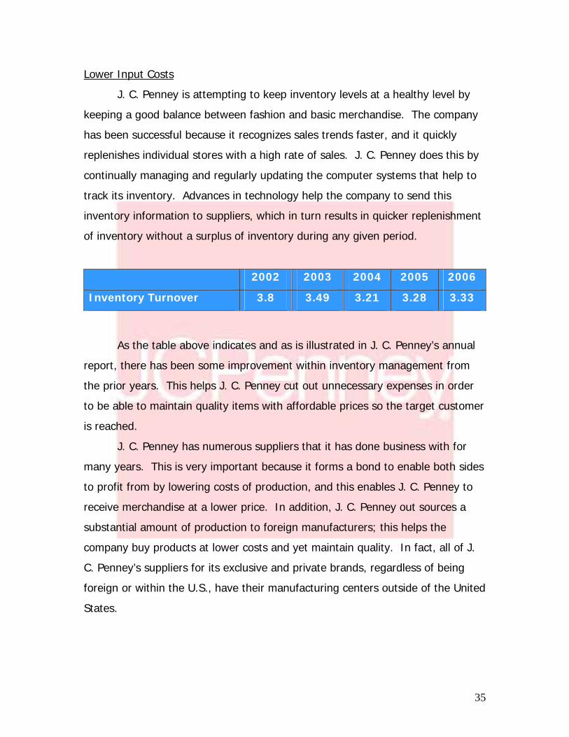
J. C. Penney is attempting to keep inventory levels at a healthy level by

keeping a good balance between fashion and basic merchandise. The company

has been successful because it recognizes sales trends faster, and it quickly

replenishes individual stores with a high rate of sales. J. C. Penney does this by

continually managing and regularly updating the computer systems that help to

track its inventory. Advances in technology help the company to send this

inventory information to suppliers, which in turn results in quicker replenishment

of inventory without a surplus of inventory during any given period.

2002 2003 2004 2005 2006

Inventory Turnover 3.8 3.49 3.21 3.28 3.33

As the table above indicates and as is illustrated in J. C. Penney’s annual

report, there has been some improvement within inventory management from

the prior years. This helps J. C. Penney cut out unnecessary expenses in order

to be able to maintain quality items with affordable prices so the target customer

is reached.

J. C. Penney has numerous suppliers that it has done business with for

many years. This is very important because it forms a bond to enable both sides

to profit from by lowering costs of production, and this enables J. C. Penney to

receive merchandise at a lower price. In addition, J. C. Penney out sources a

substantial amount of production to foreign manufacturers; this helps the

company buy products at lower costs and yet maintain quality. In fact, all of J.

C. Penney’s suppliers for its exclusive and private brands, regardless of being

foreign or within the U.S., have their manufacturing centers outside of the United

States.

36

Tight Cost Control System

J. C. Penney, during implementation of its turnaround plan, realized that

something had to be done about its cost control system in order to reach the

target customer. J. C. Penney had a decentralized system with branch managers

in charge of displays and available inventory. This has changed to a standard

floor design and product layout for consistency across many stores and reduces

costs in the long run. In addition, J.C. Penney now has thirteen key distribution

centers to lower the cost of distribution and increase accessibility. The centers

have the ability to reroute orders and deliveries.

Another way J. C. Penney has reduced costs has been by finalizing

installations of POS (Point of Sale) systems within all stores. This helps make

quicker transactions, and it also connects all stores via the internet to keep a

running count of all inventory at all times. This helps the stores in many ways.

For one, the inventory POS system reduces the amount of staff needed to make

the sale to customers due to a quicker transaction, which in turn drives down

costs of labor. Also, knowledge of amount of inventory helps J. C. Penney keep

a semi-accurate count all products on hand, disposing the idea of excess

inventory that creates waste. Finally, as mentioned earlier, J. C. Penney has

foreign suppliers as they outsource all private brand merchandise from both its

foreign and domestic suppliers, which also helps to reduce the cost of purchasing

supplies.

Operating Expenses over Sales

2002 2003 2004 2005 2006

Operating Expenses/

Sales .98 .97 .94 .92 .91

The table above shows how J. C. Penney has been successful in

marinating tight cost controls in the last five years. As one can see, the amount

of operating expenses per dollar made in sales has been reduced by seven cents

37

in the last five years. This trend will more than likely be reduced even more now

that the implementation of the POS systems has been established in all locations

this past year.

Gross Profit Margin

2002 2003 2004 2005 2006 JCP 0.3076 0.3722 0.3875 0.3927 0.3932 KSS 0.3442 0.3302 0.3516 0.3554 0.3637 DDS 0.3805 0.4583 0.5007 0.5305 0.5188 SSI 0.3029 0.2876 0.2891 0.2912 0.2925 SMRT 0.2474 0.2514 0.2664 0.2809 0.2773

Product Quality and Variety

J. C. Penney offers a wide variety of brands and product in its stores and

online. Many of these brands have been created as private brands through J. C.

Penney “as response to feedback from customers and research of direct

competitors” (J. C. Penney 2006 10-K). A recent example, according to the J. C.

Penney 2006 10-K, is the new private label lingerie brand, Ambrielle. “Ambrielle

was created to fill a void in the marketplace for a sensual lingerie brand targeted

to the modern customer at a smart price” (J.C. Penney 2006 10-K). This is just

one of the many examples of brand creation by the company to bring in a wider

range of customers that enjoy style at the right price. At J.C. Penney, the

consumer has the choice between varieties of quality goods.

Investment in Brand Image

Not only do private brands bring in loyal customers, contracts with

popular brand names also attract other consumers to places they may not

usually go. Fans of the popular cosmetic brand, Sephora, will visit J. C. Penney

just to purchase these products then “shop around” the store, creating more

revenues for the company. J. C. Penney is not only selling Sephora products but

is also talking with Polo Ralph Lauren’s Global Brand Concepts. This talk “has

recently launched a new lifestyle brand, American Living, created exclusively for

38

the J. C. Penney customer” (J. C. Penney 2006 10-K). Examples such as these

show how J. C. Penney strives to differentiate the merchandise in its stores,

creating a mix of product that ultimately stands out to the consumer as superior

than the rest. This seems to have ultimately paid off because as J. C. Penney

“continues to expand its stable of private brands; (they) now account for about

45 percent of sales” (Covert, Wall Street Journal).

Investment in Research and Development

According the 2006 10-K report, J. C. Penney “has taken several actions to

improve the customer shopping experience across all channels, including more

closely aligning stores and Direct promotions.” An example of how the company

has implemented its findings is seen by looking at the a.n.a. brand, which targets

working women. This clothing line implements a style that is classy enough to

wear during the week but not too formal for the weekend. The flexibility of this

line of clothing is what was demanded by the working women of today. J. C.

Penney has also responded to the recent demands of the retail industry focusing

on expansion within non-mall locations. J. C. Penney’s “250 stores it plans to

open in the next five years will be stand-alone entities, not connected to

shopping malls” ( O’Connell, Wall Street Journal).

Looking Ahead

J. C. Penney has repositioned itself within the department store industry

to identify with its target consumer, the middle-income family that would like to

affordable quality products. To reach this target consumer in more areas as well

as maintain a healthy growth rate, J. C. Penney is growing the number of stores

in operation. The current agenda for the company is to open 50 new stores per

year from 2007 to 2009. This will help the company continue to capitalize on the

present advantage of being one of the largest department retailers in the United

States with 1,033 departments across 49 states. J. C. Penney is also focusing on

the latest idea of opening more locations in places that are freestanding and

39

convenient for different consumers other than those who shop in malls on a

regular basis.

The continuous balancing act between keeping the correct mixture of cost

leadership while carrying above average merchandise is an issue that J. C.

Penney will have to always need to re-evaluate on a regular basis to sustain the

competitive advantage. The company seems to do well at this as they

implement new inventory tracking systems while creating and developing private

brands.

40

Accounting Analysis

Financial statements are prepared to provide shareholders and

other potential investors with a more informative view as to the value of a

company. They are designed to answer the fundamental questions of how the

business is currently performing and what its future prospects are. By answering

these questions, these financial statements offer the company’s investors with

information needed to make informed decisions, whether it be to invest in the

company or finance the firm’s future endeavors. The accounting analysis must

be done with a healthy level of skepticism due to the flexibility provided by the

Generally Accepted Accounting Practices (GAAP). Management has been given

this discretion in order to give a more informative and clearer understanding of

their company. This leads to estimates and assumptions involving judgment that

could lead to some errors. An accounting analysis is a tool used by financial

analysts to investigate the extent of these errors. It is used to determine the

accuracy of the statements provided by financial managers of a particular firm.

The accounting analysis process consists of six steps. First, the key

accounting policies must be identified. These policies are used to measure the

firm’s key success factors and its potential risks. “A critical accounting policy is a

policy for a company of an industry which is considered to have a notably high

subjective element, and that has a material impact on the financial statements”

(www.wikipedia.com). Next, an assessment of accounting flexibility allowed by

GAAP must be performed. Not every company has equal amounts of flexibility

when deciding upon which key accounting policies to utilize. Therefore, this

flexibility must be looked into and addressed. Once the accounting flexibility is

determined, an evaluation of the firm’s accounting strategy is conducted. This

evaluation determines how consistent the firm’s accounting policies are with its

competitors. It also looks into the financial managers’ incentive base, whether

the firm has recently changed or altered its policies, and if any business

41

transactions have been improperly structured to achieve certain accounting

objectives (Business Analysis & Valuation).

The fourth step of the accounting analysis process is to evaluate the

quality of disclosure. This evaluation determines the level of transparency that a

firm has within its financial statements. The higher the level of transparency, the

more accurate the financial statements tend to be. In addition, this transparency

allows investors to get a more informative view of the actual performance of the

firm. During this accounting quality analysis, potential “red flags” should be

identified. They typically are unexplained or unusual changes in numbers

reported in the statements. These are alerts that poor accounting quality has

been used. Once flexibility, disclosure, and “red flags” have been identified, the

analyst must undo any accounting distortions found within the firm’s financial

statements in order to provide accurate information to the investors.

Key Accounting Policies

A company’s key success factors should always be looked at when a firm

is deciding upon which key accounting policies to use. This is because these

success factors add value to the firm by giving it an advantage over its

competition. J. C. Penney’s key success factors, as mentioned within the five

forces model, are economies of scale, tight cost control, and investment in brand

image. Since there is generally not a lot of differentiation between the majority

of products sold within this particular industry, firms want to have every

advantage possible in order to set themselves apart from their competition.

Investing in a company’s brand image is another way to gain a competitive

advantage within the departmental retail industry. Brand image is about getting

your consumers to remember your name and products. However, the cost of

getting the word out can be rather high. Keeping costs low is the main way in

which a firm can gain an advantage over its competition. Flexibility within GAAP

can be used by firms to either clearly disclose their financial information or adjust

42

their numbers to be more appealing to investors than they would have

otherwise. The following are the accounting policies derived from J. C. Penney’s

key success factors.

Continuous Growth

The high competition of department and discount segment of retail stores

forces companies to be cost competitive. Taking advantage of economies of

scale, firms can reduce fixed cost by distributing it through a larger amount of

purchases. This helps maintain prices competitive without reducing the quality.

Having a healthy continuous sales growth helps to achieve this. J. C. Penney has

achieved a sixth consecutive year of comparable department store sales growth

averaging more than 3 percent increase per year (J.C. Penney 2006 10-K). The

table below illustrates the percentage growth for the last five years within the

company. Internet sales growth has had a large impact in the firm accounting

partially for the turnaround of the direct channels sales growth.

Sales Growth

2002 2003 2004 2005 2006

Comparable Department

Stores 2.6% .9% 4.9% 2.9% 3.7%

Internet 17.8% 50.8% 34% 28% 22%

Direct (Internet/Catalog) -22%** 3.3% 3.3% 3.6% 2.4%

* Percentages derived from the J. C. Penney 2006 10-K. **“In 2002, catalog was impacted by planned

lower page counts, lower circulation of catalog books, changes to payment policies and fewer

outlet stores” (2002 J. C. Penney 10-K).

Along with these sales growth percentages, J. C. Penney has started

accelerating the growth of new stores. It expects to grow 50 new stores from

2007 to 2009. Most of these new store locations opened will be operating or

capital leases. J. C. Penney owns 314 department stores as of April 2007. J. C.

43

Penney does state in its annual reports that “management intends to maintain

sufficient cash investment levels to ensure support for… contingency items, such

as the opportunistic purchase of selected real estate properties attributable to

consolidation within the retail industry” (J.C. Penney 2006 10-K). This shows

that J. C. Penney will invest in properties, if the opportunity were to arise, in

order to receive higher profits due to economies of scale.

J. C. Penney has both a line item in its income statement for pre-opening

expenses and real estate expenses with further explanation within its footnotes.

This shows a great amount of disclosure helping to maintain the level of

transparency within its annual reports. This is a key accounting policy because it

is very hard to have full disclosure during a high growth period whether it is

sales, size or both. This information could give insider information to

competitors that could jeopardize its strategic moves. J. C. Penney chooses to

maintain a high disclosure to keep the shareholders informed regardless of the

risk.

Post-Retirement Benefit Plans

Department and discount segment of retail stores, in order to continue

operating using its key success factors, must keep costs as low as possible. This

can lead to very aggressive accounting policies that will reduce the transparency

of their financial statements. A place that can be strongly influenced by this is

accounting for post retirement benefit plans. The judgment required to generate

the rate of discounting the pension benefit costs to present value can impact the

amount tremendously. J. C. Penney shows this by clarifying that “the sensitivity

of the pension expense to a plus or minus one-half of one percent of the

discount rate is a decrease or increase in expense of approximately $0.07 per

share” (J.C. Penney 2006 10-K). That is a large difference and could either

satisfy or dissatisfy shareholders.

44

Pension Discount Rates

2002 2003 2004 2005 2006

J.C. Penney 7.25% 7.1% 6.35% 5.85% 5.8%

Dillard’s 7.25% 6.75% 6.0% 5.5% 5.6%

Stage Stores Inc. 6.5% 6.5% 6.5% 6.0% 5.75%

Kohl’s N/A* N/A* N/A* N/A* N/A*

Stein Mart Inc. N/A* N/A* N/A* N/A* N/A*

* (discount rates not disclosed) **Percentages from the company’s 10-K’s

The table above shows the pension discount rates for the last five years

among top five department stores in the department and discount segment of

the retail industry. J. C. Penney, along with Dillard’s, has become less aggressive

with their generated discount rate showing figures that are more transparent;

these conservative discount rates help the present value cost amount to be more

reasonable compared to the actual expense. J. C. Penney lowered its discount

rate “…based on the yield to maturity of a representative portfolio of AA-rated

corporate bonds as of the October 31 measurement dates in 2005, 2004 and

2003, with average cash flow durations similar to the pension liability” (J. C.

Penney 2006 10-K).

These average discount rates show to outsiders of the industry that J. C.

Penney is not worried with large pension costs cutting into its net income.

Actually, J. C. Penny has seen a “… decrease in retirement-related benefit plan

expenses…” This “…was driven by the $60 million decrease in qualified pension

plan expense, which resulted from strong investment returns on the plan’s

assets” (J. C. Penney 2006 10-K). Overall, there has been an improvement of

disclosure of post-retirement benefit plans within the J. C. Penney annual

reports. This high level of disclosure along with the average discount rates used

show that J. C. Penney has been able to be confident in its accounting policies

along with the key success factors to be competitive within its industry by

maintaining costs low.

45

Operating and Capital Leases

Operating leases are widely used within the department and discount

retail store industry. They stay off the balance sheet helping to reduce liabilities,

or future obligations, the company may have. This distorts financials and can be

very hard to undo because most firms do not disclose lots of information

pertaining to these future obligations that generally can be for a large amount of

years. The industry uses them because costs seem to be lower than competitors

that may use capital leases. They appear to be cost efficient to shareholders. On

the other hand, capital leases are leases with characteristics of asset ownership.

They are amortized over either the economic life or asset life depending on the

amount of years for the lease.

J. C. Penney discloses a vast amount of information pertaining to capital

and operational leases. It discloses the future payments for the next five years,

the present value of these obligations, and even the discount rate used for both.

The obligation amount for both capital and operational leases are not substantial

amounts. This helps keep financials without significant distortions especially

since most information is disclosed within the footnotes about it, which shows

consistency with its level of disclosure. Overall, the level of disclosure and the

way they account of operational and capital leases is an important accounting

policy to J. C. Penney because of the potential changes it could have to the

presentation of expenses and costs. This is very important in this industry of

cost competition to maintain the shareholders as informed as possible especially

with its strategic growth that may increase its amount of operational and capital

leases.

Research and Development

With the new focus of J. C. Penney to reposition itself as not only

affordable prices but also quality to target customers, a lot research and

development has been spent for differentiation. Expenses have occurred in

things such as brand development, quality control, and advertising. In the past,

46

companies have erroneously capitalized these costs as an asset of the company

to maintain net income at an acceptable level. This is incorrect and is a policy

that must be looked on carefully.

J. C. Penney’s high disclosure annual reports show that these costs are

expensed as incurred, as they should be. Brand development and quality control

costs are expensed within cost of goods sold. This is because these are costs

“directly related to bringing merchandise to its final selling destination” (J. C.

Penney 2006 10-K). Advertising expenses are included within selling, general,

and administrative costs and are expensed when the advertising occurs for the

first time or as incurred.

This accounting policy is very important when part of the firm’s key

success factors is through differentiation. High costs may be incurred, and it is

very tempting to capitalize them as assets since they may seem to bring future

value to the firm. This is an error because the future benefits cannot be

calculated. Because of J. C. Penney’s high disclosure, an outsider is able to

verify that J. C. Penney expenses these costs as they do.

Conclusion

As more attention is shed upon firm’s that use creative accounting to

manipulate numbers in its favor, key accounting policies become factors that are

even more important to identify and look at carefully. The only way to ensure

the firm’s key accounting policies and receive a clear understanding is by having

transparent annual reports with high disclosure. These policies should support

the firm’s success factors in order for a company to be profitable. The key

accounting policies supported J. C. Penney’s key success factors of economies of

scale, lower input costs, tight cost control, and investment in brand image. This

can be verified by looking at the transparent financial statements and high

disclosure footnotes that ease the process of verifying.

47

Potential Accounting Flexibility

A firm provides financial statements in order to give investors the

information they need to make informed decisions regarding its investments

within the firm. This information should be relevant, reliable, and consistent.

Flexibility within GAAP allows financial statement preparers the opportunity to

present their company’s financial information in a more informative, qualitative

way. This flexibility, however, can cause some information in a company’s

financial reports to be distorted, making it seem more appealing to potential

investors. Some of the ways in which J. C. Penney has flexibility within GAAP are

discussed below.

Operating vs. Capital Leases

One of the main accounting policies that J. C. Penney has flexibility in is

whether to classify its leases as either operating or capital. With an operating

lease, the owner of the building or property only leases out the right to use it for

operating a business. When the lease term is up, the lessee can either return

the property or renew his or her lease for an extended amount of time. Since

ownership does not transfer from the lessor to the lessee, the rent expenses are

only reflected on the income statement (as operating expenses) and not on the

company’s balance sheet. When these expenses are not listed on the balance

sheet, the company’s assets and/or liabilities can be significantly understated.

This in turn causes the firm’s expenses to be understated, the net income to be

overstated, and the firm’s retained earnings to be overstated. When the

retained earnings of a company are overstated, it appears more profitable than it

truly is. When a firm appears to be highly profitable, shareholders are more

inclined to invest in the business.

Capital leases, on the other hand, do affect the firm’s balance sheet.

They are listed as both a liability (lease payments) and an asset (additions to

PPE). This is because the lessee assumes risks (e.g. taxes, payments) and also

48

acquires certain benefits associated with ownership (e.g. depreciation, deduction

of interest expenses). Since these expenses are recognized sooner than later

while using capital leases, most departmental retail firms opt to use operational

leases instead. However, since the obligation amounts of both of these types of

leases are relatively low for J. C. Penney, the company has a lot of flexibility

when choosing which type of lease to apply to its financial reports.

Pensions

Pensions, or post-retirement benefit packages, represent a significant

financial liability for a firm. Flexibility within GAAP allows from many companies

to overstate their earnings therefore making adjustments for pension expenses.

Companies determine how much they will have to spend in the future on

retirement packages based on their employee base. These assumptions include

things like the overall age and expected retirement dates of their existing

employees. When a final number is decided on, the rates are discounted back

using the time value of money so that they have a present value for these future

expenses. The lower the discount rate, the higher the company’s assets because

there is less money going into this type of expense. With increased assets, there

is typically a higher rate of return for the firm. Reporting a higher rate of return

on assets means a higher profit and therefore a greater percentage paid out as

dividends to the investors. Fortune Magazine states that “a reasonable rate of

return on pension assets is between 6 and 7 percent.” J. C. Penney has

maintained a limit around this reasonable rate. Therefore, they have flexibility

with regard to what discount rate they utilize and still be within a normal range.

Conclusion

Flexibility within the generally accepted accounting procedures allows

firms to report their financial information to their investors in more detail.

However, firms can utilize this flexibility to distort and manipulate their financial

statements in order to make their company appear more profitable than they

49

truly are. J. C. Penney, however, has a relatively high level of disclosure within

its financial reports. Therefore, they use the flexibility allowed to them while

maintaining a certain level of transparency for their investor information.

Actual Accounting Strategy

Financial statements produced by companies are given a certain level of

discretion when creating their financials in accord with GAAP. They have the

option to make their documentation appear aggressive, conservative, or a

mixture of both. In using this leeway to their advantage, firms can manipulate

their performance to give a good economic understanding or hide the actual

performance of the company. After reviewing J. C. Penney’s previous financial

statements, it appears they have chosen to show both aggressive and

conservative documentation.

Some form of retirement plans are available through all department retail

stores. J. C. Penney has a defined benefit pension plan that is offered to all

employees after 1 full year of service or 1,000 hours of work. With these plans

come many assumptions that require significant judgment. “The Company

utilizes third parties, including actuarial and investment advisory firms, to help

evaluate the appropriateness of the expected rate of return, the discount rate

and other pension plan assumptions annually” (J. C. Penney 10-K 2006). Using

an outside source to help find estimations gives JCP a fair assessment of what

rates to state within their financials. As mentioned previously, J.C. Penney’s

pension discount rate has decrease substantially over the past five years from

7.25 to 5.8 percent. Investopedia.com claims that a lower the discount rate

used on pension cost/expenses will cause the overall cost of these expenses to

increase (www.investopedia.com). From this point of view, you could state this

lowering of rates as a conservative action of these firms. As shown in the

previous graph, this has been an industry wide change over the past five years.

This had little change on the recording of pension expenses for J. C. Penney; in

50

2006, they made several changes to their recognition of defined benefit plans.

The changes should have a stronger showing on the 2007 financials, but no

substantial changes that would affect the company’s statements.

Most department store retailers have a large amount of operating leases

on their books, and J. C. Penney is no different. They have a substantial amount

of operating leases amounting to a present value of $944 million, while holding

only $8 million of capital leases on record. Firms choose to record these leases

as operating because, “the lessee does not assume the risk of ownership, the

lease expense is treated as an operating expense in the income statement and

the lease does not affect the balance sheet” (Capital Resources, www.cr-

ny.com). This is considered to be an aggressive accounting technique, but one

that most retailers disclose in their financials.

J. C. Penney offers many allowances through different programs in order

to maintain good relations with their suppliers. These practices include discounts

on advertising, markdown reimbursements, and for defective merchandise, all of

which require specific conditions for their allowance or repayment. Such as for

use when recording markdowns, when reimbursements are encountered with

merchandise that has been sold, the loss is directly related to the cost of goods

sold for the period encountered. In the case that allowances are encountered

with the vendor before the merchandise is sold, the record is documented with

association to the merchandise cost. This technique would be considered

somewhat conservative, and as well an industry standard practice.

Quality of Disclosure

The quality of communication between the company and those who study

the financial position or direction of the company in respect to annual reports is

crucial in determining the confidence of those outside the company looking in.

The following sections discuss the worth of the J. C. Penney’s annual reports in

both a qualitative and quantitative perspective.

51

Qualitative Analysis of Disclosure

The quality of disclosure relating to the footnotes and discussion should

be the best the company can offer to the public without giving competitive

secrets away. It is important for analyst to believe they are receiving the best

information they can so that these people have confidence in the company’s

direction and guidance. Having a confidence in a company form the

shareholders helps to shed positive light on future projects with eager skepticism

rather than suspicion. Assurance of these statements is achieved by how well

the company speaks about what is happening in the financial statements.

Pensions

J. C. Penney does a very good job in relaying information of current

happenings regarding new brands and product lines as well as financial

positioning and reasoning. One example of how the company strives to be as

transparent as is the manner in which J. C. Penney shares information on

pension plans. This particular subject is one of interest to the investing

community because this is an area that companies have the flexibility to distort

financial statements and mislead analysts’ beliefs of their financial positions.

J. C. Penney tries very hard to give all the information possible to create a clear

picture of where the numbers on the financials come from. Not only is there

discussion of pension plan benefits and contributions in the manager’s discussion

and analysis section the 2006 10-K, but the company also provides a very

detailed section in the appendices of how exactly the number materialize.

Within all eight pages of discussion and proven numbers, J. C. Penney

goes into detail on issues such as who is allowed to receive benefits, primary and

supplemental plans, expenses of such plans, how they are funded, and the

actual discount rates of all plans. Unlike some companies in the industry, J. C.

Penney discloses the discount rates of the plans, saving analysts the trouble of

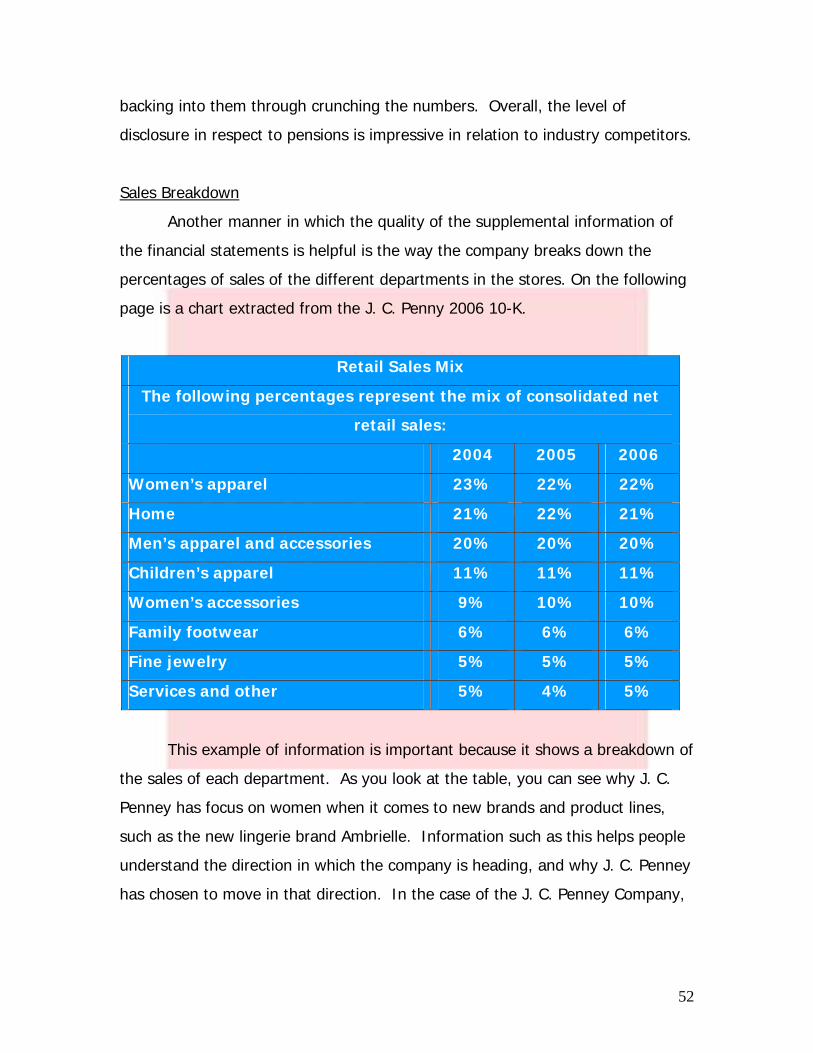
52

backing into them through crunching the numbers. Overall, the level of

disclosure in respect to pensions is impressive in relation to industry competitors.

Sales Breakdown

Another manner in which the quality of the supplemental information of

the financial statements is helpful is the way the company breaks down the

percentages of sales of the different departments in the stores. On the following

page is a chart extracted from the J. C. Penny 2006 10-K.

Retail Sales Mix

The following percentages represent the mix of consolidated net

retail sales:

2004 2005 2006

Women’s apparel 23% 22% 22%

Home 21% 22% 21%

Men’s apparel and accessories 20% 20% 20%

Children’s apparel 11% 11% 11%

Women’s accessories 9% 10% 10%

Family footwear 6% 6% 6%

Fine jewelry 5% 5% 5%

Services and other 5% 4% 5%

This example of information is important because it shows a breakdown of

the sales of each department. As you look at the table, you can see why J. C.

Penney has focus on women when it comes to new brands and product lines,

such as the new lingerie brand Ambrielle. Information such as this helps people

understand the direction in which the company is heading, and why J. C. Penney

has chosen to move in that direction. In the case of the J. C. Penney Company,

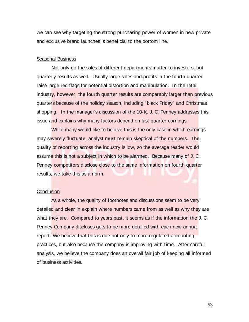
53

we can see why targeting the strong purchasing power of women in new private

and exclusive brand launches is beneficial to the bottom line.

Seasonal Business

Not only do the sales of different departments matter to investors, but

quarterly results as well. Usually large sales and profits in the fourth quarter

raise large red flags for potential distortion and manipulation. In the retail

industry, however, the fourth quarter results are comparably larger than previous

quarters because of the holiday season, including “black Friday” and Christmas

shopping. In the manager’s discussion of the 10-K, J. C. Penney addresses this

issue and explains why many factors depend on last quarter earnings.

While many would like to believe this is the only case in which earnings

may severely fluctuate, analyst must remain skeptical of the numbers. The

quality of reporting across the industry is low, so the average reader would

assume this is not a subject in which to be alarmed. Because many of J. C.

Penney competitors disclose close to the same information on fourth quarter

results, we take this as a norm.

Conclusion

As a whole, the quality of footnotes and discussions seem to be very

detailed and clear in explain where numbers came from as well as why they are

what they are. Compared to years past, it seems as if the information the J. C.

Penney Company discloses gets to be more detailed with each new annual

report. We believe that this is due not only to more regulated accounting

practices, but also because the company is improving with time. After careful

analysis, we believe the company does an overall fair job of keeping all informed

of business activities.

54

Quantitative Analysis of Disclosure

Generally Accepted Accounting Principles (GAAP) provide managers with

flexibility. This flexibility is valuable because it allows managers to better portray

the performance of their firms through the financial statements. In addition, this

flexibility helps managers to create a clearer picture of the financial health of the

company. However, since there is incentive for managers to distort a company’s

actual performance, it is important that analysts, regulators, and investors, alike,

carefully scrutinize the numbers contained in those statements. Any significant

change in the numbers represented in the financial statements should be

thoroughly investigated.

Two categories of diagnostics utilized here to help better evaluate the

revenues and expenses of a firm are sales manipulation and expense

manipulation diagnostics. Comparing net sales to cash from sales, accounts

receivables, inventory, unearned revenues, and warranty liabilities over an

extended period, in this case five years, can aid analysts in pinpointing

accounting irregularities used to puff up performance. Like wise, comparing

expenses, cash flows, accruals, and asset turnover from one year to the next can

help identify inappropriate manipulation of reported information. Unexplained

increases or decreases in any of these ratios may be a “red flag” that could

potentially expose a serious financial health problem, improper accounting

practices, or even fraud.

Sales Manipulation Diagnostics

Examining the sales performance of a company across several years

allows analysts to identify any potential discrepancies in reporting from one year

to the next. Examining the sales performance of a company against that of its

competitors in the industry allows analysts to check if identified anomalies are

industry wide or company specific. The following section contains sales

55

manipulation diagnostics for J. C. Penny, Kohl’s, Dillard’s, Stage Stores, Inc., and

Stein Mart, Inc.

Net Sales/Cash From Sales

Net Sales/Cash From Sales

0.4

0.6

0.8

1

1.2

1.4

1.6

2002 2003 2004 2005 2006

Year

JCPKSSDDSSSISMRT

The ratio of net sales to cash from sales compares sales minus returns to

the amount of cash actually received from those transactions each year. A 1:1

ratio is ideal; however, in most cases, impractical. A large percentage of

consumers use credit cards to make purchases. If a customer uses a major

credit card like Master Card, Visa, or Discover, revenues can be booked as cash

almost immediately, since the liability of default falls on the creditor’s shoulders

and not the retailer’s. However, if using a private label credit card, the revenue

must be booked as a receivable and payment must be collected before it can be

recognized as cash.

Most companies in the department and discount segment of the retail

industry do not have private label credit cards due to the high risk of default.

Typically, firms will pay a small fee to have a major credit card company accept

that risk for them. Among the firms evaluated here, J. C. Penney is the only

56

company still using a private label credit card. In 2004, J. C. Penney

experienced an increase in the use of its private label credit card, which explains

the sudden deviation from the industry norm. Dillard’s had a private label credit

up until 2004, when it sold its credit card company to GE Finance Company

(Dillard’s 2007 10K), explaining the rapid increase in its ratio of net sales to cash

from sales from 0.8:1 to 1:1. Overall, this specific ratio is supported by the J. C.

Penney financial statements.

57

Net Sales/Net Accounts Receivable

Net Sales/Net Accounts Receivable

-100

0

100

200

300

400

500

600

700

800

2002 2003 2004 2005 2006

Year

JCPKSSDDSSSISMRT

When examining net sales in relation to accounts receivable, you can see

that the industry, with the exception of Dillard’s and Stein Mart, maintains a fairly

low ratio. J. C. Penney did not show in drastic rises in this ratio, indicated that

over the last five years, sales have been supported by account receivables on a

consistent basis. This shows fairly stable. Other players in the industry have

almost zero accounts receivable because they have no company credit card

operations whereas J. C. Penney does. In 2004, J. C. Penney’s net

sales/accounts receivable ratio dipped due to the sale of Eckerd Pharmacy, then

rose due to higher sales in 2005.

Other companies in the department and discount segment of the retail

industry seem to maintain relatively acceptable amounts of accounts receivable,

with the exception of Dillard’s and Kohl’s, where accounts receivable accounted

for up to 17 and 13 percent of their net sales, respectively. In an effort to

correct this problem, Dillard’s sold its private label credit card company to GE

Finance Company in 2004, and Kohl’s factored its accounts receivable and sold

them to JP Morgan Chase in 2005 (Kohl’s 2007 10K). This reduced Kohl’s

58

accounts receivable to zero resulting in a ratio that no longer applies to the

company.

Net Sales/Inventory

Net Sales/Inventory

0

1

2

3

4

5

6

7

2002 2003 2004 2005 2006

Year

JCPKSSDDSSSISMRT

Over the last five years, all five companies looked at in this industry have

maintained a relatively steady inventory turnover. Even in the event of the sales

of businesses in the last three years, J. C. Penney had preserved a steady ratio.

In essence, this ratio evaluates how well a firm uses its inventory to generate

revenue. Because it has not spiked unexpectedly, there are no indicators that

sales have been overstated in respect to inventory.

59

Net Sales/Unearned Revenue

Net Sales/Unearned Revenue

0

200

400

600

800

1000

1200

2002 2003 2004 2005 2006

Year

JCPKSSDDSSSISMRT

When evaluating the ratio of net sales to unearned revenue, analysts look

for unexplained changes in the level of unearned revenue. For instance, if the

ratio of net sales to unearned revenue increases dramatically, the firm may be

recognizing revenue before it is actually earned in an effort to improve earnings.

Firms sometimes do this in order to improve sales numbers, when actual sales

come in below estimates. This sort of manipulation is cause for concern and is a

potential “red flag” indicating fraudulent behavior.

Looking at this graph, we see a great deal of variation in the ratio

between firms. Some of this activity is explainable. For instance, Dillard’s and

Kohl’s sudden rise in unearned revenue was most likely caused by a change in

disclosure. In previous years, Dillard’s and Kohl’s did a poor job of separating its

unearned revenues from its other liabilities. In 2004 and 2006, respectively,

Dillard’s and Kohl’s disaggregated their liabilities to reveal unearned revenue

liabilities from gift cards, which is a common practice among companies in the

retail industry.

60

Net Sales/Warranty Liabilities

None of the companies examined in this report offer warranties or

extended warranties on any of their products or services. All warranties

associated with products and services sold through these retailers are

manufacture warranties. The firms in this report have no warranty liabilities

compare against net sales; therefore, the ratio of net sales to warranty liabilities

does not apply to this segment of the retail industry.

61

Below is a chart of sales manipulation diagnostics used to create previous graphs

of J.C. Penney and industry competitors.

Sales Manipulation Diagnostics JCP

2002

2003

2004

2005

2006 Net Sales/Cash From Sales 0.9944 1.0249 0.8153 0.9185 0.9996 Net Sales/Net Account Receivables 45.882 76.334 45.603 69.559 75.676 Net Sales/Inventory 6.5413 5.6356 5.8138 5.8507 5.8538 Net Sales/Unearned Revenues 186.97 92.155 89.004 85.757 86.160 Net Sales/Warranty Liabilities n/a n/a n/a n/a n/a KKS

Net Sales/Cash From Sales 1.0270 0.9935 1.0185 1.0135 1.0263 Net Sales/Net Account Receivables 9.2048 8.9397 8.4199 8.1124 n/a Net Sales/Inventory 5.6055 6.3983 6.0096 5.9896 6.0060 Net Sales/Unearned Revenues n/a n/a n/a n/a 1036.2 Net Sales/Warranty Liabilities n/a n/a n/a n/a n/a DDS

Net Sales/Cash From Sales 1.0344 0.9810 0.8643 1.0003 0.9997 Net Sales/Net Account Receivables 5.9121 6.3776 780.08 603.70 726.68 Net Sales/Inventory 4.9620 4.6551 4.3441 4.1938 4.3089 Net Sales/Unearned Revenues n/a n/a n/a 100.40 101.95 Net Sales/Warranty Liabilities n/a n/a n/a n/a n/a SSI

Net Sales/Cash From Sales 0.9994 1.0254 0.9725 1.0000 1.0000 Net Sales/Net Account Receivables 79.430 27.688 n/a n/a n/a Net Sales/Inventory 4.8663 3.7437 4.4172 4.7383 4.6585 Net Sales/Unearned Revenues 182.40 110.47 12.076 107.52 336.99 Net Sales/Warranty Liabilities n/a n/a n/a n/a n/a SMRT

Net Sales/Cash From Sales 1.0108 1.0068 1.0072 1.0066 1.0068 Net Sales/Net Account Receivables 286.36 320.66 249.42 133.22 147.70 Net Sales/Inventory 3.4339 3.4487 3.0755 2.8501 3.1254 Net Sales/Unearned Revenues n/a n/a n/a n/a n/a Net Sales/Warranty Liabilities n/a n/a n/a n/a n/a

62

Expense Manipulation Diagnostics

Examining the sales performance of a company across several years

allows analysts to identify any potential discrepancy in reporting from one year

to the next. Examining the sales performance of a company against that of its

competitors in the industry allows analysts to check if identified anomalies are

industry wide or company specific. The following section contains expense

manipulation diagnostics for J. C. Penny, Kohl’s, Dillard’s, Stage Stores, Inc., and

Stein Mart, Inc.

Asset Turnover

Asset Turnover

0

0.5

1

1.5

2

2.5

3

3.5

4

2002 2003 2004 2005 2006

Year

JCPKSSDDSSSISMRT

Asset turnover for J. C. Penney has also maintained steady of the last five

years. An increase in this ratio would show a red flag indicating assets were

overstated. As you can see, the ratio slightly increases overtime. This is not due

to a great change in assets but an increase in sales 2004 and on after the sale of

unprofitable businesses.

63

As for the industry, all the companies examined in this report have about

the same asset turnover ratio with one obvious exception, Stein Mart, Inc. Stein

Mart, Inc. achieves a significantly higher asset turnover ratio because it uses a

variation of the just-in-time inventory method in order to keep on hand inventory

as low as possible.

Cash Flows From Operating Activities/Operating Income

CFFO/OI

0

0.5

1

1.5

2

2.5

3

3.5

4

2002 2003 2004 2005 2006

Year

JCPKSSDDSSSISMRT

The cash flows from operating activities to operating income ratio links

the amount of cash generated by operating activities to the amount of operating

income reported on the income statement. A lower ratio is preferred because it

shows that more cash is generated by operating activities rather than investing

or financing activities. Over the past few years, there has been a downward

trend in this ratio in the retail industry. In other words, firms in the department

and discount segment of the retail industry are creating more income through

operating activities.

64

Cash Flows From Operating Activities/Net Operating Assets

CFFO/NOA

0

0.2

0.4

0.6

0.8

1

1.2

1.4

1.6

1.8

2002 2003 2004 2005 2006

Year

JCPKSSDDSSSISMRT

The ratio of cash flows from operating activities to net operating assets

links the cash flows from operating activities to a firm’s fixed assets, property,

plant, and equipment. The higher the ratio the more income generated by those

fixed assets. Most companies in the department and discount segment of the

retail industry have low ratios of CFFO/NOA due the practice of expensing large

fixed assets like property and buildings instead of capitalizing them. Although,

this is a questionable accounting practice, it is perfectly legal and widely used by

firms in this industry.

65

Pension Expense/SG&A

Pension Expense/SG&A

-0.4

-0.2

0

0.2

0.4

0.6

0.8

1

2002 2003 2004 2005 2006

Year

JCPKSSDDSSSISMRT

The pension expense to selling, general, and administrative expense ratio

shows the relationship between pension expense and operating expenses.

Effectively, this ratio is used to determine if a company is spending too much

money on its retirees. A lower ratio is preferred because it shows that pension

expense makes up an insignificant amount of the companies overall expenses.

Pension and retirement expenses expend resources that could be put to better

use within the company. In other words, a firm should not be spending a great

deal of money on people who are no longer employed by the company. Overall,

all firms in the department and discount segment of the retail industry maintain a

low pension expense to selling, general, and administrative expense ratio.

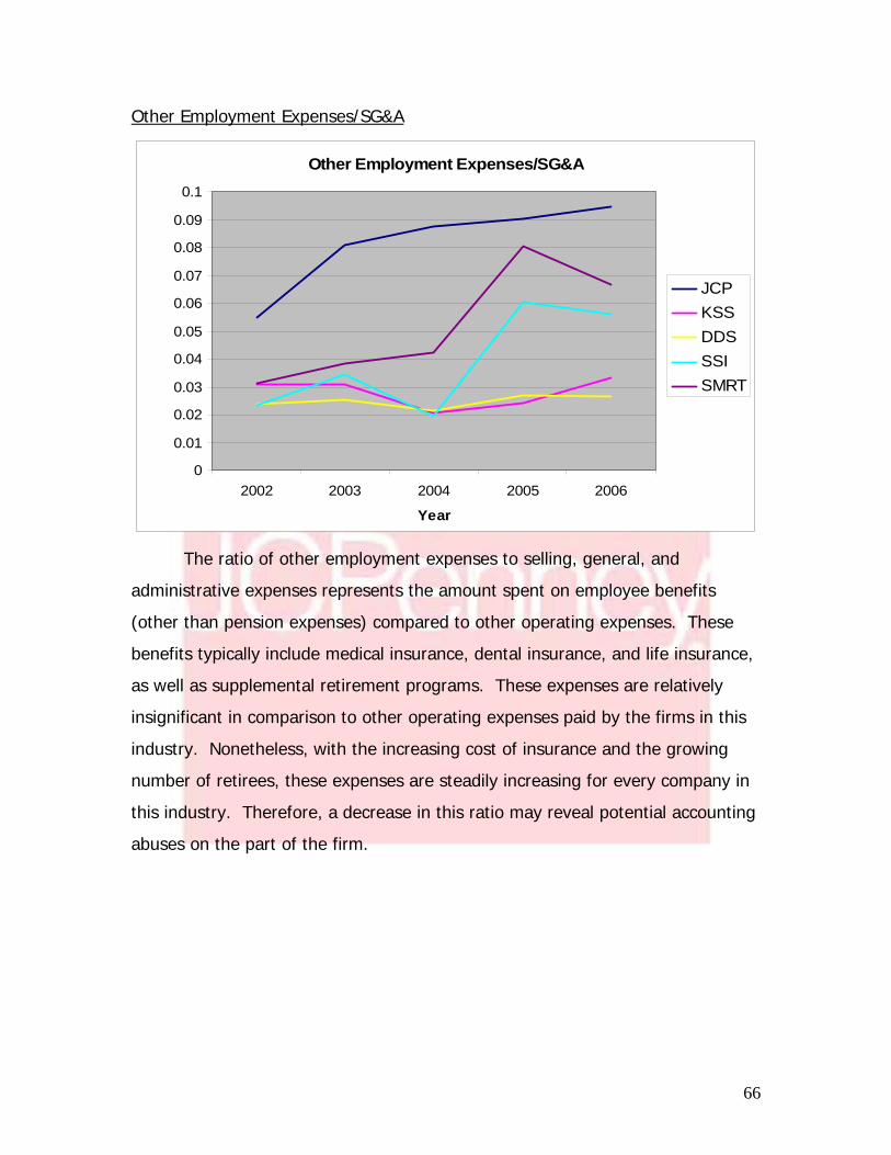
66

Other Employment Expenses/SG&A

Other Employment Expenses/SG&A

0

0.01

0.02

0.03

0.04

0.05

0.06

0.07

0.08

0.09

0.1

2002 2003 2004 2005 2006

Year

JCPKSSDDSSSISMRT

The ratio of other employment expenses to selling, general, and

administrative expenses represents the amount spent on employee benefits

(other than pension expenses) compared to other operating expenses. These

benefits typically include medical insurance, dental insurance, and life insurance,

as well as supplemental retirement programs. These expenses are relatively

insignificant in comparison to other operating expenses paid by the firms in this

industry. Nonetheless, with the increasing cost of insurance and the growing

number of retirees, these expenses are steadily increasing for every company in

this industry. Therefore, a decrease in this ratio may reveal potential accounting

abuses on the part of the firm.

67

Below is a chart of all expense manipulation diagnostics used to create the above

graphs comparing J. C. Penney to industry competitors.

Expense Manipulation Diagnostics JCP

2002

2003

2004

2005

2006 CFFO/OI 1.3106 1.0278 0.8589 0.8478 0.6529 CFFO/NOA 0.2711 0.2310 0.3097 0.3567 0.3015 Asset Turnover 1.8104 0.9719 1.3041 1.5071 1.5705 Total Accruals/Change in Sales 90.431 -1.1657 27.111 48.862 16.620 Pension Expense/SG&A 0.0027 0.0222 0.0140 0.0118 0.0016 Other Employment Expenses/SG&A 0.0549 0.0809 0.0876 0.0900 0.0945 KKS

CFFO/OI 0.6140 0.7372 0.7662 0.6225 1.7078 CFFO/NOA 0.1995 0.1840 0.1905 0.1523 0.4423 Asset Turnover 1.4441 1.5349 1.4663 1.4642 1.7192 Total Accruals/Change in Sales 0.3160 0.4357 0.3786 0.5335 -0.517 Pension Expense/SG&A n/a n/a n/a n/a n/a Other Employment Expenses/SG&A 0.0309 0.0309 0.0206 0.0244 0.0330 DDS

CFFO/OI 0.7998 1.7945 1.6152 1.2179 1.1092 CFFO/NOA 0.1059 0.1351 0.1741 0.1168 0.1141 Asset Turnover 1.1850 1.1852 1.3227 1.3703 1.4119 Total Accruals/Change in Sales -30.970 -22.966 -99.123 227.42 95.900 Pension Expense/SG&A 0.6183 0.5679 0.0045 0.0061 0.0050 Other Employment Expenses/SG&A 0.0236 0.0255 0.0212 0.0269 0.0265 SSI

CFFO/OI 0.3963 1.1171 0.3682 0.2708 0.1216 CFFO/NOA 0.7738 1.6358 0.6239 0.4342 0.1978 Asset Turnover 1.6434 1.4747 1.8105 1.8370 1.8790 Total Accruals/Change in Sales -0.1053 -2.6626 -0.2982 -0.4999 0.0006 Pension Expense/SG&A 0.0012 0.0016 0.0002 0.0002 0.0006 Other Employment Expenses/SG&A 0.0232 0.0345 0.0192 0.0603 0.0561 SMRT

CFFO/OI 0.9650 3.7645 1.8966 0.9717 0.5234 CFFO/NOA 0.4020 0.3882 1.6324 0.8766 0.2677 Asset Turnover 3.4339 3.4487 3.0755 2.8501 3.1254 Total Accruals/Change in Sales -0.1585 0.5201 -0.7489 -1.1577 0.3484 Pension Expense/SG&A 0.0049 0.0030 0.0028 0.0023 0.0036 Other Employment Expenses/SG&A 0.0313 0.0384 0.0420 0.0804 0.0664

68

Conclusion

Some firms within the department and discount segment of the retail

industry demonstrate some questionable accounting practices when compared to

their peers within the industry. However, such inconsistencies may be explained

by changes in accounting policies or unusually good (bad) sales activity.

Nonetheless, any inconsistency needs to be thoroughly investigated for

accounting abuse.

Of the firms evaluated by these sales and expense manipulation

diagnostics, J. C. Penney appears to be the most consistent in its accounting and

reporting practices. Although nothing unusual seems to be jumping off the

page, assuming J. C. Penney’s financial statements are complete and correct is

foolish. Analysts, regulators, and investors, alike, must have a healthy amount

of skepticism when using the financial statements of this firm, or any firm, to

make financial decisions.

Potential “Red Flags”

Accounting distortions can be found by examining the financial statements

and the information held there within using ratio analysis over a period of

comparative years. In the case of this accounting analysis, we have looked over

five years of data. The discrepancies found during this analysis are viewed as

red flags. These red flags could be accounting errors; however, they may be an

indication of accounting manipulation and abuse.

Potential red flags, in regards to the J.C. Penney Company, are limited.

Even with careful analysis, we were unable to find any significant discrepancies

in reporting. In fact, the annual 10-K reports filed with the SEC have improved,

making reporting and disclosures more transparent. Of all the firms we have

researched, which include the following: Stage Stores, Stein Mart, Kohl’s, and

Dillard, the J. C. Penney Company has the highest level of disclosure and the

most revealing financial statements. For example, J. C. Penney’s discloses

69

discount rates in respect to pensions. Not only does the company show these

rates, but they also go into detail on pension contributions and benefits in the

manager’s discussion and analysis section, as well as lengthy explanations in the

appendices.

Another example of the company’s high level of disclosure is the operating

and capital leases. J.C. Penney does an excellent job of disclosing the remaining

obligations of both types of leases. They are straightforward with the discount

rates of these leases, which takes the guesswork out of estimating. The

following shows the interest rates found within the most recent J. C. Penney 10-

K annual report.

Capital Leases 6.0 %

Operating Leases 7.9 %

Because this information is disclosed, backing into an interest rate for

future forecasts of the J. C. Penny is not required. The company also provides

the present value of all future lease payments for the next 20 years, according to

the 2006 10-K. Not only does this show that the company has no significant

distortions, it also shows the breadth and depth of the financial statements.

While analyzing the sales and expense ratios, one can agree that the J. C.

Penney Company is the most consistent in its accounting and reporting practices.

There were no relevant of significant errors in the ratio analysis to lead us to

believe there were any problems. It should be noted, however, analysts must

maintain a slight amount of skepticism when valuing the firm using company

financial statements.

Coming Undone (Undo Accounting Distortions)

After careful consideration and extensive research, we as a group have

70

concluded that there are no accounting distortions that need to be “undone.”

Once again, J.C. Penney is a very transparent business when compared to all of

the retail competitors in this specific industry. Re-estimation of lease

agreements was not necessary because all needed information was provided

within the footnotes and discussions relating to the financial statements. When

we compare the interest payments of all capital leases to the sum of all

operating lease payments, you can see the insignificance of operating leases.

Total 2007 2008 2009 2010 2011 After

5 yrs

Interest pmts on

LTD and capital

Leases

$5822 $253 $222 $218 $198 $178 $4753

Operating

Leases $1948 $213 $197 $170 $137 $112 $1119

Above, the chart shows exactly this, that the operating leases that are on the

financials are peanuts compared to the sales of J.C. Penney.

71

Financial Analysis, Forecast Financials, and

Cost of Capital Estimation

Financial Analysis

In an effort to accurately evaluate the overall financial health and

profitability of a firm, analysts have developed a series of ratios to breakdown a

firm’s financial statements into numbers that can be easily compared to those of

its competitors within its industry. The ratios most commonly used when

evaluating a company’s overall financial health and profitability are divided into

three categories: liquidity, profitability, and capital structure. By comparing the

ratios of companies within the same industry, analysts can draw conclusions

about the performance of a single firm in relation to its competitors. Simply put,

this section of the report will help determine how well J. C. Penney stacks up to

the competition.

Liquidity Analysis

Liquidity ratios are used to provide information about a firm’s ability to

meet its short-term financial obligations (www.netmba.com). Liquidity ratios

help lenders evaluate the credit risk associated with prospective borrowers.

Lenders generally prefer higher liquidity ratios because it demonstrates that a

firm has adequate resources to pay off its short-term financial obligations should

the need arise. Common liquidity ratios include the current ratio, quick ratio,

inventory turnover, receivables turnover, and working capital turnover. The

following section exams these ratios.

72

Current Ratio

Current Ratio

0.0

0.5

1.0

1.5

2.0

2.5

3.0

3.5

4.0

2002 2003 2004 2005 2006

Year

JCPKSSDDSSSISMRT

The current ratio is the relationship between a company’s current assets

(cash, cash equivalents, short-term investments, receivables, and inventory) and

the current or short-term liabilities (short-term debt and payables). The main

function of this ratio is to determine a company’s ability to pay back its short-

term liabilities in a hurry, should the need arise. The higher the ratio the more

likely a company will be able to pay off its obligations. For instance, a company

with a ratio of 1:1 has $1 of current assets for every $1 of short-term liabilities,

which means should there be able to pay off short-term liabilities immediately;

however, this just covers the basic need. A better turnover would be involve

more assets or less liabilities.

J. C. Penney typically maintains a current ratio of 2:1, which means that J.

C. Penney is unlikely to default on any of its short-term liabilities. Furthermore,

as you can see from the graph, some retailers have held current ratios as high as

3.5:1, but most companies within this segment have converged on 2:1. This

means that companies in this segment of the retail industry are capable of

73

paying off their short-term obligations with a fair degree of certainty. Overall, J.

C. Penney is inline with the industry standard.

Quick Ratio

Quick Asset Ratio

0.0

0.2

0.4

0.6

0.8

1.0

1.2

1.4

1.6

1.8

2002 2003 2004 2005 2006

Year

JCPKSSDDSSSISMRT

The quick ratio, otherwise known as the acid-test ratio, is the relationship

between a company’s current assets minus inventory (cash, cash equivalents,

short-term investments, and receivables) and its current liabilities. The quick

ratio is far more conservative than the current ratio because it excludes

inventory. This is because inventory can be difficult for a company to convert

into cash. Therefore, the quick ratio provides a clearer picture of a company’s

financial strength in the event it must pay off its short-term liabilities than the

fore mentioned current ratio.

J. C. Penney seems to keep a quick ratio of 0.8:1, meaning the company

only has $0.80 of liquid assets per $1 of short-term liabilities. Should J. C.

Penney have to pay off its short-term liabilities immediately, it may come across

a serious hurdle of liquidity. Although this is not the ideal situation for any

company and may be reason for concern, it is common in the retail industry,

74

where the largest portion of a company’s current assets is inventory. Although

the overall industry is converging, J. C. Penney still maintains one of the highest

quick ratios.

Receivables Turnover

Receivables Turnover

0

100

200

300

400

500

600

700

800

900

2002 2003 2004 2005 2006

Year

JCPKSSDDSSSISMRT

The receivables turnover ratio is the relationship between a company’s net

sales and its accounts receivable. The receivables turnover ratio is used to

evaluate how efficiently a firm uses its assets. A high ratio is preferred because

it suggests that a company operates primarily on a cash basis or that it efficiently

collects on its accounts receivable. For instance, if a company has a receivables

turnover ratio of 50:1, then the company generates $50 of revenue for every $1

of credit it extends.

Historically, J. C. Penney has maintained a receivables turnover ratio of

between 45 and 75; however, over the past four years this ratio has risen

steadily because of the company’s continuous earnings growth and the steady

retirement of its accounts receivable. This ratio is unusually high for J. C.

Penney, Stein Mart, and Dillard’s and not applicable to Kohl’s and Stage Stores

75

because many firms in this segment of the retail industry no longer finance their

private label credit cards. Today, companies like GE Finance Corporation provide

retailers with consumer finance services for a fee, which enable retailers to book

sales immediately.

Days Sales Outstanding

Days Supply of Receivables

0

10

20

30

40

50

60

70

2002 2003 2004 2005 2006

Year

JCPKSSDDSSSISMRT

Days sales outstanding is a measure of how long it takes for a company to

collect on its accounts receivables. This is also the second half of the cash-to-

cash cycle. The first half, days supply of inventory, is discussed later. In most

industries, this process varies from 30 days to 90 days, but in the department

and discount segment of the retail industry this number is typically low. For

instance, J. C. Penney’s days sales outstanding over the past five years has

averaged around six days. This is possible because J. C. Penney, like most

retailers in this industry, does not finance its own private label credit card.

Instead, J. C. Penney pays a fee to a company, like GE Finance Corporation, to

handle consumer credit cards. In essence, the private label credit card acts like

76

a MasterCard or VISA, allowing J. C. Penney to recognize revenues immediately

and keeps its accounts receivable minimized.

Inventory Turnover

Inventory Turnover

0

1

2

3

4

5

6

7

8

9

2002 2003 2004 2005 2006

Year

JCPKSSDDSSSISMRT

Inventory turnover is the ratio between cost of goods sold and its

inventory. Inventory turnover measures how many times a company sells and

replaces its inventory throughout the year. A low ratio suggests poor sales and

excess inventory. A high ratio implies strong sales or possibly insufficient

inventory levels. Because inventory ties up money that could be used for other

investment, it is important for a firm to maintain a steady turnover of its

inventory.

J. C. Penney has averaged a ratio of 3.5:1 over the past five years. In

other words, the company turns its inventory almost four times a year, or

approximately once every 3 ½ months. This means that cash is tied up in

inventory for almost 3 ½ months. Although this seems like a long time, it is very

common in the department and discount store segment of the retail industry due

to the seasonality of the product lines sold in these stores. In other words, J. C.

77

Penney’s inventory turnover is in line with the industry standard. Where as Stein

Mart outperforms the industry because it uses a variation of the just-in-time

inventory method to keep inventory low.

Days Supply of Inventory

Days Supply of Inventory

0

20

40

60

80

100

120

140

160

2002 2003 2004 2005 2006

Year

JCPKSSDDSSSISMRT

Days supply of inventory is a measure of how long inventory sits idle.

Days supply of inventory is the first half of the cash-to-cash cycle. In the case of

most firms in the department and discount segment of the retail industry,

inventory turns over approximately once every 90 to 120 days (once every 3 to 4

months). For instance, J. C. Penney turns its inventory every 103 days (3 ½

months). When you combine days supply of inventory with days sales

outstanding, you get the cash-to-cash cycle. In the case of J. C. Penney, the

cash-to-cash cycle takes approximately 109 days. This is quite common among

these firms due to the nature of the retail industry. The retail industry is prone

to affects of seasonality. Stores like J. C. Penney typically liquidate and replenish

their inventory with every season.

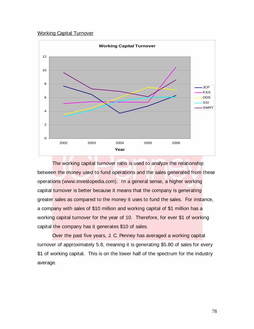
78

Working Capital Turnover

Working Capital Turnover

0

2

4

6

8

10

12

2002 2003 2004 2005 2006

Year

JCPKSSDDSSSISMRT

The working capital turnover ratio is used to analyze the relationship

between the money used to fund operations and the sales generated from these

operations (www.investopedia.com). In a general sense, a higher working

capital turnover is better because it means that the company is generating

greater sales as compared to the money it uses to fund the sales. For instance,

a company with sales of $10 million and working capital of $1 million has a

working capital turnover for the year of 10. Therefore, for ever $1 of working

capital the company has it generates $10 of sales.

Over the past five years, J. C. Penney has averaged a working capital

turnover of approximately 5.8, meaning it is generating $5.80 of sales for every

$1 of working capital. This is on the lower half of the spectrum for the industry

average.

79

Conclusion

Analysis through liquidity ratios shows that J. C. Penney is a liquid firm.

J. C. Penney’s current ratio, inventory turnover, receivables turnover, and

working capital turnover are all in line with the department and discount

segment of the retail industry. J. C. Penney slightly outperforms its peers in the

quick ratio, meaning it is potentially the most liquid firm evaluated in this report.

Profitability Analysis

The main objective of profitability analysis is to determine how efficiently

a firm can turn a profit. Profitability analysis is comprised of six ratios: gross

profit margin, operating expense ratio, net profit margin, asset turnover, return

on assets, and return on equity. The first three ratios measure a firm’s operating

efficiency, and the next three ratios measure asset productivity, return on assets,

and return on equity.

Gross Profit Margin

Gross Profit Margin

0.0

0.1

0.2

0.3

0.4

0.5

0.6

2002 2003 2004 2005 2006

Year

JCPKSSDDSSSISMRT

80

Gross profit margin is a ratio between a company’s revenues minus its

cost of goods sold compared to its revenues. The gross profit margin ratio

provides a quantitative analysis of the company’s ability to pay operating and

other expenses and build future savings. A high ratio is preferred because it

means the company has more money left after adjusting for costs of good sold

to pay bills and reinvest in the company for the purpose of growth.

J. C. Penney has maintained a gross profit margin of approximately 0.39

over the past four years, which is inline with the industry average. Prior to 2004,

J. C. Penney suffered lower gross profit margins due to the lagging performance

of the company’s subsidiary Eckerd Pharmacy, which the company sold to the

Jean Coutu Group (PJC) Inc. (Coutu) and CVS Corporation and CVS Pharmacy,

Inc. (together, CVS) in 2004. In comparison to the overall industry, J. C.

Penney’s performance is lined up with its competitors.

Operating Profit Margin

Operating Profit Margin

0.00

0.02

0.04

0.06

0.08

0.10

0.12

0.14

2002 2003 2004 2005 2006

Year

JCPKSSDDSSSISMRT

Operating profit margin compares the relationship between a firm’s

operating income and its sales. A higher operating profit margin indicates

81

operating efficiency because the firm is able to minimize its operating expenses.

A lower operating profit margin is an indicator of poor operating efficiency from

either declining sales or increasing operating expenses. Over the past five years,

J. C. Penney’s operating profit margin has been steadily increasing as other

firms’ operating profit margins are leveling out. This is inline with J. C. Penney’s

plan to increase operating efficiency and increase profitability.

Net Profit Margin

Net Profit Margin

-0.06

-0.04

-0.02

0.00

0.02

0.04

0.06

0.08

2002 2003 2004 2005 2006

Year

JCPKSSDDSSSISMRT

Net profit margin is a profitability ratio calculated by dividing net income

by sales. “Net profit margin measures how much out of each dollar of sales a

company actually keeps as earnings” (www.investopedia.com). A company’s net

profit margin does not say much about a firm’s performance, but when it is

compared to other companies within an industry, it proves to be very useful. A

higher net profit margin indicates that a company has better cost controls

compared to its competitors and is therefore more profitable.

J. C. Penney’s net profit margin has been steadily increasing over the past

five years, with the exception of 2003 when the company posted a loss of $1.3

82

billion from the discontinued operations of Eckerd Pharmacy. Overall, J. C.

Penney’s performance is beating the industry average, demonstrating its higher

profitability.

Asset Turnover Ratio

Asset Turnover

0.0

0.5

1.0

1.5

2.0

2.5

3.0

3.5

4.0

2002 2003 2004 2005 2006

Year

JCPKSSDDSSSISMRT

Asset turnover is the ratio of sales to average total assets. “Asset

turnover is the measure of a firm’s efficiency as using its assets in generating

sales or revenue – the higher the number the better. It also indicates pricing

strategy; companies with low profit margins tend to have high asset turnover,

while those with high profit margins have low asset turnover”

(investopedia.com). J. C. Penney’s asset turnover falls in with the industry

average. Stein Mart’s asset turnover is slightly above average, again, due to the

use of a variation of the just-in-time inventory method.

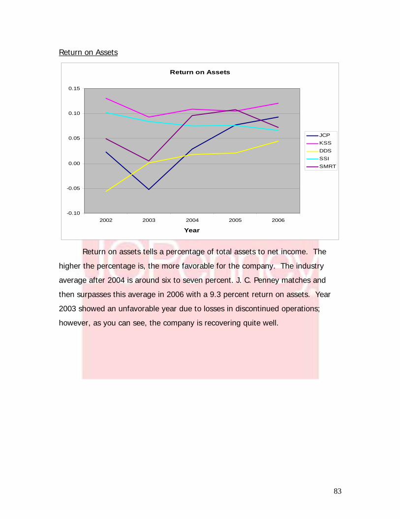
83

Return on Assets

Return on Assets

-0.10

-0.05

0.00

0.05

0.10

0.15

2002 2003 2004 2005 2006

Year

JCPKSSDDSSSISMRT

Return on assets tells a percentage of total assets to net income. The

higher the percentage is, the more favorable for the company. The industry

average after 2004 is around six to seven percent. J. C. Penney matches and

then surpasses this average in 2006 with a 9.3 percent return on assets. Year

2003 showed an unfavorable year due to losses in discontinued operations;

however, as you can see, the company is recovering quite well.

84

Return on Equity

Return on Equity

-0.20

-0.15

-0.10

-0.05

0.00

0.05

0.10

0.15

0.20

0.25

0.30

0.35

2002 2003 2004 2005 2006

Year

JCPKSSDDSSSISMRT

Return on equity shows that for every dollar of equity, a company has X

amount of net income. Looking at the industry, from 2003 to 2006, there is a

rise in this ratio across the board. J. C. Penney especially shows improvement,

once more, due to the fact of sales of unprofitable companies in 2004. After the

fact of these sales, the company then rises above the industry to a very

favorable 28 percent.

Conclusion

After assessing all profitability ratios, J. C. Penney, compared to the

industry, is follow trend very well. After 2003, the company shows

improvements in all areas with the exception of asset turnover. All of this can be

attributed to the sale of Rojas Renner S. A. and Eckerd Pharmacy in 2003 and

2004, respectively. Not only does the company show improvements, but they

also surpass averages in almost all areas. This shows that J. C. Penney is

improving in profitability as they push forward into the future.

85

Capital Structure Analysis

When looking at capital structure ratios, the emphasis is on ability of a

company to meet debt obligations in relation to owner’s equity. The debt to

equity, times interest earned, and debt service margin ratios explain where a

company stands in this respect. The following analysis compares the J. C.

Penney Company to the rest of the industry.

Debt to Equity

Debt to Equity Ratio

0.0

0.5

1.0

1.5

2.0

2.5

3.0

3.5

4.0

4.5

2002 2003 2004 2005 2006

Year

JCPKSSDDSSSISMRT

The debt to equity ratio shows how much debt a company has compared

to equity. For every dollar in equity, this ratio shows how much debt a company

has. The industry shows a fair average of debt to equity between .5 and 1.75. J.

C. Penney and Dillard’s have high debt to equity compared to Stein Mart, Kohl’s,

and Stage Stores widely ranging roughly from 1.75 all the way to 4.2. The

Dillard’s Company is having problems over the years dealing with restructuring,

so this company has been all over the charts on most comparisons. Therefore,

J. C. Penney compared to the industry has an unfavorable record of debt to

86

equity. As we follow the trend through the years, you can see the impact of the

sale of Eckerd Pharmacy in 2004. Debt dropped, bringing the ratio down, but

due to a push in change in brand lines and differentiation, the ratio rises again.

Times Interest Earned

Times Interest Earned

-55

-45

-35

-25

-15

-5

5

15

25

35

45

55

2002 2003 2004 2005 2006

Year

JCPKSSDDSSSISMRT

Time interest earned ratio tells that for every dollar in interest expense,

the company has this amount in NIBIT to spend on interest and taxes. The

industry numbers run around 2-15 times interest payable to NIBIT. In 2004,

Stein Mart’s times interest earned suddenly shot up because it reported net

interest income of $332,000 compared to interest expense of $1.7 million for

2003. As a result of increased sales, decreased inventories, and ongoing

expense control, Stein Mart has not borrowed on its revolving credit agreement

since the first quarter of 2004, completely eliminating its interest expense (Stein

Mart 2004 10-K).

J. C. Penney is unfavorable with this ratio. As we look at years 2003-

2005, the company shows a negative times interest earned. This says that in

these years, the company did not earn enough to cover their interest expenses;

87

however, in 2006, J. C. Penney showed improvements with a ratio of 14.78,

coming closer to the industry average.

Debt Service Margin

Debt Service Margin

-100

100

300

500

700

900

1100

1300

1500

1700

2002 2003 2004 2005 2006

Year

JCPKSSDDSSSISMRT

The debt service margin ratio explains how well the company covers their

debt service with cash flows created through operations. The industry average is

fairly consistently low, when leaving out the obvious outlier, Stage Stores, Inc.,

which maintains substantially lower levels of long-term debt. This tells us that

the industry is able to fund the cash for current notes payable but, on average,

with little cash left at the end of the year. The debt service margin trend for J.

C. Penney is low compared to other companies; the company barely covers

current notes payable. A higher margin would of course be better for the

company.

Conclusion

After reviewing the capital structure ratios of the J. C. Penney Company

compared to industry averages, the company mostly follows the trend of the

88

industry. Unfavorable numbers present in the debt to equity ratio as well as

times interest earned ratio compared to industry averages; although, fluctuation

is higher in at least one other company in both aspects. Because of these

reasons, the company does not raise any red flags, but it also shows that the

J. C. Penney is not an industry leader in respect to the ability to pay debts with

shareholder’s equity. This is found to be caused by the investments in

restructuring after the sales of Eckerd Pharmacy and Rojas Renner S. A. as well

as the push of new brands and labels by the company.

IGR/SGR Analysis

Determining a firm’s estimated growth rates helps paint a picture of

whether or not they will continue to be profitable in the future. The growth rate

of a firm is dependent upon a number of factors including their returns on assets

and equity, as well as their dividend payout and debt to equity ratios.

Internal Growth Rate

A firm’s internal growth rate (IGR) determines how much a company can

grow their asset base that can be sustained all with internal financing. This

means that the firm is trying to increase their assets without financing them with

debt. They are trying to finance future projects completely with funds generated

from the firms operations and not borrow any excessive amounts of funding from

banks or any kind of financial institutions. J. C. Penney has a relatively small IGR

compared to firms such as Kohl’s and Stage Stores, Inc. They are obviously

funding more of their future projects with borrowed versus internally generated

funding than these competitors. However, their IGR is higher than that of

Dillard’s, so they are funding less of their future projects with debt and more

with internal funds. J. C. Penney’s IGR is pretty consistent with that of Stein

Mart. They both are keeping a steady balance between funding with debt and

internal financing.

89

Sustainable Growth Rate

Sustainable growth rate (SGR) is the maximum rate of growth that a firm

can achieve without adding additional debt. If a firm exceeds this limit they will

have to increase their financial leverage by borrowing more funds to maintain

this level of growth. Since SGR is determined based on the company’s internal

growth rate, J. C. Penney holds the same amount of sustainable growth as it did

with IGR compared to its competition. They have a small SGR compared to

Kohl’s and Stage Stores, Inc. and a higher SGR than Dillard’s. They stay

constant with Stein Mart meaning that they are increasing their financial leverage

at about the same rate.

IGR & SGR Analysis

-0.20

-0.10

0.00

0.10

0.20

0.30

0.40

2002 2003 2004 2005 2006

Year

JCP IGRAverage IGRJCPAverage SGR

J. C. Penney’s internal and sustainable growth rates determine the

amount of debt they will increase for funding of future projects. These are

important ratios because they determine the level of future profitability of the

company. When the firm increases their financial leverage by acquiring more

debt for financing, they will inadvertently reduce the level of future profitability

because they have increased future financial obligations to pay. If the IGR and

SGR ratios are higher, then they will have fewer obligations and therefore will be

90

more profitable in the future. Since J. C. Penney’s IGR and SGR are a relatively

small compared to their competitors, it explains that they are in the process of

acquiring more debt than these other companies acquire. This is probably

because they are currently maintaining an aggressive growth plan. Once this

plan is complete, they will have the ability to increase these numbers thus

maintaining a higher level of profitability.

Financial Statement Forecasting

Financial statement forecast analysis is a process designed to provide

insight into the actual valuation of a firm. It estimates a firm’s future value

based on historical financial statements given in a firm’s annual 10-K reports.

We assumed the sustainability of J. C. Penney’s productivity performance based

on the annual filings over the past five years. Based on these assumptions, we

forecasted J. C. Penney’s income statement, balance sheet, and statement of

cash flows for the next 10 years. To forecast the income statement, we based

our assumptions on a mix of J. C. Penney’s historical average growth rates and

those of the industry. When forecasting the balance sheet, we utilized not only

growth rates but also accounts receivable turnover, inventory turnover, asset

turnover, and current ratios for J. C. Penney. We then used the manipulation

diagnostics for core expenses in relation to CFFO to base our assumptions for the

statement of cash flows. These ratios are CFFO/OI and CFFO/NI.

Income statement Analysis

To forecast the income statement, we looked at the financials in many

different aspects. First, we found the average percentages of all line items

compared to net sales. Some of this information was found irrelevant because of

many industry fluctuations on the years 2002 and 2003. In addition, because J.

C. Penney sold Eckerd in April of 2004, we decided that 2004 did not give a fair

view of the future of the financials. Because of these deficiencies, we took an

91

average of only years 2005 and 2006 for J. C. Penney and started from there.

This two-year average seemed like a very reasonable starting point, but because

only two years were used to average out future potential of the income

statement, we did an industry average which included J. C. Penney as well as

four other competitors. This industry average, compared to J. C. Penney’s

relevant two-year average, gave a jump-start to how we decided on which

values to use in forecasting the next 10 years.

Going through the income statement, all line items that could be

appropriately forecasted were considered. Because of the company turn-around

after 2004, as well as new brand launches, we went for a percentage that was

higher than J. C. Penney historical two-year average of 3.96 percent. After

benchmarking this with industry average of 9.52 percent, we found that a 6.00

percent growth rate was fair and very reasonable. From year 2006 to 2007,

sales forecasted grew from a published $19,903 million to $21,097 million. This

6 percent growth percentage is lower than the industry average; however, we

felt like this is an appropriate number considering Stage Stores had a higher than

normal growth rate, therefore raising the overall average. This high rate was

because Stage Stores opened more new stores over the last year than most

firms in the industry.

The cost of goods sold was determined to also be lower than not only the

industry average, 67.82 percent, but also the J. C. Penney five year averages,

63.05 percent. This again is due to the fact of the company sold by J. C. Penney

in 2004. After this, sales and cost of sales went down for obvious reasons. The

two-year relevant average came to 60.71 percent. Looking at all of these

numbers, we chose a number higher than our two-year average to match the

increase in sales of 61.00 percent. It is higher because as sales increase every

year, the cost of sales will be a higher number in the long run.

For the remainder of the forecasted line items, comparisons between the

industry, J. C. Penney five-year, and J. C. Penney two-year averages were

considered just as in sales and cost of sales for the values chosen. We felt that

92

our predicted future values show optimism for steady growth over the next 10

years because of the analysis of the forward-looking vision of the company itself.

93

(reported in millions)Annual Income Statement 2002 2003 2004 2005 2006 Average Avg 05-06 Ind. Avg. Assumed 2007 2008 2009 2010 2011 2012 2013 2014 2015 2016

Retail sales, net $32,347 $17,786 $18,424 $18,781 $19,903 100.00% 100.00% 100.00% 6.00% $21,097 $22,363 $23,705 $25,127 $26,635 $28,233 $29,927 $31,722 $33,626 $35,643Cost of goods sold $22,573 $11,166 $11,285 $11,405 $12,078 -6.49% 3.96% 9.52% 61.00% $12,869 $13,641 $14,460 $15,328 $16,247 $17,222 $18,255 $19,351 $20,512 $21,742Gross margin $9,774 $6,620 $7,139 $7,376 $7,825 63.05% 60.71% 67.82% 39.00% $8,228 $8,722 $9,245 $9,800 $10,388 $11,011 $11,671 $12,372 $13,114 $13,901Selling, general & administrative expenses $8,667 $5,830 $5,827 $5,799 $5,521 36.95% 39.29% 32.81% 29.25% $6,171 $6,541 $6,934 $7,350 $7,791 $8,258 $8,754 $9,279 $9,836 $10,426Total operating expenses $8,667 $5,830 $5,827 $5,799 $5,903 30.35% 30.27% 26.69% 30.25% $6,382 $6,765 $7,171 $7,601 $8,057 $8,540 $9,053 $9,596 $10,172 $10,782Operating income $1,107 $790 $1,312 $1,577 $1,922 6.61% 9.03% 6.53% 8.75% $1,846 $1,957 $2,074 $2,199 $2,331 $2,470 $2,619 $2,776 $2,942 $3,119Total costs & expenses $31,763 $17,336 $17,442 $17,403 $18,179 94.87% 92.00% 93.56% 90.50% $19,093 $20,239 $21,453 $22,740 $24,104 $25,551 $27,084 $28,709 $30,431 $32,257Income tax expense $213 $182 $353 $467 $658 1.88% 2.90% 2.05% 3.50% $738 $783 $830 $879 $932 $988 $1,047 $1,110 $1,177 $1,248Net income (loss) $405 ($928) $524 $1,088 $1,153 2.09% 5.79% 3.13% 6.00% $1,266 $1,342 $1,422 $1,508 $1,598 $1,694 $1,796 $1,903 $2,018 $2,139

Common Size Income Statement 2002 2003 2004 2005 2006 Average Avg 05-06 Ind. Avg. Assumed 2007 2008 2009 2010 2011 2012 2013 2014 2015 2016

Sales Growth Percent 1.07% -45.01% 3.59% 1.94% 5.97% -6.49% 3.96% 9.52% 6.00% 6.00% 6.00% 6.00% 6.00% 6.00% 6.00% 6.00% 6.00% 6.00% 6.00%Cost of goods sold 69.78% 62.78% 61.25% 60.73% 60.68% 63.05% 60.71% 67.82% 61.00% 61.00% 61.00% 61.00% 61.00% 61.00% 61.00% 61.00% 61.00% 61.00% 61.00%Gross margin 30.22% 37.22% 38.75% 39.27% 39.32% 36.95% 39.29% 32.81% 39.00% 39.00% 39.00% 39.00% 39.00% 39.00% 39.00% 39.00% 39.00% 39.00% 39.00%Selling, general & administrative expenses 26.79% 32.78% 31.63% 30.88% 27.74% 29.96% 29.31% 24.87% 29.25% 29.25% 29.25% 29.25% 29.25% 29.25% 29.25% 29.25% 29.25% 29.25% 29.25%Total operating expenses 26.79% 32.78% 31.63% 30.88% 29.66% 30.35% 30.27% 26.69% 31.00% 31.00% 31.00% 31.00% 31.00% 31.00% 31.00% 31.00% 31.00% 31.00% 31.00%Operating income 3.42% 4.44% 7.12% 8.40% 9.66% 6.61% 9.03% 6.53% 10.00% 10.00% 10.00% 10.00% 10.00% 10.00% 10.00% 10.00% 10.00% 10.00% 10.00%Total costs & expenses 98.19% 97.47% 94.67% 92.66% 91.34% 94.87% 92.00% 93.56% 90.50% 90.50% 90.50% 90.50% 90.50% 90.50% 90.50% 90.50% 90.50% 90.50% 90.50%Income tax expense 0.66% 1.02% 1.92% 2.49% 3.31% 1.88% 2.90% 2.05% 3.50% 3.50% 3.50% 3.50% 3.50% 3.50% 3.50% 3.50% 3.50% 3.50% 3.50%Net income (loss) 1.25% -5.22% 2.84% 5.79% 5.79% 2.09% 5.79% 3.13% 6.00% 6.00% 6.00% 6.00% 6.00% 6.00% 6.00% 6.00% 6.00% 6.00% 6.00%

94

Balance Sheet Analysis

When determining the future profitability of J. C. Penney, we began by creating a

common-sized balance sheet to get a general idea of how the firm was performing compared to

the industry. We then used the industry averages as a benchmark and compared their numbers

to those of J. C. Penney’s. This aided in the determination of which ratios to utilize in order to

provide us with the best estimations for the forecasting process.

We began by looking at the asset portion of the balance sheet, ultimately deciding that our

total assets line was what we should use to base all of our other asset estimations. This

determination was decided upon because obviously current and non-current assets should be

combined and result in total assets. Looking at the industry average, we agreed that it would not

be the best number to base our assumptions on because our firm is relatively larger than that of

most within the industry and should therefore have more assets.

While looking at our asset turnover, which was determined to be 1.584, we noticed a trend

over the previous two years and decided to use it in comparison to our already forecasted sales

for our income statement analysis. Once we determined our total assets, we then decided upon

the percentage of current and non-current assets based off our forecasted total assets.

Breaking up these two portions, we began analyzing total current assets. We determined

cash and short-term investments to be an average of the previous two years. They were higher

than the industry average because we have continuously been above the industry average.

Because of the fact that our company is larger than others within the retail industry, we agreed

that this was a reasonable number. Accounts receivable turnover was based on the last year and

applied to our forecasted sales from the income statement. We used the most recent A/R

turnover of 75.68 because it was approximately where the industry average should be. The

inventory turnover ratio used was based on the number given for the last year because it was at

a stable level for the previous two to three years. We manipulated this equation to come up with

inventory by using our already forecasted cost of goods sold. Total non-current assets was then

determined based on our estimations of total current assets. Property and equipment was

assumed to be increasing because of the plans for expansion of our company within the next few

years. We are thus converging toward the industry average.

95

We then began to look at the equity portion of the balance sheet. We began by looking at

return on equity. We used an average of the last two years because, compared to the industry,

there seems to be a convergence. We determined that J. C. Penney would remain constant at

the level of 28.77 because of this industry convergence. Retained earnings were determined by

taking the forecasted net income from the income statement and subtracting out the forecasted

dividends. Since we cannot forecast the number of share we will have in the future, we used the

226 million outstanding shares we already have.

We then backed into total liabilities because of how liabilities plus equity equals assets. We

decided that these numbers should balance out. We used the current ratio to determine what our

current liabilities should be. We determined that trade payables should be a little higher than that

of the average found on our common-sized balance sheet. This is because we are increasing at

an incremental level to meet industry average. We decided that the same process and reasoning

should be applied to our gift cards. Once the current liabilities were determined, we began to

analyze our total non-current liabilities. Total accrued expenses have had consistent ratios over

the past five years so we slightly increased it to meet the industry average. Notes payable have

had a consistent percentage of 20 for the past five years. We determined that this percentage

should be kept because once amounts get paid off we will have more notes payable due to our

accelerated growth plan.

96

(reported in millions)Balance Sheet 2002 2003 2004 2005 2006 2007 2008 2009 2010 2011 2012 2013 2014 2015 2016

Cash & short-term investments $2,474 $2,994 $4,687 $3,016 $2,747 $3,056 $3,239 $3,433 $3,639 $3,858 $4,089 $4,335 $4,595 $4,870 $5,163Receivables, net $705 $233 $404 $270 $263 $279 $296 $313 $332 $352 $373 $395 $419 $444 $471Merchandise inventories $4,945 $3,156 $3,169 $3,210 $3,400 $3,623 $3,840 $4,071 $4,315 $4,574 $4,848 $5,139 $5,447 $5,774 $6,121Prepaid expenses $229 $130 $167 $206 $238Total current assets $8,353 $6,513 $8,427 $6,702 $6,648 $7,076 $7,501 $7,951 $8,428 $8,933 $9,469 $10,037 $10,640 $11,278 $11,955

Land & buildings $2,940 $2,760 $2,896 $3,045 $3,378Furniture & fixtures $3,946 $2,203 $2,145 $2,078 $2,104Leasehold improvements $1,268 $674 $674 $722 $795Accumulated depreciation $3,253 $2,122 $2,077 $2,097 $2,115Property & equipment, net $4,901 $3,515 $3,638 $3,748 $4,162 $4,422 $4,695 $4,984 $5,291 $5,617 $5,963 $6,330 $6,720 $7,134 $7,573Prepaid pension - $1,320 $1,538 $1,469 $1,235Goodwill & other intangible assets, net $2,798 $42 - - -Real estate investments $106 $169 $192 $270 $350Leveraged lease investments $131 $134 $139 $135 $140Capitalized software, net $228 $97 $99 $89 $95Goodwill - Renner - - $43 - -Deferred catalog book costs $73 $77 - - -Debt issuance costs, net $46 $52 $31 $24 $21Prepaid pension $1,172 - - - -Other assets $59 $27 $20 $24 $22Total other assets $1,815 $556 $524 $542 $628Assets of discontinued operations - $6,354 - - -Total noncurrent assets $9,514 $11,787 $5,700 $5,759 $6,025 $6,245 $6,619 $7,016 $7,437 $7,884 $8,357 $8,858 $9,390 $9,953 $10,550Total assets $17,867 $18,300 $14,127 $12,461 $12,673 $13,321 $14,120 $14,967 $15,865 $16,817 $17,826 $18,896 $20,029 $21,231 $22,505

Trade payables $1,792 $1,167 $1,200 $1,171 $1,366 $1,440 $1,531 $1,628 $1,730 $1,840 $1,956 $2,079 $2,210 $2,349 $2,497Accrued salaries, vacation & bonus $570 $409 $443 $453 $455Customer gift cards/certificates $173 $179 $207 $219 $231 $243 $255 $268 $282 $296 $312 $328 $346 $365 $384Taxes other than income taxes - - $125 $74 $116Capital expenditures payable - - - $47 $88Interest payable $122 $132 $107 $95 $84Current portion of retirement plan liabilitie - - - - $74Advertising payables $187 $79 $78 $99 $93Current portion of workers' compensation & ge $99 $63 $68 $72 $67Occupancy & rent-related payables $91 - - $51 $46Common dividends payable $34 $35 $35 $29 $41Reserves for discontinued operations - - $221 $79 $34Taxes payable $123 $119 $79 - -Other accrued expenses & other curr liabils $432 $368 $352 $344 $363Total accrued expenses & oth current liabils - - $1,766 $1,562 $1,692 $1,633 $1,731 $1,835 $1,945 $2,062 $2,185 $2,316 $2,455 $2,603 $2,759Accounts payable & accrued expenses $3,791 $2,551 - - -Current maturities of long term debt $275 $242 $459 $21 $434Income taxes payable - - - $8 -Short-term debt $13 $18 $22 - -Deferred taxes $80 $943 - - -Total current liabilities $4,159 $3,754 $3,447 $2,762 $3,492 $3,717 $3,940 $4,176 $4,427 $4,692 $4,974 $5,272 $5,589 $5,924 $6,280

Notes $1,928 $2,165 $1,857 $1,763 $1,763 $1,633 $1,731 $1,835 $1,945 $2,062 $2,185 $2,316 $2,455 $2,603 $2,759Debentures $1,525 $1,525 $1,525 $1,369 $1,369Notes & debentures $3,453 $3,690 $3,382 $3,132 $3,132Medium-term notes $493 $493 $493 $300 $300Convertible subordinated notes $650 $650 - - -Sunking fund debentures $392 $313 - - -Original issue discount debentures $156 $167 - - -Equipment financing notes $25 $21 $15 $10 $4Total notes & debentures - - $3,890 $3,442 $3,436Capital lease obligs & other long-term debt $46 $22 $33 $23 $8Total long-term debt, including current matur - - $3,923 $3,465 $3,444Less: current maturities $275 $242 $459 $21 $434Long-term debt $4,940 $5,114 $3,464 $3,444 $3,010Deferred taxes $1,391 $1,217 $1,318 $1,287 $1,206Retirement benefit plan liabilities - - $634 $590 $324Reserves for discontinued operations - - $114 $54 $51Other liabilities $1,007 $804 $26 $31 $30Total other liabilities - - $1,042 $961 $677Liabilities of discontinued operations - $1,986 - - -Total NonCurrent Liabilities $7,338 $9,121 $5,824 $5,692 $4,893 $4,657 $4,937 $5,233 $5,547 $5,880 $6,232 $6,606 $7,003 $7,423 $7,868Total liabilities $11,497 $12,875 $9,271 $8,454 $8,385 $8,374 $8,876 $9,409 $9,974 $10,572 $11,206 $11,879 $12,591 $13,347 $14,148

Preferred stock $333 $304 - - -Common stock & additional paid-in capital $3,423 $3,531 $4,176 $3,479 $3,542Deferred stock compensation - - - - -Reinvested earnings $2,817 $1,728 $812 $512 $922 $1,085 $1,161 $1,241 $1,306 $1,396 $1,492 $1,572 $1,679 $1,794 $1,915Foreign currency translation ($164) ($115) ($104) - -Non-qualified plan minimum liability adjustme ($58) ($82) ($102) ($102) -Net unrealized gains on investments $19 $60 $74 $118 $166Net actuarial gain/(loss) & prior service (co - - - - ($342)Other comprehensive (loss) from discont opers - ($1) - - -Accumulated other comprehensive income (loss) ($203) ($138) ($132) $16 ($176)Total stockholders' equity $6,370 $5,425 $4,856 $4,007 $4,288 $4,947 $5,243 $5,558 $5,891 $6,245 $6,620 $7,017 $7,438 $7,884 $8,357

97

Common Size Balance Sheet 2002 2003 2004 2005 2006 AVGAVG 05-06

Industry Average Assumed

Cash & short-term investments 13.85% 16.36% 33.18% 24.20% 21.68% 21.85% 22.94% 10.68% 22.94%Receivables, net 3.95% 1.27% 2.86% 2.17% 2.08% 2.46% 2.12% 4.31% 75.68Merchandise inventories 27.68% 17.25% 22.43% 25.76% 26.83% 23.99% 26.29% 36.03% 3.552Prepaid expenses 1.28% 0.71% 1.18% 1.65% 1.88% 1.34% 1.77%Total current assets 46.75% 35.59% 59.65% 53.78% 52.46% 49.65% 53.12% 52.07% 53.12%

Land & buildings 16.45% 15.08% 20.50% 24.44% 26.66% 20.63% 25.55%Furniture & fixtures 22.09% 12.04% 15.18% 16.68% 16.60% 16.52% 16.64%Leasehold improvements 7.10% 3.68% 4.77% 5.79% 6.27% 5.52% 6.03%Accumulated depreciation 18.21% 11.60% 14.70% 16.83% 16.69% 15.60% 16.76%Property & equipment, net 27.43% 19.21% 25.75% 30.08% 32.84% 27.06% 31.46% 42.61% 33.20%Prepaid pension 0.00% 7.21% 10.89% 11.79% 9.75% 7.93% 10.77%Goodwill & other intangible assets, net 15.66% 0.23% 0.00% 0.00% 0.00% 3.18% 0.00%Real estate investments 0.59% 0.92% 1.36% 2.17% 2.76% 1.56% 2.46%Leveraged lease investments 0.73% 0.73% 0.98% 1.08% 1.10% 0.93% 1.09%Capitalized software, net 1.28% 0.53% 0.70% 0.71% 0.75% 0.79% 0.73%Goodwill - Renner 0.00% 0.00% 0.30% 0.00% 0.00% 0.06% 0.00%Deferred catalog book costs 0.41% 0.42% 0.00% 0.00% 0.00% 0.17% 0.00%Debt issuance costs, net 0.26% 0.28% 0.22% 0.19% 0.17% 0.22% 0.18%Prepaid pension 6.56% 0.00% 0.00% 0.00% 0.00% 1.31% 0.00%Other assets 0.33% 0.15% 0.14% 0.19% 0.17% 0.20% 0.18%Total other assets 10.16% 3.04% 3.71% 4.35% 4.96% 5.24% 4.65%Assets of discontinued operations 0.00% 34.72% 0.00% 0.00% 0.00% 6.94% 0.00%Total noncurrent assets 53.25% 64.41% 40.35% 46.22% 47.54% 50.35% 46.88% 47.60%Total assets 100.00% 100.00% 100.00% 100.00% 100.00% 100.00% 100.00% 1.584

Trade payables 15.59% 9.06% 12.94% 13.85% 16.29% 13.55% 15.07% 26.14% 17.20%Accrued salaries, vacation & bonus 4.96% 3.18% 4.78% 5.36% 5.43% 4.74% 5.39%Customer gift cards/certificates 1.50% 1.39% 2.23% 2.59% 2.75% 2.09% 2.67% 5.63% 5%Taxes other than income taxes 0.00% 0.00% 1.35% 0.88% 1.38% 0.72% 1.13%Capital expenditures payable 0.00% 0.00% 0.00% 0.56% 1.05% 0.32% 0.80%Interest payable 1.06% 1.03% 1.15% 1.12% 1.00% 1.07% 1.06%Current portion of retirement plan liabilitie 0.00% 0.00% 0.00% 0.00% 0.88% 0.18% 0.44%Advertising payables 1.63% 0.61% 0.84% 1.17% 1.11% 1.07% 1.14%Current portion of workers' compensation & ge 0.86% 0.49% 0.73% 0.85% 0.80% 0.75% 0.83%Occupancy & rent-related payables 0.79% 0.00% 0.00% 0.60% 0.55% 0.39% 0.58%Common dividends payable 0.30% 0.27% 0.38% 0.34% 0.49% 0.36% 0.42%Reserves for discontinued operations 0.00% 0.00% 2.38% 0.93% 0.41% 0.74% 0.67%Taxes payable 1.07% 0.92% 0.85% 0.00% 0.00% 0.57% 0.00%Pharmacy payables 1.14% 0.00% 0.00% 0.00% 0.00% 0.23% 0.00%Restructuring reserves 0.32% 0.00% 0.00% 0.00% 0.00% 0.06% 0.00%Funds due for common stock repurchases 0.00% 0.00% 0.55% 0.00% 0.00% 0.11% 0.00%Other accrued expenses & other curr liabils 3.76% 2.86% 3.80% 4.07% 4.33% 3.76% 4.20%Total accrued expenses & oth current liabils 0.00% 0.00% 19.05% 18.48% 20.18% 19.23% 19.33% 25.69% 19.50%Accounts payable & accrued expenses 32.97% 19.81% 0.00% 0.00% 0.00% 10.56% 0.00%Current maturities of long term debt 2.39% 1.88% 4.95% 0.25% 5.18% 2.93% 2.71%Income taxes payable 0.00% 0.00% 0.00% 0.09% 0.00% 0.02% 0.05%Short-term debt 0.11% 0.14% 0.24% 0.00% 0.00% 0.10% 0.00%Deferred taxes 0.70% 7.32% 0.00% 0.00% 0.00% 1.60% 0.00%Total current liabilities 36.17% 29.16% 37.18% 32.67% 41.65% 35.37% 37.16% 52.76% 2.100

Notes 16.77% 16.82% 20.03% 20.85% 21.03% 19.10% 20.94% 12.16% 20.00%Debentures 13.26% 11.84% 16.45% 16.19% 16.33% 14.82% 16.26%Notes & debentures 30.03% 28.66% 36.48% 37.05% 37.35% 33.91% 37.20% 23.61%Medium-term notes 4.29% 3.83% 5.32% 3.55% 3.58% 4.11% 3.56%Convertible subordinated notes 5.65% 5.05% 0.00% 0.00% 0.00% 2.14% 0.00%Sunking fund debentures 3.41% 2.43% 0.00% 0.00% 0.00% 1.17% 0.00%Original issue discount debentures 1.36% 1.30% 0.00% 0.00% 0.00% 0.53% 0.00%Equipment financing notes 0.22% 0.16% 0.16% 0.12% 0.05% 0.14% 0.08%Total notes & debentures 0.00% 0.00% 41.96% 40.71% 40.98% 24.73% 40.85%Capital lease obligs & other long-term debt 0.40% 0.17% 0.36% 0.27% 0.10% 0.26% 0.18%Total long-term debt, including current matur 0.00% 0.00% 42.31% 40.99% 41.07% 24.87% 41.03%Less: current maturities 2.39% 1.88% 4.95% 0.25% 5.18% 2.93% 2.71%Long-term debt 42.97% 39.72% 37.36% 40.74% 35.90% 39.34% 38.32%Deferred taxes 12.10% 9.45% 14.22% 15.22% 14.38% 13.07% 14.80%Retirement benefit plan liabilities 0.00% 0.00% 6.84% 6.98% 3.86% 3.54% 5.42%Long-term portion of workers' compensation & 0.00% 0.00% 1.69% 1.94% 1.81% 1.09% 1.88%Developer/tenant allowances 0.00% 0.00% 1.20% 1.44% 1.43% 0.81% 1.44%Reserves for discontinued operations 0.00% 0.00% 1.23% 0.64% 0.61% 0.50% 0.62%Other liabilities 0.00% 0.00% 0.28% 0.37% 0.36% 0.20% 0.36%Total other liabilities 0.00% 0.00% 11.24% 11.37% 8.07% 6.14% 9.72%Liabilities of discontinued operations 0.00% 15.43% 0.00% 0.00% 0.00% 3.09% 0.00%Total NonCurrent Liabilities 63.83% 70.84% 62.82% 67.33% 58.35% 64.63% 62.84% 46.85%Total liabilities 100.00% 100.00% 100.00% 100.00% 100.00% 100.00% 100.00%

Preferred stock 5.23% 5.60% 0.00% 0.00% 0.00% 2.17% 0.00%Common stock & additional paid-in capital 53.74% 65.09% 86.00% 86.82% 82.60% 74.85% 84.71%Deferred stock compensation 0.00% 0.00% 0.00% 0.00% 0.00% 0.00% 0.00%Reinvested earnings 44.22% 31.85% 16.72% 12.78% 21.50% 25.42% 17.14% 63.96% 25%Foreign currency translation -2.57% -2.12% -2.14% 0.00% 0.00% -1.37% 0.00%Non-qualified plan minimum liability adjustme -0.91% -1.51% -2.10% -2.55% 0.00% -1.41% -1.27%Net unrealized gains on investments 0.30% 1.11% 1.52% 2.94% 3.87% 1.95% 3.41%Net actuarial gain/(loss) & prior service (co 0.00% 0.00% 0.00% 0.00% -7.98% -1.60% -3.99%Other comprehensive (loss) from discont opers 0.00% -0.02% 0.00% 0.00% 0.00% 0.00% 0.00%Accumulated other comprehensive income (loss) -3.19% -2.54% -2.72% 0.40% -4.10% -2.43% -1.85%Total stockholders' equity 100.00% 100.00% 100.00% 100.00% 100.00% 100.00% 100.00%

98

Statement of Cash Flow Analysis We began the forecasting process by common sizing the cash flow

statement to see if there were any patterns. We noticed net income had a

consistent trend unlike the rest of the numbers within the statement. We

proceeded by manipulating the following ratios: CFFO/NI, CFFO/OI, CFFO/Sales,

and CFFO/Gross Profit. After looking to find patterns in the numbers, we opted

to forecast using the CFFO/NI and CFFO/Sales. We forecasted CFFO by using

the previously forecasted sales numbers from the income statement. Then we

continued by using the forecasted cash flows to calculate net income with the

CFFO/NI ratio. After looking at the forecasted net income and operating cash

flows, we recognized a trend between the previous cash flow statements. This

perceived trend proved good logic in our justification. We forecasted the CFFI

activities using our estimates of changes in PP&E. This proved to be a more

effective measure of the growth of Total Assets because the Balance Sheet

estimate contained misleading items like Capitalized Software and a poorly

defined Other Assets section.

99

(numbers in millions)

Statement of Cash Flows 2002 2003 2004 2005 2006 2007 2008 2009 2010 2011 2012 2013 2014 2015 2016

Net income (loss) $371 $364 $667 $1,088 $1,153 $1,220 $1,293 $1,371 $1,453 $1,540 $1,633 $1,731 $1,834 $1,944 $2,061Loss (income) from discontinued operations - - - ($111) ($19)Asset impair, PVOL & other unit closing costs $104 $35 $19 $12 $4Restructuring & other charges, net - - - - -Depreciation & amortization $667 $394 $368 $372 $389Net gains on sale of assets ($18) ($51) ($8) ($27) ($8)Real estate (gain) - - - - -Co contributions to savings & profits sharing $47 - - - -Benefit plans expense (income) $30 $135 $45 $49 ($51)Pension contribution ($300) ($300) ($300) - ($300)Stock-based compensation $4 $9 $23 $38 $60Tax benefits on stock options exercised - - - - $6Deferred stock compensation - - - - -Deferred taxes $141 $137 $1 $15 ($6)Receivables ($6) $3 ($34) ($44) $29Sale of drugstore receivables - - - - -Other receivables - - - - -Inventory $82 ($100) ($13) ($67) ($190)Prepaid expenses & other assets ($36) ($36) $9 ($16) ($37)Other assets - - - - -Accounts payable $138 - $33 - -Trade payables - - - $28 $195Accounts payable & accrued expenses - $94 - - -Current income taxes payable $3 ($17) $182 ($124) ($1)Accrued expenses & other liabilities - - $135 $124 $31Other liabilities $102 $145 - - -Net cash flows from operating activities $1,329 $812 $1,127 $1,337 $1,255 $1,414 $1,498 $1,588 $1,684 $1,785 $1,892 $2,005 $2,125 $2,253 $2,388Cash Flows From Investments ($277) ($239) $4,302 ($221) ($752) ($260) ($272) ($289) ($307) ($326) ($346) ($367) ($390) ($414) ($439)

100

Common Size Cash Flow Statement 2002 2003 2004 2005 2006 AVG AVG 05-06

Net income (loss) 27.92% 44.83% 59.18% 81.38% 91.87% 61.04% 86.62%Loss (income) from discontinued operations 0.00% 0.00% 0.00% -8.30% -1.51% -4.91% -4.91%Asset impair, PVOL & other unit closing costs 7.83% 4.31% 1.69% 0.90% 0.32% 3.01% 0.61%Restructuring & other charges, net 0.00% 0.00% 0.00% 0.00% 0.00% 0.00% 0.00%Depreciation & amortization 50.19% 48.52% 32.65% 27.82% 31.00% 38.04% 29.41%Net gains on sale of assets -1.35% -6.28% -0.71% -2.02% -0.64% -2.20% -1.33%Real estate (gain) 0.00% 0.00% 0.00% 0.00% 0.00% 0.00% 0.00%Co contributions to savings & profits sharing 3.54% 0.00% 0.00% 0.00% 0.00% 0.71% 0.00%Benefit plans expense (income) 2.26% 16.63% 3.99% 3.66% -4.06% 4.50% -0.20%Pension contribution -22.57% -36.95% -26.62% 0.00% -23.90% -22.01% -11.95%Stock-based compensation 0.30% 1.11% 2.04% 2.84% 4.78% 2.21% 3.81%Tax benefits on stock options exercised 0.00% 0.00% 0.00% 0.00% 0.48% 0.10% 0.24%Deferred stock compensation 0.00% 0.00% 0.00% 0.00% 0.00% 0.00% 0.00%Deferred taxes 10.61% 16.87% 0.09% 1.12% -0.48% 5.64% 0.32%Receivables -0.45% 0.37% -3.02% -3.29% 2.31% -0.82% -0.49%Sale of drugstore receivables 0.00% 0.00% 0.00% 0.00% 0.00% 0.00% 0.00%Other receivables 0.00% 0.00% 0.00% 0.00% 0.00% 0.00% 0.00%Inventory 6.17% -12.32% -1.15% -5.01% -15.14% -5.49% -10.08%Prepaid expenses & other assets -2.71% -4.43% 0.80% -1.20% -2.95% -2.10% -2.07%Other assets 0.00% 0.00% 0.00% 0.00% 0.00% 0.00% 0.00%Accounts payable 10.38% 0.00% 2.93% 0.00% 0.00% 2.66% 0.00%Trade payables 0.00% 0.00% 0.00% 2.09% 15.54% 3.53% 8.82%Accounts payable & accrued expenses 0.00% 11.58% 0.00% 0.00% 0.00% 2.32% 0.00%Current income taxes payable 0.23% -2.09% 16.15% -9.27% -0.08% 0.99% -4.68%Accrued expenses & other liabilities 0.00% 0.00% 11.98% 9.27% 2.47% 4.74% 5.87%Other liabilities 7.67% 17.86% 0.00% 0.00% 0.00% 5.11% 0.00%Net cash flows from operating activities 100.00% 100.00% 100.00% 100.00% 100.00% 100.00% 100.00%

101

Conclusion

Overall, it appears that J. C. Penney’s productivity is beginning to

converge with that of the industry averages. Although the company took a “big

bath” in 2004 with the selling of Eckerd therefore decreasing their asset base,

they have begun to make a comeback. They are maintaining constant levels of

growth while decreasing their total liabilities and increasing their equity. This

gives us confidence in our future predictions and optimism that J. C. Penney will

continue to grow and prosper within the next ten years.

102

Analysis of Valuations

There are several valuation methods that can be used to derive the share

price of a company. Some of these methods are more accurate than others

because some are derived through theory while others are quick screening

methods. The method of comparables helps us take a quick glance at the share

price relative to the industry average. Based on this data, we can draw

immediate conclusions as to whether our company is overvalued, fairly valued,

or undervalued. The intrinsic valuation models, on the other hand, help us come

up with a more reliable share price that can be used to more accurately value

the firm. Using these valuations, we weighted the several methods from most

accurate to least accurate to come up with a specific share price that we believe

to show a more realistic picture.

Method of Comparables

Price Trailing P/E: $80.34 Forward P/E: $75.64 P.E.G.: $42.55 P/B: $39.62 P/EBITDA: $21.90 P/FCF: N/A* EV/EBITDA: $72.17

The method of comparables is a way to value a company by computing its

share price based upon industry averages. It does so by comparing the firm’s

ratios with industry average ratios. We first took J. C. Penney’s financial data

used for these ratios and put them into a per share basis. We then did the same

for its competitors. By calculating each ratio, we derived an industry average

based on the ratios computed for Dillard’s, Kohl’s, Stein Mart, and Stage Stores,

103

Inc. We set these averages equal to our computed ratios for J. C. Penney to get

a price per share based on each one. The following are the results of this

process.

Forward Price to Earnings

PPS EPS P/E Industry

Average

JCP Share

Price

JCP 81.99 11.30 7.26 15.04 75.64

KSS 70.27 4.51 15.58

DDS 34.62 1.84 18.82

SSI 21.02 1.66 12.66

SMRT 12.57 .96 13.09

This method uses our computed forecasted earnings per share (EPS) and

the current price per share (PPS) reported on June 1, 2007 to derive a P/E ratio

for J.C. Penney. We then took each of our competitors listed prices per share

and their projected earnings per share to get each of their P/E ratios as well.

These numbers were taken from yahoo finance for simplicity purposes. An

industry average was computed by taking the summation of each of our

competitors P/E ratios and dividing that number by four (the number of

competitors listed within our industry). After getting an industry average of

15.04, we multiplied it by J. C. Penney’s forecasted EPS of 11.30 in order to

come up with an estimated price per share for our company. This number was

determined to be $75.64. Based on this method, J. C. Penney appears to be

slightly overvalued when comparing this number to our actual PPS of $81.99.

However, since J. C. Penney’s P/E ratio is ultimately lower than the computed

industry average P/E, this implies that the company still has room for future

earnings growth.

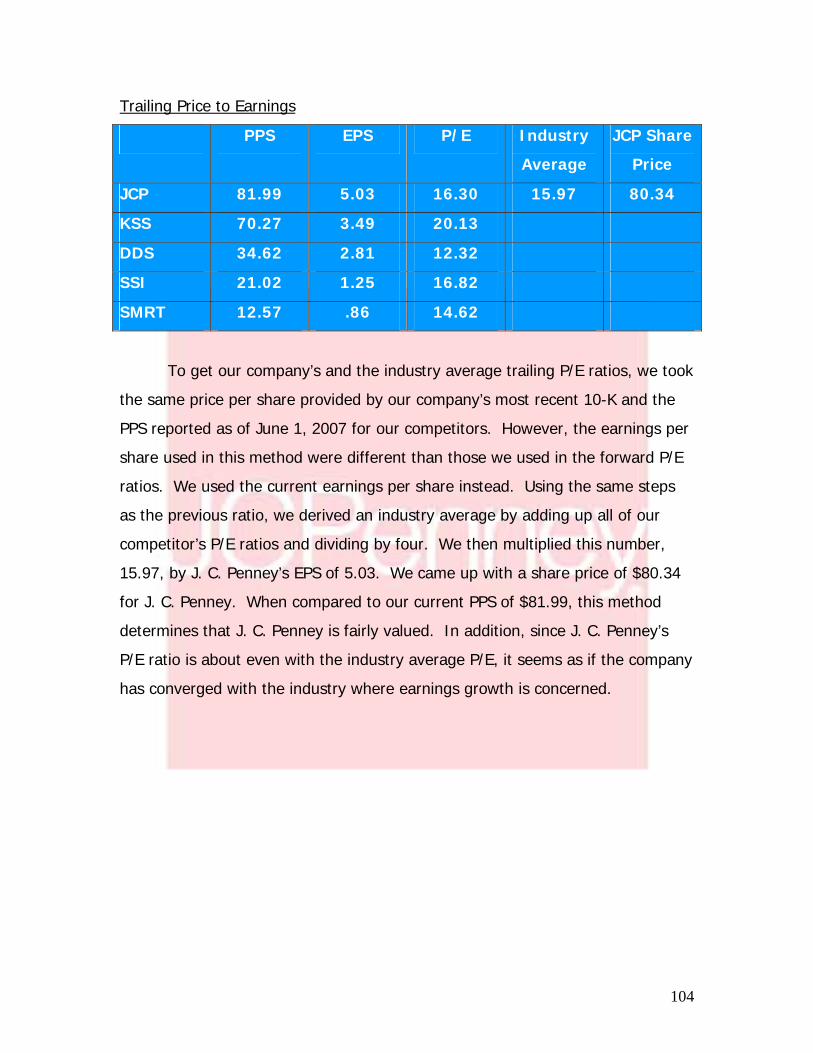
104

Trailing Price to Earnings

PPS EPS P/E Industry

Average

JCP Share

Price

JCP 81.99 5.03 16.30 15.97 80.34

KSS 70.27 3.49 20.13

DDS 34.62 2.81 12.32

SSI 21.02 1.25 16.82

SMRT 12.57 .86 14.62

To get our company’s and the industry average trailing P/E ratios, we took

the same price per share provided by our company’s most recent 10-K and the

PPS reported as of June 1, 2007 for our competitors. However, the earnings per

share used in this method were different than those we used in the forward P/E

ratios. We used the current earnings per share instead. Using the same steps

as the previous ratio, we derived an industry average by adding up all of our

competitor’s P/E ratios and dividing by four. We then multiplied this number,

15.97, by J. C. Penney’s EPS of 5.03. We came up with a share price of $80.34

for J. C. Penney. When compared to our current PPS of $81.99, this method

determines that J. C. Penney is fairly valued. In addition, since J. C. Penney’s

P/E ratio is about even with the industry average P/E, it seems as if the company

has converged with the industry where earnings growth is concerned.

105

Price to Book

PPS BPS P/B Industry

Average

JCP Share

Price

JCP 81.99 18.99 4.32 2.09 39.62

KSS 70.27 18.32 3.84

DDS 34.62 32.76 1.06

SSI 21.02 13.19 1.59

SMRT 12.57 6.76 1.86

The price to book method of comparables uses the current price per share

and book value of equity per share reported in our most recent annual report.

We derived a P/B ratio for our company by dividing our PPS by our BPS. J. C.

Penney’s P/B ratio is 4.32. We then took the same PPS and the BPS of our

competitors reported on yahoo finance for June 1, 2007. We got an industry

average of 2.09 and multiplied this number by our company’s BPS of 18.99. This

gave us a share price for J. C. Penney of $39.62. When compared to our current

PPS of $81.99, J. C. Penney is overvalued using this method. With the P/B ratio

of our company being higher than the industry average, this also shows that J.

C. Penney is overvalued.

106

Dividend Yield

PPS DPS D/P Industry

Average

JCP Price

per Share

JCP 81.99 .72 .009 .05 14.44

KSS 70.27 N/A N/A

DDS 34.62 .16 .005

SSI 21.02 .12 .006

SMRT 12.57 1.75 .139

The dividend yield method uses the current price per share and divides it

by the dividends per share to get a number for dividends paid in comparison to a

company’s share price. We did this for J. C. Penney and its competitors. Kohl’s

was the only company not included in this method because they do not pay out

dividends. We derived an industry average of .05 by adding up all of our

competitor’s D/P ratios and dividing by three so as to not include Kohl’s in our

estimations. Then we took this industry average and divided it into J. C.

Penney’s DPS to get a share price of $14.44 for the company. This method

shows that J. C. Penney is extremely overvalued with regard to their current

share price. But since there is a high degree of noise in the market when

calculating dividend yields, this number is not a very good indicator of the value

of the firm.

107

Price Earnings Growth

PPS EPS PEG Industry

Average

JCP Price

per Share

JCP 81.99 5.03 2.72 1.41 42.55

KSS 70.27 3.49 .93

DDS 34.62 2.81 3.1

SSI 21.02 1.25 .84

SMRT 12.57 .86 .78

The price earnings growth model uses a company’s P/E ratio and divides it

by its estimated earnings growth rate. To derive a share price for J. C. Penney,

we took an average of our competitor’s PEG ratios, 1.41, and multiplied that

number by our company’s estimated earnings growth rate of 6 percent. We then

multiplied the result by our EPS. We got a share price of $42.55 for J. C.

Penney. Compared to J. C. Penney’s current price per share, we see that the

company is overvalued once again.

Price to EBITDA

PPS EBITDA

(in

Billions)

P/EBITDA Industry

Average

JCP Price

per Share

JCP 81.99 2.311 3.55 9.47 21.90

KSS 70.27 2.320 3.03

DDS 34.62 .625 5.54

SSI 21.02 .145 14.53

SMRT 12.57 .090 14.02

This method uses current share prices and earnings before interest, taxes,

depreciation, and amortization to get a P/EBITDA ratio. We used the share price

108

and EBITDA reported on J. C. Penney’s 2006 10-K. By using yahoo finance, we

also came up with our competitor’s PPS and EBITDA. To get reasonable

numbers, we had to place all of the EBITDAs in decimals according to billions. By

dividing the PPS by the EBITDA for each company, we came up with each

individual P/EBITDA ratio. We then computed an industry average by taking the

sum of the P/EBITDA ratios for J. C. Penney’s competitors and dividing this

number by four. We got an industry average of 9.47. Then we took that

number and multiplied it by J. C. Penney’s EBITDA to get a share price for our

company of $21.90. This number indicates that J. C. Penney is extremely

overvalued when compared to our reported price per share.

Enterprise Value to EBITDA

EV EBITDA

(in

Billions)

EV/EBITDA Industry

Average

JCP Price

per Share

JCP 19.29 2.311 8.34 7.39 72.17

KSS 25.20 2.320 10.86

DDS 3.95 .625 6.32

SSI .92 .145 6.36

SMRT .54 .090 6.02

A company’s enterprise value is its price per share plus its book value of

liabilities minus its cash and cash equivalents. We computed this number for J. C.

Penney to be 19.29. To calculate J. C. Penney’s price per share using this

method, we first derived an industry average of EV/EBITDA. This number was

determined by using the enterprise values of J. C. Penney’s competitors and

dividing them by their respective EBITDA. These numbers were reported on

June 1, 2007 by yahoo finance. We took that total and divided by four to get the

average. When deriving a share price we had to multiply the industry average

109

by J. C. Penney’s EBITDA. Then we subtracted its book value of liabilities,

$3,444, and added its cash, $3,689. These numbers were provided by the

company’s most recent balance sheet. We came up with $16,310.42. By

dividing this number by the total number of shares for J. C. Penney, we

determined that our company’s share price based on this model is $72.17.

Again, when compared to the current share price of $81.99, this company is

overvalued.

Price to Free Cash Flows

To determine the P/FCF ratio, free cash flows must first be computed.

This is simply the summation of cash flow from operations and cash flow from

investing. We would use the same methodology as we did for the other ratios,

trying to derive a share price for our company. However, this ratio is not

effective because J. C. Penney has negative cash flows at this time. We decided

that this ratio would be irrelevant for the determination of share price based on

this information.

Conclusion

It is obvious that by using these methods, J. C. Penney is an overvalued

company. Every share price that we have calculated has been lower than the

industry average with the exception of our trailing P/E ratio. Valuing a company

based on the method of comparables is questionable to say the least. These

methods use information in a way that suggests that these companies are

operated in exactly the same way. In addition, things like their size, capital

structure, and accounting methods are not taken into consideration when

comparing these companies using these methods. Even though these methods

have been acceptable for some time now, we feel that in order to value a firm

properly there must be other methods available. Intrinsic valuations are

methods used that take into account the future possibilities of a firm’s activity.

These methods are discussed in the next sections.

110

Cost of Equity

The cost of equity, Ke, is an estimation of our expected return on stock or

securities for the current year. We used the CAPM model to calculate a

reasonable approximation of J. C. Penney’s cost of equity. In or to do this we

had to gather the necessary values to compute the CAPM model, which consist

of the risk-free rate, our company’s beta, and the expected market return.

Before we could place all of our results into the equation, we had to run a

regression analysis to calculate our firm’s beta. Using the St. Louis Federal

Reserve website, we were able to find the past Treasury bill rates, which gave a

logical estimate of our risk-free and market return rates.

After running several regressions over different periods using the 72, 60,

48, 36, and 24 months, our results varied across the board. Looking at all

periods we covered the 3-month, 6-month, 2 year, 5 year, and 10 year T-bill

rates. We found the 3-month gave us the best results. We came to this

conclusion because this period had the highest R2 of 19.13 percent, which

represents the level of explainable movement based on the benchmark index.

This inherently led to our beta being calculated at 1.1306, with a risk-free rate of

4.87 percent. Using the documented returns from the S&P 500 over the past 17

years, we found a long-run average to be 12.6 percent. We used the long-run

return in order to take into effect all fluctuations of the market, and determined

it to be the best for our estimations. Using the CAPM model, we were able to

insert our findings and calculate our Ke to be 8.41 percent.

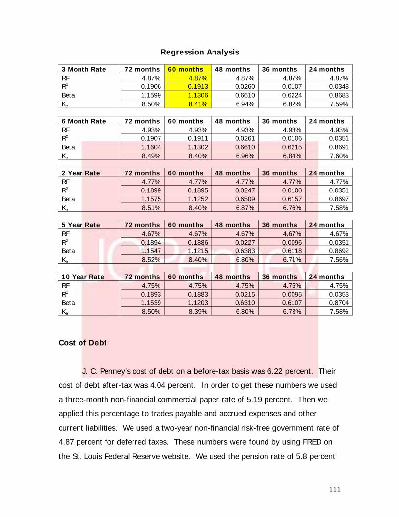
111

Regression Analysis 3 Month Rate 72 months 60 months 48 months 36 months 24 months RF 4.87% 4.87% 4.87% 4.87% 4.87%R2 0.1906 0.1913 0.0260 0.0107 0.0348Beta 1.1599 1.1306 0.6610 0.6224 0.8683Ke 8.50% 8.41% 6.94% 6.82% 7.59% 6 Month Rate 72 months 60 months 48 months 36 months 24 months RF 4.93% 4.93% 4.93% 4.93% 4.93%R2 0.1907 0.1911 0.0261 0.0106 0.0351Beta 1.1604 1.1302 0.6610 0.6215 0.8691Ke 8.49% 8.40% 6.96% 6.84% 7.60% 2 Year Rate 72 months 60 months 48 months 36 months 24 months RF 4.77% 4.77% 4.77% 4.77% 4.77%R2 0.1899 0.1895 0.0247 0.0100 0.0351Beta 1.1575 1.1252 0.6509 0.6157 0.8697Ke 8.51% 8.40% 6.87% 6.76% 7.58% 5 Year Rate 72 months 60 months 48 months 36 months 24 months RF 4.67% 4.67% 4.67% 4.67% 4.67%R2 0.1894 0.1886 0.0227 0.0096 0.0351Beta 1.1547 1.1215 0.6383 0.6118 0.8692Ke 8.52% 8.40% 6.80% 6.71% 7.56% 10 Year Rate 72 months 60 months 48 months 36 months 24 months RF 4.75% 4.75% 4.75% 4.75% 4.75%R2 0.1893 0.1883 0.0215 0.0095 0.0353Beta 1.1539 1.1203 0.6310 0.6107 0.8704Ke 8.50% 8.39% 6.80% 6.73% 7.58%

Cost of Debt

J. C. Penney’s cost of debt on a before-tax basis was 6.22 percent. Their

cost of debt after-tax was 4.04 percent. In order to get these numbers we used

a three-month non-financial commercial paper rate of 5.19 percent. Then we

applied this percentage to trades payable and accrued expenses and other

current liabilities. We used a two-year non-financial risk-free government rate of

4.87 percent for deferred taxes. These numbers were found by using FRED on

the St. Louis Federal Reserve website. We used the pension rate of 5.8 percent

112

provided in the 10-K and applied this to other liabilities. We did so because

pensions were the main expense that the company paid and characterized as

other liabilities. A corporate tax rate of 35 percent was provided within the

company’s 2006 10-K.

The interest rate for the company’s long-term debt was 7.69 percent. We

calculated this number by taking every item listed under long-term debt within

the company’s annual 10-K. Each was provided with a rate, and a weight for

each one was calculated by making each one a percentage of total long-term

debt. We then multiplied the rate by the estimated weight to get the value

ranked weight for each line item.

In order to get the cost of debt estimations we took all the liability

amounts listed in the annual 10-K and set them all as percentages of total

liabilities. We then multiplied those percentages by the interest rates we derived

in the above paragraphs. This gave us a value added weight for each line item

under total liabilities. We took the sum of all of these value added weights to

get the before tax cost of debt. By multiplying this number by 1 minus the

corporate tax rate, we derived the after tax weighted average cost of debt.

Weighted Average Cost of Capital

After getting the cost of equity and cost of debt, we plugged them into

the WACC formula with a Ke of 13.61 percent. This number was calculated using

CAPM with the provided risk-free rates located in the 10-K, the S&P 500 average

market return, and the beta we derived from our regression analysis. The before

tax weighted average cost of capital was 8.72 percent and the after tax cost of

capital was 7.28 percent (by using 1 minus the tax rate).

113

Intrinsic Valuations

Intrinsic valuations give a better overall picture of the firm as a group

compared to the comparable methods. The reason is that the four intrinsic

methods used to value J. C. Penney slice and dice the company, looking at many

different angles of valuation. The methods used were the discounted dividend

model, the free cash flows model, residual income model, and the long run ROE

residual income model. Following is a discussion of each of the models and their

relevance in valuing the J. C. Penney Company.

Discount Dividends Model

The discount dividends model values a firm by the value it holds for its

shareholders. Shareholders consider receiving value from a firm they invest in

by the dividends they receive. Therefore, this method consists of discounting the

future dividends back to present value to value the firm. This method is not very

reliable due to several factors. First, we must assume the profitability of a

company to go on for an indefinite period whereas in real life it could go

bankrupt. In addition, dividends generally increase in a stepladder fashion. This

means that dividends remain at the same level for some time and then they

“step” into a higher value for some time and so forth. This has a very small

volatility measure, therefore not showing the volatility that is within the pricing of

a firm from day to day. This just shows it’s a very inaccurate way to value a

firm. Following is the model in respect for J. C. Penney.

114

Sensitivity Analysis Growth Rates 0.105 0.11 0.114 0.115 0.1175 0.118 $25.91 $41.34 $77.77 $102.06 $587.81 0.12 $23.08 $34.05 $50.71 $63.20 $121.49

Ke 0.1361 $13.53 $16.06 $18.08 $18.71 $20.57 0.15 $11.36 $12.17 $12.98 $13.21 $13.85 0.16 $10.18 $10.71 $11.22 $11.36 $11.74 Over Valued <$69.69 Fairly Valued within 15% Under-valued >$94.24 Actual PPS (as of June 1, 2007)- $81.99

To calculate the value of J. C. Penney using this valuation model, we first

looked at our dividends. We took an average of the change in dividends, took

out some outliers, and saw a consistent increase of 11 percent about every three

years. We believe J. C. Penney will continue to increase their dividends in this

fashion due to the consistent profitability they have had the last couple of years.

We then discounted these dividends back to present value and found the sum.

Once we added up the dividends for the next ten years, we used the perpetuity

equation to value the firm for the indefinite amount of time past ten years. This

is valued by using a selected dividend amount divided by cost of equity minus

growth of dividends. We decided not to grow dividends anymore since in the

past they had kept a dividend amount for more than 3 years. Since we were so

aggressive in our growth for the next ten years, we assumed they would

maintain the dividend amount at about a dollar for a long period of time.

Therefore, we kept the 99 cents we had for the last four years. This perpetuity

came out to be $37.93 in year ten value. So we then discounted back to the

present value of $10.59. We added the value of the firm for the next ten years

with the value of the perpetuity and came up with the value of our company.

The total value of our firm as of January 2007 came out to be $15.53 per

share. Since we are valuing our firm as of June 1, 2007, we then had to grow

our share price to June 1 and the new implied share price is $16.06. This

amount is a lot smaller than the amount of J. C. Penney’s share price in the

market of $81.99. This shows that our company is overvalued by a large

115

amount in the eye’s of shareholders due to the small dividends that are paid out.

If one were to divide the present value of the sum of the dividends for the next

ten years and the perpetuity dividend present value by the total value of the

firm, one can notice that about 70 percent of the value of our firm comes from

the perpetuity. This proves how inaccurate this model can be because we are

relying heavily on a perpetuity that is full of assumptions.

Within our sensitivity analysis, we observed that the only way J. C. Penney

was fairly valued was by cutting cost of equity to 11.8 percent and having a

dividend growth rate of 11.4 percent. We believe that J. C. Penney could not cut

their cost of equity all the way to only 11.8 percent from their actual 13.61

percent at the moment. J. C. Penney could be undervalued if the cost of equity

was cut down to 12 percent or lower and needed to grow dividends at least at

11.5 percent. We do not believe J. C. Penney could cut the cost of equity that

much or grow dividends at these rates because besides some outliers it has

never followed this pattern in the past. Even though the discount model does

not show a clear understanding of our firm due to the low dividend payments, it

illustrates that J. C. Penney is overvalued due to its high share price of $81.99.

Free Cash Flows Model

The free cash flow model compares the cost of capital to growth rate on

the perpetuity. The percentage of the both present value of future cash flows

and terminal value perpetuity are almost equally weighted in the valuation of the

firm. For this reason, this model is seen as a fairly inaccurate model. Even

though cash flows make up about 58 percent of the value, 42 percent is still a

large weight to have on a number so sensitive to growth rates. Following is the

sensitivity analysis and discussion of the free cash flows model applied to the J.

C. Penney Company.

116

Sensitivity Analysis Growth Rates 0.04 0.05 0.059 0.065 0.07 0.07 $43.89 $61.24 $103.84 $217.45 n/a 0.08 $30.54 $38.44 $ 52.00 $ 70.07 $101.70 WACC 0.0872 $24.03 $29.09 $ 36.70 $ 45.21 $ 56.84

BT 0.1 $15.74 $18.38 $ 21.84 $ 25.15 $ 28.91 0.11 $10.99 $12.70 $ 14.83 $ 16.71 $ 18.72 Undervalued <$69.69 Fairly Valued Overvalued >$94.29 Actual PPS (June 1, 2007): $81.99

The free cash flows model requires the following information: forecasted

earnings, dividends, cash flows from operations and investments, the before tax

weighted average cost of capital, book value of equity, and growth rate of the

perpetuity.

To begin, the difference in operating cash flows and investing cash flows

gives the annual free cash flow. Because we are looking at year now, all of

these cash flows had to be brought back by multiplying them by the present

value factor. The sum of all of these cash flows, $9,504 million, plus the present

value of the perpetuity, $6,747 million, gave us the value of the firm,$16,251

million. This value minus the book value of liabilities leads to the market value of

equity divided by the number of shares outstanding to reach the estimated price

per share.

$16,251-8,385=$7,866

$7,866/266=$34.80

Because J. C. Penney’s fiscal year ends on January 31, this price per share

was not in fact the price used to value our sensitivity analysis. To bring this

number to June 1, 2007, the date of firm valuation, this share price was

multiplied by the weighted average cost of capital raised to five months divided

by twelve months.

$34.80*1.0872^(5/12)=$36.70

117

This particular stock price in our sensitivity analysis used a WACC of 8.72 percent

and a growth rate of 5.9 percent. From here, we can begin to draw conclusions

and form a sensitivity analysis.

The free cash flows model shows us, like many of our other models, that

the firm is overvalued at June 1, 2007. Most of our conclusions draw on the fact

the firm is overvalued. The few that fell into the firm being fairly valued, +/- 15

percent, required a weighted average cost of capital of 8 percent and growth

rates ranging from 5.9 to 6.5 percent. Once again, this model relays that J. C.

Penney is an overvalued firm.

Residual Income Model

Of all the intrinsic valuation models, this is said to be the most accurate.

This is explained by the very high percentage of the present value of residual

income in the overall value of the firm. Because this number is based off of

forecasted values of earnings rather than perpetuities, this model is a fairly

accurate glace at the firm. Following is the sensitivity analysis and discussion of

the residual income model in respect to J. C. Penney.

Sensitivity Analysis Growth Rate 0 -0.15 -0.25 -0.4 -0.5

0.05 127.8 78.08 72.55 68.87 67.53 0.07 79.18 60.3 57.55 55.62 54.98

Ke 0.09 53.73 47.22 46.07 45.22 44.9 0.11 38.62 37.45 37.21 37.02 36.95

0.1361 26.61 28.15 28.52 28.81 28.93

Undervalued <$69.69 Fairly Valued Overvalued >$94.29 Actual PPS (June 1, 2007): $81.99

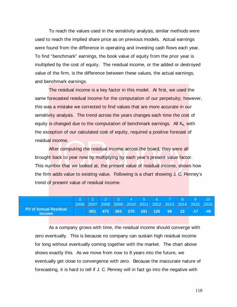
118

To reach the values used in the sensitivity analysis, similar methods were

used to reach the implied share price as on previous models. Actual earnings

were found from the difference in operating and investing cash flows each year.

To find “benchmark” earnings, the book value of equity from the prior year is

multiplied by the cost of equity. The residual income, or the added or destroyed

value of the firm, is the difference between these values, the actual earnings,

and benchmark earnings.

The residual income is a key factor in this model. At first, we used the

same forecasted residual income for the computation of our perpetuity; however,

this was a mistake we corrected to find values that are more accurate in our

sensitivity analysis. The trend across the years changes each time the cost of

equity is changed due to the computation of benchmark earnings. All Ke, with

the exception of our calculated cost of equity, required a positive forecast of

residual income.

After computing the residual income across the board, they were all

brought back to year now by multiplying by each year’s present value factor.

This number that we looked at, the present value of residual income, shows how

the firm adds value to existing value. Following is a chart showing J. C. Penney’s

trend of present value of residual income.

0 1 2 3 4 5 6 7 8 9 10 2006 2007 2008 2009 2010 2011 2012 2013 2014 2015 2016

PV of Annual Residual Income 601 473 363 270 191 125 68 22 -17 -49

As a company grows with time, the residual income should converge with

zero eventually. This is because no company can sustain high residual income

for long without eventually coming together with the market. The chart above

shows exactly this. As we move from now to 8 years into the future, we

eventually get close to convergence with zero. Because the inaccurate nature of

forecasting, it is hard to tell if J. C. Penney will in fact go into the negative with

119

residual income or converge. Future re-evaluation will be necessary to confirm

this or justify the company destroying value.

The residual income model is said to be one of the best of the four models

in explaining what is happening with the market price of stock. As we look at

the model, again we see that the firm is consistently overvalued in share price.

These figures show that the firm’s calculated cost of equity consistently shows

across the board a very low price. To get anywhere close to the price at June 1,

2007, the grow rate would either have to be ridiculously high, or the firm would

have to have an unrealistically low cost of equity. Either way, the numbers

would not make sense for the values that were calculated in this table. Once

again, the conclusion drawn from researching the residual income model is that

our firm, J. C. Penney, is overvalued.

120

Long Run Return on Equity Residual Income Model

The long run return on equity residual income model calculates the value

of the firm by using a perpetuity equation that can be derived from the methods

of the residual income model. Although it is a perpetuity, it is a very accurate

model due to the key factors that are used to value the firm within this particular

model. It links the cost of equity, long run return on equity, and long run growth

on equity. Following is the model in respect to the J. C. Penney Company.

Growth=.11 ROE 0.13 0.15 0.17 0.19 0.21 0.125 $26.68 $53.36 $80.04 $106.72 $133.40

Ke 0.13 $20.01 $40.02 $60.03 $80.04 $100.05 0.1361 $15.33 $30.67 $46.00 $61.33 $76.66 0.14 $13.34 $26.68 $40.02 $53.36 $66.70 0.145 $10.84 $22.87 $34.30 $45.74 $57.17

ROE= .13 Growth Rate 0.09 0.1 0.11 0.12 0.13 0.125 $22.87 $24.01 $26.68 $40.02 $0.00

Ke 0.13 $20.01 $20.01 $20.01 $20.01 n/a 0.1361 $17.36 $15.77 $15.33 $12.43 $0.00 0.14 $16.01 $15.01 $13.34 $10.00 $0.00 0.145 $14.55 $13.34 $11.43 $8.00 $0.00

Over Valued <$69.69 Fairly Valued within 15% of $81.99 Under-valued >$94.24 Actual PPS (as of June 1, 2007)- $81.99

Ke =.1361 Growth Rate 0.09 0.1 0.11 0.12 0.13 0.21 $52.09 $60.97 $76.66 $111.85 $262.42 0.19 $43.40 $49.89 $61.33 $87.00 $196.81

ROE 0.17 $34.72 $38.80 $46.00 $62.14 $131.21 0.15 $26.04 $27.71 $30.67 $37.28 $65.60 0.13 $17.36 $16.63 $15.33 $12.43 $0.00

121

To find our long run return on equity, we found the ROE for the next ten

years using our forecasted earnings and book value of equity. The book value of

equity had not been forecasted but it is very simple to find by using the following

equation:

Ending BVE= Beginning BVE +Earnings- Dividends

Once this was done we used the return on equity equation of:

ROE= Net Income (Earnings) of this year/ BVE of previous year

ROE 29.52% 24.97% 21.77% 19.39% 17.60% 16.17% 15.00% 14.06% 13.26% 12.57%

We got the results above that helped us see the pattern of J. C. Penney’s return

on equity for the next ten years so we could make some assumptions of the long

run return on equity. J. C. Penney’s return on equity has a trend of decreasing

until it hits a plateau at around 12 percent.

We then needed to find the long-run growth of return on equity. We

calculated the percentage change of book value of equity in order to see the long

run trend. This percentage change was calculated by taking this year’s book

value of equity divided by the previous years book value of equity then

subtracted that amount by one.

We got the results above that helped us see the decreasing growth

pattern of J. C. Penney’s book value of equity. We assumed that it has on

average hit a plateau of about 11 percent.

BVE % Growth 25.30% 21.61% 19.00% 16.80% 15.38% 14.24% 13.13% 12.40% 11.78% 11.25%

122

Once we found both long-run return on equity and long-run growth of

equity, we plugged these numbers into the following equation:

Value of Firm= BVE (1+((LR Return on Equity – Ke /( Ke - LR Growth of Equity))

We then divided by the amount of outstanding shares we have at the moment,

226, to get our individual price per share. Our price per share through this

model came out to be about $14.54 for January 2007. We then grew this

number to June 2007 in the amount of $15.33.

This amount definitely shows that J. C. Penney is overvalued. Within our

sensitivity analysis, by manipulating the numbers, J. C. Penney was, for the most

part, overvalued no matter if we increased growth of equity, return on equity, or

cut cost of equity. The only way our firm could be fairly valued would be to

grow our return on equity to about 21 percent which does not seem feasible

since the trend shows that we are decreasing to smaller percentages. Overall,

the sensitivity analysis helps confirm that our company is overvalued by this

valuation method.

Abnormal Earnings Growth Model

Abnormal earnings growth model brings theory to the price earnings ratio.

It links the capitalized forward earnings and the extra value created from

abnormal earnings growth. The main difference between this model and the

others is this one discounts back to year one instead of year zero and it keeps a

constant perpetuity. This is a very accurate model and can be proven because it

is linked directly to residual income. Following is the sensitivity analysis and

discussion of the abnormal earnings growth model in respect to J. C. Penney.

123

Sensitivity Analysis Growth Rates 0 -0.15 -0.25 -0.4 -0.5 0.05 47.35 62.29 65.8 68.61 69.75 0.07 33.82 44.49 47.00 49.01 49.82

Ke 0.09 26.31 34.61 36.56 38.12 38.75 0.11 21.52 28.31 29.91 31.19 31.70 0.1361 17.40 22.88 24.17 25.21 25.62 Undervalued <$69.69 Fairly Valued Overvalued >$94.29 Actual PPS (June 1, 2007): $81.99

We first had to calculate the cumulative dividend income by adding

forecasted earnings to our drip income. Drip income is found by multiplying the

previous year’s dividend by our cost of equity. Once the cumulative dividend

income is found, we needed to calculate the normal income, “benchmark”, by

taking the previous year’s earnings times one plus J. C. Penney’s cost of equity

which is 13.61 percent. To find the annual AEG, which links our residual income

model to our AEG model, we take the cumulative dividend income minus the

calculated benchmark. We then had to bring back these values to year one by

multiplying by the present value factor. The present value factor is calculated by

taking one divided by one plus the cost of equity to the previous time period.

Once the present values of our annual AEG components were found, we added

all of these together to get the total present value of the abnormal earnings

growth, -453.20.

We then had to find the value of the perpetuity to account for the years

out to infinity. To do this, we forecasted an abnormal earnings growth for year

eleven that followed our pattern of abnormal earnings growth. This value came

to be -131 million. We then plugged it into the perpetuity equation:

AEG Perpetuity = forecasted AEG/(JCP Ke - growth)

124

This value of the perpetuity then needed to be brought back to year one from

year ten. We did this by multiplying by the present value factor of year ten. We

then summed the core earnings, which are the forecasted earnings in 2007, plus

the perpetuity present value and the sum of the present value of abnormal

earnings growth. To find our value of equity, we took this sum and divided by

the J. C. Penney’s cost of equity. Finally, we took our number of shares

outstanding at present time and divided it into our value of equity to come up

with our estimated price per share of $22.88 adjusted to June 1, 2007.

During our sensitivity analysis, we used aggressive negative growth rates

to attempt to reach our current share price. We were only successful in reaching

a fairly valued share price by cutting cost of equity to .05 and having a growth

rate of -50 percent. This proves along with our other models that J. C. Penney is

extremely overvalued since we couldn’t achieve a fairly valued price because we

do not believe J. C. Penney could cut cost of equity to .05 and growth of -50

percent is not achievable.

Abnormal Earnings Growth and Residual Income Proof

As mentioned previously, the abnormal earnings growth and residual

income models are linked. If one were to take the change in residual income

from 2008 to 2007, the result would be the annual abnormal earnings growth

from 2008. The chart above illustrates this for our forecasted years up to 2016.

This can help verify that the valuation models are correctly calculated.

Because of this link, the abnormal earnings growth and residual income

valuation share price should be very close. Our models came up with prices that

were about nine dollars apart. After reviewing our numbers, we looked carefully

at the perpetuity and realized that was where our numbers differed. The reason

2008 2009 2010 2011 2012 2013 2014 2015 2016Annual AEG -71.72 -77.50 -83.63 -87.29 -94.18 -101.47 -106.12 -114.32 -123.01Change in RI -71.72 -77.50 -83.63 -87.29 -94.18 -101.47 -106.12 -114.32 -123.01

125

for this large difference between share prices is that our residual income

perpetuity had no variation after 2011. Tying this back to what was mentioned

above, the change in residual income should equal the annual abnormal earnings

growth. Since our residual income is a fixed number, the abnormal earnings

growth after 2011 would be zero if we followed that rule. This is a limitation

because of the nature of the perpetuity and it is not likely that our abnormal

earnings growth would become zero.

This large difference between the two valuation share prices will become

smaller as the perpetuity goes on to infinity. We set up our sensitivity analysis

cost of equity and growth rates the same to be able to compare. We used

aggressive growth rates all the way up to -50 percent to attempt to reach a small

difference between the two prices. We were able to close the gap to about three

dollars. Overall, this proves that the share price valuations are closely related

besides limitations within the perpetuities.

Conclusion

After looking at all theoretical valuation models, we believe that J. C.

Penney is overvalued at its June 1, 2007 share price of $81.99. Even though the

dividend model shows the company as overvalued, we have determined that this

particular model is irrelevant in the case of our company due to the fact that the

share price moved as low at $10.18 and as high as $587.81. The drastic

fluctuations in share price were a definite indicator that the model is not useful in

our case. The J. C. Penney Company, according to all of the sensitivity analysis’

conclusions, is overvalued anywhere from $40.00-$55.00 at June 1, 2007.

126

Credit Analysis

We evaluated J. C. Penney’s credit worthiness using the Altman Z-score

model, which weights five variables to compute a bankruptcy score (Palepu).

The Altman Z-score predicts bankruptcy when the score is lower than 1.81.

Firms with a score between 1.81 and 2.67 are considered to be borderline.

Firms are considered to be healthy and to have a low risk of bankruptcy if they

score above a 3. “This is a relatively accurate model -- real world application of

the Z-Score successfully predicted 72 percent of corporate bankruptcies two

years prior to these companies filing for Chapter 7” (www.investopedia.com).

The only problem with this model is that it favors mature companies or

established companies over new start up companies because new start ups do

not possess a financial history upon which to base a score.

The Altman Z-score is calculated using the following formula:

Z-Score = 1.2(Working Capital/Total Assets) + 1.4(Retained Earnings/Total

Assets) + 3.3(Earnings before Interest and Taxes/Total Assets) + .6(Market

Value of Equity/Book Value of Debt) + 1.0(Sales/Total Assets)

Altman Z-score

2002 2003 2004 2005 2006

Z-score 2.75 1.91 3.04 3.43 3.80

According to the Altman Z-score model, J. C. Penney’s current Z-score is

3.80; however, in 2003, J. C. Penney was borderline bankruptcy according to the

model. This was caused by the discontinuation of operations of its subsidiaries,

Eckerd Pharmacy and Rojas Renner S.A. Since the sale of Eckerd Pharmacy and

Rojas Renner S.A., J. C. Penney’s score has steadily risen from 3.04 to 3.80.

127

Analyst Recommendation

After careful consideration and research of the J.C. Penny Company,

including an industry analysis, accounting analysis, financial analysis, forecasting

and future financial statements, and valuation model conclusions, we consider

the firm to be highly overvalued and should be set to sell.

Assumptions used to calculate all relevant information were taken

considering past financials of the company as well as four other competitors,

Stein Mart, Kohl’s, Dillard’s, and Stage Stores, Inc. This department retail

industry is very highly concentrated with relevant competition set as those who

take advantage of similar key success factors such as economies of scale and

scope, supplier relationships, and brand creation within different stores.

Looking at accounting ratios, J. C. Penney held the standard of the

industry and even surpassed many competitors in respect to sales being

supported by business happenings. There were no problems found or any

indication that financial statements have been manipulated to reflect better

numbers in the last five years of the business. Appropriate values were reflected

in the years where J. C. Penney sold unprofitable assets, and again reveal the

turnaround after the fact. If anything, disclosure has only improved year by

year, making the company fairly easy to value. As for financial ratios, we

deemed that J.C. Penney overall had a superior performance over the market.

When forecasting the financial statements of the company, not only were

trends of the past five years of the company used, but also that of the

competitors. We feel the growth percentage used was fairly chosen, if not a

little conservative in estimation, and gives an accurate look into the future.

Even though no real problems were found and the company seems to fly

above the competition on many aspects, the valuation models used based off of

these future forecasts show that the company is overvalued. Even after deeming

128

the discount dividend model irrelevant to our company, all other models

consistently showed an overall picture of overvaluations.

After consideration of all aspects, we recommend that the stock of J. C.

Penney be set to sell. Throughout this analysis, company stock prices were

compared to the price at June 1, 2007, $81.99. We feel that our valuations are

correct seeing that the price on June 22, 2007 is at $72.98. The market has

obviously realized what we have found, that the company is overvalued. We

also see an opportunity to buy put options on the stock. If we are on target,

buying at put option for next month would give the market a little more time to

continue to realize this, giving investors the chance to cash in on the

overvaluation.

129

Appendix

Liquidity Ratios Current ratio Inventory Turnover

2002 2003 2004 2005 2006 2002 2003 2004 2005 2006

JCP 2.008 1.735 2.445 2.427 1.904 JCP 4.565 3.538 3.561 3.553 3.552

KSS 2.178 2.695 2.502 2.443 1.773 KSS 3.676 4.286 3.897 3.861 3.822

DDS 3.531 2.263 2.194 1.874 2.096 DDS 3.296 3.167 2.895 2.781 2.840

SSI 3.610 2.737 2.572 2.434 2.578 SSI 3.392 2.667 3.140 3.358 3.296

SMRT 1.855 2.553 2.190 2.386 2.033 SMRT 6.215 8.473 6.032 6.116 6.411

Quick asset ratio Days supply of inventory

2002 2003 2004 2005 2006 2002 2003 2004 2005 2006

JCP 0.764 0.860 1.477 1.190 0.862 JCP 79.959 103.165 102.498 102.731 102.749

KSS 1.032 1.156 1.096 1.110 n/a KSS 99.286 85.167 93.666 94.535 95.511

DDS 1.670 1.012 0.486 0.272 0.209 DDS 110.755 115.241 126.064 131.229 128.535

SSI 0.199 0.111 0.283 0.217 0.099 SSI 107.594 136.854 116.228 108.680 110.750

SMRT 0.087 0.135 0.555 0.782 0.228 SMRT 58.732 43.080 60.507 59.679 56.937

Accounts receivable turnover Working capital turnover

2002 2003 2004 2005 2006 2002 2003 2004 2005 2006

JCP 45.882 76.335 45.604 69.559 75.677 JCP 7.713 6.447 3.700 4.767 6.306

KSS 9.205 8.940 8.420 8.112 n/a KSS 5.135 5.405 5.349 5.319 10.486

DDS 5.912 6.378 780.082 603.704 726.690 DDS 3.526 4.503 6.031 7.537 7.132

SSI 79.430 27.689 n/a n/a n/a SSI 3.201 4.217 5.524 6.041 6.111

SMRT 286.369 320.666 249.420 133.227 147.707 SMRT 9.662 7.286 6.910 6.135 8.589

Days sales outstanding 2002 2003 2004 2005 2006 JCP 7.955 4.782 8.004 5.247 4.823 KSS 39.653 40.829 43.349 44.993 n/a DDS 61.737 57.231 0.468 0.605 0.502 SSI 4.595 13.182 n/a n/a n/a SMRT 1.275 1.138 1.463 2.740 2.471

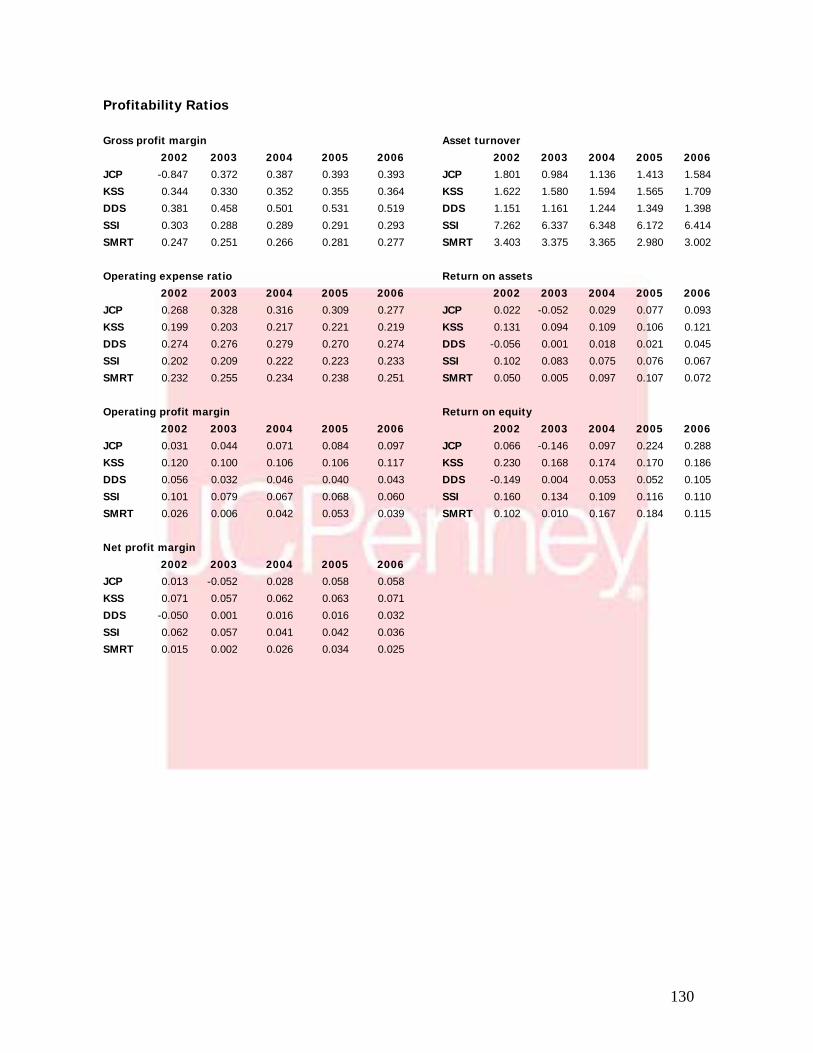
130

Profitability Ratios Gross profit margin Asset turnover

2002 2003 2004 2005 2006 2002 2003 2004 2005 2006

JCP -0.847 0.372 0.387 0.393 0.393 JCP 1.801 0.984 1.136 1.413 1.584

KSS 0.344 0.330 0.352 0.355 0.364 KSS 1.622 1.580 1.594 1.565 1.709

DDS 0.381 0.458 0.501 0.531 0.519 DDS 1.151 1.161 1.244 1.349 1.398

SSI 0.303 0.288 0.289 0.291 0.293 SSI 7.262 6.337 6.348 6.172 6.414

SMRT 0.247 0.251 0.266 0.281 0.277 SMRT 3.403 3.375 3.365 2.980 3.002

Operating expense ratio Return on assets

2002 2003 2004 2005 2006 2002 2003 2004 2005 2006

JCP 0.268 0.328 0.316 0.309 0.277 JCP 0.022 -0.052 0.029 0.077 0.093

KSS 0.199 0.203 0.217 0.221 0.219 KSS 0.131 0.094 0.109 0.106 0.121

DDS 0.274 0.276 0.279 0.270 0.274 DDS -0.056 0.001 0.018 0.021 0.045

SSI 0.202 0.209 0.222 0.223 0.233 SSI 0.102 0.083 0.075 0.076 0.067

SMRT 0.232 0.255 0.234 0.238 0.251 SMRT 0.050 0.005 0.097 0.107 0.072

Operating profit margin Return on equity

2002 2003 2004 2005 2006 2002 2003 2004 2005 2006

JCP 0.031 0.044 0.071 0.084 0.097 JCP 0.066 -0.146 0.097 0.224 0.288

KSS 0.120 0.100 0.106 0.106 0.117 KSS 0.230 0.168 0.174 0.170 0.186

DDS 0.056 0.032 0.046 0.040 0.043 DDS -0.149 0.004 0.053 0.052 0.105

SSI 0.101 0.079 0.067 0.068 0.060 SSI 0.160 0.134 0.109 0.116 0.110

SMRT 0.026 0.006 0.042 0.053 0.039 SMRT 0.102 0.010 0.167 0.184 0.115

Net profit margin 2002 2003 2004 2005 2006 JCP 0.013 -0.052 0.028 0.058 0.058 KSS 0.071 0.057 0.062 0.063 0.071 DDS -0.050 0.001 0.016 0.016 0.032 SSI 0.062 0.057 0.041 0.042 0.036 SMRT 0.015 0.002 0.026 0.034 0.025

131

Capital Structure Ratio

Debt to equity ratio

2002 2003 2004 2005 2006

JCP 1.805 2.373 1.909 2.110 1.955

KSS 0.798 0.607 0.607 0.537 0.614

DDS 4.070 3.747 2.705 2.516 1.947

SSI 0.293 0.394 0.427 0.458 0.444

SMRT 0.837 0.726 0.716 0.606 0.667

Times interest earned

2002 2003 2004 2005 2006

JCP 15.961 -10.866 -4.893 -16.467 14.785

KSS 18.341 13.601 19.279 19.646 27.191

DDS 2.687 1.506 2.820 3.027 3.145

SSI -49.590 -31.428 -33.051 -30.990 -18.518

SMRT 13.815 4.700 1567.923 undefined undefined

Debt service margin

2002 2003 2004 2005 2006

JCP 0.506 0.421 0.521 0.720 0.712

KSS 40.784 2.122 75.637 254.530 28.714

DDS 3.631 3.113 3.337 4.029 1.817

SSI 533.599 1487.495 347.491 815.438 745.473

SMRT 0.722 undefined undefined undefined undefined

132

Method of Comparables PPS EPS forecast EPS DPS BPS BV EV FCF

JCP 81.99 11.3 5.03 0.72 18.99 18.99 19.29 -

269.00 KSS 70.27 4.51 3.49 N/A 18.32 25.2 DDS 34.62 1.84 2.81 0.16 32.76 3.95 SSI 21.02 1.66 1.25 0.12 13.19 0.92 SMRT 12.57 0.96 0.86 1.75 6.761 0.54 Industry AVG

P/E

(trailing) P/E

(forward) P/B D/P P.E.G EBITDA P/EBITDA P/FCF EV/EBITDA

(in

billions) JCP 16.30 7.26 4.32 0.009 2.72 2.311 3.55 N/A 8.34 KSS 20.13 15.58 3.84 N/A 0.93 2.320 3.03 84.82 10.86 DDS 12.32 18.82 1.06 0.005 3.1 0.625 5.54 N/A 6.32 SSI 16.82 12.66 1.59 0.006 0.84 0.145 14.53 N/A 6.36 SMRT 14.62 13.09 1.86 0.139 0.78 0.090 14.02 N/A 6.02 Industry AVG 15.97 15.04 2.09 0.05 1.413 0.795 9.47 84.82 7.390

Price Comparables Trailing Forward P/E 80.34 75.64 P/B 39.62 D/P 14.44 PEG 42.55 P/EBITDA 21.90 EV/EBITDA 72.17 P/FCF N/A

133

3 Month Regression SUMMARY OUTPUT 72 Months

Regression Statistics Multiple R 0.449493363 R Square 0.202044283 Adjusted R Square 0.190644916 Standard Error 0.085209953 Observations 72 ANOVA

df SS MS F Significance F Regression 1 0.128690494 0.128690494 17.72416631 7.46639E-05 Residual 70 0.508251528 0.007260736 Total 71 0.636942022

Coefficients Standard Error t Stat P-value Lower 95% Upper 95% Lower 95.0% Upper 95.0% Intercept 0.02395843 0.01004484 2.385148001 0.019783542 0.003924629 0.043992231 0.003924629 0.043992231 X Variable 1 1.159873034 0.275503768 4.210007875 7.46639E-05 0.610398101 1.709347967 0.610398101 1.709347967 SUMMARY OUTPUT 60 months

Regression Statistics Multiple R 0.452814378 R Square 0.205040861 Adjusted R Square 0.191334669 Standard Error 0.077782436 Observations 60 ANOVA

df SS MS F Significance F Regression 1 0.090507942 0.090507942 14.95972481 0.000280412 Residual 58 0.350906229 0.006050107 Total 59 0.441414171

Coefficients Standard Error t Stat P-value Lower 95% Upper 95% Lower 95.0% Upper 95.0% Intercept 0.022531053 0.010099422 2.230925039 0.029567509 0.002314864 0.042747242 0.002314864 0.042747242 X Variable 1 1.13064286 0.292323441 3.867780346 0.000280412 0.545493922 1.715791798 0.545493922 1.715791798 SUMMARY OUTPUT 48 months

Regression Statistics Multiple R 0.216255217 R Square 0.046766319 Adjusted R Square 0.026043848 Standard Error 0.065958576 Observations 48 ANOVA

df SS MS F Significance F Regression 1 0.009818252 0.009818252 2.256792556 0.139863647 Residual 46 0.200124552 0.004350534 Total 47 0.209942804

Coefficients Standard Error t Stat P-value Lower 95% Upper 95% Lower 95.0% Upper 95.0% Intercept 0.030542564 0.01011469 3.019624271 0.004120452 0.010182749 0.050902379 0.010182749 0.050902379 X Variable 1 0.660952169 0.439971162 1.502262479 0.139863647 -0.224663833 1.546568172 -0.224663833 1.546568172 SUMMARY OUTPUT 36 months

Regression Statistics Multiple R 0.197449946 R Square 0.038986481 Adjusted R Square 0.010721378 Standard Error 0.063995173 Observations 36 ANOVA

df SS MS F Significance F Regression 1 0.005648822 0.005648822 1.379315 0.248378338 Residual 34 0.139242994 0.004095382 Total 35 0.144891816

Coefficients Standard Error t Stat P-value Lower 95% Upper 95% Lower 95.0% Upper 95.0% Intercept 0.023414247 0.011021408 2.124433335 0.040986238 0.001016051 0.045812443 0.001016051 0.045812443 X Variable 1 0.622418625 0.529969468 1.174442421 0.248378338 -0.454608911 1.699446162 -0.454608911 1.699446162

134

3 Month Regression SUMMARY OUTPUT 24 Months

Regression Statistics Multiple R 0.277145786 R Square 0.076809786 Adjusted R Square 0.034846595 Standard Error 0.058490786 Observations 24 ANOVA

df SS MS F Significance F Regression 1 0.006262143 0.006262143 1.830408596 0.189820587 Residual 22 0.075265784 0.003421172 Total 23 0.081527927

Coefficients Standard Error t Stat P-value Lower 95% Upper 95% Lower 95.0% Upper 95.0% Intercept 0.018089978 0.012709597 1.423332134 0.168667626 -0.008268113 0.044448068 -0.008268113 0.044448068 X Variable 1 0.86829239 0.64178856 1.352925939 0.189820587 -0.462695614 2.199280393 -0.462695614 2.199280393

135

6 Month Regression SUMMARY OUTPUT 72 Month

Regression Statistics Multiple R 0.44952832 R Square 0.20207571 Adjusted R Square 0.190676792 Standard Error 0.085208275 Observations 72 ANOVA

df SS MS F Significance F Regression 1 0.128710511 0.128710511 17.72762139 7.45559E-05 Residual 70 0.508231511 0.00726045 Total 71 0.636942022

Coefficients Standard Error t Stat P-value Lower 95% Upper 95% Lower 95.0% Upper 95.0% Intercept 0.024086144 0.010043978 2.398068263 0.019151538 0.004054063 0.044118226 0.004054063 0.044118226 X Variable 1 1.160350997 0.275590438 4.210418197 7.45559E-05 0.610703206 1.709998788 0.610703206 1.709998788 SUMMARY OUTPUT 60 Month

Regression Statistics Multiple R 0.452575365 R Square 0.204824461 Adjusted R Square 0.191114538 Standard Error 0.077793022 Observations 60 ANOVA

df SS MS F Significance F Regression 1 0.09041242 0.09041242 14.93986943 0.000282764 Residual 58 0.351001752 0.006051754 Total 59 0.441414171

Coefficients Standard Error t Stat P-value Lower 95% Upper 95% Lower 95.0% Upper 95.0% Intercept 0.022669716 0.010097087 2.24517387 0.028584318 0.002458201 0.042881232 0.002458201 0.042881232 X Variable 1 1.130202094 0.292403594 3.865212728 0.000282764 0.544892712 1.715511476 0.544892712 1.715511476 SUMMARY OUTPUT 48 Month

Regression Statistics Multiple R 0.216486835 R Square 0.04686655 Adjusted R Square 0.026146257 Standard Error 0.065955108 Observations 48 ANOVA

df SS MS F Significance F Regression 1 0.009839295 0.009839295 2.261867207 0.139429522 Residual 46 0.200103509 0.004350076 Total 47 0.209942804

Coefficients Standard Error t Stat P-value Lower 95% Upper 95% Lower 95.0% Upper 95.0% Intercept 0.030639424 0.010091375 3.036199165 0.003936725 0.01032654 0.050952308 0.01032654 0.050952308 X Variable 1 0.66096566 0.439486303 1.503950533 0.139429522 -0.223674372 1.545605692 -0.223674372 1.545605692 SUMMARY OUTPUT 36 Month

Regression Statistics Multiple R 0.197246312 R Square 0.038906107 Adjusted R Square 0.01063864 Standard Error 0.063997849 Observations 36 ANOVA

df SS MS F Significance F Regression 1 0.005637177 0.005637177 1.376356322 0.248876419 Residual 34 0.139254639 0.004095725 Total 35 0.144891816

Coefficients Standard Error t Stat P-value Lower 95% Upper 95% Lower 95.0% Upper 95.0% Intercept 0.023524249 0.010999319 2.138700426 0.03972785 0.001170943 0.045877555 0.001170943 0.045877555 X Variable 1 0.621523842 0.529776088 1.173182135 0.248876419 -0.455110698 1.698158383 -0.455110698 1.698158383

136

6 Month Regression SUMMARY OUTPUT 24 Month

Regression Statistics Multiple R 0.277563315 R Square 0.077041394 Adjusted R Square 0.03508873 Standard Error 0.058483448 Observations 24 ANOVA

df SS MS F Significance F Regression 1 0.006281025 0.006281025 1.836388596 0.189126727 Residual 22 0.075246902 0.003420314 Total 23 0.081527927

Coefficients Standard Error t Stat P-value Lower 95% Upper 95% Lower 95.0% Upper 95.0% Intercept 0.018203442 0.012677335 1.435904478 0.165096959 -0.008087741 0.044494626 -0.008087741 0.044494626 X Variable 1 0.869137911 0.641366689 1.355134162 0.189126727 -0.460975187 2.199251009 -0.460975187 2.199251009

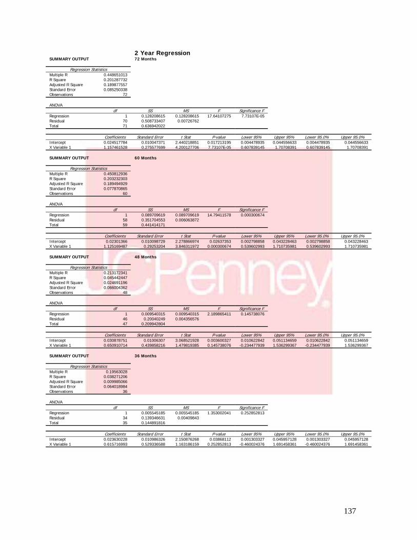
137

2 Year Regression SUMMARY OUTPUT 72 Months

Regression Statistics Multiple R 0.448651013 R Square 0.201287732 Adjusted R Square 0.189877557 Standard Error 0.085250338 Observations 72 ANOVA

df SS MS F Significance F Regression 1 0.128208615 0.128208615 17.64107275 7.73107E-05 Residual 70 0.508733407 0.00726762 Total 71 0.636942022

Coefficients Standard Error t Stat P-value Lower 95% Upper 95% Lower 95.0% Upper 95.0% Intercept 0.024517784 0.010047371 2.440218851 0.017213195 0.004478935 0.044556633 0.004478935 0.044556633 X Variable 1 1.157461528 0.275577699 4.200127706 7.73107E-05 0.607839145 1.70708391 0.607839145 1.70708391 SUMMARY OUTPUT 60 Months

Regression Statistics Multiple R 0.450812936 R Square 0.203232303 Adjusted R Square 0.189494929 Standard Error 0.077870865 Observations 60 ANOVA

df SS MS F Significance F Regression 1 0.089709619 0.089709619 14.79411578 0.000300674 Residual 58 0.351704553 0.006063872 Total 59 0.441414171

Coefficients Standard Error t Stat P-value Lower 95% Upper 95% Lower 95.0% Upper 95.0% Intercept 0.02301366 0.010098729 2.278866974 0.02637353 0.002798858 0.043228463 0.002798858 0.043228463 X Variable 1 1.125169487 0.29253204 3.846311972 0.000300674 0.539602993 1.710735981 0.539602993 1.710735981 SUMMARY OUTPUT 48 Months

Regression Statistics Multiple R 0.213172341 R Square 0.045442447 Adjusted R Square 0.024691196 Standard Error 0.066004362 Observations 48 ANOVA

df SS MS F Significance F Regression 1 0.009540315 0.009540315 2.189865411 0.145738076 Residual 46 0.20040249 0.004356576 Total 47 0.209942804

Coefficients Standard Error t Stat P-value Lower 95% Upper 95% Lower 95.0% Upper 95.0% Intercept 0.030878751 0.01006307 3.068521928 0.003600327 0.010622842 0.051134659 0.010622842 0.051134659 X Variable 1 0.650910714 0.439858216 1.479819385 0.145738076 -0.234477939 1.536299367 -0.234477939 1.536299367 SUMMARY OUTPUT 36 Months

Regression Statistics Multiple R 0.19563028 R Square 0.038271206 Adjusted R Square 0.009985066 Standard Error 0.064018984 Observations 36 ANOVA

df SS MS F Significance F Regression 1 0.005545185 0.005545185 1.353002041 0.252852813 Residual 34 0.139346631 0.00409843 Total 35 0.144891816

Coefficients Standard Error t Stat P-value Lower 95% Upper 95% Lower 95.0% Upper 95.0% Intercept 0.023630228 0.010986326 2.150876268 0.03868112 0.001303327 0.045957128 0.001303327 0.045957128 X Variable 1 0.615716993 0.529336588 1.163186159 0.252852813 -0.460024376 1.691458361 -0.460024376 1.691458361

138

2 Year Regression SUMMARY OUTPUT 24 Months

Regression Statistics Multiple R 0.27764037 R Square 0.077084175 Adjusted R Square 0.035133456 Standard Error 0.058482093 Observations 24 ANOVA

df SS MS F Significance F Regression 1 0.006284513 0.006284513 1.837493524 0.188998865 Residual 22 0.075243414 0.003420155 Total 23 0.081527927

Coefficients Standard Error t Stat P-value Lower 95% Upper 95% Lower 95.0% Upper 95.0% Intercept 0.018129626 0.012695068 1.428084255 0.167310758 -0.008198333 0.044457585 -0.008198333 0.044457585 X Variable 1 0.869702617 0.641590417 1.355541782 0.188998865 -0.460874463 2.200279697 -0.460874463 2.200279697

139

5 Year Regression SUMMARY OUTPUT 72 Months

Regression Statistics Multiple R 0.448165023 R Square 0.200851888 Adjusted R Square 0.189435486 Standard Error 0.085273595 Observations 72 ANOVA

df SS MS F Significance F Regression 1 0.127931008 0.127931008 17.59327456 7.8877E-05 Residual 70 0.509011015 0.007271586 Total 71 0.636942022

Coefficients Standard Error t Stat P-value Lower 95% Upper 95% Lower 95.0% Upper 95.0% Intercept 0.025192121 0.010049758 2.506739098 0.014510075 0.005148511 0.045235731 0.005148511 0.045235731 X Variable 1 1.154714986 0.275296989 4.19443376 7.8877E-05 0.605652461 1.703777511 0.605652461 1.703777511 SUMMARY OUTPUT 60 months

Regression Statistics Multiple R 0.449792209 R Square 0.202313032 Adjusted R Square 0.188559808 Standard Error 0.077915774 Observations 60 ANOVA

df SS MS F Significance F Regression 1 0.089303839 0.089303839 14.71022631 0.000311514 Residual 58 0.352110332 0.006070868 Total 59 0.441414171

Coefficients Standard Error t Stat P-value Lower 95% Upper 95% Lower 95.0% Upper 95.0% Intercept 0.02360573 0.010091237 2.339230592 0.022789282 0.003405925 0.043805536 0.003405925 0.043805536 X Variable 1 1.121509085 0.292410605 3.835391285 0.000311514 0.53618567 1.7068325 0.53618567 1.7068325 SUMMARY OUTPUT 48 months

Regression Statistics Multiple R 0.208538553 R Square 0.043488328 Adjusted R Square 0.022694596 Standard Error 0.066071888 Observations 48 ANOVA

df SS MS F Significance F Regression 1 0.009130062 0.009130062 2.091415241 0.154908451 Residual 46 0.200812743 0.004365494 Total 47 0.209942804

Coefficients Standard Error t Stat P-value Lower 95% Upper 95% Lower 95.0% Upper 95.0% Intercept 0.031228196 0.010020047 3.116571909 0.003149794 0.011058888 0.051397503 0.011058888 0.051397503 X Variable 1 0.638269622 0.441350925 1.446172618 0.154908451 -0.250123698 1.526662942 -0.250123698 1.526662942 SUMMARY OUTPUT 36 months

Regression Statistics Multiple R 0.194625353 R Square 0.037879028 Adjusted R Square 0.009581352 Standard Error 0.064032036 Observations 36 ANOVA

df SS MS F Significance F Regression 1 0.005488361 0.005488361 1.338591493 0.255346729 Residual 34 0.139403455 0.004100102 Total 35 0.144891816

Coefficients Standard Error t Stat P-value Lower 95% Upper 95% Lower 95.0% Upper 95.0% Intercept 0.023748778 0.01096771 2.16533597 0.037469898 0.001459709 0.046037847 0.001459709 0.046037847 X Variable 1 0.611820612 0.528810505 1.156975148 0.255346729 -0.462851627 1.686492851 -0.462851627 1.686492851

140

5 Year Regression SUMMARY OUTPUT 24 Months

Regression Statistics Multiple R 0.277607569 R Square 0.077065962 Adjusted R Square 0.035114415 Standard Error 0.05848267 Observations 24 ANOVA

df SS MS F Significance F Regression 1 0.006283028 0.006283028 1.837023129 0.189053286 Residual 22 0.075244899 0.003420223 Total 23 0.081527927

Coefficients Standard Error t Stat P-value Lower 95% Upper 95% Lower 95.0% Upper 95.0% Intercept 0.018104966 0.012701569 1.425411748 0.168072753 -0.008236476 0.044446409 -0.008236476 0.044446409 X Variable 1 0.869241061 0.641332016 1.355368263 0.189053286 -0.460800129 2.199282251 -0.460800129 2.199282251

141

10 Year Regression SUMMARY OUTPUT 72 Months

Regression Statistics Multiple R 0.44802338 R Square 0.200724949 Adjusted R Square 0.189306734 Standard Error 0.085280367 Observations 72 ANOVA

df SS MS F Significance F Regression 1 0.127850155 0.127850155 17.57936319 7.9339E-05 Residual 70 0.509091867 0.007272741 Total 71 0.636942022

Coefficients Standard Error t Stat P-value Lower 95% Upper 95% Lower 95.0% Upper 95.0% Intercept 0.025726439 0.010052102 2.55930935 0.012651148 0.005678154 0.045774724 0.005678154 0.045774724 X Variable 1 1.153914941 0.27521508 4.192775117 7.9339E-05 0.605015778 1.702814104 0.605015778 1.702814104 SUMMARY OUTPUT 60 months

Regression Statistics Multiple R 0.449504103 R Square 0.202053939 Adjusted R Square 0.188296248 Standard Error 0.077928426 Observations 60 ANOVA

df SS MS F Significance F Regression 1 0.089189472 0.089189472 14.68661734 0.000314637 Residual 58 0.352224699 0.00607284 Total 59 0.441414171

Coefficients Standard Error t Stat P-value Lower 95% Upper 95% Lower 95.0% Upper 95.0% Intercept 0.024121653 0.010083032 2.392301596 0.020003754 0.003938272 0.044305033 0.003938272 0.044305033 X Variable 1 1.120279782 0.292324765 3.832312271 0.000314637 0.535128195 1.705431369 0.535128195 1.705431369 SUMMARY OUTPUT 48 months

Regression Statistics Multiple R 0.205765882 R Square 0.042339598 Adjusted R Square 0.021520894 Standard Error 0.066111551 Observations 48 ANOVA

df SS MS F Significance F Regression 1 0.008888894 0.008888894 2.033728779 0.160594408 Residual 46 0.20105391 0.004370737 Total 47 0.209942804

Coefficients Standard Error t Stat P-value Lower 95% Upper 95% Lower 95.0% Upper 95.0% Intercept 0.031512992 0.00997864 3.158044888 0.002804139 0.011427032 0.051598951 0.011427032 0.051598951 X Variable 1 0.63097627 0.442452353 1.42608863 0.160594408 -0.25963411 1.52158665 -0.25963411 1.52158665 SUMMARY OUTPUT 36 months

Regression Statistics Multiple R 0.194433563 R Square 0.03780441 Adjusted R Square 0.00950454 Standard Error 0.064034519 Observations 36 ANOVA

df SS MS F Significance F Regression 1 0.00547755 0.00547755 1.335851016 0.25582454 Residual 34 0.139414266 0.00410042 Total 35 0.144891816

Coefficients Standard Error t Stat P-value Lower 95% Upper 95% Lower 95.0% Upper 95.0% Intercept 0.023881239 0.010942822 2.182365759 0.036086711 0.00164275 0.046119729 0.00164275 0.046119729 X Variable 1 0.610727981 0.528407296 1.155790213 0.25582454 -0.463124839 1.684580801 -0.463124839 1.684580801

142

10 Year Regression SUMMARY OUTPUT 24 Months

Regression Statistics Multiple R 0.277979006 R Square 0.077272328 Adjusted R Square 0.035330161 Standard Error 0.058476131 Observations 24 ANOVA

df SS MS F Significance F Regression 1 0.006299853 0.006299853 1.84235421 0.188437649 Residual 22 0.075228074 0.003419458 Total 23 0.081527927

Coefficients Standard Error t Stat P-value Lower 95% Upper 95% Lower 95.0% Upper 95.0% Intercept 0.018154767 0.012685701 1.43112056 0.166448405 -0.008153766 0.0444633 -0.008153766 0.0444633 X Variable 1 0.87036741 0.641233282 1.357333493 0.188437649 -0.459469018 2.200203838 -0.459469018 2.200203838

143

Cost of Equity 0.1361 Estimated Price (Jan 2007) 3285.82 Estimated Price per Share (Jan 2007) $ 14.54 Implied Share Price at June 1, 2007 15.33 Observed Share Price $81.99 $94.29 $69.69 AT WACC 0.0799 Kd 0.0332 Ke 0.1361 0 1 2 3 4 5 6 7 8 9 10 11 2006 2007 2008 2009 2010 2011 2012 2013 2014 2015 2016 2017 Earnings 1266 1342 1422 1508 1598 1694 1796 1903 2018 2139 Dividends 181 181 181 202 202 202 224 224 224 224 247.82 Book Value Equity 4288 5373 6534 7775 9082 10478 11970 13542 15221 17014 18928 ROE 29.52% 24.97% 21.77% 19.39% 17.60% 16.17% 15.00% 14.06% 13.26% 12.57% BE % G 25.30% 21.61% 19.00% 16.80% 15.38% 14.24% 13.13% 12.40% 11.78% 11.25%

ROE G 0.13 0.15 0.17 0.19 0.21 0.09 0.1 0.11 0.12 0.13 0.125 26.68 53.36 80.04 106.72 133.4 0.145 14.55 13.34 11.43 8 0 KE 0.13 20.01 40.02 60.03 80.04 100.05 KE 0.14 16.01 15.01 13.34 10 0 0.1361 15.33 30.67 46 61.33 76.66 0.1361 17.36 15.77 15.33 12.43 0 0.14 13.34 26.68 40.02 53.36 66.7 0.13 20.01 20.01 20.01 20.01 n/a 0.145 10.84 22.87 34.3 45.74 57.17 0.125 22.87 24.01 26.68 40.02 0 G 0.09 0.1 0.11 0.12 0.13 ROE 0.21 52.09 60.97 76.66 111.85 262.42 0.19 43.4 49.89 61.33 87 196.81 0.17 34.72 38.8 46 62.14 131.21 0.15 26.04 27.71 30.67 37.28 65.6 0.13 17.36 16.63 15.33 12.43 0

144

Weighted Average Cost of Debt and WACC Value Added Liabilities 2006 % of TL Interest Rate Weight Current liabilities Trade payables 1366 0.16291 5.19 0.845503 Accrued expenses and other current liabilities 1692 0.201789 5.19 1.047284 Current maturities of long-term debt 434 0.051759 7.691094 0.398084 Income taxes payable 0 0 35 0Total current liabilities 3492 0.416458 Long-term debt 3010 0.358974 7.691094 2.760906Deferred taxes 1206 0.143828 4.87 0.700444Other liabilites 677 0.080739 5.8 0.468289Long-term liabilities 4893 0.583542 Total Liabilities 8385 1 Weighted Average Cost of Debt Before Taxes: 6.220509 Ke 13.61% Weighted Average Cost of Debt After Taxes: 4.043331 WACC= (Ve/Vf)*ke + (Vd/Vf)*kd(1-t) Tax rate used: 35% Corporate Tax Rate

WACC= (4288/12673)*13.61 + (8385/12673)*6.22(1-.35)

AT WACC 7.280 BT WACC 8.720 ** Used 17 year S&P 500 average market return

145

Discount Dividends Model 0 1 2 3 4 5 6 7 8 9 10 11 2006 2007 2008 2009 2010 2011 2012 2013 2014 2015 2016 2017

Earnings $ 1,266

$ 1,342

$ 1,422

$ 1,508

$ 1,598

$ 1,694

$ 1,796

$ 1,903

$ 2,018

$ 2,139

DPS 0.8 0.8 0.8 0.892 0.89 0.89 0.99235 0.99 0.99 0.99 0.99 Book Value of Equity 4288 PV Factor 0.880 0.775 0.682 0.600 0.528 0.465 0.409 0.360 0.317 0.279 PV Dividends Year by Year $0.70 $0.62 $0.55 $0.54 $0.47 $0.41 $0.41 $0.36 $0.31 $0.28 Total PV of Annual Dividends $4.64 30.5% Continuing (Terminal) Value Perpetuity Sensitivity Analysis PV of Terminal Value Perpetuity $10.59 69.5% Growth Rates 37.931 Estimated Price per Share (Jan 2007) $15.23 100.0% 0.105 0.11 0.114 0.115 0.1175 Implied Share Price at June 1, 2007 16.0625 0.118 25.91 41.34 77.77 102.06 587.81 Observed Share Price $81.99 $94.29 $69.69 0.12 23.08 34.05 50.71 63.2 121.49 Initial Cost of Equity 0.1361 over under Ke 0.1361 13.53 16.06 18.08 18.71 20.57 Perpetuity Growth Rate (g) 0.11 0.15 11.36 12.17 12.98 13.21 13.85 0.16 10.18 10.71 11.22 11.36 11.74

146

Free Cash Flow Model WACC(AT) 0.0728 Kd 0.0551 Ke 0.1361 0 1 2 3 4 5 6 7 8 9 10 11 2006 2007 2008 2009 2010 2011 2012 2013 2014 2015 2016 2017 Earnings $1,266 $1,342 $1,422 $1,508 $1,598 $1,694 $1,796 $1,903 $2,018 $2,139 DPS (Dividends Per Share) 0.80 0.80 0.80 0.89 0.89 0.89 0.99 0.99 0.99 0.99 0.99 Book Value Equity $4,288 Cash From Operations $1,414 $1,498 $1,588 $1,684 $1,785 $1,892 $2,005 $2,125 $2,253 $2,388 Cash Investments ($260) ($272) ($289) ($307) ($326) ($346) ($367) ($390) ($414) ($439) ($439) Book Value of Debt and Preferred Stock $8,385 Annual Free Cash Flow 1,154 1,226 1,299 1,377 1,459 1,546 1,638 1,735 1,839 1,949 PV Factor 0.920 0.846 0.778 0.716 0.658 0.606 0.557 0.512 0.471 0.433 PV of Free Cash Flows 1,061 1,037 1,011 985 960 936 912 889 867 845 Total PV of Annual Free Cash Flows $ 9,504 Continuing (Terminal) Value Perpetuity Sensitivity Analysis -15567 PV of Terminal Value Perpetuity $6,747 0.04 0.05 0.059 0.065 0.07 Value of Firm $16,251 0.07 43.89 61.24 103.84 217.45 n/a Book Value of Liabilities $8,385 0.08 30.54 38.44 52 70.07 101.7 Estimated Market Value of Equity $7,866 WACC BT 0.087 24.03 29.09 36.7 45.21 56.84 Number of Shares 226 0.1 15.74 18.38 21.84 25.15 28.91 Estimated Price per Share Jan 2007 $34.80 0.11 10.99 12.7 14.83 16.71 18.72 Implied Share Price at June 1, 2007 $36.70 Observed Share Price $81.99 94.29 69.69 Initial WACC BT 0.0872 over under Perpetuity Growth Rate (g) 0.059

147

Residual Income Model WACC(AT) 0.0728 Kd 0.0332 Ke 0.1361 0 1 2 3 4 5 6 7 8 9 10 11 2006 2007 2008 2009 2010 2011 2012 2013 2014 2015 2016 2017 Earnings 1266 1342 1422 1508 1598 1694 1796 1903 2018 2139 Dividends 181 181 181 202 202 202 224 224 224 224 247.82 Book Value Equity 4288 5373 6534 7775 9082 10478 11970 13542 15221 17014 18928 Cash From Operations $1,414 $1,498 $1,588 $1,684 $1,785 $1,892 $2,005 $2,125 $2,253 $2,388 Cash Investments -260 -272 -289 -307 -326 -346 -367 -390 -414 -439 -439 Actual Earnings 1266 1342 1422 1508 1598 1694 1796 1903 2018 2139 "Normal" (Benchmark) Earnings 584 731 889 1058 1236 1426 1629 1843 2072 2316 Residual Income (Annual) 682 611 533 449 362 268 166 60 -54 -177 -308 PV Factor 0.8802 0.7748 0.6819 0.6003 0.5283 0.4651 0.4093 0.3603 0.3171 0.2791 PV of Annual Residual Income 601 473 363 270 191 125 68 22 -17 -49 Total PV of Annual Residual Income 2046 81% Continuing (Terminal) Value Perpetuity 0% Sensitivity Analysis Growth Rate

-2263.04

PV of Terminal Value Perpetuity -632 -25% 0 -0.15 -0.25 -0.4 -0.5 Initial Book Value of Equity 4288 170% 0.05 127.8 78.08 72.55 68.87 67.53 Estimated Price per Share (Jan 2007)

$ 25.23 100% 0.07 79.18 60.3 57.55 55.62 54.98

Implied Share Price at June 1, 2007

$ 26.61 Ke 0.09 53.73 47.22 46.07 45.22 44.9

Observed Share Price (June 1, 2007) $81.99 $94.29 $69.69 0.11 38.62 37.45 37.21 37.02 36.95 Initial Cost of Equity 0.1361 over under 0.1361 26.61 28.15 28.52 28.81 28.93 Perpetuity Growth Rate (g) 0

148

AEG Model WACC(AT) 0.0728 Kd 0.0332 Ke 0.1361 0 1 2 3 4 5 6 7 8 9 10 11 2006 2007 2008 2009 2010 2011 2012 2013 2014 2015 2016 2017 Earnings 1266 1342 1422 1508 1598 1694 1796 1903 2018 2139 Dividends 181 181 181 202 202 202 224 224 224 224 247.82 Book Value of Equity 4288 Core Perpetuity Component 1266 Forecast Earnings 1342 1422 1508 1598 1694 1796 1903 2018 2139 Drip Income 24.61 24.61 24.61 27.44 27.44 27.44 30.52 30.52 30.52 Cumulative Dividend Income 1366.39 1446.89 1532.23 1625.52 1721.40 1823.04 1933.86 2048.07 2169.12 "Normal" Annual Income (Benchmark) 1438.11 1524.40 1615.86 1712.81 1815.58 1924.52 2039.99 2162.39 2292.13 Annual AEG -71.72 -77.50 -83.63 -87.29 -94.18 -101.47 -106.12 -114.32 -123.01 -131 PV Factor 0.880 0.775 0.682 0.600 0.528 0.465 0.409 0.360 0.317 PV AEG (Annual) -63.13 -60.05 -57.03 -52.40 -49.76 -47.19 -43.44 -41.19 -39.01 Total PV of AEG -453.20

Value of AEG Perpetuity Sensitivity Analysis Growth Rates -

457.88 Present Value of AEG Perp + to Core -145.21 0 -0.15 -0.25 -0.4 -0.5 Total Adjusted T+1 Perpetuity 667 0.05 47.35 62.29 65.8 68.61 69.75 Capitalization Rate (Ke) 0.1361 0.07 33.82 44.49 47 49.01 49.82 Value of Equity 4903.91 Ke 0.09 26.31 34.61 36.56 38.12 38.75 Estimated Price per Share (Jan 2007) 21.70 0.11 21.52 28.31 29.91 31.19 31.7 Implied Share Price June 1 ,2007 22.88 0.1361 17.4 22.88 24.17 25.21 25.62 Observed Share Price $81.99 94.2885 69.6915 Perpetuity Growth Rate (g) -0.15 over under

AEG=RI Proof WACC(AT) 0.0728 Kd 0.0332 Ke 0.1361 2008 2009 2010 2011 2012 2013 2014 2015 2016

Annual AEG -

71.72 -77.50 -83.63 -

87.29 -

94.18 -

101.47 -

106.12 -

114.32 -

123.01

Change in RI -

71.72 -77.50 -83.63 -

87.29 -

94.18 -

101.47 -

106.12 -

114.32 -

123.01

149

Z-Score Analysis 2002 2003 2004 2005 2006

Working Capital 4,194 2,759 4,980 3,940 3,156 Z-Score = 1.2

Total Assets +

17,867 18,300 14,127 12,461 12,673 Retained Earnings 2,817 1,728 812 512 922

1.4 Total Assets

+ 17,867 18,300 14,127 12,461 12,673

EBIT 1,107 790 1,312 1,577 1,922

3.3 Total Assets

+ 17,867 18,300 14,127 12,461 12,673

Market Value of Equity 4,533 10,346 14,249 15,096 18,530

0.6 Book Value of Liabilities

+ 11,497 12,875 9,271 8,454 8,385

Sales 32,347 17,786 18,424 18,781 19,903

1 Total Assets

17,867 18,300 14,127 12,461 12,673

Raw 2002 2003 2004 2005 2006 0.2347 0.1508 0.3525 0.3162 0.2490 0.1577 0.0944 0.0575 0.0411 0.0728 0.0620 0.0432 0.0929 0.1266 0.1517 0.3942 0.8036 1.5370 1.7857 2.2099 1.8104 0.9719 1.3042 1.5072 1.5705 Weighted 2002 2003 2004 2005 2006 0.2817 0.1809 0.4230 0.3794 0.2988 0.2207 0.1322 0.0805 0.0575 0.1019 0.2045 0.1425 0.3065 0.4176 0.5005 0.2365 0.4822 0.9222 1.0714 1.3259 1.8104 0.9719 1.3042 1.5072 1.5705 Z-score 2.7539 1.9096 3.0363 3.4332 3.7976

150

References

1. Dillard’s Website: www.dillards.com

2006 Annual Report

2002 10K -2007 10K

2. JC Penney Website: www.jcpenney.com

2006 Annual Report

2002 10K -2007 10K

3. Kohl’s Website: www.kohls.com

2006 Annual Report

2002 10K -2007 10K

4. Stage Stores Website: www.stagestores.com

2006 Annual Report

2002 10K -2007 10K

5. Stein Mart Website: www.steinmart.com

2006 Annual Report

2002 10K -2007 10K

6. Capital Resources: www.cr-ny.com

7. First Research: www.firstresearch.com

8. Google Finance: www.finance.google.com

9. Investopedia: www.investopedia.com

10. Market Watch: www.marketwatch.com

11. MSN Money: http://moneycentral.msn.com

12. NetMBA: www.netmba.com

13. Reuters: www.reuters.com

14. St. Louis Federal Reserve Bank: www.stlouisfed.org/fred02

15. Wall Street Journal: http://online.wsj.com

16. Yahoo Finance: www.finance.yahoo.com