J +?BM2 hQQH .vM KB+b - CORE

THESIS FOR THE DEGREE OF DOCTOR OF PHILOSOPHY IN SOLID ANDSTRUCTURAL MECHANICS

Machine Tool DynamicsA constrained state-space substructuring approach

ANDERS LILJEREHN

Department of Applied MechanicsCHALMERS UNIVERSITY OF TECHNOLOGY

Göteborg, Sweden 2016

Machine Tool DynamicsA constrained state-space substructuring approachANDERS LILJEREHNISBN 978-91-7597-507-8

© ANDERS LILJEREHN, 2016

Doktorsavhandlingar vid Chalmers tekniska högskolaNy serie nr. 4188ISSN 0346-718XDepartment of Applied MechanicsChalmers University of TechnologySE-412 96 GöteborgSwedenTelephone: +46 (0)31-772 1000

Cover:Exemplified substructure partition strategy using a mixture of experimental and analyticalmodel descriptions

Chalmers ReproserviceGöteborg, Sweden 2016

Machine Tool Dynamics - A constrained state-space substructuring approachAnders LiljerehnDivision of DynamicsDepartment of Applied MechanicsChalmers University of Technology

Abstract

Metal cutting is today one of the leading forming processes in the manufacturing in-dustry. The metal cutting industry houses several actors providing machine tools andcutting tools with a fierce competition as a consequence. Extensive efforts are madeto improve the performance of both machine tools and cutting tools. Performanceimprovements are not solely restricted to produce stronger and more durable machinetools and cutting tools. They also include knowledge about how the machine toolsand cutting tools should be used to perform at an optimum of their combined capacity.Information about the dynamic properties of the machine tool cutting tool assemblyis one of the aspects that carries the most potential in terms of productivity increaseand process reliability. This work presents a methodology to synthesise the dynamicbehaviour of a machine tool and cutting tool assembly based on component modelsof the machine tool and the cutting tool. The system is treated as an assembly ofsubcomponents in order to reduce measurement effort. The target is to get the recep-tance at the tip of the machine tool/cutting tool which is a prerequisite for processanalysis and optimisation. This methodology is compared with today’s state-of-the-art methodology which require experimental testing for each cutting tool of interestsmounted in the machine tool. Comparisons are also made with previous attempts toutilize component synthesis in this matter. The subcomponent approach presentedhere limits the experimental tests to the machine tool component. The machine toolcomponent model is connected to a model representation, based on a finite elementmodel of the cutting tool. The subcomponent models are obtained and coupled onstate-space form, a technique that is new to the application of component synthesis ofmachine tool/cutting tool structures. Proposed procedures for measurements, systemidentification, enforcement of physical properties on state-space models and param-eter influences on coupled results are presented, implemented and validated. Thismethodology opens windows not only to cutting process optimisation of an existingcutting tool but it also permits tailored cutting tool solutions for existing machiningoperations with fixed process parameters.

Keywords: Metal cutting, State-space component synthesis, Chatter stability, Recep-tance coupling, System identification, State-space models

i

To my loving family:Helena, Stina and Ludvig

iii

PREFACE

This thesis is the result of the work conducted during 2009-2016 within the projectUsing predictions to avoid chatter in cutting operations at the Department of AppliedMechanics, Division of Dynamics at Chalmers University of Technology. The project isfinanced by Sandvik Coromant and the Centre for Advanced Production Engineering(CAPE). The completion of this thesis owes to the following persons: My supervisorProfessor Thomas Abrahamsson with his expertises within my research field and hisability to guide me in the right direction. He who always saw the positive side of myproblems and always cheered me up when everything seemed hopeless. Mikael Lund-blad, without whom I probably never would have had the opportunity to conduct thisresearch. To my wife Helena without whom this project would never been completed.For her patience, support and love. To my children Stina and Ludvig for greetingme with their smiles when I come home from my work and my travels and alwayskeeping me grounded. To Per Sjovall who helped me with and allowed me to use hisstate-space coupling routines. To Ronnie Hedstrom for allowing me to conduct exper-imental investigations in his fully booked machine tool on short notice. To AndersT. Johansson and Martin Magnevall for their help and support during this work andfinally to Jon Nodtveidt for accompanying me during my travels to Gothenburg fromSandviken.

v

THESIS CONTENT

This thesis consists of an introduction and is based on the following appended papers:

Paper A A. Liljerehn, A. T. Johansson, T. Abrahamsson, Dynamicsubstructuring in metal cutting machine chatter. Presentedat ISMA 2010 Conference on Noise and Vibration

Paper B A. Liljerehn, T. Abrahamsson, Experimental−AnalyticalSubstructure Model Sensitivity Analysis for Cutting Ma-chine Chatter Prediction. Presented at the 30th Interna-tional Modal Analysis Conference 2012

Paper C A. Liljerehn, T. Abrahamsson, Dynamic sub-structuringwith passive state-space components. Presented at ISMA2014 Conference on Noise and Vibration

Paper D A. Liljerehn, T. Abrahamsson, Residual compensation inexperimental state space model synthesis, Submitted for In-ternational Journal Publication, 2016

Paper E A. Liljerehn, T. Abrahamsson, On rotational degrees of free-dom for substructure synthesis of machine tool and cuttingtools, In manuscript, 2016

The appended papers were prepared in collaboration with co-authors. The authorof this thesis was responsible for the major progress of work, including taking partin planning the papers, developing the theory, developing and carrying out measure-ments, the numerical implementations and writing the reports.

vii

Contents

Abstract i

Preface v

Thesis content vii

Contents x

I Extended summary 1

1 Introduction and motivation 11.1 Aim and scope . . . . . . . . . . . . . . . . . . . . . . . . . . . . . . . 4

2 Models in structural dynamics 42.1 Time domain modeling . . . . . . . . . . . . . . . . . . . . . . . . . . . 42.2 Frequency domain modeling . . . . . . . . . . . . . . . . . . . . . . . . 62.3 System identification . . . . . . . . . . . . . . . . . . . . . . . . . . . . 7

3 Component synthesis theory 93.1 Component mode synthesis, CMS . . . . . . . . . . . . . . . . . . . . . 103.2 Frequency based substructuring, FBS . . . . . . . . . . . . . . . . . . 10

3.2.1 Impedance coupling method . . . . . . . . . . . . . . . . . . . . 103.2.2 Generalised FRF impedance coupling technique . . . . . . . . . 12

3.3 State-space based coupling . . . . . . . . . . . . . . . . . . . . . . . . . 13

4 Machining dynamics by component synthesis 144.1 Cutting tool model . . . . . . . . . . . . . . . . . . . . . . . . . . . . . 164.2 Substructure partition . . . . . . . . . . . . . . . . . . . . . . . . . . . 17

4.2.1 Machine tool/tool holder partition . . . . . . . . . . . . . . . . 194.2.2 Integrated cutting tool partition . . . . . . . . . . . . . . . . . 22

5 Motivation to the state-space approach 255.1 Noise free data . . . . . . . . . . . . . . . . . . . . . . . . . . . . . . . 255.2 Rotational degrees of freedom, RDOF . . . . . . . . . . . . . . . . . . 25

6 Experimental uncertainties 276.1 Test results inconsistent with principles of physics . . . . . . . . . . . 27

6.1.1 Truncation effects . . . . . . . . . . . . . . . . . . . . . . . . . 296.2 Physical model consistency . . . . . . . . . . . . . . . . . . . . . . . . 326.3 Linear time-invariant systems . . . . . . . . . . . . . . . . . . . . . . . 33

ix

7 Chatter vibrations in metal cutting 367.1 Chatter in turning of a disk . . . . . . . . . . . . . . . . . . . . . . . . 36

7.1.1 Stability lobe diagrams in turning . . . . . . . . . . . . . . . . 377.2 Chatter in milling . . . . . . . . . . . . . . . . . . . . . . . . . . . . . 39

7.2.1 Stability lobe diagrams in milling . . . . . . . . . . . . . . . . . 407.3 Time domain chatter stability boundary . . . . . . . . . . . . . . . . . 44

8 Summary of appended papers 46

9 Conclusions and future work 48

References 48

II Appended papers A-E

Paper A A1-A17

Paper B B1-B18

Paper C C1-C14

Paper D D1-D27

Paper E E1-E30

x

Summary of thesis

Part I

Extended summary

The purpose of the extended summary is to provide a background and further insightto the theoretical framework that this work relies upon. Some of the theories presentedin this section have been utilized in the result evaluation reported in the presentedpapers yet only acknowledged by citations. Hence to further facilitate the reader, amore extensive theoretical and philosophical background is provided here along withreferences to the appended papers where appropriate.

1 Introduction and motivation

The strong competition in manufacturing industry has lead to a constant search forefficient cutting operations to reduce cost. Increased productivity require faster ma-chining and lower cycle times. In order to meet these demands it is desired that processparameters, such as cutting speed, feed velocity and depth of cut are increased. Asa consequence of these process parameter modifications, an increase in cutting forcesand temperature in the cutting zone follows. Elevated thermal and mechanical loadsaccelerates tool wear and may contribute to form errors and increases the surfaceroughness of the work piece. Further it may drive the cutting process to an unstableregime where the vibration levels for some time grow exponentially which can causessevere damage to the cutting tool, work piece and machine tool.

The ability to model the dynamic response at the tip of the machine tool mountedcutting tool is key to lay the foundation for further simulations and analysis of thecutting process. Methods for surface roughness predictions have been proposed in,[1–3], utilizing time domain simulations which requires model based formulations ofthe tool tip frequency response. Stability aspects of the cutting process have alsobeen addressed in the literature. The state where the cutting process experienceuncontrolled vibrations is often referred to as chatter vibrations, a form of regenerativevibrations, which escalate in amplitude due to feed-back from the cutting process. Topredict and optimise the cutting process, in which the avoidance of chatter is central,an accurate representation of the dynamic properties of the machine and cutting toolassembly is of the essence. Extensive research has been ongoing on the topic of chatterand regenerative vibrations in metal machining with pioneering work conducted in the1960’s by Tlustly [4] and Tobias [5]. Both [4] and [5] presented similar solutions toanalytical expressions predicting the stability limit with respect to depth of cut ofa turning operation. Their theoretical framework for turning operations were laterdeveloped further by Budak and Altintas [6,7] to be applicable for milling as well. Intheir work, a dynamic milling model with directional dynamic milling force coefficientswere introduced enabling an analytical solution that better considered the change

1

1 Introduction and motivation

in direction of the cutting force in a milling operation. Their solution permitted agraphic presentation, known as stability lobe charts, of the stability limit with respectto spindle speed and depth of cut. The analytical solution to the stability problemin metal machining presented in [4–7] has the advantage that it can be establishedbased on raw frequency response function (FRF) data directly and hence no systemmodel identification is required. However, in order to establish such solution anassumption that the cutting forces have a linear dependency with respect to feedand depth of cut needs to be made. Unfortunately, this approximation is not alwaysproper. Phenomena like cutting tool jumping in and out of cut during vibrationsand relations between cutting force and chip thickness that are non-linear in theirdependency, are examples that may alter the stability limit in a way that cannot beexplained by the aforementioned analytical solution. A time domain stability chart,see references [8–17], is one way of permitting a non-linear solution of the machiningstability yet such requires a system model and is more time consuming to establish.

First principle modelling approaches are often taken when dynamic analysis of mechan-ical components are conducted. However, the machine tool is a complex mechanicalstructure, with multi axial motion capabilities, see Figure 1. To enable such complexmotion the machine tool is assembled with numerous mechanical joints. This makesit difficult to model with a finite element model (FEM) approach, since the dynamicproperties at the interface of cutting tools are hard to foresee. This makes such ap-proaches insufficiently accurate in prediction of the tool tip frequency response of themachine tool/cutting tool assembly. The most common way of obtaining the requiredFRFs at the tool tip is instead by resorting to experimental dynamic testing. The ad-vantage is that the system flexibility and damping are embedded in the measured FRFand hereby accounted for. However, taking the experimental approach is not free fromobstacles either. In the case of a process optimisation of a multi-operational machinetool, this approach requires physical testing of a multitude of machine-tool/cuttingtool combinations. The downside to this is that the FRFs of all cutting tools of in-terest need to be established separately. This is due to the fact that the dynamicproperties changes with the variation in geometric properties of the different cuttingtools. Further, it also requires that the machine tool is taken out of operation duringmeasurements which leads to loss of valuable production time.

A way of reducing measurement time is to utilise a technique called substructuring tosynthesise the dynamic response at the tool tip, [18–26]. Here the advantage is thata mechanical system, in this case the machine tool with the mounted cutter, can beviewed as an assembly of subsystems. This approach allows the frequency response tobe obtained from substructuring based on a mixture of measurements, modelling andanalysis depending on what suits best to the substructure in question. The dynamiccharacteristics of the machine tool is therefore preferably obtained on an experimentalbasis while the less complex cutting tool can be modelled by first principle analyticalbeam models or finite elements.

2

Summary of thesis

Figure 1: Machine tool with multi axial machining capability

Common for the substructuring approaches taken within this applied research fieldis that the coupling has been made on experimental data directly utilizing the clas-sical frequency based substructuring (FBS) method by Jetmundsen et al. [27]. Thismethod carries the advantage of modal completeness i.e. residual contributions fromlower and/or higher frequency modes outside the measured interval is accounted forin the measurements which may be crucial for the coupled results, see Ewins [28].However, it carries many well documented disadvantages. The method is sensitive torandom noise, which is an ever present pollution in experimentally obtained FRFs,see Duarte [29]. The problem becomes imminent if the signal-to-noise ratio becomessmall. Filtering techniques have been utilized, [22, 30], to smoothen the FRF whichgives improvements of the coupled results. Yet other measurement artifacts can com-promise the quality of the measured FRFs. Sensor collocation and orientation errors,McKelvey and Moheimani [31], as well as input-output signal truncation, Tretheweyand Cafeo [32], may lead to severe errors in the coupled results. Relocated sensormass between measurements, excitation device imperfections and accelerometer ca-ble induced boundary conditions are other examples of non-noise errors affecting themeasurements and in turn the coupled results.

3

2 Models in structural dynamics

1.1 Aim and scope

In this project, the use of a rational combination of experimental and analyticalmodelling is made to characterise the dynamic properties of the system. This approachmay lead to a more time and cost efficient cutting tool development and cuttingprocesses planing. The project aims at characterise the dynamic properties of theinterface between the machine tool spindle and a cutting tool in a machine tool/cuttingtool assembly where establishment of a model description that is fit for further analysisis a priority. The information about the spindle interface, in combination with FE-analysis of the cutting tool, will give the information needed for determining optimiseddesign with a best set of cutting data to avoid regenerative vibrations. It will alsogive the possibility to predict tool tip response by time varying loads. The target isat maximising productivity, process stability and reliability and to reduce dynamictesting.

Characterisation of the spindle interface in the machine tool will here be done throughinverse modelling of the dynamic behaviour. The characterisation of the dynamicproperties at the interfaces between the tool and work piece will be made using sys-tem identification procedures. This information, together with e.g. finite elementmodelling of the tool, can be used to determine the cutting process parameters thatgive a chatter-free machining operation. In the sequel, this may be used for discussionof optimisation of productivity and cutting tool design.


Establishment of mathematical models representing structural components is oftenessential in product development. The models are key to evaluate and select productconcepts at an early development stage before physical prototypes are produced andexperimental testing begins. A preferred modelling format is often founded on firstprinciples such as Newton’s and Hook’s laws where the model is based on laws ofphysics. This allows for deflection, stress and strain response analysis as the modelis subjected to assigned load cases. The complexity of the model often grows withconcept maturity, form rather simplistic analytical beam models, [33,34], that may besufficient for early stage evaluation to complex FE models, Saabye and Petersson [35],as the project progresses.

2.1 Time domain modeling

Dynamic structural analysis of linear discrete physical models is often analysed using asecond order ordinary differential equation (ODE) formulation, Craig and Kurdila [36],where the nodal displacement vector, {q} ∈ Rm, m denoting the number of systems

4

Summary of thesis

degrees-of-freedom (DOF), is related to the load vector, {f}, by the symmetric mass,M, viscous damping, V, and stiffness , K, matrices by

M {q (t)}+V {q (t)}+K {q (t)} = {f (t)} (1)

As f is associated with the applied load at each DOF the load vector can preferablybe rewritten using a matrix Pu to relate the applied stimuli vector, {u} ∈ Rp wherep denotes the number of inputs, to a subset of DOFs

{f (t)} = Pu {u (t)} (2)

Similarly, it is also possible to selectively establish the displacement output, {y} ∈ Rr

where r denotes the number of outputs, at a desired set of DOFs using

{y (t)} = Pd {q (t)} (3)

Provided that the mass matrix is non-singular, hence invertible, the second orderformulation, Equation (1), lends itself to a reformulation into first order form knownas state-space form

{{x (t)} = A {x (t)}+B {u (t)}{y (t)} = C {x (t)}+D {u (t)} (4)

here {x (t)} is the n-dimensional state vector where n = 2m. The constant coefficientmatrices quadruple {A,B,C,D}, holds the state matrix A ∈ Rn×n, the input matrixB ∈ Rn×p, the output matrix C ∈ Rr×n and the feed-through matrix D ∈ Rr×p.

This structure is often preferred in control theory but is also very suitable in sys-tem identification of experimentally obtained model descriptions. The second orderequation is cast in a first order form by introduction of the state vector

{x (t)} =

{q (t)}

{q (t)}

(5)

and after some manipulation of Equation (1) with the extension of Equation (2) andintroduction of the dummy equation {q (t)} = {q (t)}, see Gawronski [37], the statecoefficient matrices in Equation (4) are made to relate to the second order form as

A =

0 I

−M−1K −M−1V

, B =

0

M−1Pu

, C =

Pd 0

0 Pv

(6)

5


where subscripts d and v relates to displacement and velocity respectively. The outputequation, for selected displacements, yd, and velocities, yv, is

{y (t)} =

yd (t)

yv (t)

=

Pd 0

0 Pv

{x (t)} (7)

As seen, the state vector in itself accommodates both displacement and velocity out-puts hence the feed-through matrix D is only utilized when the state-space modeloutput is acceleration. By noticing that accelerations are part of x (t), the relationfor selected acceleration output, ya, is thus obtained using the dynamic Equation (4)as

{ya (t)} =

[0 Pv

]A {x (t)}+

[0 Pv

]B {u (t)} (8)

which gives the direct throughput matrix for accelerations being D = [0 Pv]B.

2.2 Frequency domain modeling

In experimental structural dynamics the response is often studied and analysed inthe frequency domain. The second order formulation in Equation (1) is taken to thisdomain by utilization of the Laplace transformation f (t) = L−1 {F (s)} with s = jω.This results in the following angular frequency, ω, dependant relation where j denotesthe imaginary unit

[−ω2M+ jωV+K

]{q (ω)} =

{f (ω)

}(9)

or in a more compressed form as

Z(ω) {q (ω)} ={f (ω)

}(10)

The Z(ω) matrix is known as the dynamic stiffness matrix. By Equation (10) it canbe seen that the response vectors can be obtained from the force vectors by its inverse,H(ω) = Z(ω)−1, as

{q (ω)} = H(ω){f (ω)

}(11)

H(ω), is also often denoted as the system’s receptance matrix and its relation to thestiffness matrix will later be shown to be of importance in frequency based substruc-turing covered in section 3.2.1.

The first order form can be achieved in a similar manner as the defining frequencydomain equation of stationary harmonic loading can be found from rewriting Equation

6

Summary of thesis

(4) using {u (t)} = {u}ejωt, {x (t)} = {x} ejωt, {y (t)} = {y} ejωt and{x (t)} = jωI {x} ejωt from which, after some manipulation, it follows that

{{x (ω)} = (jωI−A)

−1B{u (ω)}

{y (ω)} = C {x (ω)}+D {u (ω)} (12)

From Equation (12) the generalised response and input are related as

{y (ω)} = C {x (ω)}+D {u (ω)} =[C (jωI−A)

−1B+D

]{u (ω)} (13)

hereby defining the frequency response transfer function H (ω) to be

H (ω) ≡[C (jωI−A)

−1B+D

](14)

2.3 System identification

The structural dynamic model descriptions covered so far are often categorised as in-ternal, or white box, models as they are based on first principles and physical propertiesto form system stiffness and inertia properties. Their ability to accurately model andpredict behaviour of a physical component is hence determined by the accuracy in itsphysical properties and its description detail of the physical structure. As a productdevelopment project reaches its final stages and physical prototypes or componentassemblies exists, the need for more detailed and accurate models increase. Evenwith very detailed product data it is sometimes hard, even with very comprehensiveand high mesh density FE models at disposal, to appropriately model the behaviourof a very complex physical structure. The problem often lies in the dynamic prop-erties of structural joints such as stiffness and especially the damping properties ofthese. In these cases it is sometimes better to resort to model descriptions based onexperimental data from which the frequency response is established. For minor devia-tions between the experimental frequency response and that of an established internalmodel the solution to increase their correlation may be to resort to model updating,see Friswell and Mottershead, [38]. In such approach the physical parameters arealtered, often in an optimisation fashion, until the model and measurement responsebetter resembles each other. However, if the deviation is large this approach may notbe easy. In that case, or if simply a relation between input and output at limiteddiscrete locations are sought for, an external, or black box, model is more appropriate.

In the creation of an external model a system identification method is usually ap-plied. The system identification aspect regards finding the best parameter estimateof a predefined model structure that accommodates measured input-output data, i.e.[{u} , {y}]. There exist many different methods for both time domain and frequencydomain identification and extensive textbook literature can be found in [39, 40]. In

7


this thesis the system identification has exclusively been deployed by use of frequencydomain data hence the subject will solely henceforth be covered in this domain.

The formulation of the frequency transfer function of the linear [M,V,K] systemmodel in Equation (9) is often regarded as impractical in the establishment of an ex-ternal model representation. The formulation is instead often recast into a descriptionby modal superposition of the systems residues, Arpn, and poles, λn, for details seeBrandt [41], as

Hrp (ω) =N∑

n=1

(Arpn

jω − λn+

Arpn

jω − λn

)(15)

here N is the total number of system modes and an over-bar denotes the complexconjugate.

There are many different methods and commercial softwares available to estimatethe residue and pole parameters and comprehensive coverage of experimental modalanalysis can be found in [28, 42]. As the methods are many and the formulation inEquation (15) is not the model structure utilized in this thesis the coverage will onlybe brief. However, the general approach is to first determine the system poles thatrelate to eigenmodes. The number of modes within a measured frequency range isoften unknown. To assist in determining a proper model order a useful tool is themode indicator function, MIF. It basically exaggerates the global modes making theirlocations easier to find visually in graphs. Further, if the poles are located closeto each other or if the experimental data are noisy the pole location selection canfurther be facilitated by utilization of a pole stabilization chart. Establishment ofsuch have also been subject for much research and examples of experimental modalanalysis algorithms are Polyreference Frequency Domain, (PFD) and Multi-referenceFrequency domain, (MRFD) for multiple input multiple output, (MIMO), systems.For single input multiple output, (SIMO), systems the Least Squares Complex Expo-nential, (LSCE) is widely utilized. Figure 2 contains an example of a stabilizationchart established using LSCE. In the making of Figure 2 the method was deployed forincreasing state order of the numerical 7 DOF system provided in section 6.2. TheMIF is plotted in the background and the probable pole locations appear as consecu-tive green dots along their designated frequency spectral lines. Hereby an assistancefor the selection of pole locations is provided to the user. Once the poles have beendetermined the residues can be established by a least square pseudo inverse approach,for details see Maia [42].In this thesis the model structure has been exclusively restricted to the state-spaceformulation on either mobility or receptance form. As such the direct throughputmatrix D vanishes and the system identification aspect regards finding the most suit-able matrix elements in A,B and C to best capture the measured FRFs. To identifythese matrix elements the common approach in Papers A-E has relied on the fre-

8

Summary of thesis

Figure 2: Example of stabilization diagram with embedded, MIF (black solid), possi-ble physical mode (green dot), spurious mode (red dot)

quency domain system identification algorithm n4sid, by McKelvey et al. [43]. Theexperimental data imposes the issue of unknown model order to properly capturethe system behaviour within the measured frequency interval. To address this mat-ter an automated model order estimation algorithm as described by Yaghoubi andAbrahamsson [44] have been invoked in Papers C-E. The algorithm uses the identi-fication algorithm, n4sid, in combination with a bootstrapping method for statisticalevaluations to establish an appropriate state order. Further, all system identificationshave been applied onto mobility FRF data and the reason is that the automatedmodel order estimation algorithm has been found to perform at its best on mobilitydata since the FRF peak amplitudes are more equal over a wide range of frequenciescompared to receptance or accelerance FRFs for the systems studied here.

3 Component synthesis theory

As a mixture of both internal and external models starts to accumulate within aproduct development project it is often convenient to model the complete structureby component synthesis of substructures. This methodology divides the structureinto subcomponents which are modelled separately. Hereby, a more versatile mod-elling approach can be taken, where a mixture of experimentally and analyticallyobtained dynamic system representations can be combined to synthesise the assem-bled system. A variety of subsystem synthesis methods stands at disposal, each withdifferent benefits and drawbacks. These methods have traditionally been divided intotwo main categories direct frequency response function based substructuring (FBS)and component mode synthesis (CMS).

9


3.1 Component mode synthesis, CMS

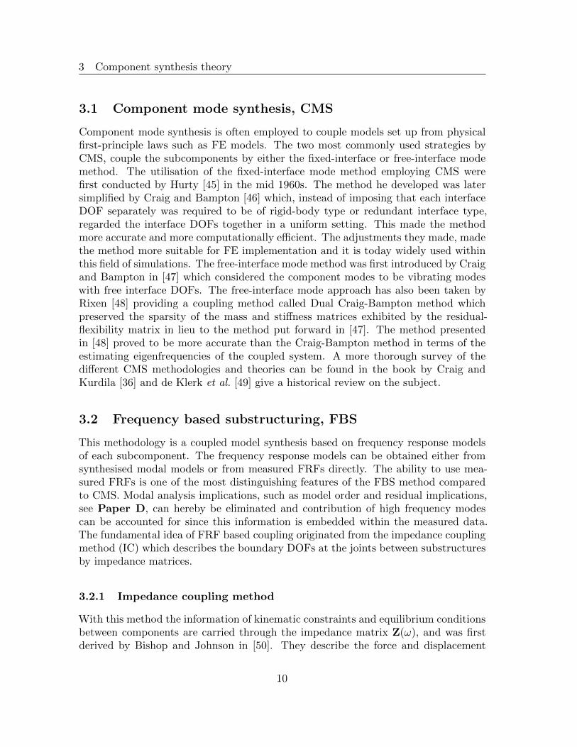
Component mode synthesis is often employed to couple models set up from physicalfirst-principle laws such as FE models. The two most commonly used strategies byCMS, couple the subcomponents by either the fixed-interface or free-interface modemethod. The utilisation of the fixed-interface mode method employing CMS werefirst conducted by Hurty [45] in the mid 1960s. The method he developed was latersimplified by Craig and Bampton [46] which, instead of imposing that each interfaceDOF separately was required to be of rigid-body type or redundant interface type,regarded the interface DOFs together in a uniform setting. This made the methodmore accurate and more computationally efficient. The adjustments they made, madethe method more suitable for FE implementation and it is today widely used withinthis field of simulations. The free-interface mode method was first introduced by Craigand Bampton in [47] which considered the component modes to be vibrating modeswith free interface DOFs. The free-interface mode approach has also been taken byRixen [48] providing a coupling method called Dual Craig-Bampton method whichpreserved the sparsity of the mass and stiffness matrices exhibited by the residual-flexibility matrix in lieu to the method put forward in [47]. The method presentedin [48] proved to be more accurate than the Craig-Bampton method in terms of theestimating eigenfrequencies of the coupled system. A more thorough survey of thedifferent CMS methodologies and theories can be found in the book by Craig andKurdila [36] and de Klerk et al. [49] give a historical review on the subject.

3.2 Frequency based substructuring, FBS

This methodology is a coupled model synthesis based on frequency response modelsof each subcomponent. The frequency response models can be obtained either fromsynthesised modal models or from measured FRFs directly. The ability to use mea-sured FRFs is one of the most distinguishing features of the FBS method comparedto CMS. Modal analysis implications, such as model order and residual implications,see Paper D, can hereby be eliminated and contribution of high frequency modescan be accounted for since this information is embedded within the measured data.The fundamental idea of FRF based coupling originated from the impedance couplingmethod (IC) which describes the boundary DOFs at the joints between substructuresby impedance matrices.

3.2.1 Impedance coupling method

With this method the information of kinematic constraints and equilibrium conditionsbetween components are carried through the impedance matrix Z(ω), and was firstderived by Bishop and Johnson in [50]. They describe the force and displacement

10

Summary of thesis

Figure 3: Illustration of coupling procedure. (a) Uncoupled subsystems I and II. (b)Kinematic and equilibrium constraints introduced. (c) Coupled system I+II

continuity through the coupling points between the assembled subsystems throughthe frequency dependant and complex-valued impedance matrix, Equation (10).

To utilise the impedance matrix in coupling of substructures it is needed to enforcecompatibility and equilibrium conditions, see Figure 3. The generalised responseco-ordinate of the assembled structure, qc, has to be coincident with the coupling

co-ordinates of the substructures to be assembled such that qcdef= qIc = qIIc and the

total external load applied to the interface DOFs of the assembly has to fulfil the

requirement that fcdef= f Ic + f IIc = f I,IIc + f Ic,e − f I,IIc + f IIc,e = f Ic,e + f IIc,e where f I,IIc

denotes the cross-sectional force between the two components and f Ic,e and f IIc,e arethe externally applied forces to the interface DOFs of components I and II.

These conditions can be written in matrix form with use of the transformation matrixT, for details see Ren and Beards [51], as

{qs} = T{qc} (16a)

{fc} = TT{fs} (16b)

11


where subscript s refers to the co-ordinates on the substructure. With Equation (10)rewritten as a matrix equation of subsystems

Zs(ω) {qs} = {fs} (17)

and with utilization of the compatibility and equilibrium conditions in Equation (16)a reformulation of Equation (17) can be established as

{qc} =(TTZs(ω)T

)−1

{fc} (18)

From Equation (18) it can see that the receptance matrix of the assembled systemH(ω) corresponds to

H(ω) =(TTZs(ω)T

)−1

(19)

This methodology fulfils all physical requirements needed through the compatibilityand equilibrium conditions but it is numerically inefficient as the method requires twomatrix inversions. First the subsystem receptance matrix Hs(ω) needs to be invertedto obtain the impedance matrix Zs(ω) and then a full size matrix inversion of Equation(19) is required. The inversion of the matrices makes this method especially sensitiveto measurement noise and matrix rank deficiencies which may cause significant errorsin the coupled model.

3.2.2 Generalised FRF impedance coupling technique

An alternative method to the IC-method were developed by Jetmundsen et al. in [27]where the number of required matrix inversions was reduced to one. This methodologyapplied to coupling of two subcomponents, I and II, provides the following matrixequation

H =

HIcc HI

co 0

HIoc HI

oc 0

0 0 HIIoo

−

HIcc

HIoc

-HIIoc

(HI

cc +HIIcc

)−1

HIcc

HIoc

-HIIoc

T

(20)

where H is the synthesised assembled receptance matrix and subscript (c) and (o)denotes interface and other DOFs respectively. It should be noted that the notationof H(ω) and Z(ω) have been changed to H and Z for brevity yet it is still implied thatH and Z are frequency dependent. A more general derivation of Equation (20) wasconducted by Ren and Beards in [51] to further utilise the concept of graph theory andmapping matrices, presented in [27] and [52] for the boolean operation of an arbitrary

12

Summary of thesis

number of substructures. The generalised FRF impedance coupling technique andthe coupling formulation in Equation (20) have been utilized in Papers B and E forevaluation purposes against the coupled results of state-space component synthesis.

3.3 State-space based coupling

The substructure synthesis method used to couple subcomponents in Papers A, Band E with improvements suggested in Papers C and D, has been the state-spacebased coupling technique proposed by Sjovall [53]. The state-space based couplingmethodology is closely related to FBS in that identical kinematic and equilibriumconstraints are enforced on the coupling. The state-space method approach to couplesubstructures was first taken by Su and Juang in [54] arguing several advantagescompared to FRF-based coupling methods. Some of the more prominent advantagesenlightened by [54] were the avoidance of ill-conditioned matrix inversions of the FRFmatrices and simplicity in identification on subsystem level with the estimation ofseveral lower order models. This is made rather than estimating a higher order modelthat is required for the coupled system level. The state-space based coupling methodproposed by [53] distinguishes itself from the method given by [54] in that it appliesproper similarity transformations of the subsystem state-space models in lieu to [54]that instead proposed an introduction of two additional auxiliary state variables toeach interface DOF. The method is described in fuller detail in Paper B.

13

4 Machining dynamics by component synthesis


Stability analysis for increased productivity and process reliability is used within themetal machining industry. However, the use is to some extent limited by a numberof factors. The methodology to employ stability lobe analysis requires experiencedusers to conduct the measurements of system transfer functions and to carry out thestability analysis. The use of the methodology is also affected by the requirements onthe measurement procedure. To obtain the correct dynamic flexibility at the tool tipfor a specific cutting tool it is required that the cutting tool is mounted in the machinetool of interest at test time. The use of a test rig or a FE representation of the machinetool have been proven insufficient in order to obtain the correct damping and stiffnessparameters of a machine tool. This is mainly due to the mechanical joint complexity ofthe machine tool structure. Furthermore the test procedure requires that the machinetool has to be taken out of operation during measurement. This results in loss ofvaluable production time. The productivity loss during measurements of a machinetool mounted cutting tools can be expensive for larger production plants. Largeproduction facilities can be equipped with more than 30 machine tools where eachmachine tool may carry a substantial amount of cutting tools due to the modularityof today’s tooling concepts, see Figure 4.

In an effort to reduce measurement time a number of researchers, see [18–26], haveutilised component synthesis to obtain the dynamic flexibility of a machine toolmounted cutting tool. The approach to the problem is to regard the cutting tooland the machine tool as two separate subsystems and then deploy component synthe-sis to construct the FRFs of transversal motion at the tool tip which are required forthe stability lobe prediction. Dividing the machine tool/cutting tool assembly intosubcomponents allows system identification to be conducted on subsystem level. Thismeans that the measurements of the machine tool dynamics only have to be conductedonce. The system description of the cutting tool, which is a less complex mechanicalcomponent, is normally made using analytical models of the tool in studies reported.

Figure 4: Machine tool modularity. This figure shows seven cutting tools but amagazine of a machine tool can hold up to over 100 cutting tools.

14

Summary of thesis

The substructuring approach to predict the tool tip dynamics was first taken bySchmitz and Donaldson [18]. The coupling was made on the measured machine toolsubcomponent FRFs to the analytically obtained FRFs of the free-free cylindricalcutting tool substructure directly utilizing the generalised FRF impedance couplingtechnique. In their work, the rotational degree of freedoms (RDOFs) were neglectedin the experimental characterisation of the coupling between the machine tool/toolholder subcomponents. An interface flexibility between the two subassemblies wereinstead introduced to compensate for the assumed joint flexibility between the toolholder and cutting tool. The introduction of the interface flexibility required an addi-tional measurement of a representative machine tool/tool holder mounted cutting toolto calibrate the interface flexibility properties. Their work was extended to include theRDOFs reported in Schmitz et al. [19]. However, these theoretical extensions werenot validated due to the absence of reliable measurement techniques of the RDOFFRFs.

The problem to obtain the RDOFs at the connection point on the machine toolsubstructure side was addressed in Park et al. [20]. Park made a different substructurepartition than made in [18, 19], by mounting a small part of the cutting tool insidethe tool holder. A measurement procedure was proposed that allowed the RDOFsto be obtained by measurements conducted on two blank calibration cylinders. Theproposed procedure was to conduct impact testing on one short blank cylinder and onelonger blank cylinder and then calculate the RDOFs at the free end of the short blankbased on these measurements using a decoupling procedure. The cutting tool FRFs atthe connection point were then constructed using an FE model of a cylindrical beamcoupled to connection point on the machine tool/tool holder/blank substructure. Thisapproach was later adopted by Namazi et al. [55] to retrieve the RDOFs closer to themachine tool spindle interface. This was achieved by partitioning the machine tooland a small part of the tool holder as one substructure and the tip of the tool holderand cutting tool as the other by applying the same experimental and decouplingmethods as proposed in [20]. The method proposed by Park has been benchmarkedin Paper E and the reader is referenced to that paper for further insight.

An alternative approach to retrieve the RDOFs at the connection point betweenmachine tool side of the substructures was taken by Schmitz and Duncan [22]. Themethodology they proposed included a triple-component coupling strategy where themachine tool and the base geometry of a tool holder were considered as one combinedsubstructure. The tip of the tool holder with the inserted part of the cutting toolconstituted another substructure and the part of the cutting tool outside of the toolholder was the third substructure. To obtain the RDOFs about the connection pointbetween the machine tool and tool holder base and the tip of the tool holder theyproposed a two step method. It consists of a first step in which measurements onthe translational DOFs at the free end of a machine tool mounted representative

15


tool holder were conducted. Then the RDOFs were calculated based on a receptancedecoupling method, from which the part of the general tool holder from the base tothe tip was subtracted. From these the machine tool/tool holder base receptancescould be obtained. In this work a synthesis of the RDOFs based on FRF data isalso proposed. This approach has also been subject of investigation in the benchmarkproblem presented in Paper E

A filtering method was applied in [22] to the measurements of the machine tool/toolholder with the aim to minimise the noise influence. The implication of noise contam-inated measurements on coupling of machine tool/cutting tools was further investi-gated by Schmitz and Duncan in [24]. They concluded that the noise contaminationmay strongly influence the results due to the matrix inversion made during the cou-pling of the FRFs. In Park and Chae [25] the approach on flexible joint descriptiontaken by Schmitz and Donaldson was combined with the method in [20] to accountfor the transfer function associated to the RDOFs of joints located adjacent to thetool tip. In [25] it was showed that this approach further could enhance the accuracyof the model of the coupled system.

4.1 Cutting tool model

In early substructuring attempts the cutting tool representations were made usingcylindrical beam models with a reduced diameter to compensate for the fluted geom-etry on solid carbide cutting tools. The influence of fluted geometry was addressedby Kivanc and Budak [56] where a derivation of moment of inertia considering 2, 3and 4 straight fluted solid carbide geometries was presented. The advantage of usingTimoshenko beam models rather than Euler-Bernoulli beam models to represent thecutting tool substructure was stressed in Erturk et. al. [23]. The advantage with theTimoshenko representation over the Euler-Bernoulli formulation is that the rotaryinertia and the shear deformation is considered. Especially the shear deformation isimportant to consider to increase accuracy in the calculated eigenvalues for cuttingtools with small length-to-diameter ratio, for details see Timoshenko et al. [33]. Theanalytical approach utilizing Timoshenko formulation of straight fluted cutting toolswas further developed by Mancisidor et al. [57], proposing a novel method utilizing acombination of clamped free and rigid body modes to establish a free-free represen-tation of the cutting tool. They showed that the number of modes required couldbe drastically reduced yet maintaining a high level of accuracy in the coupled results.Solid carbide cutting tool flutes are almost always helical to their design as the heli-cal shape facilitates ship evacuation and reduces sound levels in the cutting process.The helical shape was taken into consideration by Ozsahin and Altintas who utilizedthe moment of inertia description by Kivanc and Budak and divided the tool intodiscrete segments with fixed cross-section along the axial direction of the cutter. The

16

Summary of thesis

helical shape was approximated by sequential rotation of each segment and which alsopermitted for variations in flute cross section at different locations of the cutter.

The tool tip modelling approach taken in the appended Papers B through E dis-tinguishes itself from the approaches described which sits best for solid carbide tools.The solid carbide tool segment is indeed important but is small compared to sales ofindexable cutting tool. Indexable cutting tools often consists of a steel body on towhich small inserts are mounted. These inserts are active in the cutting process andcan consist of a variety of different materials such as coated solid carbide, ceramics,cubic boron nitride and in some cases even polycrystalline diamond. As the insert isworn down by machining, it is simply replaced by a new providing a more economicaltooling solution. An indexable cutting tool body differs, in some cases a lot, from therather continuous shape of a solid carbide cutter and to account for these variationsthe modelling approach has been based on appropriate FE models based on the CADmodels to represent its complex geometry. A CAD and FE model approach is slowerthan a strictly analytical approach with representative beam models but it enablesa more versatile analysis of tool geometric alterations in studies of the substructureresponse.

4.2 Substructure partition

Many of the articles cited within this application field have regarded flexible joints asa part of the modelling description. The necessity of such local flexibility is governedby the cutting tool design and the localisation of the interface between the cuttingtool and machine tool. A short example will be provided to illustrate the splittingaspect and how joint identification at the spindle and tool holder interfaces can becircumvented. Consider the defined system assembly in Figure 5.The presented structure is an extreme simplification of a machine tool, tool holderand cutting tool assembly, yet it is still valid to motivate the partitioning strategy

Figure 5: Assembly model

17


Table 1: Physical parameter values of damping and stiffness elements

i 1 2 3

mi [kg] 1 1 1

vi [Ns/m] 110 20 70

ki [kN/m] 3095 9870 9870

taken in this thesis. As seen, the simplified structure consists of three discrete inertiaelements, representing the machine tool, the tool holder and the cutting tool. Eachof them are sequentially connected with linear spring and damper elements and witha set of spring and damper element connected between the machine tool and ground.The intermediate stiffness and damper elements between the inertia represent flexiblejoints. The flexible joint between the machine tool spindle interface and tool holderhas been subject of investigation in Namazi et al. [55] and is represented by stiffnessand damping k2 and v2 and the joint flexibility between the tool holder and cuttingtool is represented by k3 and v3 in investigations presented in [18,19,21,22].

To enable a construction of the examples illustrating the different partitioning strate-gies a reference system (True) is established based on the assigned joint elementsvalues in Table 1 and the formation of the mass, stiffness and damping matrices as

MTrue =

m1 0 0

0 m2 0

0 0 m3

VTrue =

v1 + v2 −v2 0

−v2 v2 + v3 −v3

0 −v3 v3

, KTrue =

k1 + k2 −k2 0

−k2 k2 + k3 −k3

0 −k3 k3

(21)

18

Summary of thesis

Figure 6: Numerical substructure partition: Machine tool/tool holder as substructureI and cutting tool as substructure II

4.2.1 Machine tool/tool holder partition

A convenient substructure partition is to consider the machine tool and tool holderas one substructure and the cutting tool as a second substructure, see Figure 6. Apartitioning scheme such as this is attractive since it requires no splitting of exist-ing physical components. However, it has a downside in that the joint parametersbetween the tool holder and the cutting tools cannot be obtained in a single measure-ment session and need to be obtained through additional testing and joint parametercalibrations.

The necessity of additional testing will be illustrated in the following example. Thedynamic characteristics of the machine tool structure is, as previously argued, prefer-ably obtained by testing. In such testing, the machine tool mounted tool holder isnormally subjected to a short force impulse at DOF 2 (x2). In practice this is oftenmade by hammer excitation. For this example the impulse is constructed using anideal pulse filtered using a lowpass 2:nd order Butterworth filter with a cut-off fre-quency of 3000 Hz. The filtered impulse and the system response are sampled at arate of, fs = 1 MHz and the response is obtained using a digital filter representationof the system and ramp invariant transformation as proposed by Ahlin et al. [58], seeFigure 7.

19


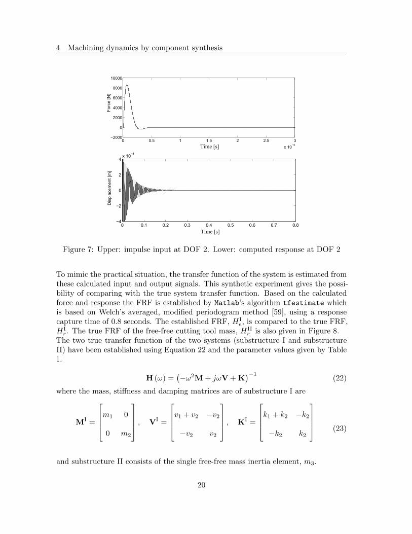
Figure 7: Upper: impulse input at DOF 2. Lower: computed response at DOF 2

To mimic the practical situation, the transfer function of the system is estimated fromthese calculated input and output signals. This synthetic experiment gives the possi-bility of comparing with the true system transfer function. Based on the calculatedforce and response the FRF is established by Matlab’s algorithm tfestimate whichis based on Welch’s averaged, modified periodogram method [59], using a responsecapture time of 0.8 seconds. The established FRF, HI

e, is compared to the true FRF,HI

r. The true FRF of the free-free cutting tool mass, HIIr is also given in Figure 8.

The two true transfer function of the two systems (substructure I and substructureII) have been established using Equation 22 and the parameter values given by Table1.

H (ω) =(−ω2M+ jωV+K

)−1(22)

where the mass, stiffness and damping matrices are of substructure I are

MI =

m1 0

0 m2

, VI =

v1 + v2 −v2

−v2 v2

, KI =

k1 + k2 −k2

−k2 k2

(23)

and substructure II consists of the single free-free mass inertia element, m3.

20

Summary of thesis

Figure 8: FRFs at coupling DOFs: Upper figure contains the true theoretical FRF,HI

r , and experimentally obtained FRF, HIe . Lower figure contains the theoretical

FRF of the free-free substructure II

As seen in Figure 8 in the comparison the correlation is good between the true andthe estimated FRFs of substructure I. The purpose of this comparison is to underlinethat the structural flexibility, including the structural flexible connection to groundand between spindle and tool holder, is embedded in the measured FRF.

As the joint information between the holder and cutting tool is missing the shortcom-ing of the experimental procedure becomes obvious by coupling of HI

e and HIIr using

Equation 20 and studding coupled results in comparison to the true assembled systemby applying MTrue, VTrue and KTrue to Equation 22, see Figure 9. Connecting thetwo substructures without considering the flexibility of the joint results in an assem-bled structure that is stiffer than the true systems. As such the system resonances arelocated at higher frequencies which in turn influences the accuracy of further cuttingprocess simulations and analysis.

An experimental set-up such as this hence requires that intermediate flexible jointelements are introduced between the tool holder and the cutting tool and that theseelements are calibrated using additional testing of a fully assembled structure, see[18, 19, 21, 22]. Once this is completed, substructuring of other cutting tools onto themachine tool/tool holder substructure can come in question.

21


Figure 9: Comparison of synthesis of, HIe and HII

r , and true assembled structureHTrue

r

Figure 10: Numerical substructure partition with integrated cutting tool partition

4.2.2 Integrated cutting tool partition

The problematic aspect regarding the missing joint description in the previous sectioncan be circumvented by adding a small portion of the cutting tool to the machinetool/tool holder substructure partition, see Figure 10. This approach was first takenin [20] and has been the substructure partition strategy taken in Papers A-E.

The benefit by this approach can be exemplified by adding a small part of the cuttingtool mass element, mI

3 = 0.1 [kg], (here named blank) to the machine tool/tool holderconfiguration. This corresponds to partitioning the cutting tool and mouthing theblank section in the tool holder. Next the example is continued by applying the sameinput force as presented in Figure 7, to DOF 3 of substructure I, calculate the responseand establish the FRFs in a similar fashion as presented in the previous section. Bythis partition the stiffness and damping matrices of substructure I are VI = VTrue

and KI = KTrue and the mass matrix MI, is

22

Summary of thesis

MI =

m1 0 0

0 m2 0

0 0 mI3

(24)

and substructure II consists of the single free-free mass inertia element, mII3 = 0.9

[kg], of the partitioned cutting tool mass.

The results of this procedure is provided in Figure 11. As seen, the experimentallyobtained FRF now consists of 3 modes as the joint flexibility between the tool holderand the cutting tool is considered in the experimental configuration (substructure I).By assembling substructure I and II it is now found that the match is good betweenthe synthesised FRF and the calculated true system, see Figure 12.

Figure 11: FRFs at coupling DOFs: Upper figure contains the true theoretical FRF,HI

r , and experimentally obtained FRF, HIe with integrated tool partition. Lower

figure contains the FRF of the free-free partition of the cutting tool (substructure II)

23


Figure 12: Comparison between substructured results of, HIe and HII

r , and true fullyassembled structure HTrue

r

As stated before the two examples presented here are extremely simplistic. In substruc-turing of a physical machine tool and cutting tool configuration both translational androtational DOFs need to be considered to appropriately capture the dynamic prop-erties at the coupling interface. The integrated cutting tool partition eliminates theneed for joint identification between the machine tool-tool holder-cutting tool but itdoes not eliminate the need for joint identification for all machine tool cutting toolcombinations. In configurations with joints near the tip of the tool, see Figure 13, atool tip adjacent joint identification still have have to be considered as suggested byPark and Chae [25]. No flexible joint descriptions has been considered in this thesisas no tooling solution of the sort where the joints of the substructures could not beintegrated in the experimental data have been considered. The focus has been onrobustness of the substructuring approach and on previously overlooked erroneousphenomenons and inconsistencies with physical principles.

Figure 13: Example of cutting tool solutions with joint adjacent to tool tip

24

Summary of thesis

5 Motivation to the state-space approach

Setting out from a numerical dynamic representation of sub-structures will result inthe same FRFs of the assembled structure using either one of the three approaches,CMS, FBS or state-space substructuring, see Papers B and D. The basic motivationto the used state-space approach is found in experimental obstacles that need to betackled and the ability to immediately utilize the coupled system model for analysis.This can be done in both time domain analysis of the cutting process and for analyticalstability lobe predictions. In experimental dynamic substructuring several obstaclesarise due to the inability to properly measure the dynamic characteristics of thesubsystems. Depending on which coupling method that is used these obstacles becomemore or less troublesome. Some of these obstacles have been mentioned above butwill be covered more in detail here.

5.1 Noise free data

As stated one of the most prominent features using FBS is that it can be applieddirectly onto measured data. This has been the most common approach in the field ofmachining dynamics by component synthesis. As much as this is a strength it is also aweakness in the sense it puts rather high demands on the quality of the measured data.To assure a robust and reliable coupled result the FRF data representations should befree from noise, [28,29]. As mentioned in section 4, Schmitz and Duncan [22], utilizeddata filtering to smooth the measured FRFs. Data smoothing is a well documentedtechnique to improve the accuracy and robustness of FBS. However, in the work byImregun et al. [60], it was shown that it is beneficial to have one consistent, reciprocalmodal model representation of the measured FRFs more so than fitting models tothe individual FRFs. A state-space formulation provides one such platform where aMIMO-FRF matrix could be identified and hereby also alleviating the noise effect.

5.2 Rotational degrees of freedom, RDOF

An appropriate description of the dynamic response of a structure requires both trans-lational and rotational DOF receptance formulation, Ewins and Gleeson [61]. How-ever, measurements of the RDOFs are rather cumbersome. Examples of cases whereRDOFs have been omitted can be found in literature, [20, 62]. These studies showedthat significant errors in amplitude and resonance frequency prediction of the cou-pled system may occur if the RDOFs were excluded. The problematic aspect liesin the practical problem to measure rotational response directly since there are norotational sensors on the market. A practical problem to obtain the full receptanceis also the problem of applying a torque excitation to the structure at a single pointof interest. An appropriate coupling point matrix contains FRFs of drive point andcross-coupling FRFs and can be subdivided in to four groups based on their input

25

5 Motivation to the state-space approach

and output characteristics. This is illustrated by the partition of the transfer functionmatrix H as

H =

HTF HTM

HRF HRM

(25)

Here subscripts T and F denotes response and excitation force respectively associatedto linear motion while R and M correspond to rotational response and moment exci-tation around a point. As seen in Equation (25), either a rotational excitation and/orresponse make up three quarters of the FRF matrix hence omitting the RDOFs resultsin significant information loss. Studies investigating the effect of excluding RDOFsin substructure coupling analysis have been reported in [62–64] and in experimentaldynamic substructuring of machine tool in particular in [20]. From these studies itcan be concluded that the RDOFs need to be included. This topic has been of interestto the experimental dynamic substructuring community for a long time and to somedegree still remains to be.

A number of different approaches could be found in the literature that aim to measurethe rotational responses as in the work by Bokelberg et al. [65,66]. A multi-directionaltransducer was developed, permitting response measurements in 6-DOFs by utiliza-tion of a laser vibrometer configuration with three laser beams. A similar strategyis the finite difference, (FD), approach which estimates the rotational response usingdifferentiation between closely spaced accelerometers, [28,63]. As these approach onlyserves to fill the first block column elements in Equation (25), complementary strate-gies need to be applied to synthesise the moment input elements. These right columnelements, HRM, can be synthesized by identification of a consistent model representa-tion and model expansion, Avitabile and O’Callahan [67]. As the state-space modelpermits for model expansion the FD approach in combination with model expansionhave been the most frequently used approach in Papers A-E. However, other meth-ods to synthesise the moment input elements using measured data directly can befound in the literature. Such approaches are often associated with a structural mod-ification, [20, 28, 68] where an additional component is attached to the experimentalsubstructure during testing. One of the more popular approaches is to attach a T-block to the experimental structure hereby allowing for both translational excitationand response to be measured at the ends of the T-block and the rotational responseand moment input can be synthesized by decoupling of the T-block. The structuralmodification method in [20] has been benchmarked in Paper E indicating high sensi-tivity to model properties of the decoupled modification structure and measurementaccuracy.

26

Summary of thesis

6 Experimental uncertainties

The substructuring approaches presented have different strengths and weaknesses andthey all share a common obstacle in measurement errors and uncertainties. The noiseissue have already been covered but errors such as sensor cross-axis sensitivity, cal-ibration errors and relocated sensor mass between measurements also need to beconsidered. In testing with shakers with stinger, stinger imperfections induce un-certain boundary conditions that contribute to uncertainties in the coupled results.Accelerometer mass and vibrating cables also participate to inaccuracies. These er-rors and inaccuracies are preferably addressed during the experimental work however,some of them may be hard to acknowledge and avoid in an industrial experimentalenvironment. One of the more important topics of this thesis is the establishment ofphysical consistent substructure models that partly adjust for experimental deficien-cies by avoiding model fitting to experimental data which are in conflict with physicalprinciples.

6.1 Test results inconsistent with principles of physics

Raw test data are usually processed by signal processing procedures. This may lead tofrequency response data estimates that are inconsistent with established fundamentalprinciples of physics. This subject, and its effects, have been sparsely covered in thefield of experimental substructuring. Among the first to acknowledge the phenomenonwere Carne and Dohrmann [69] who found that small measurement anomalies couldhave drastic effect, as spurious peaks frequently appeared in the frequency spectra ofthe coupled system. The artifacts in the estimated FRF are often hard/impossibleto find by simply studying the absolute value of the measured FRF but from closeexamination of the real and imaginary parts of driving point FRFs these anomaliescould often be located. In [69] comparisons are made between experimental andtheoretical accelerance MIMO FRF. Let the accelerance be represented by its realand imaginary parts as

Haij (ω) = ℜ

(Ha

ij (ω))+ jℑ

(Ha

ij (ω))

(26)

Based on real normal modes ϕ and natural frequencies ωn the real and imaginaryparts are (see [36])

27


ℜ(Ha

ij (ω))= −ω2

N∑

n=1

φinφjn

(1−

(ωωn

)2)

Kn

((1−

(ωωn

))2

+(2ζn

ωωn

)2) (27)

and

ℑ(Ha

ij (ω))= ω2

N∑

n=1

φinφjn

(2ζn

(ωωn

))

Kn

((1−

(ωωn

))2

+(2ζn

ωωn

)2) (28)

with Kn and ζn being the positive modal stiffness and damping respectively. By ex-amining the imaginary part it can be seen that the drive-point FRFs, i.e. when i = j,is positive if [ω,Kn, ζn] > 0. Further this implies that the phase of Ha

ij is boundedto stay between [0◦, 180◦]. As the frequency response can be represented in mobilityand receptance output as well the phase constraints for driving point FRF changesto [−90◦, 90◦] and [−180◦, 0◦] respectively and from being positive imaginary in theaccelerance case, to positive real in mobility and negative imaginary for receptanceoutput FRFs.

Figure 14 contains a receptance driving point measurement which exemplifies thesymptomatic errors found by Carne and Dohrmann, that have been an occurringphenomena in the experimental stages in the making of this thesis. Motivated bythe conclusions drawn from Equation (28) Carne and Dohrmann instead proposed atechnique named DeCompositon Data (DCD) filtering which eliminated most of thespurious peaks from the FBS prediction.The origin of the non-physical behaviour found in measurement data is of course ofhighest interest to the experimentalist. This behaviour is only attributed to eithernoise or subsequent mathematical prepossessing in [69]. The subject was furtherinvestigated in the context of state-space substructuring, by Sjovall and Abrahamssonin [70], and phase constrained state-space identification by McKelvey and Moheimaniin [31] where non-collocated and/or non-co-oriented sensors were acknowledged aspossible causes to the measurement phenomenon. A further plausible cause to thenon physical behaviour can also be found in data truncation of output signals. In thearticle by Trethewey and Cafeo, [32], the truncation effect is studied in FRFs obtainedfrom hammer tests.

28

Summary of thesis

Figure 14: Example of estimated phase, ∠, and imaginary, ℑ, part of drive pointaccelerance FRF from experimental test-rig examined in Papers A, C and D.

6.1.1 Truncation effects

A small example will be provided to illustrate the effects of output truncation thatwere enlightened by Trethewey and Cafeo. Considering one of the numerical struc-tures utilized in Paper D for residual compensation evaluation, Figure 15, where thephysical mass properties are mi = 1 [kg] and stiffness, ki, and damping, vi, are foundin Table 2.

Figure 15: Numerical/experimental structure

29


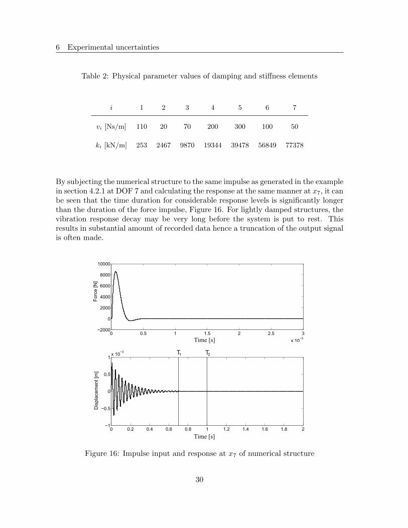
Table 2: Physical parameter values of damping and stiffness elements

i 1 2 3 4 5 6 7

vi [Ns/m] 110 20 70 200 300 100 50

ki [kN/m] 253 2467 9870 19344 39478 56849 77378

By subjecting the numerical structure to the same impulse as generated in the examplein section 4.2.1 at DOF 7 and calculating the response at the same manner at x7, it canbe seen that the time duration for considerable response levels is significantly longerthan the duration of the force impulse, Figure 16. For lightly damped structures, thevibration response decay may be very long before the system is put to rest. Thisresults in substantial amount of recorded data hence a truncation of the output signalis often made.

Figure 16: Impulse input and response at x7 of numerical structure

30

Summary of thesis

To study the point that Trethewey and Cafeo made, the FRFs are established us-ing Matlab’s tfestimate algorithm using two different capture times, T1 = 0.7s andT2 = 1s. These FRFs are compared to the theoretical FRF constructed, using Equa-tion (22) based on the values in Table 2 using M = I7×7 and were structure of thedamping, V and stiffens K matrices are

V =

v1 + v2 −v2 0 · · · 0

−v2. . .

. . .. . .

...

0. . .

. . . 0

.... . . v6 + v7 −v7

0 · · · 0 −v7 v7

K =

k1 + k2 −k2 0 · · · 0

−k2. . .

. . .. . .

...

0. . .

. . . 0

.... . . k6 + k7 −k7

0 · · · 0 −k7 k7

(29)

The results are found in Figure 17, from this it is evident that the FRF establishedusing the longer capture time is in good agreement to the true FRF. The FRF es-tablished using the shorter truncation time is however biased in both amplitude andphase. As seen the error is hard to detect in the amplitude plot without the assistanceof a reference yet the phase violation is more evident. The problem can indeed beminimized using an appropriate capture time, hitting the structure multiple times orapplying an exponential window on the response hereby artificially forcing a fasteramplitude decay yet is an important aspect to keep track of.

31


Figure 17: FRF magnitude and phase estimated with capture time T1 and T2 com-pared to theoretical reference, (Ref).

6.2 Physical model consistency

As measurement errors have been a documented problem in FBS, it may also havea devastating effect in state-space substructuring. If experimental errors occur it ishighly likely that these will be adopted by the state-space model. Noise contami-nation has been shown to be sufficient for causing non-physical state-space modelrepresentation in Sjovall and Abrahamsson, [70]. This leads to an unstable coupledmodel representations as a consequence. Continuing on the example from the previoussection it can be seen that the problem occurs when the FRF carries measurementanomalies that are other than noise. By subjecting the FRFs obtained using theT1 capture time to the unconstrained state-space subspace identification algorithmn4sid and the LSCP algorithm, an establishment of model representations on bothstate-space and residue and pole form is achieved. It can be seen in Figure 18 thatthe model captures the FRF data very well which means that it also captures thephase violating parts. It can also be seen that the two algorithms produces identicalFRFs which is not surprising since the state-space representation can be recast intoresidue and pole form, see Paper C.

32

Summary of thesis

Figure 18: FRF magnitude and phase estimated with capture time T1, identifiedstate space models (SYS) and residue-pole model (RP), compared to the theoreticalreference, (Ref).

The consequences of these measurement artifacts and the necessity to enforce pas-sivity constraints on subcomponent level, preventing the model from including thesemeasurement artifacts, are addressed in Papers C and D. By enforcing the proposedmethod in Paper C to the state-space model in the example it can be seen that thephase violation in the example is circumvented, see Figure 19.

6.3 Linear time-invariant systems

Passivity is one of the physical conditions enforced on the state-space subcompo-nent models in this thesis, yet others also follows based on the fundamental assump-tions that the structures studied are linear time-invariant (LTI), non-gyroscopic andnon-circulatory mechanical systems. Assumed as such, constraints can be placed onthe structure model representation such as causality, stability, reciprocity, passivity,displacement-velocity consistency and static mobility and accelerance response. Everysuch constraint is not a formidable obstacle to consider during the identification pro-

33


Figure 19: FRF magnitude and phase estimated with capture time T1 enforced pas-sivity, SYSp, compared to the theoretical reference, (Ref).

cess but to consider them all together has been shown cumbersome, Sjovall [53]. Ashort description of these rules will follow:

The first rule is causality which is fulfilled if the system’s output only depends onpresent and past inputs and not on future inputs. A state-space model representationas presented here, based on the real-valued quadruple, [A,B,C,D], is always causalhence this property is already defined by the model structure.

Stability is another expected property for the components treated here. A time-invariant system is said to be asymptotically stable if all poles of the system matrixA have negative real parts. This is a property that need to be imposed to the model.

Reciprocity, is fundamental in model expansion to synthesise unmeasured inputs andoutputs. Mechanical systems are expected to obey Maxwell-Betti’s reciprocity princi-ple, Meirovitch [71]. The reciprocity principle states that a system excited at locationi with measured response at location j is identical to the response at i if the same

34

Summary of thesis

excitation force is applied at j. Hence the following mathematical relation holds

Hij = Hji (30)

Passivity, much have been written within control theory about the mathematical con-ditions placed upon a transfer function such that it obeys the passivity criterion, seeBao and Lee [72]. In the context of an LTI, non-gyroscopic non-circulatory mechani-cal system, such as the ones studied in this thesis, the passivity criterion states thatthe system is passive if the total supplied power by any external loading to it, u,is positive. Further this implies that the real part of a mobility frequency transferfunction is positive real for all collocated and co-oriented inputs and outputs, i.e. alldriving point FRF elements, see [70] for proof. This is in line with the governingequations of real normal modes [36] and in analogy with this it also follows that theseFRF elements are bounded within the interval of [−90◦, 90◦]. As such the state-spacerepresentation of these elements are minimum phase, [72], hence all zeros and polesare located at the negative real plane. Note that system stability does not implypassivity.

Displacement-velocity consistency, regards Newton’s second law and places the re-striction upon the relation between input B and output C matrices of the state-spacemodel preventing a direct throughput term for velocity responses from applied forces.The subject is more thoroughly covered in Paper D but the consequence of the lawis that the input and output matrices for displacement response need to fulfil thefollowing condition CB=0.

The final condition regarding static mobility and accelerance response, is consideredfor mechanical structures that have no rigid body modes. The machine tool andexperimental test rig, which are fixed to ground, considered in this thesis are examplesof such. For these systems the velocity and accelerance response subjected to a staticload is zero and a condition on their related transfer function is that H (0) = 0. Theenforcement of this constraint is provided by the formulation of passivity enforcementin Paper C as this property can be satisfied for all modes of the system separatly.

35

7 Chatter vibrations in metal cutting


Chatter vibrations can occur in all metal cutting processes and is one of the mostcommon productivity limiting factors in metal machining. As such the ability toutilize the coupled results between the machine tool and cutting tool with respect topredictions of these vibrations is of highest priority. Comparisons between spindlespeed dependant stability limit, based on FRFs obtained from state-space componentsynthesis and reference measurements of the fully assembled structure have been done,Papers A, B and E, to evaluate the accuracy needed in the coupling prediction.Hence a more thorough coverage of this research field will follow.

Chatter occurs from dynamic force feed-back due to variation in chip thickness dur-ing cut. The variation in chip thickness originates from a phase shift in vibrationmarks left on the machined surface between two consecutive cuts. This phase shift isdependent on the dynamics of the machine tool/cutting tool assembly. The spindlespeed n and number of cutting teeth z govern the period time between cuts. Since thespindle speed is a process parameter to be selected by the operator, this parametercan be chosen so that the vibration marks from the previous cut is in phase with thecurrent cut. If the vibration marks between cuts is in phase then there will be no forcefeed-back and there will be no regenerative vibrations. A process optimisation withsupport in modelling and analysis is possible provided that the vibrational propertiesof the tool tip is known.

7.1 Chatter in turning of a disk

The simplest explanation model of chatter vibrations in the cutting process do regardorthogonal turning of a disk where the tool is fed in the radial direction of the disk.In case of a completely stable cutting process this example would provide that thefeed, fn, and the uncut chip thickness hD, would be the same. However, if the tool isto be considered to be flexible in the feed direction and a vibration is initiated fromthe entry of the cutting tool, the lamina formation of the chip or hardness variationsin the work piece material can cause forced oscillations. The vibration of the cuttingtool will then leave a wavy surface imprinted on the work piece. When the workpiece has turned one full revolution this waveform on the surface will result in avariation in chip thickness, hD(t), provided that there is a phase shift, ǫ, between theprevious and the currently cut surface. The time dependent chip thickness, hD(t), isin this case no longer constant with the feed per revolution fn, of the cutting tool.The chip thickness will instead be a function of the feed per revolution fn, the innermodulation, i.e current cut surface, y(t) and the outer modulation, i.e previously cutsurface, y(t− τ), see Figure 20.

The progression of the tool vibration under these conditions can take one of threeforms. The first case is a stable form where the vibration is damped out over time

36

Summary of thesis

Figure 20: Chip thickness variation in a turning process subjected to regenerativevibrations.

and the vibration amplitude diminishes. The second is when the vibration stayscritically stable and the vibration amplitude neither dampens out or grows and thethird is when the system becomes unstable and the vibrations grow to large levels.The last case is what is known in metal machining as chatter.

7.1.1 Stability lobe diagrams in turning

The most interesting case to predict, is the case when the process is critically stable.The first researchers to work actively to predict the stability limit for the turning casewere Tlustly [4] and Tobias [5]. They derived linear analytical expressions for predic-tion of chatter stability. They made a linearisation of the excitation force from thecutting process which permitted the stability equations to be derived in the Laplace

37


domain. From these an analytical expression for stability could be obtained. Bothresearchers stated that the cutting force acting in the feed direction, Ff(t), could beexpressed as a proportional relation between the edge length in cut, ap, the chip thick-ness, hD(t), and the work piece material dependent specific cutting force coefficient,kf, as

Ff(t) = kfaphD(t) (31)

From Figure 20 it can be concluded that the variation in chip thickness can be ex-pressed as hD(t) = fn + y(t − τ) − y(t), with τ being the time for one full turn ofthe work piece. Based on this conclusion the equation of motion of the system can beexpressed as

my(t) + cy(t) + ky(t) = kfap [fn + y(t− τ)− y(t)] (32)

The next step to derive an analytical expression for the critical stable system is totake the time invariant Delay Differential Equation (DDE) to Laplace domain. In theLaplace domain the current cut is expressed as, Y (s) = L(y(t)) and the previous cutis expressed as Y (s)esτ = L(y(t−τ)). The dynamic chip thickness in Laplace domainis therefore

hD(s) = fn + Y (s)esτ − Y (s) = fn + Y (s)(esτ − 1) (33)

and the dynamic cutting force in Laplace domain becomes

Ff(s) = kfaphD(s) (34)

The vibration excited by the dynamic cutting force can now be written as

Y (s) = Ff(s)H(s) = kfaphD(s)H(s) (35)

where H(s) = k + sc + s2m is the transfer function between the dynamic force andthe displacement. The relation between the dynamic chip thickness, hD(s) and thefeed per revolution fn can, by substituting the expression of Y (s) in Equation (35)into Equation (33), be expressed as

h(s)

fn=

1

1 + kfapH(s)(1− esτ )(36)

From Equation (36) the characteristic equation of the closed loop system is found tobe

1 + kfapH(s)(1− esτ ) = 0 (37)

38

Summary of thesis

The stability limit where the system is critically stable with respect to the edge lengthin cut, alimp , can after some manipulation of Equation (37), for details see [73], beshown to be

alimp =−1

2kfℜ(H(s))(38)

Here it can be seen that only negative values of the real part of the frequency responsefunction, ℜ(H(s)), produces valid results since alimp has to be positive. The spindlespeed and number of waves left on the work piece surface N , is related to frequencyω = −js, as

n =ω

60(2πN + ǫ)(39)

whereǫ = 3π + 2ψ

and for negative ℜ(H(s)),

ψ =

−π + tan−1

∣∣ℑHℜH

∣∣ if ℑH < 0

−π − tan−1∣∣ℑHℜH

∣∣ if ℑH > 0

Figure 21 shows how the solution of Equation (38) corresponds to the stability limitof the first stability lobe, i.e. N = 0.A stability lobe diagram for a specified spindle speed interval can now be created bysolving Equations (38)-(39) for a sufficient number of lobes N , see Figure 22.From Figure 22 it can be seen that some spindle speeds are better than others wherelarger edge lengths in cut, ap, can be machined without encountering chatter. It canalso be seen that for higher numbers of surface waves the closer the lobes get and thelesser the stability boundary for edge length in cut alimp varies with spindle speed.

7.2 Chatter in milling

Turning is usually a slow cutting process with a high tool tip resonance frequencywhich means that the number of vibration cycles during a full turn is large. This meansthat optimising a turning process with respect to chatter often given little room forimprovement. The milling process is more prone to improvements from spindle speedoptimisation and especially in the high speed machining segments. The main reasonthat the milling process can draw greater advantage from the stability optimisationis that the phase between the inner and outer surface modulations from one materialremoval cut is generated by two cutting teeth. Most of the commercial milling cuttershave more that one cutting tooth resulting in a tooth passing frequency which ishigher than the spindle revolution frequency. As a result of this, in combination

39


Figure 21: Relation between real part FRF ℜ(H(jω) and stability lobe for N = 0

Figure 22: Stability lobe diagram

with a more flexible cutting tool with lower resonance frequencies, a lower numberof vibration waves N needs to be considered for normal spindle speeds. This resultsin larger and wider stability lobes. The difference between ”good” and ”bad” spindlespeeds is therefore larger in terms of stable cutting edge length in cut ap, or axialdepth of cut which is the proper term in milling.

7.2.1 Stability lobe diagrams in milling

The chatter phenomenon in milling has many similarities to the related phenomenonin turning but there are some differences, both in terms of chatter mechanics andstability theory. The most significant difference between milling and turning is that

40

Summary of thesis

Figure 23: Illustration of a 2-DOF dynamic milling model considering transversalmotion in two directions. The figure defines the entering angle φst, and exiting angleφex in relation to the cutter and work piece. The dynamic chip thickness hD,m(t),is defined as the relation between the angle in cut φm, of tooth m and the dynamicdisplacement between the two consecutive teeth m− 1 and m.

in the milling process the cutting tool is rotating and not the work piece as it is inturning. This makes the theoretical assessment of stability lobe analysis somewhatmore cumbersome, since the cutting forces change both direction and amplitude dur-ing the cut. This is due to the change in orientation of the cutting tooth and variationin chip thickness, see Figure 23.

An analytical method to get the chatter stability diagram in milling was first derivedby Budak and Altintas [6, 7] who proposed a similar linearisation approach to thecutting force model as described in [4] and [5]. However, they included both thetangential and radial cutting forces, Ft,m and Fr,m, acting on the cutting tooth duringcut.

For the m:th tooth we have

41


Ft,m (t) = ktaphm (t) (40)

Fr,m (t) = kraphm (t) (41)

The angle dependent chip thickness hD,m (t), see Figure 23, can be approximated as

hD,m (t) =

{fz sinφm(t) + (υm-1 − υm) , φst < φm < φex

0, φex < φm < φst(42)

where fz sinφm(t) is the static chip thickness and υm and υm-1 is the dynamic dis-placements in radial direction of the m:th and (m− 1):th cutting teeth. Equation(42) can be expressed as a function of the tooth passing period τ , see Figure 24, as

hD,m (t) =

{fz sinφm(t) + (υ (t)− υ (t− τ)) , φst < φm < φex

0, φex < φm < φst(43)

With the assumption that there is no coupling between the radial and tangentialdegrees of freedom the total force contribution from all cutting edges z, can be written

Figure 24: Illustration of the dynamic chip thickness in milling as a function of thestatic feed dependent chip thickness fz sinφm(t). Here fz is the feed per tooth andφm is the angle in cut. It is also a function of the phase shift ǫ, which depend on thedynamic radial displacements υ (t) and υ (t− τ).

42

Summary of thesis

as

Fx (t) = −z−1∑

m=0

Ft,m (t) cosφm(t)−z−1∑

m=0

Fr,m (t) sinφm(t) (44)

Fy (t) =

z−1∑

m=0

Ft,m (t) sinφm(t)−z−1∑

m=0

Fr,m (t) cosφm(t) (45)

Here, the tangential and radial cutting forces have been projected to the table fixedcoordinate system xy, see Figure 23.

Equations (44) and (45) were used in [6] and [7] to derive equations (46) and (47) asthe foundation for the analytical stability lobe diagram of a milling process. Theseare for the axial depth of cut

alimp = −2πℜ(λ)zkt

(1− κ) (46)

where λ and κ can be found from

λ = − 1

2α0α1 ±

√α1 − 4α0

with

α0 = Hxx (jω)Hyy (jω) (αxxαyy − αxyαyx)

Hxx (jω) =1

−ω2M + jωcx + kx

Hyy (jω) =1

−ω2M + jωcy + ky

α1 = αxxHxx (jω) + αyyHyy (jω)

αxx =1

2

[cos 2φ− 2

krktφ+

krkt

sin 2φ

]φex

φst

αxy =1

2

[− sin 2φ− 2φ+

krkt

cos 2φ

]φex

φst

αyx =1

2

[− sin 2φ+ 2φ+

krkt

cos 2φ

]φex

φst

43


αyy =1

2

[− cos 2φ− 2

krktφ− kr

ktsin 2φ

]φex

φst

κ =ℑ(λ)ℜ(λ)

and the corresponding spindle speed is

n =60ω

z (ǫ+ 2πN)(47)

where the phase angle ǫ is

ǫ = π − 2ψ

and

ψ =

−tan−1∣∣∣ℑH(jω)ℜH(jω)

∣∣∣ if ℜH(jω) > 0, ℑH(jω) < 0

−π + tan−1∣∣∣ℑH(jω)ℜH(jω)

∣∣∣ if ℜH(jω) < 0, ℑH(jω) < 0

−π − tan−1∣∣∣ℑH(jω)ℜH(jω)

∣∣∣ if ℜH(jω) < 0, ℑH(jω) > 0

−2π + tan−1∣∣∣ℑH(jω)ℜH(jω)

∣∣∣ if ℜH(jω) > 0, ℑH(jω) > 0

Since the overall objective with the substructuring approach taken to the machinetool/cutting tool assembly is for process stability analysis the presented analyticalexpression for the stability lobes have been utilized for evaluation purposes in PapersA, B and E.

7.3 Time domain chatter stability boundary

The analytical chatter stability methods for obtaining stability lobe charts have bothadvantages and disadvantages. One great advantage is that the analytical methodsare fast. The two main phenomena the analytical methods does not consider are whenthe cutting tooth jumps out of the work piece due to excessive vibrations, and whenthe cutting force is strongly non-linearly related to feed or cutting speed. In thesecases time domain simulations produce better results. The time domain simulationapproach to predict chatter has been utilised by a number of researchers, see [8–17].The two most commonly used methods for time domain chatter stability predictionsare the Temporal Finite Element Analysis (TFEA) method, see [8, 9], and the Semi-Discretisation (SD) method, see [10–13].

44

Summary of thesis

The TFEA method compares the exact analytical solution for free tool vibration withan approximated solution of the tool vibrations during cut. The time-delay differentialequation has no closed form solution for the milling process so an approximatedsolution of the tool in cut is therefore established by dividing the time in cut into finitenumbers of time segments for the comparison. The two systems are then compared ina discrete linear map where the stability is determined by the characteristic multiplierof the map.

The SD method has been employed to approximate the delay differential equations(DDE) describing the stability of milling and turning operations by a series of ordinarydifferential equations (ODE). This is archived by approximating the time delay termsas piecewise constant functions.

The TFEA and SD methods have both been employed to predict stability lobe chartsfor a low radial immersion SDOF milling operation by Bayly et al. and Insperger et al.see [8] and [10]. Both methods were later extended to a more general 2 DOF millingoperation by Mann et al. [9] who used TFEA and Gradisek [14] who used the SDmethod. The various time domain methods, see [8–17], all differ from the analyticalmethods in that they have to be solved iteratively in order to find the stability bound-ary of the axial depth of cut alimp . Common to all investigations presented in [8–17], isalso that they all search for the bifurcation point, i.e. the limiting depth of cut werethe system becomes unstable. Different bifurcation types have been found to occurwith Hopf-bifurcation being the most common type. This usually manifests itself as achatter frequency close to a natural frequency of the system, see [11]. The second bi-furcation type observed using the TFEA method or the SD method is flip-bifurcationwhich is characterised by a chatter frequency at harmonics of odd multiples of half thetooth passing frequency, see [14]. The time-domain solutions of milling and turningprovides more information regarding the cutting process than the analytical methods.The time-domain simulation approach to the metal cutting process can be extendednot only to determine chatter but also to quantify the severity of the vibrations andbe used to predict surface texture during stable and unstable conditions, see [74].

45

8 Summary of appended papers

8 Summary of appended papers

Paper A: Dynamic substructuring in metal cutting machine chatter

The RDOF using a single experimental set-up is addressed using system identificationand model expansion taking the conceptual approach of experimental dynamic testingand system identification on state space form. The experimental set-up was appliedto a physical test rig. The state-space coupling algorithms were employed to couplethe identified test rig structure to a synthesised subsystem representing the cuttingtool. The model of the cutting tool was based on the mass and inertia propertiesretrieved from a CAD model tool. The experimental set-up combined with systemidentification and model expansion allowed for the experimentally obtained systemmodel and the assembled structure model to contain a five degree of freedom modelrepresentation. This was an expansion of the frequency response function matrix de-scribing the coupled system to include also cross FRF relations between the five DOFswhich was novel at the time. The synthesised FRFs of the assembled substructureswere compared and evaluated against measurements of the fully assembled test rigwith encouraging yet not fully satisfactory results.

Paper B: Experimental-analytical substructure model sensitivity analysis for cuttingmachine chatter prediction

A sensitivity analysis of parameter influence on the coupled system was conducted.A number of parameters related to the identification process were perturbed in orderto see the magnitude of influence each parameter had on the coupled system. Theeffect of perturbation of parameters such as state-order, FRF response magnitude,damping estimation and frequency cut-off were investigated. A reference system wasconstructed based on an FE model of the test rig used in Paper A and the parameterinfluence investigation was conduced based on perturbations of the reference system.Concluded from the output of the study is that an appropriate state order is of theessence in model based substructuring. A more general conclusion applied to allcoupling methods is that the amplitude of the frequency response functions stronglyinfluences the coupled results hence puts high demands on the experimental accuracyand sensor calibration.

46

Summary of thesis

Paper C: Dynamic sub-structuring with passive state-space components

Unstable poles found in the coupled system models are addressed. The problem isfound in coupled system model presented in Paper A in which one of the systemmodels is obtained based on experimental dynamic testing and system identification.The problem could not be observed in Paper B where both subcomponents originatesfrom physically consistent FE data. The problem hinders time domain simulations ofthe coupled results and the problem was found to originate from passivity violationsof the experimentally obtained state-space models. The paper addresses this issue andpresents a novel method to enforce passivity and static mobility response stationarityfor constrained MIMO mobility FRFs resulting in state space subsystem models takento a driving point minimum phase state, hereby assuring model stability leading tonumerical stability.

Paper D: Residual compensation in experimental state space model synthesis

The modal incompleteness aspect of identified state-space models is taken into con-sideration. The modal contribution of modes outside the measured frequency intervalinfluences the coupled results and compensation strategies can be found on other sys-tem model descriptions but not for a state-space formulation. A developed method toaccount for both high and low frequency residuals of state space models is presentedand integrated in the overall coupling strategy that assures physical consistency ofthe coupled state-space models. The results are evaluated on both numerical andexperimental data showing improvements on coupled results against reference modelsand measurements. An interesting finding presented is that modal incompletenessmay lead to passivity violation.

Paper E: On rotational degrees of freedom for substructure synthesis of machine tooland cutting tools

The developed experimental test and coupling strategy as presented in, Papers A-D,is finally evaluated on a physical machine tool. The paper emphasis is on the evalua-tion of the most suitable experimental and theoretical method to synthesize rotationaldegrees of freedom. The methods proposed by [20] and [22] are compared to the de-veloped coupling method. It lifts overlooked erroneous phenomenons, symptomaticto each investigated strategy, occurring in the synthesised RDOF FRFs and presentsprobable causes and the effect these have on the coupled system. The evaluation isperformed on both analytical and experimental structures.

47

9 Conclusions and future work

9 Conclusions and future work

A method for component synthesis of machine tool and cutting tool assemblies basedon experimentally and numerically obtained state-space subcomponents has been pre-sented. The emphasis has been on robustness and generality of the coupling procedureand lifts and addresses challenging aspects originating from both the experimental andmodelling sides. The robustness aspects lies in the ability to assure a model descrip-tion on coupled form that is fit for further analysis and holds the properties expectedfrom a general LTI, non-gyroscopic, non-circulatory stable system. The developedmethodology is hereby not solely devoted to machine tool structures.

It has been experienced that the truly challenging aspect of experimental dynamicsubstructuring that effects the accuracy the most is in the experimental part. Theproposed method has been shown to sufficiently assist in metal cutting stability pre-dictions, however, the inability to properly measure the rotational degrees of freedom,response errors inherited by signal processing, placement and calibration errors ofsensors and so on, all contribute to uncertainties of the magnitude that may easilyovershadow the predicted results. The proposed method constrains the substructuremodel description from violation of well defined physical principles, and was foundto fundamentally influence the state-space coupling results. This makes the coupledresults more robust, yet it will never fully compensate for poor measurement results.

A compensation method for mode contributions outside the measured frequency rangehave been addressed. The methodology has further been successfully implemented inthe overall methodology to assure a physically consistent state-space coupled result.The taken approach has been shown to improve the prediction of eigenvalue and an-tiresonance locations still maintaining a stable and passive coupled state-space model.

Expansion strategies to establish unmeasured FRF elements in both frequency domainand on state-space model form have been a subject of investigation. The differencesthese strategies impose have been evaluated on both subcomponent level and on cou-pled form. From this evaluation it can be concluded that the generation of RDOFsin the frequency domain by decoupling is extraordinary sensitive to model and exper-imental errors.

The overall objective to, develop a robust experimentally based coupling approach tosynthesise machine tool and cutting tool structures has been met. However, improve-ment potential can be identified on a number of accounts. From the experimentalevaluation regarding the residual compensation strategy, presented in Paper D, abetter strategy to find the optimal number and location of the compensational polesshould be made instead of the ad hoc method used in the paper. Such approach wouldfurther be of interest for the identified shortcoming in Paper E where it was foundthat the placement of moment to rotational response antiresonances are governed bythe location of the compensational modes.

48

Summary of thesis

References

[1] T. Surmann and D. Enk. Simulation of milling tool vibration trajectories alongchanging engagement conditions. International Journal of Machine Tools andManufacture, 47(9):1442–1448, 2007.

[2] T. Surmann and D. Biermann. The effect of tool vibrations on the flank sur-face created by peripheral milling. CIRP Annals - Manufacturing Technology,57(1):375–378, 2008.

[3] C. Eksioglu, Z.M. Kilic, and Y. Altintas. Discrete-time prediction of chatterstability, cutting forces, and surface location errors in flexible milling systems.Journal of Manufacturing Science and Engineering, 134(6), 2012.

[4] J. Tlustly and M. Polacek. The stability of machine tools against self ex-cided vibrations in machining. International Research in Production Engineering,ASME:465–474, 1963.

[5] S.A. Tobias. Machine Tool Vibrations. Blackie and Sons Ltd., 1965.

[6] E. Budak and Y. Altintas. Analytical prediction of chatter stability in milling—part i: General formulation. Journal of Dynamic Systems, Measurement, andControl, 120(1):22–30, 1998.

[7] E. Budak and Y. Altintas. Analytical prediction of chatter stability in milling—part ii: Application of the general formulation to common milling systems. Jour-nal of Dynamic Systems, Measurement, and Control, 120(1):31–36, 1998.

[8] P.V. Bayly, B.P. Mann, T.L. Schmitz, D.A. Peters, S. Gabor and T. Insperger.Effects of radial immersion and cutting direction on chatter instability in end-milling. In Proceedings of IMECE 2002, ASME International Mechanical Engi-neering Congress and Exposition, New Orleans, Louisiana, 2002.

[9] B.P. Mann, P.V. Bayly, M.A. Davies, and J.E. Halley. Limit cycles, bifurcations,and accuracy of the milling process. Journal of Sound and Vibration, 277(1-2):31– 48, 2004.

[10] T. Insperger, B.P. Mann, G. Stepan, and P.V. Bayly. Stability of up-milling anddown-milling, part 1: alternative analytical methods. International Journal ofMachine Tools and Manufacture, 43(1):25 – 34, 2003.

[11] T. Kalmar-Nagy, S. Gabor, and F. Moon. Subcritical hopf bifurcation in thedelay equation model for machine tool vibrations. Nonlinear Dynamics, 26:121–142, 2001.

49

References

[12] T. Insperger, D.A.W. Barton, and G. Stepan. Criticality of hopf bifurcationin state-dependent delay model of turning processes. International Journal ofNon-Linear Mechanics, 43(2):140 – 149, 2008.

[13] T. Insperger and G. Stepan. Chatter suppression of turning process via periodicmodulation of the spindle speed - a 1 dof analysis. In Proceedings of the ThirdConference on Mechanical Engineering, Budapest, Hungary, 2002.

[14] J. Gradisek, M. Kalveram, T. Insperger, K. Weinert, G. Stepan, E. Govekar, andI. Grabec. On stability prediction for milling. International Journal of MachineTools and Manufacture, 45(7–8):769 – 781, 2005.

[15] M.X. Zhao and B. Balachandran. Dynamics and stability of milling process.International Journal of Solids and Structures, 38(10-13):2233 – 2248, 2001.

[16] J. Gradisek, E. Govkar, and I. Grabec. Chatter onset in non-regenerative cutting:A numerical study. Journal of Sound and Vibration, 242(5):829 – 838, 2001.

[17] A. Ganguli. Chatter reduction through active vibration damping. PhD thesis,Universite Libre De Bruxelles, Bruxelles, Belgium, 2005.

[18] T.L. Schmitz and R.R. Donalson. Predicting high-speed machining dynamicsby substructure analysis. CIRP Annals - Manufacturing Technology, 49(1):303 –308, 2000.

[19] T.L. Schmitz, Matthew A.D., and Michael D.K. Tool point frequency responseprediction for high-speed machining by RCSA. Journal of Manufacturing Scienceand Engineering, 123(4):700–707, 2001.

[20] S.S. Park, Y. Altintas, and M. Movahhedy. Receptance coupling for end mills.International Journal of Machine Tools and Manufacture, 43(9):889 – 896, 2003.

[21] T. Schmitz. Receptance coupling for high-speed machining dynamics prediction.Proceedings of the 21st International Modal Analysis Conference, pages 1–12,2003.

[22] T.L. Schmitz and G.S. Duncan. Three-Component Receptance Coupling Sub-structure Analysis for Tool Point Dynamics Prediction. Journal of ManufacturingScience and Engineering, 127(4):781, 2005.

[23] A. Erturk, H. Ozguven, and E. Budak. Analytical modeling of spindle – tool dy-namics on machine tools using Timoshenko beam model and receptance couplingfor the prediction of tool point FRF. International Journal of Machine Tools andManufacture, 46(15):1901–1912, 2006.

50

Summary of thesis

[24] T. Schmitz and G. Duncan. Receptance coupling for dynamics prediction ofassemblies with coincident neutral axes. Journal of Sound and Vibration, 289(4-5):1045–1065, 2006.

[25] S.S. Park and J. Chae. Joint identification of modular tools using a novel recep-tance coupling method. The International Journal of Advanced ManufacturingTechnology, 35(11-12):1251–1262, 2008.

[26] I. Mancisidor, M. Zatarain, J. Munoa, and Z. Dombovari. Fixed BoundariesReceptance Coupling Substructure Analysis for Tool Point Dynamics Prediction.Advanced Materials Research, 223:622–631, 2011.

[27] B. Jetmundsen, R. L. Bielawa andW.G. Flannelly. Generalized frequency domainsubstructure synthesis. Journal of the American Helicopter Society, 33(1):55–64,1988.

[28] D.J. Ewins. Modal Testing: Theory, Practice and Application. Research studiespress LDT., 2001.

[29] M.L.M Duarte. Experimentally-derived structural models for use in further dy-namic analysis. PhD thesis, University of London London, 1996.

[30] T. Lim. A Theoretical and Computational Study of the FRF-Based Substructur-ing Technique Applying Enhanced Least Square and TsvdApproaches. Journal of Sound and Vibration, 231(4):1135–1157, 2000.

[31] T. McKelvey and S.O.R. Moheimani. Estimation of phase constrained MIMOtransfer functions with application to flexible structures with mixed collocatedand non-collocated actuators and sensors. In World Congress, volume 16, pages36–36, 2005.

[32] M.W. Trethewey and J.A. Cafeo. Tutorial: signal processing aspects of structuralimpact testing. The International Journal of Analytical and Experimental ModalAnalysis, 7(2):129–149, 1992.

[33] S. Timoshenko, D.H. Young, and W. Weaver. Vibration Problems in Engineering,volume 208. John Wiley and Sons, Inc., 1990.

[34] V. Kolousek, R.F. McLean, and J.S. Fleming. Dynamics in engineering structures.Butterworths, London, 1973.

[35] N. Saabye and H. Petersson. Introduction to the Finite Element Method. PrenticeHall Internationa, 1992.

[36] R.R. Craig and A.J. Kurdila. Fundamentals of Structural Dynamics. Wiley, 2006.

51

References

[37] W.K. Gawronski. Dynamics and control of structures: a modal approach.Springer, New York, 1998.

[38] M.I. Friswell, J.E. Mottershead, SpringerLink (Online service), and Springer-Link Archive (e-book collection). Finite Element Model Updating in StructuralDynamics, volume 38. Springer Netherlands, Dordrecht, 1995.

[39] L. Ljung. System Identification: Theory for the User (2nd Edition). PrenticeHall PTR, 1998.

[40] P. Overschee, B. Moor, SpringerLink (Online service), and SpringerLink Archive(e-book collection). Subspace Identification for Linear Systems: Theory - Imple-mentation - Applications. Springer US, Boston, MA, 1996.

[41] A. Brandt. Noise and vibration analysis: signal analysis and experimental proce-dures. Wiley, Chichester; Hoboken, N.J, 2011.

[42] N.M.M. Maia. Extraction of Valid Modal Properties from Measured Data inStructural Vibrations. University of London, 1988.

[43] T. McKelvey, H. Akcay, and L. Ljung. Subspace-based multivariable systemidentification from frequency response data. IEEE Transactions on AutomaticControl, 41(7):960–979, 1996.

[44] V. Yaghoubi and T. Abrahamsson. Automated modal analysis based on frequencyresponse function estimates. In R. Allemang, J. De Clerck, C. Niezrecki, and J.R.Blough, editors, Topics in Modal Analysis I, Volume 5, Conference Proceedingsof the Society for Experimental Mechanics Series, pages 9–18. Springer New York,2012.

[45] W.C. Hurty. Dynamic analysis of structural systems using component modes.AIAA Journal, 3(4):678–685, 1965.

[46] R.R. Craig, Jr. and M.C.C. Bampton. Coupling of substructures for dynamicanalysis. AIAA Journal, 6(7):1313–1319, 1968.

[47] R.R. Craig, Jr. and M.C.C. Bampton. On the use of attachment modes in sub-structure coupling for dynamic analysis. In AIAA/ASME 18th Structures, Struc-tural Dynamics and Materials Conference, San Diego, CA, 1977.

[48] D.J. Rixen. A dual Craig-Bampton method for dynamic substructuring. Journalof Computational and Applied Mathematics, 168(1-2):383–391, 2004.

[49] D.D. Klerk, D.J. Rixen, and S.N. Voormeeren. General framework for dynamicsubstructuring: History, review and classification of techniques. AIAA Journal,46(5):1169–1181, 2008.

52

Summary of thesis

[50] R.E.D. Bishop and D.C. Johnson. The mechanics of vibration. Cambridge Uni-versity Press, Cambridge, 1960.

[51] Y. Ren and C.F. Beards. On substructure synthesis with frf data. Journal ofSound and Vibration, 185(5):845–866, 1995.

[52] B. Jetmundsen. On frequency domain methodologies for prescribed structuralmodification and subsustem sysnthesis. PhD thesis, Rensselaer Polytechnic Insti-tute, Troy, New York, 1986.

[53] P. Sjovall. Identification and Synthesis of Components for Vibration TransferPath Analysis. PhD thesis, Chalmers University of Technology, Gothenburg,Sweden, 2007.

[54] T.J. Su and J.N. Juang. Substructure system identification and synthesis. Jour-nal of Guidance, Control and Dynamics, 17(5):1087–1095, 1994.

[55] M. Namazi, Y. Altintas, T. Abe, and N. Rajapakse. Modeling and identificationof tool holder—spindle interface dynamics. International Journal of MachineTools and Manufacture, 47(9):1333 – 1341, 2007.

[56] E.B. Kivanc and E. Budak. Structural modeling of end mills for form errorand stability analysis. International Journal of Machine Tools and Manufacture,44(11):1151 – 1161, 2004.

[57] I. Mancisidor, A. Urkiola, R. Barcena, J. Munoa, Z. Dombovari, and MikelZatarain. Receptance coupling for tool point dynamic prediction by fixed bound-aries approach. International Journal of Machine Tools and Manufacture, 78:18– 29, 2014.

[58] K. Ahlin, M. Magnevall, and A. Josefsson. Simulation of forced response inlinear and nonlinear mechanical systems using digital filters. In InternationalConference on Noise and Vibration Engineering (ISMA2006). Katholieke univ.Leuven, Dept. Werktuigkunde, 2006.

[59] P. Welch. The use of fast fourier transform for the estimation of power spectra:A method based on time averaging over short, modified periodograms. IEEETransactions on Audio and Electroacoustics, 15(2):70–73, 1967.

[60] M. Imregun, D.A. Robb, and D.J. Ewins. Structural Modification and CouplingDynamic Analysis Using Measured FRF Data, In 5th International Modal Anal-ysis Conference IMAC V, London, 1987.

[61] D.J. Ewins and P.T. Gleeson. Experimental determination of multidirectionalmobility data for beams. Shock and Vibration Bulletin, 5:153–173, 1975.

53

References

[62] W. Liu and D. Ewins. The importance assessment of rdof in frf coupling analysis.In Proceedings of the Seventeenth International Modal Analysis Conference, pages1481–1487. Citeseer, 1999.

[63] M.L.M Duarte and D.J. Ewins. Some insights into the importance of rota-tional degrees-of-freedom and residual terms in coupled structure analysis. InProceedings-Spite The International Society for Optical Engineering, pages 164–170. Leuven (Belgium), 1995.

[64] T. Gialamas, D. Tsahalis, L. Bregant, D. Otte, and H. Van der Auweraer. Sub-structuring by means of frfs: some investigations on the significance of rotationaldofs. In Proceedings-Spite the international society for optical engineering, 619–625,1996.

[65] E.H. Bokelberg, H.J. Sommer III, and M.W. Trethewey. A six-degree-of-freedomlaser vibrometer, part i: theoretical development. Journal of sound and vibration,178(5):643–654, 1994.

[66] E.H. Bokelberg, H.J. Sommer III, and M.W. Trethewey. A six-degree-of-freedomlaser vibrometer, part ii: Experimental validation. Journal of Sound and Vibra-tion, 178(5):655 – 667, 1994.

[67] P. Avitabile and J. O’Callahan. Frequency response function expansion for un-measured translation and rotation dofs for impedance modelling applications.Mechanical Systems and Signal Processing, 17(4):723 – 745, 2003.

[68] D. Montalvao, A.M.R. Ribeiro, N.M.M. Maia, and J.M.M. Silva. Estimationof the rotational terms of the dynamic response matrix. Shock and Vibration,11(3-4):333–350, 2004.

[69] T.G. Carne and C.R. Dohrmann. Improving experimental frequency responsefunction matrices for admittance modeling. In Proceedings of the NineteenthInternational Modal Analysis Conference, 2006.

[70] P. Sjovall and T. Abrahamsson. Component system identification and state-spacemodel synthesis. Mechanical Systems and Signal Processing, 21(7):2697–2714,2007.

[71] L. Meirovitch. Principles and techniques of vibrations. Prentice Hall, UpperSaddle River, N.J, 1997.

[72] J. Bao and P.L. Lee. Process Control: The Passive Systems Approach (Advancesin Industrial Control). Springer Verlag London Limited, 1. aufl. edition, 2007.

[73] Y. Altintas. Manufacturing Automation: Metal Cutting Mechanics, MachineTool Vibrations and CNC Design. Cambridge University Press, 2000.

54

Summary of thesis

[74] K. Weinert, T. Surmann, D. Enk, and O. Webber. The effect of runout on themilling tool vibration and surface quality. Production Engineering, 1:265–270,2007.

55

J +?BM2 hQQH .vM KB+b - CORE

Documents

Transcript of J +?BM2 hQQH .vM KB+b - CORE