IWRAP MK II WORKING DOCUMENT BASIC MODELLING … · predicted too many events and a correction...
59
IWRAP MK II WORKING DOCUMENT BASIC MODELLING PRINCIPLES FOR PREDICTION OF COLLISION AND GROUNDING FREQUENCIES: Date: 2007.08.01 Rev. 4: 2008.03.09 Peter Friis-Hansen Technical University of Denmark
Transcript of IWRAP MK II WORKING DOCUMENT BASIC MODELLING … · predicted too many events and a correction...

IWRAP MK II
WORKING DOCUMENT
BASIC MODELLING PRINCIPLES FOR PREDICTION OF COLLISION AND
GROUNDING FREQUENCIES:
Date: 2007.08.01 Rev. 4: 2008.03.09
Peter Friis-Hansen
Technical University of Denmark

Collision and Grounding frequency Page 2 of 59
Date: 03/09/2008
TABLE OF CONTENTS
1. BACKGROUND .......................................................................................................................... 3 2. INTRODUCTION.......................................................................................................................... 3 3. PROBABILISTIC COLLISION AND GROUNDING ANALYSIS............................................................... 5 3.1 Risk models ............................................................................................................................ 5 4. PREDICTING COLLISION AND GROUNDING FREQUENCIES............................................................. 7 4.1 Frequency of collision............................................................................................................. 7 4.1.1 Head-on and overtaking collisions......................................................................................... 8 4.1.2 Crossing collisions................................................................................................................10 4.1.3 Collision test cases...............................................................................................................15 4.2 Probability of grounding........................................................................................................22 4.2.1 Powered grounding ..............................................................................................................24 4.2.2 Drifting grounding .................................................................................................................26 4.3 Assessing the traffic spread across the route......................................................................28 4.4 Calculation procedure for estimating the collision frequency..............................................28 4.5 Combined causation factor jiCP , ........................................................................................29 5. CAUSATION PROBABILITY........................................................................................................29 5.1 Causation probabilities from literature .................................................................................30 5.2 Risk model for obtaining the causation probability ..............................................................32 5.2.1 Traditional approach.............................................................................................................33 5.2.2 Using Bayesian Networks ....................................................................................................33 5.2.3 Bayesian Network for ship-ship collisions............................................................................36 5.3 Default values used in GRISK..............................................................................................39 6. FACTORS THAT INFLUENCE THE CAUSATION PROBABILITY ........................................................39 6.1 Reported causes for grounding and collision ......................................................................39 6.1.1 Human and Organisational Errors .......................................................................................40 6.1.2 Human error evaluation........................................................................................................41 6.2 Aspects that the risk analysis should include ......................................................................42 6.2.1 Configuration of navigational area .......................................................................................43 6.2.2 Composition of ship traffic ....................................................................................................45 6.2.3 Environmental conditions .....................................................................................................46 6.2.4 Configuration of considered vessel......................................................................................46 7. SHIP TYPES USED IN THE GRISK PROGRAM ............................................................................48 8. CONCLUSION ..........................................................................................................................48 9. REFERENCES..........................................................................................................................49
Collision and Grounding frequency Page 3 of 59
Date: 03/09/2008
1. BACKGROUND The objective of the present report is to describe the theoretical background for the collision and grounding frequency analysis that forms the basis of the IWRAP MK II program. The IWRAP MK II constitutes a reduced version of the collision and grounding analysis program, The BaSSy ToolBox (GRISK) that is being developed under the BaSSy-project. The BaSSy project is a joint research project between Technical University of Denmark, GateHouse (Denmark), SSPA (Sweden), and VTT (Finland), which is funded in part by The Danish Maritime Foundation and Det Nordiske Ministerråd. The objective of the present report is to describe the theoretical foundation for the collision and grounding frequency analysis so that the interested user of IWRAP MK II may understand the fundament behind the program. It is assumed that the reader assumes a level of mathematical and probabilistic skills to gain full benefit of the report.
2. INTRODUCTION To quantify the risks involved with vessel traffic in specified geographical areas, rational criteria for prediction and evaluation of grounding and collision accidents have to be developed. This implies that probabilities as well as the inherent consequences have to be analysed and assessed. During the period from 1998 to 2001 state-of-the-art software for grounding and collision analysis that was developed within the ISESO project at the Technical University of Denmark. The ISESO project was conceived by the Danish Maritime Authority (Søfartsstyrelsen) in co-operation with Danish maritime industries and trades. The purpose of ISESO was to develop front-end technological maritime simulation tools for the benefit of Danish shipping, and the aim has been to contribute to maintaining and extending the Danish position within this area of commercial activity. The acronym ISESO stands for Information Technology for Increased Safety and Efficiency in Ship Design and Operation (in Danish: “Informationsteknologi i forøget Sikkerhed og Effektivitet i Skibsdesign og –Operation”), see www.iseso.org for more information. One of the objectives of the ISESO project was to develop a software package of rational tools for streamlining and assisting in applying FSA methods. The developed computer program, GRACAT (Grounding and Collision Analysis Toolbox) facilitates these types of analyses and further provides rational tools for evaluating and comparing the grounding and collision risk for the analysed alternatives. The software calculates the probability of collision or grounding for a vessel operating on a specified route. Given that a collision or grounding event has taken place the spatial distribution of the damages to the hull may further be calculated. Results are presented in terms of probability distributions for indentation depth, length and height of the damage and for their location. A special case of a probabilistic analysis is a purely deterministic analysis, which also may be performed within GRACAT. Results for accident frequency and damage have been compared to registered data and good agreement was found in all cases. The procedures developed during the development of GRACAT constitutes an essential part of the BaSSy project and thus also of the program with the working title “IWRAP MK II”. Therefore, the theoretical foundation given in this document is to large extent routed in the basis established during the ISESO-project. The document not only defines the theoretical background for the collision and grounding analysis, but it also summarises and discusses the background for the so-called causation probability.

Collision and Grounding frequency Page 4 of 59
Date: 03/09/2008
The document outlines a method for evaluating the collision and grounding frequency of vessels operating on a specified route. To identify the frequency of experiencing any collision or grounding in a given area involves first a specification of the routes and the associated traffic on the routes. Subsequently, the collision and ground frequency may be obtained by looping over all vessels operating on the route. The BaSSy program will contain tools for extracting the traffic distribution and traffic density functions from AIS data. These tools are not part of the IWRAP MK II program1. Given that a collision or grounding has taken place the spatial distribution of the damages may further be calculated. Results of such analysis may in the BaSSy program be presented in terms of probability distributions, for indentation depth, length and height of the holes and for their location. Knowing the structural damage the resulting consequences in terms of bunker oil outflow and cargo outflow may subsequently be calculated. In future more consequence models will be implemented in the BaSSy program. The IWRAP MK II program does not include the consequence analysis package. One of the benefits of the formulated procedure is that it allows comparisons of various navigational routes by assessing the relative frequencies of collisions. Under the ISESO project the derived procedure was applied to different Ro-Ro passenger vessel routes (Great Belt, Dover-Calais, Turku-Stockholm). The results of the analyses were compared to registered data and good agreement was found in all cases. This constituted the validation of the software for frequency and damage distribution estimation by the GRACAT program. The applied model for calculating the frequency of grounding or collision accident involves the use of a so-called causation probability that is multiplied onto a theoretically obtained number of grounding or collision candidates. The causation factor models the probability of the officer on the watch not reacting in time given that he is on collision course with another vessel (or alternatively on grounding course). The numerical value of the causation probability is not a unified value but often varies for different geographical locations. The applied value of the causation probability is therefore typically adjusted by a calibration to registered data. On the basis of a literature search the present document summarises some of the causation probabilities that have been applied in different studies. The document also identifies some of the factors that are of importance when assessing the causation probability. Moreover, a Bayesian Network model for ship-ship collision is formulated for an analytical estimation of the causation probability. The obtained result agrees well with that obtained from statistical analyses of data.
1 Contact GateHouse ([email protected]) for information on how to get access to these toolboxes.

Collision and Grounding frequency Page 5 of 59
Date: 03/09/2008
3. PROBABILISTIC COLLISION AND GROUNDING ANALYSIS Already in 1974 Fujii et al. [5] and also MacDuff [21] initiated more systematic and risk based approaches for grounding and collision analysis. MacDuff studied grounding and collision accidents in the Dover Strait and calculated a theoretical probability of the both the grounding and the collision event. This probability was calculated by assuming all vessels to be randomly distributed in the navigational channel. MacDuff denoted the thus obtained probability the geometric probability, since this probability was entirely based on a geometric distribution of ships that were “navigating blind”. By comparing to the observed number of grounding and collision it was found that the geometric probability predicted too many events and a correction factor Pc was introduced to account for the difference. The correction factor was denoted the causation probability and it models the vessels and the officer of the watch’s ability to perform evasive manoeuvres in the event of potential critical situation. In the study MacDuff found that the causation probability was 10-4 for collisions in crossings, and 5⋅10-4 for head-on collisions. Using an approach similar to MacDuff [21], Fujii et al. [5] introduced a probability of mis-manoeuvres on the basis of grounding statistics for several Japanese straits. For the considered straits the probability was found to be in the range from 0.6⋅10-4 to 1⋅10-3. Common for both studies is that they assume the vessels to be randomly distributed over the considered waterway. It is in this respect very important to note that the causation probability obtained in the two studies is dependent on this (rather crude) assumption. Hence, in case a more realistic distribution of the ship traffic over the waterway is assumed, then the causation probability will change accordingly. The advantage of the approach suggested by Fujii et al. [5] and by MacDuff [21] is its simplicity and the related robustness. This is, however, also a drawback since the defined causation probabilities cannot be directly used if more detailed models are applied for the geometrical distribution of the vessels. Nonetheless, the two studies provide a proper framework for the general risk model for evaluating the frequency of grounding and collision accidents, and they provide valuable guidelines for the order of magnitude of the causation probability.
3.1 Risk models Today most risk models for estimating the grounding or collision frequency are routed in the approach defined by Fujii et al. [5] and by MacDuff [21]. That is, the potential number of ship grounding or ship-ship collisions is first determined as if no aversive manoeuvres are made. This potential number of ship accidents is based on 1) an assumed or pre-specified geometric distribution of the ship traffic over the waterway and 2) on the assumption that the vessels are navigating blindly as these are operating at the considered waterway. The thus obtained number of potential accident candidates (often called the geometric number of collision candidates) is then multiplied by a specified causation probability to find the actual number of accidents. The causation probability, which acts as a thinning probability on the accident candidates, is estimated conditional on the defined “blind navigation”. The above-described approach is often termed the scenario approach, since it utilises certain accident scenarios and statistics for the cause of these scenarios. The statistics mainly come into the analysis through the defined value of the causation probability. This implies that the scenario approach as applied today – in principle – represents all types of accident scenarios, provided that they are included in the statistical basis.

Collision and Grounding frequency Page 6 of 59
Date: 03/09/2008
An alternative risk analytical approach, the synthesis approach, see Gluver and Olsen [12], base the risk of grounding or collision on a set of scenarios where specific error situations or conditions are assumed to occur or exist in the vessel prior to or during the considered critical situation. Such an approach, however, requires that all significant accident scenarios are identified and analysed. Consequently, this also implies that the causation probability must be defined conditional on considered accident scenario. It therefore follows that the advantage of introducing the synthesis approach is that alternate risk-mitigating aspects more easily may be both identified and quantified. Examples of different accident scenarios could be rudder stuck, power failure, navigational error, etc. Each of these scenarios may be further sub-divided to describe the scenario in more details e.g., in what position the rudder is stuck and what other equipment is available to mitigate the problem.
Figure 1 Overall procedure for probabilistic prediction and spatial distribution of collision damages.

Collision and Grounding frequency Page 7 of 59
Date: 03/09/2008
In the present work the scenario approach is applied and the procedure is schematically illustrated in Figure 1 for the collision analysis. A grounding analysis follows the same conceptual outline. Basically the procedure is as follows: First the relevant navigational area is described. This involves description of the traffic composition along all navigational routes and descriptions of all grounds in the vicinity of the route. Next the considered vessel (termed struck vessel in Figure 1) is defined to be operating on a specified route in the defined navigational area. All potential other vessels (striking vessel in Figure 1) or grounds is then identified and the probability of grounding and collision is calculated. Subsequently, the identified ground or striking vessel may further be used for calculating damage statistics. The ensuing consequence analysis (in terms of time to capsize, oil outflow, etc.) of the identified damages is not shown in the figure, but statistics for this may similarly be obtained. Although the procedure described above resembles the scenario approach the alternative synthesis approach may also be covered by careful application of the causation factors. Structured methods for this will be illustrated later by the application of Bayesian Networks for obtaining the causation factor.
4. PREDICTING COLLISION AND GROUNDING FREQUENCIES The conceptual procedure for calculation of the frequency of collisions or groundings follows the conceptual principles formulated by Fujii [7]. The procedure first involves the calculation of the geometric number of collision or grounding candidates, GN , which subsequently is multiplied by the causation factor, CP . Hence the frequency of collisions,
Colλ , (or groundings, Grndλ ) become, GC NP ⋅=Colλ (4.1) The theoretical procedure laid out in this chapter represent the state-of-the-art framework that is applied for calculating the geometric number of collision and grounding candidates, GN . The values of the causation factor, CP , are typically in the range from . A prerequisite for the analysis is that the ship traffic has been grouped into a number of different ship classes according to vessel type, size, loaded or ballasted, with or without bulbous bow etc., and that the number of vessels per time unit have been registered for each waterway. It is noted that in the analysis presented below the time unit for the definition of number of vessels is in seconds-1 for dimension correctness.
4.1 Frequency of collision Collisions may coarsely be divided into two types:
• collisions along the route segment, i.e. overtaking or head-on collisions, and • collisions when two routes crosses each other, merges, or intersects each other
in a turn.

Collision and Grounding frequency Page 8 of 59
Date: 03/09/2008
The procedure for calculation of the number of collision candidates, GN , for the above-mentioned two types are conceptually different since the geometric number of collision candidates first type becomes dependent on the lateral traffic spread on the route whereas the second is independent of the traffic spread. This can be seen by comparing Figure 2 and Figure 3. By inspecting Figure 2 it can be seen that the probability of the path of two meeting ships will overlap depends on the spreading of the lateral position where the vessels are sailing. The larger the μ -value the smaller becomes the probability of a collision. In Figure 3 it can be seen that although the “risk area” is affected by the spread of the traffic the probability of the ships meeting each other is not. In the following the head-on and overtaking collisions will first be treated, thereafter will the crossing collisions.
Figure 2 Definition of μ-ratio and traffic distribution.
Figure 3 Crossing waterways with risk area of ship-ship collision.
4.1.1 Head-on and overtaking collisions Collisions along the route, see Figure 2, depends of

Collision and Grounding frequency Page 9 of 59
Date: 03/09/2008
• The length, WL , of the segment; • The traffic composition, i.e. the number of passages per time unit for each ship
type and size, )1(iQ and )2(
jQ , in each direction, (1) and (2), and their speed, )1(iV
and )2(jV ;
• The geometrical probability distribution, )()1( yfi and )()2( yf j , of the lateral traffic spread on the route. The traffic spread is typically defined by a Normal distribution but may in principle be of any type. The sign convention for the traffic distribution is measured from the centre of the channel and positive towards the right side in the sailing direction.
For head-on collisions the number of geometric collision candidates for ships sailing along the route segment in direction (1) and (2) can be expressed as,
( ) QQVV
V P L = N
jiji
ji
ijjiGWG ∑
,
)2()1()2()1(
on-head,
on-head (4.2)
where )2()1(
jiij VVV += is the relative speed between the vessels and GP defines the probability that two ships will collide in a head on meeting situation. This probability is expressed as
[ ]∫
∫ ∫∞
∞−
∞
∞−
+−
−−=
−−−+−=
=
⎥⎥⎦
⎤
⎢⎢⎣
⎡ +−<+−
⎥⎥⎦
⎤
⎢⎢⎣
⎡ +<+=
⎥⎥⎦
⎤
⎢⎢⎣
⎡−−>++−<−=
jiYiYiY
By
ByyjijYiY
jiji
jiji
jj
ii
jj
iijiG
yByFByFyf
yyyfyf
BByyP
BByyP
ByBy
ByByPP
jji
i
ij
ji
d)()()(
dd)()(
22
2222)2()1(
)2()1()2()1(
)2()1(
)2()2(
)1()1(
)2()2(
)1()1(on-head
, I
(4.3)
It is noted that the random variable )2(
jy is negative because of the positive sign convention in the sailing direction of the two vessels. In the last step it has been utilized that the two distributions are independent. It is possible to establish a closed form solution to Eq. (4.3) when the traffic distributions are normally distributed. In the general case Eq. (4.3) must in be solved by approximate procedures such as FORM/SORM or numerical integration. When )()1( yfi and )()2( yf j both follow a normal distribution with
distribution parameters ( )ii σμ , and ( )jj σμ , , respectively, eq. (4.3) can be written as:
⎟⎟⎠
⎞⎜⎜⎝
⎛ +−Φ−⎟
⎟⎠
⎞⎜⎜⎝
⎛ −Φ=
ij
ijij
ij
ijijjiG
BBP
σμ
σμon-head
, (4.4)
Collision and Grounding frequency Page 10 of 59
Date: 03/09/2008
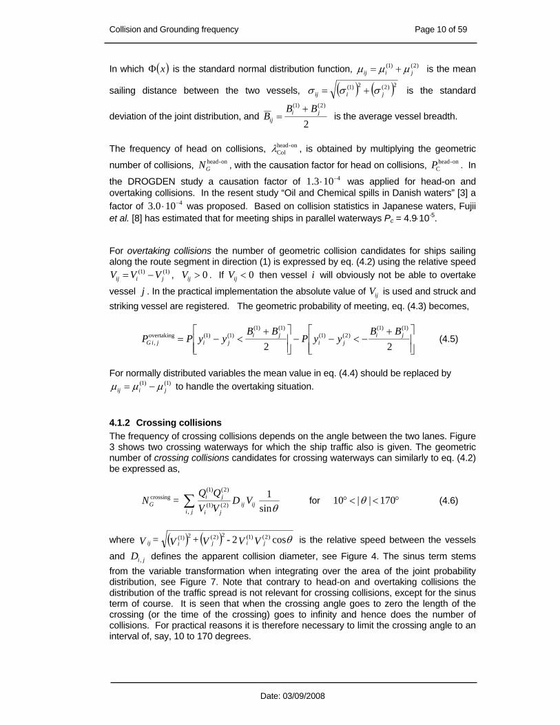
In which ( )xΦ is the standard normal distribution function, )2()1(jiij μμμ += is the mean
sailing distance between the two vessels, ( ) ( )2)2(2)1(jiij σσσ += is the standard
deviation of the joint distribution, and 2
)2()1(ji
ij
BBB
+= is the average vessel breadth.
The frequency of head on collisions, on-head
Colλ , is obtained by multiplying the geometric
number of collisions, on-headGN , with the causation factor for head on collisions, on-head
CP . In
the DROGDEN study a causation factor of 4103.1 −⋅ was applied for head-on and overtaking collisions. In the resent study “Oil and Chemical spills in Danish waters” [3] a factor of 4100.3 −⋅ was proposed. Based on collision statistics in Japanese waters, Fujii et al. [8] has estimated that for meeting ships in parallel waterways Pc = 4.9⋅10-5. For overtaking collisions the number of geometric collision candidates for ships sailing along the route segment in direction (1) is expressed by eq. (4.2) using the relative speed
)1()1(jiij VVV −= , 0>ijV . If 0<ijV then vessel i will obviously not be able to overtake
vessel j . In the practical implementation the absolute value of ijV is used and struck and striking vessel are registered. The geometric probability of meeting, eq. (4.3) becomes,
⎥⎥⎦
⎤
⎢⎢⎣
⎡ +−<−−
⎥⎥⎦
⎤
⎢⎢⎣
⎡ +<−=
22
)1()1()2()1(
)1()1()1()1(overtaking
,ji
jiji
jijiG
BByyP
BByyPP (4.5)
For normally distributed variables the mean value in eq. (4.4) should be replaced by
)1()1(jiij μμμ −= to handle the overtaking situation.
4.1.2 Crossing collisions The frequency of crossing collisions depends on the angle between the two lanes. Figure 3 shows two crossing waterways for which the ship traffic also is given. The geometric number of crossing collisions candidates for crossing waterways can similarly to eq. (4.2) be expressed as,
VDVVQQ
= Nji
ijijji
jiG ∑
,)2()1(
)2()1(crossing
sin1θ
for °<<° 170||10 θ (4.6)
where ( ) ( ) θcos2 )2()1()2( 2)1( 2 V V - V + V = V jijiij is the relative speed between the vessels
and jiD , defines the apparent collision diameter, see Figure 4. The sinus term stems from the variable transformation when integrating over the area of the joint probability distribution, see Figure 7. Note that contrary to head-on and overtaking collisions the distribution of the traffic spread is not relevant for crossing collisions, except for the sinus term of course. It is seen that when the crossing angle goes to zero the length of the crossing (or the time of the crossing) goes to infinity and hence does the number of collisions. For practical reasons it is therefore necessary to limit the crossing angle to an interval of, say, 10 to 170 degrees.

Collision and Grounding frequency Page 11 of 59
Date: 03/09/2008
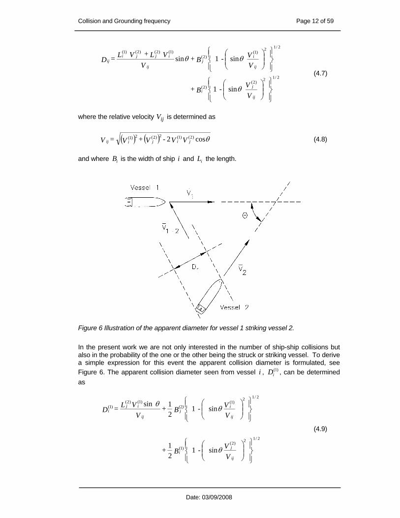
Figure 4 Definition of geometrical collision diameter Dij.
Figure 5 Calculation of the geometrical collision diameter ijD .
As mentioned ijD is the geometrical collision diameter illustrated in Figure 4. If it is assumed that the ships can be approximated by rectangular shapes, then it can be shown, see Figure 5, that:
Collision and Grounding frequency Page 12 of 59
Date: 03/09/2008
⎪⎭
⎪⎬⎫
⎪⎩
⎪⎨⎧
⎟⎟⎠
⎞⎜⎜⎝
⎛
⎪⎭
⎪⎬⎫
⎪⎩
⎪⎨⎧
⎟⎟⎠
⎞⎜⎜⎝
⎛
VV - B +
VV - B +
VV L + V L = D
ij
ji
ij
ij
ij
ijjiij
)2( 2 2/1
)2(
)1(2 2/1
)2()1()2()2()1(
sin1
sin1sin
θ
θθ
(4.7)
where the relative velocity ijV is determined as
( ) ( ) θcos2 )2()1()2( 2)1( 2 V V - V + V = V jijiij (4.8) and where iB is the width of ship i and iL the length.
Figure 6 Illustration of the apparent diameter for vessel 1 striking vessel 2.
In the present work we are not only interested in the number of ship-ship collisions but also in the probability of the one or the other being the struck or striking vessel. To derive a simple expression for this event the apparent collision diameter is formulated, see Figure 6. The apparent collision diameter seen from vessel i , )1(
iD , can be determined as
⎪⎭
⎪⎬⎫
⎪⎩
⎪⎨⎧
⎟⎟⎠
⎞⎜⎜⎝
⎛
⎪⎭
⎪⎬⎫
⎪⎩
⎪⎨⎧
⎟⎟⎠
⎞⎜⎜⎝
⎛
VV - B +
VV - B +
V V L = D
ij
ji
ij
i(2)j
ij
iji
)2( 2 2/1
)1(
)1(2 2/1
)1()2()1(
sin121
sin121sin
θ
θθ
(4.9)

Collision and Grounding frequency Page 13 of 59
Date: 03/09/2008
Similarly, for the case where vessel j in waterway 2 is striking vessel i in waterway 1 the apparent collision diameter is:
⎪⎭
⎪⎬⎫
⎪⎩
⎪⎨⎧
⎟⎟⎠
⎞⎜⎜⎝
⎛
⎪⎭
⎪⎬⎫
⎪⎩
⎪⎨⎧
⎟⎟⎠
⎞⎜⎜⎝
⎛
VV - B +
VV - B +
V V L = D
ij
ij
ij
ji
ij
jij
)1(2 2/1
)2(
)2( 2 2/1
)1()2()1(
)2(
sin121
sin121sin
θ
θθ
(3.10)
It is seen that the total collision diameter ijD is the sum of the two apparent collision diameters, i.e.: D + D = D (2)
j(1)iij
The probability of vessel i in waterway 1 striking vessel j in waterway 2 given a collision may then be determined as
[ ]ij
i
DDji P
)1(
= collision | vessel vessel → (4.12)
Similarly, the probability of vessel j in waterway 2 striking vessel i in waterway 1 is found as
[ ]DDij P
ij
j)2(
= collision | vessel vessel → (4.13)
The frequency, shipship−λ , of ship-ship collision per time unit is then determined as N P = jiGjiCshipship ,,.λ (4.14) Due to the fact that both of the involved two ships have the possibility of making aversive manoeuvres, the causation probability, CP , for ship-ship collision is smaller than the one given for grounding and collision against fixed objects, see Section 5.1. Based on collision statistics in Japanese waters, Fujii et al. [8] has estimated that for crossing ships Pc = 1.2⋅10-4 and for meeting ships in parallel waterways Pc = 4.9⋅10-5. Given the frequency of the (annual) number of collisions shipship−λ the probability of having a collision during time interval Δt can be estimated on the assumption of arrivals of the collisions as points in a Poisson process: 0for ][exp0.1]Collision[ →Δ≈Δ λλλ ship-shipship-shipship-ship tt - - = P Provided, of course, that the collision frequency of is time invariant.

Collision and Grounding frequency Page 14 of 59
Date: 03/09/2008
Figure 7 Basic layout of the simulated crossings with results presented in Figure 8 and Figure 9.
Figure 8 Comparison between simulated results assuming a Poisson distribution of ships in the two waterways and analytical results using Eq. (3.6)

Collision and Grounding frequency Page 15 of 59
Date: 03/09/2008
Figure 9 Simulated and analytical results for the probability of vessel 2 colliding with vessel 1 given a collision.
In order to verify the established analytical model and at the same time gain insight in the sensitivity of the number of collision candidates with respect to parameters such as crossing angles θ , ship dimensions, and ship speeds a program has been written which is based on time simulation. What has been considered is vessels of the same type in waterway 1 crossing the axis ξ, see Figure 7, as points in a Poisson process with intensity Q1 = 20000 vessels per year. The vessels in waterway 1 are assumed normally distributed over the width of the channel with μ = 100 m and σ = 45 m. Similar assumptions are made for vessels in waterway 2 crossing the axis ζ in Figure 7. Here Q2 = 50000 vessels per year and μ = 100 m and σ = 45 m. The vessels in the two waterways are moving with speed V1 and V2, respectively. A time history of +/- one hour of simulated vessels in waterway 1 is kept for matching against simulated vessels in waterway 2, i.e. t1 - 3600 s < t2 < 3600 s + t1. During the simulation it is calculated whether or not the two vessels are colliding. If they are observed to collide, it is further identified which of the vessels is the struck vessel and which is the striking vessel. Figure 8 shows the number of collision candidates during a period of forty years determined by time simulation and determined by the analytical expression Eq. (3.6) as functions of the angle θ between the two waterways.
4.1.3 Collision test cases This subsection describes the result of a series of selected test cases that were analysed by use of the GRISK program and by hand calculation. Only the number of collision candidates is calculated.

Collision and Grounding frequency Page 16 of 59
Date: 03/09/2008
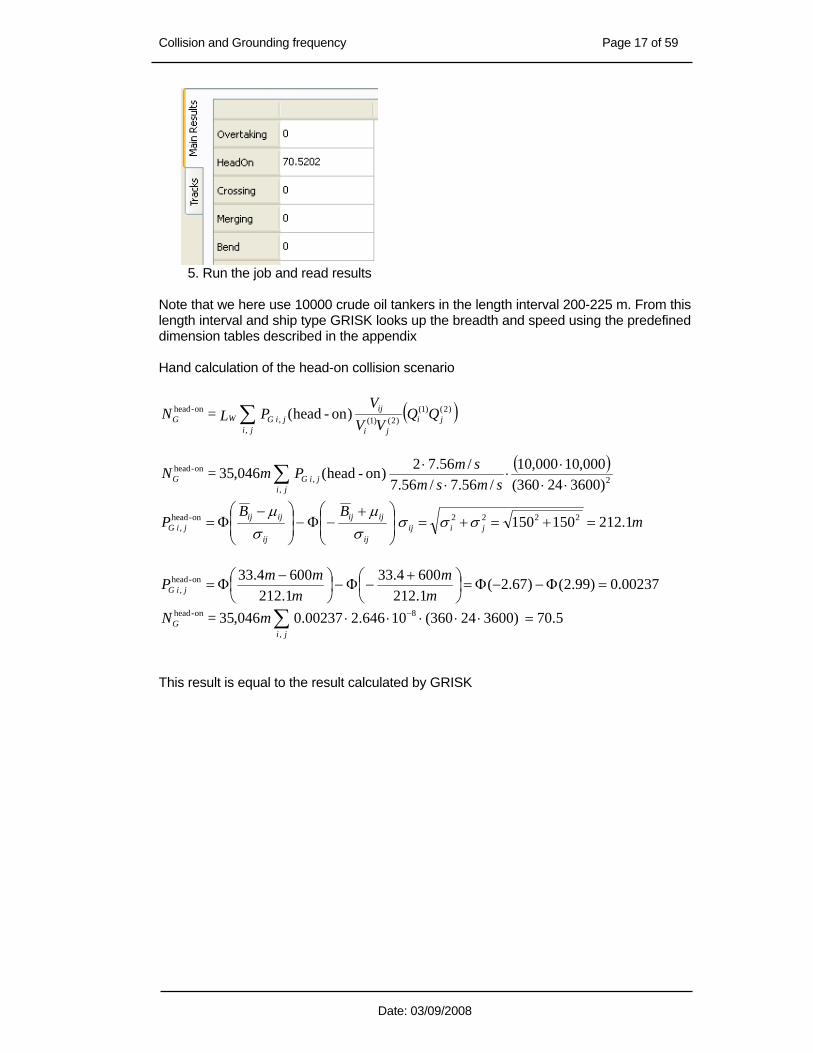
4.1.3.1 Test 1, Head on collision Test case 1 calculates the number of head on collisions per year. The scenario is: Length of leg 35,046 m Ships in each direction 10,000 Length of ships 214 m Breadth of ships 33.4 m Speed of ships 14.7 knots Traffic distribution Normal dist Mean position from leg 300 m Standard deviation 150 m Causation factors 1.0
To calculate this scenario in the BaSSy toolbox, GRISK, do the following steps:
1. Define leg 2. Define traffic distribution in each direction
3 .Define causation factors 4. define number of ships in each direction
Collision and Grounding frequency Page 17 of 59
Date: 03/09/2008
5. Run the job and read results Note that we here use 10000 crude oil tankers in the length interval 200-225 m. From this length interval and ship type GRISK looks up the breadth and speed using the predefined dimension tables described in the appendix Hand calculation of the head-on collision scenario
( ) QQVV
V P L = N
jiji
ji
ijjiGWG ∑
,
)2()1()2()1(,
on-head )on-head(
( )
smsmsm P m = N
jijiGG ∑ ⋅⋅
⋅⋅
⋅⋅
,2,
on-head
)360024360(000,10000,10
/56.7/56.7/56.72)on-head(046,35
⎟⎟⎠
⎞⎜⎜⎝
⎛ +−Φ−⎟
⎟⎠
⎞⎜⎜⎝
⎛ −Φ=
ij
ijij
ij
ijijjiG
BBP
σμ
σμon-head
, mjiij 1.212150150 2222 =+=+= σσσ
00237.0)99.2()67.2(1.2126004.33
1.2126004.33on-head
, =Φ−−Φ=⎟⎠⎞
⎜⎝⎛ +−Φ−⎟
⎠⎞
⎜⎝⎛ −
Φ=m
mm
mmP jiG
5.70)360024360(10646.200237.0046,35,
8on-head =⋅⋅⋅⋅⋅∑ − m = Nji
G
This result is equal to the result calculated by GRISK

Collision and Grounding frequency Page 18 of 59
Date: 03/09/2008
4.1.3.2 Test 2: Overtaking collision Calculates the number of collisions per year on a leg where ships sail in the same direction but at different speeds. The scenario is: Length of leg 35,046 m Number of ship 1 10,000 Length of ship 1 214 m Breadth of ship 1 33.2 m Speed of ship 1 14.7 knots Number of ship 2 10,000 Length of ship 2 162 m Breadth of ship 2 25.0 m Speed of ship 2 18.9 knots Mean position from leg 300 m Standard deviation 150 m Causation factors 1.0
To calculate this scenario in GRISK, do the following steps:
1. Define leg 2. Define traffic distribution in each direction
3 .Define causation factors 4. define two number of ships

Collision and Grounding frequency Page 19 of 59
Date: 03/09/2008
5. Run the job and read results Hand calculation of the head-on collision scenario This only difference to the head on collision calculation is the sign of the two speeds.
( ) QQVV
V P L = N
jiji
ji
ijjiGWG ∑
,
)2()1()2()1(,
overtaking )on-head(
smsm
sm P m = Nji
jiGG ∑ ⋅⋅⋅
⋅⋅
−
,2,
overtaking
)360024360(000,10000,10
/56.7/72.9/)56.772.9()on-head(046,35
⎟⎟⎠
⎞⎜⎜⎝
⎛ +−Φ−⎟
⎟⎠
⎞⎜⎜⎝
⎛ −Φ=
ij
ijij
ij
ijijjiG
BBP
σμ
σμovertaking
,
mjiij 1.212150150 2222 =+=+= σσσ
1095.0)138.0()138.0(1.212
02/)2539.33(1.212
02/)2539.33(overtaking,
=−Φ−Φ=
=⎟⎠⎞
⎜⎝⎛ ++−Φ−⎟
⎠⎞
⎜⎝⎛ −+
Φ=m
mmm
mmP jiG
5.362)360024360(10037.31095.0046,35
,
9overtaking =⋅⋅⋅⋅⋅∑ − m = Nji
G
This result is equal to the result calculated by GRISK.

Collision and Grounding frequency Page 20 of 59
Date: 03/09/2008
4.1.3.3 Test 3: Crossing collision Test case 3 calculates the number of crossing collisions per year. The scenario is: Ships North going 10,000 Ships East going 10,000 Length of ships 200 m Breadth of ships 33.4 m Speed of ships 14.7 knots Angle between legs 88.8 deg Causation factors 1.0
In GRISK this scenario is defined as follows:
1. Define the legs 4. Define number of ships on each leg and the
causation factors
4. Define how much traffic sails from one leg to the others
Run the program and read the results
Hand calculation of the crossing collisions scenario
Collision and Grounding frequency Page 21 of 59
Date: 03/09/2008
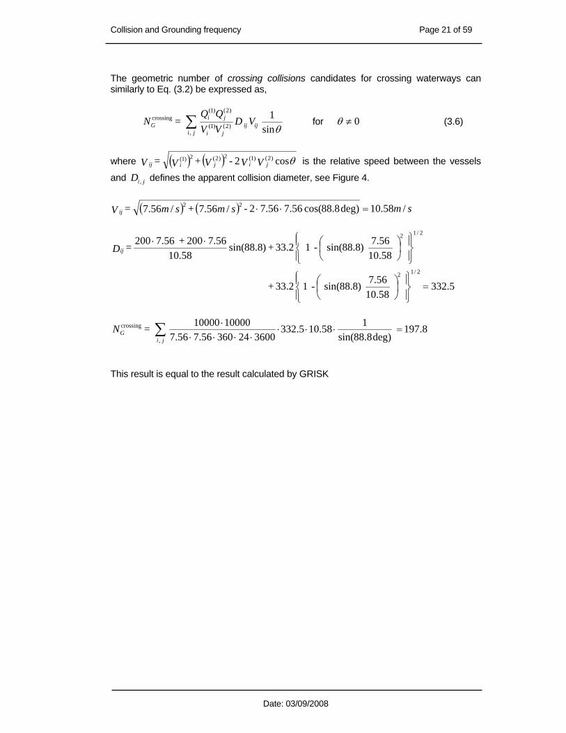
The geometric number of crossing collisions candidates for crossing waterways can similarly to Eq. (3.2) be expressed as,
VDVVQQ
= Nji
ijijji
jiG ∑
,)2()1(
)2()1(crossing
sin1θ
for 0≠θ (3.6)
where ( ) ( ) θcos2 )2()1()2( 2)1( 2 V V - V + V = V jijiij is the relative speed between the vessels
and jiD , defines the apparent collision diameter, see Figure 4.
( ) ( ) sm - sm + sm = V ij /58.10deg)8.88cos(56.756.72/56.7/56.7 22 =⋅⋅
5.33258.1056.7)8.88sin(12.33
58.1056.7)8.88sin(12.33)8.88sin(
58.1056.720056.7200
2 2/1
2 2/1
=⎪⎭
⎪⎬⎫
⎪⎩
⎪⎨⎧
⎟⎠⎞
⎜⎝⎛
⎪⎭
⎪⎬⎫
⎪⎩
⎪⎨⎧
⎟⎠⎞
⎜⎝⎛⋅⋅
- +
- + + = Dij
8.197deg)8.88sin(
158.105.33236002436056.756.7
1000010000,
crossing =⋅⋅⋅⋅⋅⋅⋅
⋅∑ = Nji
G
This result is equal to the result calculated by GRISK

Collision and Grounding frequency Page 22 of 59
Date: 03/09/2008
4.1.3.4 Test 4: Merging collision Collision due to merging traffic is calculated as crossing collisions
Merging traffic
4.2 Probability of grounding Following Pedersen [25], the grounding scenarios may broadly be divided into four main categories, see Figure 10:
I. Ships following the ordinary direct route at normal speed. Accidents in this category are mainly due to human error, but may include ships subject to unexpected problems with the propulsion/steering system that occur in the vicinity of the fixed marine structure or the ground.
II. Ships that failed to change course at a given turning point near the obstacle. III. Ships taking evasive actions near the obstacle and consequently run aground or
collide with the object. IV. All other track patterns than Cat. I, II and III, for example ships completely out of
course due to loss of propulsion. Figure 10 shows observed grounding locations in a part of the Great Belt in Denmark over a 15-year-period. It is seen that most of the grounding events belong to category I and II but there are also category III and IV groundings which seem to be randomly scattered over the area. In formulating a theoretical model for the grounding scenario it is expedient to divide the grounding scenario into powered groundings and drifting groundings. Such division eases not only the frequency assessment but also the pursuing consequence assessment.

Collision and Grounding frequency Page 23 of 59
Date: 03/09/2008
Figure 10 Observed grounding events over a 15-year-period in a Danish Strait, from [25].
In the following, expressions are presented for predicting the expected annual number of grounding events of category I and II accidents. The probability of category III and IV grounding events are today normally found by modification of the traffic distribution along the route. In the present work drifting ships (category IV) are modelled by assuming a drifting direction according to a user specified wind rose. Evasive manoeuvres (category III are not explicitly dealt with in the present version. We revert to these issues later.

Collision and Grounding frequency Page 24 of 59
Date: 03/09/2008
Ships in category I and II, following an ordinary route, are distributed over a transverse section of the waterway with some probability density function, )(zfi , where index i refers to a ship class and z is the transverse coordinate, see Figure 11. The shape of if is a strong function of the considered waterway so a major challenge of the present approach is to define rationally )(zfi along a given route. Given if the number of candidates of grounding events can be calculated as an integral of if over the width,
minz to maxz , of the obstacle. The hatched area in Figure 11 illustrates this. Most of these candidates will be aware of the danger and take the necessary aversive actions before they hit the obstacle. However, a fraction, cP , of the candidates will fail to avoid the obstacle, due to for example human and technical errors. The fraction cP is normally referred to as the “causation probability”, and it will be shown later how it can be estimated. Groundings that are caused by a meeting situations where ships may feel forced to give way, which then subsequent may result in grounding, has not been considered. Such a model requires much more advanced modelling than what is implemented at the present stage. Neither have groundings that are caused by a “rudder stuck” failure. In this case the rudder may either go the extreme starboard/port side or it will get stuck in a central position and cause the vessel either to turn in circles or to follow its path. The model requires more data information before it will be implemented.
Figure 11 Illustration of model for predicting the expected number of grounding events or collisions with fixed objects on a given ship route, from [25].
4.2.1 Powered grounding According to the model described above, the expected number of grounding events in Category I and II can be calculated as
∑ ∫=i class, Ship
max
min, )(
z
ziiicI dzzfQPN (4.15)
∑ ∫−=i class, Ship
,
max
min
)()/exp(z
ziiiicII dzzfadQPN (4.16)

Collision and Grounding frequency Page 25 of 59
Date: 03/09/2008
where the following notation has been used:
ia Average distance between position checks by the navigator.
d Distance from the obstacle to the bend in the navigation route varying with the lateral position, s, of the ship.
i Index for ship class, categorised after vessel type and dead weight or length.
)(zfi Probability density function for the ship traffic
IN Expected number of category I grounding events per year.
IIN Expected number of category II grounding events per year.
icP , Causation probability, i.e. ratio between ships grounding and ships on a grounding course.
iQ Number of ships in class i passing a cross section of the route per year.
z Coordinate in the direction perpendicular to the route.
minz , maxz Transverse coordinates for an obstacle.
In the above it is assumed that the event of checking the position of the ship can be described as a Poisson process. Thus, the factor )/exp( iad− represents the probability of the navigator not checking the position from the bend to the obstacle. The average distance between position checks is conveniently expressed in terms of the expected value of the time between position checks, λ , (approximately equal to 3 minutes) whereby the factor )/exp( iad− becomes a function of the ship speed, Vai λ= . Eq. (4.16) is only correct for the case when the ground is orthogonal to the sailing route, which rarely is the case. In the event of the ground not being perpendicular to the sailing direction, but inclined so that the distance d from the bend to the ground may be expressed as bazd += . In the event that the two traffic spread distributions follow a normal distribution then Eq. (4.16) can be simplified to
∑⎥⎥⎦
⎤
⎢⎢⎣
⎡
⎪⎭
⎪⎬⎫
⎪⎩
⎪⎨⎧
−⎟⎟⎠
⎞⎜⎜⎝
⎛ +Φ⎟
⎟⎠
⎞⎜⎜⎝
⎛ −=
i class, Ship
max
min
2
22
22
, 122
2exp21
z
z
iicII VaVz
VVbaQPN
σλσλ
λλσ
(4.17)
For other type of distributions, especially for mixed distributions, it is not a straight forward task to formulate a closed form solution to the number of grounding candidates. For such distributions the integral can be effectively solved by solving part of the integral analytical and then performing a numerical integration over the remaining variables. With the formulation above the expected number of annual grounding events becomes a function of traffic distributions, bottom topology, route layout etc. It is seen from Eq. (4.15), (4.16) and (4.17) that another important parameter is the causation factor, cP , determining how large a fraction of the accident candidates actually run aground or hit the obstacle. Chapter 5 gives a thorough presentation of the causation factor. Often the causation probability is selected to be in the vicinity to 4102 −⋅=cP .

Collision and Grounding frequency Page 26 of 59
Date: 03/09/2008
The calculated expected number of yearly (powered) grounding events, IIIg NNN += , can be considered as the intensity in a Poisson process. The probability of no grounding events in one year is then [ ] )exp(1 gNGroundingP −−= (4.18)
4.2.2 Drifting grounding The probability of category III (evasive manoeuvres) and category IV (drifting ships) grounding events are today typically found by modification of the traffic distribution along the route. Combining a 98% Gaussian distribution and a 2% uniform distribution performs the modification of the traffic distribution; see e.g. Gluver and Olsen [12] or Karlson et al. [19]. The value of 2% is based on engineering judgement and the results are dependent on the value especially in narrow restricted waters. Although this approach is very fast and easy to implement, it is considered to be too coarse a model that does not properly account for the physical effects that governs the drifting problem. In the section the implemented drifting model is defined. The two main causes for a ship to be not under command are rudder stuck and blackout of the main engine. Rudder stuck will not be dealt with in this study. Most ships experiences of the order of one black out of the main engine per year. The number of any blackout for a given ship will typically lie in the interval from 0.1 to 2 blackouts per year. The actual frequency of blackouts depends on the degree of redundancy and the general maintenance level of the ships. Ferries and ro/ro vessels generally have a high degree of built-in redundancy into the engine room (2 to 4 propulsion units) and hence they have a low frequency of blackouts. For many other single propulsion unit ships the frequency of blackouts are higher. In the present study the following blackout frequencies are selected as base values:
Vessel type Annual frequency Hourly frequency Passenger / Ro-Ro 0.1 y-1 1.15·10-5 h-1
Other vessels 0.75 y-1 8.56·10-5 h-1 A blackout may be caused by contaminated fuel, internal fault in the main engine, or failure of the electrical system. The seriousness of the incident depends on the location at which the blackout occurs, the wind direction, wind speed, and of course the duration of the blackout (that is the drifting time). If a high degree of redundancy has been built into the engine room then the command over vessel may be regained in relative short time. In other situations, the drifting time may be of order of hours. The drifting ship will drift side ways and it will drift (approximately) in the direction of the wind. The drifting scenario may be remediated either by repairing the problem, by anchoring the vessel or by calling a tug boat. Failure of propulsion machinery may occur at any location along the waterway. Assuming that blackouts occur as points in a Poisson process then the probability of having a blackout along a leg segment of length segmentL is:
( ) ⎟⎟⎠
⎞⎜⎜⎝
⎛−−=
vessel
segmentblackoutsegmentblackout exp1
vL
LP λ
Collision and Grounding frequency Page 27 of 59
Date: 03/09/2008
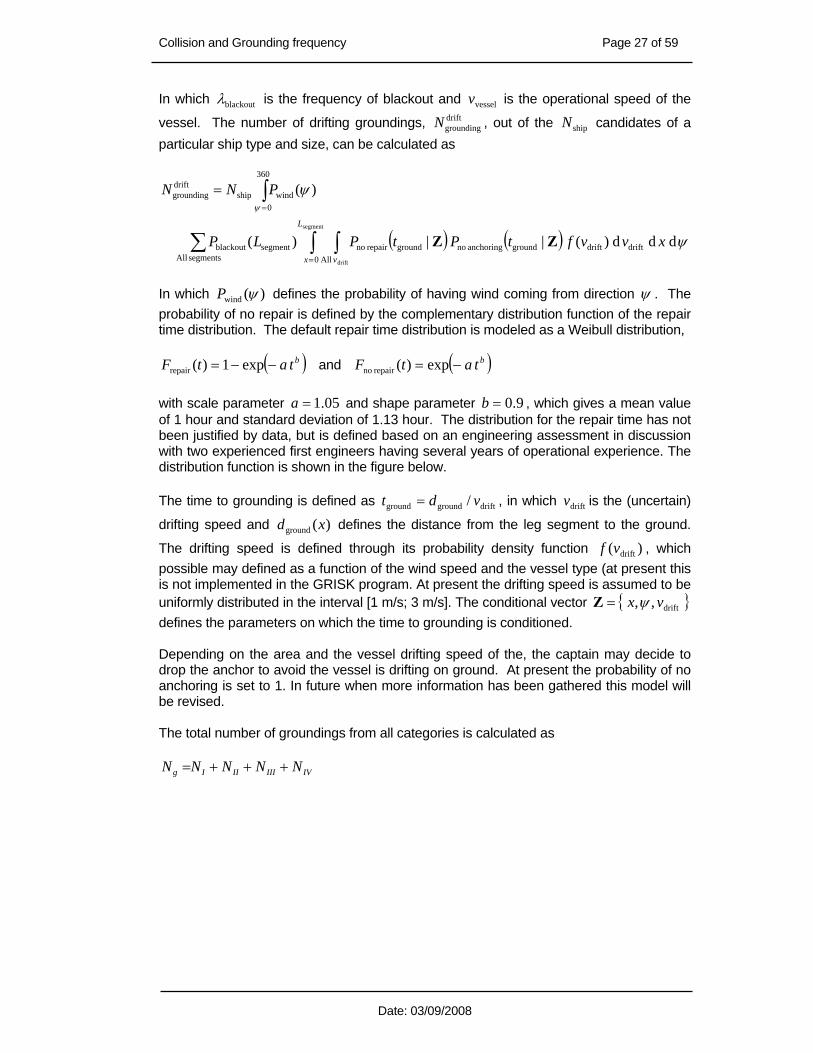
In which blackoutλ is the frequency of blackout and vesselv is the operational speed of the
vessel. The number of drifting groundings, driftgroundingN , out of the shipN candidates of a
particular ship type and size, can be calculated as
( ) ( )∫ ∫∑
∫
=
=
=
segment
drift0driftdriftgroundanchoring nogroundrepair no
Allsegments Allsegmentblackout
360
0windship
driftgrounding
ddd)(||)(
)(
L
x v
xvvftPtPLP
PNN
ψ
ψψ
ΖΖ
In which )(wind ψP defines the probability of having wind coming from direction ψ . The probability of no repair is defined by the complementary distribution function of the repair time distribution. The default repair time distribution is modeled as a Weibull distribution,
( )btatF −−= exp1)(repair and ( )btatF −= exp)(repair no with scale parameter 05.1=a and shape parameter 9.0=b , which gives a mean value of 1 hour and standard deviation of 1.13 hour. The distribution for the repair time has not been justified by data, but is defined based on an engineering assessment in discussion with two experienced first engineers having several years of operational experience. The distribution function is shown in the figure below. The time to grounding is defined as driftgroundground / vdt = , in which driftv is the (uncertain)
drifting speed and )(ground xd defines the distance from the leg segment to the ground.
The drifting speed is defined through its probability density function )( driftvf , which possible may defined as a function of the wind speed and the vessel type (at present this is not implemented in the GRISK program. At present the drifting speed is assumed to be uniformly distributed in the interval [1 m/s; 3 m/s]. The conditional vector { }drift,, vx ψ=Ζ defines the parameters on which the time to grounding is conditioned. Depending on the area and the vessel drifting speed of the, the captain may decide to drop the anchor to avoid the vessel is drifting on ground. At present the probability of no anchoring is set to 1. In future when more information has been gathered this model will be revised. The total number of groundings from all categories is calculated as
IVIIIIIIg NNNNN +++=

Collision and Grounding frequency Page 28 of 59
Date: 03/09/2008
4.3 Assessing the traffic spread across the route With access to AIS data it is a relative straight forward task to assess the probability distribution of the traffic spread across the route as well as the number and the composition of the vessel traffic. When such data are not available it is a quite involved task to identify the needed data. Only little guidance has been found in literature on the geometric distribution of the traffic. Typically a normal distribution is selected. Gluver and Olsen [12] proposed to apply a standard deviation equal to ship length. Alternatively the standard deviation of the Gaussian distribution can be selected to be proportional to the vessel breadth, B65,3=σ . This choice corresponds to a 96% probability of the vessel being within B5.7± of the planned route, which again reflects the zone within which the navigator of the vessel identifies safe operation. In the study by Karlson et al. [19] the standard deviation of the Gaussian distribution was chosen to 40% of the navigational channel.
4.4 Calculation procedure for estimating the collision frequency Based on the mathematical models for estimating the collision grounding frequencies described in the previous sections a computer program has been written for calculation of grounding and collision frequencies in specific waterways where the ship traffic distribution is known. As earlier described, the idea behind the procedure is that vessels are operating on specific route. The traffic routes are built of a series of waypoints that are connected by legs. On each leg the number of vessels as a function of size and type and their overall spreading are defined. Each leg may be connected to zero, one or more other segments at its end points. In principle three different types of collisions can occur. One type of collision is head-on induced collisions due to two way traffic in the straight waterway segments or overtaking taking collisions as shown in Figure 2. As seen from Eq. (4.4) then the traffic distributions are importance in this case. Another type of collision occurs at bends where only two straight route segments intersect, see Figure 12. At such an intersection a ship can become a collision candidate if the course is not changed at the intersection. This probability of omission P0 is taken as 0.01.
Figure 12 Intersection between two straight waterway segments.
Collision and Grounding frequency Page 29 of 59
Date: 03/09/2008
Finally, when more than two legs meet at a waypoint the model calculates the probability for crossing collisions, as indicated in Figure 3. Dependent on how the vessel traffic on the legs meets each other, the scenario will be characterized either as either a crossing collision, a merging collision, or a bend collision. For each leg the identified number of collision candidates related to head-on, bends, and crossings is calculated for each vessel type and is subsequent multiplied by a causation factor. The following causation factors inspired by Fujii et al. [8]:
P[head on] = 4.9⋅10-5 P[bend] = 1.3⋅10-4 P[crossing] = 1.3⋅10-4
These values for the causation factor are typical values for well regulated ship traffic in Japan. The causation factor will be a function of visibility, darkness, current and wind in the actual geographical area. All these factors suggest that larger values should be used around the Nordic countries. However, Fujii has also observed that passenger ferries have smaller collision probabilities than ordinary merchant vessels. This is due to the navigator awareness of the area and the fact that there are two navigator onboard passenger ferries. The following chapter discusses the assessment of the causation probability in more detail. The causation factors suggested used in the present study are presented in section 5.3.
4.5 Combined causation factor jiCP , The causation probability, jiCP , , represents the probability that none of the two officers on watch on the two vessels manage to react in time and avoid the collision. This implies that the conditions present on both vessels are of importance in the determination of the magnitude of the causation joint factor. This concept is illustrated by a Bayesian network model in a subsequent section. Different conditions may be present that lead to higher (or lower) safety standards compared to the average ship. This could for instance be the presence of a pilot, improved bridge layout and navigational equipment, or the presence of two navigators as is the case on most passenger ferries. The presence of such safety increasing conditions will imply that the joint causation factor, jiCP , , for the two vessels will decrease. In the study “Oil and Chemical Spills is Danish waters” it was proposed to compile the joint causation factor as
jCiCjiC PPP ×=, (3.15) This is a justifiable pragmatic approach that assures a balance between failures of the navigational watch keeping on the two vessels.
5. CAUSATION PROBABILITY This chapter presents a comprehensive collection of causation probabilities that have been proposed in literature. Further, a risk model that may be used for evaluating the causation probability is presented. Inadequacies of a frequently cited risk model are discussed and instead we propose to apply Bayesian Networks. A Bayesian Network for obtaining the causation factor for ship-ship collision is established, and the results are compared to available statistics, where good agreement was found.

Collision and Grounding frequency Page 30 of 59
Date: 03/09/2008
5.1 Causation probabilities from literature Larsen [20] performed a comprehensive study on defined causation probabilities in his study of ship collisions with bridges. Although the study primarily addresses ship-bridge collisions, Larsen [20] also presented available causation probabilities for ship grounding and ship-ship collisions. The table below represents an organised table of his review, which further has been extended with some results not given in [20]. References to these are given in the present note. The full references to the authors identified by Larsen [20], will not be given here but may be found in section 5.3 of reference [20].
Vessel grounding Location Pc
[×10-4]
Comment Reference:
see [20] for ref.
Japanese Straits [1.0; 6.3] Collisions and grounding Fujii
Japanese Straits 1.58 Fujii & Mizuki [9]
Japanese Straits [0.8; 4.3] Matsui
Dover Strait 1.55 No traffic separation MacDuff [21]
Dover Strait 1.41 With traffic separation MacDuff [21]
Strait of Gibraltar 2.2 COWIconsult
Øresund, Denmark 2.0 Karlson et al. [19]
Ship-ship collisions Location Pc
[×10-4]
Comment Reference:
see [20] for ref.
Dover Strait 5.18 Head-on, no traffic separation
MacDuff [21]
Dover Strait 3.15 Head-on, with traffic separation
MacDuff [21]
Øresund, Denmark 0.27 Head on Karlson et al. [19]
Japanese Straits 0.49 Head on Fujii & Mizuki [9]
Japanese Straits 1.23 Crossings Fujii & Mizuki [9]
Dover Strait 1.11 Crossings, no traffic separation
MacDuff [21]
Dover Strait 0.95 Crossings, with traffic separation
MacDuff [21]
Strait of Gibraltar 1.2 COWIconsult
Japanese Straits 1.10 Overtaking Fujii & Mizuki [9]
Great Belt, Denmark 1.30 At bends in lanes Pedersen et al. [24]
Danish waters 3.0 Head-on and overtaking
Crossings also?
COWIconsult Oil and Chemical Spills, 2007

Collision and Grounding frequency Page 31 of 59
Date: 03/09/2008
Ship-bridge collisions
Location Pc
[×10-4]
Comment Reference:
see [20] for ref.
Great Belt 0.4 Traffic regulations, marking of route, detectability
Larsen
Great Belt East and West Bridge
1.1 Having pilot on board COWIconsult
Great Belt East and West Bridge
3.2 Without pilot on board COWIconsult
Tasman Bridge [0.7; 1.0] Visibility, env. conditions, human error, mechanical failure, traffic intensity
Maunsell and Partners
Sunshine Skyway Bridge, Florida
0.5 Traffic density, use of pilots, traffic restrictions
COWIconsult
Annacis Island Bridge, Fraser River, British Columbia
3.6 CBA-Buckland and Taylor
Sunshine Skyway Bridge, Florida
1.3 Ships only Knott et al.
Sunshine Skyway Bridge, Florida
2.0 Barges only Knott et al.
Francis Scott Key Bridge 1.0 Ships only Knott et al.
Francis Scott Key Bridge 2.0 Barges only Knott et al.
Wm Preston Lane, Jr. Men. Bridge, Maryland
1.0 Ships only Knott et al.
Wm Preston Lane, Jr. Men. Bridge, Maryland
2.0 Barges only Knott et al.
Chesapeake Bay Bridges and Tunnels, Virginia
0.7 Knott et al.
Dames Point Bridge, Florida 1.3 Ships only Knott et al.
Dames Point Bridge, Florida 4.1 Barges only Knott et al.
Vicksburg Bridge, Mississippi River
5.4 Modjeski & Masters
Huey P. Long Bridge, Mississippi River
2.5 Modjeski & Masters
Greater New Orleans Bridge, Mississippi River
1.3 Modjeski & Masters
Strait of Gibraltar 0.6 Improved traffic safety COWIconsult
Japanese Straits 1.86 Fujii & Mizuki [9] The values of the causation probabilities by Fujii and Mizuki [9] given in the tables above are mean values. Fujii and Mizuki [9] have given the following ranges:

Collision and Grounding frequency Page 32 of 59
Date: 03/09/2008
log Pc = -4.31 ± 0.35 for head-on collisions
log Pc = -3.96 ± 0.36 for collisions in overtaking log Pc = -3.89 ± 0.34 for collisions in crossing log Pc = -3.80 ± 0.26 for grounding log Pc = -3.73 ± 0.36 for collisions with objects
Further, Fujii and Mizuki [9] states that the above given causation probabilities are obtained for a frequency of visibility less than 1 km that is equal to 263 hours pr. year (i.e. 3%). They further state that the influence of low visibility on the causation probability is approximately proportional to the inverse of the visibility. Finally, they suggest to multiply the above given causation probabilities with a factor of 2 if the frequency of visibility less than 1 km. is in the range of 3% to 10%, and a factor of 8 if it is in the range of 10% to 30%.
5.2 Risk model for obtaining the causation probability It is virtually impossible to formulate a full risk analysis that properly takes all relevant aspects into account. The modelling should, however, account for a subset as large as possible of the potential error mechanisms. This section describes the traditional risk analytical approach for obtaining the causation probability. We discuss the drawbacks of the traditional formulation and suggest applying Bayesian Network. The subsequent Chapter 6 describes aspects that should be considered in the modelling.
Figure 13 Fault tree for causation probability Pc for collision against fixed object.

Collision and Grounding frequency Page 33 of 59
Date: 03/09/2008
5.2.1 Traditional approach The traditional approach for calculation of Pc (i.e. analysing the cause leading to human inaction or external failures) is to formulate a fault tree or an event tree analysis, see Haugen [13], as shown in Figure 13. From this fault tree it is found that the causation probability Pc can be expressed as ( ) 211 CCAAC XXXXP −+= where XA is the probability of human failure XC1 is the probability of radar failure, which will depend on vessel size, age,
nationality, etc. XC2 is the fraction of the year with low visibility. By application of such fault tree analyses for estimation of the causation probability, it is possible to examine the beneficial effect of new bridge procedures, of having a pilot on board, or of introducing a VTS system in certain geographical areas. Olsen et al. [22] studied the effect of a VTS system by an event tree analysis, see Section 6.2.1. When inspecting the above fault tree it is questionable whether the modelling actually captures any of the important failure mechanism relevant for the considered critical situation. Factors that relate to navigational complications are not included in the analysis, although these are of importance for the relevant set of human errors. Moreover, it is seen that human failure contributes with 75% (2.6⋅10-4) to the causation probability. The dominance of the human failure is in agreement with observations. However, the “Asleep” node is the dominant contributor (2.0⋅10-4) and it accounts for 60% of the causation probability. Although the dominating cause may be attributed to human errors this does not seem to be correct as high vigilance is expected in confined navigational areas. An important concern of the fault tree modelling is that the human factor model does not capture the relevant tasks that must be considered in the considered critical situation.
5.2.2 Using Bayesian Networks Most practical risk analysis problems are characterised by a large set of interrelated uncertain quantities and alternatives. Within the conventional risk analysis different methods such as fault tree analysis and event tree analysis have been developed to address these problems. A fault tree analysis seeks the causes of a given event, and an event tree analysis seeks the consequences of a given event. The two analysis techniques are supplementary methods, and when applied correctly the formulated model may reveal the entire probability structure of the model. Both fault tree analysis and event tree analysis – applied separately and combined – have in the past with success been used in the evaluation of the risk of various hazardous activities. Unfortunately, both fault tree and event tree analyses do have their drawbacks. Firstly, it is difficult to include conditional dependencies and mutually exclusive events in a fault tree analysis (a conditional dependency is, for example, the dependence of the visibility on the weather; mutually exclusive events are, for example, good weather and storm). If conditional dependencies and mutually exclusive events are included in a fault tree analysis the implementation and the pursuing analysis must be performed with utmost care. Secondly, the size of an event tree increases exponentially in the number of variables. Thirdly, if the analysis should capture the primary failure mechanism, the global model, which is combined fault trees and event trees, generally becomes so big that it is virtually impossible for third parties (and sometimes even for first parties) to validate the model.

Collision and Grounding frequency Page 34 of 59
Date: 03/09/2008
Here we advocate for using Bayesian Networks as the risk modelling and analysis tool. A Bayesian Network is a graphical representation of uncertain quantities (and decisions) that explicitly reveals the probabilistic dependence between the set of variables and the flow of information in the model. A Bayesian Network is designed as a knowledge representation of the considered problem and may therefore be considered as the proper vehicle to bridge the gap between analysis and formulation.

Collision and Grounding frequency Page 35 of 59
Date: 03/09/2008
Figure 14 Example for Bayesian Network for a navigating officer reacts in the event of being on collision course with an object, from Friis Hansen and Pedersen [10].
Speed reducti
Weather Radar status
Day lightVisibility
Object type
Visual dist.
Radar dist.
Obj. rel. speed
Visual time
Radar time
Vessel speed Traffic intensit
Maneuv. timeTime for visual Time for radar
Other alarms OOW training
Stress level
Bridge
OOW Task
Alarm transfer
Looking freqRadar freqOOW visual
OOW radar
OOW acts
Collision and Grounding frequency Page 36 of 59
Date: 03/09/2008
A Bayesian Network is a network with directed arcs and no cycles. The nodes (to which the arcs point) represent random variables and decisions. Arcs into random variables indicate probabilistic dependence, while arcs into decisions specify the information available at the time of the decision. As an example, one node in the network may represent the weather, whereas another may represent the visibility. An arc from weather to visibility indicates that visibility is conditionally dependent on weather; see Figure 14. The diagram is compact and intuitive, emphasising the relationship among the variables, and yet it represents a complete probabilistic description of the problem. For example, it is easy to convert any event tree or fault tree into a Bayesian Network. Conversely, it may not always be an easy task to convert a Bayesian Network into a combined fault tree and event tree, although theoretically possible. A drawback of Bayesian Network is that they require the state space of the random variables (the nodes) to be defined as discrete states. In our above-mentioned example of weather and visibility, the state space of weather may easily be discretised into states as good weather, storm, etc., whereas the state for visibility more naturally would have been defined as a continuous state space. The Bayesian Network modelling does, unfortunately, require the state space of visibility to be discretised in ranges as for example, 0 to 1 km, 1 to 2 km, etc. Although this is mentioned as a drawback, neither fault trees nor event trees offer any better alternatives. A consequence of the discretisation is partly that the result of the Bayesian Network may be sensitive to the selected discretisation, and partly that the calculations involved in the evaluation of the Bayesian Network grow almost exponentially in the number of states of the nodes. The latter is a consequence of Bayesian Networks encodes the entire probabilistic structure of the problem. A focus on the causal relationship among the variables most effectively does the building of a Bayesian Network. This implies that a Bayesian Network becomes a reasonably realistic model of the problem domain, which is useful when we try to get an understanding about a problem domain. In addition, knowledge of causal relationships allows us to make predictions in the presence of interventions. Last, but not least, the model building through causal relationship makes it much easier to validate and convey the model to third parties. We will not give any details here on how Bayesian Networks are analysed. Instead reference is left to Jensen [18] and Pearl [23]. The Bayesian Network described above is taken from Friis Hansen and Pedersen [10] where a comparative risk evaluation of traditional watch keeping and one-watch keeping has taken pace. The results of the modelling were compared to observations, and good agreement was obtained. Here we extend the modelling to also cover ship-ship collisions.
5.2.3 Bayesian Network for ship-ship collisions The network for predicting the causation factor for ship-ship collisions is rooted in the network shown in Figure 14. The Bayesian Network was extended to model two ships, i.e. ship-ship collision situations. The network used for this analysis is presented as Figure 15. It is seen that this Bayesian Network take into account the correlation between the two vessels, that is, they have to detect each other under the same conditions. Although the network appears complicated, the elements from the basic network in Figure 14 are recognised. It is noted that the to more isolated groups in the lower part of the network models the behaviour on the two bridges, whereas the central group in the upper part of the figure models the two vessel that the two vessels has to be detected by each other.

Collision and Grounding frequency Page 37 of 59
Date: 03/09/2008
Figure 15 Bayesian Network model for ship-ship collisions accounting for the correlation between the two vessels.
Speed red B
Weather
Radar status B
Day light
Visibility
Visual dist. B
Radar dist. B
Visual time B
Radar time B
Traffic intensit Maneuv. time
Time for visual Time for radar
Alarms B OOW train B
Stress B
Bridge B
OOW Task B
Alarm trf B
Look freq B Radar freq BOOW vis B OOW radar B
OOW B actsOOW A acts
OOW radar A OOW vis ARadar freq A Look freq A
Alarm trf A
OOW Task A
Bridge A
Stress A
OOW train A Alarms A
Time for radar Time for visual
Maneuv. time
Radar time A
Visual time A
Radar dist. A
Visual dist. A
Radar status
Speed red A
Vessel AVessel B
Speed A Speed B
Rel. Speed
Collision

Collision and Grounding frequency Page 38 of 59
Date: 03/09/2008
Table 1 shows the calculated causation factors for all the combinations of meetings between large vessels with conventional bridge layout and vessels equipped for sole look-out. It is seen that the calculated causation factor for meetings between conventional vessels is found to be, [10], Pc = 9.00⋅10-5. This value can be compared with observed causation probabilities determined from large data sets published by Fujii et al. [9]. These observed values are given in Table 2. In Table 3 the different headings have been weighed to obtain one global causation factor. The result is that the observations indicate that the causation factor is close to Pc = 8.41⋅10-5 That is a factor which is very close to the causation factor Pc = 9.00 10-5 calculated by the Bayesian Network procedure for conventional vessels operating in geographical areas where the frequency of visibility less than 1 km is 3%. The modelling illustrates that it indeed is possible to establish a realistic modelling of the causation probability.
Table 1 Causation factors determined by Bayesian Network
Table 2 Causation Probabilities from Fujii and Mizuki’s observations, Ref. [9].
Log P +/- P
Head-on -4.31 0.35 4.90·10-5
Overtaking -3.96 0.36 1.10·10-4
Crossings -3.89 0.34 1.29·10-4
Grounding -3.80 0.26 1.59·10-4
Object -3.73 0.36 1.86·10-4
Conventional Solo Watch
Conventional 9.00 10-5 7.55 10-5
Solo Watch 4.30 10-5 3 10-5
Collision and Grounding frequency Page 39 of 59
Date: 03/09/2008
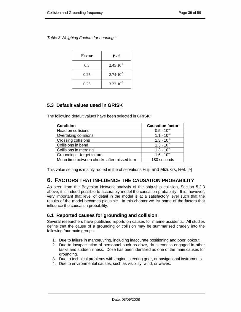
Table 3 Weighing Factors for headings:
5.3 Default values used in GRISK The following default values have been selected in GRISK:
Condition Causation factor Head on collisions 0.5 · 10-4 Overtaking collisions 1.1 · 10-4 Crossing collisions 1.3 · 10-4 Collisions in bend 1.3 · 10-4 Collisions in merging 1.3 · 10-4 Grounding – forget to turn 1.6 · 10-4 Mean time between checks after missed turn 180 seconds
This value setting is mainly rooted in the observations Fujii and Mizuki’s, Ref. [9]
6. FACTORS THAT INFLUENCE THE CAUSATION PROBABILITY As seen from the Bayesian Network analysis of the ship-ship collision, Section 5.2.3 above, it is indeed possible to accurately model the causation probability. It is, however, very important that level of detail in the model is at a satisfactory level such that the results of the model becomes plausible. In this chapter we list some of the factors that influence the causation probability.
6.1 Reported causes for grounding and collision Several researchers have published reports on causes for marine accidents. All studies define that the cause of a grounding or collision may be summarised crudely into the following four main groups:
1. Due to failure in manoeuvring, including inaccurate positioning and poor lookout. 2. Due to incapacitation of personnel such as doze, drunkenness engaged in other
tasks and sudden illness. Doze has been identified as one of the main causes for grounding.
3. Due to technical problems with engine, steering gear, or navigational instruments. 4. Due to environmental causes, such as visibility, wind, or waves.
Factor P ⋅ f
0.5 2.45·10-5
0.25 2.74·10-5
0.25 3.22·10-5

Collision and Grounding frequency Page 40 of 59
Date: 03/09/2008
Group 1 and 2 in the list above represent the contribution from human errors. Unquestionable, human error is an important cause to navigational accidents – perhaps dominant, as it is quoted that human errors account for at least2 80% of all accidents. More precisely it could be stated that approximately 80% of navigational accidents involves at least some human errors or questionable judgements rounded in organisational factors. What complicates the assessment is that the blame (or cause) for an accident can be allocated in different ways according to the perspective of the investigator. Typically a serious accidents start from basic human errors but the seriousness of the accident is rather a compound of a set of technical failure, operators’ error, fundamental design errors, and management errors. Therefore, any realistic modelling must provide a detailed representation of human error in order to be successful. Unfortunately, the human error mechanisms differ from technical or environmental cause (viz. the remaining 20%), and are – in fact – not yet well understood. A major problem in this respect is that there exists no such thing as a recipe for doing a specific task in the right way (e.g. performing a turn). In an examination of a series of manoeuvring simulation that have led to a grounding accident, Thau [29] found that the primary human error leading to the accident often occurred more than 10 minutes prior to the accident. Contrary, technical or environmental causes are generally simpler to model and understand.
6.1.1 Human and Organisational Errors Human errors can be described as actions taken by individuals that can lead an activity (design, construction, and operation) to realise a quality lower than intended. Human errors also include actions not taken, as these also may lead an activity to realise a quality lower than intended. Many people typically think of human error as “operator error” or “cockpit error”, in which the operator makes a slip or mistake due to misperceptions, faulty reasoning, inattention, or debilitating attributes such as sickness, drugs, or fatigue. However, there are many other important sources of human error. These includes factors such as management policies which pressure shipmasters to stay on schedule at all costs, poor equipment design which impedes the operator’s ability to perform a task, improper or lack of maintenance, improper or lack of training, and inadequate number of crew to perform a task. The human error factors range from those of judgement to ignorance, folly, and mischief. Inadequate training is the primary contributor to many of the past failures in marine structures. Also boredom has played a major role in many accidents. Based on a study by Bea [1] of human error factors in marine engineering the following primary factors were identified: Inadequate training Carelessness Ego
Physical limitations Wishful thinking Laziness
Inadequate communication Ignorance Greed
Bad judgement Negligence Alcohol Fatigue Folly Mischief Boredom Panic Violations
2 Some researchers even argue that 100% of all accidents are due to human error, since poor man-machine interface, failure of instrumentation (should have been checked more properly), under design, etc. all may be attributed as the result of some sort of human error. Any design is the consequence of human decisions.

Collision and Grounding frequency Page 41 of 59
Date: 03/09/2008
Organisation errors are a departure from acceptable or desirable practice on the part of a group of individuals that results in unacceptable or undesirable results. Primary organisational error factors includes, [1]: Ineffective regulatory requirements
Production orientation Inequitable promotion / recognition
Poor planning / training Cost-profit incentives Ineffective monitoring
Poor communications Time pressures Ego
Low quality culture Rejection of information Negative incentives
Low worker morale Complex structure Violations For example, the goals set by the organisation may lead rational individuals to conduct certain operations in manner that the corporate management would not approve if they were aware of their reliability implications. Similarly, corporate management, under pressures to reduce costs and maintain schedules, may not provide the necessary resources required allowing adequately safe operations. Other types of organisation and management procedure that affect the system reliability include, for example, parallel processing such as developing design criteria at the same time as the structure is being designed – a procedure that may not be appropriate in economic terms according to the costs and uncertainties.
6.1.2 Human error evaluation To date, four methodologies have been developed or adapted for maritime use. These are: 1. The operator function model (OFM) type of task analysis 2. Cognitive task analysis 3. Skill assessment 4. Error analysis The OFM task analysis, developed in1986 by Mitchell and Miller, see Rasmussen [26], provides a breakdown of a function (such as avoiding collisions with neighbouring vessels) into the tasks that must be performed. This also includes the information needed to perform each task, and the decisions that direct the sequence of tasks. This type of task description is independent of the automation; that is, the same tasks, information, and decisions are required, regardless of whether they are performed by a human or by a machine. For example, in collision avoidance, other vessels must be detected, their relative motions analysed to determine whether there is a threat of collision, and a decision made regarding how to change own ship’s course or speed in order to avoid a potential collision. These tasks must be performed regardless of who (human or machine) executes them.
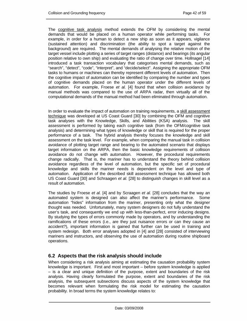
Collision and Grounding frequency Page 42 of 59
Date: 03/09/2008
The cognitive task analysis method extends the OFM by considering the mental demands that would be placed on a human operator while performing tasks. For example, in order for a human to detect a new ship as soon as it appears, vigilance (sustained attention) and discrimination (the ability to spot a target against the background) are required. The mental demands of analysing the relative motion of the target vessel include plotting a series of target ranges (distance) and bearings (its angular position relative to own ship) and evaluating the ratio of change over time. Hollnagel [14] introduced a task transaction vocabulary that categorises mental demands, such as “search”, “detect”, “code”, “interpret”, and “decide/select”. Assigning the appropriate OFM tasks to humans or machines can thereby represent different levels of automation. Then the cognitive impact of automation can be identified by comparing the number and types of cognitive demands placed on the human operator under the different levels of automation. For example, Froese et al. [4] found that when collision avoidance by manual methods was compared to the use of ARPA radar, then virtually all of the computational demands of the manual method had been eliminated through automation.
In order to evaluate the impact of automation on training requirements, a skill assessment technique was developed at US Coast Guard [30] by combining the OFM and cognitive task analyses with the Knowledge, Skills, and Abilities (KSA) analysis. The skill assessment is performed by taking each cognitive task (from the OFM/cognitive task analysis) and determining what types of knowledge or skill that is required for the proper performance of a task. The hybrid analysis thereby focuses the knowledge and skill assessment on the task level. For example, when comparing the manual task in collision avoidance of plotting target range and bearing to the automated scenario that displays target information on the ARPA, then the basic knowledge requirements of collision avoidance do not change with automation. However, the procedural requirements change radically. That is, the mariner has to understand the theory behind collision avoidance regardless of the level of automation, but the specific set of procedural knowledge and skills the mariner needs is dependent on the level and type of automation. Application of the described skill assessment technique has allowed both US Coast Guard [30] and Schraagen et al. [28] to distinguish changes in skill level as a result of automation. The studies by Froese et al. [4] and by Scraagen et al. [28] concludes that the way an automated system is designed can also affect the mariner’s performance. Some automation “hides” information from the mariner, presenting only what the designer thought was needed. Unfortunately, many system designers do not fully understand the user’s task, and consequently we end up with less-than-perfect, error inducing designs. By studying the types of errors commonly made by operators, and by understanding the ramifications of these errors (i.e., are they just nuisance errors or can they cause an accident?), important information is gained that further can be used in training and system redesign. Both error analyses adopted in [4] and [28] consisted of interviewing mariners and instructors, and observing the use of automation during routine shipboard operations.
6.2 Aspects that the risk analysis should include When considering a risk analysis aiming at estimating the causation probability system knowledge is important. First and most important – before system knowledge is applied – is a clear and unique definition of the purpose, extent and boundaries of the risk analysis. Having clearly formulated the purpose, extent and boundaries of the risk analysis, the subsequent subsections discuss aspects of the system knowledge that becomes relevant when formulating the risk model for estimating the causation probability. In broad terms the system knowledge relates to:
Collision and Grounding frequency Page 43 of 59
Date: 03/09/2008
• Configuration of the considered navigational area • Composition of the ship traffic in the area • Environmental conditions, such as weather, visibility, current, etc. • Configuration of considered vessel, such as main particulars, manoeuvrability, bridge
layout and procedures. Today, many ships have periodically unmanned engine rooms connected by computerised alarm systems to the bridge. Further, microcomputers for accounting, general record-keeping, and e-mail to land-based operations, automated satellite positioning systems (e.g., the global positioning system or GPS), navigation and collision-avoidance systems like electronic charts (ECDIS) and automated radar plotting aids (ARPA). With this boom in technology comes the concern that not all mariners understand how to use the automation effectively and safely. Indeed, there have been several “automation-assisted” accidents in recent years in which otherwise experienced mariners either did not know how to use the automated system or had trouble using it because of poor system design, Rothblum and Carvalhais [27]. The related human error modelling is best analysed using the cognitive task analysis. In a subsequent subsection the technical aspects of the different electronic systems is described.
6.2.1 Configuration of navigational area System knowledge of the configuration of the navigational area concerns the arrangement of the route in the vicinity of the considered area and identification of all difficulties in following the route before the considered location. Routes in the considered region that crosses the route prior to the considered location may have influence on the navigational safety and may thus indirectly have influence on faults at the considered location. The navigational markings, such as type of buoys that constitutes the routing system, must be identified. Further, presence and configuration of VTS system in the area as well as requirements for having pilot on board is part of the routing system. The purpose of the routing system is to improve the safety of navigation in converging areas and in areas where the density of traffic is great or where freedom of movement of shipping is inhibited by restricted sea-room, the existence of obstructions to navigation, limited depths and unfavourable meteorological conditions. This subsection describes some relevant aspects of the routing system. Navigational route, markings, aids, and restrictions Traffic lane - An area within defined limits in which one-way traffic is established. Natural obstacles, including those forming separation zones, may constitute a boundary. Traffic Separation Scheme - A routing measure aimed at the separation of opposing streams of traffic by appropriate means and by establishment of traffic lanes. Separation zone and lines - A zone or line separating the traffic lanes in which ships are proceeding in opposite or nearly opposite directions; or separating a traffic lane from the adjacent sea area; or separating traffic lanes designated for particular classes of ship proceeding in the same direction.
Collision and Grounding frequency Page 44 of 59
Date: 03/09/2008
Inshore traffic zone - A routing measure comprising a designated area between the landward boundary of a traffic separation scheme and the adjacent coast, to be used in accordance with the provision of amendment to International Regulations for Preventing Collision at Sea, 1972 (Collision Regulations). Deep-water route - A route within defined limits that have been accurately surveyed for clearance of sea bottom and submerged obstacles as indicated on the charts. Precautionary areas - A routing measure comprising an area within defined limits where ships must navigate with particular caution and within which the direction of traffic flow may be recommended. Navigational complications Complications that may impinge on the operational safety, e.g. bridges, multiple routes, crossing traffic, etc. Local and regional bathymetry Have an influence on the vessel sizes that are able to operate in the area – or collide with specific obstacles. The distance from the route to the ground affects Pc for both collision and grounding. VTS system A VTS system is typically present in areas of high navigational complexity where an accurate monitoring or guidance of the vessels in the area is of importance. Typical such areas may be near location of large bridges, areas with high rate of icebergs, or highly trafficked areas. The main effect of a VTS system, for a ship in contact with the VTS system, will be on the selection of route and distribution of ships across the routes. Reportedly, Olsen et al. [22] found that the effect of the presence of a VTS system might reduce the causation probability for ship-bridge collisions by a factor of 2 to 3. VTS systems may consist of the following equipment in different configurations, Olsen et al. [22]: • Radar installations • VHF radio and VHF direction finder • Closed Circuit Television • Infrared Television • Presence of a guard ship A VTS system consisting of only radar, VHF radio and VHF direction finder constitutes the basic system. Closed Circuit Television and Infrared Television are additional equipment. In some areas a guard ship may be attached to the VTS system. Ships participating in the VTS system must – if mandatory when entering the VTS area – report to the VTS centre via the VHF radio. Local authorities define the requirement to the ship sizes that should participate in the VTS system. According to the IMO regulation it is mandatory for vessels above 300 GRT to have VHF radio onboard.

Collision and Grounding frequency Page 45 of 59
Date: 03/09/2008
Some of the benefits of a VTS system is that the radar can detect navigational errors and thereby be corrected via the VHF communication. For ships violating the navigational regulations for the area, attempts can be made to establish contact with these over the VHF radio. Presence of Closed Circuit Television or Infrared Television allows for an improved surveillance of the navigation in the approach channels, for instance detecting a ship that omits to turn at a sea buoy or navigates of the channel. Presence of a guard ship may be able to help wandering vessels or like. This, of course, is highly dependent on the location of the guard ship and on the weather conditions. The degree of vessel participating in the VTS system varies considerably for different locations and is highly dependent on the presence of identifiable hazards in the waterway (e.g. fishing boats, icebergs, bridges, etc.). Presence of identifiable hazards increases the degree of participation. It should be noted that ship owners might obtain lower insurance premiums if their vessels participate in local VTS systems. This aspect therefore presents incitement to participate in the VTS system. The following probabilities of a vessel not participating in the VTS system have been extracted from [22].
Participation conditions Probability of not participating
Reported by
Mandatory 1⋅10-4 Japanese studies
Mandatory in domestic waters 1⋅10-3 Canadian Coast Guard
Voluntary in domestic waters 0.01 to 0.4 U.S. Coast Guard
Voluntary in the Dover Strait 0.2 U.K. Department of Transport Moreover, in the event of a vessel not reporting to the VTS system, then almost all (>99%, [22]) vessels respond to a direct call if the VTS system broadcast position, speed and course of the vessel. Some vessels, however, have proved impossible to contact by VHF or from a guard ship. When receiving an advice by VHF from the VTS centre, Olsen et al. [22] also reports that an average of 90% to 95% comply with the VTS advice. It is noted that the compliance is dependent on the nature of the advice and on the credibility of the system with the mariner. Local conditions near the vessel and unknown to the VTS may prevent the ship operator from following the advice. Requirements for pilot on board In some navigational areas it is required that vessels above a specific size must take a pilot on board. Aspect that must be addressed relates to how well does the pilot inform the master of the vessel of navigational plans? What are standard procedures? Are there requirements to the pilot of specific knowledge of the manoeuvrability of the vessel? Etc.
6.2.2 Composition of ship traffic The vessels that operate at general international routes range from traditional sailing ships, leisure crafts and fishing vessels (whose courses are unpredictable) to large tankers that are confined to deep-water routes only. The large diversity in the vessel traffic composition must be taken properly into account. This concerns bulk carriers and tankers in ballast having poor manoeuvrability; container ships with high cruising speed, hard pressed to arrive at their designated terminals just in time. Smaller petroleum, chemical and gas tankers feeding depots around the region, tow-boats and barges requiring plenty of sea-room to manoeuvre, and passenger ferries crossing the considered operational route.

Collision and Grounding frequency Page 46 of 59
Date: 03/09/2008
Among the shipmasters of these vessels there is a wide variance in the interpretation of safety and the choice of accepting a particular standard, which varies from criteria used, the circumstances and in most cases opinion. In gathering information on the ship traffic, focus will normally be on the commercial traffic, since these always will represent the primary threat to the navigational area. Leisure traffic and local fishing activity, however, can disturb the commercial traffic and thus be a source of errors. The extent and pattern of this type of traffic should be quantified. Type, size, and frequency of vessels operating in the area should be registered. When combined with information of the configuration of the navigational area this information provides guidance of the possibility for performing evasive manoeuvres. In essence, more ships mean more risks! For long-term design purposes forecasting of traffic intensity and composition is important. In this respect local bathymetry provides guidance for limiting vessel sizes, at least with respect to draft.
6.2.3 Environmental conditions The annual conditions for • Weather condition, • wind variations, cross wind and in sailing direction • waves, • visibility (fog, precipitation) • current variations, cross current and in sailing direction • ice conditions Major parts of these aspects were addressed in Friis Hansen and Pedersen [10].
6.2.4 Configuration of considered vessel Aspects that should be described • Vessel type and particulars: speed, profile. • Manoeuvrability of considered vessel • Layout of Man-Machine interface • Number of officers on the bridge • Instrumentation: ARPA, ECDIS, GPS, collision avoidance, and track keeping, etc. In the last few years, the Electronic Chart Display and Information System (ECDIS) has emerged as a powerful addition to the modern bridge. ECDIS offers the possibility for major changes in the navigation process and improves the safety and efficiency of maritime operations. By superimposing three items: a chart, the ship's real-time position, and radar on one display, ECDIS has the potential to improve the accuracy of navigation, increase awareness of dangerous conditions, and reduce the mariner's workload. At US Coast Guard, [30], the potential effects of these systems on bridge operations were examined, using the controlled conditions possible on a full-mission simulator. Four issues were examined: the potential of ECDIS to contribute to navigational precision, its potential to reduce navigation workload, the chart features and navigation functions required by the mariner, and the potential contribution of the integration of radar features on ECDIS. The results provided support to the U.S. position on the International Maritime Organization's (IMO) Standards for ECDIS and recommendations for future system design and for the incorporation of the system in bridge operations, [30].
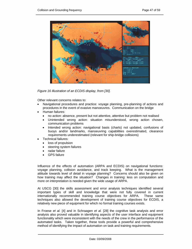
Collision and Grounding frequency Page 47 of 59
Date: 03/09/2008
Figure 16 Illustration of an ECDIS display, from [30].
Other relevant concerns relates to: • Navigational procedures and practice: voyage planning, pre-planning of actions and
procedures in the event of evasive manoeuvres. Communication on the bridge • Human failures:
• no action: absence, present but not attentive, attentive but problem not realised • Unintended wrong action: situation misunderstood, wrong action chosen,
communication problems • Intended wrong action: navigational basis (charts) not updated, confusions of
buoys and/or landmarks, manoeuvring capabilities overestimated, clearance requirements underestimated (relevant for ship-bridge collisions)
• Technical failures: • loss of propulsion • steering system failures • radar failure • GPS failure
Influence of the effects of automation (ARPA and ECDIS) on navigational functions: voyage planning, collision avoidance, and track keeping. What is the management attitude towards level of detail in voyage planning? Concerns should also be given on how training may affect the situation? Changes in training: less on computation and more on interpretation is needed given the wide usage of ARPA. At USCG [30] the skills assessment and error analysis techniques identified several important types of skill and knowledge that were not fully covered in current internationally recommended training course objectives for ARPA. These same techniques also allowed the development of training course objectives for ECDIS, a relatively new piece of equipment for which no formal training courses exists. In Froese et al. [4] and in Schraagen et al. [28] the cognitive task analysis and error analysis also proved valuable in identifying aspects of the user interface and equipment functionality which were inconsistent with the needs of the crew in the performance of the automated tasks. Taken together, these tools provide a powerful and comprehensive method of identifying the impact of automation on task and training requirements.

Collision and Grounding frequency Page 48 of 59
Date: 03/09/2008
7. SHIP TYPES USED IN THE GRISK PROGRAM The GRISK-program uses internally the following 14 ship types
GRISK Shiptype Ship Code
Crude oil tanker 1 This seems as a large and homogenous group
Oil products tanker 2 This is chosen because the oil products carried by this type, has different properties than crude oil.
Chemical tanker 3
Chemical tankers have generally more separate tanks than other tankers. They carry chemicals which in many cases are dissolved in the ocean when spilled. This is why marginal types such as wine and juice tanks are included here.
Gas tanker 4 Present a different risk (explosion) than oil and chemical tankers Container ship 5 Often fast ships. It could be categorized as just cargo General cargo ship 6 Often older and slower ships. It could be categorized as just cargoBulk carrier 7 This seems as a large and homogenous group
Ro-Ro cargo ship 8 This could also be classified as just cargo. It has been chosen because of its special stability problems
Passenger ship 9 All ships carrying more than 12 passengers sailing less than 30 knots
Fast ferry 10 All passenger ships sailing faster than 30 knots. Lloyds do not have a category for this
Support ship 11 A large group consisting mainly of small and slow work related crafts. However it also includes supply ships, tugs and pilots. They typical sail more randomly than larger ships
Fishing ship 12
Most fishing ships do not carry an AIS transponder but from a collision analysis point of view there present could be important. There is of course also the question of whether the ship is fishing or just sailing. This I believe is included in the activity part of the AIS data
Other ship 13 All other. Includes naval ships
Pleasure boat 14 Is not relevant for AIS, but from a collision analysis point of view they would be nice to include.
8. CONCLUSION A complete procedure has been presented for the analysis of grounding and ship-ship collision rates and the associated damage caused by collisions. The procedure has been applied to analysis of grounding and collision risks for selected geographical areas (Sea of Aaland and Bornholms Gat / Baltic West). These studies have not yet been reported, but reference will be added when these reports are completed. The document also presents a risk-based framework for calculating the causation probability for grounding and collision. The causation factor for ship-ship collision has been calculated using a Bayesian Network model. The result of the analysis was compared to reported causation probabilities and surprisingly good agreement was obtained. In order to be fully complete, however, the modelling needs to be extended. The concern that needs to be addressed was also described in the present document.
Collision and Grounding frequency Page 49 of 59
Date: 03/09/2008
9. REFERENCES [1] Bea, R.: “The Role of Human Error in Design, Construction, and Reliability of
Marine Structures”. Technical report, Ship Structure Committee, 1994. SSC-378. [2] Comstock, J.P. and Robertson, J.B.: "Survival of Collision Damage Versus the
1960 Convention of Safety of Life at Sea", SNAME, pp. 461-522. 1961. [3] Cowi: "Risk analysis of oil and chemical spills in Danish waters", Minister of
Defence, 147 pages. 2007. (In Danish) [4] Froese, J, Hartung, R. and Schack, C.: “Risk Assessment for Solo Watchkeeping at
Night under Defined Conditions”. ISSUS, Germany. March, 1996. [5] Fujii, Y. Yamanouchi, H and Mizuki, N.: “Some Factors Affecting the Frequency of
Accidents in Marine Traffic. II: The probability of Stranding, III: The Effect of Darkness on the Probability of Stranding”. Journal of Navigation, Vol. 27, 1974.
[6] Fujii, Y. and Yamanouchi, H.: “Visual range and the Degree of Risk”, Journal Of Navigation Vol. 27, No. 2, pp 248- 252, 1974.
[7] Fujii, Y.: "Integrated Study on Marine Traffic Accidents", IABSE Colloquium on Ship Collision with Bridges and Offshore Structures, Copenhagen, Vol. 42, pp. 91-98. 1983.
[8] Fujii, Y., Yamanouchi, H. & Matui, T.: "Survey on Vessel Traffic Management Systems and Brief Introduction to Marine Traffic Studies", Electronic Navigation Research Institute Papers No. 45. 1984.
[9] Fujii, Y. and Mizuki, N.: “Design of VTS systems for water with bridges”. Proc. of the International Symposium on Advances in Ship Collision Analysis. Gluver & Olsen eds. Copenhagen, Denmark, 10-13 May, 1998. pp. 177-190.
[10] Friis Hansen, P and Pedersen, P.T.: "Risk Analysis of Conventional and Solo Watch Keeping” Submitted to Int. Maritime Organisation (IMO) Maritime Safety Committee by Denmark at the 69th Session. 1998.
[11] Friis-Hansen, P and Cerup Simonsen, B.: "Dogden Feasibility Studie 2001, Aktivitet 3.9, Søuheld”, December 2001, HLD Joint Venture”
[12] Gluver, H. and Olsen, D.: “Current practice in risk analysis of ship collisions to bridges”. Proc. of the International Symposium on Advances in Ship Collision Analysis. Gluver & Olsen eds. Copenhagen, Denmark, 10-13 May, 1998. pp. 85-96.
[13] Haugen, S.: “Probabilistic Evaluation of Frequency of Collision Between Ships and Offshore Platforms”. Ph.D. thesis, Marine Structures, University of Trondheim. Aug. 1991.
[14] Hollnagel, E.: “A Cognitive Task Analysis of the STGR Scenario”. Nordic nuclear safety research (NKS). NKS/RAK-1(96)R3. April 1996.
[15] IMO: "Resolution and Other Decisions", Resolution 680-732, London. 1992. [16] Inoue, K.: "On the Separation of Traffic at Straight Waterway by Distribution Model
of Ship Paters", J. Nautical Society of Japan, No. 5. 1972. [17] ISESO: "Information Technology for Enhanced Safety and Efficiency in Ship Design
and Operation", Danish Maritime Authority. http://www.sofartsstyrelsen.dk/sw1161.asp
[18] Jensen, F.V.: “An Introduction to Bayesian Networks”. UCL Press. 1996. [19] Karlson, M. Rasmussen, F. and Frisk, L: “Verification of ship collision frequency
model”. Proc. of the International Symposium on Advances in Ship Collision Analysis. Gluver & Olsen eds. Copenhagen, Denmark, 10-13 May, 1998. pp. 117-121.
[20] Larsen, O. Damgaard: “Ship Collisions with Bridges – The interaction between Vessel Traffic and Bridge Structures”. Structural Engineering Documents 4. International Association for Bridge and Structural Engineering. 1993.

Collision and Grounding frequency Page 50 of 59
Date: 03/09/2008
[21] MacDuff, T.: “The Probability of Vessel Collisions”. Ocean Industry, September 1974. pp. 144-148.
[22] Olsen, D. Gotfredsen, H.H. and Fujii, Y.: “Risk Reducing Effects of the Great Belt VTS System”. 7th International VTS Symposium, Vancouver, Canada, June 1992.
[23] Pearl, J.: “Probabilistic Reasoning in Intelligent Systems: Networks of Plausible Inference”. Morgan Kaufmann Publishers, Inc. 1988.
[24] Pedersen, P. Terndrup, Hansen, P. Friis, and Nielsen, L.: “Probabilistic Analysis of Collision Damages With Application to Passenger Ro-Ro Vessels”. Safety of Passenger Ro-Ro Vessels. Dept. of Naval Architecture and Ocean Eng. Doc. pac-001. 1995.
[25] Pedersen, P. Terndrup: "Collision and Grounding Mechanics". Proc. WEMT 1995, Copenhagen, Volume 1, pp.125-157. 1995.
[26] Rasmussen, B. and Whetton, C.: “Hazard Identification Based on Plant Functional Modelling”. Risø National Laboratory, Roskilde, Denmark. October 1993.
[27] Rothblum, A. M. and Carvalhais, A.B.: “Maritime Applications of Human Factors Test and Evaluation”. Chapter 15 in the book, Handbook of Human Factors Testing and Evaluation, edited by T. G. O'Brien and S. G. Charlton, Mahwah, NJ: Lawrence Erlbaum Assoc., 1996.
[28] Schraagen, J.M.C, van Breda, L., and Rasker, P.C.: “Sole look-out during periods of darkness”. TNO Human Factors Rresearch Institute. August 22, 1997.
[29] Thau, J. Personal communication. Danish Maritime Institute, Denmark. 1999. [30] U.S. Coast Guard: Homepage of Research and Development Center.
http://www.rdc.uscg.mil

Collision and Grounding frequency Page 51 of 59
Date: 03/09/2008
Appendix: Used ship types compared to the types defined in the Lloyds data base The GRISK-program uses internally the following 14 ship types
GRISK Shiptype Ship Code
Crude oil tanker 1 This seems as a large and homogenous group
Oil products tanker 2 This is chosen because the oil products carried by this type, has different properties than crude oil.
Chemical tanker 3
Chemical tankers have generally more separate tanks than other tankers. They carry chemicals which in many cases are dissolved in the ocean when spilled. This is why marginal types such as wine and juice tanks are included here.
Gas tanker 4 Present a different risk (explosion) than oil and chemical tankers Container ship 5 Often fast ships. It could be categorized as just cargo General cargo ship 6 Often older and slower ships. It could be categorized as just cargoBulk carrier 7 This seems as a large and homogenous group
Ro-Ro cargo ship 8 This could also be classified as just cargo. It has been chosen because of its special stability problems
Passenger ship 9 All ships carrying more than 12 passengers sailing less than 30 knots
Fast ferry 10 All passenger ships sailing faster than 30 knots. Lloyds do not have a category for this
Support ship 11 A large group consisting mainly of small and slow work related crafts. However it also includes supply ships, tugs and pilots. They typical sail more randomly than larger ships
Fishing ship 12
Most fishing ships do not carry an AIS transponder but from a collision analysis point of view there present could be important. There is of course also the question of whether the ship is fishing or just sailing. This I believe is included in the activity part of the AIS data
Other ship 13 All other. Includes naval ships
Pleasure boat 14 Is not relevant for AIS, but from a collision analysis point of view they would be nice to include.
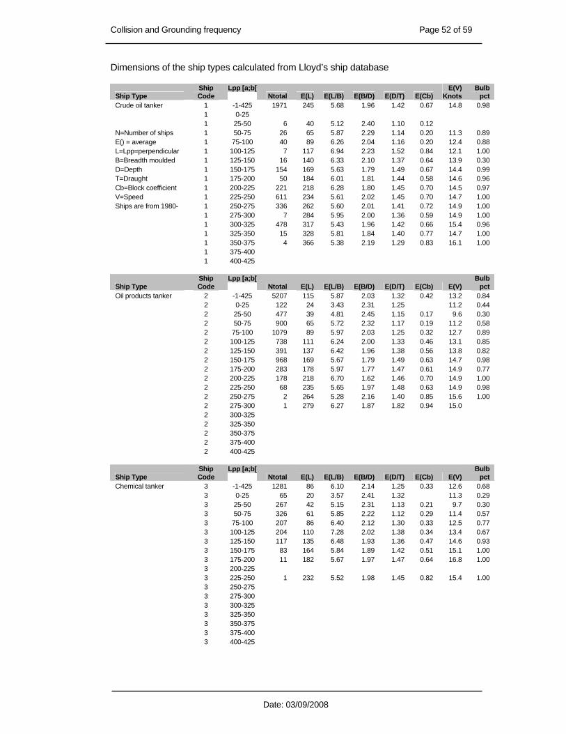
Collision and Grounding frequency Page 52 of 59
Date: 03/09/2008
Dimensions of the ship types calculated from Lloyd’s ship database
Ship Type Ship Code
Lpp [a;b[ Ntotal E(L) E(L/B) E(B/D) E(D/T) E(Cb)
E(V) Knots
Bulb pct
Crude oil tanker 1 -1-425 1971 245 5.68 1.96 1.42 0.67 14.8 0.98 1 0-25 1 25-50 6 40 5.12 2.40 1.10 0.12 N=Number of ships 1 50-75 26 65 5.87 2.29 1.14 0.20 11.3 0.89 E() = average 1 75-100 40 89 6.26 2.04 1.16 0.20 12.4 0.88 L=Lpp=perpendicular 1 100-125 7 117 6.94 2.23 1.52 0.84 12.1 1.00 B=Breadth moulded 1 125-150 16 140 6.33 2.10 1.37 0.64 13.9 0.30 D=Depth 1 150-175 154 169 5.63 1.79 1.49 0.67 14.4 0.99 T=Draught 1 175-200 50 184 6.01 1.81 1.44 0.58 14.6 0.96 Cb=Block coefficient 1 200-225 221 218 6.28 1.80 1.45 0.70 14.5 0.97 V=Speed 1 225-250 611 234 5.61 2.02 1.45 0.70 14.7 1.00 Ships are from 1980- 1 250-275 336 262 5.60 2.01 1.41 0.72 14.9 1.00 1 275-300 7 284 5.95 2.00 1.36 0.59 14.9 1.00 1 300-325 478 317 5.43 1.96 1.42 0.66 15.4 0.96 1 325-350 15 328 5.81 1.84 1.40 0.77 14.7 1.00 1 350-375 4 366 5.38 2.19 1.29 0.83 16.1 1.00 1 375-400 1 400-425
Ship Type Ship Code
Lpp [a;b[ Ntotal E(L) E(L/B) E(B/D) E(D/T) E(Cb) E(V)
Bulb pct
Oil products tanker 2 -1-425 5207 115 5.87 2.03 1.32 0.42 13.2 0.84 2 0-25 122 24 3.43 2.31 1.25 11.2 0.44 2 25-50 477 39 4.81 2.45 1.15 0.17 9.6 0.30 2 50-75 900 65 5.72 2.32 1.17 0.19 11.2 0.58 2 75-100 1079 89 5.97 2.03 1.25 0.32 12.7 0.89 2 100-125 738 111 6.24 2.00 1.33 0.46 13.1 0.85 2 125-150 391 137 6.42 1.96 1.38 0.56 13.8 0.82 2 150-175 968 169 5.67 1.79 1.49 0.63 14.7 0.98 2 175-200 283 178 5.97 1.77 1.47 0.61 14.9 0.77 2 200-225 178 218 6.70 1.62 1.46 0.70 14.9 1.00 2 225-250 68 235 5.65 1.97 1.48 0.63 14.9 0.98 2 250-275 2 264 5.28 2.16 1.40 0.85 15.6 1.00 2 275-300 1 279 6.27 1.87 1.82 0.94 15.0 2 300-325 2 325-350 2 350-375 2 375-400 2 400-425
Ship Type Ship Code
Lpp [a;b[ Ntotal E(L) E(L/B) E(B/D) E(D/T) E(Cb) E(V)
Bulb pct
Chemical tanker 3 -1-425 1281 86 6.10 2.14 1.25 0.33 12.6 0.68 3 0-25 65 20 3.57 2.41 1.32 11.3 0.29 3 25-50 267 42 5.15 2.31 1.13 0.21 9.7 0.30 3 50-75 326 61 5.85 2.22 1.12 0.29 11.4 0.57 3 75-100 207 86 6.40 2.12 1.30 0.33 12.5 0.77 3 100-125 204 110 7.28 2.02 1.38 0.34 13.4 0.67 3 125-150 117 135 6.48 1.93 1.36 0.47 14.6 0.93 3 150-175 83 164 5.84 1.89 1.42 0.51 15.1 1.00 3 175-200 11 182 5.67 1.97 1.47 0.64 16.8 1.00 3 200-225 3 225-250 1 232 5.52 1.98 1.45 0.82 15.4 1.00 3 250-275 3 275-300 3 300-325 3 325-350 3 350-375 3 375-400 3 400-425

Collision and Grounding frequency Page 53 of 59
Date: 03/09/2008
Ship Type Ship Code Lpp [a;b[ Ntotal E(L) E(L/B) E(B/D) E(D/T) E(Cb) E(V)
Bulb pct
Gas tanker 4 -1-425 1037 139 5.82 1.95 1.56 0.41 15.1 0.92 4 0-25 3 2.13 1.74 12.2 1.00 4 25-50 21 44 4.63 2.83 1.31 0.18 10.2 0.80 4 50-75 211 63 5.36 2.21 1.23 0.23 12.2 0.82 4 75-100 261 90 5.74 2.12 1.37 0.40 13.3 0.94 4 100-125 131 110 6.14 1.83 1.40 0.44 14.9 0.90 4 125-150 55 142 6.14 1.66 1.55 0.56 16.0 0.82 4 150-175 56 163 6.02 1.57 1.66 0.58 16.2 1.00 4 175-200 11 191 6.17 1.60 1.73 0.66 16.4 1.00 4 200-225 107 215 6.01 1.73 1.81 0.57 16.6 0.93 4 225-250 3 230 5.99 1.51 2.22 0.47 17.7 1.00 4 250-275 129 268 6.07 1.72 2.17 0.44 19.7 1.00 4 275-300 49 278 6.04 1.78 2.22 0.32 19.6 1.00 4 300-325 4 325-350 4 350-375 4 375-400 4 400-425
Ship Type Ship Code Lpp [a;b[ Ntotal E(L) E(L/B) E(B/D) E(D/T) E(Cb) E(V)
Bulb pct
Container ship 5 -1-425 4678 176 6.48 1.84 1.48 0.27 19.8 0.99 5 0-25 101 23 3.47 1.76 1.54 0.26 22.2 1.00 5 25-50 25 40 4.83 2.06 1.35 0.11 11.5 5 50-75 94 65 5.43 2.25 1.36 0.10 12.5 0.85 5 75-100 370 89 5.67 2.08 1.37 0.24 14.2 0.96 5 100-125 615 114 6.01 1.93 1.37 0.26 16.3 0.99 5 125-150 886 137 6.17 1.89 1.41 0.26 18.6 0.99 5 150-175 669 162 6.09 1.89 1.44 0.31 19.0 1.00 5 175-200 517 190 6.34 1.80 1.50 0.21 20.8 1.00 5 200-225 249 212 6.76 1.75 1.52 0.27 21.4 1.00 5 225-250 264 237 7.37 1.68 1.59 0.32 22.6 1.00 5 250-275 409 263 7.33 1.62 1.69 0.28 24.3 1.00 5 275-300 327 283 8.09 1.58 1.66 0.32 24.4 1.00 5 300-325 105 315 7.29 1.76 1.72 0.18 25.0 1.00 5 325-350 36 333 7.78 1.71 1.71 0.50 25.0 1.00 5 350-375 10 361 7.58 1.81 1.72 0.66 25.0 1.00 5 375-400 1 376 6.67 1.87 1.89 0.63 25.0 1.00 5 400-425
Ship Type Ship Code Lpp [a;b[ Ntotal E(L) E(L/B) E(B/D) E(D/T) E(Cb) E(V)
Bulb pct
General cargo ship 6 -1-425 9457 87 5.89 2.03 1.40 0.22 12.5 0.80 6 0-25 413 21 3.11 2.29 1.38 0.13 11.3 0.56 6 25-50 1101 41 4.88 2.19 1.38 0.12 10.0 0.64 6 50-75 2690 63 5.62 2.02 1.46 0.10 11.0 0.82 6 75-100 2894 87 5.95 2.00 1.35 0.25 12.3 0.79 6 100-125 1180 110 6.55 2.07 1.39 0.34 13.3 0.69 6 125-150 668 138 6.73 1.94 1.40 0.36 14.8 0.83 6 150-175 300 161 6.35 1.80 1.41 0.33 15.6 0.99 6 175-200 208 183 6.20 1.79 1.42 0.31 15.7 0.98 6 200-225 2 202 6.53 1.75 1.51 0.76 15.8 1.00 6 225-250 1 237 7.35 1.76 1.55 0.67 20.5 6 250-275 6 275-300 6 300-325 6 325-350 6 350-375 6 375-400 6 400-425

Collision and Grounding frequency Page 54 of 59
Date: 03/09/2008
Ship Type Ship Code
Lpp [a;b[ Ntotal E(L) E(L/B) E(B/D) E(D/T) E(Cb) E(V)
Bulb pct
Bulk carrier 7 -1-425 6090 185 6.14 1.87 1.41 0.30 14.1 0.96 7 0-25 63 2.18 1.35 13.5 0.80 7 25-50 160 44 4.07 2.46 1.41 0.19 10.1 0.64 7 50-75 263 62 4.92 2.13 1.42 0.18 10.9 0.78 7 75-100 121 88 5.54 2.19 1.35 0.27 12.1 0.75 7 100-125 212 111 6.22 1.98 1.37 0.32 13.1 0.77 7 125-150 396 141 5.91 1.91 1.39 0.20 13.9 0.96 7 150-175 1032 165 6.22 1.88 1.41 0.27 14.3 0.98 7 175-200 1556 182 6.03 1.83 1.45 0.27 14.4 0.99 7 200-225 1376 216 6.70 1.72 1.40 0.33 14.5 0.98 7 225-250 174 235 6.57 1.90 1.43 0.45 14.3 0.89 7 250-275 255 262 6.02 1.85 1.38 0.53 14.2 0.98 7 275-300 431 281 6.12 1.89 1.36 0.32 14.6 0.99 7 300-325 47 307 6.16 2.02 1.40 0.39 13.9 1.00 7 325-350 4 327 5.64 1.87 1.39 0.63 13.8 1.00 7 350-375 7 375-400 7 400-425
Ship Type Ship Code
Lpp [a;b[ Ntotal E(L) E(L/B) E(B/D) E(D/T) E(Cb) E(V)
Bulb pct
Ro-Ro cargo ship 8 -1-425 1161 123 5.24 2.42 1.91 0.16 16.7 0.87 8 0-25 47 22 3.23 3.38 1.63 0.18 10.4 0.09 8 25-50 292 40 4.11 3.57 1.35 0.05 9.5 8 50-75 137 58 4.52 3.63 1.44 0.10 9.9 0.23 8 75-100 61 90 5.13 2.28 1.67 0.23 14.5 0.93 8 100-125 58 111 5.71 2.23 1.66 0.23 16.5 1.00 8 125-150 60 141 6.00 2.05 1.90 0.18 18.1 0.96 8 150-175 228 166 5.55 1.82 2.21 0.21 18.8 0.99 8 175-200 257 188 5.93 1.58 2.43 0.20 19.3 1.00 8 200-225 12 216 6.70 1.38 2.60 0.25 20.2 1.00 8 225-250 9 236 7.31 1.79 1.56 0.48 20.0 0.88 8 250-275 8 275-300 8 300-325 8 325-350 8 350-375 8 375-400 8 400-425
Ship Type Ship Code
Lpp [a;b[ Ntotal E(L) E(L/B) E(B/D) E(D/T) E(Cb) E(V)
Bulb pct
Passenger ship 9 -1-425 2999 80 4.78 2.72 1.81 0.16 17.9 0.61 9 0-25 489 22 2.96 2.90 1.83 0.09 18.5 0.11 9 25-50 1134 35 3.93 2.95 1.76 0.09 16.8 0.19 9 50-75 406 61 4.59 3.00 1.64 0.15 14.1 0.53 9 75-100 225 86 5.21 2.60 1.83 0.19 15.5 0.56 9 100-125 147 112 5.76 2.27 1.82 0.27 18.0 0.81 9 125-150 190 136 5.89 2.12 2.02 0.27 19.8 0.95 9 150-175 175 162 6.26 2.37 1.89 0.25 21.6 0.95 9 175-200 122 184 6.73 2.09 2.05 0.22 23.4 0.99 9 200-225 38 215 6.89 2.09 2.28 0.23 20.8 1.00 9 225-250 33 238 6.96 2.54 1.82 0.31 21.6 1.00 9 250-275 36 263 8.01 2.33 2.10 0.26 22.9 1.00 9 275-300 1 275 7.13 3.30 1.33 22.1 1.00 9 300-325 3 303 7.69 2.64 1.90 24.5 1.00 9 325-350 9 350-375 9 375-400 9 400-425

Collision and Grounding frequency Page 55 of 59
Date: 03/09/2008
Ship Type Ship Code
Lpp [a;b[ Ntotal E(L) E(L/B) E(B/D) E(D/T) E(Cb) E(V)
Bulb pct
Fast ferry 10 -1-425 530 47 3.67 3.00 2.38 0.08 36.2 0.16 10 0-25 92 24 2.82 3.00 1.99 0.03 36.5 0.02 10 25-50 319 35 3.57 2.88 2.44 0.08 35.5 0.16 10 50-75 54 65 3.35 3.71 2.26 0.05 37.3 0.24 10 75-100 48 86 4.45 3.14 2.57 0.08 38.2 0.22 10 100-125 8 112 4.94 2.76 2.77 0.12 38.9 0.43 10 125-150 6 128 5.57 2.22 2.73 0.08 40.5 10 150-175 10 175-200 1 191 7.24 1.68 2.15 0.58 32.0 1.00 10 200-225 2 208 8.00 1.40 2.51 30.5 1.00 10 225-250 10 250-275 10 275-300 10 300-325 10 325-350 10 350-375 10 375-400 10 400-425
Ship Type Ship Code
Lpp [a;b[ Ntotal E(L) E(L/B) E(B/D) E(D/T) E(Cb) E(V)
Bulb pct
Support ship 11 -1-425 12006 42 3.63 2.32 1.33 0.19 13.0 0.13 11 0-25 3292 22 2.94 2.27 1.35 0.37 12.4 0.02 11 25-50 5671 32 3.39 2.28 1.33 0.12 13.1 0.05 11 50-75 2293 60 4.34 2.45 1.28 0.15 13.0 0.28 11 75-100 450 83 4.68 2.41 1.34 0.22 13.9 0.46 11 100-125 129 112 5.25 2.30 1.53 0.22 13.7 0.60 11 125-150 52 134 5.25 2.29 1.57 0.32 14.7 0.52 11 150-175 23 160 5.44 2.46 1.49 0.20 14.8 0.47 11 175-200 8 189 5.79 1.86 1.61 0.42 12.3 0.80 11 200-225 25 213 5.74 1.93 1.48 0.40 12.7 0.82 11 225-250 34 235 5.59 1.89 1.46 0.49 13.3 0.75 11 250-275 11 263 5.64 1.86 1.45 0.37 13.4 1.00 11 275-300 8 284 5.23 1.97 1.39 0.34 14.5 0.33 11 300-325 7 308 5.46 1.95 1.38 0.41 14.5 1.00 11 325-350 3 329 5.29 2.05 1.33 0.82 15.1 1.00 11 350-375 11 375-400 11 400-425
Ship Type Ship Code
Lpp [a;b[ Ntotal E(L) E(L/B) E(B/D) E(D/T) E(Cb) E(V)
Bulb pct
Fishing ship 12 -1-425 8384 40 4.27 1.95 1.31 0.20 11.8 0.71 12 0-25 3009 22 3.16 2.00 1.27 0.16 10.2 0.39 12 25-50 3928 37 4.37 2.00 1.27 0.19 11.7 0.84 12 50-75 1109 56 4.93 1.80 1.38 0.25 13.6 0.74 12 75-100 267 89 5.76 1.66 1.65 0.40 14.8 0.55 12 100-125 64 108 5.90 1.65 1.68 0.42 15.2 0.69 12 125-150 3 132 6.37 1.93 1.49 0.25 15.8 12 150-175 4 165 6.11 2.23 1.58 0.72 14.6 0.25 12 175-200 12 200-225 12 225-250 12 250-275 12 275-300 12 300-325 12 325-350 12 350-375 12 375-400 12 400-425

Collision and Grounding frequency Page 56 of 59
Date: 03/09/2008
Ship Type Ship Code
Lpp [a;b[ Ntotal E(L) E(L/B) E(B/D) E(D/T) E(Cb) E(V)
Bulb pct
Other ship 13 -1-425 2047 69 4.05 3.06 1.61 0.16 15.4 0.44 13 0-25 585 21 3.09 3.40 1.81 0.15 22.0 0.11 13 25-50 502 36 3.59 3.12 1.52 0.21 14.2 0.39 13 50-75 383 61 4.19 2.91 1.48 0.13 13.3 0.58 13 75-100 281 86 4.10 3.05 1.60 0.13 15.0 0.54 13 100-125 145 111 4.35 3.14 1.81 0.13 16.2 0.44 13 125-150 53 136 5.52 2.57 1.39 0.08 13.8 0.50 13 150-175 34 164 5.22 2.47 1.99 0.32 15.4 1.00 13 175-200 37 188 6.23 1.94 1.62 0.25 18.4 1.00 13 200-225 15 215 5.75 2.64 1.62 0.46 14.3 0.67 13 225-250 4 239 4.60 2.79 2.67 0.31 13 250-275 2 257 4.28 2.00 1.43 13 275-300 1 294 4.74 1.93 1.46 13 300-325 13 325-350 13 350-375 13 375-400 13 400-425
Ship Type Ship Code
Lpp [a;b[ Ntotal E(L) E(L/B) E(B/D) E(D/T) E(Cb) E(V)
Bulb pct
Pleasure boat 14 -1-425 786 39 4.34 1.94 1.84 0.14 16.6 0.34 14 0-25 143 19 3.25 1.87 1.98 0.03 18.4 14 25-50 536 36 4.33 1.95 1.83 0.14 16.2 0.26 14 50-75 88 58 4.97 1.90 1.74 0.25 17.0 0.62 14 75-100 14 85 5.67 2.22 1.60 0.10 18.9 0.80 14 100-125 2 107 6.24 2.45 1.66 0.34 19.8 1.00 14 125-150 3 132 6.77 2.03 2.03 0.19 25.0 14 150-175 14 175-200 14 200-225 14 225-250 14 250-275 14 275-300 14 300-325 14 325-350 14 350-375 14 375-400 14 400-425
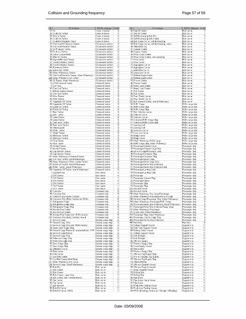
Collision and Grounding frequency Page 57 of 59
Date: 03/09/2008

Collision and Grounding frequency Page 58 of 59
Date: 03/09/2008
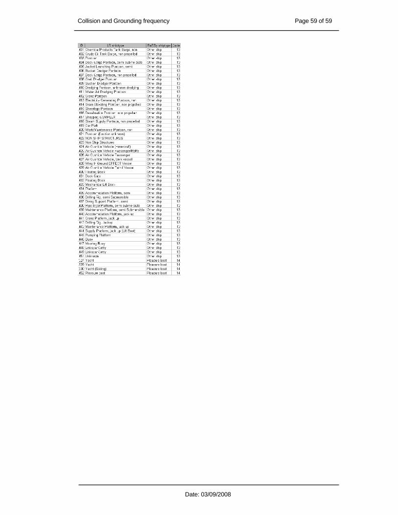
Collision and Grounding frequency Page 59 of 59
Date: 03/09/2008