ITSM2000 - Home | York University · AR-Model>Estimation>Burg or AR-Model>Estimation>Yule-Walker....

ITSM2000GETTING STARTEDACF/PACFARAR ForecastsARMA ForecastsAutofitBox-Cox TransformationClassical DecompositionColor CustomizationConstrained MLECross-correlationsCross-spectrumData setsData transferDifferencingExponential smoothingFisher's TestGARCH modelsGraphsHolt-Winters ForecastsHolt-Winters Seasonal ForecastsIntervention AnalysisLong Memory ModelsMaximum Likelihood EstimationModel RepresentationsModel SpecificationModel Spectral DensityMoving Average SmoothingMultivariate AutoregressionPeriodogramPreliminary EstimationProject EditorRegression with ARMA or ARFIMA ErrorsResidual PlotsResidual TestsSimulationSpectral Smoothing (FFT)SubsequenceSubtract MeanTransfer Function ModellingTSM Files

GETTING STARTED: CREATING, EDITING AND SAVING PROJECTS

See also Graphs, TSM Files.

Creating your own project. If you have observations X(1),…,X(n), of a univariate or m-variate time series which you wish to analyze with ITSM, the data should be stored as an ASCII file consisting of m columns (separated by a blank space), one for each component of the series. The file should be stored in the directory containing the program ITSM and given the suffix .TSM so that it will be recognized by the program. It will then appear together with the data files included in the package when you open a project as described in the following paragraph.

Opening a project. Run the program ITSM by either double-clicking on the ITSM icon in the ITSM2000 folder or by typing ITSM in a DOS window open in the ITSM2000 directory. From the top-left corner of the ITSM window select the options File>Project>Open, then choose Univariate or Multivariate and click OK. A window showing all of the .TSM files in the ITSM2000 directory will then appear and you can select the desired project either by double-clicking on its icon or by typing the project name (e.g.AIRPASS) and clicking on OK to open the project (AIRPASS.TSM). If you chose to open a multivariate project you will then be asked to specify the number m of components in each observation vector.Having done this and clicked OK, you will see a graph of the data (or a graph of each component series if the data are multivariate). If the data appears to be from a non-stationary series you will need to make transformations before attempting to fit a stationary time series model. See Box-Cox Transformations, Differencing, Classical Decomposition.

Specifying a model. If the .TSM file contains only data (which is very often the case) then ITSM will assign the default model WN(0,1), i.e. white noise with variance 1, to the project. Of course this will usually be inappropriate so that you will wish to introduce a more appropriate model for the data after first transforming the series to stationarity as indicated above. Model specification can be done either directly or by a variety of estimation algorithms provided in the package. See Model Specification, Preliminary Estimation, Maximum Likelihood Estimation, Multivariate Autoregression.

PROJECTS. ITSM v.7.0(Professional) has the capacity to handle up to 10 projects simultaneously. Each project consists of a data file and a model. Projects can be manipulated with the aid of the Project Editor (see below).

Saving Data. At any time data such as the current series (the one displayed in the project window, which in general will be a transformed version of the original series), the sample ACF, and the residuals(if a model has been fitted) can be saved to an ASCII file or to the Clipboard, by selecting the options File>Export, completing the following dialogue box as appropriate and then clicking OK.

Saving Projects. The current data and fitted model can be saved together in a .TSM file by pressing the Save Project button, fourth from the left at the top of the ITSM screen. If the saved file is later opened in ITSM using the options File>Project>Open, then both the data and the accompanying model will be imported into the project.

Importing Files. If a project is already open, the data can be replaced by a new data set using the options File>Import File and selecting the file to be imported. If the imported file is a pure data file, then the model in the current project will be retained. If however the imported file contains a model then importing the file will cause the model in ITSM to be replaced by the model stored in the imported file.

Saving Graphs. Any graph which appears on the screen is most conveniently saved by right-clicking on it, selecting Copy to Clipboard and pasting it into an open Word or Wordpad document.

Saving Information. Highlighting a window and pressing the red INFO button (or right-clicking on the window and selecting Info) will open a new window containing printed information pertaining to the highlighted window. This can be saved by right clicking on the Information window, clicking on Select All, right-clicking again, clicking on Copy, and then pasting into an open Word or Wordpad document.

Managing Multiple Projects. It is often convenient, especially when dealing with multivariate time series, to have several projects in ITSM concurrently. The management of multiple projects is achieved with the project editor as described below.

THE PROJECT EDITOR. The project editor is opened by pressing the Project Editor button at the top left of the ITSM screen.

Example: Use the options File>Project>Open>Multivariate to open the project LS2.TSM, specifying 2 for the number of columns in the data. Then use File>Project>Open>Univariate to open the project LEAD.TSM, which happens to be the first component of LS2.TSM. Then press the Project Editor button, click on the plus signs beside each project and you will see the following window.

Renaming a series. The names of the series in each project can be changed by clicking on the current name to highlight it, then clicking again and typing the new name in the box surrounding the old title. When you are satisfied with the names press OK and the window will close. Changing the above names to reflect the contents of the series gives

When you are satisfied with the names press OK and the window will close. Either of the two projects can now be analyzed in ITSM. If the window labelled C:\ITSM2000\LEAD.TSM is

highlighted, you will see the univariate toolbar at the top of the ITSM screen and all the ITSM univariate functions (transformations, model-fitting etc.) can then be applied to the univariate data set LEAD.TSM. On the other hand, if the window labelled C:\ITSM2000\LS2.TSM is highlighted, then the multivariate toolbar will appear at the top or the ITSM screen and the ITSM multivariate functions (transformations, AR-Model, etc.) can then be applied to the multivariate data set LS2.TSM.Transferring series into a multivariate project: A series in any univariate or multivariate project can be transferred to a multivariate project with the aid of the project editor. Open the project editor, click on the plus signs beside each project, click on the series to be transferred and drag it to the top line of the project to which it is to be added. You will then be asked to confirm the data transfer. Applying this to our current example, we can move the univariate series LEAD into the project LS2 to get a trivariate project (with two identical copies of the LEAD series). The project editor window then appears as follows.

Click OK and you will see that the project LEAD.TSM now contains no data. This project (or any other project) can be closed by clicking on the X in the top right corner of the project window.

Tansferring a Component of a Multivariate Series to a Univariate Project. From an m-variate project, a univariate project with any component series as data can be created as follows. Select File>Project>New, check the option Univariate and click on OK. Open the project editor and click on the plus sign to the left of the multivariate project. Click on the component to be transferred and drag it to the line labeled New Univariate Project.You will then be asked to confirm the data transfer.. Once you have done this, a graph of the component series will appear in the New Univariate Project window and the univariate tool bar will appear at the top of the ITSM window.

Activating and Deactivating Series. In an m-variate project the maximum value of m for which cross-correlations can be plotted or to which a multivariate autoregression can be fitted is 5. If a multivariate series with more than 5 components is imported to ITSM, then it is necessary

to ensure that only five components are activated. Selection of the five to be activated is carried out with the Project Editor.

Example. Use File>Project>Open>Multivariate to open the project STOCK7.TSM. (This file contains the daily returns, 100ln[P(t)/P(t-1)] for seven stock indices, Australian, Dow-Jones Industrial, Hang Seng, Indonesia, Malaysia, Nikkei 225 and South Korea for the period April 27, 98 – April 9, 99). In the multivariate dialog box highlight the default number of columns, 2, and replace it by 7. Click OK and you will see the following graphs of the component series.

-2.

-1.

0.

1.

2.

3.

0 50 100 150 200 250

Australia

-6.

-4.

-2.

0.

2.

4.

6.

0 50 100 150 200 250

Dow-J Ind

-8.

-4.

0.

4.

8.

0 50 100 150 200 250

Hang Seng

-20.

-10.

0.

10.

20.

0 50 100 150 200 250

Indonesia

-20.

-10.

0.

10.

20.

0 50 100 150 200 250

Malaysia

-6.

-2.

2.

6.

0 50 100 150 200 250

Nikkei 225

-10.

-6.

-2.

2.

6.

10.

0 50 100 150 200 250

Sth Korea

If now you press the Plot sample autocorrelations button you will be requested to deactivate some of the components until there are at most five active components. This is done by pressing the Project Editor button, clicking on the plus sign beside the project STOCK7.TSM, and then right-clicking on the series to be deactivated. A menu will appear and repeated clicking on Active will cause the series to alternate between the active and inactive states. Deactivating the Series 4, 5 and 7, gives the following graphs

-2.

-1.

0.

1.

2.

3.

0 50 100 150 200 250

Australia

-6.

-4.

-2.

0.

2.

4.

6.

0 50 100 150 200 250

Dow-J Ind

-8.

-6.

-4.

-2.

0.

2.

4.

6.

8.

10.

0 50 100 150 200 250

Hang Seng

-6.

-4.

-2.

0.

2.

4.

6.

0 50 100 150 200 250

Nikkei 225

Now we can plot the cross-correlations, cross-spectra of the four active series and fit multivariate autoregressions using either the Burg or Yule-Walker algorithms and the options AR-Model>Estimation>Burg or AR-Model>Estimation>Yule-Walker.

ACF/PACFSee also Model Specification , Preliminary Estimation , Model Representations . Refs: B&D (1991) pp.19, 24, 274. , B&D (2002) Sections 1.5,6.1.

The autocorrelation function (ACF) of the stationary time series {Xt}is defined as

h) = Corr(Xt+h, Xt) for h = 0, 1 , … .(Clearly h) = h) if Xt is real-valued, as we assume throughout.

The ACF is a measure of dependence between observations as a functionof their separation along the time axis. ITSM estimates this function bycomputing the sample autocorrelation function, of the data, x1, …, xni.e.

,0,)0(ˆ/)(ˆ)(ˆ nhhh where )(ˆ is the sample autocovariance function,

.0),)(()(ˆ1

1 nhxxxxnh j

hn

jhj

The autocorrelation function of an ARMA process decreases in absolutevalue fairly rapidly with h. A sample ACF which is positive and veryslowly decreasing suggests that the data may have a trend. A sample ACFwith very slowly damped periodicity suggests the presence of a periodicseasonal component. In either of these two cases you may need totransform your data before proceeding.

Another useful diagnostic tool is the sample partial autocorrelationfunction or sample PACF.

The partial autocorrelation function (PACF) of the stationary time series{Xt} is defined to be one at lag 0 and at lag h>0 to be the correlationbetween the residuals of Xt+h and Xt after linear regression on X1, … , Xt+h-1.This is a measure of the dependence between Xt+h and Xt after removing theeffect of the intervening variables Xt+1, … , Xt+h-1. The sample PACF is foundfrom the data as described in B&D (1991), p.102 and B&D (1996), p.93.

The sample ACF and PACF graphs sometimes suggest an appropriate ARMAmodel for the data. A sample ACF which is smaller in absolute value than

n/96.1 for lags greater than q suggests an MA model of order less than orequal to q. A sample PACF which is smaller in absolute value than n/96.1for lags greater than p suggests an AR model of order less than or equal to p.

Example: Opening the data set SUNSPOTS.TSM and selecting the optionsACF/PACF then Sample from the Statistics Menu gives the following sampleACF/PACF graphs. The dotted horizontal lines are the bounds at n/96.1 .The graphs thus suggest an AR(2) model for this series. The fitting of such amodel is discussed under the heading Model Estimation, where we also discussmore sophisticated techniques for selecting the most appropriate ARMA(p,q)model for the data. The ACF and PACF of the current model can be comparedwith the sample ACF and PACF by selecting the options ACF/PACF thenSample/Model from the Statistics Menu.

Example: Opening the data set SUNSPOTS.TSM and selecting the optionsACF/PACF then Sample from the Statistics Menu gives the following sampleACF/PACF graphs. The dotted horizontal lines are the bounds at n/96.1 .The graphs thus suggest an AR(2) model for this series. The fitting of such amodel is discussed under the heading Model Estimation, where we also discussmore sophisticated techniques for selecting the most appropriate ARMA(p,q)model for the data. The ACF and PACF of the current model can be comparedwith the sample ACF and PACF by selecting the options ACF/PACF thenSample/Model from the Statistics Menu.

-1.00

-.80

-.60

-.40

-.20

.00

.20

.40

.60

.80

1.00

0 5 10 15 20 25 30 35 40

ACF

-1.00

-.80

-.60

-.40

-.20

.00

.20

.40

.60

.80

1.00

0 5 10 15 20 25 30 35 40

PACF

ARAR ForecastsSee also ARMA Forecasts , Holt-Winters Forecasts , Holt-Winters Seasonal Forecasts .Refs: B&D (2002) Sec.9.1.

The ARAR algorithm is an adaptation of the ARARMA forecasting algorithmof Parzen and Newton in which the idea is to apply automatically selected'memory-shortening' transformations to the data and then to fit an ARMAmodel to the transformed series. The ARAR algorithm is a version of this inwhich the ARMA-fitting step is replaced by the fitting of a subset AR model tothe transformed data.

The algorithm is extremely simple to apply. After reading the data into ITSMsimply select the option ARAR from the Forecasting Menu and you will see adialogue box similar to the following:

The number of forecasts required must be entered in the first window. If the datahad been transformed (which is not the case in the above example), you would havethe option of removing the check mark beside Apply to original data, in which casethe current (transformed) series would be predicted instead of the original series.Also in the upper half of the dialogue box you are provided with the option ofcomputing forecasts based on a specified subset of the series and of plottingprediction bounds with any specified inclusion probability.

Clicking on the check mark at the bottom of the dialogue box will eliminate thememory-shortening step.. This allows the fitting of a subset AR model to a series for

The number of forecasts required must be entered in the first window. If the datahad been transformed (which is not the case in the above example), you would havethe option of removing the check mark beside Apply to original data, in which casethe current (transformed) series would be predicted instead of the original series.Also in the upper half of the dialogue box you are provided with the option ofcomputing forecasts based on a specified subset of the series and of plottingprediction bounds with any specified inclusion probability.

Clicking on the check mark at the bottom of the dialogue box will eliminate thememory-shortening step.. This allows the fitting of a subset AR model to a series forwhich a stationary model seems appropriate.

Yule-Walker equations are used to fit a subset AR model to the mean-corrected(possibly memory-shortened) series. The subset AR has four terms with lags 1, l1,l2 and l3, where the lags l1, l2 and l3 are chosen either to minimize the Yule-Walkerestimate of white noise variance or to maximize the Gaussian likelihood, with themaximum lag constrained to be either 13 or 26. The choice of criterion is made bymarking the appropriate window.

Example: Read the data in the file AIRPASS.TSM into ITSM, and select the optionARAR from the Forecast Menu. Completing the dialogue box as shown above andpressing the OK button will produce the graph shown below of 24 ARAR forecasts andthe 95% prediction bounds. With the ARAR Forecasts window highlighted, press theINFO button on the toolbar at the top of the ITSM window and you will see theparameters of the memory-shortening filter, the lags and estimated coefficients of thesubset autoregression and the numerical values of the forecasts. The mean square prediction errors are found as described in B&D (2002), Section 9.1.3.

1 0 0 .

2 0 0 .

3 0 0 .

4 0 0 .

5 0 0 .

6 0 0 .

7 0 0 .

8 0 0 .

0 2 0 4 0 6 0 8 0 1 0 0 1 2 0 1 4 0 1 6 0

ARMA ForecastsSee also ARAR Forecasts , Holt-Winters Forecasts , Holt-Winters Seasonal Forecasts .Refs: B&D (1991) Sec.9.5, B&D (2002) Sec.6.4.

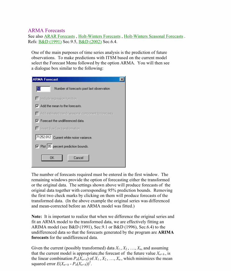
One of the main purposes of time series analysis is the prediction of futureobservations. To make predictions with ITSM based on the current modelselect the Forecast Menu followed by the option ARMA. You will then seea dialogue box similar to the following:

The number of forecasts required must be entered in the first window. Theremaining windows provide the option of forecasting either the transformedor the original data. The settings shown above will produce forecasts of theoriginal data together with corresponding 95% prediction bounds. Removingthe first two check marks by clicking on them will produce forecasts of thetransformed data. (In the above example the original series was differencedand mean-corrected before an ARMA model was fitted.)

Note: It is important to realize that when we difference the original series andfit an ARMA model to the transformed data, we are effectively fitting anARIMA model (see B&D (1991), Sec.9.1 or B&D (1996), Sec.6.4) to theundifferenced data so that the forecasts generated by the program are ARIMAforecasts for the undifferenced data.

Given the current (possibly transformed) data X1 , X2 , …, Xn, and assumingthat the current model is appropriate,the forecast of the future value Xn+h , isthe linear combination Pn(Xn+h) of X1 , X2 , …, Xn , which minimizes the meansquared error E(Xn+h - Pn(Xn+h))2.

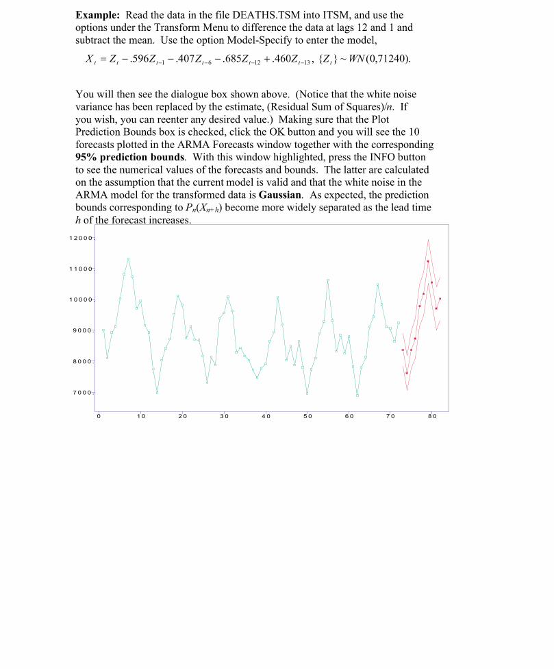
Example: Read the data in the file DEATHS.TSM into ITSM, and use theoptions under the Transform Menu to difference the data at lags 12 and 1 andsubtract the mean. Use the option Model-Specify to enter the model, ).71240,0(~}{,460.685.407.596. 131261 WNZZZZZZX ttttttt

You will then see the dialogue box shown above. (Notice that the white noise

Given the current (possibly transformed) data X1 , X2 , …, Xn, and assumingthat the current model is appropriate,the forecast of the future value Xn+h , isthe linear combination Pn(Xn+h) of X1 , X2 , …, Xn , which minimizes the meansquared error E(Xn+h - Pn(Xn+h))2.

Example: Read the data in the file DEATHS.TSM into ITSM, and use theoptions under the Transform Menu to difference the data at lags 12 and 1 andsubtract the mean. Use the option Model-Specify to enter the model,

).71240,0(~}{,460.685.407.596. 131261 WNZZZZZZX ttttttt

You will then see the dialogue box shown above. (Notice that the white noisevariance has been replaced by the estimate, (Residual Sum of Squares)/n. Ifyou wish, you can reenter any desired value.) Making sure that the PlotPrediction Bounds box is checked, click the OK button and you will see the 10forecasts plotted in the ARMA Forecasts window together with the corresponding95% prediction bounds. With this window highlighted, press the INFO buttonto see the numerical values of the forecasts and bounds. The latter are calculatedon the assumption that the current model is valid and that the white noise in theARMA model for the transformed data is Gaussian. As expected, the predictionbounds corresponding to Pn(Xn+h) become more widely separated as the lead timeh of the forecast increases.

7 0 0 0 .

8 0 0 0 .

9 0 0 0 .

1 0 0 0 0 .

1 1 0 0 0 .

1 2 0 0 0 .

0 1 0 2 0 3 0 4 0 5 0 6 0 7 0 8 0

AutofitRef: B&D (2002)., Appendix D.3.1.

Once the univariate data file in ITSM is judged to be representable by a stationary time series model, a search for a suitable model, based on minimizing the AICC criterion can be carried out as follows.Select Model>Estimation>Autofit. A dialog box will appear in which you must specify upper and lower limits for the autoregressive and moving average orders p and q. Once these limits have been specified click on Start and the search will begin.You can watch the progress of the search in the dialog box which continually updates the values of p and q and records the best model found so far.Once the search has been completed, click on Close and the current model for the data will be the one selected by Autofit.This option does not consider models in which the coefficients are required to satisfy constraints(other than causality) and consequently does not always lead to the optimal representation of the data.Since the number of maximum-likelihood models to be fitted is the product of the number of p-values and the number of q values, some care should be exercised (depending on the speed of your computer) in specifying the ranges. The maximum values for p and q are 27.

Box-Cox TransformationsSee also Classical Decomposition , Differencing , Refs: B&D (1991) p.284. , B&D (2002) Section 6.2.

These transformations can be applied to the data by selecting theoption Box-Cox from the Transform Menu. If the original data areY1, Y2 ,…, the Box-Cox transformation f converts them to f(Y1 ),f(Y2 ),…, where

.0),log(

,0,1)(

y

yyf

Such a transformation is useful when the variability of the data increasesor decreases with the level. By suitable choice of , the variability canoften be made nearly constant. In particular for positive data whosestandard deviation increases linearly with level, the variability can bestabilized by choosing = 0.

The choice of can be made visually by clicking on the pointer in thedialogue box shown below and dragging it in either direction along thescale. As the pointer is moved, the graph of the data will be seen to changewith . Once you are satisfied that the variability has been satisfactorilystabilized, leave the pointer at the chosen point on the scale and click OK.Once the transformation has been made, it can be undone using the Undosuboption of the Transform Menu. Very often it will be found that notransformation is needed or that the choice = 0 is satisfactory..

Example: Read the data file AIRPASS.TSM into ITSM. The variabilityof the data will be seen to increase with level. After selecting the Box-Coxsuboption of the Transform Menu, you will see the Box-Cox dialogue box.Clicking on the pointer and dragging it along the scale, you will find thatthe amplitude of the variability appears to stabilize for = 0. The dialoguebox and the transformed data will then appear as follows.

6.00

6.20

6.40

6.60

4.60

4.80

5.00

5.20

5.40

5.60

5.80

6.00

6.20

6.40

6.60

0 20 40 60 80 100 120 140

Burg ModelSee also Yule-Walker Model, Preliminary EstimationRefs: R.H. Jones in Applied Time Series Analysis, ed. D.F.Findley, Academic Press, 1978, B&D (2002) Section 7.6.

The multivariate Burg algorithm (see Jones (1978)) fits a (stationary) multivariate autoregression (VAR(p)) of any order p up to 20 to an m-variate series {X(t)} (where m<6). It can also automatically choose the value of p which minimizes the AICC statistic. Forecasting and simulation with the fitted model can be carried out.

The fitted model is),()()1()0()( 1 tZptXtXtX p

where the first term on the right is an m x 1-vector, the coefficients are m x m matrices and {Z(t)}~ WN(0, ).

The data (which must be arranged in m columns, one for each component) is imported to ITSM using the commands File>Project>Open>Multivariate OK and then selecting the name of the file containing the data. Click on the Plot sample cross-correlations button to check the sample autocorrelations of the component series and the cross-correlations between them. If the series appears to be non-stationary, differencing can be carried out by selecting Transform>Difference and specifying the required lag (or lags if more than one differencing operation is required). The same differencing operations are applied to all components of the series. Transform>Subtract Mean will subtract the mean vector from the series. If the mean is not subtracted it will be estimated in the fitted model and the vector .in the fitted model will be non-zero. Whether or not differencing operations and/or mean correction are applied to the series, forecasts can be obtained for the original m-variate series.

Example: Import the bivariate series LS2.TSM by selecting File>Project>Open>Multivariate,OK and then typing LS2.TSM, entering 2 for the number of columns and clicking OK. You will see the graphs of the component series as below.

9 . 5 0

1 0 . 0 0

1 0 . 5 0

1 1 . 0 0

1 1 . 5 0

1 2 . 0 0

1 2 . 5 0

1 3 . 0 0

1 3 . 5 0

1 4 . 0 0

0 2 0 4 0 6 0 8 0 1 0 0 1 2 0 1 4 0

Series 1

2 0 0 .

2 1 0 .

2 2 0 .

2 3 0 .

2 4 0 .

2 5 0 .

2 6 0 .

0 2 0 4 0 6 0 8 0 1 0 0 1 2 0 1 4 0

Series 2

These graphs strongly suggest the need for differencing. This is confirmed by inspection of the cross-correlations below, which are obtained by pressing the yellow Plot sample cross-correlations button.

-1.00

-.80

-.60

-.40

-.20

.00

.20

.40

.60

.80

1.00

0 2 4 6 8 10 12 14 16 18 20

Series 1

-1.00

-.80

-.60

-.40

-.20

.00

.20

.40

.60

.80

1.00

0 2 4 6 8 10 12 14 16 18 20

Series 1 x Series 2

-1.00

-.80

-.60

-.40

-.20

.00

.20

.40

.60

.80

1.00

0 2 4 6 8 10 12 14 16 18 20

Series 2 x Series 1

-1.00

-.80

-.60

-.40

-.20

.00

.20

.40

.60

.80

1.00

0 2 4 6 8 10 12 14 16 18 20

Series 2

The graphs on the diagonal are the sample ACF’s of Series 1 and Series 2, the top right graph shows the sample cross-correlations between Series 1 at time t+h and Series 2 at time t, for h=0,1,2,…, while the bottom left graph shows the sample cross-correlations between Series 2 at time t+h and Series 1 at time t, for h=0,1,2,…,

If we difference once at lag one by selecting Transform>Difference and clicking OK, we get the

differenced buvariate series with corresponding rapidly decaying correlation functions as shown.

- .80

- .60

- .40

- .20

. 0 0

. 2 0

. 4 0

. 6 0

. 8 0

0 2 0 4 0 6 0 8 0 1 0 0 1 2 0 1 4 0

Series 1

-3.

-2 .

-1 .

0 .

1 .

2 .

3 .

4 .

5 .

0 2 0 4 0 6 0 8 0 1 0 0 1 2 0 1 4 0

Series 2

-1.00

-.80

-.60

-.40

-.20

.00

.20

.40

.60

.80

1.00

0 2 4 6 8 10 12 14 16 18 20

Series 1

-1.00

-.80

-.60

-.40

-.20

.00

.20

.40

.60

.80

1.00

0 2 4 6 8 10 12 14 16 18 20

Series 1 x Series 2

-1.00

-.80

-.60

-.40

-.20

.00

.20

.40

.60

.80

1.00

0 2 4 6 8 10 12 14 16 18 20

Series 2 x Series 1

-1.00

-.80

-.60

-.40

-.20

.00

.20

.40

.60

.80

1.00

0 2 4 6 8 10 12 14 16 18 20

Series 2

Now that we have an apparently stationary bivariate series, we can fit an autoregression using Burg’s algorithm by simply selecting AR Model>Estimation>Burg, placing a check mark in the Minimum AICC box and clicking OK. The algorithm selects and prints out the following VAR(8) model.

========================================ITSM2000:(Multivariate Burg Estimates)========================================

Optimal value of p = 8

PHI(0).029616.033687

PHI(1)-.506793 .104381-.041950 -.496067

PHI(2)-.166958 -.014231.030987 -.201480

PHI(3)-.067112 .0593654.747760 -.096428

PHI(4)-.410820 .0786015.843367 -.054611

PHI(5)-.253331 .0488505.054576 .199001

PHI(6)-.415584 -.1280624.148542 .234237

PHI(7)-.738879 -.0150953.234497 -.005907

PHI(8)-.683868 .0254891.519817 .012280

Burg White Noise Covariance Matrix, V.071670 -.001148

-.001148 .042355

AICC = 56.318690

Model Checking: The components of the bivariate residual series can be plotted by selecting AR Model>Residual Analysis>Plot Residuals and their sample correlations by selecting AR Model>Residual Analysis>Plot Cross-correlations. The latter gives the graphs,

-1.00

-.80

-.60

-.40

-.20

.00

.20

.40

.60

.80

1.00

0 2 4 6 8 10 12 14 16 18 20

Series 1

-1.00

-.80

-.60

-.40

-.20

.00

.20

.40

.60

.80

1.00

0 2 4 6 8 10 12 14 16 18 20

Series 1 x Series 2

-1.00

-.80

-.60

-.40

-.20

.00

.20

.40

.60

.80

1.00

0 2 4 6 8 10 12 14 16 18 20

Series 2 x Series 1

-1.00

-.80

-.60

-.40

-.20

.00

.20

.40

.60

.80

1.00

0 2 4 6 8 10 12 14 16 18 20

Series 2

showing that both the auto- and cross-correlations at lags greater than zero are negligible, as they should be for a good model.

Prediction: To forecast 20 future values of the two series using the fitted model select Forecasting>AR Model, then enter 20 for the number of forecasts, retain the default Undifference Data and check the box for 95% prediction bounds. Click OK and you will then see the following predictors and bounds.

10.

11 .

12 .

13 .

14 .

15 .

16 .

0 20 40 60 80 100 120 140 160

S e r i e s 1

200.

220.

240.

260.

280.

300.

0 20 40 60 80 100 120 140 160

S e r i e s 2

Further details on multivariate autoregression can be found in B&D (1991) p. 432 and B&D (2002) Section 7.6.

Classical DecompositionSee also Box-Cox, Differencing . Refs: B&D (1991) pp.14, 284. , B&D (2002) Sections 1.5,6.2.

Classical decomposition of the series {Xt} is based on the model,,tttt YsmX

where Xt is the observation at time t , mt is a 'trend component', st , is a'seasonal component' and Yt is a 'random noise component' which isstationary with mean zero. The objective is to estimate the components mtand st and subtract them from the data to generate a sequence of residuals(or estimated noise) which can then be modelled as a stationary time series.

To carry out a classical decomposition of the data, select the option Classicalfrom the Transform Menu. You will then see the Classical DecompositionDialogue Box. In this box you must specify whether you wish to estimatetrend only, the seasonal component only or both simultaneously. Once therequired entries have been completed, click on Show Fit to check for thegoodness of the fit and then OK to complete the decomposition.

Example: Under the heading Box-Cox we showed how to stabilize thevariability of the series AIRPASS.TSM by taking logarithms. The resultingtransformed series has an apparent seasonal component of period 12(correspoonding to the month of the year) and an approximately linear trend.These can be removed by making the following entries in the ClassicalDialogue Box and then clicking Show Fit to see how the fitted trend andSeasonal components match the data. They are plotted together in a windowlabelled CLASSICAL FIT. If you are satisfied with the fit, press OK.

The effect is to transform the data to the residuals from the fitted trend andseasonal components. These are plotted on the screen in the window labelled

The effect is to transform the data to the residuals from the fitted trend andseasonal components. These are plotted on the screen in the window labelledAIRPASS.TSM and show no obvious deviations from stationarity. It is nowreasonable to attempt to fit a stationary time series model to this series.Information concerning the residual series (sample mean etc.) can be obtainedby pressing the INFO button on the toolbar at the top of the screen while thewindow labelled AIRPASS.TSM is highlighted.

To see the estimated parameter values of the trend and seasonal components,highlight the window labelled CLASSICAL FIT and press the INFO button onthe toolbar at the top of the screen.

Instead of fitting the most general seasonal component, it is also possible tofit a polynomial trend plus a finite linear combination of sinusoidalcomponents by checking Harmonic Regression instead of Seasonal Fit inthe Classical Dialogue Box. For details see B&D(1996), pp. 12,13.

Color Customization

The colors of the displayed graphs can be chosen by right-clicking on a graph and selecting the option Customize Colors. The following dialog box will then appear.

To select the graphs for which the color is to be assigned, select one of the numbers 1 through 25 and click on Choose Color. The following palette will then appear.

Select your color and click on OK. All of the graphs corresponding to the number you selected in the Customize Colors dialog box will then be set to the chosen color. The graphs corresponding to each of the numbers 1 through 25 are listed below.

Color Map:Plot 1:

tsplot of dataqqplotsample acf of time seriesspectral estimatesestimated cumulative spectrumhistogramoriginal data in classical decomposition plotSeries 1 for multivariate projectssample acf of transfer function residuals

Plot 2:model acfmodel spectrummodel cumulative spectrumclassical fitpredicted valuessmoothed valuesSeries 2 for multivariate projects

Plot 3:tsplot of residualsqqplot of residualssample acf of residualshistogram of residualssample acf of abs values of residualsSeries 3 for multivariate projects

Plot 4:tsplot of stochastic volatilityqqplot of garch residualssample acf of abs values of garch residualsSeries 4 for multivariate projects

Plot 5:sample pacf of time seriesstandardized spectral estimateSeries 5 for multivariate projects

Plot 6:model pacfprediction boundsSeries 6 for multivariate data

Plot 7:sample pacf of residualssample acf of squared values of residualsSeries 7 for multivariate projects

Plot 8:sample acf of squares of garch residualsSeries 8 for multivariate projects

Plot 9:Series 9 for multivariate projects

Plot 10: Series 10 for multivariate projects



Constrained MLESee also Maximum Likelihood Estimation , Preliminary Estimation , Refs: B&D (1991) p.324 , B&D (2002) Section 6.5.

The time series models fitted to data frequently have coefficients which aresubject to constraints. For example the multiplicative seasonal ARMA model,

s)Xt = sZt ,where and are polynomials of orders p, q, P and Q respectively,can be expressed as an ARMA(u, v) model where

u = p + sP and v = q + sQ(see B&D (1991), p.323 or B&D (1996), p.201). However the coefficientsin the ARMA(u,v) model satisfy a number of multiplicative constraintsdetermined by the multiplicative form of the autoregressive and moving averagepolynomials. Another important class of constrained models are those in whichparticular ARMA coefficients are constrained to be zero (or some other value).Such constraints are handled by ITSM using the option Model-Estimation-MaxLikelihood see (Maximum Likelihood Estimation) and pressing the ConstrainOptimization Button. You will then see the dialogue box of the following formwhich will be explained with reference to the following example.

Example: The data in the file DEATHS.TSM were differenced at lags 12 and 1 toremove trend and seasonality and then mean-corrected. The sample ACF of theresulting series has large autocorrelations at lags 1 and 12 and small ones (compared)with 1.96n -1/2 ) at other lags. This suggests two possible models, an MA(12) of theform,(1) Xt = Zt +Zt -12 ,or a multiplicative MA(13) of the form,(2) Xt = (1 + + 12) = Zt +Zt -12+where, in the latter model the coefficients satisfy the multiplicative constraint,(3) 13 = 12

To investigate these two potential models we first fit a preliminary MA(13) model

remove trend and seasonality and then mean-corrected. The sample ACF of theresulting series has large autocorrelations at lags 1 and 12 and small ones (compared)with 1.96n -1/2 ) at other lags. This suggests two possible models, an MA(12) of theform,(1) Xt = Zt +Zt -12 ,or a multiplicative MA(13) of the form,(2) Xt = (1 + + 12) = Zt +Zt -12+where, in the latter model the coefficients satisfy the multiplicative constraint,(3) 13 = 12

To investigate these two potential models we first fit a preliminary MA(13) modelby selecting the option Model-Estimation-Preliminary-Innovations with the AR orderset to 0 and the MA order set to 13. Then selecting Model-Estimation-Max Likelihoodand pressing the Constrain Optimization button we obtain precisely the dialogue boxshown above.

To fit Model (1), highlight each of the coefficients , … ,and , and press thebutton Set to Zero. You will see these coefficients revert to zero in the dialogue box.Then press OK and you will return to the Maximum Likelihood Estimation DialogueBox. Press OK again and you will see the fitted model, with AICC value 856.04.

To fit Model (2), again starting from the dialogue box shown above, set thecoefficients with subscripts from 2 to 11 equal to zero as in (2). Then enter 1 in thewindow labelled Number of Relations and on the line below,

1 x 12 = 13to indicate the constraint (3). Check also that MA is indicated. Then press OK andyou will return to the Maximum Likelihood Dialogue Box. Press OK again and youwill see the fitted model, with AICC value 857.36.

Cross-correlationsSee also Cross-spectrum, Burg Model, Yule-Walker Model and Transfer Function ModellingRefs: B&D (1991) p.406, B&D (2002) Section 7.2.

The sample cross-correlation functions of the component series,)}({)},({)},({ 21 tYtYtY m

of an m-variate time series observed at times t=1,…,n, are defined as follows:,||,)]0()0()[()( 2/1

,,,, nhhh jjiijiji where

,0],)(][)([)(1

1,

hYtYYhtYnh jji

hn

t ijiand

.0],)(][)([)(1

1,

hYtYYhtYnh jjin

ht ijiObserve that

).()( ,, hh ijji

Example: The time series DJAO2.TSM consists of 251 successive daily closing prices of the Dow-Jones Industrial Average (Series 1) and the Australian All-ordinaries Index (Series 2). Import the bivariate series into ITSM by selecting File>Project>Open>Multivariate, then click OK, type DJAO2.TSM and specify 2 columns in the dialog box which appears. Choose Transform>Difference and select lag 1 to get the bivariate series whose components are plotted below.

- 1 0 0 .

- 8 0 .

- 6 0 .

- 4 0 .

- 2 0 .

0 .

2 0 .

4 0 .

6 0 .

8 0 .

0 5 0 1 0 0 1 5 0 2 0 0 2 5 0

Series 1

- 6 0 .

- 4 0 .

- 2 0 .

0 .

2 0 .

4 0 .

6 0 .

0 5 0 1 0 0 1 5 0 2 0 0 2 5 0

Series 2

Press the yellow Plot sample autocorrelations button and you will see the array of autocorrelation and cross-correlation functions shown belowNote: The convention in plotting the array of cross-correlations is that the jth graph in the ith

row is the estimated correlation of the ith series at time t+h with the jth series at time t, for h=0,1,2,…. For example the graphs below show that there is a significant correlation between the differenced Series 2 (All-ordinaries Index) at time t+1 and the differenced Series 1 (Dow-Jones Index) at time t. This demonstrates a tendency of increments of the Australian All-ordinaries Index to follow those of the Dow-Jones Index by one day.

-1.00

-.80

-.60

-.40

-.20

.00

.20

.40

.60

.80

1.00

0 2 4 6 8 10 12 14 16 18 20

Series 1

-1.00

-.80

-.60

-.40

-.20

.00

.20

.40

.60

.80

1.00

0 2 4 6 8 10 12 14 16 18 20

Series 1 x Series 2

-1.00

-.80

-.60

-.40

-.20

.00

.20

.40

.60

.80

1.00

0 2 4 6 8 10 12 14 16 18 20

Series 2 x Series 1

-1.00

-.80

-.60

-.40

-.20

.00

.20

.40

.60

.80

1.00

0 2 4 6 8 10 12 14 16 18 20

Series 2

Further details on cross-correlations can be found in B&D (1991) p.406 and B&D (2002)Section 7.2.

Cross-correlationsSee also Cross-spectrum, Burg Model, Yule-Walker Model and Transfer Function ModellingRefs: B&D (1991) p.406, B&D (2002) Section 7.2.

The sample cross-correlation functions of the component series,)}({)},({)},({ 21 tYtYtY m

of an m-variate time series observed at times t=1,…,n, are defined as follows:,||,)]0()0()[()( 2/1

,,,, nhhh jjiijiji where

,0],)(][)([)(1

1,

hYtYYhtYnh jji

hn

t ijiand

.0],)(][)([)(1

1,

hYtYYhtYnh jjin

ht ijiObserve that

).()( ,, hh ijji

Example: The time series DJAO2.TSM consists of 251 successive daily closing prices of the Dow-Jones Industrial Average (Series 1) and the Australian All-ordinaries Index (Series 2). Import the bivariate series into ITSM by selecting File>Project>Open>Multivariate, then click OK, type DJAO2.TSM and specify 2 columns in the dialog box which appears. Choose Transform>Difference and select lag 1 to get the bivariate series whose components are plotted below.

- 1 0 0 .

- 8 0 .

- 6 0 .

- 4 0 .

- 2 0 .

0 .

2 0 .

4 0 .

6 0 .

8 0 .

0 5 0 1 0 0 1 5 0 2 0 0 2 5 0

Series 1

- 6 0 .

- 4 0 .

- 2 0 .

0 .

2 0 .

4 0 .

6 0 .

0 5 0 1 0 0 1 5 0 2 0 0 2 5 0

Series 2

Press the yellow Plot sample autocorrelations button and you will see the array of autocorrelation and cross-correlation functions shown belowNote: The convention in plotting the array of cross-correlations is that the jth graph in the ith

row is the estimated correlation of the ith series at time t+h with the jth series at time t, for h=0,1,2,…. For example the graphs below show that there is a significant correlation between the differenced Series 2 (All-ordinaries Index) at time t+1 and the differenced Series 1 (Dow-Jones Index) at time t. This demonstrates a tendency of increments of the Australian All-ordinaries Index to follow those of the Dow-Jones Index by one day.

-1.00

-.80

-.60

-.40

-.20

.00

.20

.40

.60

.80

1.00

0 2 4 6 8 10 12 14 16 18 20

Series 1

-1.00

-.80

-.60

-.40

-.20

.00

.20

.40

.60

.80

1.00

0 2 4 6 8 10 12 14 16 18 20

Series 1 x Series 2

-1.00

-.80

-.60

-.40

-.20

.00

.20

.40

.60

.80

1.00

0 2 4 6 8 10 12 14 16 18 20

Series 2 x Series 1

-1.00

-.80

-.60

-.40

-.20

.00

.20

.40

.60

.80

1.00

0 2 4 6 8 10 12 14 16 18 20

Series 2

Further details on cross-correlations can be found in B&D (1991) p.406 and B&D (2002)Section 7.2.

Cross-spectrumSee also Cross-correlations , Burg Model and Yule-Walker Model .Ref: B&D (1991) p.434.

The spectral density matrix of a multivariate stationary time series {X(t) , t = 0, 1, . . .}with absolutely summable matrix covariance function (in particular of a multivariate ARMA process) can be expressed as

,,)()2()( 1

ki

kekf

where = 1 . The spectral decomposition of {X(t)} breaks it into sinusoidal components; f() d is the contribution to the covariance matrix of X(t) from components with frequencies in (dwhere is measured in radians per unit time. The ith diagonal component of the spectral density matrix is just the spectral density of the ith component series. The (i,j)-component of the spectral density matrix is called the cross-spectral density of the ith and jth component series and is complex when i and j are not equal.

The spectral density matrix can be estimated (but not consistently) by 1/() times the multivariate periodogram, defined at the Fourier frequency 2j/n (where n is the number of observation vectors) by

.)()()(*

111

n

t

itn

t

itj

jj etXetXnI The superscript * denotes complex conjugate transpose. If we have a multivariate project in ITSM, then selecting the options Statistics>Cross Spectrum will produce an array of graphs. The ith diagonal graph is the periodogram estimate of the spectral density of the ith component series, i.e. the function,

.0),2/()( jjiiIThe graph in the (i,j)-location above the diagonal is the corresponding estimate of the phase spectrum i,j) and the graph in the (i,j)-location below the diagonal is the estimate of the squared coherency |i,j)|2. See B&D (1991) p.436 for the definitions of these quantities.

As in the univariate case, good estimates of the spectral density, phase spectrum and squared coherency can only be obtained by smoothing the multivariate periodogram defined in the preceding paragraph. The smoothed periodogram estimate of the spectral density matrix at the Fourier frequency j is

),()(21)(ˆ

m

mk kjj IkWf

where the weights W(k) are non-negative, add to 1 and satisfy W(k) = W(-k). They are chosen by selecting Statistics>Smooth Spectrum. You will then see a dialog box. If you select, for example, two Daniell filters, one of order 3 and the second of order 5, it will appears as follows:

The weights pictured in the dialog box are generated by the successive application of n(=2) Daniell filters (filters with W(k) = 1/(2m+1), k= -m, . . . , m, where m is the order of the filter; 3 for the first and 5 for the second in the above example). Clicking OK will produce graphs of the estimated spectral densities, phase spectra and squared coherencies based on the corresponding smoothed periodogram estimate of the matrix spectral density function

Example: Import the project LS2.TSM by selecting File>Project>Open>Multivariate, OK and then typing LS2.TSM, entering 2 for the number of columns and again clicking OK. Select Transform>Difference and Lag 1 to generate a stationary-looking bivariate series.

Select Statistics>Cross-spectrum and you will see the following multivariate periodogram estimates.

.000

.020

.040

.060

.080

.100

.120

.140

.0 .5 1.0 1.5 2.0 2.5 3.0

Periodogram: Series 1

-3.

-2.

-1.

0.

1.

2.

3.

.0 .5 1.0 1.5 2.0 2.5 3.0

Phase: Series 1 x Series 2

10.E+00

10.E+00

10.E+00

1.0E+00

1.0E+00

1.0E+00

1.0E+00

.0 .5 1.0 1.5 2.0 2.5 3.0

Sq. Coherence: Series 1 x Series 2

.00

.50

1.00

1.50

2.00

2.50

3.00

3.50

4.00

.0 .5 1.0 1.5 2.0 2.5 3.0


Select Statistics>Smooth spectrum ,complete the dialog box as above, click OK and you will see the improved estimates,

.0000

.0050

.0100

.0150

.0200

.0250

.0300

.0350

.0400

.0450

.0 .5 1.0 1.5 2.0 2.5 3.0


-3.

-2.

-1.

0.

1.

2.

3.

.0 .5 1.0 1.5 2.0 2.5 3.0

Phase: Series 1 x Series 2

.650

.700

.750

.800

.850

.900

.950

.0 .5 1.0 1.5 2.0 2.5 3.0

Sq. Coherence: Series 1 x Series 2

.20

.40

.60

.80

1.00

1.20

.0 .5 1.0 1.5 2.0 2.5 3.0


The diagonal graphs indicate that the differenced Leading Indicator series (Series 1) has a predominance of high frequency components in its spectral decomposition while the differenced Sales series has a predominance of low frequency components. The estimated squared coherency (bottom left) indicates that the high-frequency components of the two series are more strongly linearly related than the low frequency components. The estimated phase spectrum (top

right) has an approximately constant slope of three, indicating that all the frequency components of the Leading Indicator series lead those of the Sales series by approximately three days. It is interesting to compare this interpretation with the transfer-function model for the same bivariate series.

Further details on cross-spectra can be found in B&D (1991) p.434.

DATA SETSSee also GETTING STARTED , TSM Files , Refs: B&D (1991), B&D (2002).

AIRPASS.TSM International airline passenger monthly totals (in thousands), Jan. 49 -- Dec. 60. From Box and Jenkins (Time Series Analysis: Forecasting and Control, 1970). B&D (1991)Example 9.2.2. B&D (2002) Example. 8.5.2

APPA.TSM Lake level of Lake Huron in feet (reduced by 570), 1875--1972. B&D (1991)Appendix Series A. B&D (2002) Example 1.3.5

APPB.TSM Dow Jones Utilities Index, Aug.28--Dec.18, 1972. B&D (1991) Appendix Series B. B&D (2002) Example 5.1.5

APPC.TSM Private Housing Units Started, U.S.A. (monthly). From the Makridakis competition, series 922. B&D (1991) Appendix Series C.

APPD.TSM Industrial Production, Austria (quarterly). From the Makridakis competition, Series 337. B&D (1991) Appendix Series D.

APPE.TSM Industrial Production, Spain (monthly). From the Makridakis competition, Series 868. B&D (1991) Appendix Series E.

APPF.TSM General Index of Industrial Production (monthly). From the Makridakis competition, Series 904. B&D (1991) Appendix, Series F.

APPG.TSM} Annual Canadian Lynx Trappings, 1821--1934. B&D (1991) Appendix Series G.

APPH.TSM Annual Mink Trappings, 1848--1911. B&D (1991) Appendix Series H.

APPI.TSM Annual Muskrat Trappings, 1848--1911. B&D (1991) Appendix Series I. B&D (2002) Problem 7.8

APPJ.TSM Simulated input series for transfer function model. B&D (1991) Appendix Series J. B&D (2002) Problem 7.7

APPK.TSM Simulated output series for transfer function model. B&D (1991) Appendix Series K. . B&D (2002) Problem 7.7

APPJK2.TSM The two series APPJ and APPK (see above) in bivariate format. . B&D (2002)Problem 7.7

ARCH.TSM 1000 simulated values of an ARCH(1) process. B&D (2002) Example 10.3.1.

BEER.TSM Australian monthly beer production in megalitres,including ale and stout and

excluding beverages with alcoholpercentage less than 1.15. January, 1956, through April, 1990 (Australian Bureau of Statistics). B&D (2002) Problem 6.10.

CHAOS.TSM The series x(t), t=1,…,200, defined by the logistic equation x(t)=4x(t-1)[1-x(t-1)] with x(0)=/10. B&D (2002) Section 10.3.2.

CHOCS.TSM Australian monthly chocolate-based confectionery production in tonnes. July, 1957, through October, 1990 (Australian Bureau of Statistics).

DEATHS.TSM Monthly accidental deaths in the U.S.A., 1973— 1978 (National Safety Council). B&D (1991) Example 1.1.6. B&D (2002) Example 1.1.3.

DJAO2.TSM Closing daily values of the Dow-Jones Industrial Index and of the Australian All-ordinaries Stock Index for 251 successive trading days, ending August 26th, 1994 (stored in bivariate format). B&D (2002) Example 7.1.1.

DJAOPC2.TSM Daily percentage changes (250 values) obtained from DJAOPC.TSM (stored in bivariate format). B&D (2002) Example 7.1.1.

DJAOPCF2.TSM Observed daily values of the percentage changes in the Dow-Jones Industrial Index and the Australian All-ordinaries Stock Index for the forty days following the data in DJAOPC2.TSM (stored in bivariate format). B&D (2002) Example 7.6.3.

DOWJ.TSM Dow-Jones Utilities Index. Same as APPB.TSM above. B&D (2002) Example 5.1.5.

E1021.TSM Sinusoid plus simulated Gaussian white noise. B&D (1991) Example 10.2.1.

E1032.TSM Observed percentage daily returns on the Dow-Jones Industrial Index for the period July 1st, 1997 through April 9th, 1999. B&D (2002) Example 10.3.2.

E1042.TSM 160 simulated values of an MA(1) process. B&D (1991) Example 10.4.2.

E1062.TSM 400 simulated values of an MA(1) process. B&D (1991) Example 10.6.2.

E1321.TSM 200 values of a simulated fractionally differenced MA(1) series.B&D (1991)Example 13.2.1.

E1331.TSM 200 values of a simulated MA(1) series with standard Cauchy white noise.B&D (1991) Example 13.3.2.

E1332.TSM 200 values of a simulated AR(1) series with standard Cauchy white noise.B&D (1991) Example 13.3.2.

E334.TSM 10 simulated values of an ARMA(2,3) process. B&D (1991) Example 5.3.4, B&D

(2002)Example 3.3.4.

E611.TSM 200 simulated values of an ARIMA(1,1,0) process. B&D (1991) Example 9.1.1, B&D (2002)Example 6.1.1.

E731A.TSM 200 simulated values of a bivariate series whose components are independent AR(1) processes, each with coefficient 0.8 and white-noise variance 1. B&D (2002)Example 7.3.1.

E731B.TSM Bivariate residual series obtained after fitting AR(1) models to each of the component series stored in the file E731A.TSM. B&D (2002)Example 7.3.1.

E732.TSM Bivariate residual series obtained after fitting the models (7.1.1) and (7.1.2) respectively to the series {D(t,1)} and {D(t,2)} of Example 7.1.1. B&D (2002)Examples 7.1.1, 7.3.2..

E921.TSM 200 simulated values of an AR(2) process. B&D (1991) Example 9.2.1.

E923.TSM 200 simulated values of an ARMA(2,1) process. B&D (1991) Example 9.2.3.

E951.TSM 200 simulated values of an ARIMA(1,2,1) process. B&D (1991) Example 9.5.1.

ELEC.TSM Australian monthly electricity production in millions of kilowatt hours. January, 1956, through April, 1990 (Australian Bureau of Statistics).

FINSERV.TSM Australian expenditure on financial services in millions of dollars. September quarter, 1969, through March quarter, 1990 (Australian Bureau of Statistics).

GNFP.TSM Australian gross non-farm product at average 1984/5 prices in millions of dollars. September quarter, 1959, through March quarter, 1990 (Australian Bureau of Statistics).

GOALS.TSM Soccer goals scored by England in matches against Scotland at Hampden Park in Glasgow, 1872-1987. B&D (2002)Example 8.8.7.

IMPORTS.TSM Australian imports of all goods and services in millions of Australian dollars at average 1984/85 prices. September quarter, 1959, through December quarter, 1990 (Australian Bureau of Statistics).

LAKE.TSM Lake level of Lake Huron in feet (reduced by 570), 1875--1972. B&D (1991)Appendix Series A. B&D (2002) Example 1.3.5

LEAD.TSM Leading Indicator Series from Box and Jenkins (Time Series Analysis: Forecasting and Control, 1970). B&D (1991) Example 11.2.2. B&D (2002)Example 10.1.1.

LRES.TSM Whitened Leading Indicator Series obtained by fitting an MA(1) to the

mean-corrected differenced series LEAD.TSM. B&D (1991) Section 13.1. B&D (2002)Example 10.1.1.

LS2.TSM The two series LEAD and SALES (see above) in bivariate format. B&D (2002)Example 10.1.1.

LYNX.TSM Annual Canadian Lynx Trappings, 1821--1934. B&D (1991) Appendix Series G.

NILE.TSM Minimal yearly water levels of the Nile River as measured at the Roda gauge near Cairo for the years 622—871. (Source: http://lib.stat.cmu.edu/S/beran.) B&D (2002) Example 10.5.1.

OSHORTS 57 consecutive daily overshorts from an undergraound gasoline tank at a filling station in Colorado. B&D (2002)Example 3.2.8.

POLIO.TSM Monthly numbers of newly recorded polio cases in the U.S.A., 1970-1983. B&D (2002)Example 8.8.3

SALES.TSM Sales Data from Box and Jenkins (Time Series Analysis: Forecasting and Control, 1970). B&D (1991) Example 11.2.2. B&D (2002)Example 10.1.1.

SBL.TSM The number of car drivers killed or seriously injured monthly in Great Britain for ten years beginning in January 1975 B&D (2002) Examples 6.6.3 and 10.2.1.

SBLD.TSM The number of car drivers killed or seriously injured monthly in Great Britain for ten years beginning in January 1975 after differencing at lag 12. B&D (2002) Examples 6.6.3 and 10.2.1.

SBLIN.TSM The step-function regressor, f(t)=0 for 0<t<99, and f(t)=1 for 98<t<121, to account for seat-belt legislation in B&D (2002) Examples 6.6.3 and 10.2.1.

SBLIND.TSM The function g(t) obtained by differencing the function f(t) of SBLIN.TSM at lag 12. B&D (2002) Examples 6.6.3 and 10.2.1.

SBL2.TSM The bivariate series ose first components are the data in SBLIN.TSM and whose second components are the data in SBL.TSM. B&D (2002) Example 10.2.1.

SIGNAL.TSM Simulated vales of the series X(t)=cos(t) +N(t), t=0.1,0.2,…,20.0, where N(t) is WN(0,0.25). B&D (2002)Example 1.1.4.

SRES.TSM Residuals obtained from the mean-corrected and differenced SALES.TSM data when the filter used for whitening the mean-corrected differenced LEAD.TSM series is applied. B&D (1991) Section 13.1. B&D (2002)Example 10.1.1.

STOCK7.TSM Daily returns (100ln(P(t)/P(t-1))) based on closing prices P(t) of 7 stock indices

871. (Source: http://lib.stat.cmu.edu/S/beran.)

in multivariate format. The first return is for April 27, 1998, and the last is for April 9, 1999. The indices are, in order: Australian All-ordinaries, Dow-Jones Industrial, Hang Seng, JSI (Indonesia), KLSE (Malaysia), Nikkei 225, KOSTI (South Korea).

STOCKLG7.TSM Longer version of STOCK7.TSM. The first return is for July 2, 1997, and the last is for April 9, 1999.

STRIKES.TSM Strikes in the U.S.A., 1951--1980 (Bureau of Labor Statistics). B&D (1991)Example 1.1.3. B&D (2002) Example 1.1.6.

SUNSPOTS.TSM The Annual sunspot numbers, 1770--1869. B&D (1991) Example 1.1.5. B&D (2002) Example 3.2.9.

USPOP.TSM Population of United States at ten-year intervals, 1790--1980 (U.S.Bureau of the Census). B&D (1991) Example 1.1.2. B&D (2002) Example 1.1.5.

WINE.TSM Monthly sales (in kilolitres) of red wine by Australian winemakers from January, 1980 through October 1991. (Australian Bureau of Statistics). B&D (2002) Example 1.1.5.

Data Transfer

Data files which can be read by ITSM are ASCII files in which univariate data are arranged in a single column and m-variate data are arranged in m columns, separated by one or more spaces,with the rows arranged in chronological order. Any ASCII text editor, e.g. Wordpad or Notepad, can be used to create such a file.

Note: When a project is saved as a .TSM file by ITSM, coded model information is saved as well as the data. Editing such files directly using a text editor is therefore not recommended.

The most convenient way to create, manipulate and transfer data to and from ITSM is to use the program in conjunction with a spreadsheet such as Excel.

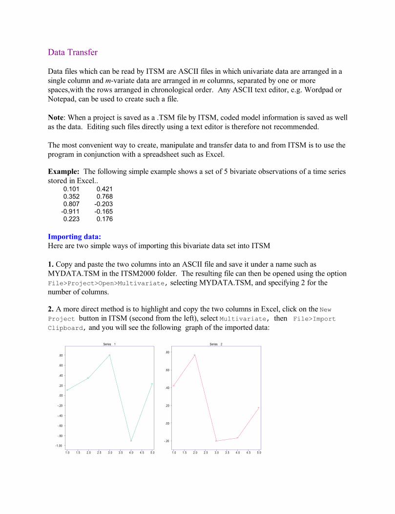
Example: The following simple example shows a set of 5 bivariate observations of a time series stored in Excel..

0.101 0.4210.352 0.7680.807 -0.203

-0.911 -0.1650.223 0.176

Importing data:Here are two simple ways of importing this bivariate data set into ITSM

1. Copy and paste the two columns into an ASCII file and save it under a name such as MYDATA.TSM in the ITSM2000 folder. The resulting file can then be opened using the option File>Project>Open>Multivariate, selecting MYDATA.TSM, and specifying 2 for the number of columns.

2. A more direct method is to highlight and copy the two columns in Excel, click on the New Project button in ITSM (second from the left), select Multivariate, then File>Import Clipboard, and you will see the following graph of the imported data:

-1.00

-.80

-.60

-.40

-.20

.00

.20

.40

.60

.80

1.0 1.5 2.0 2.5 3.0 3.5 4.0 4.5 5.0

Series 1

-.20

.00

.20

.40

.60

.80

1.0 1.5 2.0 2.5 3.0 3.5 4.0 4.5 5.0

Series 2

Exporting data:The data in ITSM (and other quantities which have been calculated, such as spectra, autocorrelation functions etc) can be exported either to a file or to the clipboard (and thence to a spreadsheet) simply by clicking on the red EXP button and selecting the data to be exported and the required destination.If the data are exported to the clipboard and pasted into a spreadsheet, they can then be manipulated or edited in the spreadsheed and read back into ITSM as described above.

DifferencingSee also Box-Cox , Classical Decomposition . Refs: B&D (1991) pp.19, 24, 274. , B&D (2002) Sections 1.5, 6.1, 6.2.

Differencing is a technique which (like Classical Decomposition) can be usedto remove seasonal components and trends. The idea is simply to considerthe differences between successive pairs of observations with appropriate timeseparations. For example, to remove a seasonal component of period 12 fromthe series {Xt} , we generate the transformed series,

,)1( 1212 tttt XBXXY

where B is the backward shift operator (i.e. B j Xt = Xt-j ). It is clear that allseasonal components of period 12 are eliminated by this transformation,which is called differencing at lag 12. A linear trend can be eliminated bydifferencing at lag 1, and a quadratic trend by differencing twice at lag 1 (i.e.differencing once to get a new series, then differencing the new series to get asecond new series). Higher-order polynomials can be eliminated analogously.It is worth noting that differencing at lag 12 not only eliminates seasonalcomponents with period 12 but also any linear trend.

Repeated differencing in PEST can be carried out using the option Differenceof the Transform Menu.

Example: Under the heading Box-Cox we showed how to stabilize thevariability of the series AIRPASS.TSM by taking logarithms. Assuming thatthis has been done, the resulting transformed series has an apparent seasonalcomponent of period 12 (corresponding to the month of the year) and anapproximately linear trend. These can both be removed by differencing at lag12. To do this select the option Difference from the Transform Menu, enter 12in the highlighted window of the dialogue box shown below and click OK. Thegraph of the differenced series will then appear in the window AIRPASS.TSM.

It shows no apparent seasonality, however there is a slight trend which suggeststhe possibility of differencing again, this time at lag 1. To do this, select theoption Difference from the Transform Menu, specify a lag equal to 1 and clickthe Ok button. The graph in the window AIRPASS.TSM will then show thetwice differenced series,

,)1)(1( 1312112

tttttt XXXXXBBYwhere {Xt} is the series of logarithms of the original data. The series {Yt} showsno apparent trend or seasonality, so it is reasonable to try and model it as astationary time series.

Exponential Smoothing

See also Moving Average Smoothing, Spectral Smoothing (FFT), Holt-Winters ForecastsRefs: B&D (1991) p.17, B&D (2002) Sections 1.5, 9.2.

After selecting the suboption Exponential Smooth from theSmooth menu, a dialogbox will open requesting you to specify avalue for the parameter a in the smoothing recursions,

( ) , ,..., .m Xm aX a m t nt t t

1 1

11 2

The choice a=1 gives no smoothing (m̂ t = Xt , tn) whilethe choice a=0 gives maximum smoothing (m̂ t = X1 , tn).Enter -1 if you would like the program to select a value for aautomatically. This option is particularly useful if you plan to usethe smoothed value m̂n as the predictor of the next observationX n+1 . The automatic selection option determines the value of awhich minimizes the sum of squares,

( )m Xjj

nj

22

of the prediction errors when each smoothed value m̂j is used as thepredictor of the next observation Xj .

Once the parameter a has been entered (or automatically selected),the program will graph the smoothed time series with the originaldata and will display the root of the average squared deviation ofthe smoothed values from the original observations defined by

SQRT(MSE) ( ) n m Xjj

nj

11

2

Fisher's TestSee also Periodogram , Cumulative Periodogram . Refs: B&D (1991) p.337, 342.

Fisher's test enables you to test the null hypothesis that the data isa realization of Gaussian white noise against the alternative that itcontains a hidden periodic component with unspecified frequency.The test statistic is defined as

q

i i

iqiq

Iq

I

11

1

)(

)(max

,

where q = [(n - 1)/2] and I(j is the periodogram at the Fourierfrequency j=j/n. f q is sufficiently large then the null hypothesisis rejected. To apply the test, select the Fisher Test suboption fromthe Spectrum Menu and the p-value of the test will be displayed. Thenull hypothesis is rejected at level if the p-value is less than .

Example: Applying the test to the series SUNSPOTS.TSM gives thefollowing result

GARCH ModelsRef: B&D (2002)., Section 10.3.5.

A GARCH(p,q) process {Zt } is a stationary solution of the equations,

,

),1,0(~}{,

1

2

10 jt

q

jjit

p

iit

t

ttt

hZh

IIDeeZ

where 2tth

and (in ITSM and most practical applications))1,0(~ Net

or

tet ~

2(Student’s t-distribution with degrees of freedom)To ensure stationarity, the coefficients are constrained to satisfy the sufficient conditions,

.1......

,0,...,,,...,,0

11

11

0

qp

qp

.An ARCH(p) process is a GARCH(p,0) process.

ESTIMATIONTo fit a GARCH model with N(0,1) noise:

Given a zero-mean or mean corrected data set {Zt } opened in ITSM (which may, for example, consist of residuals from a regression or ARMA model), a GARCH(p,q) model with N(0,1) noise, e(t), can be fitted as follows: Click on the red button labeled GAR. Specify the orders p and q, make sure that Use normal noise. is selected, and click on OK. Click on the red MLE button. In the dialog box which then appears, choose to subtract the

sample mean unless you wish to assume that the mean of the series is zero. The GARCH Maximum Likelihood Estimation dialog box will then open. Click on OK and

the program will minimize –2ln(L) with L as defined in (10.3.16) of B&D (2002). The estimated parameters and the values of –2ln(L) and the AICC statistic will then appear in the Garch ML estimates window.

Repeat the previous two steps until the parameter estimates stabilize. For order selection repeat the steps above with a variety of values for p and q, and select the

model with smallest AICC value. Model checks can be performed (a) by selecting Garch>Garch

residuals>QQ-Plot(normal) (the resulting graph should be approximately a straight line

through the origin with slope 1), and (b) by clicking on the fifth red button which plots the sample ACF of the absolute values and squares of the GARCH residuals (these should all be close to zero since the GARCH residuals should resemble an iid sequence).

To fit a GARCH model with t-distributed noise:Proceed exactly as above, but making sure that the option Use t-distribution for

noise is selected in each of the dialog boxes where it appears. For the GARCH model with t-distributed noise, the conditional likelihood L is defined by (10.3.19) in B&D (2002).

It is frequently useful , before fitting a GARCH model with t-distributed noise, to fit a model of the same order with N(0,1) noise. This has the effect of initializing the search with the coefficients estimated for the Gaussian noise model. It is also advisable to try more than one set of initial coefficients to minimize the risk of finding only a local minimum value of –2ln(L).

For financial data it is often found that a GARCH model with t-distributed noise provides a substantially better fit (in terms of AICC and model-checking criteria) than does a GARCH model with Gaussian noise.

To estimate the stochastic volatility:Once a model has been fitted to the data set {Zt}, a graph of the estimated volatility, i.e.

(t), is obtained by clicking on the red SV button.

SIMULATIONOnce a GARCH model has been specified in ITSM, simulation from the model can be carried

out by selecting the option Model>Simulate.

Example 1: (Fitting a GARCH model to stock data.) Open the file E1032 in ITSM and select {Transform>Subtract mean} to subtract the mean (.0608) from the data. You will then see the following graph of the mean-corrected daily returns on the Dow-Jones Industrial Index from July 1st 1997 through April 9th, 1999.

-8.

-6.

-4.

-2.

0 .

2 .

4 .

6 .

0 50 100 150 200 250 300 350 400 450

Series

The graph suggests that there are periods of high variability followed by periods of low volatility. The sample autocorrelation function of the data is not significantly different from zero

at lags greater than zero but the sample autocorrelations of the absolute values and squares shown below are much more significant, suggesting that a GARCH model might be appropriate for this data set.

-1.00

-.80

-.60

-.40

-.20

.00

.20

.40

.60

.80

1.00

0 5 10 15 20 25 30 35 40

Residual ACF: Abs values

-1.00

-.80

-.60

-.40

-.20

.00

.20

.40

.60

.80

1.00

0 5 10 15 20 25 30 35 40

Residual ACF: Squares

Following the steps above for fitting a GARCH(1,1) model with N(0,1) noise we obtain the following model for the mean-corrected series displayed in the Garch Maximum likelihood estimates window.

========================================ITSM::(Garch Maximum likelihood estimates)========================================ARMA Model: X(t) = Z(t)

Garch Model for Z(t): Z(t) = sqrt(h(t))e(t)h(t) = .1302292 + .1266656 Z^2(t-1)+ .7919689 h(t-1)

Alpha Coefficients.130229 .126666

Standard Error of Alpha Coefficients.048486 .019032

Beta Coefficients.791969

Standard Error of Beta Coefficients.040337

AICC(Garch) = .146902E+04-2Log(Likelihood) = .145778E+04

Now starting from this model we can fit a GARCH(1,1) model with t-distributed noise by simply clicking on the red MLE button again, selecting Use t-distribution as noise, and clicking

on OK. This gives the results,

========================================ITSM::(Garch Maximum likelihood estimates)========================================ARMA Model: X(t) = Z(t)

Garch Model for Z(t): Z(t) = sqrt(h(t)) e(t)h(t) = .1309970 + .06739304 Z^2(t-1)+ .8406119 h(t-1)

Alpha Coefficients.130997 .067393

Standard Error of Alpha Coefficients.074217 .031923



Degrees of freedom for t-dist = 5.745331 Standard Error of degrees of freedom = 1.390426

AICC(Garch) = .143788E+04-2Log(Likelihood) = .142467E+04

Note: The minimum is rather flat, so you may find small discrepancies in your estimated coefficients from those given above. It is very clear however that in terms of AICC, the GARCH(1,1) with t-distributed noise is very much superior to the GARCH(1,1) with Gaussian noise. Checking alternative values for p and q indicates that the GARCH(1,1) with t-distributed noise is the best model for the data of those in the categories considered. The sample autocorrelation functions of the absolute values and squares of the GARCH residuals are compatible with those of an iid series as required. The qq plot of the GARCH residuals based on the t-distribution with 5.475 degrees of freedom is reasonably close to linear as required.

The graph of the estimated stochastic volatility, based on the GARCH(1,1) t-distributed noise model, and obtained by clicking on the red SV button, is shown below. It clearly reflects the changing variability apparent in the original data.

1.00

1.20

1.40

1.60

1.80

2.00

2.20

2.40

0 50 100 150 200 250 300 350 400 450

G a r c h S tochas t i c Vo la t i l i t y

Example 2: (Fitting an ARMA model with GARCH noise) This is carried out in ITSM by fitting a GARCH model as described above to the residuals from the maximum likelihood ARMA model for the data. If we open the file SUNSPOTS.TSM, subtract the mean and use the option Model>Estimation>Autofit with the default ranges for p and q, we obtain an ARMA(3,4) model for the mean-corrected data. The sample ACF of the residuals is compatible with iid noise. However the sample autocorrelation functions of the absolute values and squares of the residuals (obtained by clicking on the third green button) indicate that the ARMA residuals are not independent. To fit a GARCH(1,1) model with N(0,1) noise to the ARMA residuals, click on the red GAR button, enter the value 1 for both p (the Alpha order) and q (the Beta order) and click OK. Then click on the red MLE button, click OK in the dialog box, and the GARCH ML Estimates window will open, showing the estimated parameter values. Repeat the steps in the previous sentence two more times and the window will display the following results:

========================================ITSM::(Garch Maximum likelihood estimates)======================================== ARMA Model: X(t) = 2.463 X(t-1) - 2.248 X(t-2) + .7565 X(t-3)

+ Z(t) - .9478 Z(t-1) - .2956 Z(t-2) + .3131 Z(t-3)+ .1364 Z(t-4)

Garch Model for Z(t): Z(t) = sqrt(h(t)) e(t)h(t) = 31.15234 + .2227229 Z^2(t-1)+ .5964657 h(t-1)

Alpha Coefficients31.152344 .222723

Standard Error of Alpha Coefficients33.391952 .132481



AICC(Garch) = .805124E+03AICC = .821703E+03 (Adjusted for ARMA)-2Log(Likelihood) = .788736E+03

Accuracy parameter = .000006400000Number of iterations = 85Number of function evaluations = 87Uncertain minimum.

The AICC value for the GARCH fit (805.12) should be used for comparing alternative GARCH models for the residuals. The AICC value adjusted for the ARMA fit (821.70) should be used for comparison with alternative ARMA models (with or without GARCH noise).

Simulation using the fitted ARMA(3.4) model with GARCH(1,1) noise can be carried out by selecting the option Model>Simulate. If you retain the default settings in the ARMA Simulationdialog box and click OK, you will see a simulated realization of the model for the original data

in SUNSPOTS.TSM.

Graphs

See also GETTING STARTED.

ITSM provides a wide range of dynamically linked graphical displays, which play an important role in the analysis of data.. For univariate series these include histograms of the data and the residuals from the current model, time series plots of the data and residuals, sample and model autocorrelations , periodograms, cumulative periodograms, smoothed periodogram estimates of the spectral density and distribution function, model spectral densities, forecasts and corresponding prediction bounds. Options are also provided for plotting model and sample autocorrelations and spectra on the same graphs so as to provide a visual indication of the degree to which the second order properties of the model match the corresponding properties of the data. It is frequently useful to tile the open windows in ITSM to take full advantage of the dynamic graphics. This is done by choosing the options Windows>Tile. Then, as the data are transformed or the model is changed, you will be able to see all of the corresponding changes in the open displays. The ITSM toolbar has three (white) graphics buttons for manipulating graphs. Their functions are as follows.

Zoom range. Pressing this button when a graph is displayed in a ITSM window allows you to select and enlarge a segment of the graph on a subinterval of the horizontal axis. Click at the leftmost point of the interval required and drag the pointer to the right-hand end of the interval. The graph of the chosen segment will then appear. To return to the original graph press the Zoom out button.

Zoom region. This button has an analogous function to the Zoom region button, allowing you to select an arbitrary rectangular subregion of the graph.

Information. To see numerical data related to a graphical display, e.g. numerical values of the autocorrelation function, right-click on the graph and select the Info option and a new window will open displaying numerical values. Right clicking on this window, selecting the option Select All, then right clicking again and selecting Copy, will copy these values to the clipboard. In an open Word or Wordpad window, selecting Edit>Paste will then copy these values into your document. Instead of right-clicking on the graph and selecting Info, you can also highlight the graph and press the (red) Info button at the top of the ITSM screen.

Printing Graphs. Right-clicking on the desired graph and selecting the option Print will send the graph to the printer. Alternatively the graph can be pasted into a Word or Wordpad document by right-clicking on the graph, selecting Copy to Clipboard, and then, in an open Word document, selecting the options Edit>Paste.

Holt-Winters ForecastsSee also ARMA Forecasts , ARAR Forecasts , Holt-Winters Seasonal Forecasts .Refs: B&D (2002) Sec.9.2.

This algorithm is designed to forecast future values from observations Y1,Y2, … ,Yn, of a series with trend and noise but no seasonality. TheHolt-Winters h-step predictor is defined as

,,2,1,ˆˆ hhbaYP nnhnn

where)ˆˆ)(1(ˆ 11 nnnn baYa

and.ˆ)1()ˆˆ(ˆ

11 nnnn baab

In order to solve these recursions, ITSM uses the initial conditions,.ˆ,ˆ 12222 YYbYa

The coefficients and predictors can then all be computed recursively fromY1, Y2, … ,Yn, provided the smoothing parameters, and have beenspecified. These can either be prescribed arbitrarily (with values between 0and 1) or chosen in a more systematic way to minimize the sum of squaresof the one-step errors,

,)( 213 ii

n

i i YPYS

obtained when the algorithm is applied to the already observed data.

The algorithm is extremely simple to apply. After reading the data into ITSMsimply select the option Holt-Winters from the Forecasting Menu and you willsee a dialogue box similar to the following:

The number of forecasts required must be entered in the first window. If the datahad been transformed (which is not the case in the above example), you would havethe option of removing the check mark beside Apply to original data, in which casethe current (transformed) series would be predicted instead of the original series.Also in the upper half of the dialogue box you are provided with the option ofcomputing forecasts based on a specified subset of the series and to plot 95%prediction bounds.

Clicking on the check mark in the lower half of the dialogue box will eliminate theoptimization of the smoothing parameters and you will then need to specify valuesfor and or use the default values of .2. Normally these should be optimized.

Example: Read the data in the file DEATHS.TSM into ITSM, and select the optionHolt-Winters from the Forecast Menu. Complete the dialogue box as shown aboveand press the OK button. The 10 requested forecasts together with the original seriesand prediction bounds will then appear in the Holt-Winters Forecast window. Withthis window highlighted, press the INFO button on the toolbar at the top of the screen and you will see the numerical values of the forecasts together with the optimal and and the RMSE, i.e. the square root of the average of the squared one-step prediction errors when the algorithm is applied to the observed data. It is clear from the graph that the predictors have failed to reflect the seasonal variation in the data. A modification of the Holt-Winters algorithm which accounts for seasonal variation is described under the heading Holt-Winters Seasonal Forecasts .

2 00 0 .

4 00 0 .

6 00 0 .

8 00 0 .

10 00 0 .

12 00 0 .

14 00 0 .

16 00 0 .

18 00 0 .

0 10 2 0 30 40 5 0 60 70 8 0

Holt-Winters Seasonal ForecastsSee also ARMA Forecasts , ARAR Forecasts , Holt-Winters Forecasts .Refs: B&D (2002) Sec.9.3.

This algorithm extends the Holt-Winters algorithm to take account of seasonalitywith known period, say d.. The seasonal Holt-Winters h-step predictor is

,,2,1,ˆˆˆ hchbaYP hnnnhnn

where)ˆˆ)(1()ˆ(ˆ 111 nndnnn bacYa ,

,ˆ)1()ˆˆ(ˆ11 nnnn baab

dnnnn caYc 1111 ˆ)ˆ(ˆ ,with initial conditions,

diibYYcdYYbYa diidddd ,,1)),1(ˆ(ˆ,/)(ˆ,ˆ 1111111 .The coefficients and predictors can then all be computed recursively fromY1, Y2, … ,Yn, provided the smoothing parameters, and have beenspecified. These can either be prescribed arbitrarily (with values between 0and 1) or chosen in a more systematic way to minimize the sum of squaresof the one-step errors,

,)( 213 ii

n

i i YPYS

obtained when the algorithm is applied to the already observed data.

To apply the algorithm, simply select the option Seasonal Holt-Winters from theForecasting Menu and you will see a dialogue box similar to the following:

The number of forecasts required must be entered in the first window. If the datahad been transformed (which is not the case in the above example), you would havethe option of removing the check mark beside Apply to original data, in which case

The number of forecasts required must be entered in the first window. If the datahad been transformed (which is not the case in the above example), you would havethe option of removing the check mark beside Apply to original data, in which casethe current (transformed) series would be predicted instead of the original series.Also in the upper half of the dialogue box you are provided with the option ofcomputing forecasts based on a specified subset of the series.

Clicking on the check mark in the lower half of the dialogue box will eliminate theoptimization of the smoothing parameters and you will then need to specify valuesfor and or use the default values of .2. Normally these should be optimized.

Example: Read the data in the file DEATHS.TSM into ITSM, and select SeasonalHolt-Winters from the Forecast Menu. You will see the dialogue box shown above.Press the OK button to accept the default settings. The 10 requested forecasts will thenbe plotted in the Seasonal Holt-Winters Forecasts window. With this windowhighlighted, press the INFO button to see the forecasts and the optimal and TheRMSE is the square root of the average of the squared errors of the one-step forecasts ofthe observed data. As expected, Seasonal Holt-Winters reflects the seasonal behavior ofthis data much more successfully than regular (non-seasonal) Holt-Winters Forecasts.

7 0 0 0 .

8 0 0 0 .

9 0 0 0 .

1 0 0 0 0 .

1 1 0 0 0 .

0 1 0 2 0 3 0 4 0 5 0 6 0 7 0 8 0

Intervention AnalysisSee also Transfer Function Modelling

Outline: During the period for which a time series is observed, it is often the casethat a change occurs which affects the level of the series, e.g. a change in the tax lawsconstruction of a dam, an earthquake etc. A model to account for such phenomenona is the intervention model proposed by Box and Tiao (1975), analogous to Transfer Function Modelling but with deterministic input process {X(t)}. The problem is to fit a model of the form,

,)()()()(0

jtNjtXjtY

where {N(t)} is an ARMA process uncorrelated with {X(t)},),,0(~)}({),()()()( 2

WNN WNtWtWBtNB the transfer function, T(B), is assumed to have the form,

,1(

)()(1

)10

0 pp

qq

d

jj

BvBvBwBwwB

BjBT

and the input process {X(t)} is a deterministic function (stored in a file), usually a step- or impulse-function. The parameters in the last two equations are all to be estimated from the given observations of Y(t). The steps are illustrated in the following example.

Example: The bivariate series SBL2.TSM has as its first component the step functionI(t)=0, 0<t<99, and I(t)=1, 98<t<121,

and as its second component,Y(t) = # of deaths and series injuries for month t.

A simple intervention model to account for the expected reduction in the mean of Y(t) from time 99 onwards (due to seat-belt legislation) is

Y(t)=a+bI(t)+M(t), t=1,…,120,where {M(t)} is a zero-mean process which appears to have a substantial period-12 component. In order to remove this seasonal component, we difference at lag 12. In terms of X(t)=Y(t)-Y(t-12), the model becomes

X(t)=bg(t)+N(t)where g(t)=I(t)-I(t-12) and N(t) is to be modeled as a suitable ARMA process. Our objective is to use intervention analysis to estimate b and to find a suitable model for N(t).

Estimation:Open the bivariate project SBL2.TSM and difference the series at lag 12. You will then

see the following graphs of g(t) (Series 1) and X(t) (Series 2).

.00

.20

.40

.60

.80

1.00

2 0 40 60 80 100 12 0

Series 1

-6 00 .

-4 00 .

-2 00 .

0 .

2 00 .

4 00 .

20 4 0 60 80 10 0 120

Series 2

Select Transfer>Specify model and you will see that by default the input and noise models are white noise, and the transfer function is of the form X(2,t)=bX(1,t). Since this is exactly the type of transfer function we are trying to fit, click on OK, leaving all the settings as they are. (The input model is irrelevant for intervention analysis and estimation with white noise output will give the ordinary least squares estimate of b and corresponding residuals which are estimates of N(t)).

Select Transfer>Estimation and click on OK. You will see the the estimated value –346.9 for b. Press the red EXP button to export the residuals to a file and call it , say, NOISE.TSM.

Without closing the bivariate project open the univariate project NOISE.TSM. The sample ACF and PACF suggest either an MA(13) or AR(13) model. Fitting AR and MA models of orders up to 13 (with no mean-correction) using the option Model>Estimation>Autofit gives an MA(12) as the minimum AICC model for the noise.

Return to the bivariate project by highlighting the window labeled SBL2.TSM and select Transfer>Specify model. The transfer model will now show the estimated value –346.9 for b. Click on the Residual Model tab , enter 12 for the MA order and click OK..

Select Transfer>Estimation, click on OK, and you will see the estimated parameters for both the noise and transfer models printed on the screen. Repeating the minimization with decreasing step-sizes .1, .01 and .001, gives the results,========================================ITSM::(Transfer Function Model Estimates)========================================

X(t,2) = T(B) X(t,1) + N(t)

T(B) = B^0(-.3625E+03)

X(t,1) = Z(t){Z(t)} is WN(0,1.000000)

N(t) = W(t) + .2065 W(t-1) + .3110 W(t-2) + .1050 W(t-3)

+ .04000 W(t-4) + .1940 W(t-5) + .1000 W(t-6) + .2990 W(t-7)+ .08000 W(t-8) + .1250 W(t-9) + .2100 W(t-10) + .1090 W(t-11)- .5010 W(t-12)

{W(t)} is WN(0,.172890E+05)

AICC = .159088E+04

Accuracy Parameter .001000WARNING: The AICC displayed should be ignored for intervention modeling. It is valid only in the context of transfer-function modeling. The same applies to the option Forecasting>Transfer-function.

Model checking:Click on the red EXP button and export the residuals to a file, say RES.TSM. Open the

univariate project RES.TSM and apply the usual tests for randomness by selecting Statistics>Residual Analysis. The tests are all passed. The sample ACF and PACF of the residuals are shown below.

-1 .0 0

-.8 0

-.6 0

-.4 0

-.2 0

.0 0

.2 0

.4 0

.6 0

.8 0

1 .0 0

0 5 10 1 5 2 0 25 3 0 35 40

Sample ACF

-1 .00

-.80

-.60

-.40

-.20

.00

.20

.40

.60

.80

1 .00

0 5 1 0 15 2 0 2 5 30 3 5 40

Sam ple PACF

Forecasting with the Fitted Model: To forecast 20 future values of X(t) using the fitted model, we need to forecast the the noise N(t) and then add the corresponding extrapolated intervention terms.To save the values of N(t), select Transfer>Specify Model, click the Noise Model Tab and enter zero for the AR and MA orders (the white noise variance is immaterial). Click OK and the residuals will now be the same as the values of N(t). Press the Export button and export the residuals to the Clipboard. Then select File>Project>New>Univariate, OK. This will open a new univariate project with no data. To import {N(t)}, select File>Import Clipboard. We now select Model>Specify, enter the MA(12) model found above and click OK. To compute the noise forecasts select Forecast>ARMA, enter 20 for the number of forecasts, check the box to plot 95% prediction bounds, click OK and you will see the following graph showing the

forecasts of N(t).

-400.

-300.

-200.

-100.

0 .

100 .

200 .

300 .

400 .

0 20 40 60 80 100 120

Right-clicking on the graph and selecting Info, you will also see the numerical values of the predicted values and the upper and lower bounds shown below the graph.Forecasts and prediction bounds for N(t):====================ITSM::(ARMA Forecast)====================

Approximate 95 PercentPrediction Bounds

Step Prediction sqrt(MSE) Lower Upper1 29.93913 .12222E+03 -.20961E+03 .26949E+032 28.36070 .12221E+03 -.21117E+03 .26789E+033 29.12280 .12712E+03 -.22002E+03 .27827E+034 .11687E+03 .12775E+03 -.13352E+03 .36726E+035 43.78060 .12794E+03 -.20698E+03 .29454E+036 56.04640 .13010E+03 -.19895E+03 .31104E+037 34.40141 .13047E+03 -.22131E+03 .29012E+038 27.51935 .13527E+03 -.23761E+03 .29265E+039 21.04572 .13575E+03 -.24503E+03 .28712E+03

10 -2.38200 .13661E+03 -.27013E+03 .26536E+0311 -76.04073 .13858E+03 -.34766E+03 .19558E+0312 -32.65267 .13920E+03 -.30547E+03 .24017E+0313 .00000 .15139E+03 -.29671E+03 .29671E+0314 .00000 .15139E+03 -.29672E+03 .29672E+0315 .00000 .15139E+03 -.29671E+03 .29671E+0316 .00000 .15139E+03 -.29672E+03 .29672E+0317 .00000 .15139E+03 -.29672E+03 .29672E+03

18 .00000 .15139E+03 -.29673E+03 .29673E+0319 .00000 .15138E+03 -.29671E+03 .29671E+0320 .00000 .15139E+03 -.29673E+03 .29673E+03

Forecasts and prediction bounds for X(t) are obtained simply by adding the extrapolated deterministic intervention term, (0 in this case) to each of the predictors and bounds in the above table. Forecasts of the original deaths and serious injuries series Y(t) are obtained from the relation Y(t)=Y(t-12)+X(t).

Further details on intervention analysis can be found in B&D (2002) Section 10.2.

Long Memory ModelsSee also Model Specification, ARMA Forecasts .Refs: B&D (1991) Sec.13.2, B&D (2002) Section 10.5.

The program ITSM allows you to simulate, estimate, predict and study properties of long-memory models in the class of fractionally integrated ARMA(p,q) orARIMA(p,d,q) processes with -0.5<d<0.5 (frequently known as ARFIMA processes). These are stationary solutions of difference equations of the form,

,)()()1( ttd ZBXBB

where zandzare polynomials of degree p and q respectively, which arenon-zero for all z such that |z| is less than or equal to 1., B is the backward shiftoperator and {Zt} is a white noise sequence with mean 0 and constant variance.The fractional differencing operator is defined by the binomial expansion,

,)1(0

j

jj

d BB

where

.,1,0,10

jk

dkjk

j

The autocorrelation function of an ARIMA(p,d,q) process has the asymptotic behaviour, for large h,

12~)( dKhh .This contrasts with the autocorrelation at lag h of an ARMA process, which is bounded in absolute value by Cexp(-rh) for some r>0, and therefore converges to zero much faster.This is why fractionally integrated ARMA processes are said to have long memory.

Note. If you have several thousand observations, the calculation of residuals from a fractionally integrated model may take up to about a minute, depending on your computer and the series length. If you wish to compute sample and model autocorrelations, this delay can be avoided by ensuring that only the main project window is open when you do the calculations.

Example.To fit a fractionally integrated moving average model to the data set E1321.TSM, open the file in ITSM by selecting File>Project>Open>Univariate then E1321.TSM. The next step is to enter an ARIMA model of the order to be fitted by selecting the options Model>Specify from the options at the top of the ITSM window. The model specification dialog box will then appear, and you can enter the ARIMA(0,.3,1) model with = 0.2 and white noise varianceby completing the dialog box as shown below.

The parameter M determines the number of terms used in the approximation to the model autocovariance function,

M

j

M

k kj kjhh0 0

),()(

where is the autocovariance function of fractionally integrated white noise with d = 0.3 and variance 1 and

1),(/)(0

jj

j zzzz .

The rate of convergence of this series as M increases is determined by the closeness of the zeros of (z) to the unit circle. If these are very close, the default value of M=50 can be increased.

Parameter Estimation. Select the options Model>Estimation>Max Likelihoodand you will see a dialog box which allows calculation of likelihood withoutmaximization, maximization with the parameter d fixed, or, by default,maximization of the likelihood with step-size 0.1. Click OK to accept the defaultoption and you will see the estimated MA coefficient 0.8 and the estimated value0.4 for the parameter d. Also displayed is the corresponding value of-2ln(Whittle likelihood) (the Whittle likelihood is the approximation to thelikelihood which is maximized by the program). To refine the parameterestimates, again select Model>Estimation>Max Likelihood, but this time in thedialog box set the step-size equal to 0.01. Then repeat with step-size .001 andyou will obtain the fitted model,

ARMA Model:(1-B)^.3950 X(t) = Z(t) + .8115 Z(t-1)

WN Variance = .514471MA Coefficient =.811500

AIC = 435.278031-2Log(Likelihood) (Whittle) = 429.278031

Prediction. To predict 40 future values with the model just fitted, choose theoptions Forecasting>ARMA, enter 20 as the number of predicted values requiredin the dialog box, check the box indicating that you wish to plot 95% predictionbounds and then click OK. You will then see the predictors and bounds as shownIn the following graph. To obtain numerical values, right click on the graph andthen click the Info option.

Simulation. To generate 200 data values from the model fitted above, select theoptions Model>Simulate, click OK and a new univariate project with 200simulated values will be opened and the data plotted in a new ITSM window.The length of the series, the random number seed, the mean (if any) to be added tothe simulated series and the white noise variance can all be specified in thesimulation dialog box if so desired.

Model and Sample Properties. Model and sample properties can be found byclicking on the appropriate yellow buttons near the top of the main ITSM window

-4.

-3.

-2.

-1.

0.

1.

2.

3.

4.

0 50 100 150 200

Simulation. To generate 200 data values from the model fitted above, select theoptions Model>Simulate, click OK and a new univariate project with 200simulated values will be opened and the data plotted in a new ITSM window.The length of the series, the random number seed, the mean (if any) to be added tothe simulated series and the white noise variance can all be specified in thesimulation dialog box if so desired.

Model and Sample Properties. Model and sample properties can be found byclicking on the appropriate yellow buttons near the top of the main ITSM windowor by selecting the options Statistics>ACF/PACF, Statistics>Spectrum, etc.Owing to the intrinsic high variability of the sample ACF for samples from long-memory models, a good match between the sample ACF and the model ACF canonly be expected for long simulated series (of length at least 1000). It may takeminutes (depending on your computer) to simulate fractionally integrated series oflength more than a few thousand.

0 50 100 150 200

Further details on long-memory models may be found in B&D (1991) p. 520or B&D (2002) Section 10.5.

Maximum Likelihood EstimationSee also Model Specification , Preliminary Estimation , Constrained MLE . Refs: B&D (1991) Sec. 8.7 , B&D (2002) Sec 5.2.

For efficient estimation of the parameters of an ARMA model, maximumlikelihood (or more precisely maximum Gaussian likelihood) should be usedThis is the second suboption of the option Estimation in the Model Menu. Itsfunction is to find the parameter values which maximize the likelihood, giventhe orders p and q of the current model. These may have been specifiedearlier using the Model-Specify option, but will more likely have been arrivedat using the Model-Estimation-Preliminary option. The Gaussian likelihood ofany ARMA model for the data is specified in B&D (1991), eqn (8.7.4) andB&D (2002), Section 5.2.

On selection of the option Model-Estimation-Max. Likelihood, you will seeThe following dialogue box:

To find the maximum likelihood model simply press the OK button. If youwish to compute least squares estimators (see B&D (1991), p.257 or B&D(2002), Sec. 5.2), click on the Least squares option and then press OK. If yourobjective is to compute the likelihood of the current model without carryingout any optimization, click on the No optimization option and press OK.

The optimization parameters, Accuracy parameter and Number of iterations,can be adjusted. A smaller value of the accuracy parameter will give moreaccurate optimization and a larger number of iterations will allow the programto continue the search beyond the default limit of 50 iterations, should this benecessary.

Example: A preliminary AR(8) model was fitted to the mean corrected dataSUNSPOTS.TSM, by selecting Model-Estimation-Preliminary, subtracting

objective is to compute the likelihood of the current model without carryingout any optimization, click on the No optimization option and press OK.

The optimization parameters, Accuracy parameter and Number of iterations,can be adjusted. A smaller value of the accuracy parameter will give moreaccurate optimization and a larger number of iterations will allow the programto continue the search beyond the default limit of 50 iterations, should this benecessary.

Example: A preliminary AR(8) model was fitted to the mean corrected dataSUNSPOTS.TSM, by selecting Model-Estimation-Preliminary, subtractingthe mean and clicking on Burg, Min AICC, then OK. At this stage we canrefine our AR(8) model by selecting Model-Estimation-Max Likelihood andthen pressing OK in the dialogue box illustrated above.The output from ITSMis shown below.

Notice that the AICC statistic has been reduced from 831.88 (Burg) to 831.71,a small reduction which nevertheless illustrates that for given p and q the AICCstatistic, -2ln L + 2(p + q + 1)n/(n - p - q - 2), is minimized by the maximumlikelihood model. The other model selection criteria, FPE and BIC are definedin B&D (1991), Sec. 9.3, and B&D (2002), Sec. 5.5.2.

For information regarding maximum likelihood estimation subject to constraints onthe coefficients, see Constrained MLE========================================ITSM2000:(Maximum likelihood estimates)========================================Method: Maximum Likelihood

ARMA Model: X(t) = 1.517 X(t-1) - 1.093 X(t-2) + .4827 X(t-3) - .1981 X(t-4)

+ .008476 X(t-5) + .09753 X(t-6) - .2099 X(t-7) + .2491 X(t-8)+ Z(t)

WN Variance = 189.329180

AR Coefficients1.517382 -1.092684 .482693 -.198053.008476 .097526 -.209887 .249128

Standard Error of AR Coefficients.096994 .183178 .223615 .239573.248533 .244191 .206960 .108662

(Residual SS)/N = 189.329

AICC = 831.712334 BIC = 850.738226 FPE = 222.255994

-2Log(Likelihood) = 811.712334

Accuracy parameter = .00108000Number of iterations = 2Number of function evaluations = 75Optimization stopped within accuracy level.

Model RepresentationsSee also Model Specification . Refs: B&D (1991) pp.89-91. , B&D (2002) Section 3.1.

If {Xt} is a causal ARMA process, then it has an MA Infinityrepresentation,

,0

jjtjt ZX where

||0j

j and 10 .

Similarly if {Xt} is an invertible ARMA process, i.e. if the equation,(1) 01 1 q

q zz ,has no roots with absolute value less than or equal to 1, then it has anAR Infinity representation,

,0

jjtjt XZ where

||0j

j and 10 .

For any specified causal invertible ARMA model you can determine thecoefficients in these expansions by selecting the option AR/MA Infinityfrom the Model Menu. The coefficients ,,, 490 and ,,, 490 willthen be listed in two columns in the AR/MA Infinity window.

If the ARMA model is not invertible the AR Infinity expansion does notexist and the corresponding column in the AR/MA Infinity window willconsist of asterisks with the heading Model Not Invertible. Providedequation (1) above has no roots with absolute value exactly equal to 1, it isthen possible to convert the model to an invertible one by selecting theoption Switch to Invertible from the Model Menu.

Example: For the ARMA(1,1) model defined by the equations,)1,0(~}{,4.06.0 1111 WNZZZXX ttttt ,

application of the above procedure shows that the model is invertible andgives the coefficients (up to j = 5) as follows:

==========================ITSM2000:(AR/MA Infinity)==========================

ARMA Model:X(t) = .6000 X(t-1)

+ Z(t) + .4000 Z(t-1)

AR/MA Infinity:MA-Infinity AR-Infinity

0 1.00000 1.000001 1.00000 -1.000002 .60000 .400003 .36000 -.160004 .21600 .064005 .12960 -.02560

+ Z(t) + .4000 Z(t-1)

AR/MA Infinity:MA-Infinity AR-Infinity

0 1.00000 1.000001 1.00000 -1.000002 .60000 .400003 .36000 -.160004 .21600 .064005 .12960 -.02560

Model SpecificationSee also ACF-PACF , Model Spectral Density , Model Representations , Refs: B&D (1991) Chap. 3B&D (2002) Chap. 3

Once you have opened (and possibly transformed) a data set in ITSM, youwill also need a model for the data. This may be estimated from the data oralternatively it may be entered without reference to the data. The optionSpecify in the Model Menu allows for the latter possibility. You can use itto enter any causal ARMA(p,q) model you wish. If you do not estimate orenter any model, ITSM will assume the default model,

tt ZX where {Zt} ~ WN(0,2) (i.e. {Zt} is an uncorrelated sequence of randomvariables with mean 0 and variance 2, known as a white noise sequence.)

The term ARMA(p,q) model in this package always denotes a stationary processsatisfying difference equations of the form

,...... 1111 qtqttptptt ZZZXXX

where {Zt} ~ WN(0,2). An ARMA model defined in this way must have meanequal to zero.

To specify an ARMA model you must therefore specify the parametersp, q, 1, … , p, 1, … , q, and 2..

These are all entered in the dialogue box which appears when the option Specifyis selected from the Model Menu. The specified model must be causal, i.e. theequation,

,01 1 pp zz

must have no roots with absolute value less than or equal to 1. The program willnot accept non-causal models. It will give you an error message and you must thenenter a new set of autoregressive coefficients, 1, … , p . (Entering sufficientlysmall coefficients will ensure causality.)

Example: The following dialogue box shows the entries required to specify themodel,

).1,0(~}{,4.06.0 1111 WNZZZXX ttttt

Pressing the OK button will cause the model to be entered into ITSM.

Model Spectral DensitySee also Periodogram , Smoothed Periodogram ,

Refs: B&D (1991) pp.117-125. , B&D (2002) Section 4.1.

The spectral density of a stationary time series {X t , t = 0, 1, . . .}with absolutely summable autocovariance function (in particular ofan ARMA process) can be expressed as

,,)()2()( 1

ki

kekf

where = 1 . The spectral representation of {X t} decomposes thesequence into sinusoidal components and f() d is the contributionto the variance of X t from components with frequencies in the smallinterval (dwhere is measured in radians per unit time. Forreal-valued series f() = f(-) so it is necessary only to plot f() onthe interval [0,A peak in the spectral density function at frequency indicates a relatively large contribution to the variance fromfrequencies near

For example the maximum likelihood AR(2) model,,713.0407.1 21 tttt ZXXX

for the mean-corrected series SUNSPOTS.TSM has a peak in itsspectral density at frequency 0.18 radians per year. This indicatesthat a relatively large part of the variance of the series can be attributedto sinusoidal components with period close to 2years.

Plot Resolution. The model spectral density is by default computed at1024 equally spaced frequencies between 0 and You may need toincrease this number, particularly if you are interested in the size andlocation of peaks in the spectral density. To increase the resolution,choose the options Spectrum>Model>Specify plot resolution, and increasethe number 1024 to a more suitable value.

Example: Read the data file SUNSPOTS.TSM into ITSM. Fit an AR(2)model to the mean-corrected data using the options Model-Estimation-Preliminary followed by Model-Estimation-Maximum Likelihood toobtain the model specified above. To compute the spectral density ofthe fitted model select the menu options Spectrum-Model. To comparethe model spectral density with the periodogram estimate of the spectraldensity select Spectrum-Model and Periodogram. The latter choicegives the following graphs, the smoother of which is the model spectraldensity.

1000.

1500.

2000.

density select Spectrum-Model and Periodogram. The latter choicegives the following graphs, the smoother of which is the model spectraldensity.

0.

500.

1000.

1500.

2000.

.0 .5 1.0 1.5 2.0 2.5 3.0

Moving Average Smoothing

See also Exponential Smoothing, Spectral Smoothing (FFT), Refs: B&D (1991) p.16, B&D (2002) Section 1.5.

This option allows you to smooth the data using a symmetricmoving average. After selecting the MA Smooth suboption fromthe Smooth menu, a dialogbox opens requesting entry of the half-length q and the coefficients W(0), W(1),. . . , W(q) of the desiredmoving average,

( ) , ,..., ,m W j X t ntj q

q

t j

1

where W(j)=W(-j), j=1,. . . ,q. The integer q can take any valuegreater than or equal to zero and less than n/2.

You may enter any real numbers for the coefficients, W(j), j=0,. . .,q. These will automatically be rescaled by the program so thatW(0)+2W(1)+ . . . +2W(q)=1. (This is achieved by dividing eachentered coefficient by the sum W(0)+2W(1)+ . . . +2W(q). Theprogram therefore prevents you from entering weights for whichthis sum is zero.)

Once the parameters q, W(0),. . . ,W(q) have been entered, theprogram will graph the smoothed time series with the original data.Right-clicking on the graph and selecting the option Info willdisplay the square root of the average squared deviation of thesmoothed values from the original observations, i.e.


nj

11

2

Further details on moving average smoothing may be found in B&D (1991), pp.16-19 or B&D (2002) Section 1.5.

Yule-Walker ModelSee also Burg Model., Preliminary Estimation .Refs: B&D (1991) p.432, B&D (2002) Section 7.6.

The multivariate Yule-Walker equations are solved using Whittle’s algorithm to fit a (stationary) multivariate autoregression (VAR(p)) of any order p up to 20 to an m-variate series {X(t)} (where m<6). It can also automatically choose the value of p which minimizes the AICC statistic. Forecasting and simulation with the fitted model can be carried out.


where the first term on the right is an m x 1-vector, the coefficients are m x m matrices and {Z(t)}~ WN(0, V). The Yule-Walker equations for the coefficient matrices and V are

p

j j piiji1

,,...,1),()(

and

p

j j jV1

),()0(

where )).(),(v(oc)( tXjtXj

Whittle’s multivariate version of the Durbin-Levinson algorithm is used to solve these equations for the estimated VAR(p) coefficients, j and the white noise covariance matrix, V.



9 . 5 0

1 0 . 0 0

1 0 . 5 0

1 1 . 0 0

1 1 . 5 0

1 2 . 0 0

1 2 . 5 0

1 3 . 0 0

1 3 . 5 0

1 4 . 0 0

0 2 0 4 0 6 0 8 0 1 0 0 1 2 0 1 4 0

Series 1

2 0 0 .

2 1 0 .

2 2 0 .

2 3 0 .

2 4 0 .

2 5 0 .

2 6 0 .

0 2 0 4 0 6 0 8 0 1 0 0 1 2 0 1 4 0

Series 2


-1.00

-.80

-.60

-.40

-.20

.00

.20

.40

.60

.80

1.00

0 2 4 6 8 10 12 14 16 18 20

Series 1

-1.00

-.80

-.60

-.40

-.20

.00

.20

.40

.60

.80

1.00

0 2 4 6 8 10 12 14 16 18 20

Series 1 x Series 2

-1.00

-.80

-.60

-.40

-.20

.00

.20

.40

.60

.80

1.00

0 2 4 6 8 10 12 14 16 18 20

Series 2 x Series 1

-1.00

-.80

-.60

-.40

-.20

.00

.20

.40

.60

.80

1.00

0 2 4 6 8 10 12 14 16 18 20

Series 2




- .80

- .60

- .40

- .20

. 0 0

. 2 0

. 4 0

. 6 0

. 8 0

0 2 0 4 0 6 0 8 0 1 0 0 1 2 0 1 4 0

Series 1

-3.

-2 .

-1 .

0 .

1 .

2 .

3 .

4 .

5 .

0 2 0 4 0 6 0 8 0 1 0 0 1 2 0 1 4 0

Series 2

-1.00

-.80

-.60

-.40

-.20

.00

.20

.40

.60

.80

1.00

0 2 4 6 8 10 12 14 16 18 20

Series 1

-1.00

-.80

-.60

-.40

-.20

.00

.20

.40

.60

.80

1.00

0 2 4 6 8 10 12 14 16 18 20

Series 1 x Series 2

-1.00

-.80

-.60

-.40

-.20

.00

.20

.40

.60

.80

1.00

0 2 4 6 8 10 12 14 16 18 20

Series 2 x Series 1

-1.00

-.80

-.60

-.40

-.20

.00

.20

.40

.60

.80

1.00

0 2 4 6 8 10 12 14 16 18 20

Series 2

Now that we have an apparently stationary bivariate series, we can fit a Yule-Walker autoregression by simply selecting AR Model>Estimation>Yule-Walker, placing a check mark in the Minimum AICC box and clicking OK. The algorithm selects and prints out the following VAR(5) model.

========================================ITSM2000:(Multivariate Yule-Walker Estimates)========================================


PHI(0).032758.015589

PHI(1)-.517043 .024092-.019088 -.050631

PHI(2)-.191955 -.017620.046840 .249683

PHI(3)-.073330 .0100154.677751 .206465

PHI(4)-.031763 -.0087633.664358 .004439

PHI(5).021493 .011382

1.300113 .029280

Y-W White Noise Covariance Matrix, V.075847 -.002570

-.002570 .095126

AICC = 109.491420


-1.00

-.80

-.60

-.40

-.20

.00

.20

.40

.60

.80

1.00

0 2 4 6 8 10 12 14 16 18 20

Series 1

-1.00

-.80

-.60

-.40

-.20

.00

.20

.40

.60

.80

1.00

0 2 4 6 8 10 12 14 16 18 20

Series 1 x Series 2

-1.00

-.80

-.60

-.40

-.20

.00

.20

.40

.60

.80

1.00

0 2 4 6 8 10 12 14 16 18 20

Series 2 x Series 1

-1.00

-.80

-.60

-.40

-.20

.00

.20

.40

.60

.80

1.00

0 2 4 6 8 10 12 14 16 18 20

Series 2

showing that both the auto- and cross-correlations at lags greater than zero are negligible, as they should be for a good model. (The model is clearly not as good however as the Burg Modelfor the same series.)


10.

11 .

12 .

13 .

14 .

15 .

16 .

0 20 40 60 80 100 120 140 160

S e r i e s 1

200.

220.

240.

260.

280.

0 20 40 60 80 100 120 140 160

S e r i e s 2

Burg ModelSee also Yule-Walker Model, Preliminary EstimationRefs: R.H. Jones in Applied Time Series Analysis, ed. D.F.Findley, Academic Press, 1978, B&D (2002) Section 7.6.

The multivariate Burg algorithm (see Jones (1978)) fits a (stationary) multivariate autoregression (VAR(p)) of any order p up to 20 to an m-variate series {X(t)} (where m<6). It can also automatically choose the value of p which minimizes the AICC statistic. Forecasting and simulation with the fitted model can be carried out.


where the first term on the right is an m x 1-vector, the coefficients are m x m matrices and {Z(t)}~ WN(0, ).



9 . 5 0

1 0 . 0 0

1 0 . 5 0

1 1 . 0 0

1 1 . 5 0

1 2 . 0 0

1 2 . 5 0

1 3 . 0 0

1 3 . 5 0

1 4 . 0 0

0 2 0 4 0 6 0 8 0 1 0 0 1 2 0 1 4 0

Series 1

2 0 0 .

2 1 0 .

2 2 0 .

2 3 0 .

2 4 0 .

2 5 0 .

2 6 0 .

0 2 0 4 0 6 0 8 0 1 0 0 1 2 0 1 4 0

Series 2


-1.00

-.80

-.60

-.40

-.20

.00

.20

.40

.60

.80

1.00

0 2 4 6 8 10 12 14 16 18 20

Series 1

-1.00

-.80

-.60

-.40

-.20

.00

.20

.40

.60

.80

1.00

0 2 4 6 8 10 12 14 16 18 20

Series 1 x Series 2

-1.00

-.80

-.60

-.40

-.20

.00

.20

.40

.60

.80

1.00

0 2 4 6 8 10 12 14 16 18 20

Series 2 x Series 1

-1.00

-.80

-.60

-.40

-.20

.00

.20

.40

.60

.80

1.00

0 2 4 6 8 10 12 14 16 18 20

Series 2




- .80

- .60

- .40

- .20

. 0 0

. 2 0

. 4 0

. 6 0

. 8 0

0 2 0 4 0 6 0 8 0 1 0 0 1 2 0 1 4 0

Series 1

-3.

-2 .

-1 .

0 .

1 .

2 .

3 .

4 .

5 .

0 2 0 4 0 6 0 8 0 1 0 0 1 2 0 1 4 0

Series 2

-1.00

-.80

-.60

-.40

-.20

.00

.20

.40

.60

.80

1.00

0 2 4 6 8 10 12 14 16 18 20

Series 1

-1.00

-.80

-.60

-.40

-.20

.00

.20

.40

.60

.80

1.00

0 2 4 6 8 10 12 14 16 18 20

Series 1 x Series 2

-1.00

-.80

-.60

-.40

-.20

.00

.20

.40

.60

.80

1.00

0 2 4 6 8 10 12 14 16 18 20

Series 2 x Series 1

-1.00

-.80

-.60

-.40

-.20

.00

.20

.40

.60

.80

1.00

0 2 4 6 8 10 12 14 16 18 20

Series 2

Now that we have an apparently stationary bivariate series, we can fit an autoregression using Burg’s algorithm by simply selecting AR Model>Estimation>Burg, placing a check mark in the Minimum AICC box and clicking OK. The algorithm selects and prints out the following VAR(8) model.

========================================ITSM2000:(Multivariate Burg Estimates)========================================


PHI(0).029616.033687

PHI(1)-.506793 .104381-.041950 -.496067

PHI(2)-.166958 -.014231.030987 -.201480

PHI(3)-.067112 .0593654.747760 -.096428

PHI(4)-.410820 .0786015.843367 -.054611

PHI(5)-.253331 .0488505.054576 .199001

PHI(6)-.415584 -.1280624.148542 .234237

PHI(7)-.738879 -.0150953.234497 -.005907

PHI(8)-.683868 .0254891.519817 .012280

Burg White Noise Covariance Matrix, V.071670 -.001148

-.001148 .042355

AICC = 56.318690


-1.00

-.80

-.60

-.40

-.20

.00

.20

.40

.60

.80

1.00

0 2 4 6 8 10 12 14 16 18 20

Series 1

-1.00

-.80

-.60

-.40

-.20

.00

.20

.40

.60

.80

1.00

0 2 4 6 8 10 12 14 16 18 20

Series 1 x Series 2

-1.00

-.80

-.60

-.40

-.20

.00

.20

.40

.60

.80

1.00

0 2 4 6 8 10 12 14 16 18 20

Series 2 x Series 1

-1.00

-.80

-.60

-.40

-.20

.00

.20

.40

.60

.80

1.00

0 2 4 6 8 10 12 14 16 18 20

Series 2

showing that both the auto- and cross-correlations at lags greater than zero are negligible, as they should be for a good model.


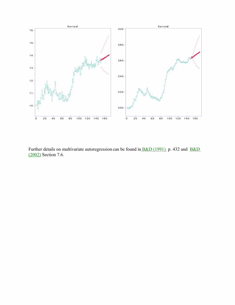
10.

11 .

12 .

13 .

14 .

15 .

16 .

0 20 40 60 80 100 120 140 160

S e r i e s 1

200.

220.

240.

260.

280.

300.

0 20 40 60 80 100 120 140 160

S e r i e s 2

Further details on multivariate autoregression can be found in B&D (1991) p. 432 and B&D (2002) Section 7.6.

PeriodogramSee also Smoothed Periodogram , Cumulative Periodogram, Model-standardized Cumulative Periodogram , Fisher’s Test , Model Spectral Density

Refs: B&D (1991) p.332. , B&D (2002) Section 4.2.

The periodogram of the data X1, . . . , Xn, is defined as

,||)( 21

1 jitn

t tj eXnI

where j = 2j/n, j=0,1, . . . , [n/2] , are the Fourier frequenciesin [0, and [n/2] is the integer part of n/2. The periodogramestimate of the spectral density at frequency j is

).(21)(ˆ

jj If

This function is plotted by selecting the Periodogram suboption ofthe Spectrum Menu.A large value of f̂ (j) suggests the presence of a sinusoidalcomponent in the data at frequency j. This hypothesis can betested as described in B&D (1991), Section 10.1. Alternatively onecan test for hidden periodicities (of unspecified frequency) by usingFisher’s test or by applying the Kolmogorov-Smirnov test to thecumulative periodogram.

Example: The periodogram estimate of the spectral density for theseries SUNSPOTS.TSM is obtained by opening the file in ITSM,clicking on the Spectrum Menu and then on the suboption Periodogram.

0.

500.

1000.

1500.

2000.

.0 .5 1.0 1.5 2.0 2.5 3.0

Cumulative PeriodogramSee also Periodogram , Model-standardized Cumulative Periodogram , Smoothed Periodogram, Fisher’s Test

Ref: B&D (1991) p.341.

Select Spectrum>Cumulative Spectrum>Periodogram to plot the standardizedcumulative periodogram of X1, …,Xn ,defined as the distribution function(assigning all of its mass to [0,

,,1,...,1,11

,1

,1,,0

)/2(qx

qiixx

YnxC i

where q = [(n - 1)/2],

q

k k

ki

ki

I

IY

1

1

)(

)(

and I(k) is the periodogram ordinate at the Fourier frequency k.If { X t } is Gaussian white noise, then Y i , i=1,…,q-1 are distributed asthe order statistics from a sample of q-1 independent uniform (0,1) randomvariables, and the standardized cumulative periodogram should beapproximately linear. The Kolmogorov-Smirnov test rejects the hypothesisof Gaussian white noise at level .05 if C(2x/n) exits from the boundaries

.1,)1(36.111)/2( 2/1 qxq

qxnxy

Example: The standardized periodogram of the series SUNSPOTS.TSM isobtained by opening the file in ITSM, and selecting Spectrum>CumulativeSpectrum>Periodogram. It is clear from the graph below that the Kolmogorov-Smirnov test rejects the hypothesis of Gaussian white noise at level .05.

.20

.40

.60

.80

1.00

.0 .5 1.0 1.5 2.0 2.5 3.0

.20

.40

.0 .5 1.0 1.5 2.0 2.5 3.0

To plot the Kolmogorav Smirnov bounds and carry out the test in a more general context (i.e. to test whether or not the data is compatible with any specifed ARMA spectral density f),use the options Spectrum>Cumulative Spectrum> Model-standardized .

Model-Standardized Cumulative PeriodogramSee also Periodogram, Cumulative Periodogram.

Ref: B&D (1991) p. 342.

The model-standardized cumulative periodogram is defined as the distribution function (with mass concentrated on [0,

,,1,...,1,11

,1

,1,,0

)/2(qx

qiixx

YnxC i

where q = [(n - 1)/2],

,)(/)(

)(/)(

1

1

kq

k k

kki

ki

fI

fIY

I(k) is the periodogram ordinate and f(k the model spectral density at the Fourier frequency k.If { Xt} is an ARMA process with the spectral density f , then Yi , i=1,…,q-1 are approximately distributed as the order statistics of a sample of q-1 independent uniform (0,1) random variables, and the model-standardized cumulative periodogram should be approximately linear. The Kolmogorov-Smirnov test rejects the hypothesis that the data is a sample from an ARMA process with the spectral density f at level .05 if C(2x/n) exits from the boundaries

.1,)1(36.111)/2( 2/1 qxq

qxnxy

These bounds are automatically plotted with the model-standardized cumulative periodogram, making it a trivial matter to test whether or not the data is compatible with the spectral density of the current model. ITSM also plots the level .01 bounds which are more widely spaced, with the constant 1.36 replaced by 1.63.

Example: Select the options File>Project>Open>Univariate, click OK and type SUNSPOTS to import the sunspot series with its default model of white noise. To see the model-standardized cumulative periodogram select Spectrum>Cumulative Spectrum>Model Standardized and you will see the following graph. Since the graph exits very convincingly from both the level.05 and level .01 Kolmogorov-Smirnov bounds, it is clear that white noise is an unsatisfactory model for SUNSPOTS.

.00

.20

.40

.60

.80

1.00

. 0 .5 1 . 0 1.5 2.0 2 . 5 3.0

CDF o f Per iodogram / Model Spect rum and K-S Bounds

Select Window>Tile to rearrange the windows and then try fitting a better model for SUNSPOTS. This can be done by choosing Model>Estimation>Preliminary, Yes (to subtract the mean before ARMA fitting) and then selecting Burg , Find AR model with min AICC and clicking OK. The model-standardized cumulative periodogram then changes automatically to reflect the new fitted model (an AR(8)) and we see from the graph below that the new model is an excellent fit insofaras the Kolmogorov-Smirnov bounds are concerned.

.00

.20

.40

.60

.80

1 . 00

.0 .5 1.0 1.5 2.0 2 . 5 3 . 0

CDF o f Per iodogram / Model Spectrum and K-S Bounds

Smoothed PeriodogramSee also Periodogram , Cumulative Periodogram , Model Spectral Density

Refs: B&D (1991) p.446. , B&D (2002) Section 4.2.

The spectral density of a stationary process can be estimated by smoothing the periodogram. The smoothed periodogramestimate of the spectral density at the Fourier frequency j is

),()(21)(ˆ

m

mk kjj IkWf

where the weights W(k) are non-negative, add to 1 and satisfyW(k) = W(-k). They are chosen by selecting the SmoothedPeriodogram suboption of the Spectrum Menu. You will then see the following dialog box:

The weights are generated by the successive application of nDaniell filters (filters with W(k) = 1/(2m+1), k= -m, . . . , m).The required value of n is first entered in the highlighted windowshown in the box above. Then using the mouse or tab key, enterthe order m of each of the filters 1, . . . , n. Once this has beendone you will see the weights {W(j)} corresponding to thesuccessive application of the n filters shown in the bottom window

of the dialog box. Pressing the Apply button will then generatethe corresponding smoothed periodogram spectral densityestimate.

Example: To apply the filter obtained by successive applicationof two Daniell filters with m=1 and m=3 we enter the value n=2,then Order of Filter 1 = 1 and Order of Filter 2 = 3. The weightsshown in the bottom window of the dialog box will then be

W0 = W1 = W2 =1/7, W3 = 2/21 and W4 = 1/21.Pressing the Apply button will cause the filter with these weights to be applied to the periodogram of the data and the resulting smoothed spectral density estimate will be plotted. Applying these weights tothe periodogram of the data in SUNSPOTS.TSM gives

0.

200.

400.

600.

800.

1000.

.0 .5 1.0 1.5 2.0 2.5 3.0

Preliminary EstimationSee also ACF/PACF , Maximum Likelihood Estimation , Constrained MLERefs: B&D (1991) Secs 8.2, 8.3, 8.4 , B&D (2002) Sec. 5.1.

The option Estimation in the Model Menu has two suboptions, Preliminaryand Maximum Likelihood. The Preliminary methods are fast (but somewhatrough) algorithms. They are useful for suggesting the most promising modelsfor the data, but they should be followed by the more refined maximumlikelihood method. Once you have fitted a preliminary model, the likelihoodmaximization algorithm will use it as the starting point in the search for theparameter values which maximize the (Gaussian) likelihood.

On selection of the Preliminary Estimation option, you will see the followingdialogue box:

To fit an AR(p) model, enter the value of p in the AR order window and thenselect either the Yule-Walker or Burg algorithm. (The default, as shown in thedialogue box above, is Yule-Walker. However the Burg estimates frequentlygive larger Gaussian likelihoods.)

To fit an ARMA(p,q) model with q>0, the required values of p and q must beentered in the AR order and MA order windows respectively. Once these havebeen entered you will have a choice between the Hannan-Rissanen andInnovations algorithms. The latter frequently gives larger likelihoods whenp=0 while Hannan-Rissanen has a greater tendency to give causal models asrequired by the program when p>0. If the chosen preliminary estimationalgorithm gives a non-causal model then all coefficients will be set to .001 togenerate a causal model with the specified values of p and q. The parameterNumber of ACVF's appearing in the bottom right of the dialogue box is aparameter of the Innovations algorithm (B&D (1991), Secs 8.3-8.4 or B&D(1996), p.149) which will usually be set to the default value by entering zero.

Our ultimate objective is to find a model with as small an AICC value aspossible, where AICC (see B&D (1991), Sec. 9.3 or B&D (1996), Sec. 5.5.2)is defined as

p=0 while Hannan-Rissanen has a greater tendency to give causal models asrequired by the program when p>0. If the chosen preliminary estimationalgorithm gives a non-causal model then all coefficients will be set to .001 togenerate a causal model with the specified values of p and q. The parameterNumber of ACVF's appearing in the bottom right of the dialogue box is aparameter of the Innovations algorithm (B&D (1991), Secs 8.3-8.4 or B&D(1996), p.149) which will usually be set to the default value by entering zero.

Our ultimate objective is to find a model with as small an AICC value aspossible, where AICC (see B&D (1991), Sec. 9.3 or B&D (1996), Sec. 5.5.2)is defined as

AICC = -2ln L + 2(p + q + 1)n/(n - p - q - 2)where L is the Gaussian likelihood (see B&D (1991), eqn (8.7.4) or B&D(1996), eqn (5.2.9). Smallness of the AICC value computed under PreliminaryEstimation is indicative of a good model but should only be used as a roughguide. Final decisions between models should be based on maximum likelihoodestimation, since for fixed p and q the values of the parameters which minimizethe AICC statistic are the maximum likelihood estimates, not the preliminaryestimates. It is possible to minimize the AICC of preliminary pure autoregressivemodels (over the range p=0 to 26) by selecting either Burg or Yule-Walker andchecking the Find AR with min AICC box.

Example: The following output from ITSM was obtained by opening the data fileSUNSPOTS.TSM, selecting Model-Estimation-Preliminary, subtracting the meanand clicking on Burg, Min AICC, then OK. The ratios of coefficients to 1.96 timesstandard errors suggests the possibility of fitting a subset autoregression with 5 andpossibly equal to zero. This can be done under maximum likelihood estimation.

=================================ITSM2000:(Preliminary estimates)=================================Method: Burg (Minimum AICC)

ARMA Model: X(t) = 1.512 X(t-1) - 1.095 X(t-2) + .4822 X(t-3) - .1963 X(t-4)

+ .01121 X(t-5) + .1013 X(t-6) - .2054 X(t-7) + .2502 X(t-8)+ Z(t)

WN Variance = 189.609808

AR Coefficients1.511890 -1.095235 .482203 -.196292.011207 .101345 -.205432 .250184

Ratio of AR coeff. to 1.96 * (standard error)8.663315 -3.734065 1.501416 -.611676.034922 .315554 -.700395 1.433584

(Residual SS)/N = 189.610

WN variance estimate (Burg): 176.429

-2Log(Like) = 811.877882AICC = 831.877882

Regression with ARMA or ARFIMA ErrorsSee also Model Specification, ARMA Forecasts .Refs: B&D (1991) Sec.13.2, B&D (2002) Section 6.6.

Classical regression analysis is concerned with fitting a model of the form,,,,1,11 ntWxxY tktktt

to observations of Y at times t=1,…,n, expressing them in terms of k explanatory variables x and noise terms (or residuals) W , where the noise terms at times t=1,…,n, are independent and identically distributed. Regression with ARMA errors deals with the same problem except that W is assumed instead to be an ARMA process whose parameters are to be estimated. In matrix notation, the model is

Y = X W,Where

)',,( 1 nYYY ,kjnttjxX ,..,1;,..,1][ ,

)',,( 1 k ,)',,( 1 nWWW

and).,0(~}{,)()( 2 WNZZBWB ttt

Particular cases which arise frequently in applications areLinear Trend. :

txx tt 21 ,1 .Harmonic Regression.

).sin(),cos(,1 321 txtxx ttt

Arbitrary Regressors. Any prespecified functions x1,…,xm , whose values for t=1,…,n, are stored as m columns in an ASCII file (with .TSM suffix) can also be used as regressors. See also Intervention AnalysisARFIMA Errors. Regression with Long Memory Errors follows the same steps set out below with the obvious modification of the MLE step.

We illustrate below by fitting a linear trend with ARMA noise to LAKE.TSM and a step-function regressor to the series CDID.TSM.

Example 1.To fit a linear trend function with ARMA errors to LAKE.TSM, first import the data into ITSM by selecting File>Project>Open>Univariate then LAKE.TSM. Then click Regression>Specify and complete the regression dialog box as shown.

Then click OK and press the GLS button. Since the default model in ITSM iswhite noise, the generalized least squares estimates of the coefficients in

98,,1,21 ttYt will be the same as the ordinary least squares estimates at this first iteration.These are shown in the Regression Estimates window.

Press the yellow Plot Sample ACF/PACF button to see the ACF/PACF of theresiduals, which appear to have the PACF of an AR(2) model. SelectingModel>Estimation>Preliminary and choosing Burg estimation with the minimumAICC option confirms this model. Then choose Model>Estimation>MaxLikelihood to obtain the maximum likelihood AR(2) model for the residuals.

GLS STEP. Press the GLS button again and the generalized least squaresestimates corresponding to the previously found AR(2) model for the residualswill be shown in the Regression Estimates Window.MLE STEP. Again choose Model>Estimation>Max Likelihood to obtain theupdated AR(2) model for the new residuals.

Alternate the GLS and MLE steps until the coefficient estimates stabilize. Aftertwo iterations we find the model,

Method: Generalized Least SquaresY(t) = M(t) + X(t)

Trend Function:M(t) = 10.091444 t^0 - .021576732 t^1

ARMA Model:X(t) = 1.008 X(t-1) - .2947 X(t-2) + Z(t)

WN Variance = .457128

Coeff Value Std Error

Alternate the GLS and MLE steps until the coefficient estimates stabilize. Aftertwo iterations we find the model,


Trend Function:M(t) = 10.091444 t^0 - .021576732 t^1

ARMA Model:X(t) = 1.008 X(t-1) - .2947 X(t-2) + Z(t)

WN Variance = .457128

Coeff Value Std Error0 10.09144424 .462267611 -.02157673 .00804851

X(t) = 1.005 X(t-1) - .2913 X(t-2) + Z(t)WN Variance = .456614

Coeff Value Std Error 0 10.09139847 .463236301 -.02156431 .00806457

WARNING. If you are using a fractionally integrated model for the residuals with thousands of observations, the iteration step may take minutes. If the Regression Estimates window is closed, the iteration step will update the model for the residuals without updating the regression coefficients. This is a much faster operation.

Example 2.To estimate b and find a suitable ARMA model for {W(t)} in the regression model,

X(t)=bg(t)+W(t),where {X(t)} is stored in the file SBLD.TSM (see Data sets , B&D (2002) Example 6.6.3) and {g(t)} is stored in SBLDIN.TSM, proceed as in the preceding example, but in the Regression Trend Function dialog box shown above uncheck the Polynomial Regression and Include Intercept options and check the option Include Auxiliary Variables. When you have done this, click on Browse, type SBLDIN and click on open. Specify 1 for the number of columns (since there is only one regressor stored in SBLDIN.TSM) and click OK. Then click OKin the Regression Trend Function dialog box and you are ready to begin the regression.

Press the blue GLS button and you will see the ordinary least squares regression model,X(t)=-346.2g(t)+W(t),

displayed in the Regression Estimates window together with the assumed noise model (white noise in this case). .Leaving this window open, press the yellow Plot Sample ACF/PACF button to see the ACF/PACF of the residuals. The sample ACF and PACF suggests an MA(13) or AR(13) model for {W(t)}. Fitting AR and MA models of orders up to 13 (with no mean correction) using the option Model>Estimation>Autofit gives an MA(12) model as the minimum AICC fit for the residuals. Once this model has been fitted, the model in the Regression Estimates window is automatically updated to

X(t)=-328.45g(t)+W(t),with the fitted MA(12) model for the residuals also displayed.

ITERATION. Pressing the MLE button again will cause both the regression estimates and the ARMA model for the residuals to be updated.

Repeat the iteration step until the values in the Regression Estimate window stabilize. This will take just a few iterations and give the results:

========================================ITSM::(Regression estimates)========================================


Trend Function: M(t) = - .32844534E+03 x(1)

ARMA Model: X(t) = Z(t) + .2189 Z(t-1) + .09762 Z(t-2) + .03093 Z(t-3)+ .06447 Z(t-4) + .06878 Z(t-5) + .1109 Z(t-6) + .08120 Z(t-7)+ .05650 Z(t-8) + .09192 Z(t-9) - .02828 Z(t-10) + .1826 Z(t-11)- .6267 Z(t-12)

WN Variance = .125805E+05

Coeff Value Std Error 1 -.32844534E+03 49.41040178

Note. This model is a little different from the one obtained by Intervention Analysis. The intervention model is fitted by least squares. The difference between the estimated regression coefficients is less than the standard error given above.

To see the fitted regression with the data, click on Regression>Show fit and you will see the following graph:

-600.

-400.

-200.

0 .

200 .

400 .

0 20 40 60 8 0 1 00

Further details on regression with ARMA errors can be found in B&D (2002) Section 6.6.

Residual PlotsSee also ACF-PACF , Residual Tests , Preliminary Estimation . Refs: B&D (1991) Sec.9.4, B&D (1996) Sec.5.3.

The option Residual Analysis in the Statistics Menu provides four suboptions,Plot, Histogram, ACF/PACF and Tests of Randomness. Each of these enablesyou to examine properties of the residuals of the data from the current modeland hence to check whether or not the model provides a good representationof the data.

The residuals are defined to be the rescaled one-step prediction errors,,/)ˆ(ˆ

1 tttt rXXW

where tX̂ is the best linear mean-square predictor of Xt based on the data up totime t - 1, is the white noise variance of the fitted model and

221 /)ˆ( ttt XXEr .

If the data were truly generated by the current ARMA(p, q) model with whitenoise sequence {Zt }, then for large samples the properties of the residuals shouldreflect those of {Zt } (see B&D (1991), Sec.9.4, or B&D (1996), Sec.5.3). Tocheck the appropriateness of the model we can therefore examine the residualseries and check that it resembles a white noise sequence.

The suboption Plot generates a time-series graph of the data which should bechecked for signs of trend, cycles, non-constant variance and any other apparentdeviations from white-noise behaviour.

The suboption Histogram generates a histogram of the residuals which shouldhave mean close to zero. If the fitted model is appropriate and the series isGaussian, this will be reflected in the shape of the histogram of the residualswhich should then resemble a normal density with mean zero and variance equalto the white noise variance of the fitted model.

The suboption ACF/PACF plots the sample ACF and PACF of the residualSeries, both of which should lie between the bounds n/96.1 for roughly95% of the lags greater than 0. If substantially more than 5% lie outside theselimits, or if there are a few very large values, then we should look for a better-fitting model. (More precise bounds, due to Box and Pierce, can be found inB&D (1991), Sec.9.4.)

Example: Read the data SUNSPOTS.TSM into ITSM, subtract the mean andthen select the options Model-Estimation-Preliminary to fit the minimum AICCBurg AR model to the mean-corrected series. This will be an AR(8). Thenselect Statistics-Residual Analysis-Plot and Statistics-Residual Analysis-ACF/PACF and you will see the first two graphs below. Neither graph showsany apparent deviation from white noise behaviour, however examination of thehistogram of the residuals suggests that the assumption of Gaussian white noisein this model may not be appropriate.

40.

Example: Read the data SUNSPOTS.TSM into ITSM, subtract the mean andthen select the options Model-Estimation-Preliminary to fit the minimum AICCBurg AR model to the mean-corrected series. This will be an AR(8). Thenselect Statistics-Residual Analysis-Plot and Statistics-Residual Analysis-ACF/PACF and you will see the first two graphs below. Neither graph showsany apparent deviation from white noise behaviour, however examination of thehistogram of the residuals suggests that the assumption of Gaussian white noisein this model may not be appropriate.

-40.

-30.

-20.

-10.

0.

10.

20.

30.

40.

0 20 40 60 80 100

-1.00

-.80

-.60

-.40

-.20

.00

.20

.40

.60

.80

1.00

0 5 10 15 20 25 30 35 40

Residual ACF

-1.00

-.80

-.60

-.40

-.20

.00

.20

.40

.60

.80

1.00

0 5 10 15 20 25 30 35 40

Residual PACF

2.

4.

6.

8.

10.

12.

14.

16.

18.

20.

-30 -20 -10 0 10 20 30 40

Residual TestsSee also Residual Plots , Preliminary Estimation . Refs: B&D (1991) Sec.9.4 , B&D (1996) Sec.5.3.

If the current ARMA model is appropriate for the current data set, then theresiduals (see Residual Plots) should have properties consistent with those ofa white noise sequence. This can be checked by looking at residual plots andby carrying out the following randomness tests , described in detail in theabove references to B&D.

1. Ljung-Box portmanteau test2. McLeod-Li portmanteau test3. Turning point test4. Difference-sign test5. Rank test6. Minimum-AICC AR order

The statistics, used in 1, 3, 4 and 5 have known large-sample distributionsunder the hypothesis of independent and identically distributed random data.These distributions are specified in the output of ITSM together with theobserved value of each sample statistic. The same is true for 2, except thatthe additional hypothesis of normality is required. The p-value for each testis also shown. This is the probability of obtaining a value of the test statisticas extreme as, or more extreme than, the value observed, under the assumptionthat the null hypothesis of iid random data is true. A p-value less than .05 (forexample) indicates rejection of the null hypothesis at significance level .05.

In test 6 the, Yule-Walker algorithm (see Preliminary Estimation) is applied tothe residuals and the AR model with minimum AICC (for orders p up to 26) isdetermined. If the residuals are white noise, this value should be 0.

Example: Read the data AIRPASS.TSM into ITSM, and use the Transformoption of ITSM to take logarithms (Box Cox transformation with parameter zero),difference at lags 12 and 1 and finally to subtract the mean of the transformedseries. Then select the options Model>Estimation>Preliminary to fit the minimumAICC Burg AR model to the resulting series. This turns out to be an AR(12)model. Then select Statistics>Residual Analysis>Tests of Randomness and youwill be asked to select the parameter h for the two portmanteau tests. Accepting thedefault value of 32, you will see the test results below.

============================================ITSM2000:(Tests of randomness on residuals)============================================

Ljung - Box statistic = 29.993 Chi-Square ( 20 ), p-value = .06996

McLeod - Li statistic = 43.346 Chi-Square ( 32 ), p-value = .08696

# Turning points = 89.000~AN(86.000,sd = 4.7924), p-value = .53132

# Diff sign points = 68.000~AN(65.000,sd = 3.3166), p-value = .36571

# Rank points = .41790E+04~AN(.42575E+04,sd = .25130E+03), p-value = .75476

ITSM2000:(Tests of randomness on residuals)============================================

Ljung - Box statistic = 29.993 Chi-Square ( 20 ), p-value = .06996

McLeod - Li statistic = 43.346 Chi-Square ( 32 ), p-value = .08696

# Turning points = 89.000~AN(86.000,sd = 4.7924), p-value = .53132

# Diff sign points = 68.000~AN(65.000,sd = 3.3166), p-value = .36571

# Rank points = .41790E+04~AN(.42575E+04,sd = .25130E+03), p-value = .75476

Order of Min AICC YW Model for Residuals = 0

None of the tests rejects the hypothesis of iid residuals at level .05 and theminimum-AICC Yule Walker AR model for the residuals is of order zero.These observations, and inspection of the sample ACF of the residuals, allsupport the adequacy of the fitted model.

SimulationSee also Classical Decomposition , Model Specification . Refs: B&D (1991) p. 271.

ITSM can be used to generate realizations of a random time series defined bythe current ARMA model. To generate such a realization, select the Model Menu,then the option Simulate and you will see a dialogue box like the following:

If you have applied transformations to the original series to arrive at the currentdata set, then you will have the opportunity, by checking the appropriate choicesin the dialogue box, to apply the inverse transformations to the simulated ARMAseries in order to generate a simulated version of the original series. The defaultwhite-noise distribution used for simulation is normal, however if you press theChange noise distribution button, you will be given the choice of distributionsshown in the following dialogue box.

Example: Read the data AIRPASS.TSM into ITSM and, with the aid of theTransform Menu, apply the Box-Cox transformation with parameter 0, and makea Classical Decomposition of the resulting series into a seasonal component withperiod 12 and a linear trend. The mean of the residuals is so close to zero that there is no need to subtract the mean.

To fit a simple model to the transformed data select Model>Estimation>Preliminaryand determine the minimum AICC Burg AR model. This is an AR(2).

To use this model for the transformed data to simulate a realization of the originaldata, select the Model Menu followed by the option Simulate. You should then seethe top dialogue box shown above. The default number of observations to be simulatedis the same as the number of original data. The seed is an integer of 10 or fewerdigits which initializes the random number generator. If at some time you wish togenerate an exact replica of the simulated realization, it can be done by ensuring thatthe seed is set to the same value, which in this case is 102452. To generate anotherindependent realization, change the seed number while keeping all other parametersthe same. The white noise variance is that of the fitted model (1.214 x 0.001) and themean to be added to the simulated ARMA is zero since we did not subtract the mean from the transformed data. The two check marks indicate that we wish to add theestimated trend and seasonal components to the simulated ARMA and apply theinverse Box-Cox transformation to the resulting series. In this way we should obtaina simulated version of the original series. Eliminating these check marks by clickingon them would lead to a realization of the AR(2) process fitted to the residual series.The simulated realization of the original series (using normally distributed noise) is shown below.

100.

200.

300.

400.

500.

600.

0 20 40 60 80 100 120 140

Spectral(FFT) Smoothing

See also Moving Average Smoothing, Exponential smoothing,

Ref: B&D (2002) Section 1.5.

Spectral smoothing is accomplished by removing the high frequency components from the series. This involves three steps, first the FFT of the series is calculated second the Fourier coefficients above a chosen cutoff frequency are set to zero, lastly, the inverse FFT is taken of the modified spectrum resulting in the smoothed sequence.

After selecting the suboption FFT Smooth from the Smooth menu, a dialog box will open requesting you to enter a smoothing parameter f betwen 0 and 1. The smaller the value of f the more the series is smoothed with maximum smoothing ocurring when f=0.

Once the parameter f has been entered, the program will graph the smoothed time series with the original data and will display the root of the average squared deviation of the smoothed values from the original observations defined by


nj

11

2

Further details on spectral smoothing may be found in B&D (2002) p.19.

Subsequence

The option Subsequence of the Transform Menu allows us to analyze asegment of the time series obtained by eliminating specified numbers ofdata from the beginning and/or end of the series.

Example: Suppose we open the project SUNSPOTS.TSM which consists of100 observations X1, … ,X100, but wish to analyze only the second half of theseries. This is achieved by selecting the Subsequence option of the TransformMenu, at which point you will see the following Subsequence Dialogue Box.

To select the last half of the series, simply enter 51 in the window labelled Minand leave the default entry 100 as it is in the Max window. Then press the OKbutton and you will see that the data window labelled SUNSPOTS.TSM nowcontains a graph of only the 50 last observations of the original series. If you hadalready opened the ACF/PACF window for SUNSPOTS.TSM, this would alsochange to reflect the change in the data set SUNSPOTS.TSM. If you wish torecover the original series select the Undo option of the Transform Menu.

Transfer Function ModellingSee also Intervention Analysis.

Outline: Given observations of an ``input’’ series {U(t)} and ``output’’ series {V(t)}, The steps in setting up a transfer function model relating V(t) to U(t) and U(s), s<t, begin with differencing and mean correction to generate transformed input and output series {X(t)}and {Y(t)} respectively, which can be modelled as zero-mean stationaryprocesses. The objective then is to fit a transfer function model of the form,

,)()()()(0

jtNjtXjtY

where {N(t)} is an ARMA process uncorrelated with {X(t)},),,0(~)}({),()()()( 2

WNN WNtWtWBtNB the transfer function, T(B), is assumed to have the form,

,1(

)()(1

)10

0 pp

qq

d

jj

BvBvBwBwwB

BjBT

and the input process {X(t)} is assumed to be an ARMA process,).,0(~)}({),()()()( 2

ZXX WNtZtZBtXB The parameters in the last three equations are all to be estimated from the givenobservations of (X(t),Y(t)). Residual correlations and cross-correlations can be computed for model checking. The AIC value of the fitted model is computedfor model comparisons, and forecasts of Y(t) (and of the original output series V(t)) are computed from the fitted model. The steps are illustrated in the following example.

Example. Select the options File>Project>Open then click Multivariate, OK, and select the file LS2.TSM. This file contains two columns,the first being a leading indicator and the second a sales figure. In the following dialog box you can therefore accept the default value 2 for the number of columns and click OK. The following graphs of the input and output series will then appear.

9.50

10.00

10.50

11.00

11.50

12.00

12.50

13.00

13.50

14.00

0 20 40 60 80 100 120 140

Ser ies 1

200.

210.

220.

230.

240.

250.

260.

0 20 40 60 80 100 120 140

Ser ies 2

Select the options Transform>Difference and difference at lag 1, then Transform>Subtract Mean to produce two stationary-looking series {X(t)} and {Y(t)}.

Click on the Export button at the top right of the ITSM window and export thetransformed time series to the Clipboard. Open Microsoft Excel and paste the contents of the clipboard which will appear as two adjacent columns in Excel.Copy the first column, {X(t)}, and paste it into a Notepad file, then save it as DLEAD.TSM in the ITSM6 directory. Repeat for the second column, giving it the name DSALES.TSM. Return to ITSM, where the screen should still show the graphs of {X(t)} and {Y(t)}. Without closing the original bivariate project,proceed through the following steps.Modelling {X(t)}: Select File>Open>Project>Univariate and select DLEAD.TSM.The univariate toolbar will then reappear at the top of the ITSM window. Clicking on the Plot Sample ACF/PACF button and inspecting the sample ACF suggests an MA(1) model for {X(t)}. The maximum likelihood MA(1) model is found to be (see Preliminary Estimation and Maximum Likelihood Estimation,)

).07794,.0(~)}({),1(4744.)()( WNtZtZtZtX (The mean is not subtracted from {X(t)} for this calculation.)Export X-Residuals: Press the Export Button and in the dialog box select Residuals and Clipboard.and then click OK. Paste these residuals into a spreadsheet column in Excel. Also paste them into a notepad file and save as the file XRES.TSM.Import {Y(t)}: With the DLEAD.TSM window highlighted, select File>Import File and type DSALES.TSM. without changing the MA(1) model fitted above,Export Y-Residuals: Press the Export Button, in the dialog box select Residuals and Clipboard.and then click OK. Paste these residuals into the spreadsheet column immediately to the right of the column containing the corresponding X-residuals.Import Bivariate X-Y-Residuals: Mark the 149 by 2 array in the Excel spreadsheetcontaining the X- and Y-residuals, click Copy, and then return to ITSM. Now, makingsure that the LS2.TSM window is highlighted, select File>Import Clipboard andthe graphs of the bivariate series of X- and Y-residuals will appear in the window labelled LS2.TSM.

Preliminary Transfer Coefficients: Press the Plot Sample Cross Correlationsbutton and you will see the array of cross-correlation graphs shown below.

-1.00

-.80

-.60

-.40

-.20

.00

.20

.40

.60

.80

1.00

0 2 4 6 8 10 12 14 16 18 20

Series 1

-1.00

-.80

-.60

-.40

-.20

.00

.20

.40

.60

.80

1.00

0 2 4 6 8 10 12 14 16 18 20

Series 1 x Series 2

-1.00

-.80

-.60

-.40

-.20

.00

.20

.40

.60

.80

1.00

0 2 4 6 8 10 12 14 16 18 20

Series 2 x Series 1

-1.00

-.80

-.60

-.40

-.20

.00

.20

.40

.60

.80

1.00

0 2 4 6 8 10 12 14 16 18 20

Series 2

The upper right and lower left graphs show that the Y-residual at time t+h is significantly correlated with the X-residual at time t for h=3,…,9, but not otherwise.This suggests a transfer function model (see above) with j) non-zero for j=3,…,9,and zero otherwise. The estimated values of j) are (see B&D (2002) Section 10.1

12 /)()( jj where (j) is the correlation between the Y-residual at time t+j and the X-residual at time tRight-clicking on the graphs of the cross correlations and selecting Info gives

,1846.)9(,,4718.)4(,6768.)3( .and right clicking on the graphs of the residuals and selecting Info gives

0055.2,2792.0 21 .These give preliminary coefficient estimates

.326.1)9(,,389.3)4(,861.4.)3( (The arithmetic can be carried out in Excel by clicking the Export button, selecting Sample ACF and then pasting the exported cross correlations into a spreadsheet..)The next step is to use a more efficient estimation procedure with these 7 coefficientsas preliminary estimates. However the approximately geometric rate of decay ofthe preliminary estimates suggests fitting instead the two-parameter transferfunction

,1

)(1

30

BvBw

BT

with the preliminary estimates,.7.0,86.4 10 vw

Least Squares Estimation: We are now ready for more efficient estimation of the parameters in our preliminary model. Close ITSM, reopen it and reopen the original project LS2.TSM consisting of the Leading indicator and Sales series.

Difference at lag 1 and subtract the mean as above. Select Transfer>Specify Modeland complete the first two pages of the dialog box as follows, clicking OK when they are completed.

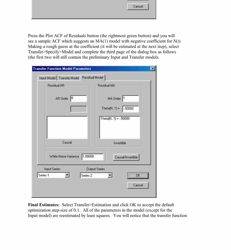
Press the Plot ACF of Residuals button (the rightmost green button) and you willsee a sample ACF which suggests an MA(1) model with negative coefficient for N(t).Making a rough guess at the coefficient (it will be estimated at the next step), select Transfer>Specify>Model and complete the third page of the dialog box as follows(the first two will still contain the preliminary Input and Transfer models.

Final Estimates: Select Transfer>Estimation and click OK to accept the defaultoptimization step-size of 0.1. All of the parameters in the model (except for theInput model) are reestimated by least squares. You will notice that the transfer function

residuals (which are estimates of the noise W(t) in the model for N(t)) now appear, asthey should, to be uncorrelated. To refine the fit, again select Transfer>Estimation, select step-size 0.01 and click OK. You will notice an improvement in the fit, withthe AICC value now down to 29.932. Refining the fit several more times gives the model,.

========================================ITSM2000:(Transfer Function Model Estimates)========================================

X(t,2) = T(B) X(t,1) + N(t)

B^3(4.717)T(B) = -----------------

(1 -.7248 B^1)

X(t,1) = Z(t) - .4740 Z(t-1){Z(t)} is WN(0,.077900)

N(t) = W(t) - .5825 W(t-1){W(t)} is WN(0,.048643)

AICC = 27.664882

Accuracy Parameter .000010

Alternative models (e.g. the moving average transfer-funcion model with seven coefficients introduced above) can also be explored in the hope of finding another model with smaller AICC. We shall not do that here, but instead demonstrate thecorrelation checks for goodness of fit of the model just determined.Residual Checking: Press the Export button, select Residuals and Clipboard andpress OK. Open Notepad, paste in the Noise residuals and save in the ITSM2000 directoryas NRES.TSM. Now we can check the correlations and cross correlations of theInput and Noise residuals as follows. Select File>Open>Project>Multivariate with one column and open the Input residual file XRES.TSM created earlier. Then select File>Open>Project>Univariate NRES.TSM. To create a bivariate projectpress the Project Editor button (the leftmost button), click on the plus signs beside each of the two projects XRES.TSM and NRES.TSM to display the files in eachproject.. Next click on the file Series in the project NRES, drag the file to theproject XRES and click. Confirm the transfer of data in the dialog box which then appears and the project XRES will now contain both the input and noise residuals. You can rename the files in XRES by double-clicking on their names andtyping in new names (e.g. XRES and NRES). Click OK in the Project Editor window. Highlight the window XRES.TSM and press the Plot Sample ACF/PACF button and you will see the following graph. It shows clearly that

there are no significant correlations between the input and noise residuals, thusconfirming our confidence in the fitted transfer-function model.

-1.00

-.80

-.60

-.40

-.20

.00

.20

.40

.60

.80

1.00

0 2 4 6 8 10 12 14 16 18 20

Series 1

-1.00

-.80

-.60

-.40

-.20

.00

.20

.40

.60

.80

1.00

0 2 4 6 8 10 12 14 16 18 20

Series 1 x Series 2

-1.00

-.80

-.60

-.40

-.20

.00

.20

.40

.60

.80

1.00

0 2 4 6 8 10 12 14 16 18 20

Series 2 x Series 1

-1.00

-.80

-.60

-.40

-.20

.00

.20

.40

.60

.80

1.00

0 2 4 6 8 10 12 14 16 18 20

Series 2

Forecasting: The output series can be forecast up to twenty steps ahead using the fitted transfer function model. To do this for the current example, select Forecasting>Transfer-function, then in the dialog box enter 20 for the number of predictors, check the box to plot 95% prediction bounds and click OK. You will then see the following graph of predicted future sales and corresponding bounds.

Further details on transfer-function models can be found in B&D (1991) p. 506or B&D (2002) p.323.

200.

220.

240.

260.

280.

0 20 40 60 80 100 120 140 160

S e r i e s 2

TSM FilesSee also GETTING STARTED, Data sets.

All ITSM projects are stored in files with the suffix .TSM. The simplest of these contain data only. A multivariate time series with m components should be stored in an ASCII file with a name such as MYFILE.TSM, and with the data in m columns, one for each component.

Data and graphs can be saved at any time as described in GETTING STARTED.

You can also save the entire project by using the Save Project As button, fourth from the left on the toolbar at the top of the ITSM2000 screen. The resulting file will contain the current data, the transformations which have been applied to the original data, as well as the current model and the residuals, so that further analysis or comparisons with other models can be made at a later date. If you have renamed one or more series in a project, they will be saved with the new names.

Warning !.TSM files are all in ASCII format and can be edited with any text editor such as Notepad. Editing a project file of the type described in the previous paragraph must however be done with great care so as not to introduce inconsistencies into the saved project.

Examples. To see an example of a file containing data only, use notepad to open the file LS2.TSM. To see an example of a more elaborate TSM file saved as a project from ITSM, open the file STOCK7.TSM.

ITSM2000 - Home | York University · AR-Model>Estimation>Burg or AR-Model>Estimation>Yule-Walker....

Documents

Transcript of ITSM2000 - Home | York University · AR-Model>Estimation>Burg or AR-Model>Estimation>Yule-Walker....