It’s About Time

Mark Otto

U. S. Fish and Wildlife Service

Introduction

• Analyzing data through time

• ARIMA models

• Regression and time series

• Trends and differences

• Interventions

• Structural models

• Time series on survey data

Monitoring

• Background data to assess environmental change

• Past data at the same site and/or control data at “similar” sites

Monitoring

• Background data to assess environmental change

• Past data at the same site and/or control data at “similar” sites

• Measure the right variables in the right places before the change

Time Series Data

• Consistently observed

• Usually equally spaces in time– Annually– Monthly– Daily …

• No missing observations

Time Series Data-2

• Most population and habitat data taken over time

Time Series Data-2

• Most population and habitat data taken over time

• Expect patterns and relationships

• Data not independent

Time Series Data-2

• Most population and habitat data taken over time

• Expect patterns and relationships• Data not independent• OLS, ANOVA, GLIM• One time series not equal to one observation• Non-parametric

Time Series Analysis

• Data y, n observations

• n2 covariance parameters

Time Series Analysis

• Data y, n observations

• n2 covariance parameters

• Covariance of observation i steps same

• Less than n covariance parameters

Time Series Analysis-2

• Relation of two variables: correlation

• Relation with of variable with itself i steps ago: autocorrelation

• Use autocorrelations to decide on model

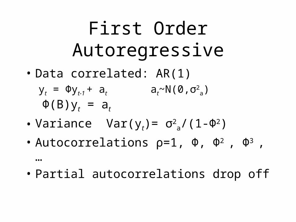
First Order Autoregressive

• Data correlated: AR(1)yt = Φyt-1 + at at~N(0,σ2

a)

Φ(B)yt = at

• Variance Var(yt)= σ2a/(1-Φ2)

• Autocorrelations ρ=1, Φ, Φ2 , Φ3 , …

• Partial autocorrelations drop off

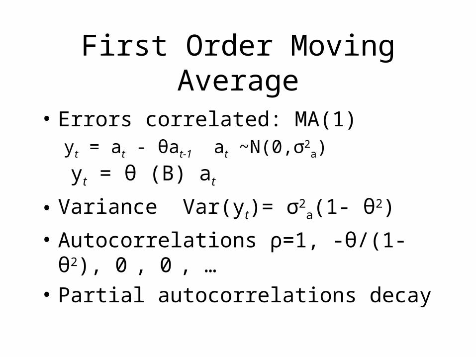
First Order Moving Average

• Errors correlated: MA(1)yt = at - θat-1 at ~N(0,σ2

a)

yt = θ (B) at

• Variance Var(yt)= σ2a(1- θ2)

• Autocorrelations ρ=1, -θ/(1- θ2), 0 , 0 , …

• Partial autocorrelations decay

First Order Moving Average-2

• Used in the stock market

• Made from running averages: early smoothing

ARIMA Models

• Data show how to model the series– AR: ACFs decay exponentially, PAFCs drop

off– MA: ACFs drop off, PACFs decay

exponentially

• Estimate model

• Check that the residuals are white noise

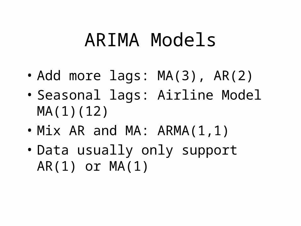
ARIMA Models

• Add more lags: MA(3), AR(2)

• Seasonal lags: Airline Model MA(1)(12)

• Mix AR and MA: ARMA(1,1)

• Data usually only support AR(1) or MA(1)

Stationarity

• Mean and variance constant

Stationarity

• Mean and variance constant

• Transform to stationarity– Box-Cox transform– Regression mean– Difference

Stationarity-2

• Count data follows a Poisson

• Log is canonical transformationlog(yt)-log(yt-1)=c+at

• Trend in the relative growthmean((yt- yt-1)/ yt-1 )=ec-1

Regression and Time Series

• Regression describes the mean

• ARIMA model describes the variance

• Regression parameters unbiased

• Regression standard errors are

• Most variance explained by regression

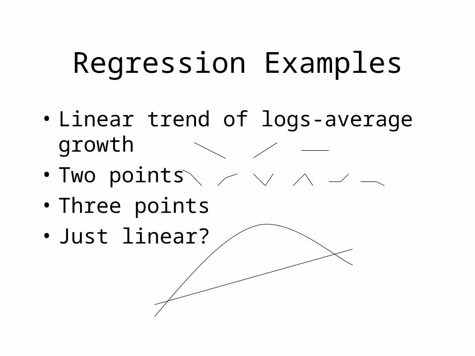
Regression Examples

• Linear trend of logs-average growth

• Two points

• Three points

• Just linear?

Regression Examples

• Relate to environment– Linear regression– Nonlinear relation

• Adds explanatory power to model

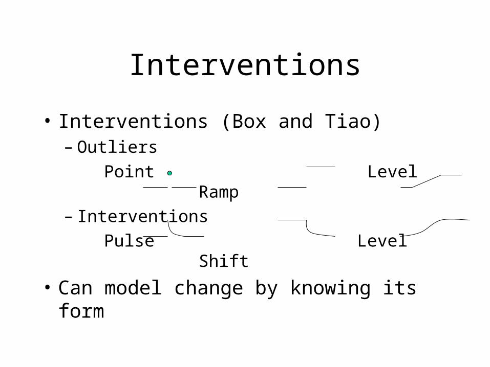
Interventions

• Interventions (Box and Tiao)– Outliers

Point Level Ramp– Interventions

Pulse Level Shift

• Can model change by knowing its form

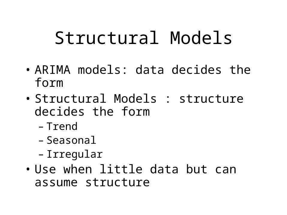
Structural Models

• ARIMA models: data decides the form• Structural Models : structure decides the

form– Trend– Seasonal– Irregular

• Use when little data but can assume structure

Time Series and Surveys

• Time points not just one observation Yt=Yt+et et~N(0,vt)

• Time points have mean and variance

• Could model the survey sample variance with a generalize variance function (GVF) and ARMA model

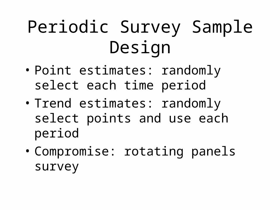
Periodic Survey Sample Design

• Point estimates: randomly select each time period

• Trend estimates: randomly select points and use each period

• Compromise: rotating panels survey

Time Series and Surveys-2

• Statistics on statistics (Link, Bell and Hillmer, Binder) Φ(B)Δ(B)(Yt-x'tβ)=ut ut~N(0,σ2

u)

• Hierarchial model that separates the survey error from the process

• Estimates are a compromise between the survey estimates and the model

What’s the difference

• Estimate changes Δ(B)Yt= Yt- Yt-1=ut ut~N(0,σ2

u)

• Nonstationary, mean and or variance vary

• Cannot use linear prediction

• Use E(Yt |yt) = yt- E(et | Δ(B) yt)

• Differencing tests not powerful

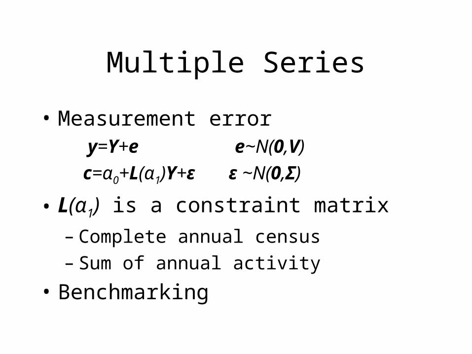
Multiple Series

• Measurement error y=Y+e e~N(0,V)

c=α0+L(α1)Y+ε ε ~N(0,Σ)

• L(α1) is a constraint matrix

– Complete annual census– Sum of annual activity

• Benchmarking

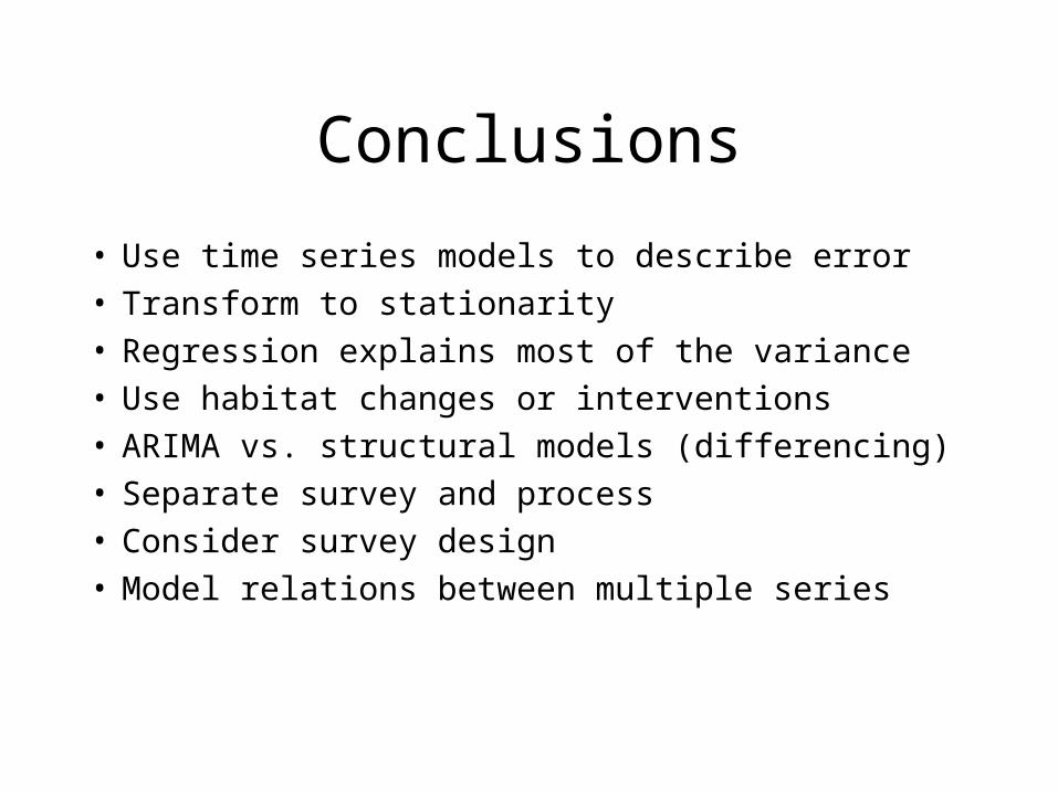
Conclusions

• Use time series models to describe error• Transform to stationarity• Regression explains most of the variance• Use habitat changes or interventions• ARIMA vs. structural models (differencing)• Separate survey and process• Consider survey design• Model relations between multiple series