(ITl(arl5Nhe Institute of Technology

Combined Phase and AmplitudeAnalysis

in Harmonic Acoustic Signalsfor Robust Speech Recognition

Studienarbeitvon

Ralf Huber

Institut fUr AnthropomatikFakultat fUr Informatik

Betreuer:Betreuender Mitarbeiter:

Prof. Dr. rer. nat. A. WaibelDipl.-Inform. F. Kraft

Bearbeitungszeit: 01. November 2010 - 29. April 2011

3.2.23.2.3

Contents

1 Introduction1.1 Reverberation in Automatic Speech Recognition1.2 Goal of this Work .1.3 Outline .

2 Analysis of the Problem2.1 Existing Approaches

2.1.1 ~Hcrophone Arrays ..2.1.2 Blind Dereverberation2.1.3 Limitations of Existing Approaches

2.2 Basic Definitions . .2.3 New Appr=h .

2.3.1 Explanation for a Constant Sine \Vave2.3.2 Extension for a Time- Varying Frequency2.3.3 Extension for a Time- Varying Amplitude .

2.4 Summary .

3 Phase-Locked Loops3.1 Types of Phase-Locked Loops3.2 Components of a PLL .

3.2.1 Phase Detector .3.2.1.1 ~Iultiplying Phase Detector3.2.1.2 Hilbert Phase Detector .Local Oscillator . . .Loop Filter ... . . . . . . . . .3.2.3.1 PLL Order .3.2.3.2 First Order Loop Filter

3.3 Transfer Function and Stability Analysis3.4 Design Equations for 2nd order PLLs

3.4.1 Design by Pull-Out RAnge .3.4.2 Design by Lock Range ...3.4.3 Design by Noise Bandwidth

3.5 Amplitude Estimator3.6 Summary ..

4 Implementation4.1 Matlab/Simulink PLL ~Iodel .

4.1.1 Bandpass Filterbank Design .4.1.2 Hilbert Transform Phase Detector.

11I2

3334455691011

1314151617181922222327282929303132

33333436

iv

4.1.3 Loop Filter ..... . . . . . .4.1.4 Amplitude Estimator and veo

4.2 Derc\'erberation Script . . . . .....4.2.1 Estimation of the Reference Signal4.2.2 Calculation of Reverb Amplitude and Phase4.2.3 Detection of Reflection Times4.2.4 Subtraction of Reverb

4.3 Summary .. . .

5 Evaluation5.1 Description of Evaluation Data and Recordings5.2 Evaluation Results5.3 Summary .....

6 Summary6.1 Conclusion.6.2 Future Work.

A Matlab CodeA.I PLL Initialization ScriptA.2 Dereverberation Script

Bibliography

Contents

3739394041424343

45454749

535353

555559

63

1. Introduction

1.1 Reverberation in Automatic Speech Recogni-tion

~\'Iodern automatic speech recognition (ASR) systems work very good in close-talksituations, i.e. if the microphone is placed directly in front of the speaker's mouthor at least within a short distance. However, as the distance from the speaker to themicrophone increases the word error rate (\VER) also increases dramatically. Anexample of this degradation can be seen in fig. 4 of [Pearson96]' where the word errorrate of an ASR system trained on close-talk recordings increased from 25% to 65%when the speaker distance was increased from a.gm (3ft) to 1.8m (6ft). That resultwas achieved using a directional microphone and the result for an omnidirectionalmicrophone was even worse.

The first and simplest solution for the problem is to train a speech recognition systemon far-distant recordings. This way, reverberations are already considered duringthe learning-phase of the system, which makes it more robust against reverberationsthan when the system was trained on close-talk recordings. \Vhile this approachindeed reduces the scale of the problem, Kinoshita et al. state in [Kinoshita05aJ thatfor situations where the reverberant time of the room is longer than 0.5s, even theperformance of those ASR systems decreflSes, which were trained using distant-talk.

Therefore, Kinoshita et al. draw the conclusion that dereverberation should beachieved in a pre-processing stage, before a recording is actually processed in theASR system.

1.2 Goal of this WorkThe main intention of this work is to present an algorithm which decreases theamount of reverberations in a recording. Unlike other dereverberation methods(two of them are presented in chapter 2), the new approach should not need anyknowledge about the room or the speaker or any other feature of the environment.The approach can therefore be considered as a form of "blind" dereverberation.

2 1. II1troductioIJ

Soon after the work on this text began it became obvious that the goal of dere-verberating real speech signals with the suggested approach could not be reachedwithin the time limit. Instead, it seemed to be a better idea to go back to moresimple signals before advancing to real speech. As a result of that, the rlerevcrbcra-tion approach is indeed presented completely, but it is only implemented to a stagewhere single sine waves can be dereverberated. Experiments should then be carriedout to find out if uereverberation of single sine waves can be achieved and if it isreasonable to continue and implement the full system.

For the dereverberation algorithm it is needed to track the characteristics (ampli-tude, frequency, ... ) of the recorded signal as precisely as possible. A specialkind of control-loops, named phase-locked loops (PLLs), will be used for this task.As phase-locked loops are a fairly new technique in the field of automatic speechrecognition, another goal of this work is to give an introduction into PLL theory,which will be done in chapter 3. The word "new" in the previous sentence is notto be understood in the way of "current" or "up-to-date", because experiments withphase-locked loops in ASR date bll£k to 2001 [EstienneOlj. It is just that PLLs arenot widely used for automatic speech recognition, which is why it is possibly a goodidea to have a somewhat more detailed explanation of PLLs.

The third and last goal of this work is to get a better understanding of PLLs in orderto find out if they can also be used for other speech-recognition-related tasks, suchas extracting features for an ASR frontend. This is also a reason why the chaptercovering PLL theory turns out relatively long.

1.3 OutlineThe work at hand is organized as follows: In the next chapter (ch. 2), existingapproaches to dereverberation for automatic speech recognition are first presentedand then their drawbacks are pointed out in ch. 2.1. After that, chapter 2.3 containsa description of the new dereverberation method. This cannot be done withoutmaking assumptions about the speech and the environment, which are also includedin that chapter.

\Vhile chapter 3 contains mostly mathematical descriptions of a PLL, the actualimplementation is described in eh 4.1, followed by the implementation details of thercst of the dereverberation method (ch. 4.2). Actual code is not included in the text,but it can be found in appendix A.

Some experiments were carried out to test and measure the dereverberation perfor-mance of the new approach in order to compare it to existing approaches. Theseexperiments and their results are described in eh. 5 at the end of the work.

2. Analysis of the Problem

2.1 Existing ApproachesExisting approaches for dereverberation include beamforming using microphone ar-rays or blind deconvolution methods, where the room impulse response (RIR) is firstestimated and then applied inversely. Both of these methods will be presented inthe following two chapters in order to understand their drawbacks.

2.1.1 Microphone ArraysA common approach to dereverberation is the use of microphone arrays in order tocarry out ~ome kind of beamforming. Bearnforming is a method which allows to"listen" primarily into a specific direction by increasing the magnitude of the soundthat originates from this direction.

The easiest form of a beamformer is a delay-and-surn bcamformer (DSB), which -as its name implies - delays the signal from each microphone by a certain amount oftime and then adds all the delayed signals to form its output. The time the soundtravels from the speaker to each of the microphones differs and this difference issupposed to be cancelled by the delay applied in the beamformer.

\\Then the delay is cancelled well, the signals from all microphones are aligned in timeand by adding them, constructive interference is simulated. However, the delays inthe beamformer fit only for the target direction (where the direct sound comes from),but they don't fit for all other directions (where reverberations come from). Becauseof this, reverberations do not only interfere constructively, but also destructively,depending on the particular layout of the room. In total, the magnitude of thedirect sound is increased compared to the magnitude of the reverberations.

N. Gaubitch and P. Naylor have analyzed the theoretical performance of delay-and.sum beamformers in (Gaubitch05]. According to them, the performance of a DSBdepends solely on the number of microphones used and the distance from the soundsource to the closest microphone of the array.

Gaubitch and Naylor measure the dereverberation performance by calculating howmuch the use of a DSB improves the direct-ta-reverberant ratio (DRR) compared to

4 2. Analysis of tIle Problem

a single microphone. Similar to the signal-ta-noise ratio (Sl\'R), the DRR is calcu-lated by dividing the power of the direct sound by the power of the reverberations ina given signal. The simulations in (Gaubitch05] show that a delay-and-sulll beam-former with 5 microphones can improve the DRR up to around 6.5d8 for recordingdistances (distance to the closest microphone) between O.5m and 3m. At a distanceof 2m, DRR improvements range from around 3dB when 2 microphones are used upto 7.5dB when 7 microphones are used.

2.1.2 Blind Dcreverberation

Blind dereverberation (or deconvolution) methods try to utilize an inverse filter inorder to reverse the effect the RIR had on the sound. Neither has the exact RIRto be known when the dereverberation system is trained, nor has it to be knownduring the operation of the system, which is \vhy these methods are called 'blind'.An example of such a system is given in [Nakatani03al and the following steps outlineits basic functionality:

1. Estimate the fundamental frequency fo of the speech signal.

2. Estimate the direct sound using an adaptive harmonic filter, which enhancesfrequency components of the recorded signal at integer multiples of fo. For thisstep, it is assumed that the direct sound is a complex of harmonic frequencies,which stay constant during short periods of time.

3. Estimate and apply a dereverberation filter, which is based on the recordedreverberant signal and the estimated direct sound from step 2.

In {Nakatani03aj, this procedure is done twice in order to be able to estimate fomore precisely in the second run from the already dereverberated output of the firstrun. Besides this original method, the authors of [Nakatani03a] have also publishedseveral improvements to it: In [Kinoshita05b], a method is proposed which decreasesthe amount of data needed to train the dereverberation filter and in [Kinoshita05al,this amount is reduced even further.

In [Nakatani03bl, a third run of the basic algorithm is added, but the estimationof the direct sound in run 2 is based on the original recorded sound rather thanon the output of the first run. Two different approaches for the calculation of thedereverberation filter are compared in {Nakatani07].

2.1.3 Limitations of Existing Approaches

Both methods presented in the previous two chapters have drawbacks which makethem difficult to use in certain applications.

r.,.'lultiplcmicrophones are needed for microphone arrays, which cost more than a sin-gle microphone and which is a drawback when limited space is available, for examplein mobile phones. \Vhen a DSB is used, the direction of arrival of a speakers voicemust be estimated in order to select correct delays for the microphones, otherwisethe working principle implies that the direct sound is not necessarily enhanced. Insome applications, the direction of arrival is mostly limited to a few possibilities:

2.2. Basic Definitions 5

One example would be a voice-activated in-car entertainment/communication sys-tem, where most of the commands are issued from the driver, whose location can bepredicted very good. In other applications, for example in voice-activated TV-sets,the speaker location is not known in advance.

An advantage of a DSB is that is does not have to be "trained" in any way whenthe direction of arrival is known, in contrast to the blind dereverberation approachpresented in chapter 2.1.2. In [Nakatani03aJ, utterances of 5240 words are used totrain a single dereverberation filter. Although the total time for these utterancesis not stated in the paper, it can be expected that it is more than a minute. Thereason for this is that in [Kinoshita05bJ the same authors compare the results whichthey achieved using 60 minutes of training data to results of using only a minute oftraining data.

However, a minute of training data is still too long to use the system in the realworld, which is why the approach was improved even further in [Kinoshita05aJ. Inthat paper, Kinoshita et al. present an algorithm which can successfully train adereverberation filter on just 15 seconds of reverberant speech. However, the filteris specifically designed to tackle late reflections, whereas other methods (like forexample Cepstral ~.fean Normalization) must be used to remove early reflections.Obviously, a single algorithm which can handle both early and late reflections wouldbe better than having to use two methods.

2.2 Basic Definitions

Before continuing any further, it is important to establish conventions about thenaming and writing of mathematic expressions throughout the rest of the work.

According to Pol, there is some confusion about what is called the "phase" of atrigonometric function [Po146J,so this is a good starting point. Evidently, in theterm u(t) = a.sin(211'ft+cP), f is called the wave's frequency and it is measured in Hz(= ~).The factor 211'can also be combined with f to create the angular frequency,denoted by w = 211'f and measured in radians. a is, of course, the amplitude, whichcan have all sorts of dimensions, depending on what physical effect is describedby the sine wave, for example meters or volts. To follow the advice of Pol (andthe german standard [DINI311-1J), the whole argument of a trigonometric function,namely (211'ft + tP), will be called its pha.<;efrom now on, denoted by 0, whereas 4Jwill be called the initial phase offset. Both values are given in radians unless notedotherwise.

Operators will be written in curved letters and their arguments will be containedwithin curly brackets, for example the Fourier transform of the function m(t) wouldbe F{m(t)}. Variables in the Fourier-domain will be denoted in capital letters, soAf(f) would be the Fourier-transform of m(t).

2.3 New Approach

As a summary from the section 2.1.3, the new dereverberation system should fulfillthe following algorithmic prerequisites:

6 2. Analysis of tile Problem

• "Blind" dereverberation, Le. the system needs no knowledge about the speakeror the characteristics of the roOIll.

• The system needs not to be trained in any way in advance.

Before the ncw approach will be presented in detail, it is first assumed that theroom is not altered during a segment of speech and that both the speaker and themicrophone do not change their position, so the room impulse response remainsconstant. This can be achieved for example by observing small segments of time,throughout which the RlR is almost constant. Additionally, is is assumed thatvoiced speech is composed out of a set of harmonic frequencies, so

Speechvoicrd(t) =L ah(t) . sin(21r' h. 10(t) . t + <Ph)hEN

l\ilodeling voiced speech as a sum of harmonic frequencies has proven to be a rea-sonable approximation, for example in [~.fcAulay861.Using this assumption, theparameters ah(t), lo(t) and tPh can be used to model voiced speech at a given time t(tPh does actually not depend on t as it will be explained in the beginning of the nextsection). Ko assumptions are made for unvoiced speech since the proposed approachworks only on voiced speech. To deal with unvoiced speech segments, one could forexample estimate the room impulse response using the dereverberated voiced partsof the speech. This estimated room impulse response could then be applied inverselyto the recorded signal to dereverberate the unvoiced parts of the speech, too.

2.3.1 Explanation for a Constant Sine Wave

To start with a simple explanation, the direct sound is first assumed to consist onlyof a single sine wave with a constant frequency I, amplitude ao and phase offset4>0.Sections 2.3.2 and 2.3.3 will deal with time-varying frequencies and amplitudes,respectively. Concerning a possibly time-varying phase offset, it is obvious that asingle real physical oscillating device (like the glottis) can never produce a phasestep, because it would have to oscillate infinitely fast for an infinitely short amountof time to produce such a phase step. As a result, a constant phase offset is areasonable approximation to real voiced speech.

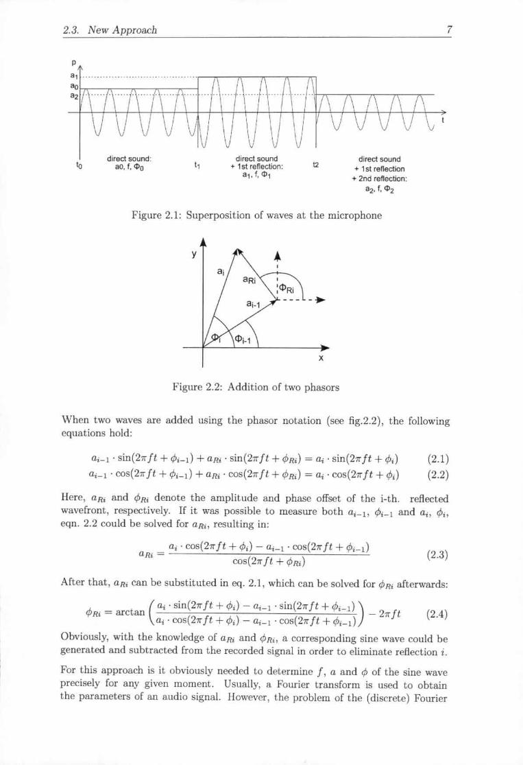
In a room, each single sine wave that contributes to a voiced phoneme will traveldirectly from the speakers mouth to the microphone if no obstacle is in the way.The diaphragm of the microphone will then oscillate due to the pressure variationsof the sound wave. Later, when the first reflected sound wave arrives at the mi-crophone, both the direct sound and the first reflection interfere. Each additionalreflected sound wave, which arrives at the microphone, interferes with those whichhave arrived earlier. Figure 2.1 shows this process in detail.

At t = to, the direct sound arrives at the microphone. Its frequency is J, itsamplitude ao and its phase offset t/Ju. The first reflection arrives at t = t1 and sinceit is a reflection of the direct sound, its frequency is also f. After it has interferedwith the direct sound, the total amplitude is a1 and the total phase offset is tP1' Thisprocess is repeated with each new reflection which arrives at the microphone

2.3. New Approach 7

p

I.........r

VJi

al .

•0

"

direct sound:aO, f, 410 I,

direcl sound+ 1st reflection:

31. f, $112

direct sound+ 1st reflection+ 2nd renection:

32. f. <Il2

Figure 2.1: Superposition of waves at the microphone

y

x

Figure 2.2: Addition of two phasors

\Vhen two waves are added using the phasor notation (see 6g.2.2), the followingequations hold:

a,_I. sin(2nft + ,p.-d + aR'. sin(2nft + ,pR') ~ a;. sin(2nft + <P.) (2.1)ai-\ . cos(2n ft + ,pi-\) + aR' . cos(2n ft + <PR') ~ a; . cos(2n ft + <P.) (2.2)

Here, aRi and et>Ri denote the amplitude and phase offset of the i-tho reflectedwavefront, respectively. If it was possible to measure both ai_I, tPi-1 and ai, tPi,eqn. 2.2 could be solved for aRi, resulting in:

ai' cos(2nft + <Pi) - ai-j •cos(2nft + <p.-daRi =

cos(2n ft + ,pR.) (2.3)

After that, aRi can be substituted in cq. 2.1, which can be solved for et>Ri afterwards:

(2.4)~ (aj' sin(2nft + <P.) - ai-\ . sin(2nft + ,p.-d) f'f'Ri = arctan --~~~--~-~~-~~--~~ - 211' t

a •. cos(2n ft + <Pi) - ai-\ . cos(2n ft + <pi-dObviously, with the knowledge of aRi and ifJRi' a corresponding sine wave could begenerated and subtracted from the recorded signal in order to eliminate reflection i.

For this approach is it obviously needed to determine f, a and ifJ of the sine waveprecisely for any given moment. Usually, a Fourier transform is used to obtainthe parameters of an audio signal. However, the problem of the (discrete) Fourier

8 2. Analysis of the Problem

transform is that it trades temporal resolution for frequency resolution: If the Fouriertransform is calculated based on a long period of time, the output "bins" of theFourier transform are narrow, resulting in a good frequency resolution. If the Fouriertransform is calculated based on only a small amount of samples, its frequencyresolution is bad. For example: If each output "bin" of a FFT should represent afrequency bandwidth of 10Hz, a 480o-point FFT must be used when the sample rateis 48kHz. A 4800-point FFT at 48kHz corresponds to averaging over a timespan ofO.ls. Unfortunately, multiple reflections of a sound wave arrive at the microphonewithin a few milliseconds, not within hundreds of milliseconds. As a result, the FFTmust be calculated based on fewer samples, for example just 48, in order to be ableto measure ai and tPi between the arrival of two consecutive reflected wavefronts. A48-point FFT however, results in output bins which are 1000Hz wide. This is clearlytoo much to separate multiple harmonic frequencies in voiced speech, because theyare usually only between 80 and 200Hz apart.

To solve the problem of the measurement of I, a and tP, phase-locked loops areused in this work. Chapter 3 contains a detailed description of PLLs, for now it isenough to know that they can provide the required precision for the estimation ofthe sound's parameters. Their drawback is that they can only operate on a singlefrequency component, which is why a recorded signal has to be split up into itsfrequency components using bandpass filters and each band of the filter must thenbe passed to a single PLL.

When the parameters JlkJ, alkJ and ~[kJ have been successfully estimated for eachrecorded sample k using a PLL, the actual dereverberation can start by determiningthe frequency 10, amplitude ao and phase offset tPo of the direct sound. For this task,it is necessary to first detect the start of the direct sound in the recording before I,ao and cPo can simply be read out at that instant of time.

After the parameters of the direct sound are knmvn, the parameters of each consec-utive sample can be compared to those of the direct sound using equations 2.3 and2.4. \Vhen the first reflection has not yet arrived at the microphone, the resultingreverb amplitude aR will be close to zero.

However, if a reflected sound wave has arrived and interfered with the direct sound,the reverb amplitude aR and reverb phase <PR will rapidly change to accommodatethe new situation. This change in reverb amplitude and phase can be detected, sothe time tt for the arrival of the first reflected wavefront is known and the combinedamplitude al and phase offset <P1 of the direct sound and the first reflection can beread out at t1. \Vith this information, the correct reverb amplitude aRt and phaseoffset <PRl can be calculated afterwards to produce a copy of the first reverberation,which can then be subtracted from the recording.

From then on, the parameters of all further samples can be compared to al and 91,waiting for a change in reverb amplitude or reverb phase again. This procedure isthen repeated until the end of the recording or until the reverberation amplitudesarc so low that they don't change the sound anymore. This could he possibly thecase for reflections that arrive very late after the direct sound, which means theytravelled a long distance through the air and lost most of their energy on the way.

After the end of the direct sound, the mea.'mroo amplitude and phase offset will stillkeep changing from time to time, hut this does not happen due to newly incoming

2.3. l'lew Approach 9

reflections but due to discontinuing reflections. \Vhen the i-tho reflected wavefrontarrives at the microphone at t = ti, it took tj - to seconds to travel from the speakerto a reflective surface and to the microphone. As a result this very reflection willalso disappear ti - to seconds after the direct sound has ended.

This can be used in the following way: At first, the end of the direct sound must bedetected (for example by detecting the largest drop of the signal energy) and then,it is known that all "reflections" detected later are not new reflections but endingreflections. Because this is difficult to describe, fig. 2.3 depicts what is actuallyhappening.

1.,

'" ""~ 1-'-' "''''''ng1I , ,, ,0.'

, ,,0

-<1,-I

-1.50 0.1 0.2 0.3 0' 0.' 0.6 0.7 06 0.'

1.,I----reve~tionlI

05

0-0.,

-I-1.50 0.1 0.' 0.3 0' 0.' 0.6 07 0.6 0.'

1-recording - revefberation I0

-I

0 0.1 0.2 03 0.' 0' 0.6 0.7 06 0.'time (s]

Figure 2.3: Dereverberation of a single reflection

After t.hedirect sound has ended at t = 0.65s, another "reflection" would be detectedat t = 0.75s due to the ending of the actual reflection. After the end of the directsound has been detected at t = 0.65s, it is known that the direct sound (whichis the target signal for the dereverberation) is zero for t > 0.65s. The additional"reflection" can thus be removed in the same way as the actual reflection by producingand subtracting a corresponding "counter" sound wave.

2.3.2 Extension for a Time-Varying Freqnency

\Vhen the frequency of the direct sound changes over time, equations 2.1 and 2.2do not hold because they assume a constant frequency. However, assuming that the

10 2. Analysis of the Problem

PLL tracks the changing frequency, its value f(t) is known for each instant of time,which allows for the following calculation:

8(t) = a. sin(211"f(t)t + </J)= a. sin(211"(f(0) + "'I(t))t + </J)= a. sin(211"f(O)t + 211""'I(t)t + </J)

" J••••.•(t)

(2.5)

In this equations, /(0) corresponds to the inital frequency of the sine wave, whichit had before the frequency started to change. In situations where the frequency ispermanently changing (like in speech), 1(0) would be the frequency at the beginningof the direct sound.

It can be seen from eq. 2.5 that is is possible to convert a signal with a time-varyingfrequency into a signal with a constant frequency and time-varying phase offset.\Vith this conversion, equation 2.1 and 2.2 can be applied again. As a result, thephase offsets tPi-1 and tPi in equation 2.1 and 2.2 must be replaced by time-varyingfunctions <Pi_l(t) and <Pi(t), respectively. Consequently, the resulting reverb phase4lRi(t) will also be time-varying, but there is no problem with that.

2.3.3 Extension for a Time-Varying Amplitude

\Vhen a reflection is detected in a recorded signal, it is detected because the calcu-lated reverb amplitude or phase change rapidly. However, the calculated amplitudeof the reverb can change for two reasons: Firstly, the change can he really due to areflected wavefront, which has arrived at the microphone. Secondly, it is also possi-ble that the speaker has changed his/her voice, for example to form a new phoneme.Voiced phonemes are characterized by their formants, so two voiced phonemes canhave the same fundamental frequency 10, but they still sound different because theacoustic energy is concentrated on different frequencies. As a result, a change fromone phoneme to another is actually a change of amplitude for each harmonic fre-quency. Such changes of amplitude \\'ould he mistaken for an incoming reverberationby the dcreverberation method.

This brings up the question how an intentional change of amplitude can be distin-guished from amplitude variations caused by reverberations. Luckily, the problemcan be solved by considering all harmonic frequencies at once: The inverse distancelaw (p <X :) [Sengpielll] describes the decrease of amplitude as a sound wave prop-agates away from its source. As it can be seen from the formula, the pressure p(which determines the amplitude) does not depend on the frequency of the sound,so the amplitude of a particular reflection decrea.<;csequally for all frequencies.

If the origin for a change in amplitude is not a reflection but a change in the speaker'svoice, the amplitude of the wrongly calculated "reverb" would not decrease equallyfor all frequencies. Instead, the reverb amplitude which is calculated based on acertain frequency /I would not match the reverb amplitude calculated based on an-other frequency h. If such a situation is detected the algorithm should not attemptto dereverberate the recording but instead, it should adapt to the changing directsound by changing the current reference amplitude.

2.4. Summary 11

Detecting the uniformity of the amplitude decrease is one way to distinguish betweenamplitude variations caused by reverberations and intentional amplitude changescaused by the speaker. The method fails, however, if a reflected wavefront arrivesat the same time than the direct sound of a new phoneme. \Vhile this case probablydoes not happen very often, it might still occur from time to time. However, itis expected that after the beginning of a phoneme the speaker will not change toanother phoneme for some time (unless he or she talks very fast). So, a phonemechange will most likely occur when the early reflections (which have the most energy)are already over. As a result, the amplitude of a reflection that occurs at the sametime as a phoneme change will most likely be low, because the reflection is one ofthe late reflections. As a result of this, the intended amplitude change will be higherthan the amplitude change caused by the late reflection, in which case the intendedamplitude change dominates the reflection.

2.4 SummaryIn this chapter, existing dereverberation methods have been presented like beam-forming using microphone arrays or a blind dereverberation approach. Both of thesemethods have drawbacks which limit their use in real-world applications. This wasthe motivation to develop a new dereverberation method which works using a singlemicrophone and without prior knowledge of the speaker or room.

The theory for the new approach was presented in section 2.3, first for the simplecase of a sine wave with constant frequency, amplitude and phase offset. In thefollowing sections, the theory has been extended to also handle signals with time-,,-arying frequencies or amplitudes, which is needed if the algorithm is ever to beused on real speech signals.

3. Phase-Locked Loops

A phase-locked loop (PLL) is basically a feedback control system, which acceptsa sinusoidal target signal as an input and then matches the frequency and initialphase of a local oscillator to the parameters of the target signal. \Vhen a PLLcircuit has arrived in a state where the local replica oscillation matches the targetsignal (at least to a certain amount), it is considered to be Hlocked" or "in-lock".Furthermore, PLLs can be extended by an amplitude estimation circuit in order tofind the amplitude of the target signal after the PLL has locked.

\Vhen a PLL is in-lock and the amplitude estimator has had enough time to mea-sure the signal amplitude, all parameters of the sinusoidal target signal (frequency,amplitude and initial phase offset) are known to the user of the PLL. The purposeof this work is to find out if this information can be used to track the characteristicsof sinusoidal sounds and their reverberations in a room.

According to (Best93, p. 5], Henri de Bellescize described the first PLL implemen-tations in his work "La reception synchrone" in 1932. Today, PLLs are widely used.in many electronic circuits such a.c;F1"t or GPS receivers, TV sets or frequency syn-thesizers. Because of this, a lot of literature covering different aspects and use-casesof PLLs is available. Some of the standard works about PLLs are "Phase-LockedLoops" by R. nest [ncst93J and "Phaselock Techniques" by F. Gardner [Gardner05J."Phase-Locked Loops for \Vireless Communications" by D. Stephens (Stephens02J isanother book which - despite its name - also contains PLL basics and comprehensivemathematical descriptions of both single PLL components and PLL systems as awhole.

The goal of the following chapters is mainly to mathematically describe the PLLsystem which wa.c;used for this work. At the same time, an introduction to PLLs isgiven which also explains the basic working principles and the components PLLs aremade of. Neither will the following chapters cover all types of PLLs, nor are theyintended to give a comprehensive mathematical description of all aspects of PLLtheory and design. The behavior of a PLL will only be discussed in detail for thesituations where the PLL has already locked. ~1athematical analyses of the unlockedstate make use of nonlinear differential equations, for which no exact solution ha.c;been found until today [Best93, pp. 25J. In the textbooks mentioned above, usually

14 3. Phase-Locked Loops

some approximations are made (such as sin (x) :=:::: x for small values of x) to be ableto solve the equations. i\cvertheless, findings derived from these approximationshave proven to be reasonably valid so they will also be used in latcr chapters.

3.1 Types of Phase-Locked LoopsBefore looking at the individual components a PLL is made of, it is importantto know in which ways a PLL circuit can be implemented at all. In [Bcst93, p.6 and further chapter introductions], the author R. Best describes four t:ypcs ofPLLs: analog PLLs (APLLs), digital PLLs (DPLLs), all-digital PLLs (ADPLLs)and software PLLs (SPLLs).

APLLs are also called linear PLLs in [Best93], hence another abbreviation for themis LPLLs. However, the term APLL will be used for an analog phase-locked loop inthis work. As the name suggests, APLLs are built solely out of analog circuit com-ponents, such as capacitors, resistors, inductors and the like. As it is the case withall analog components, these parts suffer from production tolerances and spread,which would have to be taken into account if one wanted to be really precise. Theyare also not well applicable for experiments because it \vould be necessary to replacecomponents and to rewire them for each new parameter setting. Their advantage isthat they are not subject to the Nyquist sampling theorem and as a result of that,APLLs can operate on signals with very high frequencies \\Tithout using expensivefast analog-digital converters.

ADPLLs on the other hand are built completely out of logical circuits like countersor flip-flops. ADPLLs can either operate on binary digital signals (square waves)or on discrete, digitally sampled analog signals, i.e. data words. A drawback of alldigital systems is of course the effect of the sampling theorem which results in thefact that only signals with frequencys below ~ . f8ampling can be processed in an AD-PLL. Additionally, sampling errors always arise when working with sampled analogsignals. Like APLLs, classic ADPLLs are also built in hardware which reduces theirsuitability for experiments. However, reconfiguring an Ie is easier than solderingnew components on a printed circuit.

DPLLs are a combination of APLLs and ADPLLs, having some digital parts mixedwith analog parts. Depending on \\Thichparts are digital and which are analog, theymight have some of the (dis)advantages of APLLs and some of ADPLLs.

The last type of the four are software PLLs. As the name suggests, these PLLs arefully realised as software components and as such they can be programmed to act likeany of the other PLL types, given the sample rate is high enough to fulfil the samplingtheorem. They can easily be reconfigured or reprogrammed to suit different needswhich makes them ideal for simulations and research. Furthermore, it is possible touse parts and operations in an SPLL which cannot be built as an analog circuits, forexample the trigonometric functions. Depending on the complexity of a PLL designand the computer hardware used to run the software, execution can be slow and notsuitable for real-time operation, even on modern computers.

For this paper, an SPLL system based on an analog PLL ha.';;been implementedusing rvlatlab and Simulink from The Mathworks, Inc. Some of the reasons for thisdecision have been:

3.2. Components of a PLI.. 15

• The system can be implemented and tested without buying hardware andbuilding actual circuits .

• Campus licenses for )'latlab and Simulink are available free of charge at theKIT software shop .

• The PLL can be easily reconfigured to test different configurations and param.eters .

• Additional components can be built in easily.

• Many audio test files can be processed automatically and evaluated usingscripts .

• Simulink models can be automatically compiled to create programs for com-mercially available FPGA or DSP microchips.

3.2 Components of a PLLFig. 3.1 shows the three basic components of a PLL system:

u1~ephase loop--. detector filter

u2local

oscillator

Figure 3.1: diagram of a classical PLL circuit

The target signal has a sinusoidal shape and it is denoted by Ul. The local oscillatoroutputs another sinusoidal signal, which will be named U2 hereon. !\.lathematically,these signals can be described as follows:

",(I) ~", . sin(27rj,t + <I,) (3.1 )

u,(t) =",. sin(27rf,t + 1>,) (3.2)

Ul and U2 are compared in the phase detector and the output of an idf'~l phasedetector would be tPe = rPl - 1>2' 4>e is called phase error or phase difference betweenUl and U2. The phase error is then usro as an input for the loop filter, which isfor example a lowpass filter. The design of the loop filter is most crucial for theoperation of the loop, because it determines the amount of signal noise a PLL canhandle or the time it takes, until the PLL gets locked. The output of the loop filteris a control signal, which is used to increase or decrease the instantaneous frequencyi2 of the local oscillator's sinusoidal output.

16 3. Phase-Docked wops

In traditional PLLs, only the frequencies 11 and h as well as the initial phase offsets<PIand ih match when the PLL is locked. However, the amplitudes a} and U2 arenot equal and as a result, the PLL input Ul (t) and its output udt) a.re not equal,too.

Usually, the local oscillator produces a sine wave with a default amplitude of U2 = 1,whereas the amplitude of the waveform stored in a ,wav audio file is within theinterval [0,11, depending on the sound volume. As it was shown in chapter 2, sig-nal amplitude is an important property when tracking reverberations in an audiorecording, hence it needs to be estimated. This can be done by an additional am-plitude estimator, as seen in fig. 3.2. The additional circuit estimates ail so it canbe multiplied by the replica signal (whose amplitude a2 equals 1) later. It can beseen in the diagram that the amplitude estimator is not part of the actual loop, so itdoesn't contribute to the behavior of the loop in terms of control theory. As a result,the explanation of the amplitude estimator will be given at the end of chapter 3 insection 3.5.

"1 ~.phase loop- detector filter

al amplitude ..- ", localestimator oscillator

Figure 3.2: diagram of a PLL circuit including an amplitude estimator

3.2.1 Phase Detector

As already stated, the phase detector (usual abbrev.: PO) calculates the phaseerror of the two signals Ul(t) and U2(t) (fig. 3.1). A very common phase detector(for APLLs), which is presented and analyzed in many books about PLLs, is themultiplying phase detector. In the next section, the multiplying phase detector willbe analyzed and the reason why it has not been used will be presented.

For the analysis of any PO, it is assumed that the frequencies Ii and h alreadymatch, so the ideal output of the phase detector would simply be 4Je= cPl - 4J2. Asit can be seen in the next section, the output of the multiplying phase detector israther different so the Hilbert Phase detector will be introduced in the next but onesection to have an alternate solution.

3.2. Components of a PLL 17

3.2.1.1 Multiplying Phase Detector

As the name suggests, the multiplying PD simply consists of a multiplier whichcalculates the product u,(t). u,(t). This yields the following result:

u,(t) . u,(t) ~ a, . sin (2nIt + 4>tl . a, . sin (2nIt + 4>,)

. (4nIt + 24>,+ 4>,- <h) . (4nIt + 24>,+ 4>,- 4>,)= al • a2 • sm 2 . sm 2

. (<>+/3) . (<>- (3)= al . a2 . sm -2- .sm -2-

In the last line, the substitutions 0: = 41rft + rPI + rP2 and {3= <Pl - <P2 have beenmade, because after that it is possible to apply the following trigonometric identity:

(<>+ (3) (<>- (3) 1sin -2- .sin -2- =-2.(cOSO:-cos,B)

After applying the identity and re-substituting the values for 0: and ,B, the result is:~- )))u,(t) . u,(t) ~ --2- . (cas(4n It + 4>,+ 4>, - cos(4), - <hala2 a}a2 )

~ -2- . cos(1" : <h)- -2- . cas~ t + 4>,+ <h<Pe double frequency component

(3.3)

As it can be seen from eqn. (3.3), multiplying both signals does not directly resultin <Pebut rather in the cosine of it as well as another cosine component having twicethe frequency of the target signal. The first thing to do is to filter out the doublefrequency component using a lowpass filter. This filter must not be confused withthe actual loop filter, although a loop filter could be designed in such a way, that italso filters out the double frequency component.

At first, the lo\\-pass filter does not seem to be a huge problem, unless one recalls thatthe PLL design in this work is intended to operate over the whole frcqency spectrumof human speech. Because of this, it has to work at input frequencies of about 100Hzas well as, for example, 2kHz. At 2kHz, the lowpass filter should therefore eliminatefrequencies of 4kHz and above. If the same lowpass filter was used for an inputsignal of 100Hz, too, it would obviously not be able to remove the double frequencycomponent at 200Hz. Because of the fact that a PLL can only track one frequencyat once, many PLLs will be used to track each harmonic frequency in speech. \Vithmultiplying phase detectors, each of these PLLs would need a specifically designedlowpass filter. This is one of the reasons why the multiplying phase detector wasnot used.

\Vhen Fww denotes an appropriate lowpass filtering operation, the result is

ala2Fww{u,(t). u,(t)} '" -2-. cos(<P,)

=> <P,'" arccos (_2_. Fww(u,(t) . ",(t)))ala2

(3.4)

(3.5)

18 3. Phase-Locked Loops

~ow the biggest drawback of multiplying phase detectors gets obvious: As one cansec, the right hand side of equation 3.4 depends on al and a2. The factor a2/2 isdown to the local oscillator (usually, a2 = 1) and the PLL designer can thereforecompensate for it. at. however, corresponds to the power of the target signal, whichis probably not known by the designer (depending on the use-case of the PLL).Therefore, the multiplying phase detector yields an undesirable behavior when thepower of Ul changes. So, if it cannot be guaranteed that at is constant (like inrecordings of human speech), some sort of automatic gain control (AGe) needs tobe used [Stephens02, p. 19] in order to keep at at a certain known value.

3.2.1.2 Hilbert Phase Detector

The Hilbert phase detector works on digitally sampled versions of analog signals, soit is best used in an ADPLL or SPLL. Descriptions of this detector can be found forexample in [Stephens02, p. 270J, which refers to [Best93, p. 1861. The name of theHilbert Pha..:;edetector comes from the Hilbert transform, on which it is based. TheHilbert transform (invented by the mathematician David Hilbert) will be denoted by1{ from now on. It is an operation which shifts the phase of all frequency componentsof a signal individually by -1r /2 radians, i.e,

1i{sinx} = -co,x

For the Hilbert phase detector, both the signals Ul and U2 must be manipulatedusing a Hilbert transform which leads to the signals UI and U2, respectively:

UI(t) = al . sin(wll + 'Pt)

UI(I) : = 1i{UI(t)) ~ al . sin (WI I + "'I - ~) = -al . eos(wl I + "'I)

u,(I) = a,. sin(w,1 +",,)u,(I) := 1i{u,(I)} = a,. sin (W,I + "" - ~) = -a,. cos(w,1 + ",,)

(3.6)

In these equations, it and h have been removed by the substitution Wi = 21r Ii tomake the equations easier to read. Like for the analysis of the multiplying PD,WI = W2 = w is assumed, so the desired output of the phase detector is cPe = <PI - tP2'

\Vithin the phase detector, the following operations are performed:

S;9,(I) := UI(t). u,(I) + UI(t). u,(I)= ala,. (sin(wl + "'I)' sin (wi + ",,)+ eos(wl + ",,). cos(wl + "',))

Using the substitutions 0 = wt + 4>1 and {3 = wt + th. and the trigonometric identitysin o. sin {3+ cos 0' cos 13= cos(o - 13), this equation can be transformed to

S;YI(t) = a,a,. cos (wi + "', - (wi + ",,))= alu2' COS(cPI -~)

= ala2' cos(tPe) (3.7)

3.2. Components of a PLL 19

Eq. 3.7 still depends on the input amplitude al and on its own, it would thereforebe of no more use than the multiplying phase detector. However, another signalcombination can be produced:

si9,(t): = UI(t). u,(t) - UI(t). u,(t)= -ala,. (sin(wt + <PI)' cos(wt + q,,) - cos(wt + <PI). sin(wt + q,,))= -ala,. sin (wt + <PI - (wt + ",,))= -ala,. sin (<PI- q,,)= -ala, . sin(<p,) (3.8)

For this conversion, the arguments of the trigonometric functions can be substitutedby Q and {3again, before applying the identity sin 0:' cos 13- cos 0:' sin 13= sin(o: -13).

After that, si!h(t) is divided hy si9I(t), which results in:

si9,(t)si9l(t) (3.9)

As sig2 is divided by Sigh the result gets independent of any signal amplitudes.Additionally, the Hilbert phase detector does not need an additionallowpass-filteringlike the multiplying phase detector.

Besides the needed arctan function, which can easily be implemented in software,the only remaining difficulties in the implementation of the Hilbert phase detectorare the actual Hilbert transforms needed to produce Ul and U2. However, there arelocal oscillators which produce not only a sine wave (U2) of a given frequency, butalso a corresponding cosine wave. This cosine wave can simply be multiplied by -1to get the Hilbert transform of the sine wave, i.e. U2.

As a result, only UI must be calculated by a Hilbert transform effectively. The actualimplementation of a Hilbert filter will be discussed in ch. 4.1.2.

3.2.2 Local Oscillator

The local oscillator of a PLL has to generate a sine wave with a certain instantaneousfrequency (and also a cosine wave at the same frequency if a Hilbert phase detector isto be used). In APLLs, the local oscillator is typically a voltage-controlled oscillator(VCO). This means, that the voltage applied at the input of a veo determines theinstantaneous frequency of its output. As the SPLL presented in this work resemblesan APLL, a discrete-time veo has been used. This is simply a VCO whose outputis digitally sampled at a certain sampling rate. Other PLL implementations mightalso feature a current-controlled oscillator, for example, but this depends on theapplication the PLL is used for.

In addition to the discrete-time veo, Simulink also provides a so-called numerically-controlled oscillator (NCO), which can he used (almost) like a VCO. Mathematically,they should both perform the same task and so the formulas describing the discrete-time VCO should also fit the KCO. In the Simulink NCO block, the sin function isrealized using a precalculated lookup table, which stores the result of sin (x) for anygiven x. This way of calculating trigonometric functions is usually faster than using

20 3. Phase-Locked Loops

(3.10)](t) = ~ dB211" dt

the respective functions from a software math library, which is what the discrete-time veo block does. Additionally, the amount of entries in the lookup table canbe controlled explicitly, which allows/forces the designer to decide between memoryconsumption and mathematical precision. However, Simulink's ~CO block has notbeen used in this work, because there is possibly a flaw in its implementation, whichwill be explained later, after the mathematical description of a veo.A veo in Simulink has only one input port and the value Uin(t) applied at itdetermines the instantaneous frequency of the sinusoidal veo output. In a realphysical circuit, the unit of the input would be volt, so it makes sense to specifythe sensitivity (or gain) K. of a veo in 1[,z. Thus, "'0 controls by how many Hz theinstantaneous frequency of the output changes when Uin is changed by one (volt).

The behavior of a veo can be further adjusted by another parameter, 10[= Hz]. Itis called the quiescent frequency and it specifies the veo output frequency for aninput of ov. In some applications, for example in FM demodulation, where there isa known carrier frequency III 10 can be set to It. As a result, the PLL only has tocontrol the phase shift of the veo output in these cases, but not its frequency.

Given specific values for KQ and 10 and a certain function Uin(t), the purpose of theveo is to produce a sine wave with an instantaneous frequency j(t) = 10 +KQUin(t).By definition, the instantaneous frequency ](t) of a sinusoid like 9(t) = sin(B(t)) isthe derivative of its phase:

Thus, it is not sufficient to simply calculate U2(t) = sin(21r(Jo+Kuin(t) )t) in the yeo.Using eq. 3.10 and the product rule, the instantaneous frequency of the resultingsine wave would be:

Obviously, this is not the desired output of j2(t) = 10+ K.Uin(t). To obtain thecorrect output, the calculation in the veo must be:

U2(t) = siu (211" l~dt+q,o) (3.11)

i2(t)

Deriving the phase of eq. 3.11 by means of eq. 3.10 yields the proper value for theinstantaneous frequency, so eq. 3.11 is the correct equation for a veo.

In the beginning of this section it was mentioned that the Simulink NeO and veoblocks differ. One of these differences is that the veo block implements eq. 3.11directly, i.e. the input to the veo is actually Uin' The :"Jeo block, however, doesnot expect Uin as its input, but 12 = fo + 1Win- As a result, 12 would have to becalculated outside of the KeO block.

In eq. 3.11, </>0 is an optional (constant) initial phase offset for the veo sinusoid.Since the initial phase offset <PI of the target signal is not known, it is impossible toset the yeO's initial phase offset mo close to mi, Thus, </>0 can be set to 0, because

3.2. Components of 11 PLL 21

o is no better or worse choice than any other value. \Vith this, eq. 3.11 can betransformed as follows.

u,(t) = sin (2rr 1.' fa + Kum(t)dt + 0)= sin (2rr 1.' fodt + 2" 1.'KU.n(t)dt)

= sin (2"fot+2" l'KU.n(t)dt),0 ,

voh(t)

(3.12)

Obviously, 'U2 can be seen as a sine wave at a frequency of fo Hz and with a changingphase offset of 4>2(t) radians. Now, it is important to recall the purpose of a PLL:A PLL is ought to be a servo loop for the phase of the veo output signal. As aresult, the important property of eq. 3.12 is not the actual resulting signal U2(t), northe instantaneous frequency f~(t), but only the phase offset <P2(t). This is the onlyinformation that matters in the phase detector afterwards.

Eq. 3.12 models the veo output in time domain, but as the goal of this work isto build a digital feedback control system, it is important to know the z-domaintransfer function of each component. In section 3.3, these transfer functions willthen be used to analyze the stability of the feedback control system.

+ Sin

Figure 3.3: Simplified diagram of the Simulink discrete-time veo block

Figure 3.3 is a simplified schematic drawing of the internals of a (Simulink) yeo.Obviously, for every sampling step, t.he integration result is calculated as the sumof the integration result from the previous sampling step plus the input to theintegrator from the previous sampling step. Before adding the current input to thetotal sum, it has to be scaled by T8 (the sampling time), because otherwise changingthe sampling rate would also change the result of the integration. For instance, ifthe sampling rate was increased, the yeO input would be added to the sum moreoften in a given period of time, which would lead to a wrong result. Accordingto [Stephens02, p. 216], this kind of discrete integration is also known as "ForwardEuler" integration (in contrast to "Backward Buler" integration, where the delayblock would be placed in the backward part of the loop).

As an equation, the integration in fig. 3.3 looks like:

integratorout[tj = intcgratorout[t -IJ + T8 • integratorin[t - IJ

22 3. Phase-Locked Loops

Here, t specifies the index of the sampling step, so t - 1 corresponds to the samplingstep just before step t. Now that the integration method is known, the z-domaintransfer function Fvco[z] can be derived. As stated before, only the pha..o;;e offsetrP2(t) is important, so 10 must not be taken into account in the transfer function.

<I',[z] ~ z-I<I',[z] + 2""T, . Z-IUin[Z)<1',[,] - z-I<I',[z] = 2""T, . ,-IUin[Z)

,~,[z)(1 - Z-I) ~ 2""T, . Z-IUin[Z]<I',[z] ,-I

FvGa[z] := -U [ ] = 2""T, -IinZ l-z

(3.13)

This result differs from the equation given in [Stcphcns02, p. 216, eq. 7-57] by afactor of 211'""'; due to the fact that the Simulink KeD expects the unit for the inputto be Hz rather than radians and Stephens has not included the gain K in the transferfunction for the digital veo, as opposed to the analog yeo.

3.2.3 Loop Filter

From the three components of a classical PLL, the phase detector and the localoscillator have already been discussed in the previous sections. This section willtherefore cover the loop filter. However, before covering specific filter designs, thedefinition of the order of a PLL must be given.

3.2.3.1 PLL Order

In terms of control theory, a PLL in total can be regarded as a servo loop for thephase of the incoming target signal. As a result, it is possible to set up a transferfunction which describes the effect the loop has on the phase of the target signal.This will be done in chapter 3.3.

For now, it is enough to recall eq. 3.13 from chapter 3.2.2. The transfer functionof a veo has one pole for z = 1, so the order of the veo's transfer function isone. \Vith respect to control theory, the phase detector realizes a negative feedback,because its output is l/Je = l/Jl - tP2. It does therefore not introduce any further polesto the system as a whole.

As a result, the total order of the PLL is determined by the order or the loop filterplus one for the pole of the veo. A PLL will consequently be considered a nth orderPLL if the order of the loop filter is n - 1.

According to [Stephens02, p. 16-18], loop filters of order zero, i.e. simple linear gainfactors, manage to adjust the phase offset tP2 of the local oscillator if the initialphase offset of the target signal follows a step function. Thus, when 4>1 changesto another value instantaneously, cP2 will get equal to 4Jl after a certain amount oftime. However, PLLs with zero order loop filters cannot compensate input changesof higher order, which means that zero order PLLs are not able to follow the targetsignal if the change of <PI can be described by a ramp function, a quadratic equationor any polynomial of even higher order.

On page 29 of [Stephens02}, the author explains that by increasing the order of thepha.'iC locked loop, "it tends to compensate for an instantaneous change in the next

3.2. Components of a PLL 23

higher derivative of the input". For example, PLLs of order hvo are able to follow thetarget signal even if its initial phase offset is constantly increasing [Stephens02, p. 38].According to eq. 3.10, a linear variation of the target signal's phase offset amountsto a step change of its instantaneous frequency. This can be seen in fig. 3.4(b) onpage 24.

Phase variations of the next higher order can be described by quadratic equations,so by using C<}. 3.10 again, they are equal to a linear ascent of the target signal'sfrequency, as depicted in figure 3.4(c).

At first sight, it seems desirable to increase the order of a PLL as much as possiblefor the tracking of harmonic frequencies in human speech, so it can follow eventhe most complex input characteristics. However, by looking at the filter designequations following in section 3.4, it can be seen that a specific design of a PLL isalways a trade-off between tracking stability and tracking speed. So, using a higherfilter order makes the loop more stable when the input changes slowly, but it alsoincreases its reaction time, which might render the loop too slow to follow the fastfrequency changes occming in human speech. Another drawback of high order loopsis the increased computational load, which should usually be kept low.

The biggest problem is finally not the computational load, but the complexity ofthe filter design. For 1st order loop filters, the filter coefficients can be calculatedby equations which have a real physical meaning, like for example the time it takesfor the PLL to lock or maximum signal-to-noise ratio at which the PLL can lock atall. Loop filters of order two and higher must be designed by parameters withouta direct physical meaning, like the filter's phase margin, its unity gain crossoverfrequency or the position of the filter's poles in a root locus plot. On page 103of [Stephens02], the author even suggests iterating some design parameters until agood result is achieved.

As a result, 15t order loop filters have been used in this work. The equations whichcan be used. to specify their parameters will be presented in section 3.4, after thetransfer functions for both the loop filter and the PLL as a whole have been derived.

3.2.3.2 First Order Loop Filter

There are many ways how a first order loop filter can be designed, for exampleas a simple first order lowpass, as a passive lead-lag filter or as an active lead-lagfilter [Stephens02, p. 311.For this work, the ""tive lewl-lag filter (= PI controller)has been chosen, because a loop with an active lead-lag filter has an infinite pull-in range (Best93, p. 41]. This means that such a PLL can theoretically lock ontoany frequency, no matter what the current instantaneous frequency i2 of the veois. Depending on the frequency offset /).,1 = il - i2' the locking process mighttake some time, but sooner or lat.er the PLL will get locked. PI is actually anabbreviation for ''proportional and integrating", which means t.hat the output of thefilter depends both linearly on its input but also on the integral of its input overtime. This integrating characteristics allows the output of a digital PI controllerto increase infinitely (at least theoretically, as long as there is no overflow in anyvariable), which, in turn, allows for an infinite pull-in range. On the other hand,PLLs with first order lowpass filters or passive lead-lag filter have limited. pull. inranges.

24 3. Pha.<;e-Locked Loops

t

t

.--,

Jj

t

M

t

(a) phase step (b) frequency step = phase ramp

Jj

t

(c) frequency ramp

Figure 3.4: Possible characteristics of a PLL input.

3.2. Components of 8 PLL

R, R,c

25

(3.14)

Figure 3.5: Schematic diagram of an analog PI-controller IBest93, p. 8].

•2OdB/decade

Ol

Figure 3.6: Frequency response of a PI controller (logarithmic axes). In theory, thefilter gain is infinite for w = O. Figure is based on !Best93, p. 9j.

Figure 3.5 shows the components of an analog PI controller and fig. 3.6 its frequencyresponse curve. Obviously, there are 3 design parameters in the circuit, namely theresistors RI, 112 and the capacitor C. Luckily, when the circuit is converted to ans-domain transfer function, these parameters can be combined to TI = RI • C andTZ = llz . C, which results in two degrees of freedom for the designer. The transferfunction of a PI controller can be found for example in [Best93, p. 10J and it is:

1+ T2SF(s)=--TIS

There are several possible ways of converting a transfer function from s-domain toz-domain, like the impulse-invariant z-transform or the bilinear z-transform. Whilethe impuls-invariant z-transform ensures that the impulse response of the resultingdigital filter resembles the analog impulse response as much as possible, the bilinearz-transform allows the digital frequency response to match the analog frequencyresponse better. The following substitution must be done in an s-domain transferfunction to get the equivalent z-domain transfer function:

2 1 - z-Is=-----

T8 I+ z-l (3.15)

26 3. Phase-Locked Loops

\Vith this substitution, the z-domain transfer function of a loop filter that has theform of a PI controller can be derived as follows:

1 2 1_,,-1+ T2T. 1+:-1FLP[z) = 2 1_,,-1

71 T. 1+:-1L. l-z-12 +T2~

l-z ITl1+r11 T.(I+r1) + (1- -I)

Hz-I 2 72 Z

= l+~-I . Tl(1- Z-l)

:r. + 1iz-1 +"" _ To Z-l2 2 '2 2

TI(I-z-I)

1i..+ !l + (L.. _ !l) Z-I2n 1"1 2T} Tl

1- Z-l(3.16)

Unfortunatc1y, transforming an analog filter to a digital one by means of a bilinearz-transform changes the corner frequencies of the resulting digital filter. The reasonfor this is, that the bilinear z-transform maps the whole (infinite) frequency rangeof the analog filter to the (digital) frequency range [0, -1). where f~denotes thesampling rate of the digital system. Low frequencies, which are far away from It,arc mapped (more or less) "exactly", but the closer a frequency is to ~, the biggerthe mapping error gets.

If the corner frequencies of the resulting digital filter should match those of thecorrcsponding analog filter, a procedure called "prewarping" has to be done beforethe filter is transformed by the bilinear z-transform. To prewarp a given filter, allof its corner frequencies Wi must be transformed by cq. 3.17 {Dest93, p. 348]. Thismoves all corner frequencies in such a way, that the corner frequencies of the resultingdigital filter equal their analog counterparts.

From fig. 3.6, it can be seen that the only corner frequency of a PI controller isdetermined by ~. Using eq. 3.17 yields:

1 2 (1 T,)T2,prewarped = T$ tan T2'"2

T2.p'~Mpffi = T() (3.18)2tan :Ii2"

Until now, the transfer functions of all individual components of a PLL have beenexamined. These transfer functions will be combined in the next section to get thetransfer function of a PLL as a whole. After that, in chapter 3.4, a set of equationswill be prescnted which can be used to specify the loop filter parameters Tl and 72.

3.3. Transfer Function and Stability Analysis

3.3 Transfer Function and Stability Analysis

27

To create the z-domain transfer function of a PLL as a whole, it is almost sufficientto simply combine the transfer functions of the phase detector, the loop filter andthe VCO like the model of fig. 3.7 suggests. However, one problem is arising fromfig. 3.7: for any given sample index t, <P2[tj depends on <Pe[t), which, in turn, dependson 4'2[tl. To deal with this problem, a one-sample delay should be inserted in thefeedback loop, so that ,P,[t] docs not depend on itself, but nn <hit - 1).

<PI ~IFvco Q

Figure 3.7: Z-domain block diagram of a PLL.

Luckily, it can be seen from fig. 3.3, that there is already a delay in the forwardlooking part of the Forward Euler integrator in the VCO, so <P2[tJ actually dependson <Pelt -1]. In a Backward Euler integrator, the delay would be part of the VCO'sba.ckward looking signal path. So, with a Backward Euler integrator, an additionaldelay block would be needed somewhere in the loop. This would effectively turn theBackward Euler integrator into a Forward Euler integrator, as it is pointed out in[Stephens02, p. 216/217].

Including an additional delay would actually not be any problem at all, so why isthis issue mentioned here in detail? At first, the simulations for this work have beendone with a Simulink NCO block. By looking at its help page in Simulink, it can beseen that it also features a delay in the forward looking signal path, which is why itcan be considered a Forward Euler integrator. However, when a simulation was triedto be started, Simulink always reported an error occuring from an "algebraic loop".For some unknown reason this could be fixed by adding another delay block, butthen again more delays as actually needed make the system slower as it could be. Inthe end, the NCO was replaced by a discrete.time VCO block, which provides thesame (mathematical) functionality as the NCO, but does not require an additionaldelay.

\Vith the help of fig. 3.7, the z.domain transfer function can be obtained easily:

"',lzJ ~ Fvcolz], FLFlz). "'.[z]= Fvco[z). FLF[Z]' ("'I[zl- "',[z])~ Fvco[z] . FLFlz] . "'1 [z]- Fvcolz] . FLF[Zj. "',Iz]

=> "',Iz] + Fvco[z] . FLFlz) . "',[zJ = Fvco[z) . FLFlz]. "'Iiz)=> "',[zJ . (1 + Fvcolz). FLdz)) = Fvcolz]. FLF[Z]' "'Iiz]

In the standard form Flz] = o;:.~t:t.z l this looks like:

FPLdz] :~ "',[z] ~ Fvcolz)' FLdzJ"'Iiz] 1 + Fvco[zJ . FLdzJ (3.19)

28 3. Phase-Locked Loops

:'-Jow,Fvco[z] and FT.F[Z] can be substituted by eqs. 3.13 and 3.16, respectively:

----L::::::::' 21rK,T . (1L. + !l + (..L.._ !l) Z-I) Z-I~ ~2nTI 21)1)

= --¥) . (1 - Z-I)2 + 21rKT . (L... + !2.+ (L... _ Xl) Z-I) Z-I~_l)l If 21"1 T) 2T1 1)

2JrKTIJ• ((L.. + n.) Z-l + (L. _ .!l) z-')21'} 1) 2TI TI

1- 2z-i + Z-2 + 27rf"T . ((.n.. + Zl) Z-l + (L._ !l) z-,)If 21)1'1 2n1)

(1rf\T; + 2JrKT2Ts) Z-l + (7fK:r; - 21rKTZTll) Z-2-

Tl + (1rKTf + 21rKT2TIJ - 271) Z-l + (1fKT; - 27rK,TzTIJ + Tl) Z-2

The terms in parenthesis can be be substituted now to make the function morehandy. After that, the location of the poles can be determined by setting the de-nominator to zero and using the quadratic formula.

a:= lI"KT;b := 21rKT2Ts

o ! T, + (a + b - 2Tl)Z-1 + (a - b + T,)Z-'

=z'+ (a:,b -2)z+ (a;.b +1)a+b (a+b)' 2a

::::}ZI/2 = 1- ~ :i: 4Tf 7}

(3.20)(3.21)

(3.22)

So, after choosing a sampling time T" a VCO gain K and filter coefficients 71 and T2,

their values can be used in equation 3.22 to determine the position of the transferfunctions' poles. A digital control circuit is stable, if all the poles of its z-domaintransfer function are within the unit circle. Thus, the PLL will be stable, if theabsolute value of its poles is smaller than 1. At this point, the la..•t remaining taskin the implementation of a PLL is to specify its filter coefficients, which will be donein the next chapter.

3.4 Design Equations for 2nd order PLLs

In chapter 3.3, the transfer function for a PLL was established in the z-domain.\Vhen the transfer function is calculated in the Laplace-domain, it looks like this:

211"1<!;/; S + 271"1<

F ()_ T\ T\PLL S - 82 + 211"1<!;jl,<; + ~,., T,

3.4. Design Equations [or ?d order PLLs 29

The denominator of this transfer function can be converted to the standard form of82 + 2Cwns +w~by the substitutions 3.23 [Best93, p. 18]. Wn is called the naturalfrequency and C is called the damping factor.

w. = J27rK WnT2(3.23)(~-

Tl 227rK 2(

(3.24)=> Tl =-- T2= -w' w••

In the following paragraphs, equations from [Best93] will be presented, which canbe used to specify Wn and C. These, in turn, can then be used to calculate the filtercoefficients. Obviously, Wn and ( are defined ba."ed on the analog transfer functionand so will be the equations used to actually calculate these parameters. Estimationsobtained from APLLs are not directly applicable for digital PLLs, but this problemwill be dealt with in section 3.4.3. There, it can be seen that an SPLL behaves likethe corresponding APLL if its sampling frequency is high enough. Unfortunately,the sampling frequency must be a lot higher than the "usual" value of two times themaximum frequency occuring the system.

At first, the parameter ( will be chooen and according to [Best93, p. 19-231, it is bestto select ( = ~ :::::::0.707. For higher values of ( the damping is too high and thePLL reacts too slowly. For smaller values of C the loop is not damped enough, so itreacts too fast and the PLL is affected too much by noise and other disturbances.

Now, as ( has been chosen, Wn is the only free parameter left. There are severalpossibilities to specify Wn' An overview of all APLL design equations can be foundin [Best93, p. 58/59] and three of them will be presented in the following sections.

3.4.1 Design by Pull-Out Range

If a PLL is locked onto a certain frequency, the pull-out range .6.wPo(= 2rr.6.jpo)is defined by [Best93, p. 42/43] as "that frequency step, which causes a lock-out ifapplied to the reference input of the PLL". On the same page in that book, thepull-out range is approximated by

t;wpo '" 1.8w.(( + 1)7r.t;jpo

w -• - 0.9((+ 1) (3.25)

So, by specifying .6.fpo, Wn can easily be obtained and with that, eq. 3.24 can beused to specify the filter parameters. However, because the frequency transitions inhuma.n speech are mostly continuous, it is hard to actually define .6.fpo. This is thereason why the filter parameters have not been defined by the PLUs pull-out rangein this work.

3.4.2 Design by Lock Range

The lock range .6.wd= 21r.6.fd of a PLL is defined as follows: if the local oscillatorcurrently produces a sine wave at a frequency of Wo rOO/s (this can be its quiescentfrequency, but is docs not need to be) and the target signal has a frequency ofWI = Wo + .6.WLrad/s, what can the maximum value of .6.wL be, so that the PLL

30 3.Phase-Locked Loops

locks within one beat-note between Wo and WI? IBest93, p. 38] gives the value forthe lock range as follows:

(3.26)

Eq. 3.26 is useful especially for the design of a rnulti-PLL system. As the voicedparts of human speech are made up of a fundamental frequency f and its harmonics2f, 3f, etc., multiple PLLs are needed to track all of the frequencies. To accomplishthis task, the target signal is split into many frequency bands using band-pass filters.Because the bandwidth of the band-pass filters is known, equation 3.26 can be usedto build a PLL which is able to lock onto any frequency in its frequency band withinone beat-note.

3.4.3 Design by Noise Bandwidth

The target signal for a PLL is ideally a perfect sine wave at only one certain fre-quency. However, if there are other frequencies present in the input signal, the PLLwill still try to lock on the frequency component with the highest amplitude. Indoing this, frequencies of lower amplitude are suppressed and as a result, the VCOoutput signal has an increased signal-ta-noise ratio compared to the PLL input.

\Vhen noise is added to the target signal, the zero crossings of the target sine functionwill be displaced forward or backward in time !Best93, p. 47]. This means that noiseof a certain bandwidth induces phase jitter, which will be reduced by the PLL.According to [Best93, p. 49], the following equation holds:

B(SNRh ~ (SNR) •. -B'

2 L(3.27)

In this expression, (SN R)i and (SN R)L denote the signal-ta-noise ratio at theinput of the PLL and at the VCO output, respectively. These values are calculatedusing the frequency noise and not the phase noise. Furthermore, the (double-sided)bandwidth of the noise at the input is supposed to be Bi and BL is called the loopbandwidth or noise bandwidth. As an example, if a frequency of 1000Hz is to betracked by a PLL, but there are further, equally distributed, frequency componentsfrom 950Hz to 1050Hz in the target signal, Bi would he 1050Hz - 950Hz = 100Hz.Dividing the signal power of the 1000Hz component by the rest of the power withinthe range from 950Hz to 1050Hz yields (SN Rk Concerning (SN Rh, experiencehas shown that it has to be at lea..<;t4 (= 6dB), otherwise the PLL will not he workingstably [Dest93, p. 501.

From the variables of eq. 3.27, (SNR)i can be measured or estimated (at least inthe controlled environment established for the tests in this work), (SN R)L must begreater than 6dB and Bi can be limited by filtering the PLL input with a band-pa.<;sfilter. \Vith these values, BL can be calculated by solving cq. 3.27 for it:

B _ (SNR) •. B.L - (SNR)L 2

(SNR~>6dB (SNR) •. B.BL < 12 (3.28)

3.5. Amplitude Estimator 31

(3.29)

After that, BL can be used to calculate Wn using the equation from jBest93, p. 48]:

2BLWn = 1

(+ 4(

In the beginning of ch. 3.4, it was mentioned that dffiign equations for analog PLLscan normally not be used for digital PLLs directly. A description and a graph can befound in [Stephens02. p. 243/244], which explain how much the noise bandwidth ofa digital loop differs from its analog counterpart given a specific sampling rate. It issuggested that the sampling rate is at least seven times the analog loop bandwidth.Luckily, the loop bandwidths of the PLLs presented in this work are no higher than2kHz, so a sampling rate of 48kHz is easily high enough to fulfill this criterion.

3.5 Amplitude EstimatorFrom the previously presented components of a PLL. none keeps track of the ampli-tude of the target signal. However, it is necessary to have an estimation for the am-plitude in order to implement the dereverberation method presented in chapter 2.3.For this reason the amplitude estimation circuit from [Karimi-GhartemaniOlJ wasused in this work. Fig. 3.8 is a schematic drawing of the circuit:

target signalu,

VCO outputu, Integrator

~a

Figure 3.8: Amplitude estimation circuit

In [Karimi-GhartemaniOl]. the amplitude estimation is used in a combined ampli-tude/phase detector for a new type of PLL, but in this work only the amplitudeestimation capability of the circuit is needed. A detailed mathematical derivationof the amplitude estimator will not be given here, but then again it is quite easy tounderstand how it works: The output of the VCO (U2) is multiplied by the currentestimate of the amplitude (ad to produce a (possibly) correctly scaled replica ofthe target signal (tid. This replica is subtracted from the target signal in order toget the error, which is then accumulated in the integrator. If the current amplitudeestimation is too low, the error will be big and the accumulator output will increa<;erapidly, which also increases the estimate of the amplitude. The design is rathersimple and the only design parameter is the integrator gain k. The higher k, thefaster the amplitude estimator will react to amplitude changes, but the more it willalso be disturbed by noise. For this work, a gain of k = 5000 has proven to be areasonable value, although no mathematical optimization has been carried out. likefor instance minimizing the mean square error.

The original design presented in IKarimi-GhartemaniOl] includes a 90b phase-shift ofthe veo output U2. which is needed because the target signal is modelled as a cosine-function in [Karimi-GhartemaniOl], whereas 11 sine-function is used to calculate the

32 3. Pllase-Locked Loops

veo output. This difference in the model introduces a 90. phase-shift behveenUI and 1t:l, which is not needed in this work because all signals arc modelled assine-functions.

A disadvantage of this amplitude detection circuit is the fact that it only workswhen the PLL is already pha.<;e-lockcd onto the target signaL If ttl and til are notin phase, the difference e might be large not only because of different amplitudesof til and til but also because of the phase shift between the signals. As a result,the time it takes to aquire a good estimate for the ampliude is determined by boththe integrator gain k of the amplitude estimator and the lock-in time of the PLLitself. This is a problem especially at the beginning of the target signal: In "idle"mode, when there is no dominant frequency in Ul (i.e. the target signal containsunvoiced speech or just noise), the PLL is not locked onto any certain frequency.\Vhen a voiced speech segment starts afterwards, the PLL must first lock the phase(and frequency) of a sinusoid before the amplitude estimation can get more precise.Unfortunately, the dereverberation method presented in this work relics on a goodestimate of the amplitude of the direct sound, which must be approximately correctbefore the first reflected sound wave arrives at the microphone. This leaves only avery short timespan of typically one to three milliseconds to measure the amplitudeof the direct sound (if the reflection from the floor of the room is considered the firstreflection).

One to three milliseconds turned out to be too short for the experiments in thiswork, which is why the amplitude estimation has been carried out by processingthe microphone signal backwards in time. Instead of tracking the time between thestart of the direct sound and the start of the first reflection, the time between thediscontinuation of the first reflection and the discontinuation of the direct sound istracked in the reverse signal. The discontinuation of the first reflection changes thepha."leand amplitude of the total signal (according to equations 2.2 and 2.1), butnot its frequency. As a result, the PLL must overcome only the changes of phaseand amplitude in the reversed signal compared to changes of frequency, phase andamplitude when processing the signal in the "right" direction. The results of theexperiments for this work showed that the amplitude of the direct sound can beestimated precisely enough using the backwards-processing technique.

3.6 SummaryIn chapter 3, it has been explained what a pha."le-lockedloop is, which componentsit is made up of and that it can be built using software, hardware, or a mixture ofboth. The components of a PLL are the phase detector, the loop filter and the localoscillator. Each of these components has been analyzed and a z.domain transferfunction has been presented. After the definition of the order of a PLL, the transferfunctions have been combined to form the transfer function of a PLL as a whole,which, in turn, is useful to analyze the dynamic stability of the PLL circuit. Inaddition to the analysis of a PLL, equations have been presented to calculate allnecessary parameters basoo on the desired performance of the PLL. Finally, a shortintroduction to the EPLL amplitude estimator was given.

4. Implementation

In this chapter, a more detailed view of the actual implementation of the derever-beration algorithm is presented. The chapter is divided into two sections, the firstone describing the implementation of the PLL which is needed to measure the pa-rameters of the recorded signal (frequency, amplitude, phase), and the second onedescribing the actual dereverberation method. The following chapter covers the PLLimplementation and it will focus on implementation details instead of PLL theory,as this was already presented in the previous chapter.

4.1 Matlab/Simulink PLL ModelThe implementation of the PLL was done using a combination of Matlab and Simu-link: the actual circuit was built as a Sirnulink model, whereas a J\latlab script(further referred to as the initialization script) was used to load the microphonewaveforms and to set parameters. \Vhen line numbers are given in this section, theyalways refer to the listing of the initialization script in appendix A.I.

Being a graphical programming language, one main advantage of Simulink is that theprogram is represented graphically and not as text, which is good when discussingit with other people. Additionally, the graphical representation also helps to keepan overview of the data flow. Furthermore, Simulink models (as the programs arecalled) can easily be vectorized to process multiple channels of data at once. Single-channel data, like the waveform-output of a microphone, is represented using a vectorof length t (containing t samples of the signal) and multi-channel data is stored ina n x t matrix (containing n channels with t samples each). \Vhen multiple inputchannels are to be processed in Matlab or Simulink, it is often computationally fasterto use a vectorized approach than to use a loop-structure that iterates over all ofthe channels.

Fig. 4.1 shows the Simulink PLL model, which is made up of multiple subsystems:the phase detector, the veo, the amplitude estimator and a subsystem which loadsthe signals from the l\latiab workspace where they were already setup by the initial-ization script. The spectrum visualization subsystem to the left of the model is forvisualization purpooes only. It plots lines in the power spectrum of the input signal

34 4. Implementation

showing the current instantaneous frequency of each veo channel. However, it isnot used in this work, so it will not be discussed in detail here.

4.1.1 Bandpass Filterbank Design

In chapter 2 it was pointed out that all harmonics of a segment of voiced speech haveto be considered for the dcrcvcrbcration process, because changes of all frequencycomponents indicate reflections whereas changes in only some of the frequency com~ponents indicate a change of the spoken phoneme. As a single PLL can only tracka single sine-wave, multiple PLLs are needed to keep track of all harmonics. There-fore, a. bandpass filterbank is implemented in the initialization script (line 129 andthe following) to split the microphone signal into its main frequency components,one for each PLL.

To determine the width of a single filters' passband and transition band, speechrecorded in an anechoic chamber was analyzed by hand. Among these recordingsof a male adult speaker, the fundamental frequency in voiced parts was usually ina range between 100Hz and 150Hz, so the distance between successive harmonics isat least 100Hz. This means that the stopband of each bandpass filter must beginat most 100Hz below and above the filters' passband center frequency, respectively.As a result, the passband bandwidth was set to 100Hz (line 47) and the width ofthe transition band adjacent to the passband was set to 50Hz on each side of thepassband (line 48).

\Vith these specifications the filters could be implemented using either a FIR or anIIR design. The advantage of FIR filters over IIR filters is that their group delay isconstant, so all frequency components are delayed equally. For the dereverberationapproach presented in this work this is a crucial property because if the groupdelay was not constant, the frequency components would be shifted with respect toeach other. This, in turn, would make it impossible to compare the times when areflected wavefront is detected at various frequencies. The disadvantage of FIR filtersis the fact that higher filter orders are needed to meet the specifications (passbandbandwidth, transition bandwidth) compared to IIR filters.

To solve this problem, IIR filters were implemented in combination with zero-phasefiltering (lines 146-149). A mathematically precise description of zero-phase filteringcan be found in [Smith07J but it basically involves filtering the signal twice: one timeforward in time and another time backward in time. The result of this is that thereis no time-delay between the original signal and the double-filtered. signal (becausethe group delay of a single filter is applied both forward and backward, resulting ina total group delay of zero).

For the actual filter design, Chebyshev filters were used because of the steep tran-sition between their pass- and stopband compared to other filter types of the sameorder. l\10re precisely, the filters were designed as type II (inverse) Chebyshev fil-ters because they exhibit stopband ripple instead of passband ripple. Stopbandripple was considered less important because the stopband contains only irrelcvllntinformation for a single PLL anyway.

Besides the elimination of the group delay, 7.ero-phase filtering has another effect:the total magnitude transfer function of the zero-phase filtering equals the square ofthe transfer function of a single filter. In the passband, where the transfer function

4.1. Matlab/Simulink PLL Model 35

'" % ft' @,O' m.rnlt' : '" : : •• m

iI

i

j

-i'j

•,I

HiIIIi .j !i•;

•••01~

•,~I

~"e

C ~I

Figure 4.1: PLL modeled in Simulink

36 4. Implementation

of the type II Chebyshev fillers is approximately one, this has nearly no effect. Inthe stopband, however, where the transfer function is lower than 1, squaring thetransfer function reduces it even more. This results in an additional attenuation inthe stopband.

4.1.2 Hilbert Transform Phase Detector

After the bandpass filterbank each bandpass-filtered signal must also be lIi1bert-transformed to produce the 90° phase-shifted versions for the Hilbert-Transformphase detector. A perfect Hilbert transformer cannot he implemented, as it wouldhave an acausal impulse response. Thus, the transfer function is approximated byn high.order (n = 1200) FIR filter in lines 167 and 168, which works like a IIilhert.filter within a certain passband. For this work, the filter was designed to act like aHilbert transformer for frequencies from 100Hz to 23900Hz (= f~/2-100Hz). Afterthe filtering, the new signals must be shifted back in time in order to compensatefor the group delay of the Hilbert filter. The group delay of a Hilbert-TransformFIR filter of order n is always ~ samples, which is why a shift of 600 samples wasimplemented in line 179.

In the end, two matrices are produced from all these signals. The first one is named"wavesignal" and it contains both the originally recorded signal and all bandpassfiltered versions of it. The second one is named "wavesignaLhilbert" and it containsall the Hilbert-transformed versions of the first matrix. These two matrices areloaded into the Simulink model in the "load signals" subsystem in the top left cornerof the model.

The bandpass- and Hilbert-filtered versions of the recorded signal are then processedin the phase detector, which is depicted in fig. 4.2. It is simply a Simulink repre-sentation of eqn. 3.9. Simulink automatically detects the number of channels, Le.bands of the bandpass filterbank, and simulates an equal amount of individual phasedetectors (and PLLs as a whole), as it was explained in section 4.1.

A "!on. ~Oll '!.. •••• !!'''''alIOn

I'U...Hilbertllfolb1rt T!l!l,romlPII.~ Dtt.(!Of

~"

•- ,---

"--,

--,

--,,

••••••• ' •••••• C__ l("_br"..r2)

Figure 4.2: Hilbert Transform Phase Detector modeled in Simulink

4.1. MatJab/SimuJink PLL Model

4.1.3 Loop Filter

37

In order to design the loop filter, the noise bandwidth approach presented in sec-tion 3.4.3 was used for two reasons.

The first reason for choosing the design by noise bandwidth was that all variablesneeded to calculate the filter coefficients could be calculated deterministically insteadof just arbitrarily setting a certain lock range or pull-out range. For the design bynoise bandwidth, only the bandwidth of the target signal Hi and its signal-to-noiseratio (SN R)i must be known. The bandwidth of the target signal is limited by thebandpass filterbank, so an estimate for Bi was already at hand. (SN R)i was alsoeasy to determine because it could simply be calculated from the recordings: Allrecorded files contain a short period of silence, Le. noise, at the beginning, beforethe actual sound starts. So, k samples of noise (Snoise) could be taken from thebeginning of each recording, whereas l samples of the actual signal plus the noise(S8ignal+noi8e) could be taken from the rest of each recording. The SNR for a singlefile could then be easily calculated using the following equation:

This calculation was done for each recording and then the mean was calculated forall recordings of the same recording distance. The results can be seen in table 4.1alongside with the corresponding z-domain filter coefficients 71 and 72.

distance fm] (SNR). [dB] T1 T,

0.1 46.4 1.1819e-05 0.00190.6 34.3 2.1630e-05 0.00261.2 29.1 3.0050e-05 0.00311.8 21.5 5.5050e-05 0.0042

Table 4.1: ~lean signal-to-noise ratio and filter coefficients for different recordingdistances

In the initialization script, the filter coefficients are first calculated in the Laplace-domain (lines 195 to 199) before they are converted to the Z-domain by a bilineartransformation (line 213). Additionally, the corner frequency of the filter is pre-warped between these two steps to keep the corner frequency of the digital filter atthe same frequency as for the analog filter.

The second reason for choosing the noise bandwidth approach is that the bandwidthof the bandpass filters Bi can be found directly in equation 3.28, so the filter isautomatically adjusted depending on the bandwidth of the bandpass filters. In thedesign by lock range or pull-out range, the width of the passband must be taken intoaccount manually when specifying the lock range or the pull-out range, respectively.

38

•• n

4. Implementation

-- " Tl \l'o'l".---~-- ,_.---------.CD

,,_ ~co"""

Figure 4.3: Amplitude estimator modeled in Simulink

.. "!:.I~ tOll y~ l.••••••alIon Fprmal !0011 ,!i.1p- --<-

_ veo fr.....".,....no,

NCO "T*l

-VCOll'i"-<-

vce c.ot •. "'-'<I' [HI:I

--~ - ,--,--

Figure 4.4: veo modeled in Simulink

4.2. Dereverberation Script

4.1.4 Amplitude Estimator and veo

39

The amplitude estimator and the veo are quite easy to understand as they aresimply modeled after fig. 3.8 and fig. 3.3, respectively.

For a single-channel PLL, the veo could simply be modeled using the "Discrete-Time veo" block provided by Simulink. Unfortunately, that block does not supportvectorized multi-channel data, probably because of the special blocks contained in it,which check the format of the input (for example if the input is a row or a columnvector, or what its data type is) and make sure, that the output has the sameformat. In the original Sirnulink veo block, this is needed to make it compatiblewith various input formats, but it seems to break the compatibility for vectorizedmodels.

As a result, the contents of the Simulink "Discrete-Time veo" block were rebuilt byhand without the unnecessary blocks, so the model supports vectorized data now.Furthermore, it can be seen that the custom system provides both a sine and cosineoutput for the Hilbert-Transform phase detector, unlike the original "Discrete-Timeveo" block, where it was needed to choose betwccn a sine output and a cosineoutput.

Unfortunately, it is not possible to measure both the target signals' amplitude andphase offset in a a single PLL run. The reason for that is that the PLL continuouslytries to eliminate any phase difference between the target signal and the veo output.As a result, the output of the phase detector tends to converge to zero when thePLL has locked.

In order to measure both the phase and the amplitude of the target signal, thePLL must be run twice: At first, the target signal must be processed by the PLLin a normal way, so the amplitude and frequency can be tracked. To increase theaccuracy of the amplitude estimation it has already been pointed out in section 3.5that it's best to process the recording backwards and reverse the result after that torecreate its original order.

For the second run, the connection between the loop filter and the veo needs to becut, so the veo cannot change its frequency. Additionally, the quiescent frequencymust be set to the frequency of the target signal which was estimated in the firstrun. By doing this, the veo already produces a sine wave at the same frequencyas the target signal and according to eqn. 3.9, the output of the Hilbert-Transformphase detector will then be an estimate of the phase difference between both signals.

For the purpose of phase measurements there is a switch at the top left of the veosubsystem, which allows to route a constant zero to the veo instead of the loop filteroutput. By setting the corresponding variable "loclLnco = }" in the startup script(line 69), the veo frequency can thus be held constant at the quiescent frequency.

4.2 Dereverberation Script

In appendix A.2 there is a script which performs the actual dereverberation oncethe target signal's amplitude, frequency and phase offset have been measured by thePLL.

40 4. Implementation

At first, both the amplitude and phase measurements from the two PLL runs areloaded and smoothed using a median filter with a length of 48 sampleti, whichcorresponds to a window of lms at 48kHz sampling rate (lines 36 to 38). A medianfilter was chosen instead of a moving average because firstly the median-filter is lesssensitive to outliers and secondly it has a smoothing effect while also preserving steepslopes in the signal. This feature is advantageous for the dereverberation approachpresented in this work, because a rapidly changing amplitude and/or phase offsetindicates an incoming reverberation. These precise moments should not be lmlOothedby a moving average, because then it's harder to detect them.

4.2.1 Estimation of the Reference Signal

For the new dereverberation method the amplitude and phase offset must be com-pared to the amplitude and phase of the direct sound at any given time by means ofeqs. 2.1 and 2.2. As a result, the amplitude and phase of the direct sound must beestimated from the recorded signal. In this work, the algorithm will only be testedon direct sound consisting of single sine waves with constant frequency, amplitudeand phase, so it is certain that all variations Deeuring in the recordings are due toreverberations and/or noise. In section 2.3 it is explained how direct sound consist-ing of multiple varying frequencies with varying amplitudes and phase offsets canbe handled.

At first, the start and end of the direct sound have to be detected in the recording(lines 47 and 48). These timestamps will be called "startSample" and "stopSample",respectively. It is very important to estimate the "startSample" as exactly as possible(+/_ lms), because the amplitude and phase offset of the direct sound can only beestimated precisely in the short timespan between the arrival of the direct soundand the arrival of the first reflection.

For the test signals used in this work it was sufficient to simply detect the highest(positive) derivative of the microphone amplitude for the location of the "startSam-pIe" and the lowest (negative) derivative for the location of the "stopSample". If thesystem is to be used in a real-world application, a more robust detection scheme isneeded, though. It could be seen from the experiments that reflections arriving atthe microphone can have roughly the same effect on the measured amplitude as thedirect sound itself. This could lead to misdetection when incoming reverberationschange the microphone amplitude more than the arrival of the direct sound, for ex-ample if the highest derivative of the amplitude would not be found at the beginningof the direct sound.

Knowing the starting and ending time of the direct sound, its frequency can bedetermined by calculating the mean of instantaneous frequency of the VCO betweenthe "startSample" and the "stopSample" (line 68). To suppress outliers a 100/0-trimmed mean is used instead of a pure mean.

To estimate the amplitude of the direct sound for the sinusoidal test signals, a win-dow of 48 samples (=hns) is cut out of the PLL amplitude measurement immediatelyfollowing the "startSample". After that, the median of the amplitude is calculatedwithin that window (see fig. 4.5). The reference phase is obtained in a similar wayusing the phase measurement of the PLL instead. These values will be further re-ferred to as the reference amplitude and phase, respectively. However, the reference

4.2. Dereverberation Script 41

phase, frequency and amplitude are only valid between the "startSample" and the"stopSample", where there is an actual direct sound. Before the "startSample" andafter the "stopSample", the reference amplitude is zero, because there is no directsound.

median amplituOe withinaJ'lal~is window

0.01

0005

o

-0005

~.01

estimated time 0' arrival \of the direct sooncl

,,,,,,,,,,,,,,,,

lms Iwindow I,

•••• III, ,0.028 0.03

bme[s]

0,032 0.034

Figure 4.5: example for the identification of the amplitude of the direct sound

4.2.2 Calculation of Reverb Amplitude and Phase

After the reference amplitude, phase and frequency have been calculated, the restof the algorithm is quite straightforward. At first, the amplitude and phase of thereverberation is calculated for each sample by using eqs. 2.3 and 2.4. To calculatethe arctangent it is important to use the atan2 function provided by 1,-latlab. Incontrast to the normal alan (~) function, atan2(y,x) analyzes the signs of y and xin order to return a value with a correct sign within the range of [-1I',1I'J instead of[-" /2." /21

In section 2.3 it is suggested to calculate the amplitude and phase of each singlereflection. This means that for a given lime tI, the recording is composed of thedirect sound and a sum of k reverberations. At time t2 > tI, another reflectedwavefront arrives at the microphone, so the total signal is then made up of thedirect sound and k + 1 reflections. Because of this, the amplitude and phase offset ofeach recorded sample must be compared to the values after the last known reflection.If they are similar, it is assumed that no new reflection has arrived and if they differ,an additional reflection is likely to have arrived.

However, instead of comparing each sample to one from the last known reflectionit is also possible to compare each sample straight to the direct sound. By thismethod, eqs. 2.4 and 2.3 are not used to calculate the amplitude and phase offset

42 4. Implementation

for a single additional reflection but for the sum of all reflections. The equationscan be rewritten as follows:

ac. cos(21rlt + 4>c) - aD. cos(21rlt + 4>D)aSR = ---~~-~~-~--'-~--'-=. c08(21rIt + 1>5R)

.• (ac. sin(21rlt + 1>c)- aD. sin(21rlt + 4>D)) I'f'SR = arctan -'----'-~--'-~-~-~--'---'-=- 211" t

ac . cos(21rIt + 4>c) - aD . c08(21rIt + 4>D)

The subscript "D" means "direct sound", "e" means "current value" (for a giventime) and "SR" stands for "sum of reflections". These equations can be simplifiedeven further by omitting all 4421rft" terms, which is effectively the same as settingt = O. In the end, however, it doesn't matter at what time two sine waves arecompared as their amplitude and phase difference are the same at all times.

ac. cos(4)c)- aD. COS(4)D)aSR =

cos( 4>5R)

(ac. sin(4)c)- aD. Sin(4)o))

tPSR = arctan ----------ac . cos( 1>C) - aD . cos( 4>0)

(4.1 )

(4.2)

In lines 99 to 106, eqs 4.1 and 4.2 are used on each recorded sample to calculatethe amplitude and phase offset of the sum of all reflected sound waves at any giventime (simply called reverb phase and amplitude from now on).

4.2.3 Detection of Reflection Times\Vhen a reflected wavefront arrives at the microphone, it can be expected that thereverb amplitude and phase change rapidly, like it is descibed by equation. 2.2 and2.1. In order to detect these moments in time (further referred to as reflection times),the reverb amplitude and phase is differentiated in lines 114 and 115, respectively.After that, both derivatives are normalized (lines 121 and 122) and smoothed (lines125 and 126), before maxima arc searched for in lines 129 and 130. The result of thisare two vectors containing the reflection times. The first vector is solely calculatedusing the reverb amplitude and the other one is based only the reverb phase, whichis why both vectors must be merged afterwards (line 132).

The Matlab function "find peaks" has been used to detect peaks of the derivativesof the reverb amplitude and phase in combination with a "~nNPEAKDISTANCE"parameter of 24. The result of this is that two consecutive peaks must be at least24 samples (=0.5ms) apart if both of them are to be found. This, in turn, causesthat two reflected sound waves cannot be distinguished if their times of arrival differby less than 0.5ms. \Vhile a limit of O.5ms is reasonably low for early reflections,it might be too high for late reflections, because there are so many late reflectionsand it is very likely that several of them arrive at the microphone within less than0.5ms. \Vhile it is not possible to distinguish all of the late reflections, this has onlya small effect on the dereverberation performance: \Vhen multiple reflections arriveat the microphone at roughly the same time the algorithm just combines them totheir resultant and takes the resultant for the reverb which is to be cancelled. Theexperimental results in chapter 5 show that this simplification works.

Figure 4.6 shows an example of this detection scheme with the peaks (thick line)indicating the detected reflection times.

4.3. Summary

____ (ZllClOI4, l.i!ml

43

-O.DZom

.- -- , . -- ~--.-. -_. __ 10<1 • ...-..,, ~l-

"I\'i'llf ~--, . - -- -- --+ --,, r I -- -, -, - , ,,,

'I I,

II./ ,

I ; I

\

~

,

Ul'

0.01

•-0.00&

0_01

o. om o.Figure 4.6: detected times of arriving reflections

4.2.4 Subtraction of Reverb

The actual subtraction of the reverberations from the microphone signal is donein lines 142 to 166. It is important to recall that the reverberation amplitude andphase remain constant in the time between the arrival of a reflected wavefront andthe arrival of the following reflection. As a result, it is possible to calculate themedian reverberation amplitude and phase offset between two consecutive reflectiontimes (lines 154 and 155). \Vith these values, a sine wave can be generated thatshould equal the reverberation wavefront if all amplitude, frequency and phase offsetmeasurements were correct. After such a sine wave has been generated in lines 158to 161 it is subtracted from the recording (line 156) to receive the dereverberatedsignal.

4.3 Summary

As a summary for this chapter the following list briefly describes the dereverberationalgorithm:

1. Process recorded signal backwards in PLL to measure its frequency and am-plitude.

2. Process recorded signal forwards in PLL with the VCO locked to the previouslymeasured frequency to measure the phase offset.

3. Detect beginning and end of direct sound in the recording.

4. Estimate frequency, amplitude and phase offset of the direct sound during theperiod of time determined in step 3.

5. Calculate reverb amplitude and phase with respect to the estimated directsound.

6. Detect rapid changes in reverb amplitude or phase, which characterize thearrhral of a reflected sound wave.

44 4. Implementation

7. Use values from step 5 to produce a signal which equals the sum of reverber-ations betwcen two consecutively arriving reverberations.

8. Subtract the previously generated signal from the recording.

5. Evaluation

In order to evaluate the theoretical assumptions described in chapter 2 and to testthe implementation of chapter 4, experiments have been carried out. The type andexecution of the experiments is described in the following section, whereas the resultsare discussed aften\'ards.

5.1 Description of Evaluation Data and Record-.mgsFor all experiments, specific signals were first generated by !vlatlab scripts. Thesefiles were then played via loudspeakers and recorded again. A sample rate of 48kHzwas used for all processing steps, not only for the files themselves but also thesimulation of the PLL in Simulink, for example.

The recordings were done in a normal living room, which was neither extremelyreverberant nor acoustically damped, in order to reflect an environment in whichautomatic speech recognition might be used in the future, for example in voicecontrolled consumer electronic devices or domestic robots.

To test the performance of the new approach on various frequencies, .wav files weregenerated I each containing Is of a single sine wave at one of the following frequencies:1501lz, 2001lz, 2501lz, 3001lz, 3501lz, 4001lz, 4501lz, 5001lz, 6001lz, 8001lz, looollz,10501lz, 12001lz, 1500llz, 20001lz, 24001lz, 3000llz, 3500Hz and 40001lz.

The amplitude I frequency and phase was constant (amplitude = 1, phase = 0)throughout each file to simulate single harmonic frequency components during asingle voiced phoncme. Obviously, during a single phoneme it is impossible to havea phase step in the direct sound, because the glottis would have to oscillate infinitelyfast for a short amount of time to produce such a pha<;estep. As a result, the constantphase during each file is a rea,>onable approximation to real voiced speech.

The amplitude and frequency, however, are normally not fixed throughout a series ofreal phonemes I but due to lack of time recordings with time-varying frequency andamplitude have been carried out but not yet analyzed. In chaptcr 2.3 it is describedhow varying frequencies and amplitudes can be dealt with.

46 5. Evaluation

Furthermore, natural voiced speech contains not only a single frequency component(like the test files) but a set of harmonic frequencies. Each PLL can only measurethe pha.'ic and amplitude of a single frequency component. For this rcason, band-pass filters are introduced in chapter 4.1.2 to separate the frequency components.However, the bandpass filters also smooth the signal due to their prolonged impulseresponse, which makes it harder to detect rapid changes of the reverb amplitudeand pha..,c, i.e. reflection times. The detection scheme for the reflection times waspresented in section 4.2.3, but it still has to be improved to work with the smoothedoutput of a bandpass filter. As a result, the bandpass filters were deactivated forthe experiments with single sine waves. This can be done because there are no otherdominant frequency components in the recordings which could disturb the trackingof the PLL.

To find out, how the dereverberation performance differs depending on the recordingdistance, all recordings were carried out at distances of O.lm, O.6m, 1.2m and 1.8mfrom the speakers to the microphone. However, only the speakers were moved duringthe experiments, whereas the microphone was left at the same position during allrecordings. The recording volume was set to the maximum volume possible, whilethe playback volume was adjusted so that the sounds were about as loud as a normalconversation. After that, the playback and recording volume were kept constant forall four recording distances in order to not wrongly compensate for the decrease inloudness at increasing distances of the sound source. It cannot be expected thatusers of automatic speech recognition systems speak up as they move away from themicrophone of the system.

The following hard- and software was used for the recordings:

Computer: Macbook Pro running 1.1ac OS X 10.6.6

Playback and recording software: ceasound v2.7.2

Audio interface: Roland Edirol UA-25EX

Speakers: Heeo Concerto 1315, driven by a NAD C325 BEE stereo amplifier

l\licrophone: Sony EC~l- T145 omnidirectional electret condenser lavalier micro-phone

The microphone was not especially chosen for any of its features, because the purposeof the work was to achieve dereverberation without using special calibrated hard-ware. In the making of this work, the signals were also recorded using a BehringerEC1-1-8000 measurement microphone. The only reason why this was done is be-cause the derevcrberation did not work out as intended and the microphone had tobe eliminated as a possible source of inaccuracy. However, the original recordingswere used again after the error had been found in the implementation.

In order to make sure that all recordings were done in the same way, a makefilewas used to batch-process all files in combination with an ecasound script whichcarried out the actual recordings. The ecasound script starts a recording, plays oneof the .wav files and stops the recording automatically after 1.5s. As a result, therecordings contain Is of direct sound and 0.5s of decaying reflections after the direct

5.2. Evaluation Results 47

sound has ended. If the dereverbcration is to work good, it must not only be ableto cancel reflections which occur while the direct sound is still present, but it mustalso cancel any remaining reflections after the end of the direct sound.

5.2 Evaluation ResultsAs an index for the dereverberation performance of the new approach the direct-to-reverberant ratio (DRR) was used. This allows to compare the results with thesefrom [Gaubitch05}, where delay-and-sum beamformers were tested using the samemeasure. The DRR is simply the ratio of the power of the direct sound comparedto the power of the reverberations. To calculate the DRR it is obviously necessaryto know the direct sound, so it can be subtracted from the recorded sound to getthe power of the reverberations.

In [Gaubitch05] artificial reverberations were added to the direct sound, so an exactcalculation of the DRR was possible because the direct sound was known exactly.In this work, however, real signals were used which generates the problem that it isnot possible to specify exactly what portion of a recording is direct sound and whichpart is made up of reverberations. Of course, the. wav file used for each recordingis known, so the direct sound is also known to some extent. \Vhat is not known isthe exact time alignment of the recording and the .wav file that was played.

The problem is that for each recording, the ecasound script starts the recordingand then starts the playback afterwards. There is a slight time delay between thesetwo actions so the direct sound can not be observed in the recording until about30ms have passed. The exact delay varies depending on the recording distance andalso the CPU load of the PC in the moment when the ecasound script was run.Under heavy load it must be expected that it took a little bit longer for the scriptto start the playback than under low CPU load. As a result of that, a method hasbeen searched to find a good alignment of the direct sound and the correspondingrecording.

To achieve this, the first 3ms of direct sound are cut out in each recording. Thebeginning of the direct sound must be estimated for the dereverberation anyway,so this information is already known. After that, the cross-correlation between oneoscillation of the direct sound and the 3ms segment is calculated (line 73 in thedereverbcration script in appendix A.2). The peak of this correlation gives the timedelay at which the direct sound in the recording and the direct sound from the .wavfile match best. Figure 5.1 gives an example of this computation:

After the direct sound has been identified in each recording by the method de-scribed above, the reverberation part of the original recording can be calculated bysubtracting the direct sound from the recorded signal. \Vhen n denotes the amountof samples in a recording, the DRR is calculated as follows:

DRR=J ~L'=l.n direclSound[kJ'

J~L'=l.n(remrdedSound[k] - directSound[k])'

This gives the DRR of the original reverberated recording. Additionally, the DRRis calculated after the dereverberation has been performed in order to find out how

48

0.02

'0.o

-(WI

-0,02

CrOSS'COlTelalion is used to findthe position where the oscillationfrom the ,way fie marmes therecorded signal best within thewindow of 3ms,This can be us&d 10 del:emine th8exad instal'll 01 [ine wl'ten thedirecc $OIIId stans in the 'ecording.

:...,,,

,,,,I,,,,,,,,,~... .one oscllation

5. Evaluation

dir"d sOl.lOd from ..•.Ily ~Ie

Figure 5.1: correlation-based identification of the direct sound's time delay in arecording

much the ORR is improved by the dereverberation. The following graphs show thisimprovement in dB for each recording distance and frequency.

At a recording distance of lOcrn it can be seen that the DRR improvement is betweenOdB and 3dB for most of the frequencies. For 1000Hz and 1050Hz the DRR isdecreased very much by the dereverberation algorithm. The reason for that is thatthe phase of the direct sound is not correctly estimated at the beginning of the directsound and as a result, the dereverberation algorithm uses a wrong target signal.The amplitude variations which occur in the recording and which are a caused byreflections are removed correctly, but the phase is slightly wrong. Figure 5.3 showsthe problem: The direct sound is slighly shifted compared to the dereverberationoutput which leads to a low DRR. However, it is more important to remove theamplitude variations in the recording than to achieve a perfectly matching phase,which is why the result at 1000Hz and 1050Hz are actually not as bad as they seemto be.

Another result for the comparatively low performance of the dereverberation at adistance of 10cm is the fact that the DRR of the original recording is already quitehigh. The reason for this is the small distance which increa ..<;esthe amplitude ofthe direct sound compared to the amplitude of the reverberations. As a result, theachievable improvement is not as big as it is for higher distances.

Last hut not least another explanation for the comparatively poor performance mightbe that the parameter tuning for the algorithm was done using the 2000Hz recordingat a distance of 1.2m. Because of this, the parameters (length of smoothing windows,detection scheme for the beginning of the direct sound, etc.) might be not perfectlysuited for lower recording distances.

At a recording distance of O.6m (fig. 5.4) the DRR improvement is mostly over 4d8.In [Gaubitch05], a DRR improvement of around 4.5dB at a distance of O.5m wasachieved using a delay-and-sum beamformer with 5 microphones. fbr half of thefrequencies the DRR improvement achieved with the new algorithm was even over6d13, which is clearly more than the results from !Gaubitch05]. To be fair, it mustbe said however that real speech was used as a test signal in [Gaubitch05], not just

5.3. Summary 49

12

9

m,

"-"•E• 3>

!~~C 0 •

<0003.500300015001.000500 2.0CXl 2.500frequellCY (Hz)

Figure 5.2: dereverberation performance at O.lm recording distance

-,o

single sine waves. On the other hand, Gaubitch and Naylor used only simulatedroom impulse responses instead of real recordings with noise.

The outlier at 1000Hz can be explained simply by the fact that the frequency esti-mation obtained from the PLL is slightly lower than 1000Hz. Because of this, thecalculated reverb is not correct and so is the output of the dereverberation after thereverb has been subtracted from the recorded sound. From fig. 5.5 it can be seenthat the amplitude variations at the beginning of the direct sound are suppressed,but the amplitude of the dereverberation output increases with respect to time dueto the wrongly measured frequency.

The results for recording distances of 1.2m and 1.8m were very good with a DRR im-provement of more than 6dB for most of the frequencies. According to [Gaubitch05]a delay-and-sum beamformer with 4 to 5 microphones would be needed to achievethe same DRR improvement. If only a microphone array with two microphones wasused, the expected DRR improvement is only about 3dB.

At a distance of 1.8m there is an outlier at 250Hz. Fig. 5.8 shows that the time-alignment of the direct sound as it is determined by the cross-correlation-method(described at the beginning of this section) is wrong. If it was right, the dashed linein figure 5.8 would be in phase with the beginning of the direct sound between 0.03sand O.04s

5.3 SummaryTwo main conclusions can be drawn from the experiments: The first one is ofcourse the positive fact that the dereverberation actually works on single sine waves.Throughout the making of this work it was not always sure if the algorithm wouldever work at all. The main concern was if the PLL can track the signals frequency,

50 5. Evaluation

dereverberated recording 1CXX>Hz0.1m (solid line), actual direct sound (dashed line)

I , II , II, II, II, II , II I II , II I II , I

I "I I II I I

I "I \ II , I

,,,III,,,,,I,

0.2

o

0.1

-0.1

-0.2

0.030.0290.0280.0250.024 0.026 0.027time [s]

Figure 5.3: dereverberation of a 1000Hz signal at D.lm recording distance

0.0Zl

12

,

1_...1_'"'"" a

-3a sao

-II~,~~,~,-,~~-,~,-,~~~-,~~~,-,~,~--,-,~,~~-,-,~,

1.000 1,500 2.000 2.500 3.000 3.500 4.000IJequency (Hz)

Figure 5.4: dereverberation performance at O.6m recording distance

amplitude and phase offset precisely enough. From fig. 5.5 it can be seen that e\'ena slight misdetection of the frequency (in this particular case the frequency was lessthan O.5IIz away from the real value) can render the whole approach useless. Be-cause of this, it is important to increase the precision and robustness of the PLLeven further, when the transition from the dereverberation of single sine waves tothe dereverberation of real speech shall be successful.

The second conclusion is actually a surprise: Due to the detection scheme for thereverb times introduced in section 4.2.3 it was expected that the dereverberationwould only work properly for early reflections. The late reflections were consideredto arrive within too short intervals of time so that they could not possibly be trackedand removed from the recording. As it turned out, the dereverberation of latereflections works too. The real reason for this has yet to be found out, because it isunlikely that each arriving late reflection can actually be tracked. The main reasonis supposed to be the fact that due to the low amplitude of the late reflections,their contribution to the recorded signal is rather small. Furthermore, if multiplelate reflections arrive at the microphone at the same time, they arrive from variousdirections with various phase delays, which is why they probably cancel each other

5.3. Summary

005

o

-005o

005

o

original recording 10000000z06m

05

dereverbenlted recording lOO'J1-tz O.6m

05time [51

51

1.5

1.5

Figure 5.5: dereverberation of a 1000Hz signal at O.6m recording distance

out statistically. To further investigate this issue it could be tried to remove onlythe early reflections and compare the result to a "full" dereverberation.

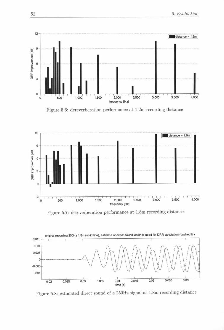
52 5. Evaluation

,'.0003.5003.0002.0J0 2.500

frequency [Hz)1.5001.000500

oo

12_distance. 12mI

m 9

"-•~•> 60~•~~0 3

Figure 5.6: dereverberation performance at 1.2m recording distance

12

,to

"-• 6~•>.~3~~0

0

" 0 500 1.000 1.500 2.000 2.500ffeq.,Jency 1Hz]

3.000 3500 '.000

Figure 5.7: dereverberation performance at 1.8m recording distance

,,,,,,,,\'

0,015

0,01

OOOS

o.(lOOS

-0,01

original recording 250Hz 1,8'n (so~d line), e$lmale of direa 6OUI'Id which is used lor DAR caltUation (dashed lill

,c,,,,,,,,,,

002 0.025 003 0.035 0.04 0.045lime [s]

005 0.055 005

Figure 5.8: estimated direct sound of a 250Hz signal at 1.8m recording distance

6. Summary

To conclude the work, this chapter is intended to give a brief overview and ratingover what has been found out and where possible "next steps" could lead to.

6.1 ConclusionAt first, the goal of demonstrating a dereverberation method for single sine waveswhich does not rely on any assumptions about the environment, has been achieved.The improvements in the direct-to-reverberant ratio for the various test recordingsarc mostly equal or better than those achieved with beamforming algorithms andmultiple microphones in [Gaubitch05]. However, the restriction to single sine wavesis a strong simplification and so the new approach is far from being applicable in thereal world. \Vhether the proposed method will ever be useful for the dereverberationof real-world signals highly depends on the practicability of the extensions presentedin the chapters 2.3.2 and 2.3.3.

\VhiIe the overall approach looks promising due to the comparably high trackingaccuracy of the PLLs, this accuracy must be incrca:;ed even further. In fig. 5.5 itcan be seen what happens if the measurement of a frequency, for example, is justslightly ""Tong. Additionally, the experience gained throughout this work suggeststhat improvements must also be made in the robustness of both the PLL trackingand the detection scheme which is used to detect the arrival of a wavefront.

Finally, the transition from single sine waves to multiple sine waves will also be adifficult step, but one that is absolutely necessary in order to tell reflections andphoneme-changes apart. To analyze multiple frequency components, the recordedsignal must be splitted using bandpass filters which results in a smoothing of therecorded signal. In a smoothed signal, however, it will be more difficult to detectrapid changes which, in turn, is needed to find out when a reflected ,vavefront arrivesat the microphone.

6.2 Future WorkThe next steps to develop the dcreverberation algorithm further are the implemen-tation of the two methods presented in the chapters 2.3.2 and 2.3.3, in order to

54 6. Summary

find out if and how well the proposed approach can handle signals with multipletime-varying frequencies. The transition from artificial harmonic complexes to realspeech can only be made after the algorithm ,,,arks very well on artificial signals.

A. Matlab Code

A.I PLL Initialization Script

%----------------------------------------------------------------------:l % PLL Parameters3 %-------------------------------------------------------------------- __4 addpath (' .. /Simulink_Hodels');

•G !t define audio file if this script is not run in b<'ltch mode7 if exist('batchJob', 'var'j == 0 II batchJob =- 08 audioFile = [' .. /data/sineRecordings. 48.120cm/'9 'single_frequencies/1000Hz.waV']i10 end

"12 % extract frequencies played in the file out of the filename13 if exist (audioFile, 'file') == 214 [~, filename, ~] = fileparts(audioFile)i"III % parse filename to find PLL center frequencies17 % PLLBase: center frequency ot first PLL18 % PLLSpacing: distance between center frequencies19 ; PLLCount: number of PLLs to use~o if ....•isempty (strfind (audioFile, 'harmonics')~I PLLBase = str2double (filename (l: 3) ) i~2 PLLSpacing = PLLBase;~3 PLLCount = (str2double (filename (5: 8) ) -PLLBase) IPLLSpacing;~4. else~~ pos_Hz •• st rfind (filename, 'Hz' ) ;~(1 PLLBase •• str2double (f ilename (1: pOS_Hz-l) ) ;27 PLLSpacing = 0;~8 PLLCount = 1;

"31 end32 else33 error('File does not exist');34. end

"

% exit if file could not be found

56

30 clear filename;

"38 % gp.neral p3rameters39 i_sample 48000;40 t_sample = l/f_sample;

% sample ~ate [Hz]% sample time [s]

A. MarIah Code

% use bandpass-prefilter yes/no% PLL input bandwidth (= BW of prefilter)% undef. range between pass- and stopband

"41 % calculate center frequencie:,; for all PLLs43 PLLCenter = PLL8ase + (O:PLLCount-l) * PLLSpacing;••4!> % pref i lter parameters46 use-prefilter = 0;47 8_1= 100;48 prefilterSlope 50;

[Hz][Hz]

% locp filter gain% set NCOto fixed trequency yes/no

.,50 % phase detector parameteLs51 hilbertLength = 1200; % length of the phase detector hilbert filter

"&3 % loop filter parametersM zeta = sqrt (2) /2; % damping factor

"56 % set SNR_i according to measured values57 if ~isempty(strfind(audioFile, 'lDem'))M SNR_i ••46.4;w elseif ....•isempty (strfind (audioFile, '60cm'))60 SN~i = 34.3;61 elseif ....•isempty(strfind(audioFile, '120cm'»)(I'J SNR_i = 29.1;63 elseif ....•isempty(strfind(audioFile, '180cm'))l,I4 SNR_i = 21.5;6& end~67 % veo parameters68 kappa - 1;69 lock_nco 0= 0;mn '1;;- - ---- - --- - ---- - --- - - ---- ---- ----- ----- ---- ---- - ---- ----- ---- - --- - ----

n % Loading PLL Input Signal73 %-------- -------------------------------------------------------------

"75 disp('Loading input audio file');

"77 % fiI'st check if the file exists at <11178 if exist taudioFile, 'file') =0= 279 [pathname, filename, ext) 0= fileparts (audioFile);~81 % replace path with'.' if it is err.pty (current. folder)8J if strcmp (pathname, , ') =•• 183 pathname = .';

84 end

"~ , check if the file is a .wav file87 if strcmp(ext,' .wav') 0== 188 % convert .wav to .mat if no corresponding ,mat exists89 if exist (streat (pathname, filesep, filename, , .mat'), 'file ') ,.. 290 wavToMat(f_sample, audioF ile) ;

end" 'l; cr.ange file name to the same file U[;i;lg .:nat as ending

audioFile = strcat (pathname, filesep, filename, ' .mat');

A.i. PLL Initialization Script 57

95 end~97 % finally load the file98 load(strcat (pathname, filesep, filename,' .mat'));gg else100 error('File does not exist'); % exit if file could not be found101 end'"103 % reverse VQctor if needed for backwards processing:104 if exist('reverseProc', 'var') == 1 && reverseProc -'" 1105 wavesignal(:,2) = wavesignal(end:-l:l,2);lOll end

'"l~ % create empty vector for filtered versions of the original signal100 ws_append = zeros(length(wavesignal(:,l),PLLCount);llO wavesignal - horzcat (wavesignal,ws_append);

'"112 % copy unfiltered version of input to each channel113 for i = I:PLLCount114 wavesignal (:,i+2) '"wavesignal (:,2);116 end

'"117 clear pathname filename ext ws_append;

'"119 %------------------------------------------------------------------- _120 % Calculating Prefilter Coefficients121 %--------------------------------------------- _'"123 if use-prefilter == 1

'"121> diSp('Applying bandpass filteL'bank');

'" 'Filter lengths:';str'"'"1::9 for i = I :PLLCount,~'"'"'",,.

% calculate passbandfpl PLLCenter(i)fp2 = PLLCenter(i) +

edgesB_i I 2;8_i I 2;

'"'"'"'"'"'",.,'"

% calculate stopband edgesfstl fpl - prefilterSlope;fst2 = fp2 + prefilterSlope;

i design filterd - fdesign.bandpass('?stl,Fpl,Fp2,Fst2,Astl,Ap,Ast2',

fstl,fpl,fp2,fst2,60,I,60,f_sample);hd = design (d, 'cheby2' , 'matchexact ly' , 'passband' );

,..,.,'"'"'"'"'"'"'"'"

% zero-phase filter the data: filter forward, reverse in time% filter backward and rever::;€in time againwavesignal(:,i+2) ~ filter(hd,wavesignal(:,2);wavesignal(:,i+2) wavesignal(end:-l:l,i+2);wavesignal (:,i +2) filter (hd,wavesignal (:,i+2) );wavesignal (:,i+2) wavesigna1 (end:-1: 1,i+2) ;

str = [str ' , num2str(hd.order)j;

clear fstl fst2 fpl fp2 d hd;

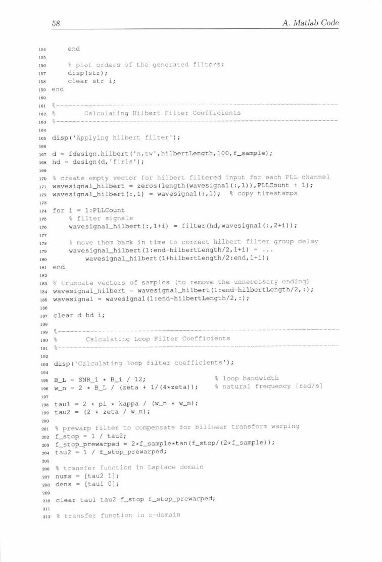
filter(hd,wavesignal(:,2+i)};

58 A. MatJab Code

154 end

'"156 't. P ot orders of the generated fi.~tcrs:157 disp(str);158 clear stl' i;159 end

'"161 %---------------------------- --------------------------------- ---162 % Calculating Hilbert Filter Coefficients163 %----------------------------------------------------------------------'"165 disp('Applying hilbert filt€:r');

'"161 d '= fdesign. hilbert (' n, tw', hilbertLength, 100, f_sample);HI6 hd = design (d, 'f irIs');

'"170 % create empty vector for hilbert filtered input for each PLL cl1a:-lnel171 wavesignal_hilbert ~ zeros(length(wdvesignal(:,l)),PLLCount + 1);172 wavesignal_hilbert(:,l) = wavesignal(:,l); % copy timestamps,n174 for i = 1:PLLCountIn; % filter signals176 wavesignal_hilbert (:, 1+i)on178 % move them back in time to correct hilbert filter group delay179 wavesignal_hilbert (1:end-hilbertLength/2, l+i) = •••

180 wavesignal_hilbert (1+hilbertLengthl 2: end, 1+iJ ;181 end..,183 % truncate vectors of samples (to remove the unnecessary ending)18~ wavesignal_hilbert = wavesignal_hilbert (l :end-hilbertLength/2, :);185 wavesignal = wavesignal(1:end-hilbertLength/2, :);..,187 clear d hd i;..,189 %------------------~~--------~--------~--------------------------------190 % Calculating Loop Filter Coefficients191 %~~-----------------~-----------------~--------------------------------'"193 disp ('Calculating loop filter coefficients ');

'"195 B_L •• SNR_i • B i I 12;196 w_n 2. B_L I (zeta + II (4".zeta);

'"

% loop bandwidth% natural frequency [rad/s]

2 • pi • kappa / (w_n ". w_n);(2 • zeta I w_n);

198 tau1199 tau2wo201 % prewarp filter to compensate for bilinear transform warping202 f_stop = 1 I tau2;W3 f_stop-prewarped" 2.f_sample.tan(f_stop/(2*f_sample));~4 tau2 - 1 I f_stop-prewarped;

'"2(16% transfer function in L<lplace dcrr,ain207 nums [tau21);208 dens" [taul 0);

'"210 clear tau1 tau2 f_stop f_stop-prewarped;m211 'i transfer fu"ction in z domain

A.2. Dereverberation Script 59

213 [numz,2H numz216 denz -

denz) - bilinear(nums,dens,f_sample);real (numz);real (denz);

'"217 disp ('+-- -------------- ---------- ,);218 disp (' t Loop Parameters:');219 disp«('1 w_n = " num2str(w_n I (2*pi»), , Hz'»;220 disp ([' I zeta '"'" num2str (zeta) 1);221 disp(['1 ~_f""'po " num2str(1.8*w_n*(zeta+l)1 (2"pi)), Hz'J);222 disp (('I .:._f_L " num2str (2"zeta*w_n I (2"pi), Hz' I);223 disp(['1 T_L = " num2str(l000" 2"pi/w_n), 'ms');224 disp ((' I B_L = " num2str (B_L), , Hz' 1);226 disp ('t--------------------------');,~227 clear nums dens zeta f_lock w_n B_i B_L SNR_l;

'"229 %------------------------------------~~--------------------------------:l3O % Load model and set simulation duration231 % ---- --- ------ -------- --------- ------ ---- ------- --- ---- ----------------

'"233 if exist('batchJob', 'var') == 0 II batchJob =•• 02~ disp('Loading Simulink model');235 load_system (•..i Simul ink_Models IPLL_Hilbert '1;2~ open_system(' ../Simulink_Models/PLL_Hilbert');237 end

'"239 % set durat ion of simulat ion240 set-param ('PLL_Hilbert', •StopTime', num2str (wavesignal (end, 1),15) );

A.2 Dereverberation Script

f_sample = 48000;,3 amplFolder = 'sine_funlocked/single_frequencies.120cm/';4 phaseFolder = 'sine_flocked/single_frequencies.120c~/';,(I freg = 1000;,8 axes List - (1; % list for axes to bp. synchronized afterwards,10 %% '*~*'*'#'****'f*j'i4f,i#***i*#Jj.****'~;"";"""f.#",*.J,., •••"11 % load and smooth phase and amplitude

"13 % load both files14 fileName" strcat(num2str(freq), 'Hz.out.mat');I~ amplObj = ProcessedSineRecording (strcat (amplFolder, fileName») i

1(1 phaseObj - ProcessedSineRecording(strcat(phaseFolder,fileName));"18 % load amplitude and pha.se19 a = amplObj.getSignalBylndex(4);20 pll amplObj.getSignalBylndex(l);21 pH pll (:,2) ;22 mic - phaseObj.getSignalBylndex(l);23 mic - mic (:,1) i

24 P phaseObj.getSignalBylndex(2);2~ f = amplObj.getSignalBylndex(3);"

60 A. Matlab Code

O:length(a_s)-l;times .1 f_sample;

~7 t move amplitude forwards in time due to the backwards processinq28 a(601:end) = a(l:enct-600);29 f(601:end) = f(l:end-600);30 pll (601 :end) = pH (1 :enct-600);31 '.1(1:600) = 0;32 f(1:600) = 0;33 pll(1:600) =0;

"3~ % smooth amplitude and phase by a median filter36 p_s medfiltl (p, 48);37 d_S medfiltl (a, 48);38 f_s medfiltl(f,48);

"40 clear a p f out;

"42 %% 'ft~'t~*;j.;*""**ftt*'t.*#t*t,,;tt"tt~'t#tf*#*"*"#"'R"*'~;#tt43 % determine start and end of direct sound

"4~ % find maximum and ninimum of derivative of tee microphone signal48 % (add 600 to corr~ensate for backwards processing)47 startSample - amplObj.getStartSample() + 600;48 stopSample = amplObj.getStopSample() + 600;

50 disp( ['start of direct sound at ' num2str(freq) 'Hz at sample~I num2str (startSamplell);~2 disp(['end of direct sound at ' num2str(freq) 'Hz at sample'1\3 num2str (stopSample) l);

••1111 clear peaks peakTimes maxlndex diffA d hd;

"117 %% .~'***;t.##t.#,#.t,#;i"*#*~#*ftt';t"'.tf".f"*f";ft'f"t,.,;,t"1\5 % initialize vectors for calculated reverb amplitude and phase

"60 times61 times

"63 a_ref - zeros(length(a_s),l);64 f_ref zeros(length(a_s),l);611 p_ref zeros(length(a_sl,l);66 a_ref (startSamp1e: stopSamplel median (a_s (startSamp1e:67 startSamp1e+48) 1;68 f_ref(startSample:stopSample) trimrnean (f_s (startSample: ...69 stopSample), 10);70 p_ref(startSamp1e:stopSamp1e) ~ mod(median (p_s (startSample:71 startSamp1e+48), 2*pi);

"73 %% ""f't','f""tt"""""'#"#'t"'k"'#*"""""#f""'t",.,;,74 % create reference signal to measure the DRR

"76 % cut beginning of direct sound out of the microphone signal77 searchFrame = smooth (mic(startSample-48:startSample+96) ,5);

"79 % ger.eratp. one period of the ~eferenC0 sine 'Naveso tref "" 0:1/48000:1/freq;81 ref Frame = a_ref (startSample) * sin (2*pi*f_ref (startSample) *tref);

"'83 % calculate time of aIrival by finding t~e correlation peak84 ( ....•, corrpeakl = max(xcorr(refFrame, searchFramel);

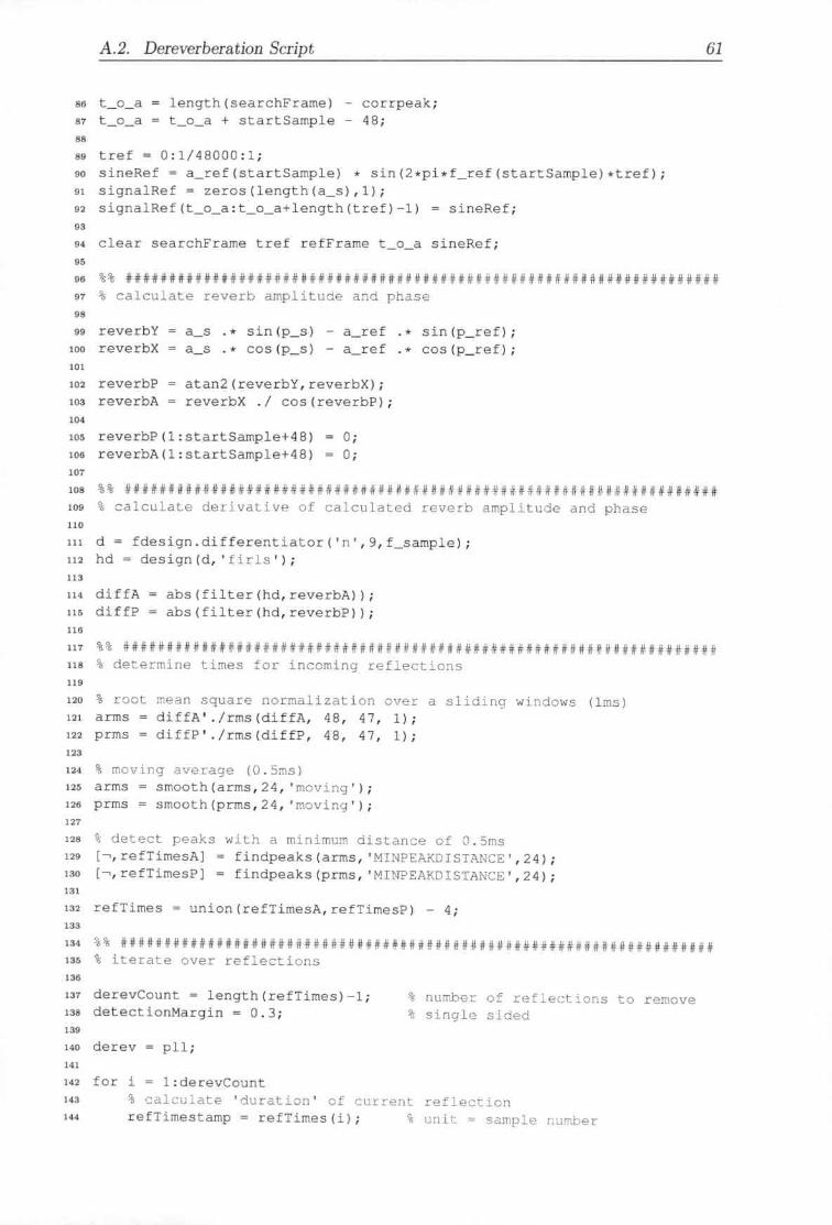
A.2. Derevcrbcrlltion Script 61

atan2(reverbY,reverbX)ireverbX ./ cos(reverbP);

~ t_o_a - length (searchFrame) - corrpeak;87 t_o_a = t_o_a + startSample - 48;""89 tref = 0:1/48000:1;00 sineRef = a_ref(startSample) • sin(2*pi.f_ref(startSample).tref);91 signalRef = zeros(length(a_s),l);92 signalRef It_o_a:t_o_a+length (tref)-ll - sineRef;"94 clear searchFrame tref refFrame t_o_a sineRef;"ge %% t;i','*"i'tfi'*'*,~*',',j,tt"",*",t'*"'#""t"""""f,*" ••,97 % calculate reverb amplitude and phase"99 reverbY a_s.* sin(p_s) - a_ref .• sin(p_ref);100 reverbX = a_s .* cos (p_s) - a_ref .• cos(p_ref);."102 reverbP103 reverbA".105 reverbP (1:startSample+48) 0;loe reverbA(l:startSample+48) 0;."I~ %% *'j""""t"f_i""""f'.~"j'f""""'_k'#I'#""#1""""1'1'109 % calculate derivative of calculated reverb amplitude and phase",111 d'" fdesign.differentiator('n',9,f_sample);112 hd = design (d,'firls');."114 diffA115 diffP

abs(filter(hd,reverbA));abs(filter(hd,reverbP));

\ nu~ber of reflections to remove\ single s,ided

".U7 %% t"f"*"I"#'f".;llk"*'~'t#k""t""#,"*'II't"j'""".,*"'"118 -% determine times for incoming reflections'"l~ % root mean square normalization over a sliding ~indows (lms)12I arms = diffA'./rms(diffA, 48, 47, 1);122 prms = diffP' ./rms (diffP, 48, 47, 1) i

'"124 % moving aVel"age (O.5ms)121> arms - smooth (arms,24, 'moving');12fI prms = smooth(prms,24,'moving');."128 % detect peaks with a minimw.::'1distance of O.5ms129 [ ....•, refTimesA) - findpeaks (arms, 'MINPEAKDISTANCE', 24);130 ( ....•,refTimesP] "" findpeaks(prms, 'MINPEAKDISTANCE',24)i'"132 refTimes ""union(refTimesA,refTimesP) - 4;'"1M %% ""f""t."""*",**, ••".,t¥.,.",*"",,*,,,.ti**"'*'*'1".,*,131> \ iterate over reflections."131 derevCount ..,length (refTimes) -1;138 detectionMargin - 0.3;'"140 derev = pll;'"142 for i '"'1 :derevCount1~3 % calculate 'duration' of current reflection144 refTimestamp = refTimes (i); % unit ;0;0 sa.mple nurrJ:,er

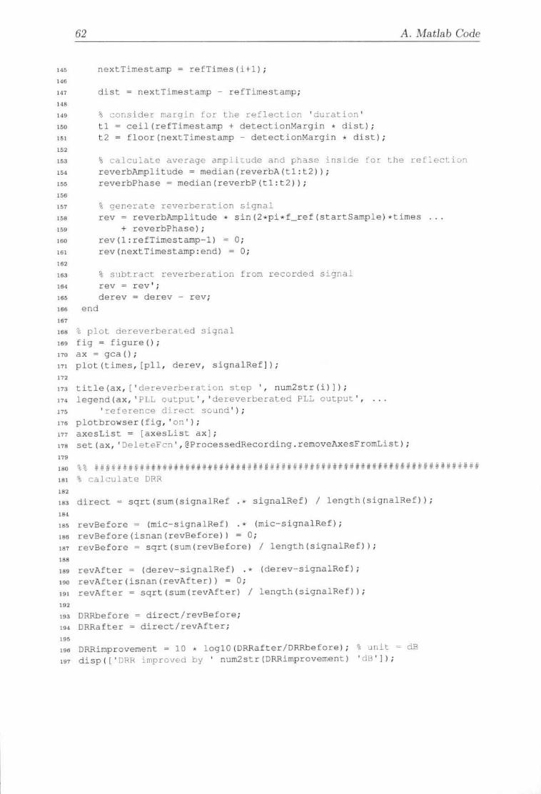
62 A. Matlab Code

146 next Timestamp = ref Times (i"'I);

'"147 dist = nextTirnestamp - ref Timestamp;

'"149 % consider margin for the reflection 'cl,;ration'160 tl ceil (ref Timestamp + detectionMargin .• dist) i

161 t2 = floor (nextTimestamp - detectionMargin •. dist);

'"163 % calculate average amplitude and phase inside for the ref:.E!clion154 reverbAmplitude = median(reverbA(tl:t2));165 reverbPhase '"' median(reverbP(tl:t2));

'"157 % generate reverberation signal158 rev = reverbAmplitude .•. sin (2•.pi*f_ref (startSample) •.times159 + reverbPhaseJ;160 rev(l :refTimestamp-l) OJ161 rev(nextTimestamp:end) : 0;

'"HI3 % subtract reverberation from recorded signal164 rev = rev';16.'> de rev = de rev - rev;166 end

'"1611 % plot dereverberated signal1119 fig = figure () ;170 ax '"' gca () ;171 plot (times, [pll, dere'l, signaIRefl);

'"173 title (ax, ['dereverberation step', num2str (i) J);174 legend (ax, 'PLL output.', 'dere'ler:herated PLL output',In 'reference direct- sound');176 plotbrowser (fig, 'on' ) ;177 axesList = [axesList ax];17/1 set (ax, 'DeleteFcn', @ProcessedRecording.removeAxesFromList);

'"IKO %l ,~t~H#,*H#*'~~*t,••~,*f,~jt'H~8*j'.i'*'fi.i,••***fJ*~ff'j,i"""'"1/11 % calculate DRR

'"1/13 direct - sqrt(sum(signalRef .* signalRef) / length(signaIRef»);

'"1/1.'> revBefore ~ (mic-signalRef) * (mic-signaIRef);1811 re'lBefore (isnan (re'lBefore)) = 0;187 re'lBefore ~ sqrt (sum(rev8efore) / length (signalRef));

'"189 revAfter •• (derev-signalRef) . * (dere'l-signalRef);19<1 re'lAfter(isnan(revAfter») •• 0;191 re'lAfter •• sqrt(sum(re'lAfter) / length(signalRef);

'"193 DRRbefore = direct/re'lBefore;194 DRRafter = direct/revAfteri

'"1911 DRRimprovement •• 10 * 10g10 (DRRafter/DRRbefore) i % unit = dB197 disp ([' DI1Rimproved by , num2str (DRRimpro'lement) , dH' I ) ;

Bibliography

[13est93J Roland 13est. Phase-locked loops: theory, design and ap-plications. 2nd ed. New York: ~IcGraw-Hill, 1993. ISBN:ll-07-911386-9.

[DINI311-I] DIN German Institute for Standardization: FundamentalTechnical Standards Committee. DIN 1311-1: (Mechani-cal) vibrations, oscillation and vibration systems - Part 1:Basic concepts, survey. Beuth Verlag GmbH, Feb. 2000.

fEstienncOl] Claudio Estienne, Patricia Pelle, and Juan Pablo Pi-antanida. "A Front-end for Speech Recognition SystemsUsing Phase-Locked Loops". In: Proceedings of the Work.shop in Infonnation Processing and Control (RPIC).Santa Fe, 2001, pp. 88-91.

[Gardner05] Floyd M. Gardner. Phaselock techniques. 3rd ed. Hoho-ken, New Jersey: \Viley-Intersciencc, 2005. ISDN: 978-Q..471-43063-6.

[Gaubitch05] NikoIay Gaubitch nnd Patrick Naylor. "Analysis of thedereverberation performance of microphone arrays". In:Proceedings of the International Workshop on AcousticEcho and Noise Control (IlVAENC). Eindhoven, 2005.

IKarimi-GhartemaniOl} ~-1a.'loud Karimi-Ghartemani and ~,1. Reza Iravani. l'Anew phase-locked loop (PLL) system". In: Proceedings ofthe IEEE Midwest Symposium on Circuits and Systems(MIVSCAS). Vol. 1. Dayton, Ohio, 2001, pp. 421-424.001:10.1109 /MWSCAS.2001.986202.

[Kinoshita05a) Keisuke Kinoshita, Tomohiro Nakatani, and MasatoMiyoshi. l'Efficient Blind Dereverberation Framework forAutomatic Speech Recognition". In: Proceedings of the Eu-ropean Conference on Speech Communication and Tech-nology (INTERSPEECH). 2005, pp. 3145-3148.

[Kinoshita05b] Keisuke Kinoshita, Tomohiro Nakatani, and Masato~Hyoshi."Fast Estimation of a Precise DereverberationFilter based on Speech Harmonicity". In: Proceedings ofthe IEEE International Conference on Acoustics, Speechand Signal Processing (ICASSP). Vol. 1. 2005, pp. 1073-1076.001: 1O.1109/ICASSP.2005.1415303.

64

[McAulay86J

[N akatani03a]

[Nakatani03b]

[Nakatani07)

[Pearson96]

[PoI46]

[Sengpiel1lj

[Smith07]

[Stephens02]

Bibliography

Robert 1JcAuiay and Thomas Quatieri. "Speech analy-sis/Synthesis based on a sinusoidal representation". In:IEEE Transactions on Acoustics, Speech and Signal Pro-cessing 34.4 (1986), pp. 744-754. ISSN: 0096-3518. DOr:

10.1109 /TASSP.1986.116491 O.

Tomohiro Kakatani and t..1asato :Miyoshi. "Blind derever-beration of single channel speech signal based on har-monic structure". In: Proceedings of the IEEE Interna-tional Conference on Acou.stics, Speech and Signal Pro-cessing (lCASSP). Vol. 1. 2003, pp. 92-95. DOl: 10.1109/ICASSP.2003.1198724.

Tomohiro Nakatani, Masato 1-liyoshi, and Keisuke Ki-noshita. "Implementation and effects of single chan-Hel dereverberation based on the harmonic structure ofspeech". In: Proceedings of the International Workshop onAcoustic Echo and Noise Control (lWAENC). Hong Kong,2003, pp. 91-94.

Tomohiro Nakatani, Keisuke Kinoshita, and i\lasato~'fiyoshi."Harmonicity Based Blind Derevcrberation forSingle-Channel Speech Signals". In: IEEE Tmnsactions onAudio, Speech and Language Processing 15.1 (2007), pp. 80-95. ISSN: 1558-7916. DOl: 1O.1I09/TASL.2oo6.872620.

Qiguan Lin et al. "Robust distant-talking speech recog-nit ion". In: Proceedings of the IEEE International Con-ference on Acoustics, Speech and Signal Processing(ICASSP). Vol. 1. May 1996, pp. 21-24. DOl: 10.1109/ICASSP.1996.540280.

Balth. van der Pol. "The Fundamental Principles of Fre-quency Modulation". In: Journal of the Institution of Elec-trical Engineers - Parl III: Radio and Communication En-gineering 93.23 (May 1946), pp. 153-158.

Eberhard Sengpiel, Berlin University of the Arts. Soundpressure p and the inverse distance law l/T. 2011. URL:http:j j www.sengpielaudio.com/calculator- distancelaw .htm (visited on 01/24/2011).

Julius O. Smith. Introduction to Digital Filters with Au-dio Applications. online book. 2007. URL: https:jjccrma.stanford .edu / -jos / fp/ Zero_Phase_Filters_Even_Impulse.html (visited on 01/25/2011).

Donald R. Stephens. Phase locked loops for wireless com-munications: digital, analog and optiml implementations.2nd 00. Boston: Kluwer Academic Publishers, 2002. ISBN:().7923-7602- I.