iTesla’–Enabling’Resiliency’for’Future’Power’Grids ... ·...

iTesla – Enabling Resiliency for Future Power Grids Presenta:on Focusing on WP3 Results

Prof.Dr.-‐Ing. Luigi Vanfre2, Te5ana Bogodorova

Workshop on Resiliency for Power Networks of the Future May 8th 2015, Stockholm, Sweden

Associate Professor, Docent E-‐mail: [email protected]

Web: hDp://www.vanfre2.com

KTH Royal Ins5tute of Technology Stockholm, Sweden

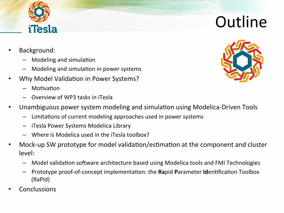
Outline •  Background:

–  Modeling and simula5on –  Modeling and simula5on in power systems

•  Why Model Valida5on in Power Systems? –  Mo5va5on –  Overview of WP3 tasks in iTesla

•  Unambiguous power system modeling and simula5on using Modelica-‐Driven Tools –  Limita5ons of current modeling approaches used in power systems –  iTesla Power Systems Modelica Library –  Where is Modelica used in the iTesla toolbox?

•  Mock-‐up SW prototype for model valida5on/es5ma5on at the component and cluster level:

–  Model valida5on soTware architecture based using Modelica tools and FMI Technologies –  Prototype proof-‐of-‐concept implementa5on: the Rapid Parameter Iden5fica5on Toolbox

(RaPId)

•  Conclussions

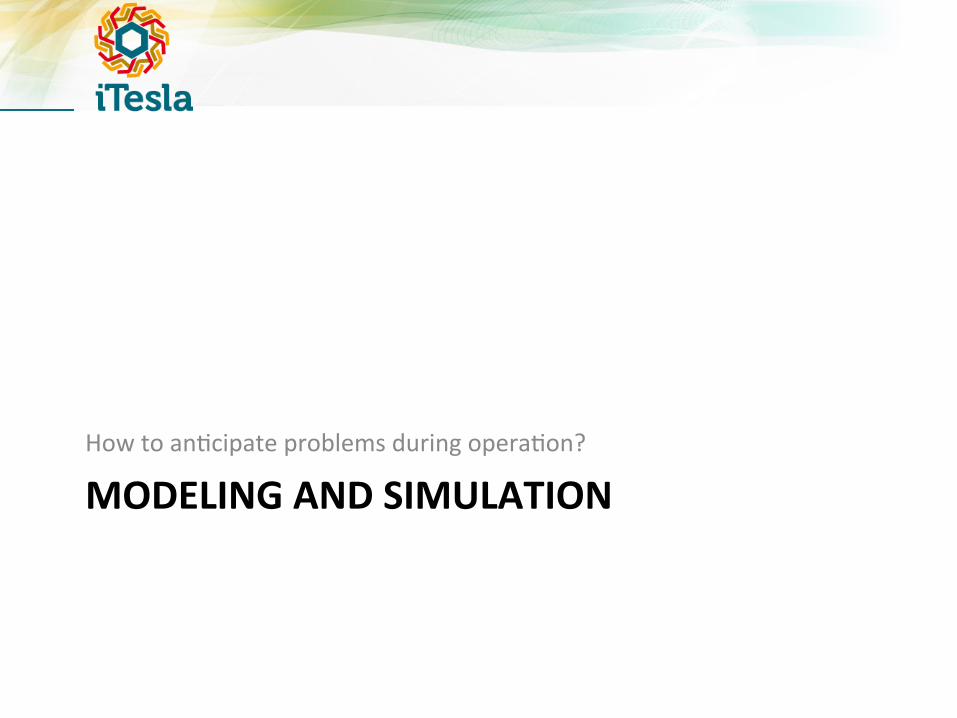
MODELING AND SIMULATION How to an5cipate problems during opera5on?

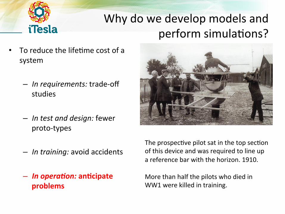
Why do we develop models and perform simula5ons?

•  To reduce the life5me cost of a system

–  In requirements: trade-‐off studies

–  In test and design: fewer proto-‐types

–  In training: avoid accidents

–  In opera)on: an:cipate problems

The prospec5ve pilot sat in the top sec5on of this device and was required to line up a reference bar with the horizon. 1910. More than half the pilots who died in WW1 were killed in training.

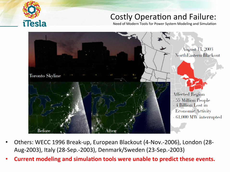
•  Others: WECC 1996 Break-‐up, European Blackout (4-‐Nov.-‐2006), London (28-‐Aug-‐2003), Italy (28-‐Sep.-‐2003), Denmark/Sweden (23-‐Sep.-‐2003)

•  Current modeling and simula:on tools were unable to predict these events.

Costly Opera5on and Failure: Need of Modern Tools for Power System Modeling and Simula5on

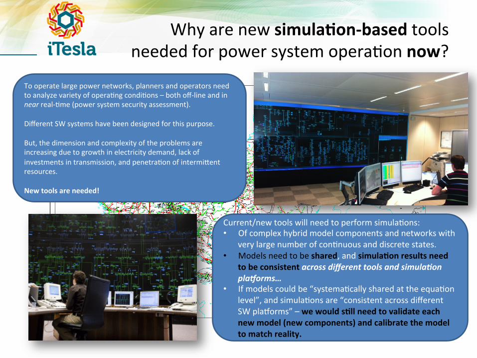
Why are new simula:on-‐based tools needed for power system opera5on now?

To operate large power networks, planners and operators need to analyze variety of opera5ng condi5ons – both off-‐line and in near real-‐5me (power system security assessment). Different SW systems have been designed for this purpose. But, the dimension and complexity of the problems are increasing due to growth in electricity demand, lack of investments in transmission, and penetra5on of intermiDent resources. New tools are needed!

Current/new tools will need to perform simula5ons: •  Of complex hybrid model components and networks with

very large number of con5nuous and discrete states. •  Models need to be shared, and simula:on results need

to be consistent across different tools and simula)on pla4orms…

•  If models could be “systema5cally shared at the equa5on level”, and simula5ons are “consistent across different SW plaiorms” – we would s:ll need to validate each new model (new components) and calibrate the model to match reality.

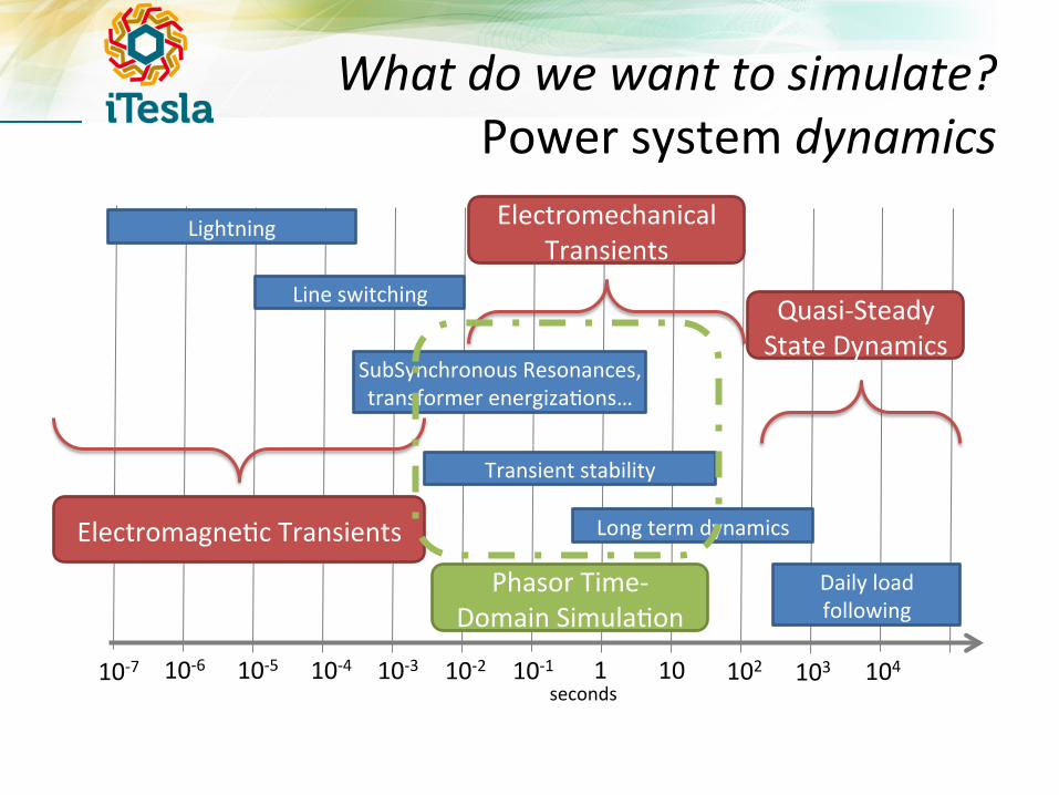
What do we want to simulate? Power system dynamics

10-‐7 10-‐6 10-‐5 10-‐4 10-‐3 10-‐2 10-‐1 1 10 102 103 104

Lightning

Line switching

SubSynchronous Resonances, transformer energiza5ons…

Transient stability

Long term dynamics

Daily load following

seconds

Electromechanical Transients

Electromagne5c Transients

Quasi-‐Steady State Dynamics

Phasor Time-‐Domain Simula5on

Example of Power System Dynamics in Europe February 19th 2011

49.85

49.9

49.95

50

50.05

50.1

50.15

08:08:00 08:08:10 08:08:20 08:08:30 08:08:40 08:08:50 08:09:00 08:09:10 08:09:20 08:09:30 08:09:40 08:09:50 08:10:00

f [H

z]

20110219_0755-0825

Freq. Mettlen Freq. Brindisi Freq. Wien Freq. Kassoe

Synchornized Phasor Measurement Data

Power Systems Status Quo of Modeling and Simula5on Tools

10-‐7 10-‐6 10-‐5 10-‐4 10-‐3 10-‐2 10-‐1 1 10 102 103 104

Lightning

Line switching

SubSynchronous Resonances, transformer energiza5ons…

Transient stability

Long term dynamics

Daily load following

seconds

Phasor Time-‐Domain Simula5on

PSS/E Status Quo: Mul5ple simula5on tools, with their own interpreta5on of different model features and data “format”. Implica@ons of the Status Quo: -‐  Dynamic models can rarely be shared in a

straigh4orward manner without loss of informa)on on power system dynamics (parameter not equal to equa)ons, block diagrams not equal to equa)ons)!

-‐  Simula)ons are inconsistent without dras)c and specialized human interven)on.

Beyond general descrip:ons and parameter values, a common and unified modeling language would require a formal mathema5cal descrip5on of the models – but this is not the prac5ce to date.

These are key drawbacks of today’s tools for tackling pan-‐European problems.

Common Architecture of « most » Available Power System Security Assessment Tools

Online

Data acquisi:on and storage

Merging module

Con:ngency screening (sta:c power flow)

Synthesis of recommenda:ons for the operator

External data (forecasts and snapshots)

“Sta5c power flow model”

That means no (dynamic) :me-‐domain simula5on is performed.

The idea is to predict the future behavior under a given ‘con5ngency’ or set of con5ngencies.

BUT, the model has no dynamics – only nonlinear algebraic equa5ons.

Computa5ons made on the power system model are based on a “power flow” formula5on.

Result : difficult to predict the impact of a con5ngency without considering system dynamics!

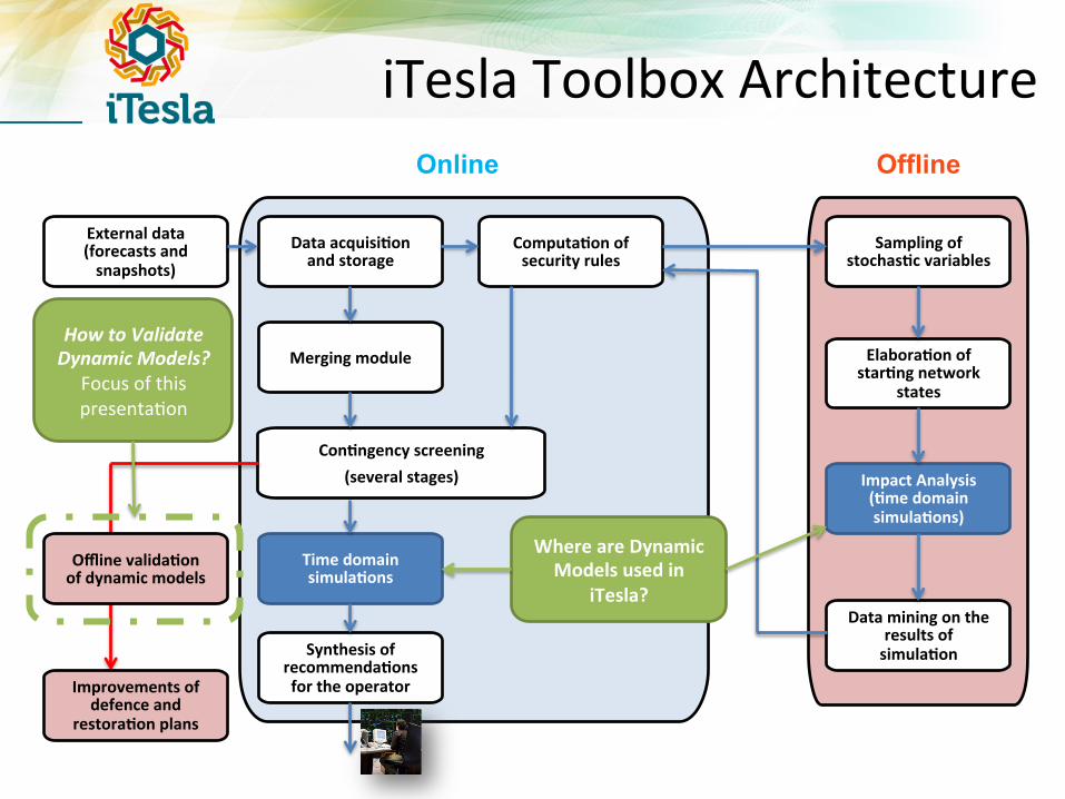
iTesla Toolbox Architecture

How to Validate Dynamic Models?

Focus of this presenta5on

Online Offline

Sampling of stochas:c variables

Elabora:on of star:ng network

states

Impact Analysis (:me domain simula:ons)

Data mining on the results of simula:on


Merging module

Con:ngency screening (several stages)

Time domain simula:ons

Computa:on of security rules



Improvements of defence and

restora:on plans

Offline valida:on of dynamic models

Where are Dynamic Models used in

iTesla?

WHY POWER SYSTEM MODEL VALIDATION?

Mo5va5on

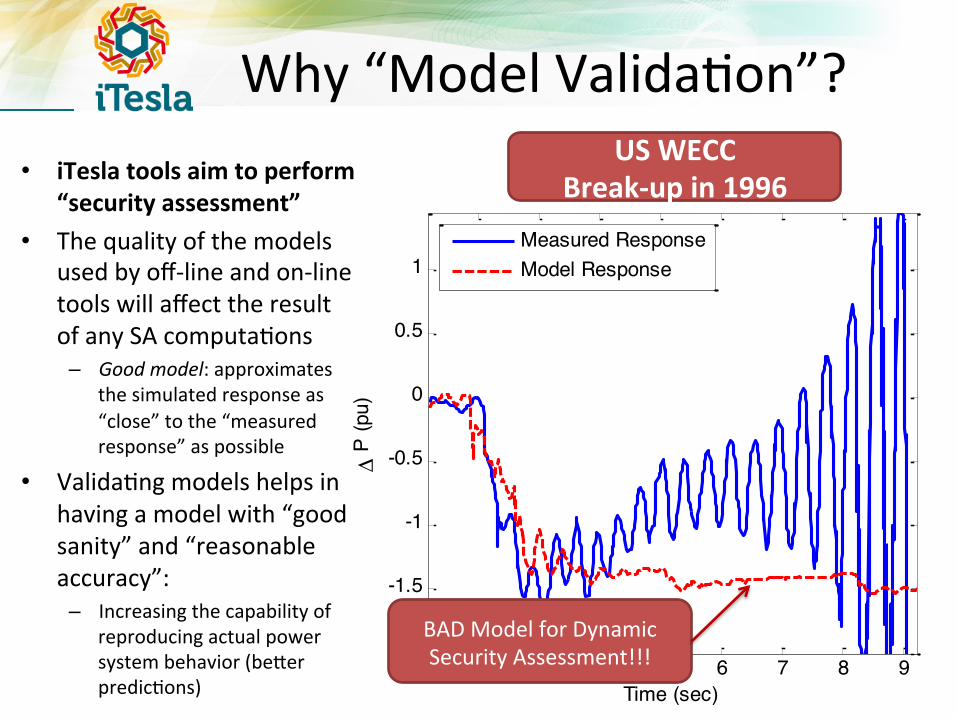
Why “Model Valida5on”? •  iTesla tools aim to perform

“security assessment” •  The quality of the models

used by off-‐line and on-‐line tools will affect the result of any SA computa5ons

–  Good model: approximates the simulated response as “close” to the “measured response” as possible

•  Valida5ng models helps in having a model with “good sanity” and “reasonable accuracy”:

–  Increasing the capability of reproducing actual power system behavior (beDer predic5ons)

2 3 4 5 6 7 8 9-2

-1.5

-1

-0.5

0

0.5

1

Δ P

(pu)

Time (sec)

Measured ResponseModel Response

US WECC Break-‐up in 1996

BAD Model for Dynamic Security Assessment!!!

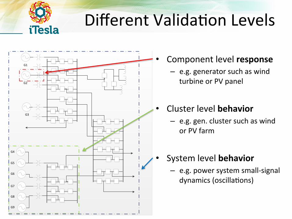
Different Valida5on Levels

•  Component level response –  e.g. generator such as wind

turbine or PV panel

•  Cluster level behavior –  e.g. gen. cluster such as wind

or PV farm

•  System level behavior –  e.g. power system small-‐signal

dynamics (oscilla5ons)

G1

G2

G3

G4

G5

G7

G6

G8

G9

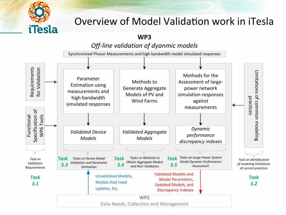
Overview of Model Valida5on work in iTesla

Parameter Estimation using

measurements and high bandwidth

simulated responses

Validated Device Models

Methods for the Assessment of large-‐

power network simulation responses

against measurements

Methods to Generate Aggregate Models of PV and

Wind Farms

Validated Aggregate Models

Tasks on Device Model Validation and Parameter

Estimation

Tasks on Methods to Obtain Aggregate Models

and their Validation

Tasks on Large-‐Power System Model Dynamic Performance

Assessment

WP3Off-‐line validation of dyanmic models

Dynamic performance

discrepancy indexes

Synchronized Phasor Measurements and high bandwidth model simulated responses

Requ

iremen

ts

for V

alidation Lim

itations of common m

odeling practices

Task on Validation

Requirements

Task on Identification of modeling limitations of current practices

Validated Models and Model Parameters,

Updated Models, and Discrepancy Indexes

Unvalidated Models, Models that need updates, Etc.

WP2Data Needs, Collection and Management

Functio

nal

Specificatio

n of

WP6

Too

ls

Task 3.1

Task 3.2

Task 3.3

Task 3.4

Task 3.5

UNAMBIGUOUS POWER SYSTEM MODELING AND SIMULATION USING MODELICA-‐DRIVEN TOOLS

Modeling and Simula5on

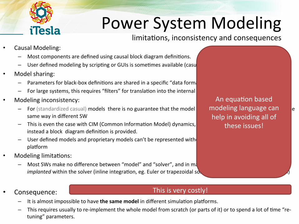
Power System Modeling limita5ons, inconsistency and consequences

•  Causal Modeling: –  Most components are defined using causal block diagram defini5ons. –  User defined modeling by scrip5ng or GUIs is some5mes available (casual)

•  Model sharing: –  Parameters for black-‐box defini5ons are shared in a specific “data format” –  For large systems, this requires “filters” for transla5on into the internal data format of each program

•  Modeling inconsistency: –  For (standardized casual) models there is no guarantee that the model defini5on is implemented “exactly” in the

same way in different SW –  This is even the case with CIM (Common Informa5on Model) dynamics, where no formal equa5ons are defined,

instead a block diagram defini5on is provided. –  User defined models and proprietary models can’t be represented without complete re-‐implementa5on in each

plaiorm •  Modeling limita5ons:

–  Most SWs make no difference between “model” and “solver”, and in many cases the model is somehow implanted within the solver (inline integra5on, eg. Euler or trapezoidal solu5on in transient stability simula5on)

•  Consequence: –  It is almost impossible to have the same model in different simula5on plaiorms. –  This requires usually to re-‐implement the whole model from scratch (or parts of it) or to spend a lot of 5me “re-‐

tuning” parameters.

This is very costly!

An equa5on based modeling language can help in avoiding all of

these issues!

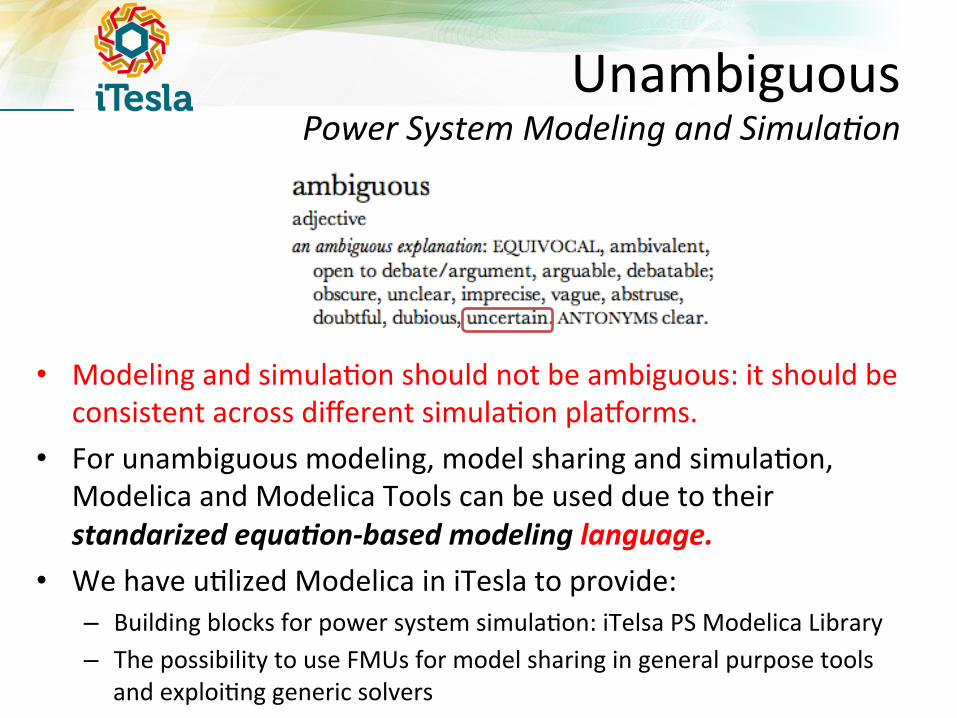
•  Modeling and simula5on should not be ambiguous: it should be consistent across different simula5on plaiorms.

•  For unambiguous modeling, model sharing and simula5on, Modelica and Modelica Tools can be used due to their standarized equa)on-‐based modeling language.

•  We have u5lized Modelica in iTesla to provide: –  Building blocks for power system simula5on: iTelsa PS Modelica Library –  The possibility to use FMUs for model sharing in general purpose tools

and exploi5ng generic solvers

Unambiguous Power System Modeling and Simula@on

iTesla Power Systems Modelica Library

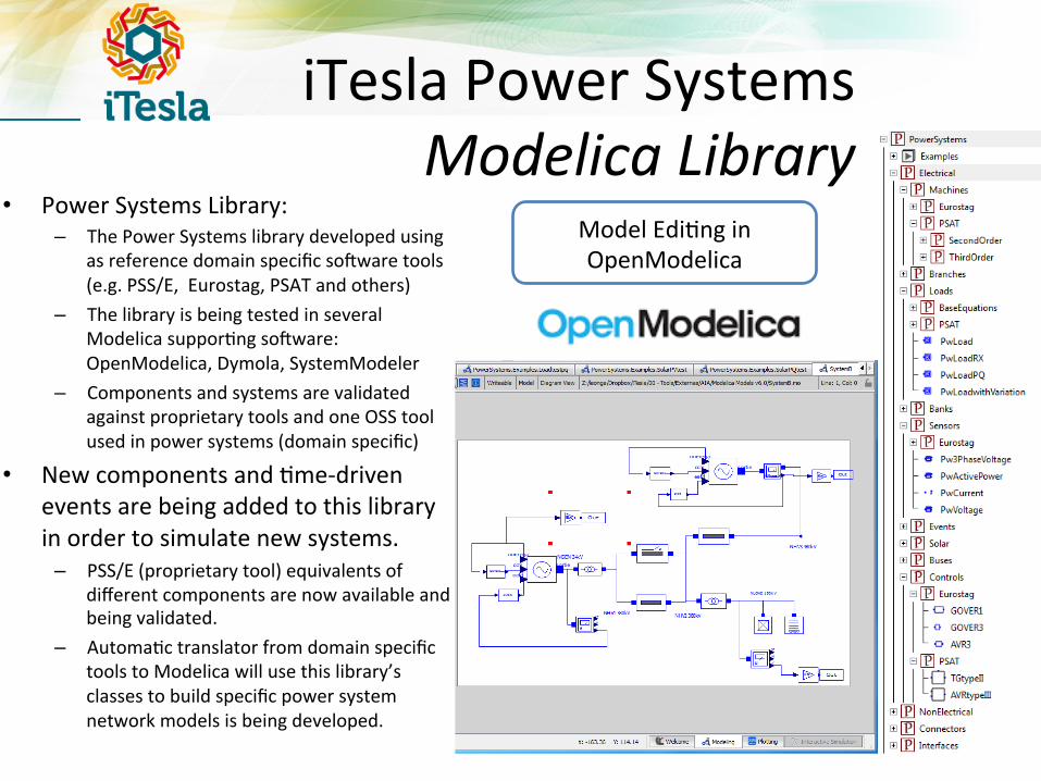
•  Power Systems Library: –  The Power Systems library developed using

as reference domain specific soTware tools (e.g. PSS/E, Eurostag, PSAT and others)

–  The library is being tested in several Modelica suppor5ng soTware: OpenModelica, Dymola, SystemModeler

–  Components and systems are validated against proprietary tools and one OSS tool used in power systems (domain specific)

•  New components and 5me-‐driven events are being added to this library in order to simulate new systems.

–  PSS/E (proprietary tool) equivalents of different components are now available and being validated.

–  Automa5c translator from domain specific tools to Modelica will use this library’s classes to build specific power system network models is being developed.

Model Edi5ng in OpenModelica

Model Edi5ng in Dymola

SW-‐to-‐SW Valida5on of Models in Domain Specific Tools used by TSOs

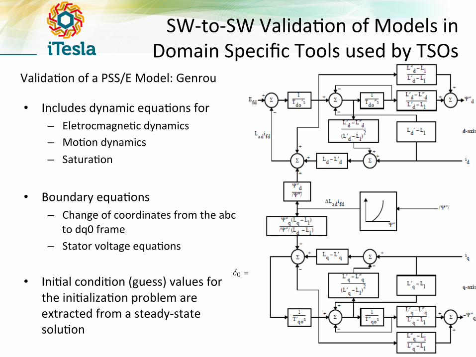
•  Includes dynamic equa5ons for –  Eletrocmagne5c dynamics –  Mo5on dynamics –  Satura5on

•  Boundary equa5ons –  Change of coordinates from the abc

to dq0 frame –  Stator voltage equa5ons

•  Ini5al condi5on (guess) values for the ini5aliza5on problem are extracted from a steady-‐state solu5on

Valida5on of a PSS/E Model: Genrou

Typical SW-‐to-‐SW Valida5on Tests Modelica vs. PSS/E

•  Basic Test Network

•  Perturba5on scenarios

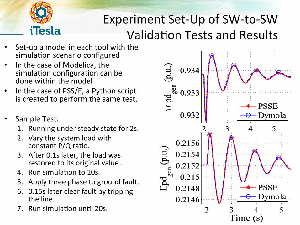
•  Set-‐up a model in each tool with the simula5on scenario configured

•  In the case of Modelica, the simula5on configura5on can be done within the model

•  In the case of PSS/E, a Python script is created to perform the same test.

•  Sample Test: 1.  Running under steady state for 2s. 2.  Vary the system load with

constant P/Q ra5o. 3.  ATer 0.1s later, the load was

restored to its original value . 4.  Run simula5on to 10s. 5.  Apply three phase to ground fault. 6.  0.15s later clear fault by tripping

the line. 7.  Run simula5on un5l 20s.

Experiment Set-‐Up of SW-‐to-‐SW Valida5on Tests and Results

Modelica

PSS/E

Python

SW-‐to-‐SW Valida5on of Larger Grid Models

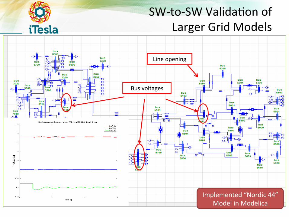
Original “Nordic 44” Model in PSS/E

Line opening

Bus voltages

Implemented “Nordic 44” Model in Modelica

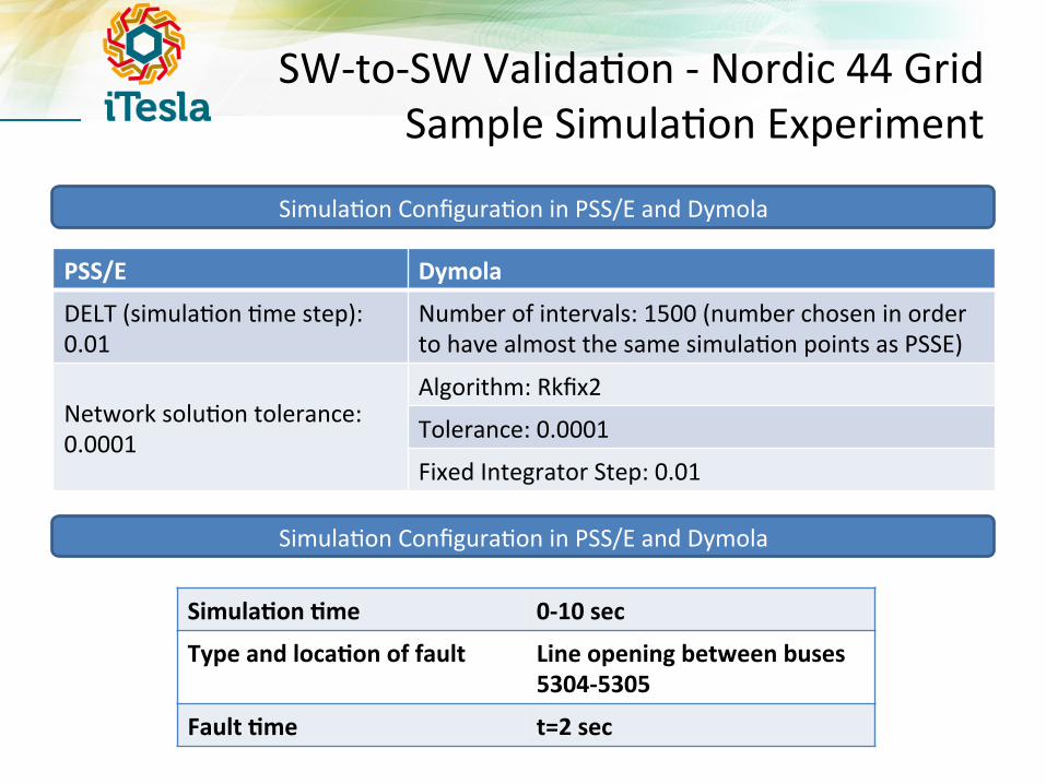
SW-‐to-‐SW Valida5on -‐ Nordic 44 Grid Sample Simula5on Experiment

PSS/E Dymola

DELT (simula5on 5me step): 0.01

Number of intervals: 1500 (number chosen in order to have almost the same simula5on points as PSSE)

Network solu5on tolerance: 0.0001

Algorithm: Rkfix2

Tolerance: 0.0001

Fixed Integrator Step: 0.01

Simula:on :me 0-‐10 sec

Type and loca:on of fault Line opening between buses 5304-‐5305

Fault :me t=2 sec

Simula5on Configura5on in PSS/E and Dymola

Simula5on Configura5on in PSS/E and Dymola

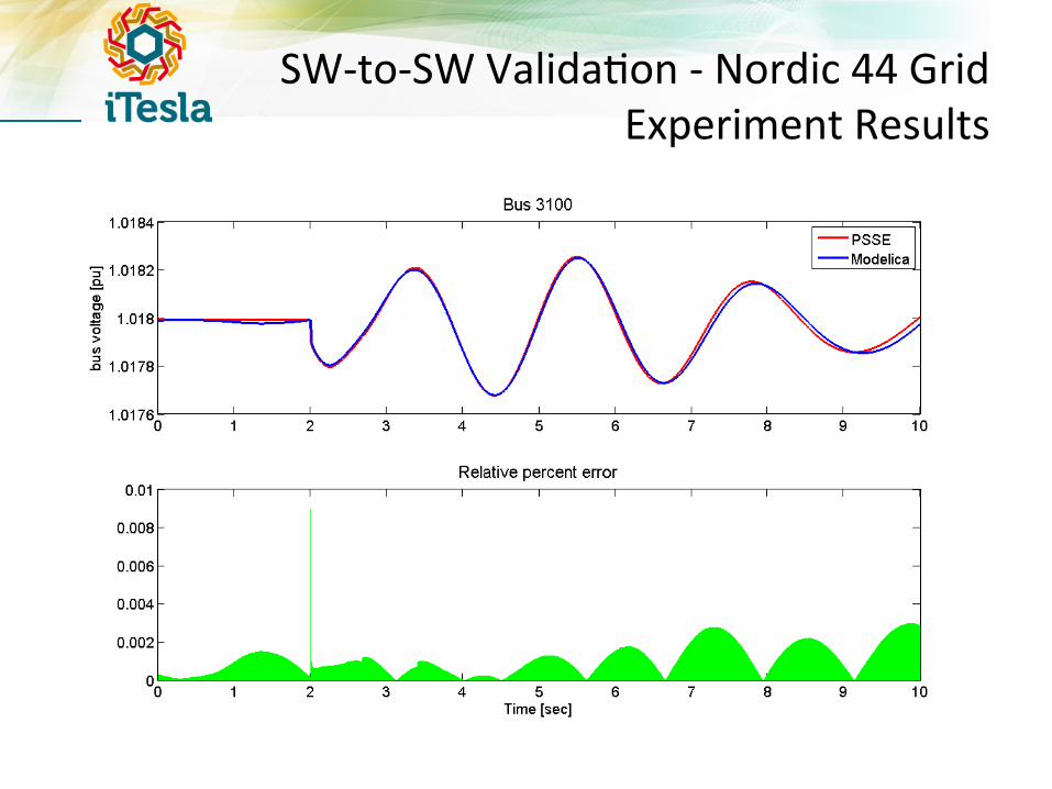
SW-‐to-‐SW Valida5on -‐ Nordic 44 Grid Experiment Results

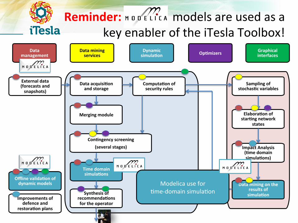
Reminder: models are used as a key enabler of the iTesla Toolbox!

Sampling of stochas:c variables

Elabora:on of star:ng network

states

Impact Analysis (:me domain simula:ons)

Data mining on the results of simula:on


Merging module

Con:ngency screening (several stages)

Time domain simula:ons

Computa:on of security rules



Improvements of defence and

restora:on plans

Offline valida:on of dynamic models

Data management

Data mining services

Dynamic simula:on Op:mizers Graphical

interfaces

Modelica use for 5me-‐domain simula5on

THE RAPID TOOLBOX

Mock-‐Up SoTware Prototype for Component and Aggregate Level Model Valida5on

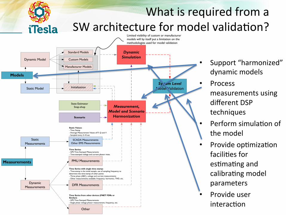
What is required from a SW architecture for model valida5on?

Models

Static Model

Standard Models

Custom Models

Manufacturer Models

System LevelModel Validation

Measurements

Static Measurements

Dynamic Measurements

PMU Measurements

DFR Measurements

Other

Measurement, Model and Scenario

Harmonization

Dynamic Model

SCADA MeasurementsOther EMS Measurements

Static Values:- Time Stamp- Average Measurement Values of P, Q and V- Sampled every 5-10 sec

Time Series:- GPS Time Stamped Measurements- Time-stamped voltage and current phasor meas.

Time Series with single time stamp:- Time-stamp in the initial sample, use of sampling frequency to determine the time-stamp of other points- Three phase (ABC), voltage and current measurements- Other measurements available: frequency, harmonics, THD, etc.

Time Series from other devices (FNET FDRs or Similar):- GPS Time Stamped Measurements- Single phase voltage phasor measurement, frequency, etc.

Scenario

Initialization

State Estimator Snap-shop

DynamicSimulation

Limited visibility of custom or manufacturer models will by itself put a limitation on the methodologies used for model validation

•  Support “harmonized” dynamic models

•  Process measurements using different DSP techniques

•  Perform simula5on of the model

•  Provide op5miza5on facili5es for es5ma5ng and calibra5ng model parameters

•  Provide user interac5on

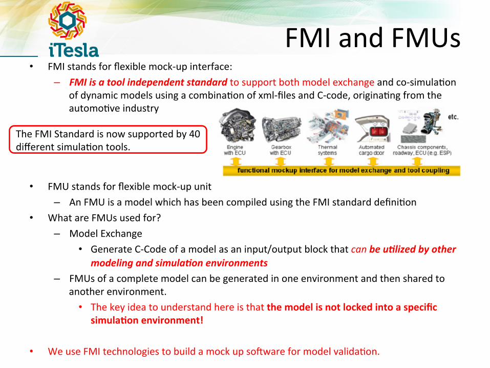
FMI and FMUs •  FMI stands for flexible mock-‐up interface:

–  FMI is a tool independent standard to support both model exchange and co-‐simula5on of dynamic models using a combina5on of xml-‐files and C-‐code, origina5ng from the automo5ve industry

•  FMU stands for flexible mock-‐up unit –  An FMU is a model which has been compiled using the FMI standard defini5on

•  What are FMUs used for? –  Model Exchange

•  Generate C-‐Code of a model as an input/output block that can be u)lized by other modeling and simula)on environments

–  FMUs of a complete model can be generated in one environment and then shared to another environment.

•  The key idea to understand here is that the model is not locked into a specific simula:on environment!

•  We use FMI technologies to build a mock up soTware for model valida5on.

The FMI Standard is now supported by 40 different simula5on tools.

User Target (server/pc)

Model Valida:on Solware

iTesla WP2 Inputs to WP3: Measurements & Models

Mockup SW Architecture Proof of concept of using MATLAB+FMI

EMTP-‐RV and/or other HB model simula:on traces and simula:on configura:on

PMU and other available HB measurements

SCADA/EMS Snapshots + Operator Ac:ons

MAT

LAB

MATLAB/Simulink (used for simula5on of the Modelica Model in FMU format)

FMI Toolbox for MATLAB (with Modelica model)

Model Valida)on Tasks:

Parameter tuning, model op5miza5on, etc.

User Interac5on

.mat and .xml files

HARMONIZED MODELICA MODEL: Modelica Dynamic Model Defini:on for Phasor Time Domain Simula:on

Data Condi5oning

iTesla Data Manager

Internet or LAN .mo files

.mat and .xml files

FMU compiled by another tool

FMU

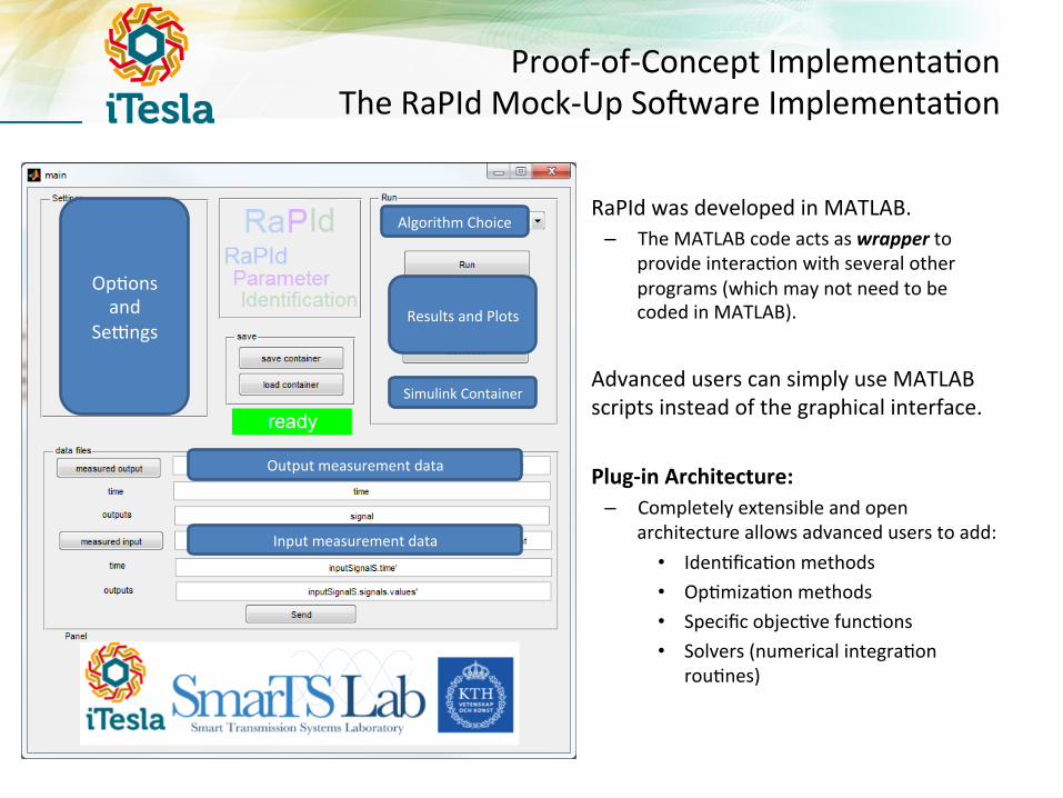
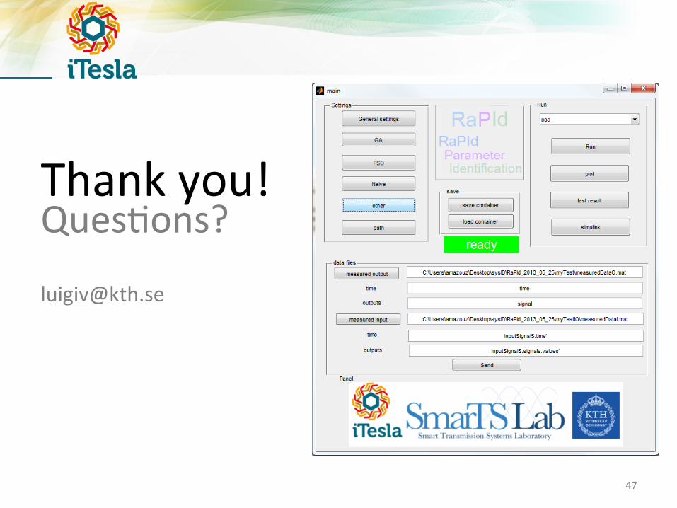
Proof-‐of-‐Concept Implementa5on The RaPId Mock-‐Up SoTware Implementa5on

•  RaP Id i s ou r p roo f o f concep t implementa5on (prototype) of a soTware tool for model es5ma5on and valida5on. The tool provides a framework for model i d en5fi ca5on / v a l i d a5on , ma i n l y parameter iden5fica5on.

•  RaPId is based on Modelica and FMI – applicable to other systems, not only power systems!

•  A Modelica model is fed through an Flexible Mock-‐Unit (i.e. FMU) to Simulink.

•  The model is simulated and its outputs are compared against measurements.

•  RaPId tunes the parameters of the model while minimizing a fitness criterion between the outputs of the simula5on and the experimental measurements of the same outputs provided by the user.

•  RaPId was developed in MATLAB. –  The MATLAB code acts as wrapper to

provide interac5on with several other programs (which may not need to be coded in MATLAB).

•  Advanced users can simply use MATLAB scripts instead of the graphical interface.

•  Plug-‐in Architecture: –  Completely extensible and open

architecture allows advanced users to add: •  Iden5fica5on methods •  Op5miza5on methods •  Specific objec5ve func5ons •  Solvers (numerical integra5on

rou5nes)

Op5ons and

Se2ngs

Algorithm Choice

Results and Plots

Simulink Container

Output measurement data

Input measurement data

What does RaPId do?

Output (and op5onally input) measurements are provided to RaPId by the user.

At ini5aliza5on, a set of parameters is pre-‐configured (or generated randomly by RaPId)

The model is simulated with the parameter values given by RaPId.

The outputs of the model are recorded and compared to the user-‐provided measurements

A fitness func5on is computed to judge how close the measured data and simulated data are to each other

Using results from (5) a new set of parameters is computed by RaPId.

1

2

3

4

5

2’

ymeas

t

ymeas , ysim

tSimulink Container With Modelica FMU Model

Simula:ons con:nue un:l a min. fitness or max no. of itera:ons (simula:on runs) are reached.

1

2

3

4

5

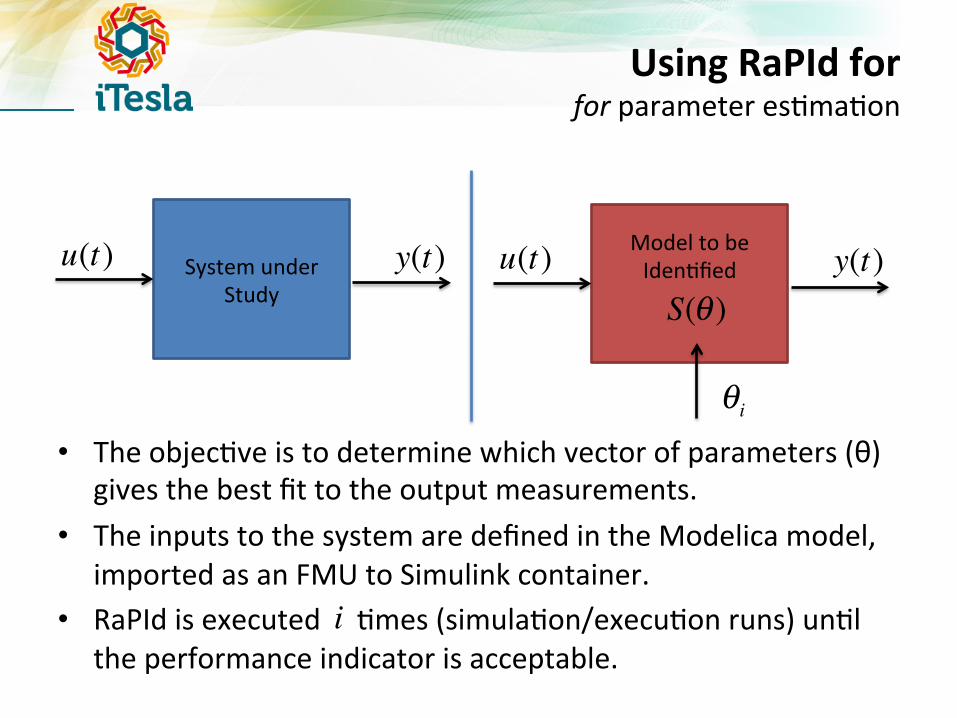
Using RaPId for for parameter es5ma5on

System under Study

Model to be Iden5fied

u(t) y(t) u(t) y(t)

θi

S(θ )

•  The objec5ve is to determine which vector of parameters (θ) gives the best fit to the output measurements.

•  The inputs to the system are defined in the Modelica model, imported as an FMU to Simulink container.

•  RaPId is executed 5mes (simula5on/execu5on runs) un5l the performance indicator is acceptable.

i

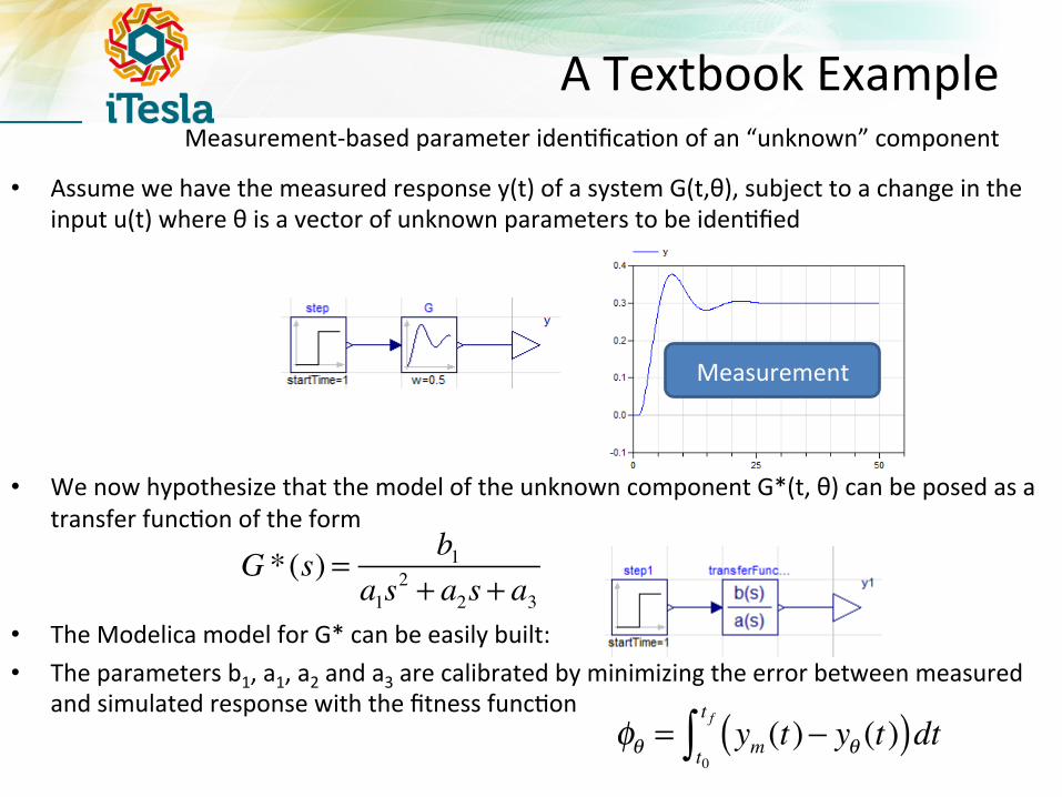
•  Assume we have the measured response y(t) of a system G(t,θ), subject to a change in the input u(t) where θ is a vector of unknown parameters to be iden5fied

•  We now hypothesize that the model of the unknown component G*(t, θ) can be posed as a transfer func5on of the form

•  The Modelica model for G* can be easily built: •  The parameters b1, a1, a2 and a3 are calibrated by minimizing the error between measured

and simulated response with the fitness func5on

A Textbook Example

Measurement-‐based parameter iden5fica5on of an “unknown” component

Measurement

φθ = ym (t)− yθ (t)( )dtt0

t f∫

G *(s) = b1a1s

2 + a2s + a3

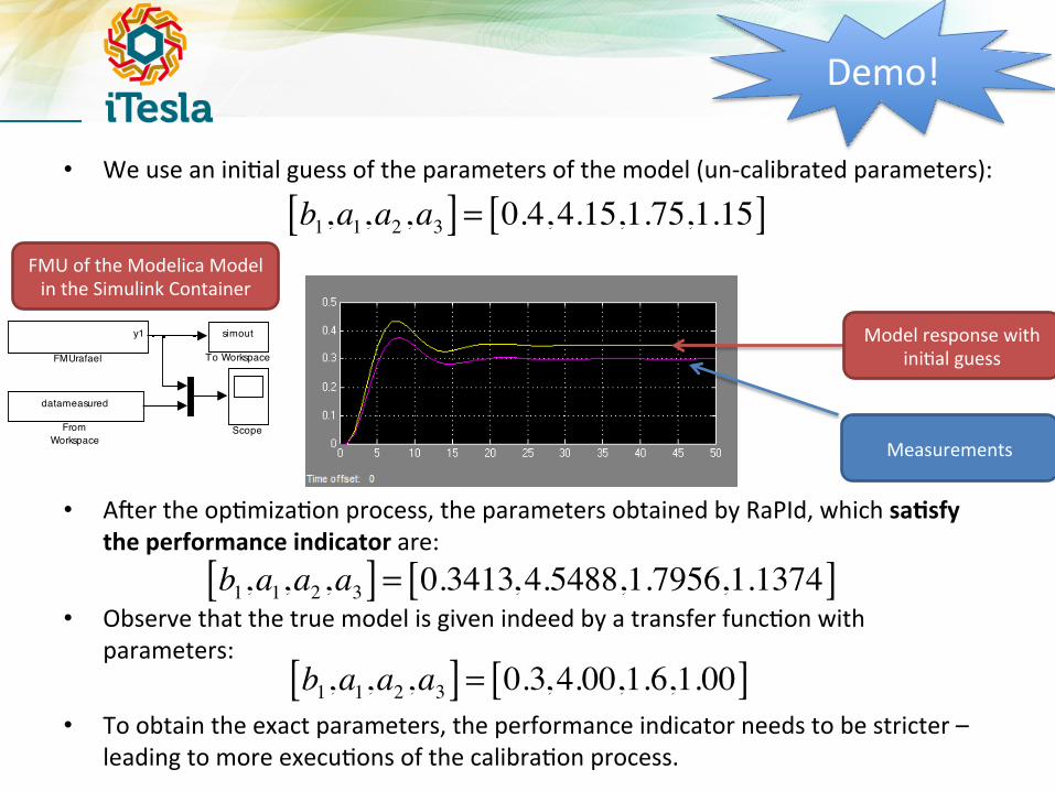
Measurements

Model response with ini5al guess

Demo!

simout

To Workspace

Scope

datameasured

FromWorkspace

y1

FMUrafael

FMU of the Modelica Model in the Simulink Container

•  We use an ini5al guess of the parameters of the model (un-‐calibrated parameters):

•  ATer the op5miza5on process, the parameters obtained by RaPId, which sa:sfy the performance indicator are:

•  Observe that the true model is given indeed by a transfer func5on with parameters:

•  To obtain the exact parameters, the performance indicator needs to be stricter – leading to more execu5ons of the calibra5on process.

b1,a1,a2,a3[ ] = 0.4,4.15,1.75,1.15[ ]

b1,a1,a2,a3[ ] = 0.3413,4.5488,1.7956,1.1374[ ]

b1,a1,a2,a3[ ] = 0.3,4.00,1.6,1.00[ ]

THE RAPID TOOLBOX Applica5on Examples of

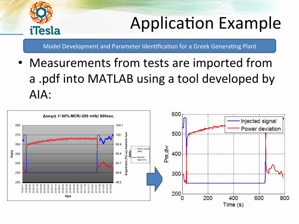
Applica5on Example

•  Measurements from tests are imported from a .pdf into MATLAB using a tool developed by AIA:

Δοκιµή 1/ 60% MCR/-200 mHz/ 900sec.

220

230

240

250

260

270

280

19:5

8:11

19:5

8:58

19:5

9:45

20:0

0:32

20:0

1:19

20:0

2:06

20:0

2:53

20:0

3:40

20:0

4:27

20:0

5:14

20:0

6:01

20:0

6:48

20:0

7:35

20:0

8:22

20:0

9:09

20:0

9:56

20:1

0:43

20:1

1:30

20:1

2:17

20:1

3:04

20:1

3:51

20:1

4:38

20:1

5:25

20:1

6:12

20:1

6:59

Ώρα

Ισχύς

99.5

99.6

99.7

99.8

99.9

100

100.1Συχνότητα

(%) ως ποσοτό των

50H

z

Pow er output(MW)

InjectedSignal (%)

Model Development and Parameter Iden5fica5on for a Greek Genera5ng Plant

Objec5ve: To es5mate p={R, Ts} by minimiza5on of the fitness func5on:

iGrGen Model

where:

FMU in Simulink for RaPId

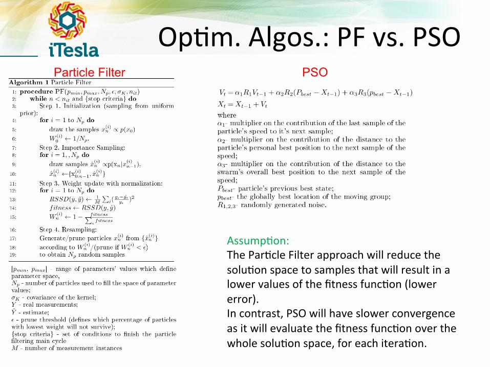
Op5m. Algos.: PF vs. PSO Particle Filter PSO

Assump5on: The Par5cle Filter approach will reduce the solu5on space to samples that will result in a lower values of the fitness func5on (lower error). In contrast, PSO will have slower convergence as it will evaluate the fitness func5on over the whole solu5on space, for each itera5on.

iGrGen Model Iden5fica5on/Valida5on

Video Demo!

Using RaPId’s Command Line and integra5on of a user-‐implemented

op5miza5on method (Par5cle Filtering)

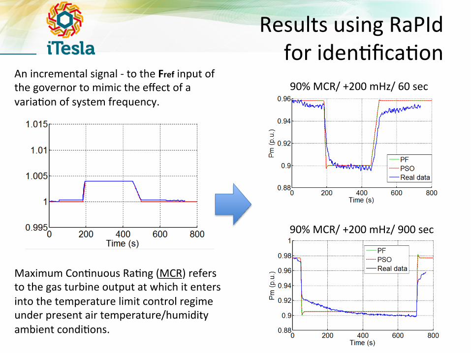
Results using RaPId for iden5fica5on

Maximum Con5nuous Ra5ng (MCR) refers to the gas turbine output at which it enters into the temperature limit control regime under present air temperature/humidity ambient condi5ons.

90% MCR/ +200 mHz/ 60 sec An incremental signal -‐ to the Fref input of the governor to mimic the effect of a varia5on of system frequency.

90% MCR/ +200 mHz/ 900 sec

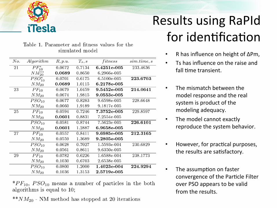
Results using RaPId for iden5fica5on •  R has influence on height of ΔPm, •  Ts has influence on the raise and

fall 5me transient.

•  The mismatch between the model response and the real system is product of the modeling adequacy.

•  The model cannot exactly reproduce the system behavior.

•  However, for prac5cal purposes, the results are sa5sfactory.

•  The assump5on on faster convergence of the Par5cle Filter over PSO appears to be valid from the results.

WP3 IT’S RELEVANCE TO DSA TOOLS OF THE FUTURE

Conclussions

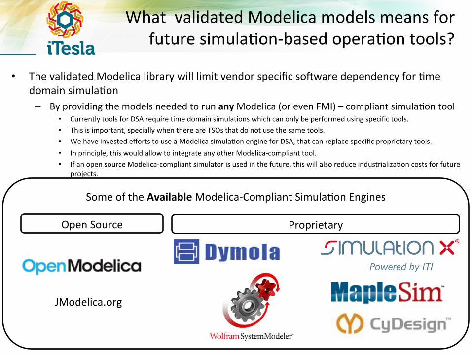
What validated Modelica models means for future simula5on-‐based opera5on tools?

•  The validated Modelica library will limit vendor specific soTware dependency for 5me domain simula5on

–  By providing the models needed to run any Modelica (or even FMI) – compliant simula5on tool •  Currently tools for DSA require 5me domain simula5ons which can only be performed using specific tools. •  This is important, specially when there are TSOs that do not use the same tools. •  We have invested efforts to use a Modelica simula5on engine for DSA, that can replace specific proprietary tools. •  In principle, this would allow to integrate any other Modelica-‐compliant tool. •  If an open source Modelica-‐compliant simulator is used in the future, this will also reduce industrializa5on costs for future

projects.

WP2 -‐ Data Management

On-‐line Workflow

Off-‐line Workflow

WP2 Dynamic Database

Power System Model Defini5on in Modelica

iTesla Modelica Model Library

Model Valida5on Tools

WP3

Model validation results, including validation metrics and parameters are sent back to the dynamic database which

updates these specifications

The Dynamic Database “assigns” classes from

the library

WP4 WP5

Modelica Simula5on Engine

Modelica Simula5on Engine

Some of the Available Modelica-‐Compliant Simula5on Engines

JModelica.org

Open Source Proprietary

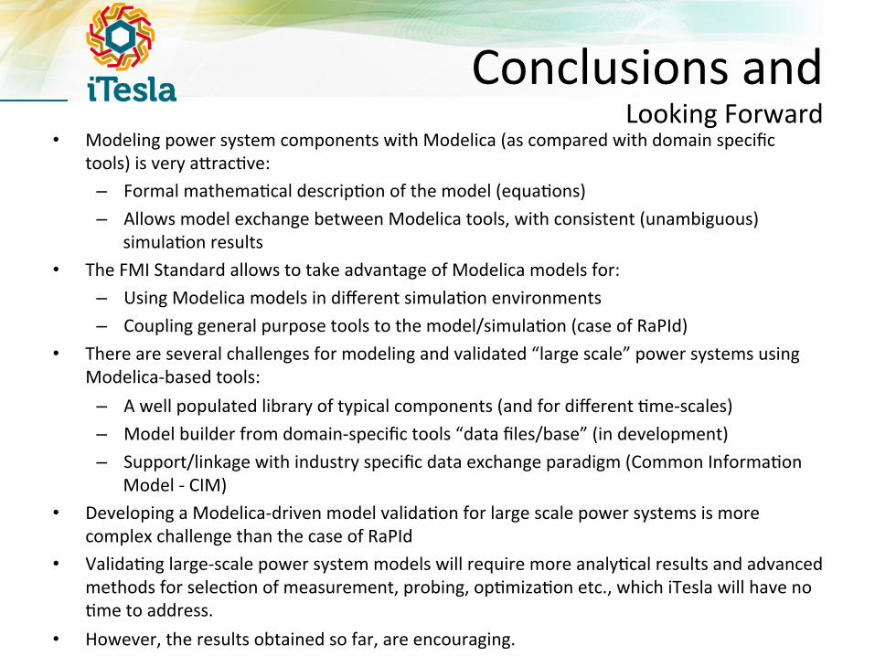
Conclusions and Looking Forward

•  Modeling power system components with Modelica (as compared with domain specific tools) is very aDrac5ve:

–  Formal mathema5cal descrip5on of the model (equa5ons) –  Allows model exchange between Modelica tools, with consistent (unambiguous)

simula5on results •  The FMI Standard allows to take advantage of Modelica models for:

–  Using Modelica models in different simula5on environments –  Coupling general purpose tools to the model/simula5on (case of RaPId)

•  There are several challenges for modeling and validated “large scale” power systems using Modelica-‐based tools:

–  A well populated library of typical components (and for different 5me-‐scales) –  Model builder from domain-‐specific tools “data files/base” (in development) –  Support/linkage with industry specific data exchange paradigm (Common Informa5on

Model -‐ CIM) •  Developing a Modelica-‐driven model valida5on for large scale power systems is more

complex challenge than the case of RaPId •  Valida5ng large-‐scale power system models will require more analy5cal results and advanced

methods for selec5on of measurement, probing, op5miza5on etc., which iTesla will have no 5me to address.

•  However, the results obtained so far, are encouraging.

Ques5ons?

[email protected]

Thank you!

47

iTesla’–Enabling’Resiliency’for’Future’Power’Grids ... ·...

Documents

Transcript of iTesla’–Enabling’Resiliency’for’Future’Power’Grids ... ·...