Iterative Scaling Algorithm for

Channels

Paolo Perrone∗1 and Nihat Ay1,2,3

1Max Planck Institute for Mathematics in the Sciences, Inselstrasse 22, 04103Leipzig, Germany

2Faculty of Mathematics and Computer Science, University of Leipzig, PF 100920,04109 Leipzig, Germany

3Santa Fe Institute, 1399 Hyde Park Road, Santa Fe, NM 87501, USA

Abstract

Here we define a procedure for evaluating KL-projections (I- and rI-projections) of channels. These can be useful in the decomposition ofmutual information between input and outputs, e.g. to quantify synergiesand interactions of different orders, as well as information integration andother related measures of complexity.

The algorithm is a generalization of the standard iterative scaling al-gorithm, which we here extend from probability distributions to channels(also known as transition kernels).

Keywords: Markov Kernels, Hierarchy, I-Projections, Divergences, In-teractions, Iterative Scaling, Information Geometry.

1 Introduction

Here we present an algorithm to compute projections of channels onto exponen-tial families of fixed interactions.

The decomposition is geometrical, and it is based on the idea that, ratherthan joint distributions, the quantities we work with are channels, or condition-als (or Markov kernels, stochastic kernels, transition kernels, stochastic maps).Our algorithm can be considered a channel version of the iterative scaling of(joint) probability distributions, presented in [1].

Exponential and mixture families (of joints and of channels) have a dualityproperty, shown in Section 2. By fixing some marginals, one determines amixture family. By fixing (Boltzmann-type) interactions, one determines anexponential family. These two families intersect in a single point, which means

∗Correspondence: perrone@mis.mpg.de

arX

iv:1

603.

0718

1v1

[cs

.IT

] 2

3 M

ar 2

016

that (Theorem 2) there exists a unique element which has the desired marginalsand the desired interactions.

As a consequence, it translates projections onto exponential families (whichare generally hard to compute) to projections onto fixed-marginals mixture fam-ilies (which can be approximated by an iterative procedure). Section 3 explainshow this is done.

Projections onto exponential families are becoming more and more impor-tant in the definition of measures of statistical interaction, complexity, synergy,and related quantities. In particular, the algorithm can be used to computedecompositions of mutual information, as for example the ones defined in [2]and [3], and it was indeed used to compute all the numerical examples in [3].Another application of the algorithm is explicit computations of complexitymeasure as treated in [4], [5], [6], and [7]. Examples of both applications can befound in Section 4.

For all the technical details about the iterative scaling algorithm, in itstraditional version, we refer the interested reader to [1].

All proofs can be found in the Appendix.

1.1 Technical Definitions

We take the same definitions and notations as in [3], except that we let theoutput be multiple. More precisely, we consider a set of N input nodes V ,taking values in the sets X1, . . . , XN , and a set of M output nodes W , takingvalues in the sets Y1, . . . , YM . We write the input globally as X := X1×· · ·×XN ,and the output globally as Y := Y1 × · · · × YM . We denote by F (Y ) the set ofreal functions on Y , and by P (X) the set of probability measures on X.

Definition 1. Let I ⊆ V and J ⊆ W . We call FIJ the space of functions whoonly depend on XI and YJ :

FIJ :={f ∈ F (X,Y )

∣∣f(xI , xIc , yJ , yJc) = f(xI , x

′Ic , yJ , y

′Jc) ∀xIc , x′Ic , yJc , y′Jc

}. (1)

We can model the channel from X to Y as a Markov kernel k, that assignsto each x ∈ X a probability measure on Y (for a detailed treatment, see [8]).Here we will consider only finite systems, so we can think of a channel simplyas a transition matrix (or stochastic matrix), whose rows sum to one.

k(x; y) ≥ 0 ∀x, y;∑y

k(x; y) = 1 ∀x . (2)

The space of channels from X to Y will be denoted by K(X;Y ). We will denoteby X and Y also the corresponding random variables, whenever this does notlead to confusion.

Conditional probabilities define channels: if p(X,Y ) ∈ P (X,Y ) and themarginal p(X) is strictly positive, then p(Y |X) ∈ K(X;Y ) is a well-defined

channel. Viceversa, if k ∈ K(X;Y ), given p ∈ P (X) we can form a well-definedjoint probability:

pk(x, y) := p(x) k(x; y) ∀x, y . (3)

To extend the notion of divergence from probability distributions to chan-nels, we need an “input distribution”:

Definition 2. Let p ∈ P (X), let k,m ∈ K(X;Y ). Then:

Dp(k||m) :=∑x,y

p(x) k(x; y) logk(x; y)

m(x; y). (4)

Let p, q be joint probability distributions on X × Y , and let D be the KL-divergence. Then:

D(p(X,Y )||q(X,Y )) = D(p(X)||q(X)) +Dp(X)(p(Y |X)||q(Y |X)) . (5)

2 Families of Channels

Suppose we have a family E of channels, and a channel k that may not be in E .Then we can define the “distance” between k and E in terms of Dp.

Definition 3. Let p be an input distribution. The divergence between a channelk and a family of channels E is given by:

Dp(k|| E) := infm∈E

Dp(k||m) . (6)

If the minimum is uniquely realized, we call the channel

πEk := arg minm∈E

Dp(k||m) (7)

the rI-projection of k on E (and simply “an” rI-projection if it is not unique).

The families considered here are of two types, dual to each other: linear andexponential. For both cases, we take the closures, so that the minima definedabove always exist.

Definition 4. A mixture family of K(X;Y ) is a subset of K(X;Y ) definedby an affine equation, i.e., the locus of the k which satisfy a (finite) system ofequations in the form: ∑

x,y

k(x; y)fi(x, y) = ci , (8)

for some functions fi ∈ F (X,Y ), and some constants ci.

Example. Consider a channel m ∈ K(X;Y1, Y2). We can form the marginal:

m(x; y1) :=∑y2

m(x; y1, y2) . (9)

The channels k ∈ K(X;Y1, Y2) such that k(x; y1) = m(x; y1) form a mixturefamily, defined by the system of equations (for all x′ ∈ X, y′1 ∈ Y1):∑

x,y1,y2

k(x; y1, y2) δ(x, x′)δ(y1, y′1) = m(x′; y′1) , (10)

where the function δ(z, z′) is equal to 1 for z = z′, and zero for any other case.More examples of channel marginals will appear in the next section.

Definition 5. A (closed) exponential family of K(X;Y ) is (the closure of) asubset of K(X;Y ) of strictly positive solutions to a log-affine equation, i.e., thelocus of the k which satisfy a (finite) system of equations in the form:∏

x,y

k(x; y)fi(x,y) = ci , (11)

for some functions fi ∈ F (X,Y ), and some constants ci.

This is a multiplicative equivalent of mixture families. For strictly positive k,logarithms are defined, and equation (11) is equivalent to say that log k satisfiesequation (8). However, strictly positive channels do not form a compact space.

Example. Consider the space K(X;Y ). Constant channels (i.e. for which Ydoes not depend on X) form an exponential family, defined by the system ofequations (for all x′ ∈ X, y′ ∈ Y ):∏

x,y

k(x; y)(δ(x,x′)−1)(δ(y,y′)−1) = 1 . (12)

Here is why. The product above is equivalent to write:

k(x; y) k(x′; y) k(x; y′) k(x′; y′) = 1 , (13)

whose strictly positive solutions satisfy:

k(x; y)

k(x; y′)=

k(x′; y)

k(x′; y′), (14)

so that the fraction of elements mapped to y does not depend on x.We now want to show how to construct families which are, in some sense,

dual.

Proposition 1. Let L be a (finite-dimensional) linear subspace of F (X,Y ). Letp ∈ P (X) and k ∈ K(X;Y ). Define:

M(k,L) :=

{m ∈ K(X;Y )

∣∣∣∣∑x,y

m(x; y)l(x, y) =∑x,y

k(x; y)l(x, y) ∀l ∈ L},

(15)and:

E(k,L) :=

{el(x,y)

Z(x)k(x; y)

∣∣∣∣Z(x) =∑y

el(x,y) k(x; y), l ∈ L}. (16)

Then:

1. M(k,L) is a mixture family;

2. E(k,L) is an exponential family.

The duality is expressed by the following result.

Theorem 2. Let L be a subspace of F (X,Y ). Let p ∈ P (X) be strictly positive.Let k0 ∈ K(X;Y ) be a strictly positive “reference” channel. Let E := E(k0,L)and M :=M(k,L). For k′ ∈ K(X;Y ), the following conditions are equivalent:

1. k′ ∈M∩E.

2. k′ ∈ E, and Dp(k||k′) = infm∈E Dp(k||m).

3. k′ ∈M, and Dp(k′||k0) = infm∈MDp(m||k0).

In particular, k′ is unique, and it is exactly πEk.

Geometrically, we are saying that k′ = πEk, the rI-projection of k on E . Wecall the mapping k → k′ the rI-projection operator, and the mapping k0 → k′

the I-projection operator These are the channel equivalent of the I-projectionsintroduced in [9] and generalized in [10]. The result is illustrated in Figure 1.

k

k0k'

Ɛ

M

Figure 1: Illustration of Theorem 2. The point k′ at the intersection minimizeson E the distance from k, and minimizes on M the distance from k0.

I- and rI-projections on exponential families satisfy a Pythagoras-type equal-ity (see Figure 2). For any m ∈ E , with E exponential family:

Dp(k||m) = Dp(k||πEk) +Dp(πEk||m) . (17)

This statement follows directly from the analogous statement for probabilitydistribution found in [11], after applying (5).

k

mπƐ k

Ɛ

Figure 2: Illustration of equation (17).

3 Algorithm

The algorithm can be considered as a channel equivalent of the iterative scalingprocedure (see for example [1]). The computations in the algorithm are iteratedmany times, but as they are mostly array rescalings, they are well-suited forparallelization.

The intuitive idea is the following. Theorem 2 implies that the rI-projectionof k on an exponential family E is the channel minimizing the divergence froma reference channel k0 ∈ E , with constraints on the marginals. We can thenobtain the rI-projection of k with the following trick: rescaling the marginals ofk0, while keeping the divergence as low as possible. Adjusting several marginalsat once is not an easy task, but it can be obtained iteratively.

To apply the theorem, we choose as mixture familyM a family of prescribedmarginals. Marginals of a channel have to be defined, and they depend on theinput distribution.

Definition 6. Let I ⊆ [N ], J ⊆ [M ], J 6= ∅. We define the marginal operatorfor channels as:

k(x; y) 7→ k(xI ; yJ) :=∑

xIc ,yJc

p(xIc |xI) k(xI , xIc ; yJ , yJc) , (18)

for some input probability distribution p. This way, k(XI ;YJ) is exactly theconditional probability for the marginal pk(XI , YJ).

Definition 7. Let I ⊆ [N ], J ⊆ [M ], J 6= ∅. We define the mixture familiesMIJ(k) as:

MIJ(k) :={k(x1...n; y1...m)

∣∣ p(xI) k(xI ; yJ) = p(xI) k(xI ; yJ)}, (19)

where the k(xI ; yJ) are prescribed channel marginals, for a strictly positive inputdistribution p.

Proposition 3. MIJ(k) corresponds exactly to the set M(k,L) defined inProposition 1, where as L we take the space FIJ of functions which only de-pend on the nodes in I, J .

Just as in [1], the I-projections for single marginals can be obtained by‘scaling:

Definition 8. We define the IJ-scaling as the operator σIJ : K(X;Y ) →K(X;Y ), mapping k to:

1

Z(x)k(xI , xIc ; yJ , yJc)

k(xI ; yJ)

k(xI ; yJ), (20)

where:

Z(x) :=∑y′J

k(xI , xIc ; y′J)k(xI ; y

′J)

k(xI ; y′J). (21)

The scaling leaves the input distribution unchanged.

This operation indeed yields an element of the desired family:

Proposition 4. Let k ∈ K(X;Y ). Then σIJk ∈MIJ(k).

The IJ-scaling indeed yields projections, for which a Pythagoras-type rela-tion holds. This means that IJ-scalings are indeed I-projections.

Lemma 5. Let k ∈ K(X;Y ), let m ∈MIJ(k). Let p be a strictly positive inputdistribution. Then:

Dp(m||k) = Dp(m||σIJ k) +Dp(σIJ k||k) . (22)

Corollary 6. σIJ is an I-projection:

Dp(σIJ k||k) = minm∈MIJ (k)

Dp(m||k) . (23)

To prescribe all marginals together, we need to iterate all scalings. Thesequence will then converge to the desired channel.

Definition 9. LetM1, . . . ,Mn be mixture families in K(X;Y ), and denote theI-projection operators as σ1, . . . , σn. Let k0 ∈ K(X;Y ). We call the iterativescaling of k0 the infinite sequence starting at k0, defined inductively by:

ki := σ(imodn) ki−1 . (24)

In our case, we choose the linear families as families of prescribed marginalsfor different subsets of the nodes. That is, Mi =MIiJi(k), with Ii ⊆ [N ] andJi ⊆ [M ], J 6= ∅ for all i.

Theorem 7. If M :=M1 ∩ · · · ∩Mn 6= ∅, and denote by σ the I-projection onM, then:

limi→∞

ki = σ k. (25)

We do not require the projection to be strictly positive.

This result is illustrated in Figure 3.

k0

M1M2

M3

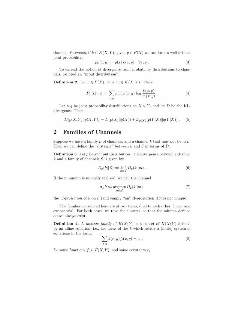
Figure 3: Illustration of the iterative scaling procedure, Theorem 7: subsequentprojections tend to the projection on the intersection of the families.

In our case,, we choose as initial channel k0 exactly the reference channelk0 of Theorem 2. The rI-projection of k on the desired exponential family willbe obtained by the iterative scaling of k0. The limit point will have the sameprescribed marginals as the original kernel k.

4 Applications

4.1 Synergy Measures

The algorithm presented here permits to compute decompositions of mutualinformation between inputs and outputs in [2] and [3]. We give here examples ofcomputations of pairwise synergy as an rI-projection for channels, as describedin [3]. It is not within the scope of this article to motivate this measure, werather want to show how it can be computed.

Let k be a channel from X = (X1, X2) to Y . Let p ∈ P (X) be a strictlypositive input distribution. We define in [3] the synergy of k as:

d2(k) := Dp(k|| E1) , (26)

where E1 is the (closure of the) family of channels in the form:

m(x1, x2; y) =1

Z(X)exp

(φ0(x1, x2) + φ1(x1, y) + φ2(x2, y)

), (27)

where:Z(x) :=

∑y

exp(φ0(x1, x2) + φ1(x1, y) + φ2(x2, y)

), (28)

and:φ0 ∈ F{1,2}∅ , φ1 ∈ F{1}{1} , φ2 ∈ F{2}{1} . (29)

According to Theorem 2, the rI-projection of k on E1 is the unique point k′ ofE1 which has all the prescribed marginals:

k′(x1; y) = k(x1; y) , k′(x2; y) = k(x2; y) , (30)

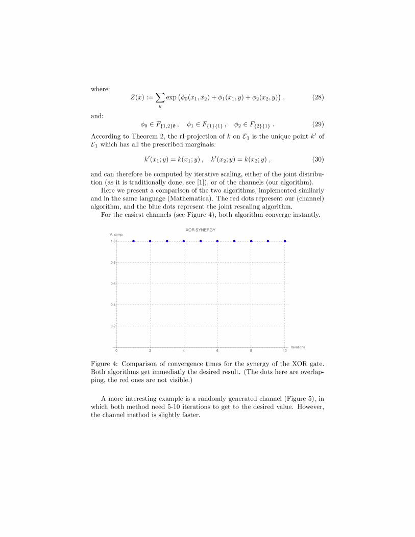
and can therefore be computed by iterative scaling, either of the joint distribu-tion (as it is traditionally done, see [1]), or of the channels (our algorithm).

Here we present a comparison of the two algorithms, implemented similarlyand in the same language (Mathematica). The red dots represent our (channel)algorithm, and the blue dots represent the joint rescaling algorithm.

For the easiest channels (see Figure 4), both algorithm converge instantly.

0 2 4 6 8 10Iterations

0.2

0.4

0.6

0.8

1.0

V. comp.

XOR SYNERGY

Figure 4: Comparison of convergence times for the synergy of the XOR gate.Both algorithms get immediatly the desired result. (The dots here are overlap-ping, the red ones are not visible.)

A more interesting example is a randomly generated channel (Figure 5), inwhich both method need 5-10 iterations to get to the desired value. However,the channel method is slightly faster.

0 2 4 6 8 10Iterations

0.001

0.002

0.003

0.004

0.005

0.006

0.007

V. comp.

RANDOM KERNEL SYNERGY

Figure 5: Comparison of convergence times for the synergy of a randomly gen-erated channel. The channel method (red) is slightly faster.

The most interesting example is the synergy of the AND gate, which shouldbe zero according to the procedure [3]. In that article, we mistakenly wrote adifferent value, that here we would like to correct (it is zero). The convergenceto zero is very slow, of the order of 1/n (Figure 6). It is clearly again slightlyfaster for the channel method in terms of iterations.

0 200 400 600 800 1000Iterations

0.0002

0.0004

0.0006

0.0008

0.0010

0.0012

0.0014

V. comp.

AND SYNERGY

Figure 6: Comparison of convergence times for the synergy of the AND gate.The channel method (red) tends to zero proportionally to n−1.05, the jointmethod (blue) proportionally to n−0.95.

It has to be noted, however, that rescaling a channel requires more elemen-

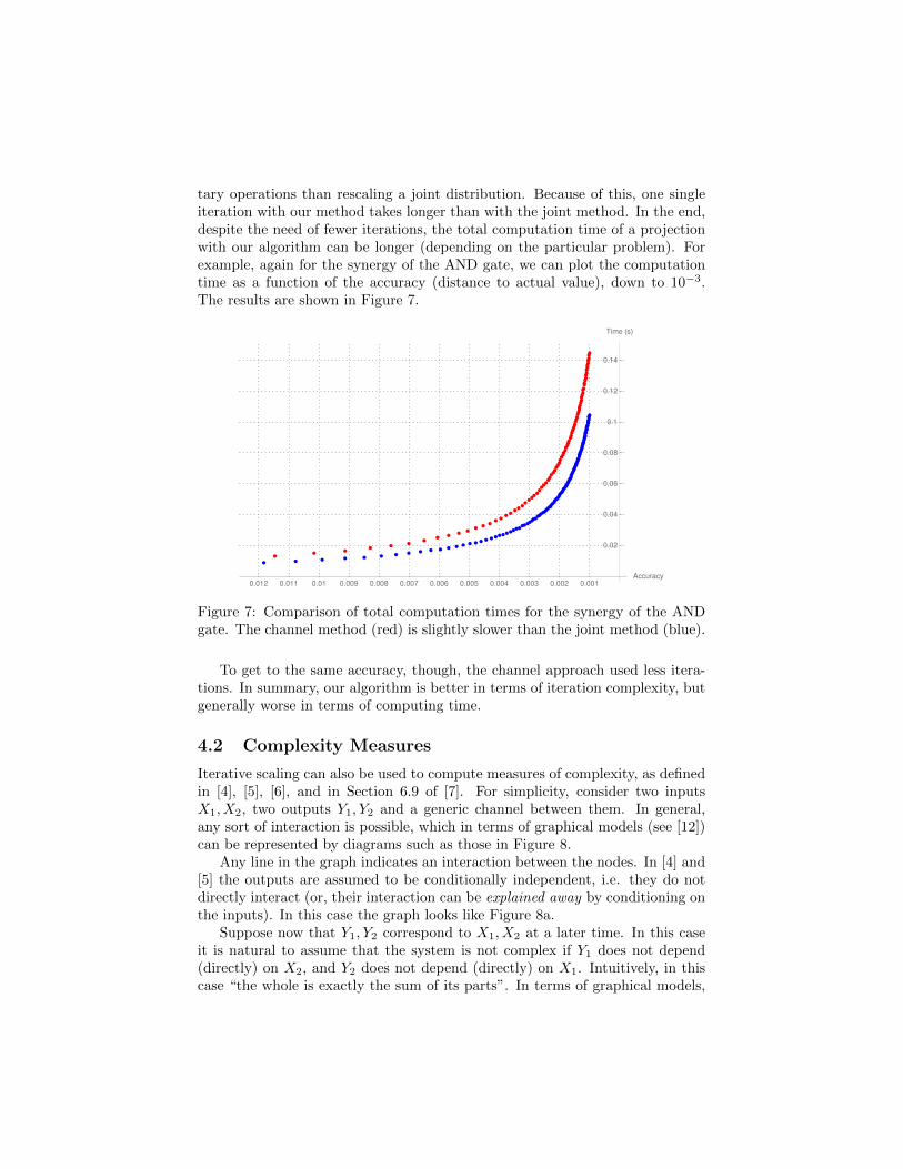
tary operations than rescaling a joint distribution. Because of this, one singleiteration with our method takes longer than with the joint method. In the end,despite the need of fewer iterations, the total computation time of a projectionwith our algorithm can be longer (depending on the particular problem). Forexample, again for the synergy of the AND gate, we can plot the computationtime as a function of the accuracy (distance to actual value), down to 10−3.The results are shown in Figure 7.

0.0010.0020.0030.0040.0050.0060.0070.0080.0090.010.0110.012Accuracy

0.02

0.04

0.06

0.08

0.1

0.12

0.14

Time (s)

Figure 7: Comparison of total computation times for the synergy of the ANDgate. The channel method (red) is slightly slower than the joint method (blue).

To get to the same accuracy, though, the channel approach used less itera-tions. In summary, our algorithm is better in terms of iteration complexity, butgenerally worse in terms of computing time.

4.2 Complexity Measures

Iterative scaling can also be used to compute measures of complexity, as definedin [4], [5], [6], and in Section 6.9 of [7]. For simplicity, consider two inputsX1, X2, two outputs Y1, Y2 and a generic channel between them. In general,any sort of interaction is possible, which in terms of graphical models (see [12])can be represented by diagrams such as those in Figure 8.

Any line in the graph indicates an interaction between the nodes. In [4] and[5] the outputs are assumed to be conditionally independent, i.e. they do notdirectly interact (or, their interaction can be explained away by conditioning onthe inputs). In this case the graph looks like Figure 8a.

Suppose now that Y1, Y2 correspond to X1, X2 at a later time. In this caseit is natural to assume that the system is not complex if Y1 does not depend(directly) on X2, and Y2 does not depend (directly) on X1. Intuitively, in thiscase “the whole is exactly the sum of its parts”. In terms of graphical models,

X1 Y1

X2 Y2

(a)

X1 Y1

X2 Y2

(b)

Figure 8: a) The graphical model corresponding to conditionally independentoutputs Y1 and Y2 are indeed correlated, but only indirectly, via the inputs. b)The graphical model corresponding to a non-complex system.

this means that our system is represented by Figure 8b. These channels (orjoints) form an exponential family (see [4] and [5]) which we call F1.

Suppose now, though, that the outputs are indeed conditionally independent,but that they also depend on additional inputs, which we call X3, that we cannotobserve, and which we can consider as “noise”. The graph would then be thatof Figure 9a. If such a system is not complex (but the noise persists), we thenhave a graphical model as in Figure 9b.

Since we cannot observe the noise alone, we have to integrate (or sum, ormarginalize) over the node X3. This way a “noisy” correlation between theoutput nodes appears (see Figure 10). In particular, since X3 is now “hidden”,the outputs are not conditionally independent anymore. In particular, a non-complex but “noisy” system would be represented by Figure 10b. Such channels(or joints) form again an exponential family, which we call F2.

We would like now to have a measure of complexity for a channel (or joint).In [4] and [5], the measure of complexity is defined as the divergence from thefamily F1 represented in Figure 8b. We will call such a measure c1. In case ofnoise, however, it is argued in [6] and [7] that the divergence should be computedfrom the family F2 represented in 10b, because of the marginalization over thenoise (and, as written in the cited papers, because such a complexity measureshould be required to be upper bounded by the mutual information between Xand Y ). We will call such a measure c2.

Both divergences can be computed with our algorithm. As an example, wehave considered the following channel:

k(x1, x2, x3; y1, y2) =1

Z(x)exp

((αx1 x2 + βx3

)(y1 − y2)

), (31)

X1 Y1

X2 Y2

X3

(a)

X1 Y1

X2 Y2

X3

(b)

Figure 9: a) The model of Figure 8a, with and additional “noise” input term X3.b) The graphical model corresponding to a non-complex system, with possiblenoise.

X1 Y1

X2 Y2

(a)

X1 Y1

X2 Y2

(b)

Figure 10: a) The graphical model of Figure 9a, after marginalizing over thenoise. b) The non-complex model of Figure 9b, after marginalizing over thenoise.

with:

Z(x) =∑y′1,y

′2

exp

((αx1 x2 + βx3

)(y′1 − y′2)

). (32)

We have chosen α = 1 and β = 2, and a uniform input probability p. Aftermarginalizing over X3, we can compute the two divergences:

• c1(k) = Dp(k|| F1) = 0.519.

• c2(k) = Dp(k|| F2) = 0.110.

This indicates that c1 is incorporating the correlation of the output nodes dueto the “noise”, and therefore probably overestimating the complexity, at leastin this case.

One could nevertheless argue that c2 can underestimate complexity, as wecan see in the following “control” example. Consider the channel:

h(x1, x2, x3; y1, y2) =1

Z(x)exp

((αx1 x2

)(y1 − y2)

), (33)

with:

Z(x) =∑y′1,y

′2

exp

((αx1 x2

)(y′1 − y′2)

), (34)

which is represented by the graph in Figure 8a. If the difference between c1 andc2 were just due to the noise, then for our new channel c1(h) and c2(h) shouldbe equal. This is not the case:

• c1(h) = Dp(h|| F1) = 0.946.

• c1(h) = Dp(h|| F2) = 0.687.

The divergences are still different. This means that there is an element h2 inF2, which does not lie in F1, for which:

Dp(h||h2) < Dp(h||h1) ∀h1 ∈ f1 . (35)

The difference is this time smaller, which could mean that noise still doesplay a role, but in rigor it is hard to say, since none of these quantities is linear,and divergences do not satisfy a triangular inequality.

We do not want to argue here in favor or against any of these measures. Wewould rather like to point out that such considerations can be done mostly afterexplicit computations, which can be done with iterative scaling.

References

[1] Csiszar, I. and Shields, P. C. Information Theory and Statistics: A Tuto-rial. Foundations and Trends in Communications and Information Theory,1(4):417–528, 2004

[2] Olbrich, E., Bertschinger, N., and Rauh, J. Information decomposition andsynergy. Entropy, 17(5):3501–3517, 2015

[3] Perrone, P. and Ay, N. Hierarchical quantification of synergy in channels.Frontiers in Robotics and AI, 35(2), 2016.

[4] Ay, N. Information Geometry on Complexity and Stochas-tic Interaction. MPI MiS Preprint, 95/2001. Available online:http://www.mis.mpg.de/publications/preprints/2001/prepr2001-95.html

[5] Ay, N. Information Geometry on Complexity and Stochastic Interaction.Entropy, 17, 2432–2458, 2015.

[6] Oizumi, M., Tsuchiya, N., and Amari, S. A unified framework for infor-mation integration based on information geometry Preprint available onarXiv:1510.04455, 2015.

[7] Amari, S. Information Geometry and Its Applications Springer, 2016.

[8] Kakihara, Y. Abstract Methods in Information Theory. World Scientific,1999.

[9] Csiszar, I. I-divergence geometry of probability distributions and minimiza-tion problems. Annals of Probability, 3:146–158, 1975.

[10] Csiszar, I. and Matus, F. Information projections revisited. IEEE Trans-actions on Information Theory, 49:1474–1490, 2003.

[11] Amari, S. Information geometry on a hierarchy of probability distributions.IEEE Transactions on Information Theory, 47(5):1701–1709, 2001.

[12] Lauritzen, S. L. Graphical Models. Oxford, 1996.

[13] Williams, P. L. and Beer, R. D. Nonnegative decomposition of multivariateinformation. Submitted. Preprint available on arXiv:1004.2151, 2010.

[14] Amari, S. and Nagaoka, H. Differential geometry of smooth families ofprobability distributions. Technical Report METR 82-7, Univ. of Tokyo,1982.

[15] Amari, S. and Nagaoka, H. Methods of Information Geometry. Oxford,1993.

A Proofs

Proof of Proposition 1. Let {fi} be a basis of L, orthonormal in L2 (w.r.t. thecounting measure). Then:

1. The condition in (15) is equivalent to:∑x,y

m(x; y)fi(x, y) =∑x,y

k(x; y)fi(x, y) = ci , (36)

for every i, and for some constants ci, and this is in the form of (8).

2. The elements of E(k,L) are in the form, for some θi:

h(x; y) =k(x; y)

Z(x)exp

(∑i

θifi(x, y)

). (37)

We have, for the exponential term:

∏x,y

exp

(∑i

θifi(x, y)

)fj(x,y)

= exp

(∑i

θi∑x,y

fi(x, y)fj(x, y)

), (38)

which because of orthonormality is equal to:

exp

(∑i

θiδij

)= eθj . (39)

Therefore:

∏x,y

h(x; y)fi(x,y) = eθi

∏x′,y′

k(x′; y′)

Z(x′)

= ci (40)

for some constants ci, which is exactly in the form of (11).

Proof of Theorem 2. 1 ⇔ 2: Choose a basis f0 = 1, f1, . . . , fd of L. Define themap θ 7→ kθ, with:

kθ(x; y) = k(θ1, . . . , θd)(x; y) :=1

Zθ(x)k0(x; y) exp

d∑j=1

θjfj(x, y)

, (41)

and:

Zθ(x) :=∑y

k0(x; y) exp

(d∑i=1

θifi(x, y)

). (42)

Then:

Dp(k||kθ) = Dp(k||k0)−d∑j=1

θj Epk[fj ] + Ep[logZθ] . (43)

Deriving (where ∂j is w.r.t. θj):

∂j Dp(k||kθ) = −Epk[fj ] + Ep[∂j ZθZθ

]. (44)

The term in the last brackets is equal to:

∂j ZθZθ

=1

Zθ

∑y

k0(x; y) exp

(d∑i=1

θifi(x, y)

)fj(x, y) (45)

=∑y

kθ(x; y)fj(x, y) , (46)

so that (44) now reads:

∂j Dp(k||kθ) = −Epk[fj ] + Epkθ [fj ] . (47)

This quantity is equal to zero for every j if and only if kθ ∈ M. Now if kθ isa minimizer, it satisfies (47), and so kθ ∈ M. Viceversa, suppose kθ ∈ M, sothat it satisfies (47) for every j. To prove that it is a global minimizer, we lookat the Hessian:

∂i ∂j Dp(k||kθ) = ∂i ∂j D(pk||pkθ) . (48)

This is precisely the covariance matrix of the joint probability measure pkθ,which is positive definite.

1⇔ 3: For every m ∈M, we have:

Dp(m||k0) =∑x,y

p(x)m(x; y) logm(x; y)

k0(x; y)= Epm

[log

m

k0

]. (49)

If k′ ∈ E , then:

Dp(m||k0) = Epm[log

m

k′+ log

k′

k0

]= Dp(m||k′) + Epm

[log

k′

k0

]. (50)

By definition of E , the logarithm in the last brackets belongs to L, and sincem ∈M:

Epm[log

k′

k0

]= Epk

[log

k′

k0

]= Epk′

[log

k′

k0

]. (51)

Inserting in (50):

Dp(m||k0) = Dp(m||k′) + Epk′[log

k′

k0

]= Dp(m||k′) +Dp(k

′||k0) . (52)

Since Dp(m||k′) ≥ 0, (52) shows that k′ is a minimizer. Since Dp(m||k0) =D(pm||pk0) is strictly convex in the first argument, its minimizer is unique.

Proof of Proposition 3. For f in FIJ :

Epk[f ] =∑x,y

p(x) k(x; y) f(x, y) =∑xI ,yJ

p(xI) k(xI ; yJ) f(xI ; yJ) , (53)

and just as well:

Epk[f ] =∑x,y

p(x) k(x; y) f(x, y) =∑xI ,yJ

p(xI) k(xI ; yJ) f(xI ; yJ) . (54)

The definition in Proposition 1 (with strict positivity of p) requires exactly that:

Epk[f ] = Epk[f ] (55)

for every f ∈ FIJ . Using (53) and (54), the equality becomes:∑xI ,yJ

p(xI) k(xI ; yJ) f(xI ; yJ) =∑xI ,yJ

p(xI) k(xI ; yJ) f(xI ; yJ) (56)

for every f in FIJ , which means that k(xI ; yJ) = k(xI ; yJ).

Proof of Proposition 4. Let p(X) be a strictly positive input distribution. Ap-plying (18) to (20):

(σIJ k)(xI ; yJ) =∑xIc

p(xIc |xI)Z(xI , xIc)

k(xI , xIc ; yJ)k(xI ; yJ)

k(xI ; yJ)

= k(xI ; yJ)∑xIc

p(xIc |xI)Z(xI , xIc)

k(xI , xIc ; yJ)

k(xI ; yJ)

= k(xI ; yJ)∑xIc

1

Z(xI , xIc)

pk(xI , xIc , yJ)

pk(xI , yJ)

= k(xI ; yJ)∑xIc

pk(xIc |xI , yJ)∑y′J

pk(xIc |xI , y′J)

p(x)pk(xI , y′J)

= k(xI ; yJ)∑xIc

pk(xIc |xI , yJ) p(x)∑y′Jpk(xIc |xI , y′J) pk(xI , y′J)

= k(xI ; yJ)∑xIc

pk(xIc |xI , yJ) p(x)

p(x),

as the input probability is the same. We are left with:

(σIJ k)(xI ; yJ) = k(xI ; yJ)∑xIc

pk(xIc |xI , yJ) = k(xI ; yJ) , (57)

which is exactly the constraint of MIJ .

Proof of Lemma 5. Expanding the r.h.s. of (22) with (4), and inserting (20):

Dp(m||σIJ k) +Dp(σIJ k||k)

=∑x,y

p(x)

(m(x; y) log

m(x; y)

σIJ k(x; y)+ σIJ k(x; y) log

σIJ k(x; y)

k(x; y)

)

=∑x,y

p(x)

(m(x; y) log

m(x; y)

k(x; y)

Z(x) k(xI ; yJ)

k(xI ; yJ)+ σIJ k(x; y) log

k(xI ; yJ)

Z(x) k(xI ; yJ)

)=∑x,y

p(x)

(m(x; y) log

m(x; y)

k(x; y)+ log

Z(x) k(xI ; yJ)

k(xI ; yJ)

(m(x; y)− σIJ k(x; y)

))= Dp(m||k) +

∑xI ,yJ

logZ(x) k(xI ; yJ)

k(xI ; yJ)

∑xIc ,yJc

(p(x)m(x; y)− p(x) σIJ k(x; y)

)= Dp(m||k) +

∑xI ,yJ

logZ(x) k(xI ; yJ)

k(xI ; yJ)

(p(xI)m(xI ; yJ)− p(xI) σIJ k(xI ; yJ)

)= Dp(m||k) +

∑xI ,yJ

logZ(x) k(xI ; yJ)

k(xI ; yJ)p(xI)

(k(xI ; yJ)− k(xI ; yJ)

)= Dp(m||k) + 0 ,

as both m and σIJ k belong toMIJ(k) (the latter using Proposition 4), and sothey have the prescribed marginals.

Proof of Theorem (7). The proof is adapted from the analogous statement forprobability distributions found in [1]. Equation (22) implies that for every i, fork ∈M:

Dp(k||ki−1) = Dp(k||ki) +Dp(ki||ki−1) . (58)

Summing these equations for i = 1, . . . , N we get:

Dp(k||k0) = Dp(k||kN ) +

N∑i=1

Dp(ki||ki−1) . (59)

Since the polytope of channels is compact, there exists at least an accumulationpoint k′ and a subsequence kNj → k′. This means:

Dp(k||k0) = Dp(k||k′) +

∞∑i=1

Dp(ki||ki−1) , (60)

so that the series on the right must be convergent, and its terms must tend tozero. This in turn implies, using Pinsker’s inequality:∑

x,y

|kNj (x; y)− kNj−1(x; y)| → 0 , (61)

which means that also the subsequence kNj−1 → k′. So does kNj−2, andso on until kNj−n. Among the terms kNj−1, . . . , kNj−n there is one in each

M1, . . . ,Mn, and since they all tend to the same accumulation point k′, k′

must lie in the intersection M. Therefore (60) holds for k′ as well:

Dp(k′||k0) = 0 +

∞∑i=1

Dp(ki||ki−1) , (62)

which substituted again gives, for any k ∈M:

Dp(k||k0) = Dp(k||k′) +Dp(k′||k0) , (63)

i.e. k′ = σ k0, which is unique for strictly positive p. Since the choice ofsubsequence was arbitrary, σ k0 is the only accumulation point, so the sequenceconverges.