Iteration of holomorphic functions in the complex...
58
Final research project GRAU DE MATEM ` ATIQUES Facultat de Matem` atiques Universitat de Barcelona Iteration of holomorphic functions in the complex plane Author: Albert Millan Carrasco Supervisor: Dra. N´ uria Fagella Rabionet Made at: Departament de Matem` atica Aplicada i An` alisi Barcelona, June 27, 2016
Transcript of Iteration of holomorphic functions in the complex...
Final research project
GRAU DE MATEMATIQUES
Facultat de MatematiquesUniversitat de Barcelona
Iteration of holomorphic functions in
the complex plane
Author: Albert Millan Carrasco
Supervisor: Dra. Nuria Fagella Rabionet
Made at: Departament de
Matematica Aplicada i Analisi
Barcelona, June 27, 2016

Abstract
When a holomorphic function is iterated, it generates a dynamic system on the complex
plane. In this project, we describe both the local and global behavior of the different orbits
of a rational map on the complex plane (or the Riemann sphere). We mainly concentrate
in the study of the dynamical plane (where initial conditions and orbits live) although we
briefly discuss one parameter families of polynomials and their bifurcation loci, like the well
known Mandelbrot set. Towards the end, we experiment with a singular perturbation of a
family of cubic polynomials and explore the drastic changes that occur in the topology of
their Julia sets.
i
Preface
The main motivation for doing this project is my interest in dynamical systems and fractal-
like structures, aside from the fact that the courses I enjoyed the most studying are ”Complex
analysis” and ”Mathematical models and dynamic systems”. It has evolved a lot from the
initial idea to what it has been in the end, as new subjects of interest kept appearing while
studying the originally planed topics.
ii

CONTENTS
Contents
1 INTRODUCTION 1
2 PRELIMINARIES AND TOOLS 6
3 INTRODUCTION AND LOCAL THEORY 11
3.1 INTRODUCTORY RESULTS . . . . . . . . . . . . . . . . . . . . . . . . . . 11
3.2 LOCAL THEORY . . . . . . . . . . . . . . . . . . . . . . . . . . . . . . . . 12
4 GLOBAL THEORY 21
4.1 GENERAL RESULTS . . . . . . . . . . . . . . . . . . . . . . . . . . . . . . 21
4.2 RATIONAL FUNCTIONS . . . . . . . . . . . . . . . . . . . . . . . . . . . . 24
4.2.1 FATOU COMPONENTS, NON-REPELLING CYCLES AND CRIT-
ICAL POINTS . . . . . . . . . . . . . . . . . . . . . . . . . . . . . . 26
4.3 POLYNOMIALS . . . . . . . . . . . . . . . . . . . . . . . . . . . . . . . . . 33
5 QUADRATIC POLYNOMIALS AND THE MANDELBROT SET 37
6 SINGULAR PERTURBATIONS OF CUBIC MILNOR POLYNOMIALS 43
6.1 SINGULAR PERTURBATIONS . . . . . . . . . . . . . . . . . . . . . . . . 43
6.2 MILNOR POLYNOMIALS . . . . . . . . . . . . . . . . . . . . . . . . . . . 44
6.3 SINGULAR PERTURBATIONS OF MILNOR CUBIC POLYNOMIALS . . 47
7 GLOSSARY 51
References 54
iii

1 INTRODUCTION
1 INTRODUCTION
All throughout the history of mankind, both the admiration and interrogation about natural
phenomena and the structure of natural objects have been a common trait. Most of the
ancient civilizations were already fascinated by classical geometrical forms, such as circles
and triangles, and tried to give a rational and reasoned description of natural objects taking
as a starting point these classical forms. Two of the most renowned examples of their
interest and knowledge in classical geometry are the The Elements, a geometry treaty written
by Euclid in the IV century b.C, or the famous welcoming sentence written in Plato 's
academy : ”Let no one ignorant of geometry enter”. However, nature often lacked the most
estimated properties of classical geometry like symmetry, proportion and harmony, making
it impossible to describe the world around us by the only use of classical figures, provided
not extreme simplifications were made, and also leading to errors, such as the assumption
that celestial orbits were perfectly circular. Although it it is true that in the following
centuries some of these errors were corrected, only classical geometry forms were considered
when addressing these problems. It was not until the XIX century, when mathematicians
like Weierstrass1, Koch2 or Cantor3 explored objects whose properties were not explained
by traditional geometry; these objects are known nowadays as fractals. Their studies, due
to the lack of technological means of visualization, and the lack of mathematical knowledge
and background in this area, made their works very abstract.
In the XX century, Poincare4, Schroder5, Fatou or Julia did the first incursions in the world
of iteration in both the euclidean and the complex plane, discovering what we call dynamical
systems, some of which behaved in a chaotic way, that is, similar initial conditions gave place
to very different outcomes when iterated. These dynamical systems, sometimes generated
geometrical objects with properties similar to the fractals studied by Cantor or Koch. How-
ever, the lack of technology, specially computers, proved a liability, as they were not able
1Karl Weierstrass (1815 - 1897) was a German mathematician, who made very important contributions
to the field of analysis, like the definitions of continuity and limit of a function or the proof of the mean
value theorem.2Niels Helge von Koch (1870 - 1924) was a Swedish mathematician, and although he made contributions
to number theory, his most known result is the description of the fractal known as Koch snowflake.3Georg Cantor (1845 - 1918) was a German mathematician. He invented set theory, and among other
results, he announced the theory of transfinite number, which was widely criticized at the time.4Henri Poincare (1854 - 1912) was a French mathematician and theoretical physicist. He is considered by
many ”The Last Universalist”, since he made important contributions to all fields of mathematics. Among his
many results are the Poincare Conjecture, which remained unproven until 2002, and laying the foundations
of chaos theory.5Ernst Schroder (1841 - 1902) was a German mathematician, mostly known by his works in algebraic
logic.
1
1 INTRODUCTION
to see the objects they were facing. The appearance of computers, halfway into the XX
century, and with them the capacity of doing millions of numerical operations by second and
to visualize some of the obtained results, was the top expression of the technological revo-
lution which had started a century earlier with the industrial revolution. These objects, far
from being only an academical curiosity, kept appearing when studying natural phenomena
and the universe that surrounds us, such as snow flakes, thunderbolts or drought-produced
cracks, substituting the interest for classical geometrical objects, and opening a new world of
possibilities. However, the balance was lost again, and many researchers classified as fractals
a lot of objects which, although they presented one of the main properties of a fractal object,
self-similarity, were not fractals.
When referring to iterative methods, Newton’s method is probably the best known of them,
and it is used to compute approximate solutions, either real or complex, of an equation
f(z) = 0
provided f is differentiable. It was described by Isaac Newton in his 1669 book ” De analysi
per aequationes numero terminorum infinitas”. Although Newton’s method and other itera-
tive procedures (some of which were variations of Newton’s method) had been already used
earlier, the first mention of iteration of holomorphic functions is found in a study made by
Schroder about Newton’s method. The greatest difference between his work and the previous
ones is the consideration of the method as the iteration of the map
N(z) = z − f(z)f ′(z)
in the complex plane. In doing so, he observed that the iterating holomorphic functions could
be very useful towards the objective of finding better root-finding methods; in fact, Schroder
proved the result known as Fixed Point Theorem, which explained why Newton’s method
worked, seeing that the roots of f(z) are attracting fixed points of N(z), when considered
as a dynamical system.
Another problem which was studied by Schroder, and also by Cayley6, was that of the itera-
tion of Newton’s Method far from the roots of the original function f. It could be seen as the
first discernment between local and global theory in dynamical systems. They considered
polynomials of degree 2, and tried to divide the complex plane, taking as differentiation cri-
teria to which root of this polynomial did a point, under iteration, converge to. In general, if
α is an attracting fixed point of the map φ(z), the basin of attraction of α is defined as the set
6Arthur Cayley (1821 - 1895) was a British mathematician. He postulated the Cayley - Hamilton theorem
and gave the modern definition of a group.
2

1 INTRODUCTION
of points of the plane which produce a convergent sequence to α; therefore, the problem they
faced was to determine which points belong to each of the two basin of attractions. They
achieved success for polynomials of degree 2, but were not able to do the same for polyno-
mials of degree 3 or more. Looking back, it is easy to see why, as it was later seen that the
boundaries between the basins of attraction for these polynomials of degree 3 or more are
complicated fractal curves, nowadays known as Julia sets. Other mathematicians such as
Koenigs, Bottcher and Siegel made further development and contribution to the local theory.
It was not until the works of Pierre Fatou and Gaston Julia in the decades of 1910-1920
when global theory was systematically studied. In particular, they studied the iteration of
holomorphic functions in the Riemann sphere, that is, C ∪ ∞. Fatou proved that, under
certain conditions, which are quite general, there is always an invariant set, J, of initial con-
ditions in the complex plane which is perfect. The most important innovation in the works
of Fatou and Julia is the use of the theory of normal families to divide the Riemann Sphere
into two completely invariant sets of different behavior: the Fatou set, F, and the Julia
Set, J. Intuitively, points of the Fatou set are those whose dynamics are somewhat stable,
that is, the ones which, when iterated, behave the same as their neighboring points. The
complementary of the Fatou set is the Julia set, and it is composed by orbits with chaotic
dynamics (in a certain sense); when referring to Newton’s method, orbits in the Julia set
do not converge to any of the roots of the function. Fatou and Julia were intrigued by the
fact that the Julia set, in many cases, looked like a very peculiar and complicated set, even
more if we compare it to the geometrical objects known and studied at the time. Actually,
Fatou had already described some cases for which J was totally disconnected and perfect,
but he also proved other properties which showed the geometrical complexity of this set.
Although these two mathematicians described in a wide and detailed way both the Fatou set
and the Julia set, they also left a lot of open problems, such as the classification of connected
components of the Fatou set.
A more ambitious goal than studying the dynamic space of a particular holomorphic map, is
to consider one (or more) parameter families of such functions. The best known example of
this is the Mandelbrot Set, which is the parameter space of the family of polynomials z2 + c,
c ∈ C, which has somewhat become an iconic symbol for fractal-like objects and dynamical
systems, and is an active focus of investigation to this day.
Different families and classes of maps can be found in the literature which present particular
interesting topological as invariant objects in their dynamical planes. A particularly rich
source of examples is given by families of singularly perturbated simple maps; the first
3
1 INTRODUCTION
mathematician to consider such phenomena was Curtis T. McMullen in 1988, who introduced
a perturbation to the map z 7→ z2, obtaining the family of functions
fc(z) = z2 + cz2
for c small enough. He proved that for such small values of c, the Julia set of f consisted of
a Cantor set of quasicircles (non differentiable Jordan curves), many of which were not part
of the boundary of any particular Fatou component. Later on, Devaney, Look and other
authors studied similar singular perturbations and located topologically interesting Julia
sets, homeomorphic to Sierpinski carpets, and other uncommon topological objects, some of
which had never appeared outside of a purely theoretical environment.
In the very last section of this manuscript we explore a new singular perturbation obtained
by adding a pole on the superattracting fixed point of certain cubic polynomials. We explore
numerically..........
STRUCTURE
This project is divided in five sections.
In the first section, we list a number of important results of complex analysis and topology
which will be used later on, so as not to list them every time we need them and interrupt
the flow of the explanation.
The second section is a study of the local theory of holomorphic dynamic systems. We study
the behavior of orbits in neighborhoods of periodic points, and also give some results about
conjugations.
In the third section, we study the global behavior of these dynamical systems, focusing
mainly in the study of critical points and Fatou components.
Both the second and third section are a study of the phase space of holomorphic maps. In
the fourth section, however, we introduce the parameter space of a family of holomorphic
maps, giving special emphasis to the quadratic family and the Mandelbrot Set.
While these four sections are focused on the selection, understanding and writing of existing
literature, the last one is dedicated to a more personal approach of the subject. We introduce
the concept of Milnor cubic polynomials, after which we consider the family which results
from adding a pole singularity at z = 0 for these polynomials.
In this manuscript, not all the included results are proven, either because I thought that the
proof did not give any extra insight on the concept, or because they were above the intended
4
1 INTRODUCTION
level of this project. However, should the reader be interested, all proofs can be found in [3],
[5] or [13].
Throughout the work, there are some words accompanied by the symbol (∗). These words
are included in a glossary at the end, listed in alphabetical order, intended to explain some
concepts which may not be familiar to everyone.
There is also some brief biographic data of the authors that appear in the text, as it is both
important and interesting to have a context for the results given, and their authors.
5
2 PRELIMINARIES AND TOOLS
2 PRELIMINARIES AND TOOLS
In this section we include a selection of results that will be used as tools throughout the
manuscript, but are not part of the goals of this project.
The first block of definitions and statements deal with normal families of holomorphic func-
tions.
Definition 2.0.1 (Normal family). A set, F, of holomorphic functions defined in a complete
metric space X ⊂ C with values in another complete metric space Y ⊂ C, is said to be normal
if every sequence of functions in F contains a subsequence which converges uniformly on
compact subsets of X to an holomorphic function from X to Y.
The following theorem gives a convenient way to check whether a family of maps is normal
or not.
Theorem 2.0.2 (Montel's7 Theorem). Let F be a family of holomorphic functions on a
domain D. If there are two fixed values omitted by every f ∈ F, then F is a normal family.
Here, we will prove a weaker version of the theorem. In order to do so we will first present
some useful results.
Theorem 2.0.3 (Arzela8-Ascoli9). A set F ⊂ C(X, Y ), where X is a compact topological
space, Y is a complete metric space, and C(X,Y) is the space of continuous functions between
X and Y, is normal iff the following conditions are satisfied:
1. for each z ∈ X, f(z), f ∈ F has a compact closure in Y.
2. F is equicontinuous(∗) at each point of X.
Theorem 2.0.4 (Cauchy's10 formula). Let f be an analytic function over a closed path(∗) γ,
and consider z0 /∈ γ. Then
7Paul Montel(1876 - 1975) was a French mathematician, whose main field of study was complex analysis
and holomorphic functions. His most important contribution was the systematic development of the notion
of normal family of functions.8Cesare Arzela(1847 - 1912) was an Italian mathematician, whose main contributions to mathematics
are in the field of the theory of functions. In particular, he is mostly known for his generalization of the
characterization of continuous functions, given previously by Giulio Ascoli.9Giulio Ascoli(1843 - 1896) was an Italian mathematician. He made contributions to the theory of
functions of real variable and to Fourier Series. One of his most known results, is the concept of equicontinuity.10Augustin-Louis Cauchy(1789 - 1857) was a French mathematician, considered by many a pioneer of
analysis. He was one of the first mathematicians to prove calculus theorems rigorously. Although he found
results in various areas, one of his most important achievements was the foundation of complex analysis.
6

2 PRELIMINARIES AND TOOLS
f(z0) = 12πi·Iγ(z0) ·
∮γf(w)w−z0 · dw
where Iγ(z0) is the winding number(∗) of γ with respect to z0.
Theorem 2.0.5 (Weaker version of Montel's theorem). A family F of holomorphic functions
on a domain D is normal iff F is locally bounded, i.e, for each compact set K ⊂ D, there is
a constant M such that
|f(z)| ≤M , ∀z ∈ D and ∀f ∈ F
Proof. Firstly, suppose that F is normal but not locally bounded, i.e, there is a compact
set K ⊂ D such that supf(z), z ∈ K, f ∈ F =∞. Equivalently, there is a a sequence fnin F such that supfn(z), z ∈ K ≥ k, ∀k ∈ N. Since F is normal, there is an holomorphic
function in D, f, and a subsequence fnk of fn such that fnk 7→ f . However this gives us
that sup|fnk(z)− f(z)|, z ∈ K 7→ 0 when k 7→ ∞. If |f(z)| ≤M for z ∈ K, then
|fnk | ≤ |fnk − f(z) + f(z)| ≤ sup|fnk − f(z)|, z ∈ K+M
and since the right hand side converges to M, we reach contradiction.
Now suppose F is locally bounded. We see that the first condition of theorem 2.0.3 is clearly
satisfied, and therefore it suffices to show that F is equicontinuous to prove that it is normal.
We fix a point a ∈ D and ε > 0, and as F is locally bounded, there is r > 0 and M > 0
such that B(a, r) ⊂ D and |f(z)| ≤M , ∀z ∈ B(a, r), ∀f ∈ F. Let |z− a| ≤ 12· r and f ∈ F,
then, by using Cauchy’s Formula with γ(t) = a+ r · eit, 0 ≤ t ≤ 2 · π
|f(a)− f(z)| ≤ 12·π |
∫γ
f(w)·(a−z)(w−a)·(w−z)dw| ≤
|z−a|2π· long(γ) · supw∈γ| f(w)
(w−a)·(w−z) | ≤
≤ |z − a| ·M · r · supw∈γ| 1(w−a)·(w−z) | ≤ |z − a| ·M · supw∈γ|
1(w−z) | ≤
2·Mr· |a− z|
Letting δ ≤ min12· r, r
2·M · ε, it follows that |a− z| < δ gives |f(a)− f(z)| < ε ∀f ∈ F.
The second block of results deals with properties of univalent maps(i.e. holomorphic and
injective, and therefore conformal).
Theorem 2.0.6 (Area Theorem). Let g(z) = 1z
+ b0 + b1 · z + · · · be univalent in ∆ (with a
pole(∗) singularity at z = 0). Then∑∞
n=0 n · |b2n| ≤ 1.
Proposition 2.0.7 (Dimensioning of a2). If f = z+∑∞
n=2 an ·zn is a conformal(∗) function
in the open unit disk, then |a2| ≤ 2.
7
2 PRELIMINARIES AND TOOLS
Proof. We define g(z) = 1√f(z2)
= 1z− a2 · z2 + · · · . We have that g is univalent, because
if g(z1) = g(z2), then f(z21) = f(z22) ⇔ z21 = z22 ⇔ z1 = ±z2. But g is an odd function, so
z1 = z2. All in all, we can apply the area theorem to g(z), with b1 = −a22
, and therefore we
get |a2| ≤ 2, in order to have∑∞
n=0 n · |b2n| ≤ 1.
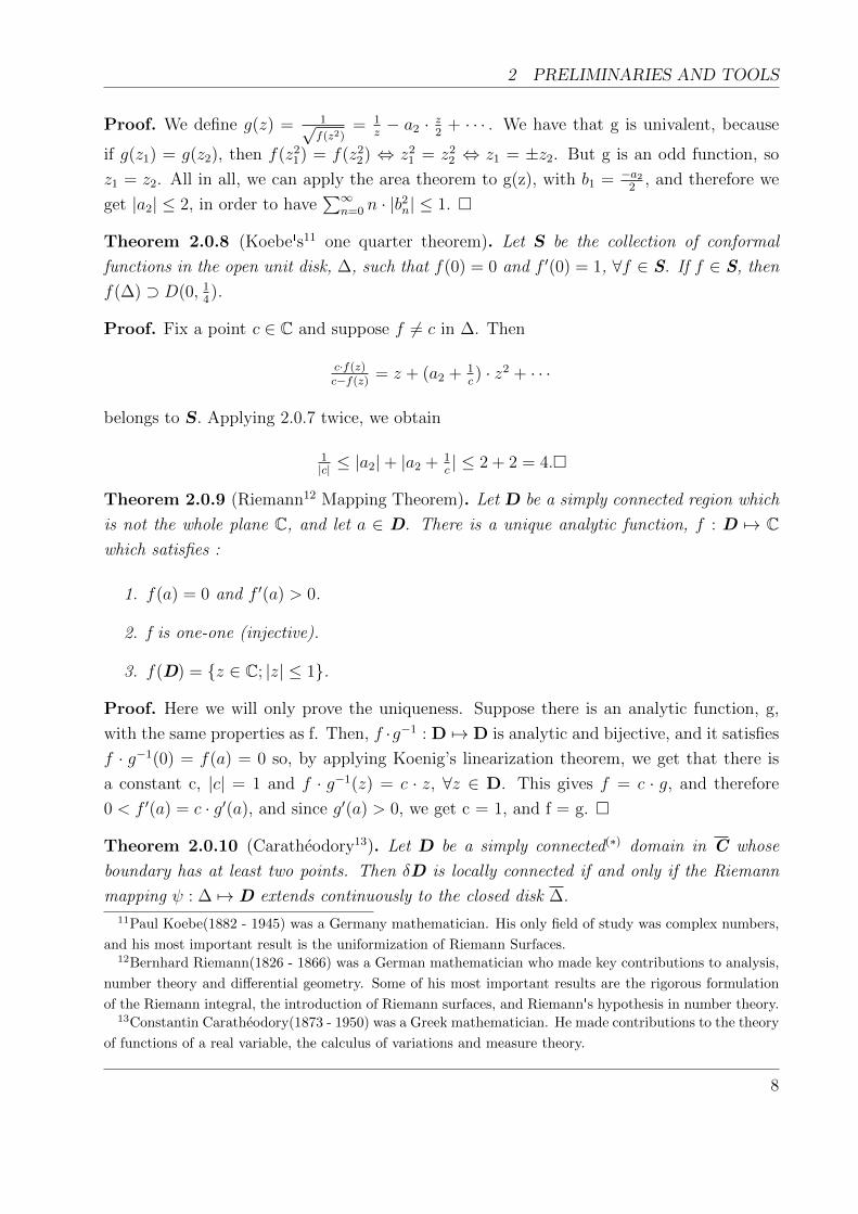
Theorem 2.0.8 (Koebe's11 one quarter theorem). Let S be the collection of conformal
functions in the open unit disk, ∆, such that f(0) = 0 and f ′(0) = 1, ∀f ∈ S. If f ∈ S, then
f(∆) ⊃ D(0, 14).
Proof. Fix a point c ∈ C and suppose f 6= c in ∆. Then
c·f(z)c−f(z) = z + (a2 + 1
c) · z2 + · · ·
belongs to S. Applying 2.0.7 twice, we obtain
1|c| ≤ |a2|+ |a2 + 1
c| ≤ 2 + 2 = 4.
Theorem 2.0.9 (Riemann12 Mapping Theorem). Let D be a simply connected region which
is not the whole plane C, and let a ∈ D. There is a unique analytic function, f : D 7→ Cwhich satisfies :
1. f(a) = 0 and f ′(a) > 0.
2. f is one-one (injective).
3. f(D) = z ∈ C; |z| ≤ 1.
Proof. Here we will only prove the uniqueness. Suppose there is an analytic function, g,
with the same properties as f. Then, f ·g−1 : D 7→ D is analytic and bijective, and it satisfies
f · g−1(0) = f(a) = 0 so, by applying Koenig’s linearization theorem, we get that there is
a constant c, |c| = 1 and f · g−1(z) = c · z, ∀z ∈ D. This gives f = c · g, and therefore
0 < f ′(a) = c · g′(a), and since g′(a) > 0, we get c = 1, and f = g.
Theorem 2.0.10 (Caratheodory13). Let D be a simply connected(∗) domain in C whose
boundary has at least two points. Then δD is locally connected if and only if the Riemann
mapping ψ : ∆ 7→ D extends continuously to the closed disk ∆.
11Paul Koebe(1882 - 1945) was a Germany mathematician. His only field of study was complex numbers,
and his most important result is the uniformization of Riemann Surfaces.12Bernhard Riemann(1826 - 1866) was a German mathematician who made key contributions to analysis,
number theory and differential geometry. Some of his most important results are the rigorous formulation
of the Riemann integral, the introduction of Riemann surfaces, and Riemann's hypothesis in number theory.13Constantin Caratheodory(1873 - 1950) was a Greek mathematician. He made contributions to the theory
of functions of a real variable, the calculus of variations and measure theory.
8
2 PRELIMINARIES AND TOOLS
Proposition 2.0.11. A conformal mapping of ∆ on to itself has the form
w = ei·θ · (z−a)(1−a·z) , 0 ≤ θ ≤ 2π, |a| < 1
Theorem 2.0.12. Every conformal automorphism, g, of C can be expressed as a Mobius
transformation(∗)
g(z) = a·z+bc·z+d
where a, b, c, d ∈ C, and ad− bc 6= 0. Every non-identity automorphism of C either has two
distinct fixed points or one double fixed point in C.
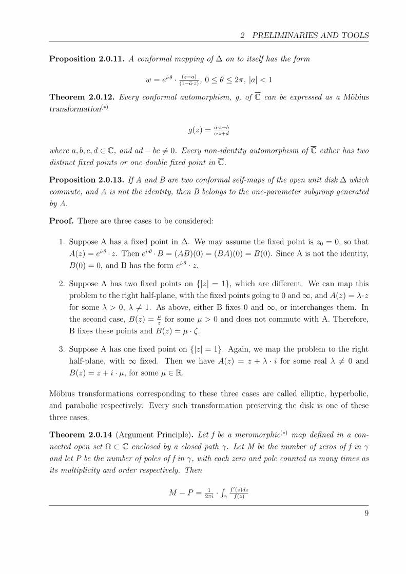
Proposition 2.0.13. If A and B are two conformal self-maps of the open unit disk ∆ which
commute, and A is not the identity, then B belongs to the one-parameter subgroup generated
by A.
Proof. There are three cases to be considered:
1. Suppose A has a fixed point in ∆. We may assume the fixed point is z0 = 0, so that
A(z) = ei·θ · z. Then ei·θ ·B = (AB)(0) = (BA)(0) = B(0). Since A is not the identity,
B(0) = 0, and B has the form ei·θ · z.
2. Suppose A has two fixed points on |z| = 1, which are different. We can map this
problem to the right half-plane, with the fixed points going to 0 and∞, and A(z) = λ·zfor some λ > 0, λ 6= 1. As above, either B fixes 0 and ∞, or interchanges them. In
the second case, B(z) = µz
for some µ > 0 and does not commute with A. Therefore,
B fixes these points and B(z) = µ · ζ.
3. Suppose A has one fixed point on |z| = 1. Again, we map the problem to the right
half-plane, with ∞ fixed. Then we have A(z) = z + λ · i for some real λ 6= 0 and
B(z) = z + i · µ, for some µ ∈ R.
Mobius transformations corresponding to these three cases are called elliptic, hyperbolic,
and parabolic respectively. Every such transformation preserving the disk is one of these
three cases.
Theorem 2.0.14 (Argument Principle). Let f be a meromorphic(∗) map defined in a con-
nected open set Ω ⊂ C enclosed by a closed path γ. Let M be the number of zeros of f in γ
and let P be the number of poles of f in γ, with each zero and pole counted as many times as
its multiplicity and order respectively. Then
M − P = 12πi·∫γf ′(z)dzf(z)
9
2 PRELIMINARIES AND TOOLS
Now we will consider hyperbolic metric, which is very important in complex dynamics, as
every holomorphic function is a contraction with respect to this metric (this result is known
as the Schwarz-Pick lemma).
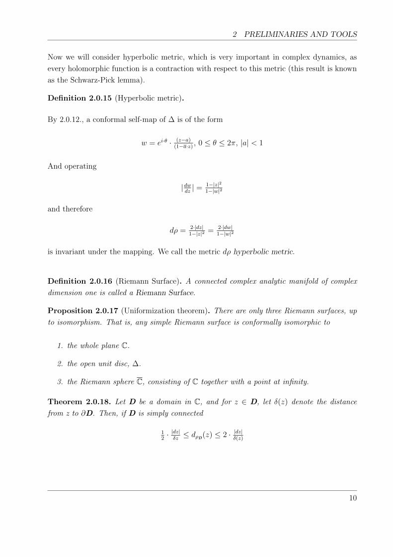
Definition 2.0.15 (Hyperbolic metric).
By 2.0.12., a conformal self-map of ∆ is of the form
w = ei·θ · (z−a)(1−a·z) , 0 ≤ θ ≤ 2π, |a| < 1
And operating
|dwdz| = 1−|z|2
1−|w|2
and therefore
dρ = 2·|dz|1−|z|2 = 2·|dw|
1−|w|2
is invariant under the mapping. We call the metric dρ hyperbolic metric.
Definition 2.0.16 (Riemann Surface). A connected complex analytic manifold of complex
dimension one is called a Riemann Surface.
Proposition 2.0.17 (Uniformization theorem). There are only three Riemann surfaces, up
to isomorphism. That is, any simple Riemann surface is conformally isomorphic to
1. the whole plane C.
2. the open unit disc, ∆.
3. the Riemann sphere C, consisting of C together with a point at infinity.
Theorem 2.0.18. Let D be a domain in C, and for z ∈ D, let δ(z) denote the distance
from z to ∂D. Then, if D is simply connected
12· |dz|δz≤ dρD(z) ≤ 2 · |dz|
δ(z)
10

3 INTRODUCTION AND LOCAL THEORY
3 INTRODUCTION AND LOCAL THEORY
3.1 INTRODUCTORY RESULTS
Given a continuous function f : C 7→ C, the set of all the iterates, fn(z0), n ≥ 0, for the
various points z0 ∈ C is a dynamical system where a ”force”, f, for each period, n, changes
z0 into fn(z0). From this point of view, the main question is where will z0 be when iterated
by f many times. Mathematically, our aim is to study the asymptotic behavior of fn(z0)
when n 7→ ∞ for every z0 ∈ C. In this same line of thinking we may also ask ourselves about
the previous states of a given point; Due to the nature of functions, the question about the
future states of an initial seed is uniquely determined (that is, if we can find the solution),
but, on the other hand, the question about the previous states of a point does not have, in
general, a unique answer, unless the map, f, is globally invertible.
To accomplish our goal we first characterize some types of points which have a special
behavior and characteristics:
Definition 3.1.1 (Fixed point). An element z ∈ C is said to be a fixed point of f : C 7→ Cif f(z) = z.
Definition 3.1.2 (Periodic point). An element z ∈ C is said to be a periodic point of period
p of f if fp(z) = z and fn(z) 6= z, ∀n < p, n, p ∈ N. In this case, the orbit of z0, called
periodic orbit, is given by the finite set z0, z1, . . . , zp−1.
There is a strong relation between the fixed points of fp and the periodic points of f: a fixed
point of fp is either a fixed point of f, or a periodic point of period d of f, for some d|p.
Definition 3.1.3 (Preperiodic point). An element z ∈ C is said to be a preperiodic point of
f if z is not periodic, but a point in its orbit is periodic.
We have only considered two types of special orbits, but, taking benefit from the special
nature of periodic points, we can determine, in some cases, how will nearby points (points
in a neighborhood of the periodic point) behave when iterated by the same function f.
Definition 3.1.4 (Classification of fixed points). Given a fixed a point, z0, of an holomorphic
function f, we call λ = f ′(z0) its multiplier. We can classify the fixed point according to λ:
1. if |λ| < 1, the fixed point is attracting (if λ = 0, we say the fixed point is superattract-
ing).
11

3 INTRODUCTION AND LOCAL THEORY
2. if |λ| > 1, the fixed point is repelling.
3. if |λ| = 1 and λn = 1, for some n ∈ Z, the fixed point is rationally neutral.
4. if |λ| = 1 and λn 6= 1, for every n ∈ Z, the fixed point is irrationally neutral.
As its name states, an attracting point is a fixed point that attracts nearby points when
they are iterated by f. Indeed, if |λ| < ρ < 1 then, in a neighborhood of z0, |f(z) − z0| <ρ · |z − z0| ⇒ |fn(z) − z0| < ρn · |z − z0| and therefore fn(z) uniformly converges(∗) to z0
on such neighborhood; this concept opposes to that of a repelling fixed point. In the case
of |λ| = 1, the nature of the fixed point is not as obvious, and requires a further study to
determine the behavior of nearby points.
Definition 3.1.5 (Basin of attraction). Given an attracting fixed point z0 ∈ C, we define its
basin of attraction as A(z0) = z ∈ C such that fn is defined for all n ≥ 1 and fn(z)→ z0,
when n→∞ , where fn is the n-fold iterate of f.
Observation. A(z0) is open, because it is the union of the backwards iterates f−n(D(z0, ε)),
for a given small ε > 0.
Definition 3.1.6 (Classification of periodic points). Given a periodic orbit z0z1 . . . zp−1for the function f, we may see z0 as a fixed point of g(z) = fp(z), and therefore we define
the multiplier of the periodic orbit
g′(z0) =∏i=p−1
i=0 f ′(zi)
which determines its local nature.
The same results given for a fixed point stand true for a periodic orbit, using the new concept
of multiplier that we have just defined. Therefore, periodic orbits can be classified the same
way as fixed points.
3.2 LOCAL THEORY
In some cases, it might be difficult to determine the basin of attraction of an attracting fixed
point for a given function, or the dynamics of points in a neighborhood of periodic points.
To solve this problem, we can sometimes use other simpler functions that we already know
the behavior of, and obtain results of the original functions from them. We do this by using
conjugations.
12
3 INTRODUCTION AND LOCAL THEORY
Definition 3.2.1 (Conformal conjugations). We say that a function f : U ⊂ C 7−→ U is
conformally conjugate to g : V ⊂ C 7−→ V if there is a conformal map(∗) φ : U 7−→ V such
that
φ(f(z)) = g(φ(z)),∀z ∈ U
We may consider f and g to be the same map expressed in different coordinates. Note that φ
maps fixed points to fixed points, and the multipliers associated to those fixed points remain
equal by φ. It also maps a basin of attraction by f to a basin of attraction by g.
This definition also implies that the iterates fn and gn are also conjugated by φ, i.e :
gn = φ · fn · φ−1.
We have only defined, and will only be considering, conformal conjugations. However, there
are also other types of conjugations: if instead of considering a conformal map φ : U 7→ V
conjugating f and g, we consider a map φ : U 7→ V which is continuous (C1) we get a
continuous (C1) conjugation.
These other conjugations also map fixed points to fixed points, periodic orbits to periodic
orbits, . . . . However, the difference between them and a conformal conjugation is that the
latter does not alter the multiplier of the periodic orbits.
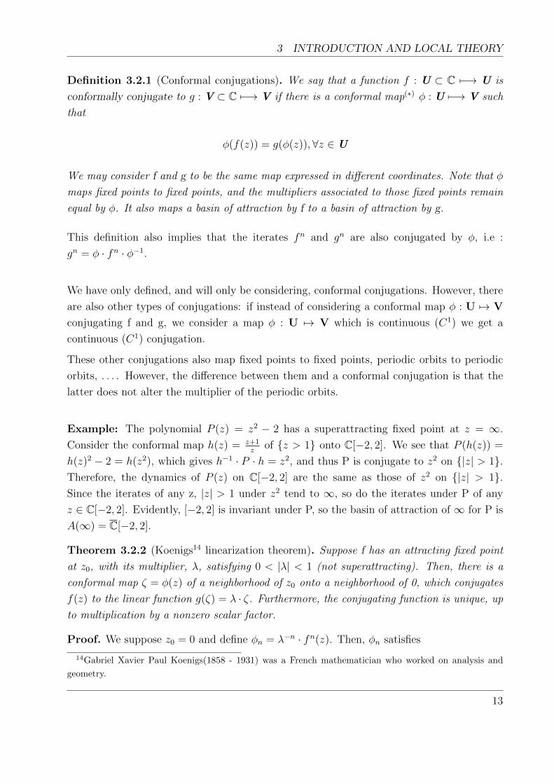
Example: The polynomial P (z) = z2 − 2 has a superattracting fixed point at z = ∞.
Consider the conformal map h(z) = z+1z
of z > 1 onto C[−2, 2]. We see that P (h(z)) =
h(z)2 − 2 = h(z2), which gives h−1 · P · h = z2, and thus P is conjugate to z2 on |z| > 1.Therefore, the dynamics of P (z) on C[−2, 2] are the same as those of z2 on |z| > 1.Since the iterates of any z, |z| > 1 under z2 tend to ∞, so do the iterates under P of any
z ∈ C[−2, 2]. Evidently, [−2, 2] is invariant under P, so the basin of attraction of ∞ for P is
A(∞) = C[−2, 2].
Theorem 3.2.2 (Koenigs14 linearization theorem). Suppose f has an attracting fixed point
at z0, with its multiplier, λ, satisfying 0 < |λ| < 1 (not superattracting). Then, there is a
conformal map ζ = φ(z) of a neighborhood of z0 onto a neighborhood of 0, which conjugates
f(z) to the linear function g(ζ) = λ · ζ. Furthermore, the conjugating function is unique, up
to multiplication by a nonzero scalar factor.
Proof. We suppose z0 = 0 and define φn = λ−n · fn(z). Then, φn satisfies
14Gabriel Xavier Paul Koenigs(1858 - 1931) was a French mathematician who worked on analysis and
geometry.
13

3 INTRODUCTION AND LOCAL THEORY
φn · f = λ−n · fn+1 = λ · φn+1
Therefore, if φn 7→ φ, then φ · f = λ · φ, so φ · f · φ−1 = λ · ζ ⇒ φ is a conjugation. To show
convergence note that for δ > 0 small,
|f(z)− λ · z| ≤ C · |z|2, |z| ≤ δ
Thus |f(z)| ≤ |λ| · |z|+ C · |z|2 ≤ (|λ|+ C · δ) · |z| and, by induction, with |λ|+ C · δ < 1,
|fn(z)| ≤ (|λ|+ C · δ)n · |z|, |z| ≤ δ
We choose δ > 0 so small that ρ = (|λ|+C·δ)2|λ| < 1, and we obtain
|φn+1(z)− φn(z)| = |fn(f(z))−λ·fn(z)
λn+1 | ≤ C·|fn(z)|2|λ|n+1 ≤ ρn·C·|z|2
|λ|
for |z| ≤ δ. Therefore φn(z) converges uniformly for |z| ≤ δ, and the conjugation exists.
Now we will prove the uniqueness:
Suppose there are two such conjugations, φ1 and φ2. Then, the composition
φ2 · φ−11 (z) = a1 · z + a2 · z2 + . . . , for some ai ∈ C, i ∈ N
would commute with the map s(z) = λ ·z, and comparing the coefficients of the two resulting
power series we get λ · an = an · λn, ∀n ∈ N. Since λ is not zero nor a root of the unity,
a2 = a3 = · · · = 0, and therefore φ2 · φ−11 (z) = a1 · z, or equivalently φ2 = a1 · φ1.
Proposition 3.2.3 (The repelling case). The existence of a conjugating map for a repelling
fixed point follows from the attracting case, because if f(z0) = z0, f ′(z0) = λ > 1, we know
that f ′(z) 6= 0, ∀z ∈ U, where U is a neighborhood of z0. Therefore, there is a branch of
f−1, g(z), in U for which z0 is a fixed point. Applying the inverse function theorem, we
know that g′(z0) = 1λ
= µ, µ < 1, and there is a conformal conjugation ζ = φ(z) such that
ζg(z) = µ · ζ = ζλ
And this same map also conjugates f(z) to λ · ζ.
In the case of superattracting fixed points we can also prove the existence of a conjugation.
Proposition 3.2.4 (Bottcher15 coordinates). Suppose f has a superattracting fixed point at
z015Lucjan Bottcher(1872 - 1937) was a Polish mathematician. His most important result was in the iteration
of rational mappings of the Riemann sphere.
14
3 INTRODUCTION AND LOCAL THEORY
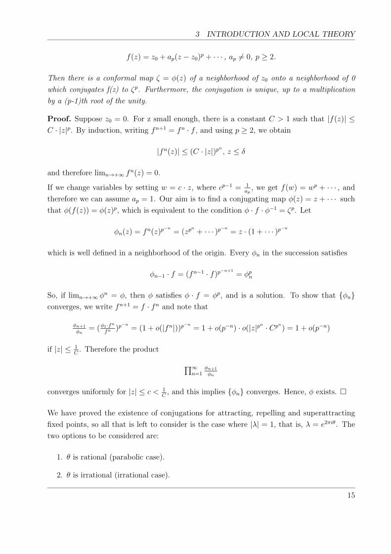
f(z) = z0 + ap(z − z0)p + · · · , ap 6= 0, p ≥ 2.
Then there is a conformal map ζ = φ(z) of a neighborhood of z0 onto a neighborhood of 0
which conjugates f(z) to ζp. Furthermore, the conjugation is unique, up to a multiplication
by a (p-1)th root of the unity.
Proof. Suppose z0 = 0. For z small enough, there is a constant C > 1 such that |f(z)| ≤C · |z|p. By induction, writing fn+1 = fn · f , and using p ≥ 2, we obtain
|fn(z)| ≤ (C · |z|)pn , z ≤ δ
and therefore limn→+∞ fn(z) = 0.
If we change variables by setting w = c · z, where cp−1 = 1ap
, we get f(w) = wp + · · · , and
therefore we can assume ap = 1. Our aim is to find a conjugating map φ(z) = z + · · · such
that φ(f(z)) = φ(z)p, which is equivalent to the condition φ · f · φ−1 = ζp. Let
φn(z) = fn(z)p−n
= (zpn
+ · · · )p−n = z · (1 + · · · )p−n
which is well defined in a neighborhood of the origin. Every φn in the succession satisfies
φn−1 · f = (fn−1 · f)p−n+1
= φpn
So, if limn→+∞ φn = φ, then φ satisfies φ · f = φp, and is a solution. To show that φn
converges, we write fn+1 = f · fn and note that
φn+1
φn= (φ1·f
n
fn)p−n
= (1 + o(|fn|))p−n = 1 + o(p−n) · o(|z|pn · Cpn) = 1 + o(p−n)
if |z| ≤ 1C
. Therefore the product
∏∞n=1
φn+1
φn
converges uniformly for |z| ≤ c < 1C
, and this implies φn converges. Hence, φ exists.
We have proved the existence of conjugations for attracting, repelling and superattracting
fixed points, so all that is left to consider is the case where |λ| = 1, that is, λ = e2πiθ. The
two options to be considered are:
1. θ is rational (parabolic case).
2. θ is irrational (irrational case).
15
3 INTRODUCTION AND LOCAL THEORY
Suppose λ = e2πiθ, with θ rational. As θ is rational, θ = pq, for some p, q ∈ Z, we may
consider f q, which satisfies λ = 1, because if φ is a conformal conjugation between f and g,
it is also a conformal conjugation of f q and gq.
Definition 3.2.5 (Order or multiplicity of a fixed point). The order of z0 as a fixed point
of f : U 7→ C is the order or multiplicity of z0 as a zero of f(z) − z, that is, the degree
of the first non-vanishing term of the Taylor 's expansion of f - Id at z0(in any set of local
coordinates centered at z0).
Considering the Taylor's expansion, we therefore take maps of the form
f(z) = z + a · zm+1 + o(zm+2), m > 0 and a 6= 0
where m is the order of z0.
Definition 3.2.6 (Attracting and repelling petals). Suppose f is defined and univalent in a
neighborhood, U, of the origin. An open set P ⊂ U is called an attracting petal for f at the
fixed point if
1. f(P) ⊂ P ∪ 0.
2.⋂n f
n(P) = 0.
An open set P ⊂ U is called a repelling petal for f at the fixed point if P is an attracting
point for f−1 : f(U) 7→ U, where f−1 denotes the branch of the inverse of f fixing the origin.
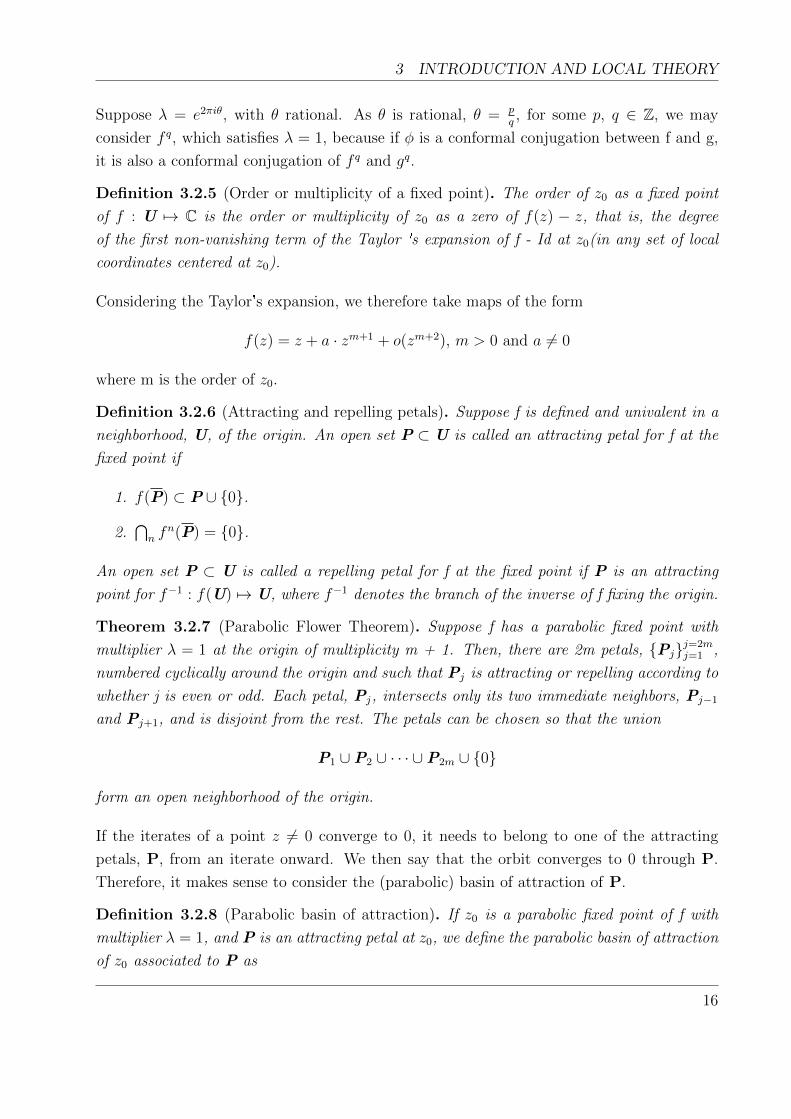
Theorem 3.2.7 (Parabolic Flower Theorem). Suppose f has a parabolic fixed point with
multiplier λ = 1 at the origin of multiplicity m + 1. Then, there are 2m petals, Pjj=2mj=1 ,
numbered cyclically around the origin and such that Pj is attracting or repelling according to
whether j is even or odd. Each petal, Pj, intersects only its two immediate neighbors, Pj−1
and Pj+1, and is disjoint from the rest. The petals can be chosen so that the union
P1 ∪P2 ∪ · · · ∪P2m ∪ 0
form an open neighborhood of the origin.
If the iterates of a point z 6= 0 converge to 0, it needs to belong to one of the attracting
petals, P, from an iterate onward. We then say that the orbit converges to 0 through P.
Therefore, it makes sense to consider the (parabolic) basin of attraction of P.
Definition 3.2.8 (Parabolic basin of attraction). If z0 is a parabolic fixed point of f with
multiplier λ = 1, and P is an attracting petal at z0, we define the parabolic basin of attraction
of z0 associated to P as
16

3 INTRODUCTION AND LOCAL THEORY
Figure 1: Distribution of the invariant petals around a parabolic point with multiplicity 5.
Figure 2: Distribution of the invariant petals around a parabolic point with multiplicity 3.
17

3 INTRODUCTION AND LOCAL THEORY
Ap = z ∈ S \⋃n>0 f
−n(z0)|fn(z) 7→ z0 through P when n 7→ ∞
If the parabolic point has multiplicity m + 1, then it has exactly m disjoint parabolic basins.
Although we can not find a conjugation to its linear part as we have for attracting, repelling
and superattracting fixed points, some kind of linearization is possible inside each petal.
Theorem 3.2.9 (Fatou16 Coordinates). For every attracting and for every repelling petal
P, there is a conformal embedding
φ : P 7→ C
mapping 0 to ∞, called the Fatou coordinate in P, which conjugates f to the translation
z 7→ z + 1 on P ∩ f−1(P ).
Consider now the case where λ = e2πiθ, with θ irrational. Our aim is to find a solution to
the Schroder17 equation φ(f(z)) = λφ(z), normalized by φ′(0) = 1. If we write h = φ−1, the
equation becomes
f(h(ζ)) = h(λ · ζ), h′(0) = 1
Theorem 3.2.10 (Uniqueness of solutions). A solution to the Schroder equation in any disk
|ζ| > r is unique.
Proof. Suppose h(ζ1) = h(ζ2) ⇒ h(λn · ζ1) = h(λn · ζ2) for all n > 0, n ∈ N. Since λn is
dense in the unit circle (as θ is irrational), h(ζ1 · ei·θ) = h(ζ2 · ei·θ) for every θ. This implies
h(ζ1 · z) = h(ζ2 · z) for |z| < 1, and since h′(0) = 1, ζ1 = ζ2.
Theorem 3.2.11 (Existence of solution ). A solution h of the Schroder equation exists if
and only if the sequence of iterates fn is uniformly bounded in some neighborhood of the
origin.
Proof. If h exists, then fn(z) = h(λn · h−1(z)) is obviously bounded. On the other hand, if
|fn(z)| ≤M , for some M ∈ R and ∀n ≥ 1, we can define:
φn(z) = 1n
∑j=n−1j=0 λ−j · f j(z)
16Pierre Fatou(1878 - 1929) was a French mathematician and astronomer. He made important contribu-
tions to the field of analysis. As seen in this project later, he gives name to the Fatou Set.17Ernst Schroder(1841 - 1902) was a German mathematician, mostly known by his work in algebraic logic.
18
3 INTRODUCTION AND LOCAL THEORY
Then φn is a uniformly bounded sequence of analytic functions, and therefore contains a
convergent subsequence. Since φn · f = λ · φn + o( 1n), any limit of the sequence φn satisfies
φ · f = λ · φ. From λ = f ′(0), we get φ′n(0) = 1 and so φ′(0) = 1. All in all, h = φ−1 is a
solution of the Schroder equation.
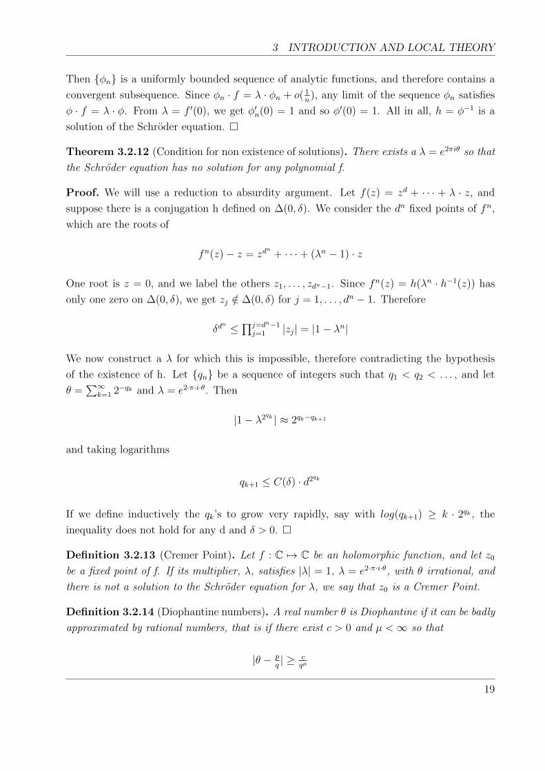
Theorem 3.2.12 (Condition for non existence of solutions). There exists a λ = e2πiθ so that
the Schroder equation has no solution for any polynomial f.
Proof. We will use a reduction to absurdity argument. Let f(z) = zd + · · · + λ · z, and
suppose there is a conjugation h defined on ∆(0, δ). We consider the dn fixed points of fn,
which are the roots of
fn(z)− z = zdn
+ · · ·+ (λn − 1) · z
One root is z = 0, and we label the others z1, . . . , zdn−1. Since fn(z) = h(λn · h−1(z)) has
only one zero on ∆(0, δ), we get zj /∈ ∆(0, δ) for j = 1, . . . , dn − 1. Therefore
δdn ≤
∏j=dn−1j=1 |zj| = |1− λn|
We now construct a λ for which this is impossible, therefore contradicting the hypothesis
of the existence of h. Let qn be a sequence of integers such that q1 < q2 < . . . , and let
θ =∑∞
k=1 2−qk and λ = e2·π·i·θ. Then
|1− λ2qk | ≈ 2qk−qk+1
and taking logarithms
qk+1 ≤ C(δ) · d2qk
If we define inductively the qk’s to grow very rapidly, say with log(qk+1) ≥ k · 2qk , the
inequality does not hold for any d and δ > 0.
Definition 3.2.13 (Cremer Point). Let f : C 7→ C be an holomorphic function, and let z0
be a fixed point of f. If its multiplier, λ, satisfies |λ| = 1, λ = e2·π·i·θ, with θ irrational, and
there is not a solution to the Schroder equation for λ, we say that z0 is a Cremer Point.
Definition 3.2.14 (Diophantine numbers). A real number θ is Diophantine if it can be badly
approximated by rational numbers, that is if there exist c > 0 and µ <∞ so that
|θ − pq| ≥ c
qµ
19

3 INTRODUCTION AND LOCAL THEORY
If we write λ = e2πiθ, this condition is equivalent to
|λn − 1| ≥ c · n1−µ, n ≥ 1
Proposition 3.2.15 (Existence of Diophantine numbers). For a fixed µ > 2, the condition
|θ − pq| ≥ c
qµholds for almost every real number θ. Indeed, if E is the set of θ ∈ [0, 1], such
that |θ − pq| < 1
qµinfinitely often, then
|E| ≤∑∞
q=n 2 · q−µ · q = o(n2−µ) 7→ 0
In particular, almost all real numbers are Diophantine.
The first theorem about the existence of linearizable points is due to Siegel, and it was an
important breakthrough at the time. Since then, the conditions used by Siegel have been
improved by other mathematicians such as Herman18 or Bruno19. We conclude this section
by stating Siegel's original theorem.
Theorem 3.2.16 (Siegel20). If θ is Diophantine, and if f has a fixed point at 0 with multiplier
e2πiθ, then there is a solution to the Schroder equation. In other words, f can be conjugated
near 0 to multiplication by e2πiθ.
18Michael Herman(1942 - 2000) was a French-American mathematician. He was one of the most known
figures in dynamical systems. One of his most important results was the introduction of Herman Rings in
1979.19Alexander Bruno(1940) is a Russian mathematician who has made contributions to the normal forms
theory.20Carl Ludwig Siegel(1896 - 1981) was a German mathematician. His main field of work was number theory
and celestial mechanics. His most known results are his contribution to the Thue-Siegel-Roth theorem for
Diophantine approximation and the Siegel Mass Formula for quadratic forms. He is considered one of the
most important mathematicians in the XX century.
20

4 GLOBAL THEORY
4 GLOBAL THEORY
We will now study the phase space of holomorphic functions as a whole, not just locally, so
we can determine the behavior of points anywhere on the plane.
4.1 GENERAL RESULTS
Definition 4.1.1 (Fatou and Julia21 Set). Let S be a Riemann surface, f : S 7→ S a non-
constant holomorphic mapping, and let fn : S 7→ S be its n-fold iterate. Given a fixed z0 ∈ S,
if there exists a neighborhood of z0, U, so that the sequence of iterates fnn restricted to U
forms a normal family, then we say that z0 is a normal point, or that it belongs to the Fatou
Set of f. On the other hand, if such neighborhood does not exist, we say that z0 belongs to
the Julia Set of f.
Therefore, by definition, the Julia Set is a closed set and the Fatou Set is open. We may
think of the Fatou Set as the set or orbits which are in some sense stable, and the Julia Set
as the set of chaotic orbits.
Example: Consider the map f : C 7→ C, f(z) = z2. The entire open disk, ∆, is contained
in the Fatou Set of f, since successive iterates on any compact subset converge uniformly
to zero. Likewise, the set C \ ∆ is contained in the Fatou Set of f, since the iterates of f
converge to ∞. On the other hand, if z0 is a point of the unit circle, in any neighborhood of
this point, any limit of iterates would have a jump discontinuity as we cross the unit circle.
This shows that J = S1.
However, not all Julia Sets are as easy to compute and draw as this one. The next example
shows a more complicated Julia Set:
Example: Consider the map f : C 7→ C, f(z) = z2−1. In this case, f has two repelling fixed
points, z± = 1±√5
2and an attracting two cycle : 0,−1 (actually, it is a superattracting
cycle). The Julia Set corresponding to this map is actually a fractal, and it has infinitely
many connected components.
We present some properties of both sets to further characterize them.
21Gaston Julia(1893 - 1978) was a French mathematician who devised the formula for the Julia Set. His
work gained a lot of popularity with the use of the computer for mathematical research, as it could then be
visualized.
21
4 GLOBAL THEORY
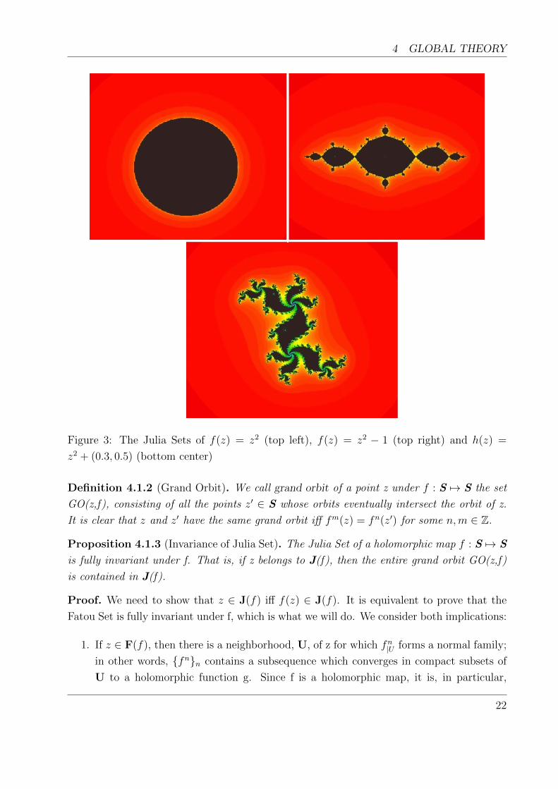
Figure 3: The Julia Sets of f(z) = z2 (top left), f(z) = z2 − 1 (top right) and h(z) =
z2 + (0.3, 0.5) (bottom center)
Definition 4.1.2 (Grand Orbit). We call grand orbit of a point z under f : S 7→ S the set
GO(z,f), consisting of all the points z′ ∈ S whose orbits eventually intersect the orbit of z.
It is clear that z and z′ have the same grand orbit iff fm(z) = fn(z′) for some n,m ∈ Z.
Proposition 4.1.3 (Invariance of Julia Set). The Julia Set of a holomorphic map f : S 7→ S
is fully invariant under f. That is, if z belongs to J(f), then the entire grand orbit GO(z,f)
is contained in J(f).
Proof. We need to show that z ∈ J(f) iff f(z) ∈ J(f). It is equivalent to prove that the
Fatou Set is fully invariant under f, which is what we will do. We consider both implications:
1. If z ∈ F(f), then there is a neighborhood, U, of z for which fn|U forms a normal family;
in other words, fnn contains a subsequence which converges in compact subsets of
U to a holomorphic function g. Since f is a holomorphic map, it is, in particular,
22

4 GLOBAL THEORY
open and therefore f(U) is an open neighborhood of f(z). If we consider fn|f(U), it is
also normal, because f(f(z)) = f 2(z), f 2(f(z)) = f 3(z), etc... And therefore if fnk
converges in compact subsets of U to g, then fnk−1 converges in compact subsets of
f(U), and is therefore normal in f(U). All in all, f(z) ∈ F(f).
2. Let u ∈ S such that f(u) = z, and u ∈ F(f). We want to see that z ∈ F(f). Again,
because f is holomorphic, it is in particular continuous, and therefore f−1(U) is an open
neighborhood of u. As above, we see that f 2(z) = f 3(f−1(z)), f 3(z) = f 4(f−1(z)), etc...
Therefore, if fnk+1 converges in compact subsets of f−1(U) to g, then fnk converges in
compact subsets of U, and is therefore normal in U. All in all, z ∈ F(f).
Proposition 4.1.4. For any n > 0, n ∈ N, the set J(fn) = J(f).
Proof. Again, it is equivalent to prove that F(fn) = F(f). We will prove both inclusions:
1. Suppose z ∈ F(f) and we want to see that z ∈ F(fn). If z ∈ F(f), there is a
neighborhood, U, such that fp|U is normal, that is fpk contains a subsequence which
converges in compact subsets of U to a holomorphic function g. But, since every
subsequence of fpnk is also a subsequence of fpk , the result is clear.
2. Suppose z ∈ F(fn) and we want to see that z ∈ F(f). We know that if fp is normal,
then fp+j is also normal, for every j ∈ N(we have seen this in the previous theorem).
We can express
fp =⋃rf rp ∪ f rp+1 ∪ ... ∪ f rp+(r−1)
so any partial of fpmust contain infinite terms of the form f rp, f rp+1, ..., or f rp+(r−1),
as it can not have finitely many of all of them. Therefore, if a subsequence of fnp is
convergent, there is also a convergent subsequence of fp, which is what we wanted to
prove.
Theorem 4.1.5 (Periodic orbits and Fatou Set). Every attracting, periodic orbit of a map
is contained in its Fatou Set. In fact, the whole basin of attraction, Ω, of that periodic orbit
is contained in the Fatou Set. However, its boundary, ∂Ω is contained in the Julia Set, as is
every repelling orbit.
Proof. We only need to consider the case of a fixed point, f(z0) = z0, as the previous
proposition states that J(fn) = J(f), for every n > 0, n ∈ N (in this particular case we take
n to be the period of the orbit). If z0 is attracting, it follows from Taylor’s Theorem that
the successive iterates of f , restricted to a neighborhood of z0, converge uniformly to the
constant function
23
4 GLOBAL THEORY
g : S 7→ S
z 7→ z0
We can apply this to any compact subset of the basin of attraction, Ω. On the other hand,
if z ∈ Ω, but z /∈ Ω, it is clear that no sequence of iterates can converge to a continuous
limit. Finally, if z0 is repelling, then no sequence of iterates can converge uniformly near z0,
since the derivative dfn(z)dz
takes the value λn (with λ > 1) and therefore diverges to infinity
as n 7→ ∞.
Theorem 4.1.6. If z0 ∈ J(f), then the set of all iterated pre-images
A = z : fn(z) = z0 for some n ≥ 0, n ∈ N
is everywhere dense in J(f). In particular, it follows that the corresponding grand orbit,
GO(z0,f) is everywhere dense in J(f).
This theorem is specially important, as it gives us an effective way of computing images of
Julia Sets: starting with any z0 ∈ J(f), we compute all pre-images of such point, that is,
A = z1 ∈ C such that f(z1) = z0; then we compute all the pre-images of the points in A,
and so on. Eventually, we will be coming arbitrarily close to every point of J(f).
Corollary 4.1.7. For generic(∗) z ∈ J(f), the forward orbit
z, f(z), f 2(z), · · ·
is everywhere dense in J(f).
Proof. Let Bjn be a countable collection of open sets forming a basis for the topology of
C. For each Bj which intersects J(f), let Uj be the union of the iterated pre-images f−n(Bj)
for n ≥ 0, n ∈ N. Then it follows from the previous theorem that the closure of Uj ∩ J(f)
is equal to the entire Julia Set, J(f), and the conclusion follows.
The results given up to this point are valid for any function. From here we will focus on
rational functions and give a deeper characterization of them.
4.2 RATIONAL FUNCTIONS
Let R(z) be rational, R = PQ
, where P and Q are polynomials with no common factors and
d = max(degP, degQ) ≥ 2.
24
4 GLOBAL THEORY
Theorem 4.2.1. The Julia Set is nonempty.
Proof. Suppose J = ∅. Then, Rn is a normal family on all of C, and so there is a
subsequence nk, k ∈ N, such that Rnk 7→ f(z) for some analytic function f : C 7→ C. Since
f is analytic on all of C, it is a rational function, as it can not have infinitely many poles and
zeros. If f is constant, the image of Rnk is eventually contained in a small neighborhood of
the constant value, which is impossible since Rnk covers C. If f is not constant, eventually
Rnk has the same number of zeros as f(this follows from the argument principle), which is
also impossible, since the number of zeros of Rn grows monotonically.
Theorem 4.2.2. The Julia Set, J, contains no isolated points, that is, J is a perfect set.
Proof. Take z0 ∈ J and U an open neighborhood of z0. First assume z0 is not periodic and
choose z1 with R(z1) = z0. Then R(z0) 6= z1 for all n. Since z1 ∈ J, backward iterates of z1
are dense in J, so there is a ζ ∈ U with Rm(ζ) = z1. Thus ζ ∈ J ∩U and ζ 6= z0.
Next, suppose Rn(z) = z0. Then z0 would be a superattracting fixed point for Rn, con-
tradicting z0 ∈ J. Hence there is z1 6= z0 with Rn(z1) = z0. Furthermore Rj(z0) 6= z1
for all j, since otherwise it would hold for some 0 ≤ j < n (by periodicity) and therefore
Rj(z0) = Rn+j(z0) = Rn(z1) = z0, contradicting the minimality of n. As before, z1 must
have a preimage in U ∩ J which cannot be z0.
Theorem 4.2.3. The Julia Set of a rational map of degree d ≥ 2 is equal to the closure of
its set of periodic points.
Proof. We have just seen that J(f) has no isolated points, and therefore we can exclude
finitely many points of J(f) without affecting the argument. Let z0 be any point of J(f)
which is not a fixed point nor a critical value, that is, we assume that there are d preimages
z1, ..., zd which are distinct from each other and from z0, where d ≥ 2 is the degree of
f. By the Inverse Function Theorem, we can find d holomorphic functions, z 7→ φj(z),
0 ≤ j ≤ d− 1, which are defined throughout some neighborhood, V, of z0 and which satisfy
f(φj(z)) = z, with φj(z0) = zj. We claim that for some n > 0, n ∈ N, and for some z ∈ N,
the function fn(z) must take one of the three values z, φ1(z) or φ2(z). For otherwise, the
family of holomorphic functions
gn = (fn(z)−φ1(z))·(z−φ2(z))(fn(z)−φ2(z))·(z−φ1(z))
on V would avoid the three values 0, 1 and ∞, and therefore be a normal family. But this
is a contradiction, since then fn|V would also be normal, contradicting the hypothesis that
V intersects the Julia Set. Therefore, we can find z ∈ V so as to satisfy either fn(z) = z or
fn(z) = φj(z). Then, z is a periodic point of period n, or n + 1 respectively.
25

4 GLOBAL THEORY
This shows that every point in J(f) can be approximated arbitrarily close by periodic points.
We shall see later that all but finitely many points must repel, so, in fact, the Julia Set,
J(f), of a rational map of degree d ≥ 2 is equal to the close of its set of repelling periodic
points.
If R has an attracting fixed point z0, its basin of attraction, A(z0) is contained in the Fatou
Set. On the other hand, since the iterates of R do not converge to z0 on the complement of
A(z0), these iterates can not be normal on any open set meeting ∂A(z0).
Definition 4.2.4 (Siegel Disk). A simply connected component of the Fatou Set in which R
is conjugate to an irrational rotation is called a Siegel Disk.
Definition 4.2.5 (Herman Ring). A periodic component of period n, U, of the Fatou Set is
called a Herman Ring if it is doubly connected(∗) and Rn is conjugate to either a rotation on
an annulus or to a rotation followed by an inversion.
Theorem 4.2.6. The Julia Set contains all repelling periodic points and all neutral periodic
points which do not correspond to Siegel Disks. The Fatou Set contains all attracting periodic
points and all neutral periodic points corresponding to Siegel Disks.
Proof. As we have seen that F (f) = F (fn), we can assume without loss of generality that z0
is a fixed point, instead of a periodic point. If z0 is a neutral fixed point, by 3.2.11 we know
that fn is bounded in a neighborhood of z0 iff z0 ∈ F (f)( and in this case, z0 corresponds
to a Siegel disk). If instead z0 is a Cremer point, then there is not a solution to the Schroder
equation for λ, where λ is the multiplier of the periodic point z0, and therefore fn is not
bounded in a neighborhood of z0, hence z0 ∈ J(f).
If z0 is an attracting fixed point, fn is obviously bounded in a neighborhood of z0, and fn
contains a subsequence which converges uniformly to the constant function g(z) = z0(z0 ∈F (f)). If instead z0 is a repelling fixed point, |fn(z0)| 7→ ∞ when n 7→ ∞, and therefore no
limit function can exist for any subsequence(z0 ∈ J(f)).
4.2.1 FATOU COMPONENTS, NON-REPELLING CYCLES AND CRITI-
CAL POINTS
Here we will see the relation between the critical points of a map and its Fatou Set.
Definition 4.2.7 (Exceptional points). A point z ∈ C is called exceptional under a map f
if its grand orbit, GO(z, f) ⊂ C is a finite set.
26

4 GLOBAL THEORY
Proposition 4.2.8 (Number of exceptional points). If f is a rational map of degree two
or more, then the set E(f) of exceptional points can have, at most, two elements. These
exceptional points, if they exist, must be critical points of f, and they must belong to the
Fatou Set of f.
Proof. First we must notice that f maps any grand orbit onto itself, and therefore any finite
grand orbit must constitute a single periodic orbit under f. Each point in this orbit must
be critical, since otherwise f(z) would have two or more pre-images. We conclude then that
such an orbit must be superattracting, and therefore contained in the Fatou Set.
If there were three different grand orbit finite points, then the union of the grand orbits of
these points would form a finite set whose complement, U, in C would be hyperbolic, with
f(U) = U. By Montel's Theorem, the set of iterates of f restricted to U would be normal,
and therefore both U and its complement would be contained in the Fatou Set, contradicting
the previous theorem.
Proposition 4.2.9. If z0 is an attracting or parabolic periodic point, then the immediate
basin of attraction A∗(z0) contains at least one critical point.
Proof. If z0 is an attracting point, its multiplier, λ, satisfies 0 < |λ| < 1. Let U0 =
φ−1(∆(0, ε)) be a small disk, invariant under R, on which the analytic branch, f, of R−1
satisfying f(z0) = z0 is defined. The branch f maps U0 into A∗z0 and is one-to-one. Therefore,
U1 = f(U0) is simply connected, and U0 ⊂ U1, if U0 is appropriately chosen. If we do not
encounter any critical point, we keep on doing this process, constructing Un+1 = f(Un),
Un ⊂ f(Un), and extending f analytically to Un+1. If this process does not end, we obtain a
sequence fn : U0 7→ Un of analytic functions on U0 which omits J, and is therefore normal
on U0. But this is impossible, since z0 ∈ U0 is a repelling fixed point for f. Then, eventually,
we reach a Un to which we can not extend f. Then there is a critical point p ∈ A∗(z0) such
that R(p) ∈ Un.
If z0 is periodic with period n > 1 and |(Rn)′(z0)| < 1, this argument shows each component
of A∗(z0) contains a critical point of Rn. Since (Rn)′(z) =∏R′(Rj(z)), A∗(z0) must also
contain a critical point of R. The same result is true for a parabolic basin, and can be proved
using a similar argument.
Theorem 4.2.10. If U is a Siegel disk or a Herman ring, then the boundary of U is
contained in the closure of the post-critical set of R, CL.
Proof. Let U be a rotation domain that is invariant under R, and suppose that CL does not
contain ∂U . Let D be an open disk disjoint from CL which meets ∂U . We also assume that
D is disjoint from some open invariant subset V 6= ∅ of U. We define fn to be the branch
27
4 GLOBAL THEORY
of R−n which maps D ∩U to U. Since fn(D) omits a periodic orbit of period p ≥ 3, they
form a normal family on D ∩ U, and therefore a partial subsequence converges uniformly
to a function g which is holomorphic. This functions, g can not be constant on D ∩ U,
since gn(D ∩U) does not shrink to a single point, since R is a rotation of U, and we know
that a holomorphic function is either constant or open. Therefore, g(D) contains an open
set W. Therefore, for n large enough, fnk(D) ⊂ W′ ⊂ W, for some open set W′. Hence,
Rnk(W′) ⊂ D !! Because W′ contains points of ∂U ⊂ J(f).
We can use similar arguments to show this result for Cremer points. A refinement of the
results and arguments above is the Fatou-Shishikura inequality.
Theorem 4.2.11 (Fatou - Shishikura inequality). Let R be a rational function of degree
d ≥ 2. We note
1. Att(R) = number of attracting cycles of R.
2. Par(R) = number of immediate parabolic basins of R.
3. Irr(R) = number of irrationally indifferent cycles of R.
4. HR(R) = number of cycles of Herman rings of R.
Then, Att(R) + Par(R) + Irr(R) + HR(R) ≤ 2d − 2, and HR(R) ≤ d − 2. This two in-
equalities are optimal.
Once we have seen the relation between the critical points of a map and its Fatou Set, we
focus on the structure of these Fatou Set components. Since the Julia Set is invariant, the
image of any component of the Fatou Set under R is a component of the Fatou Set.
Proposition 4.2.12. Let U be a fixed component of F. There are several possibilities for
the orbit of U under R
1. If R(U) = U, we call U a fixed component of F.
2. If Rn(U) = U for some n ≥ 1, n ∈ N, we call U a periodic component of F.
3. If Rm(U) is periodic for some m ≥ 1, we call U a preperiodic component of F.
4. Otherwise, all Rn(U) are distinct, and we call U a wandering domain.
28

4 GLOBAL THEORY
I.N Baker22 proved that some entire functions do have wandering domains, and our aim is
to show that this is not possible for rational functions.
A very special type of components are those which are fully or completely invariant
Proposition 4.2.13. If D is a union of components of F which is completely invariant,
then J = ∂D.
Theorem 4.2.14. If U is a completely invariant component of F, then ∂U = J, and every
other component of F is simply connected. There are, at most, two completely invariant
components of F.
Proof. If U is completely invariant, then ∂U = J, by the previous proposition . Moreover
the sequence Rn omits the open set U on C \U, so Rn is normal on such domain,
and C \U ∪ F. Since U is connected, each component of C \U is simply connected. If
U is furthermore simply connected, then, since R is a d-to-1 mapping, U must contain d-1
critical points. Since there are only 2d - 2 critical points altogether, there can be, at most,
two simply connected completely invariant components.
Theorem 4.2.15. The number of components of the Fatou Set can be 0, 1, 2 or ∞, and all
cases occur.
Proof. Suppose F has only finitely many components and let U0 be one of them. Consider
a chain of inverse images R(U−1) = U0, R(U−2) = U−1, . . . . Eventually, we reach Un such
that R(U−n) = U−k, 0 ≤ k < n. Then, U0 = Rn(U−n) = Rn(U−k) = Rn−k(U0). Therefore
each component of U0 of F is periodic, and since there are only finitely many, there is some
N ∈ N such that RN(U) = U for every component U. Hence, every component is completely
invariant by RN , and by the preceding theorem there are at most two components.
To see there may also be infinite components, we choose P (z) = λ · z+ z2 to correspond to a
Siegel Disk. Let U0 and U∞ be the components corresponding to 0 and∞ respectively. Since
R is conjugate to a rotation of U0, there are no critical points on U0 and R is one-to-one on
U0. Therefore, U0 has a different from itself preimage, U1, which is also distinct from U∞, so
F has infinitely many components.
Theorem 4.2.16 (Sullivan). A rational map has no wandering domains
Once we know that it can not be a wandering domain, we get that every component of the
Fatou Set is either periodic or preperiodic.
Definition 4.2.17 (Parabolic component). A periodic component of period n, U, of the
Fatou Set is called parabolic if there is a neutral fixed point on the boundary of U, ζ, for Rn
and with multiplier 1 such that all points in U converge to ζ under iteration by Rn.
22Irvine Noel Baker(1932 - 2001) was an Australian mathematician.
29

4 GLOBAL THEORY
The next theorem is due to Pierre Fatou, and was an important breakthrough at the time.
Theorem 4.2.18 (Classification of Fatou components). Suppose U is a periodic component
of the Fatou Set F. Then, exactly one of the following holds:
1. U is contained in a basin of attraction.
2. U is parabolic.
3. U is a Siegel Disk.
4. U is a Herman Ring.
We may assume U is fixed by R, and since J has more than two points, U is hyperbolic. To
prove this theorem, we will be using a set of propositions. From now on, let ρ = ρU denote
the hyperbolic metric on U.
Proposition 4.2.19. Suppose U is hyperbolic, f : U 7→ U is analytic and f is not an
isometry with respect to the hyperbolic metric. Then, either fn(z) 7→ ∂U for all z ∈ U, or
else there is an attracting fixed point for f in U to which all orbits converge.
Proof. Since f is not an isometry, ρ(f(z), f(w)) < ρ(z, w), for all z, w ∈ U. In particular,
for any compact set K ∪U, there is a constant k ∈ R, k(K) < 1, such that
ρ(f(z), f(w)) < k · ρ(z, w), z, w ∈ K.
Suppose there is a z0 ∈ U whose iterates zn = fn(z0) visit some compact subset of U, L,
infinitely often. Take K to be a compact neighborhood L ∪ f(L). Then ρ(zm+2, zm+1) ≤k ·ρ(zm+1, z) whenever zm ∈ L, and this occurs infinitely often, so ρ(zn+1, zn) 7→ 0. Therefore,
by continuity, any cluster point ζ ∈ L of the sequence zn is fixed by f, and is actually an
attracting fixed point, since ρ(f(z), ζ) ≤ k · ρ(z, ζ) in some neighborhood of ζ. Since the
iterates of f form a normal family, they converge on U to ζ.
Proposition 4.2.20 (Analytic maps in hyperbolic components). Suppose U is hyperbolic,
f : U 7→ U is analytic, and f is an isometry with respect to the hyperbolic metric. Then,
exactly one of the following holds:
1. fn(z) 7→ ∂U, for all z ∈ U .
2. fm(z) = z for all z ∈ U and some fixed m ≥ 1, m ∈ N.
3. U is conformally a disk, and f is conjugate to an irrational rotation.
30
4 GLOBAL THEORY
4. U is conformally an annulus and f is conjugate to an irrational rotation or to a reflec-
tion followed by an irrational rotation.
5. U is conformally a punctured disk, and f is conjugate to an irrational rotation.
Proof. Since f is an isometry with respect to the hyperbolic metric, f is a conformal self-map
to U.
Suppose first U is simply connected. Let φ map U conformally to the open unit disk ∆.
Then, S = φ · f · φ−1 is a conformal self-map of ∆, a Mobius transformation. If S has fixed
points on the unit circle, then |Sn| 7→ 1 and (i) holds. If S has a fixed point in the disk, we
may assume it is the origin, so S is a rotation and either (ii) or (iii) holds.
Now assume U is not simply connected. Let ψ : ∆ 7→ U be the universal covering map, and
let G be the associated group of covering transformations, that is the group of conformal
self-maps, g, of ∆ satisfying ψ · g = ψ. The lift of f to the unit disk via ψ is a Mobius
transformation F, which satisfies ψ · F = f · ψ. Let Γ be the group obtained by adjoining F
to G.
We first assume that Γ is discrete (orbits accumulate only on ∂∆). Since no iterate fk of f is
the identity on U, no iterate F k of F belongs to G. Γ being discrete implies gFK(0) 7→ ∂∆
uniformly in g ∈ G, so fk(z0) 7→ ∂U and (i) holds.
Suppose now Γ is not discrete. Let Γ be the closure of Γ in the Lie23 group(∗) of conformal
self-maps of ∆, and let Γ0 be the connected component of Γ containing the identity. If g ∈ Gthen also FgF−1 ∈ G, since
ψ · (F · g · F−1) = f · ψ · g · F−1 = f · ψ · F−1 = f · f−1 · ψ = ψ.
It follows that Γ, and hence Γ0, also conjugates G to itself. Since G is discrete and Γ0 is
connected, hgh−1 = g for all h ∈ Γ0 and g ∈ G, and every g ∈ G commutes with every
h ∈ Γ0.
Choose h ∈ Γ0 which is not the identity. Since G commutes with h, it belongs to the one-
parameter group generated by h. Since G is discrete and infinite, we conclude that G has
the form gn∞−∞. This means that the fundamental group of U is isomorphic to Z, and U
is doubly connected. Since U is hyperbolic, U can not be a punctured plane, and U is either
an annulus or a punctured disk. All in all one of the (ii), (iv) or (v) must hold.
Proposition 4.2.21 (Boundary of hyperbolic components). Suppose U is hyperbolic, f :
U 7→ U is analytic on U and across ∂U, and fn(z0) 7→ ∂U for some z0 ∈ U. Then, there
23Marius Sophus Lie (1842 - 1899) was a Norwegian mathematician. He created the theory of continuous
symmetry and applied it to the study of differential equations and geometry.
31

4 GLOBAL THEORY
is a fixed point ζ ∈ ∂U for f such that fn(z) 7→ ζ for all z ∈ U. Either ζ is an attracting
fixed point, or ζ is a parabolic fixed point with multiplier f ′(ζ) = 1.
Proof. By 2.0.18, the spherical distances between the iterates zn and zn+1 of z0 tend to 0.
Therefore the limit set of zn is a connected subset of ∂U, and furthermore, by continuity
of f, any limit point is a fixed point for f. Since the fixed points of f are isolated, we conclude
that zn 7→ ζ for some fixed point ζ ∈ ∂U of R. The orbit of every other z ∈ U also converges
to ζ, since it remains at a bounded hyperbolic distance from the orbit of z0. The fixed point
ζ is not repelling, since zn 7→ ζ.
Suppose f ′(ζ) = e2πiθ, where θ is rational. Then U is contained in the basin of attraction
associated with one of the petals of ζ. Since the local rotation f at ζ induces a cyclic
permutation of the petals at ζ, and since f leaves U invariant, in fact f induces the identity
permutation and f ′(ζ) = 1.
Suppose f ′(ζ) = e2πiθ, where θ is irrational. Assume ζ = 0. Let z0 ∈ U, and let V be a
relatively compact subdomain of U such that V is simply connected and z0 and z1 = f(z0)
belongs to V. Since f is univalent near 0, and fn 7→ 0 uniformly on V, we can assume each
fn is univalent on V. Then
φn(z) = fn(z)fn(z0)
, z ∈ V.
is also univalent on V, φn(z0) = 1, and 0 /∈ φn(V). Let ψ be the Riemann map from ∆ to
V, ψ(0) = z0. Then hn(ζ) = φn(ψ(ζ))− 1 univalent on ∆, hn(0) = 0, h′n(0) = φ′n(z0) · ψ′(0),
and hn omits -1. Therefore, the function hnh′n(0)
belongs to S and omits −1h′n(0)
. The Koebe
one quarter theorem implies |h′n(0)| ≤ 4. Since S is a normal family, the sequence hnh′n(0) is
normal on ∆, as is hn. Consequently, φn is normal on V.
We claim that all limit functions of φn are non-constant. For if |φn − 1| < δ, then fn(V)
would be included in a narrow angle with vertex 0, and if this angle would be smaller
than θ3
then since f(z) ∼= eiθ · z near 0, fn+1(V ) would be disjoint from fn(V), contrary
to hypothesis. Thus φ′n(z0) is bounded away from 0. Applying again Koebe's one quarter
theorem we deduce that there is ρ > 0 such that φn(V) contains a disk centered at 1 of
radius ρ. Therefore, fn(V) contains a disk centered at zn of radius ρ|zn|.
Choose N so that the disks of radius ρ2
centered at e2πimθ, 0 ≤ m ≤ N , m ∈ N, cover an
annulus containing the unit circle. Since zm+1 = e2πiθ · zm + o(|zm|), the disks centered at zm
of radius ρ|zm|, n ≤ m ≤ n + N , cover an annulus containing zn and zn+1 for n sufficiently
large. Therefore, ∪fn(V) contains a punctured neighborhood of 0, and 0 is an isolated
point of ∂U. But then theorem 3.2.11 implies that f is conjugate to a rotation about 0,
contradicting fn(z) 7→ 0. We conclude that f ′(ζ) can not be irrational.
32
4 GLOBAL THEORY
To end the proof, we observe that since Rn has degree > 1, no power of R can coincide with
the identity and case (ii) of 4.2.20 is ruled out. Since J has no isolated points, case (v) of
4.2.20 is also impossible for R. Finally, since there are no attracting periodic points in J,
4.2.21 produces a parabolic fixed point in ∂U whenever fn(z) 7→ ∂U .
4.3 POLYNOMIALS
For d ≥ 2, g ∈ N, let f ∈ pold, that is
f(z) = ad · zd + ...+ a1 · z + a0
with ad 6= 0. Note that f(∞) = f−1(∞) = ∞. Therefore, f has d − 1 critical points when
counted with multiplicity and one critical point of multiplicity d− 1 at infinity. This point
at infinity is superattracting, and its basin of attraction
Af (∞) = z ∈ C|fn(z) 7→ ∞, when n 7→ ∞
is always connected, since f has no poles.
Definition 4.3.1. The complement
Kf = C \ Af (∞)
is called the filled Julia Set of f, and is compact and completely invariant. The common
boundary
Jf = ∂Af (∞) = ∂Kf .
is called the Julia Set, Jf . Finally, the Fatou Set, Ff , consists of the connected component
Af (∞) and all connected components of the interior of Kf , if there is any.
Definition 4.3.2 (Green’s function). Set A∗f (∞) = Af (∞) \ ∞ and U∗ = U \ ∞. The
Green’s function for Kf is the real continuous harmonic function g : A∗f (∞) 7→ R+ which
extends log|φ| : U∗ 7→ (log(r),∞) as follows:
g(z) =
log|φ(z)| if z ∈ U∗
1dkg(fk(z)) if fk(z) ∈ U∗
33
4 GLOBAL THEORY
Definition 4.3.3 (Equipotential). Since g(f(z)) = d ·g(z) for z ∈ U∗, the function g is well
defined in all of A∗f (∞). It may also be extended to the whole plane by defining g ≡ 0 on
Kf . For ρ > 0, the level set
gρ = g−1(ρ) = z ∈ A∗f (∞)|g(z) = ρ
is called the equipotential of potential ρ. If eρ > r, it is a simple closed curve which surrounds
the Julia Set.
Let φ conjugate P (z) to ζd near ∞, with P (z) = z + o(1) at ∞. We have that log|φ(z)|coincides with Green’s function, G(z), for A(∞) with pole at∞. The equation for φ(z) gives
an equation for Green’s function:
G(P (z)) = d ·G(z), z ∈ A(∞)
Therefore, P maps level curves of G to level curves, increasing d-fold the value of Green’s
function so that this function provides a precise measure of the escape to ∞. The exterior
G > r of the level curve is invariant under P, and P maps it d-to-one onto G > r · d.For r large enough, φ(z) is defined on G > r, and maps it conformally onto |ζ| > er.The equation φ(z) = (φ(P (z)))
1d allows us to extend φ(z) to G > r
d, provided no critical
point of P belongs to this domain.
Now, there are two cases to consider:
1. If there is no critical point of P in A(∞), we can continue φ indefinitely to all of A(∞),
and φ maps A(∞) conformally onto the complement |ζ| > 1 of the closed unit disk
in the ζ-plane. In particular, A(∞) is simply connected, and the Julia set J = ∂A(∞)
is connected.
2. Otherwise, we extend φ until we reach a level line G = r of Green’s function that
contains a critical point of P. This situation is then as follows: the domain G > r is
simply connected, and mapped by φ conformally onto |ζ| > er. The domain forms
several cusps at the critical point, and φ(z) approaches different values, as z approaches
the critical point through different cusps. The level line G = r consists of at least
two simple closed curves which meet at the critical point. Each of these curves are of
J, or else G would be harmonic and positive, and therefore constant within the curve.
Therefore, J is disconnected. In fact, in this case J has uncountably many connected
components. This can be seen by noting that the critical points of G are the critical
points of P and all their inverse iterates, and by following the splitting of level curves
at each such critical point.
34
4 GLOBAL THEORY
What we have stated here, can be summarized in the following theorem.
Theorem 4.3.4 (Connectivity of polynomial Julia Sets ). Let f ∈ Pold, then:
1. Kf is connected iff Crit(f) ⊂ Kf . In this case, the restriction of f to C \ Kf is
conformally conjugate to z 7→ zd on C \D.
2. Kf is totally disconnected if Crit(f) ⊂ Af (∞). In this case, Jf is a Cantor Set and
Jf = Kf .
3. if, at least, one critical point of f belongs to Af , then both Kf and Jf are disconnected
and have uncountably many connected components.
As there is a superattracting fixed point at infinity, it follows from the Bottcher coordinates
theorem that there exists a neighborhood, U, of ∞ and φ : U 7→ C a local conformal conju-
gation which conjugates f to zd in U. If the polynomial f is monic, we call the conjugation
determined by the condition f(z)z7→ 1 when z 7→ ∞ Bottcher coordinate of f around ∞.
Assume f is monic, and let φ : U 7→ C \D be the Bottcher coordinate which conjugates f to
z 7→ zd in U, and which is mapped outside of Dr for the maximum r ≥ 1. If r = 1, by the
previous theorem Kf is connected, and if Kf is disconnected, then r > 1 and ∂U contains a
critical point.
Definition 4.3.5 (External rays). Suppose Kf is connected. Then, for t ∈ T = R \ Z, the
curve
Rf (t) = z ∈ C \Kf |arg(φ(z)) = 2 · π · t
is called the external ray of argument t. Note that Rf (t) is mapped bijectively under f to
Rf (d · t) with arguments in T. In particular, if dp · t ≡ t(mod 1), then the ray Rf (t) is
p-periodic.
Definition 4.3.6 (Landing point). If the limit
γ(t) = limφ−1(r · e2·π·i·t), r 7→ 1+
exists, we say that Rf (t) lands at the point γ(t), which necessarily belongs to the Julia Set.
All rays of rational argument land at a repelling or parabolic periodic point. If Rf (t) lands
at γ(t), then Rf (d · t) lands at f(γ(t)). Therefore, the landing points of a k-cycle of rays,
must form a periodic orbit of a period dividing k.
Conversely, every repelling or parabolic point z0 is the landing point of, at least, one periodic
ray. If k is the period of z0, only finitely many rays, say q’, land at z0 and these rays are all
35
4 GLOBAL THEORY
periodic and of the same period. They are transitively permuted by fk, and this permutation
must preserve their circular order, since f is a local homeomorphism at z0; therefore, the
permutation, must send each ray to the one which is p’ further counterclockwise for some
p′ < q′. We call pq
the combinatorial rotation number of f at z0, with pq
= p′
q′with the lowest
common terms.
There are polynomials for which not all rays land. However, Fatou showed that the set of
arguments t ∈ T for with Rf (t) does not land measures zero.
Theorem 4.3.7 (Continuous landing of rays). For any polynomial f with connected Julia
Set, the following conditions are equivalent:
1. every external ray Rt lands at a point γ(t) which depends continuously on the argument
t.
2. the Julia Set is locally connected.
3. the Filled Julia Set is locally connected.
4. the inverse of the Bottcher coordinate φ−1 : C \D 7→ C \Kf extends continuously to
∂D and therefore induces a continuous parametrization γ : T 7→ Jf of the Julia Set,
given as γ(t) = φ−1(e2·π·i·t).
36
5 QUADRATIC POLYNOMIALS AND THE MANDELBROT SET
5 QUADRATIC POLYNOMIALS AND THE
MANDELBROT SET
In this section, we consider holomorphic families of rational maps
fλ : C 7→ C, λ ∈ Λ ⊂ Rat
where the parameter space, Λ, is a complex manifold of dimension n ≥ 1, n ∈ N so that the
map r : Λ× C 7→ C, r(λ, z) = fλ(z) is holomorphic, that is, the coefficients of fλ(z) depend
holomorphically on λ.
Given a quadratic polynomial, P (z) = a · z2 + b · z + d, we can conjugate it by z′ = a · zto Q(z) = z2 + α · z + β. Furthermore, if we make this polynomial centered (the sum of its
critical values is 0), we obtain a polynomial of the form Mc = z2 + c, for some c ∈ C, which
is conjugated to the original polynomial P (z). Apart from its simplicity, the study of the
quadratic family is very interesting, as universal concepts arise when doing so.
Proposition 5.0.1. Given Qc(z) = z2 + c, and R = max2, |c|, if a point z0 satisfies
|z| ≥ R, |z| > 2, then
lim Qnc (z) =∞
Proof. If |z| > R,then |z| > 2 and |z| > |c|, and therefore
|z2+c||z| ≥ |z| −
|c||z| ≥ |z| − 1 = 1 + ε, ε > 0, ε ∈ R.
In the first inequality, we have used that |a+ b| ≥ ||a| − |b||. All in all, |Qc(z)| > |z| and the
succession |Qnc (z)| tends to infinity. In particular, this proposition shows that the basin of
attraction of the infinity point always exists.
Corollary 5.0.2. (Localization criterium): The filled Julia Set, Kc, of the polinomial Qc is
contained in the disk of center 0 and radius R, where R = max2, |c|.
Theorem 5.0.3. If P nc (0) 7→ ∞, then the Julia Set, Jc is totally disconnected. Otherwise,
if P nc (0) is bounded, the Julia Set is connected.
Definition 5.0.4. The set of parameters values c such that P nc (0) is bounded is called Man-
delbrot24 Set, and denoted by M. Therefore, c ∈ M iff 0 does not belong to the basin of
attraction of the superattracting point ∞.
24Benoıt Mandelbrot(1924 - 2010) was a Polish mathematician, mostly known by his work with fractals.
He used a great technological breakthrough on the 1970 's, the computer, to visualize the fractals already
known at that time and to show his results.
37
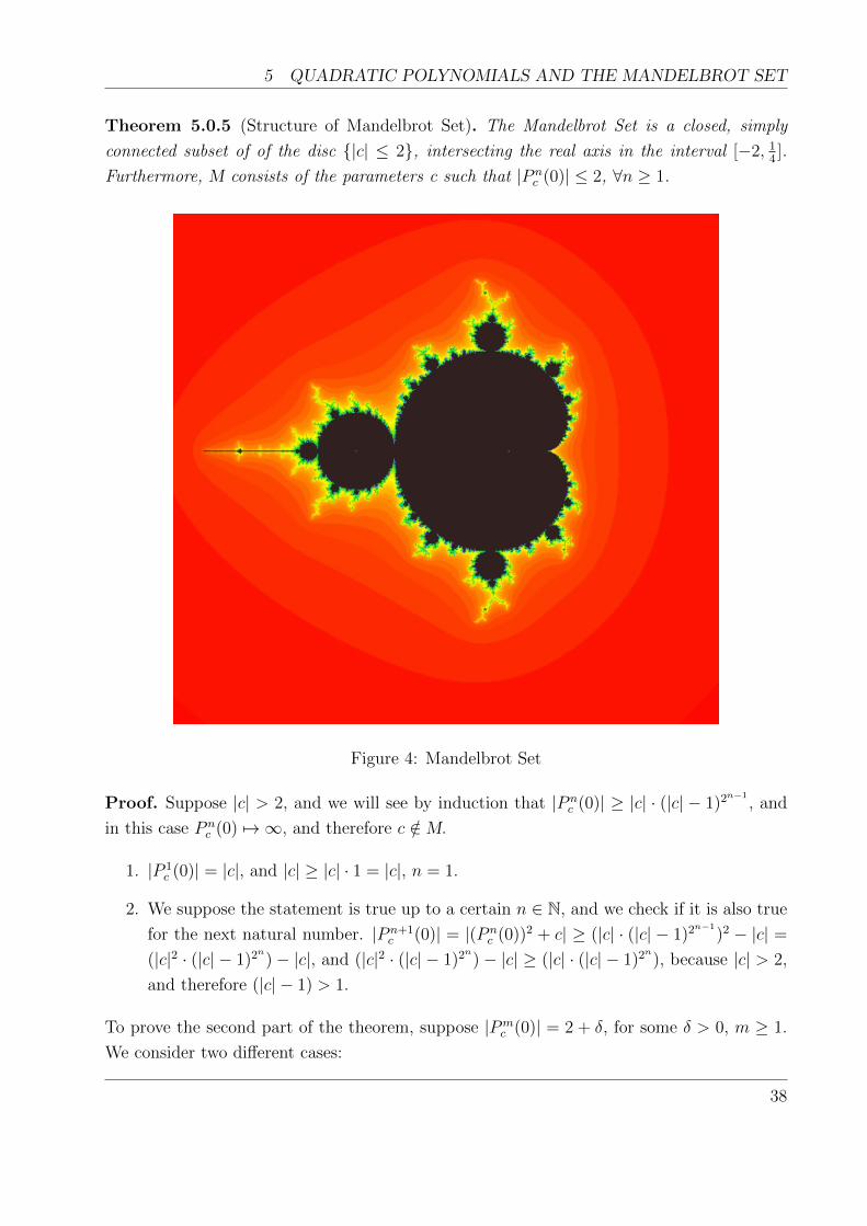
5 QUADRATIC POLYNOMIALS AND THE MANDELBROT SET
Theorem 5.0.5 (Structure of Mandelbrot Set). The Mandelbrot Set is a closed, simply
connected subset of of the disc |c| ≤ 2, intersecting the real axis in the interval [−2, 14].
Furthermore, M consists of the parameters c such that |P nc (0)| ≤ 2, ∀n ≥ 1.
Figure 4: Mandelbrot Set
Proof. Suppose |c| > 2, and we will see by induction that |P nc (0)| ≥ |c| · (|c| − 1)2
n−1, and
in this case P nc (0) 7→ ∞, and therefore c /∈ M.
1. |P 1c (0)| = |c|, and |c| ≥ |c| · 1 = |c|, n = 1.
2. We suppose the statement is true up to a certain n ∈ N, and we check if it is also true
for the next natural number. |P n+1c (0)| = |(P n
c (0))2 + c| ≥ (|c| · (|c| − 1)2n−1
)2 − |c| =(|c|2 · (|c| − 1)2
n)− |c|, and (|c|2 · (|c| − 1)2
n)− |c| ≥ (|c| · (|c| − 1)2
n), because |c| > 2,
and therefore (|c| − 1) > 1.
To prove the second part of the theorem, suppose |Pmc (0)| = 2 + δ, for some δ > 0, m ≥ 1.
We consider two different cases:
38

5 QUADRATIC POLYNOMIALS AND THE MANDELBROT SET
1. if |c| = |Pc(0)| > 2, then c /∈ M
2. if |c| ≤ 2, then |Pm+1c (0)| ≥ (2+δ)2−2 ≥ 2+4 ·δ, and by induction we get |Pm+k
c (0)| ≥2 + 4k · δ 7→ ∞, and again c /∈ M
From these second part of the theorem, it follows that M is closed.
As for the final statement, if c is real, Pc(0)− x has no real roots if c > 14, one root at x = 1
2
if c = 14
and two real roots for each c < 14. Therefore, if c > 1
4, P n
c (0) is increasing, and tends
to infinity, since any finite limit should satisfy P nc (0) = x, for some n ≥ 1, so c /∈ M. Now, if
f c ≤ 14, we consider a = 1+
√1−4·c2
the larger root of Pc(0)− x, and if c also satisfies c ≥ −2,
then a ≥ |c| = Pc(0). Then, P nc (0) ≤ a implies |P n+1
c (0)| = |P nc (0)2 + c| ≤ a2 + c = a, and
the sequence is bounded. All in all, M ∩ R = [−2, 14].
Theorem 5.0.6. For each λ, |λ| < 1, there is a unique c = c(λ) such that Pc has a fixed
point with multiplier λ. The values, c, for which Pc has an attracting fixed point form a
cardioid C ⊂M, and ∂C ⊂ ∂M. If c ∈ C, then Jc is a quasicircle(∗).
Proof. The fixed points of Pc are zc = 1±√1−4c2
, with multiplier λ(c) = 2·zc. Since c = λ2− λ2
4,
the condition |λ(c)| < 1 corresponds in the c-plane to the cardioid:
C = λ2− λ2
4: λ < 1
It is a subset of M called the main cardioid of M. Since the function λ2− λ2
4is one-to-one in
the closed unit disk, we get the uniqueness.
Let W be the component of the interior of M containing C. By theorem 5.0.5 the polynomials
fn(c) = P nc (0) are uniformly bounded in W, and they converge to the attracting fixed point
zc on C. However, if c /∈ C, then zc is a repelling fixed point, and we can not have P nc (0) 7→ zc
unless P nc (0) = zc for some n large enough. As this can occur only in a countable set, we
conclude that W = C
Theorem 5.0.7. Suppose there is an attracting cycle of length m for Pa. Then a belongs to
the interior of M. If W is the component of the interior of M containing a, then Pc has an
attracting cycle z1(c), ..., zn(c) of length m for all c ∈W, where each zj(c), j ∈ 1, ...,mdepends analytically on c.
Proof. Let z1(a) be an attracting periodic point of period m for a. Applying the implicit
function theorem to Q(z, c) = Pmc (z) − z, we obtain an attracting periodic point z1(c) for
Pc of period m, which depends analytically on c in a neighborhood of a. In particular,
a belongs to the interior of M, and we name W the component of M containing a. The
39

5 QUADRATIC POLYNOMIALS AND THE MANDELBROT SET
sequence fj(c) = P jmc (0) is bounded, and therefore normal, in W, and it converges at a to
some point in the cycle z1(a), say to z1(a) itself.
Since z1(c) is attracting, fj(c) converges to z1(c) for c near a. By normality, fj(c) converges
on W to some analytical function, g(c) which satisfies
Q(g(c), c) = 0 near a(and therefore in W)
We know that g(c) can be a repelling periodic point for a fixed c ∈W only if P jmc (0) actually
coincides with g(c) for j sufficiently large. This occurs a set which is at most countable. Since
the multiplier, λ(c), of the cycle is analytic, we conclude that |λ| < 1 on W, that is, the
cycle of g(c) is attracting for all c ∈W.
The components of the interior of M associated with attracting cycles are called hyperbolic
components of the interior of M. This name comes from the fact that Pc is hyperbolic when
c /∈ M or Pc has an attracting cycle. It is not known whether the hyperbolic components
completely fill out the interior of M, but it do is known that they are dense in the interior
of M.
Definition 5.0.8. A point c ∈M is called a Misiurewicz25 point if 0 is strictly preperiodic,
that is, P nc (0) = P k
c (0) for some n > k > 0, but P nc (0) 6= 0 for all n ≥ 1
A polynomial Qc can have, at most, one attracting cycle in C. It follows that Qc is hyperbolic
iff Qc has an attracting cycle in C, or if the orbit of the critical point is attracted to the
superattracting fixed point at ∞. In this case, the c-value is called a hyperbolic parameter.
If Qc0 has an attracting p-cycle in C, it follows from the Implicit Function Theorem that this
p-cycle moves holomorphically for parameter values close to c0 and the cycle is still attracting.
As a consequence, c0 ∈ int(M). The maximal open set containing c0, Ω, of parameter for
which a p-cycle exists and remains attracting, is called a hyperbolic component of M.
It is not known yet if all the components of int(M) are hyperbolic. However, there is a
conjecture, which has been proved true for parameters in the real line:
Conjecture 5.0.9 (Hyperbolic Conjecture). The interior of M is equal to the union of all
the hyperbolic components:
int(M) =⋃
Ω
for every Ω which is a hyperbolic component.
25Michael Misiurewicz(1948 - ) is a Polish mathematician who is known for his contributions to dynamical
systems and fractal geometry.
40

5 QUADRATIC POLYNOMIALS AND THE MANDELBROT SET
Definition 5.0.10 (Multiplier map). Given a hyperbolic component, Ω, of period p, the
multiplier map is defined as
Λ : Ω 7→ D
satysfing Λ(c) = (Qpc)′(z(c)), where z(c), for each c ∈ Ω, denotes a point in the attracting
p-cycle so that c 7→ z(c) is holomorphic. It follows then that Λ is holomorphic.
Theorem 5.0.11 (Multiplier map). Let Ω be a hyperbolic component of M of period p. Then,
the multiplier map is a conformal isomorphism which extends continuously to Λ : Ω 7→ D.
It follows from this theorem that all hyperbolic components are topological discs, each with a
center, that is, the unique parameter value for which the attracting cycle is superattracting,
i.e. Λ−1(0).
Definition 5.0.12. The boundary of Ω has a unique point, called the root of Ω, for which
the multiplier of the p-cycle is exactly 1.
Attached to every boundary parameter for which the multiplier of the cycle has derivative
e2·π·i·rs we find a new hyperbolic component of period p · s. This explains part of the fractal
structure which we encounter near any point of the boundary of M.
Theorem 5.0.13 (Parameters in ∂M). For the boundary of the Mandelbrot Set, we have
the following results:
1. Misiurewicz points are dense in ∂M.
2. For each c ∈ ∂M there exists a sequence cnn of centers of hyperbolic components
such that cn 7→ c as n 7→ ∞.
3. If Qc has a parabolic, Siegel or Cremer cycle, then c ∈ ∂M.
Of special interest are the parameter values of c for which Pc has a superattracting cycle.
The critical point 0 must be in this set, so these are precisely the c's for which 0 is periodic,
that is, the solutions of P nc (0) = 0.
Theorem 5.0.14. The values of c ∈ M corresponding to superattracting cycles cluster on
the entire boundary ∂M. In particular, the interior of M is dense in M.
Proof. Let U be a disk that meets ∂M and such that 0 /∈ U. Suppose U contains no value c
for which 0 is periodic and consider the branch of√−c defined on U. We have P n
c (0) 6=√−c,
or else P nc (0) = 0 and 0 is periodic. Therefore, fn(c) = Pnc (0)√
−c omits the values 0, 1 and ∞on U, hence is a normal sequence on U. But, since U meets ∂M, it contains both values c
with fn(c) bounded and with fn(c) 7→ ∞, so the sequence can not be normal.
41
5 QUADRATIC POLYNOMIALS AND THE MANDELBROT SET
The most important conjecture about the Mandelbrot Set is about a topological property:
Conjecture 5.0.15 (MLC). The Mandelbrot Set, M, is locally connected.
This conjecture would imply the HC conjecture as well, and is the focus of many studies
currently.
42
6 SINGULAR PERTURBATIONS OF CUBIC MILNOR POLYNOMIALS
6 SINGULAR PERTURBATIONS OF CUBIC
MILNOR POLYNOMIALS
In the previous section, we have studied the parameter space of the map
f(z) = z2 + c, c ∈ C
And now we want to take a look at the changes that this, and other families of polynomial
maps, experience when we add a pole singularity.
6.1 SINGULAR PERTURBATIONS
Robert Devaney, Daniel Look and David Uminsky studied the behavior of the Julia Set of
functions in the family of rational maps given by
Fλ(z) = zn + λzd
where n, d ∈ Z and n ≥ 2, d ≥ 1. For λ = 0, we get the map z 7→ zn, which has a known
and well understood behavior, and for which the Julia set is also clear.
However, when λ 6= 0, we produce several modifications to the initial map:
1. The map Fλ now has degree n+ d.
2. The origin is no longer a fixed point, but a pole instead.
3. There are n+ d new critical points, in addition to the original critical points at 0 and
∞. The orbits of the critical points at∞ and the origin are fixed, and eventually fixed
respectively, so their behavior is completely determined. As for the orbits of all the
other critical points, they behave symmetrically with respect to rotation through angle2·πn+d
, so essentially we have only one additional ”free” critical orbit for each of these
maps.
For the family Fλ, the point at ∞ is still a superattracting fixed point, and therefore it
still has an immediate basin of attraction, which we denote by B. However, this basin of
attraction may consist of infinitely many disjoint preimages of the immediate basin of∞. In
particular, the component of the basin that contains 0 may be disjoint from B, and in this
case we denote this component by T. The following result was established:
Theorem 6.1.1 (The escape Trichotomy). Suppose the orbits of the free critical points of
Fλ tend to ∞. Then
43

6 SINGULAR PERTURBATIONS OF CUBIC MILNOR POLYNOMIALS
1. If one of the critical values lies in B, then J(Fλ) is a Cantor Set and Fλ|J(Fλ) is a
one-sided shift on n+ d symbols. Otherwise, J(Fλ) is connected and the preimage T is
disjoint from B.
2. If one of the critical points lies in T, then J(Fλ) is a Cantor set of simple closed
curves(quasicircles).
3. If one of the critical values lies in a preimage of T, then J(Fλ) is a Sierpinski curve(∗).
Figure 5: The Julia Set for z4 + 0.3z4
, which is a Cantor Set.
The proofs to all the results found by Devaney, Look and Uminsky can be found in [8].
6.2 MILNOR POLYNOMIALS
Any cubic polynomial is of the form P (z) = A·z3+B ·z2+C ·z+D, for some A,B,C,D ∈ R.
However, we can conjugate P (z) to S(z) = z3 + α · z2 + β · z + γ by a linear map, making
it monic. Furthermore, by an affine conjugacy, we can make S(z) centered (the sum of its
critical points is 0), therefore obtaining the condition α = 0, so that we get the polynomial
R(z) = z3+β ·z+γ. Its critical points are x± = ±√−12β6
, and if we write β = −3 ·a2 for some
a ∈ R, the critical points become x± = ±a. All in all, we have obtainedQ(z) = z3−3·a2·z+γ,
conjugated to the original polynomial P (z). Their natural parameter space is C2, and one
way to try to understand it is by taking dynamically meaningful one-dimensional slices. In
44

6 SINGULAR PERTURBATIONS OF CUBIC MILNOR POLYNOMIALS
Figure 6: The Julia Set for z4 + 0.04z4
, which is a Cantor Set of circles.
Figure 7: The parameter space for z4 + λz4
.
[14], Milnor considers the slice formed by those polynomials for which a is a fixed point, which
makes b = 2·a3+a, therefore resulting in polynomials of the from Pa(z) = z3−3·a2·z+2·a3+a.
If we move the superattracting fixed point to 0 with the transformation z 7→ z − a, and use
the conjugation z 7→ −13a· z, we get Pa(z) = 9a2 · z2 · (z − 1). Finally, we can write b = 9a2,
so that the resulting polynomial has the form Pb(z) = b · z2 · (z− 1). The new critical points
are now located at z = 0 and z = 23. We can observe that P ′b(0) = 0, and therefore 0 is
45
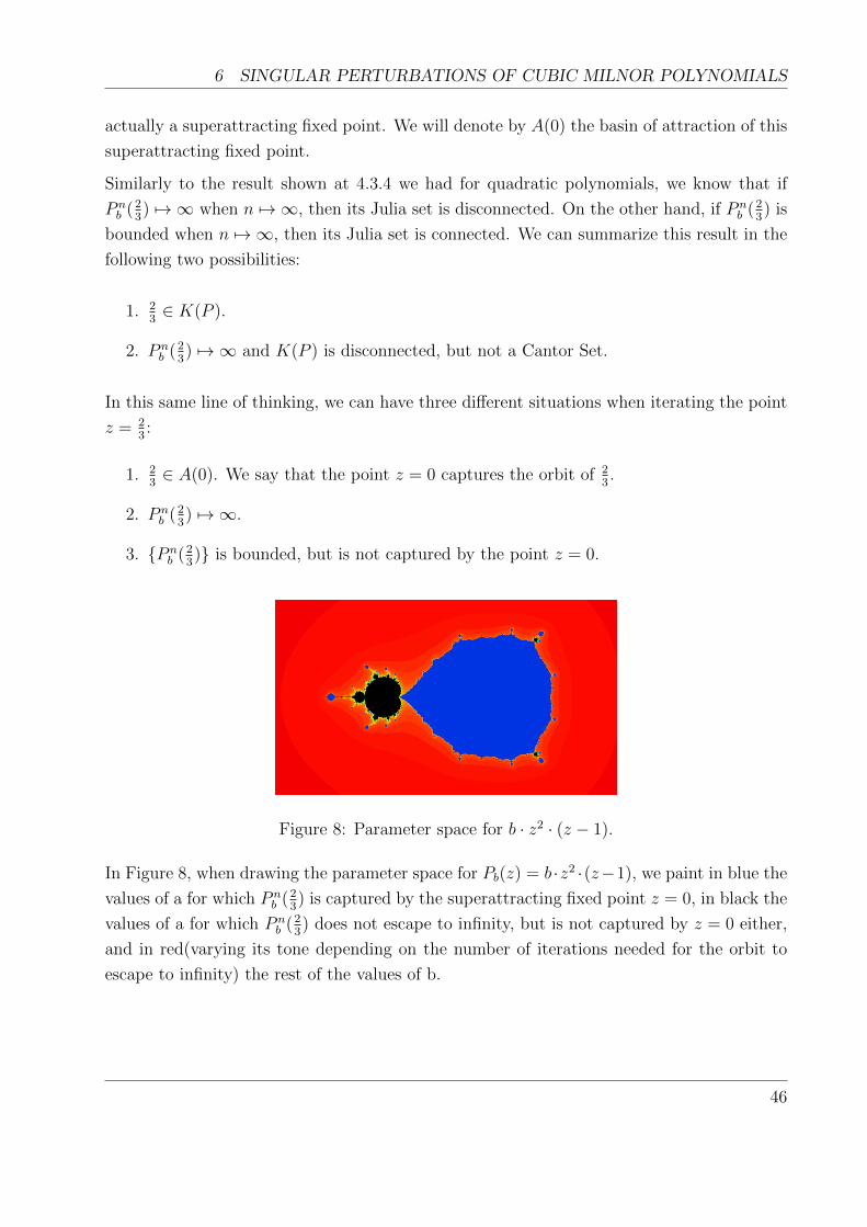
6 SINGULAR PERTURBATIONS OF CUBIC MILNOR POLYNOMIALS
actually a superattracting fixed point. We will denote by A(0) the basin of attraction of this
superattracting fixed point.
Similarly to the result shown at 4.3.4 we had for quadratic polynomials, we know that if
P nb (2
3) 7→ ∞ when n 7→ ∞, then its Julia set is disconnected. On the other hand, if P n
b (23) is
bounded when n 7→ ∞, then its Julia set is connected. We can summarize this result in the
following two possibilities:
1. 23∈ K(P ).
2. P nb (2
3) 7→ ∞ and K(P ) is disconnected, but not a Cantor Set.
In this same line of thinking, we can have three different situations when iterating the point
z = 23:
1. 23∈ A(0). We say that the point z = 0 captures the orbit of 2
3.
2. P nb (2
3) 7→ ∞.
3. P nb (2
3) is bounded, but is not captured by the point z = 0.
Figure 8: Parameter space for b · z2 · (z − 1).
In Figure 8, when drawing the parameter space for Pb(z) = b ·z2 ·(z−1), we paint in blue the
values of a for which P nb (2
3) is captured by the superattracting fixed point z = 0, in black the
values of a for which P nb (2
3) does not escape to infinity, but is not captured by z = 0 either,
and in red(varying its tone depending on the number of iterations needed for the orbit to
escape to infinity) the rest of the values of b.
46

6 SINGULAR PERTURBATIONS OF CUBIC MILNOR POLYNOMIALS
6.3 SINGULAR PERTURBATIONS OF MILNOR CUBIC POLY-
NOMIALS
We add a pole singularity at z = 0 to the map Pb(z), controlling the size of the perturbation
with the parameter λ, obtaining a family of functions of the form
Pb,λ(z) = b · z2 · (z − 1) + λz3
Our aim is to a do a numerical exploration, looking for interesting topological objects in form
of Julia Sets. After adding a pole singularity, we now have a rational function of degree 6,
with 9 critical points, one of which is the point at infinity with multiplicity 3. By computing
P ′b,λ(z), we see that its critical points satisfy
b · z6 − 23· b · z5 = λ
When λ = 0, this equation has 6 solutions: the origin with multiplicity 5, and z = 23
with
multiplicity 1. By continuity, for small enough values of |λ| the 6 solutions of the equation
become simple zeros of P ′b,λ(z) which are approximately symmetrically distributed around
the origin and 23. Therefore, although we can not compute the exact value of the new critical
points, we will iterate z = 23, because for |λ| small enough, the qualitative behavior of the
orbit P nb,λ(z) is the same.
The point at∞ is a superattracting fixed point for Pb,λ(z), and, in a neighborhood of infinity,
Pb,λ(z) is conjugate to z 7→ z3, so we have an immediate basin of attraction, B, at ∞. Since
Pb,λ(z) has a pole of order 3 at 0, there is an open neighborhood of 0 that is mapped 3 to
1 onto a neighborhood of ∞ in B. If B does not contain this neighborhood, then there is a
disjoint open set T about 0 that is mapped 3 to 1 onto B. We call T the trap door since any
point whose orbit eventually enters B must pass through T en-route to B. Since the degree
of Pb,λ(z) is 6, all points in the preimage of B lie either in B or in T.
In Figure 9 we see that, when we add a pole singularity at the superattracting fixed point
z = 0 to Pb(z), for |λ| small, all the components previously painted in blue suffer a dramatic
change. On the other hand, both the components painted in black or red, suffer little to
no qualitative variation. This happens because this perturbation is only truly meaningful in
a neighborhood of 0, and therefore all the values of b for which P nb,λ(
23) does not visit such
neighborhood of 0, have the same behavior as before. We can see three examples of very
different parameter spaces, one of which is formed by Sierpisnki curves, and the other two
which are Cantor Sets of circles, and the trap doors can also be observed, in form of red
47

6 SINGULAR PERTURBATIONS OF CUBIC MILNOR POLYNOMIALS
Figure 9: Comparison between the parameter space for b · z2 · (z − 1) + 10−5
z3(top left),
b · z2 · (z − 1) + 10−7
z3(top right) and b · z2 · (z − 1) + 10−11
z3(bottom center).
disks around z = 0. This image also shows that the iteration of z = 23
is a good enough
approximation, because the Mandelbrot-like shapes appear well shaped and detailed.
In figure 10, similarly to the Escape Trichotomy established by Devaney, Look and Uminsky,
we have included examples for each of the three type of Julia Sets described in that result:
a Cantor Set, a Cantor Set of circles and a Sierpinski curve.
One of the main reasons for choosing Milnor Cubic Polynomials as the object of study when
adding the pole singularity, was the fact that these functions already presented interesing
Julia Sets before the addition of the perturbation, and we wanted to see if such behavior
persisted afterward. In this direction, in figure 11 we see two examples of curious Julia Sets:
a disconnected Julia set which is not a Cantor Set and a structure very similar to a Sierpin-
ski carpet, but which can not be such object, because the boundaries of the complementary
domains are not Jordan Curves. We also see that not all critical points need to act in a
symmetrical way: here 4 of the critical points close to z = 0 form a periodic orbit of period
4, while the other converges to a fixed point.
48
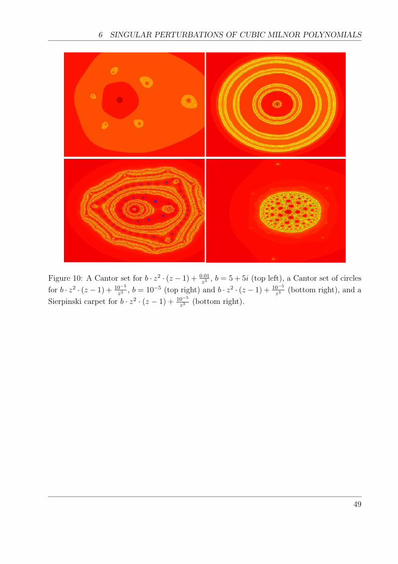
6 SINGULAR PERTURBATIONS OF CUBIC MILNOR POLYNOMIALS
Figure 10: A Cantor set for b · z2 · (z − 1) + 0.01z3
, b = 5 + 5i (top left), a Cantor set of circles
for b · z2 · (z − 1) + 10−5
z3, b = 10−5 (top right) and b · z2 · (z − 1) + 10−5
z3(bottom right), and a
Sierpinski carpet for b · z2 · (z − 1) + 10−5
z3(bottom right).
49

6 SINGULAR PERTURBATIONS OF CUBIC MILNOR POLYNOMIALS
Figure 11: The Julia Set for b · z2 · (z − 1) + 5.32264·10−06
z3, b = 5.55 (top left), and a zoomed
image of it (top right), and the Julia Set for b · z2 · (z − 1) + 10−5
z3, b = −8 (bottom center).
50

7 GLOSSARY
7 GLOSSARY
Conformal map A map f : U 7→ V is said to be conformal at a point u0 ∈ U if it pre-
serves oriented angles between curves through u0 with respected to their orientation.
In complex analysis, f is conformal ⇔ it is holomorphic and f ′(z) 6= 0 ∀z ∈ U .
Doubly connected A topological space, X, is said to be doubly connected if it is non-
empty, path-connected, and its first two homotopy groups vanish identically, that is,
if
πi(X) ' 0, i = 1, 2.
where the left-hand side denotes the i-th homotopy group.
Equicontinuous Let X and Y be metric spaces and let F be a set of maps
f : X 7−→ Y
We say that F is equicontinuous at a point a ∈ X if ∀ε > 0, there is some δ > 0 such
that if d(x, a) < δ, then d(f(x), f(a)) < ε, x ∈ X, ∀f ∈ F.
Generic point Given a topological space X, we say that a point p ∈ X is generic if the
closure of the singleton set p is X.
Lie group A Lie group is a group which is also a a differential manifold, with the property
that the group operations are compatible with the smooth structure.
Locally connected Let X be a topological space, and let x ∈ X. We say that X is locally
connected at x if, for every open set V containing x, there exists a connected, open set
U, x ∈ U ⊂ V .
Meromorphic function We say that a function f : U 7→ C is meromorphic, if it is holo-
morphic in all of U except for a set of isolated points(the poles of the function) at each
of which the function must have a Laurent series.
51
7 GLOSSARY
Mobius transformation Let a ∈ C, |a| ≤ 1. Then,
φa(z) = z−a1−a·z
is a Mobius transformation. φa is a conformal self-map of the unit disk for each a,
and any conformal self-map of the unit disk to itself is a composition of a Mobius
transformation with a rotation.
Path A path in a topological space X, is a continuous function from a closed interval to X,
i.e, a continuous function f : I = [a, b] 7→ X, for some a, b ∈ R.
Pole Suppose U ⊂ C is an open set, p ∈ U and f : U \ p 7→ C is an holomorphic function.
If there exists a holomorphic function g : U 7→ C such that g(p) 6= 0 and a positive
integer, n ≥ 0, n ∈ N such that for all z ∈ U \ p, f can be expressed as
f(z) = g(z)(z−p)n
we say that p is a pole of f.
Quasicircle A quasicircle is the image of a circle by a quasiconformal mapping of the ex-
tended complex plane.
Quasiconformal mapping Let f : C 7→ C, and we define the dilatation of the mapping f
at the point z as
Df (z) = |fz |+|fz ||fz |−|fz | ≥ 1
and we define the maximal dilatation of the mapping as
Kf = supzDf (z)
We say that f is quasiconformal if is absolutely continuous on lines, and its maximal
dilatation is finite.
Sierpinski curve A Sierpinski curve is a planar set that is homeomorphic to the Sierpinski
carpet fractal.
52
7 GLOSSARY
Simply connected We say that a set is simply connected if it is path-connected, and it’s
fundamental group is the trivial group.
Uniform convergence A sequence of functions fn, n = 1, 2, 3, ... is said to be uniformly
convergent to f for a set, E, of values of x if, ∀ε > 0, there exists n0 ∈ N such that
|fn(x)− f(x)| < ε, ∀n ≥ n0, ∀x ∈ E
Winding number The winding number of a closed curve around a point is an integer show-
ing the number of counterclockwise travels of the curve around the point. Formally,
given a closed curve γ, and a point z0 /∈ γ, if such curve does not pass through the
origin (if it does, we can redefine the coordinate system), we can express γ in polar
coordinates, making it dependent of r(t), θ(t), 0 ≤ t ≤ 1, so that, as the curve is closed,
θ(1)− θ(0) = 2π · k, for some k ∈ Z. Finally we define the winding number as
winding number := θ(1)−θ(0)2π
53
REFERENCES
References
[1] Abate, Marco. Fatou flowers and parabolic components [online]. Dipartimento di Matem-
atica, Universita di Pisa, 2015 [last consulted: March 23, 2016]. It requires Ac-
robat Reader. Available at : http://www.dm.unipi.it/ abate/articoli/artric/files/A-
bateParabolicCurvesSurveyb.pdf.
[2] Antolin, Omar. Iteration of rational functions
[3] Beardon, Alan. Iteration of rational functions. Springer-Verlag.
[4] Branner, Bodil and Fagella, Nuria. Quasiconformal surgery in holomorphic dynamics.
Cambridge university press, 2014 .
[5] Carlesson, Lennart and Gamelin, Theodore. Complex dynamics. Springer-Verlag.
[6] Conway, John. Functions of one complex variable I. Springer-Verlag, 1978.
[7] Conway, John. Functions of one complex variable II. Springer-Verlag, 1995.
[8] Devaney, Robert; Look, Daniel; Uminsky, David. The escape trichotomy for singularly
perturbed rational maps. Indiana University Mathematics Journal, 2005.
[9] Garijo, Antonio; Godillon, Sebastien; On McMullen-like mappings. 2014.
[10] Garijo, Antonio; Marotta, Sebastian; Rusell, Elizaabeth. Singular perturbations in the
quadratic family with multiple poles. Journal od Difference Equations and Applications
Vol. 19, 2013.
[11] Jarque, Xavier and Fagella, Nuria. Iteracion compleja y fractales. Vicens Vives, 2007.
[12] Marsden, Jerrold and Hoffman, Michael. Basic complex analysis. W.H. Freeman, New
York, 1999.
[13] Milnor, John. Dynamics in one complex variable : Introductory lectures. Princeton Uni-
versity Press, 2006.
[14] Milnor, John. Remarks on iterated cubic maps. Experimental mathematics Vol I, 1992.
54