Item response Theory.pdf
31
0 NOTES ITEM RESPONSE THEORY (AN INTRODUCTION) Contents 1. What is item analysis in general? .......................................................................................................... 1 2. Classical Test Theory ............................................................................................................................ 3 2.1 Classical Test Theory Statistics .................................................................................................... 4 2.2 Classical Test Theory vs Latent Trait Models .............................................................................. 4 2.3 Latent Trait Models....................................................................................................................... 6 3. Item Response Theory .......................................................................................................................... 7 3.1 Three Basics Components of IRT ................................................................................................. 7 3.1 Item Response Functions (IRF) .................................................................................................... 8 3.2 Item Parameters Location (b) ........................................................................................................ 8 3.3 Item Parameters Discrimination (a) .............................................................................................. 9 3.4 Item Parameters Guessing (c) ..................................................................................................... 10 3.5 Item Parameters Upper asymptote (d)......................................................................................... 11 3.6 Item Response Function Model .................................................................................................. 12 3.7 IRT - Test Response Curve ......................................................................................................... 23 3.8 Item Information Functions (IIF) ................................................................................................ 24 3.9 Item Response Theory Example ................................................................................................. 25 3.10 Invariance.................................................................................................................................... 25 3.11 IRT Assumptions ........................................................................................................................ 26 3.12 IRT Applications ......................................................................................................................... 27 4. Rasch Models vs Item Response Theory Models ............................................................................... 30 5. References ........................................................................................................................................... 30
-
Upload
syahida-iryani -
Category
Documents
-
view
97 -
download
1
description
Education
Transcript of Item response Theory.pdf

0
NOTES
ITEM RESPONSE THEORY
(AN INTRODUCTION)
Contents 1. What is item analysis in general? .......................................................................................................... 1
2. Classical Test Theory ............................................................................................................................ 3
2.1 Classical Test Theory Statistics .................................................................................................... 4
2.2 Classical Test Theory vs Latent Trait Models .............................................................................. 4
2.3 Latent Trait Models ....................................................................................................................... 6
3. Item Response Theory .......................................................................................................................... 7
3.1 Three Basics Components of IRT ................................................................................................. 7
3.1 Item Response Functions (IRF) .................................................................................................... 8
3.2 Item Parameters Location (b) ........................................................................................................ 8
3.3 Item Parameters Discrimination (a) .............................................................................................. 9
3.4 Item Parameters Guessing (c) ..................................................................................................... 10
3.5 Item Parameters Upper asymptote (d)......................................................................................... 11
3.6 Item Response Function Model .................................................................................................. 12
3.7 IRT - Test Response Curve ......................................................................................................... 23
3.8 Item Information Functions (IIF) ................................................................................................ 24
3.9 Item Response Theory Example ................................................................................................. 25
3.10 Invariance .................................................................................................................................... 25
3.11 IRT Assumptions ........................................................................................................................ 26
3.12 IRT Applications ......................................................................................................................... 27
4. Rasch Models vs Item Response Theory Models ............................................................................... 30
5. References ........................................................................................................................................... 30

1
1. What is item analysis in general?
Item analysis provides a way of measuring the quality of questions - seeing how
appropriate they were for the respondents and how well they measured their ability/trait.
It also provides a way of re-using items over and over again in different tests with prior
knowledge of how they are going to perform; creating a population of questions with
known properties (e.g. test bank)
Whatever the type of test, standardized, ability or personality, a post hoc (after-the-fact)
analysis of the results should be carried out.
The major purpose of item analysis is to improve tests by revising or eliminating
ineffective items, and to increase our understanding of a test (why a test is reliable, valid,
or not). Another important aspect of item analysis relates specifically to achievement
tests. Here, item analysis can provide important diagnostic information on what
examinees have learned and what they have not learned.
Item analysis refers to a varied group of statistics that are computed for each item on a
test. These item statistics help to determine the role each item plays with respect to the
entire test.
There are many different types/procedures for determining item statistics. The procedure
employed in evaluating an item's effectiveness depends to some extent on the researcher's
preference and on the purpose of the test.
Let’s consider some of these item analysis procedures. It is a good deal of discussion on
achievement/multiple choice types of tests to illustrate the item-analysis methods. Please
remember that these concepts can also apply to other types of test (e.g., personality).

2
Figure 1: Item Analysis Map

3
2. Classical Test Theory
Classical Test Theory (CTT) - analyses are the easiest and most widely used form of
analyses. The statistics can be computed by readily available statistical packages (or
even by hand)
Classical Analyses are performed on the test as a whole rather than on the item and
although item statistics can be generated, they apply only to that group of students on that
collection of items
Classical test theory is a bit of a misnomer; there are actually several types of CTTs. The
foundation for them all rests on aspects of a total test score made up of multiple items.
Most classical approaches assume that the raw score (X) obtained by any one individual
is made up of a true component (T) and a random error (E) component:
X = T + E.
CTT is based on the true score model. The true score of a person can be found by taking
the mean score that the person would get on the same test if they had an infinite number
of testing sessions.
The assumptions in the CTT are that the error:
a) Is normally distributed
b) Uncorrelated with true score
c) Has a mean of Zero
In this formulation, where error scores are defined, true score is the difference between
test score and error score.
True score is easily shown to be the expected test score across parallel forms. In other
formulations of this model, true score is defined as the expected test score over parallel
4
forms, and then the resulting properties of error are derived. In either case, the resulting
model is the same and has found wide-spread use in testing practice.
Some researchers prefer the latter formulation because it results in defining the concept
of central interest, true score, rather than having it obtained as the difference between test
score and error score.
2.1 Classical Test Theory Statistics
Difficulty (item level statistic)
Discrimination (item level statistic)
Reliability (test level statistic)
2.2 Classical Test Theory vs Latent Trait Models
Classical analysis has the test (not the item) as its basis. Although the statistics generated
are often generalised to similar students taking a similar test; they only really apply to
those students taking that test
Latent trait models aim to look beyond that at the underlying traits which are producing
the test performance. They are measured at item level and provide sample-free
measurement.
Differences Between Theories and Models
a) Classical test models are often referred to as "weak models" because the
assumptions of these models are fairly easily met by test data. (Though it must be
mentioned that not all models within a classical test theoretic framework are
"weak."
Permit examinees to be compared even when
the examinees have not taken the same items.

5
b) Item response models are referred to as strong models, because the underlying
assumptions are stringent and therefore less likely to be met with test data. For
example, the popular one-, two-, and three-parameter logistic models make the
strong assumption that the set of items that compose the test are measuring a single
common trait or ability.
c) Classical test models do not make such a strong assumption. It is only necessary to
assume that the factor structure, whatever it is, is common across parallel forms.
d) What follows are presentations of classical test theory and item response theory and
their related models and concepts, and a comparison of the two statistical
frameworks.
Importance of Test Theories and Models
a) A good theory or model can help in understanding the role that measurement errors
play in
estimating examinee ability and how the contributions of error might be
minimized (e.g., lengthening a test),
correlations between variables (see for example the disattenuation formulas),
and
reporting true scores or ability scores and associated confidence bands.
b) Different theories and models will handle errors differently. For example, errors
might be assumed to be normally distributed in one model, whereas no distributional
assumptions about errors are made in another. In one model, the size of
measurement errors might be assumed to be constant across the test-score scale (i.e.,
the standard error of measurement). In another, the size of errors might be assumed
to be related to the examinee's true score i.e., the binomial error model). The

6
specifications about error in a model will have substantial impact on how error
scores are estimated and reported.
c) A good test theory or model can also provide a frame of reference for doing test
design work or solving other practical problems. A good test model might specify
the precise relationships among test items and ability scores so that careful test
design work can be done to produce desired test score distributions and errors of the
size that can be tolerated. For example, in computer adaptive testing, a test model
that closely links ability estimates to item statistics is needed to guide the item
selection process. Items should be selected at any point in the testing process that
provides maximum information about examinee ability.
d) In this application, a model is needed that places persons and items on a common
scale (this is done with item response theory models). In this way, at each stage in
the computer adaptive testing process, items can be selected that provide the most
useful information about examinee ability.
2.3 Latent Trait Models
Latent trait models have been around since the 1940s, but were not widely used
until the 1960s. Although theoretically possible, it is practically unfeasible to use
these without specialized software.
They aim to measure the underlying ability (or trait) which is producing the test
performance rather than measuring performance of a person.
This leads to them being sample-free. As the statistics are not dependant on the
test situation which generated them, they can be used more flexibly.

7
3. Item Response Theory
Item Response Theory (IRT) – refers to a family of latent trait models used to establish
psychometric properties of items and scales
Sometimes referred to as modern psychometrics because in large-scale education
assessment, testing programs and professional testing firms IRT has almost completely
replaced CTT as method of choice
IRT has many advantages over CTT that have brought IRT into more frequent use.
Item response theory is a general statistical theory about examinee item and test
performance and how performance relates to the abilities that are measured by the items
in the test.
Item responses can be discrete or continuous and can be dichotomously or
polychotomously scored; item score categories can be ordered or unordered; there can be
one ability or many abilities underlying test performance; and there are many ways (i.e.,
models) in which the relationship between item responses and the underlying ability or
abilities can be specified.
In this module, only a few of the models that (a) assume a single ability underlies test
performance, (b) can be applied to dichotomously scored data, and (c) assume the
relationship between item performance and ability is given by a one-, two-, or three-
parameter logistic function will be considered.
3.1 Three Basics Components of IRT
a) Item Response Function (IRF) – Mathematical function that relates the latent trait
to the probability of endorsing an item
b) Item Information Function – an indication of item quality; an item’s ability to
differentiate among respondents

8
c) Invariance – position on the latent trait can be estimated by any items with know
IRFs and item characteristics are population independent within a linear
transformation
3.1 Item Response Functions (IRF)
Item Response Function (IRF) - characterizes the relation between a latent variable
(i.e., individual differences on a construct) and the probability of endorsing an item.
The IRF models the relationship between examinee trait level, item properties and
the probability of endorsing the item.
Examinee trait level is signified by the greek letter theta () and typically has mean
= 0 and a standard deviation = 1.
IRFs can then be converted into Item Characteristic Curves (ICC) which are
graphical functions that represent the respondents ability as a function of the
probability of endorsing the item.
3.2 Item Parameters Location (b)
An item’s location is defined as the amount of the latent trait needed to have a .5
probability of endorsing the item.
The higher the “b” parameter the higher on the trait level a respondent needs to be
in order to endorse the item
Analogous to difficulty in CTT
Like Z scores, the values of b typically range from -3 to +3
9
3.3 Item Parameters Discrimination (a)
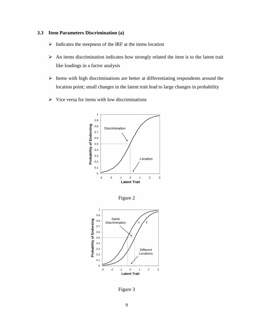
Indicates the steepness of the IRF at the items location
An items discrimination indicates how strongly related the item is to the latent trait
like loadings in a factor analysis
Items with high discriminations are better at differentiating respondents around the
location point; small changes in the latent trait lead to large changes in probability
Vice versa for items with low discriminations
Figure 2
Figure 3
0
0.1
0.2
0.3
0.4
0.5
0.6
0.7
0.8
0.9
1
-3 -2 -1 0 1 2 3
Latent Trait
Pro
bab
ilit
y o
f E
nd
ors
ing
.
Location
Discrimination
0
0.1
0.2
0.3
0.4
0.5
0.6
0.7
0.8
0.9
1
-3 -2 -1 0 1 2 3
Latent Trait
Pro
bab
ilit
y o
f E
nd
ors
ing
.
Same Discrimination
Different Locations
1 2

10
Figure 4
3.4 Item Parameters Guessing (c)
The inclusion of a “c” parameter suggests that respondents very low on the trait
may still choose the correct answer.
In other words respondents with low trait levels may still have a small probability
of endorsing an item
This is mostly used with multiple choice testing.
Figure 5
0
0.1
0.2
0.3
0.4
0.5
0.6
0.7
0.8
0.9
1
-3 -2 -1 0 1 2 3
Latent TraitP
rob
ab
ilit
y o
f E
nd
ors
ing
.
Different Discriminations
Different Locations
1
2
0
0.1
0.2
0.3
0.4
0.5
0.6
0.7
0.8
0.9
1
-3 -2 -1 0 1 2 3
Latent Trait
Pro
bab
ilit
y o
f E
nd
ors
ing
.
Different Locations
Different Discriminations
Lower Asymptote
1
2

11
3.5 Item Parameters Upper asymptote (d)
The inclusion of a “d” parameter which is inattention suggests that respondents
very high on the latent trait are not guaranteed (i.e. have less than 1 probability) to
endorse the item.
Often an item that is difficult to endorse (e.g. suicide as an indicator of
depression)
Figure 6
-3 -2 -1 0 1 2 30
0.1
0.2
0.3
0.4
0.5
0.6
0.7
0.8
0.9
1
Trait Level
Pro
babili
ty
2plm
3plm
4plm

12
3.6 Item Response Function Model
3.6.1 The 1-parameter logistic model
The equation for the Rasch model is given by the following:
Where e is constant 2.718
represents examinee trait level (ability level)
b is the item difficulty that determines the location of the IRF
L = a( - b) is the logistic deviate (logit), here, a = 1
If the item discrimination is set to 1.0 (or any constant) the result is a 1PL.
It should be noted that a discrimination parameter was used in equation, but because it
always has a value of 1.0, it usually is not shown in the formula.
A 1PL assumes that all scale items relate to the latent trait equally and items vary only in
difficulty (equivalent to having equal factor loadings across items).
Computational Example
Again the illustrative computations for the model will be done for the single ability level -
3.0. The value of the item difficulty parameter is:
b = 1.0.
The first term computed is the logit, L, where:
L = ( - b)
bb
b
ee
ebXP
1
1
1,1

13
Substituting the appropriate values yields:
L = 1.0 (-3.0 - 1.0) = -4.0
Next, the e to the x term is computed, giving:
EXP(-L) = 54.598
The denominator of the equation can be computed as:
1 + EXP(-L) = 1.0 + 54.598 = 55.598
Finally, the value of P() can be obtained and is:
P(0) = 1/(1 + EXP(-L)) = 1/55.598 = .02
Thus, at an ability level of -3.0, the probability of responding correctly to this item is .02. Table 1
shows the calculations for seven ability levels. You should perform the computations at several
other ability levels to become familiar with the model and the procedure. The item characteristic
curve corresponding to the item in Table 1 is shown below.

14
Table 1: Calculations for the one-parameter model, b = 1.0
Figure 7: Item characteristic curve for a one-parameter model with b = 1.0
15
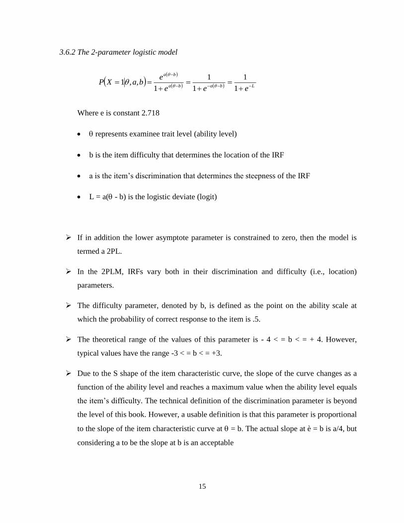
3.6.2 The 2-parameter logistic model
Where e is constant 2.718
represents examinee trait level (ability level)
b is the item difficulty that determines the location of the IRF
a is the item’s discrimination that determines the steepness of the IRF
L = a( - b) is the logistic deviate (logit)
If in addition the lower asymptote parameter is constrained to zero, then the model is
termed a 2PL.
In the 2PLM, IRFs vary both in their discrimination and difficulty (i.e., location)
parameters.
The difficulty parameter, denoted by b, is defined as the point on the ability scale at
which the probability of correct response to the item is .5.
The theoretical range of the values of this parameter is - 4 < = b < = + 4. However,
typical values have the range -3 < = b < = +3.
Due to the S shape of the item characteristic curve, the slope of the curve changes as a
function of the ability level and reaches a maximum value when the ability level equals
the item’s difficulty. The technical definition of the discrimination parameter is beyond
the level of this book. However, a usable definition is that this parameter is proportional
to the slope of the item characteristic curve at = b. The actual slope at è = b is a/4, but
considering a to be the slope at b is an acceptable
Lbaba
ba
eee
ebaXP
1
1
1
1
1,,1

16
approximation that makes interpretation of the parameter easier in practice. The
theoretical range of the values of this parameter is - 4< = a < = + 4, but the usual range
seen in practice is -2.80 to +2.80.
Computational Example
To illustrate how the two-parameter model is used to compute the points on an item
characteristic curve, consider the following example problem. The values of the item
parameters are:
b = 1.0 is the item difficulty.
a = .5 is the item discrimination.
The illustrative computation is performed at the ability level = -3.0.
The first term to be computed is the logistic deviate (logit), L, where:
L = a ( - b).
Substituting the appropriate values yields:
L = .5 (-3.0 - 1.0) = -2.0.
The next term computed is e (2.718) raised to the power -L. If you have a pocket calculator
that can compute ex you can verify this calculation. Substituting yields:
EXP (-L) = EXP (2.0) = 7.389, where EXP represents .
Now the denominator of equation 2-1 can be computed as:
1 + EXP (-L) = 1 + 7.389 = 8.389.
Finally, the value of P() is:
P() = 1/(1 + EXP (-L)) = 1/8.389 = .12.

17
Thus, at an ability level (T) of -3.0, the probability of responding correctly to this item is .12.
From the above, it can be seen that computing the probability of correct response at a given
ability level is very easy using the logistic model. Table 2-1 shows the calculations for this
item at seven ability levels evenly spaced over the range of abilities from -3 to +3. You
should perform the computations at several of these ability levels to become familiar with the
procedure.
Table 2: Item characteristic curve calculations under a two-parameter model, b = 1.0, a = .5
The item characteristic curve for the item of Table 2 is shown below. The vertical arrow
corresponds to the value of the item difficulty.

18
Figure 8: Item characteristic curve for a two parameter model with b = 1.0, a = 1.5

19
3.6.3 The 3-parameter logistic model
Where e is constant 2.718
represents examinee trait level (ability level)
b is the item difficulty that determines the location of the IRF
a is the item’s discrimination that determines the steepness of the IRF
c is a lower asymptote parameter for the IRF
If the upper asymptote parameter is set to 1.0, then the model is termed a 3PL.
In this model, individuals at low trait levels have a non-zero probability of endorsing
the item.
The parameter c is the probability of getting the item correct by guessing alone. It is
important to note that by definition, the value of c does not vary as a function of the
ability level.
Thus, the lowest and highest ability examinees have the same probability of getting the
item correct by guessing. The parameter c has a theoretical range of 0 < = c < = 1.0, but
in practice, values above .35 are not considered acceptable, hence the range
is used here.
A side effect of using the guessing parameter c is that the definition of the difficulty
parameter is changed. Under the previous two models, b was the point on the ability
scale at which the probability of correct response was .5. But now, the lower limit of
the item characteristic curve is the value of c rather than zero.
The result is that the item difficulty parameter is the point on the ability scale where:
ba
ba
e
ecccbaXP
1
1,,,1

20
This probability is halfway between the value of c and 1.0.
What has happened here is that the parameter c has defined a floor to the lowest value of
the probability of correct response.
Thus, the difficulty parameter defines the point on the ability scale where the probability
of correct response is halfway between this floor and 1.0.
The discrimination parameter a can still be interpreted as being proportional to the slope
of the item characteristic curve at the point = b.
However, under the three-parameter model, the slope of the item characteristic curve at
= b is actually a (1 - c)/4.
While these changes in the definitions of parameters b and a seem slight, they are
important when interpreting the results of test analyses.
Computational Example
The probability of correct response to an item under the three-parameter model will be shown
for the following item parameter values:
b = 1.5, a = 1.3, c =.2
at an ability level of = -3.0.
The logit is:
L = a ( - b) = 1.3 (-3.0 - 1.5) = -5.85
The e to the x term is:
EXP(-L) = EXP(5.85) = 347.234
The next term of interest is:

21
1 + EXP(-L) = 1.0 + 347.234 = 348.234
and then,
1/(1 + EXP(-L)) = 1/348.234 = .0029
Up to this point, the computations are exactly the same as those for a two-parameter model
with b = 1.5 and a = 1.3. But now the guessing parameter enters the picture. From equation
2-3 we have:
P( ) = c + (1 - c) (.0029) and, c = .2 so that:
P( ) = .2 + (1.0 - .2) (.0029)
= .2 + (.80)(.0029)
= .2 + (.0023)
= .2023
Thus, at an ability level of -3.0, the probability of responding correctly to this item is .2023.
Table 3 shows the calculations at seven ability levels. Again, you are urged to perform the
above calculations at several other ability levels to become familiar with the model and the
procedures.

22
Table 3: Calculations for the three-parameter model, b = 1.5, a = 1.3, c = .2
The corresponding item characteristic curve is shown below:
Figure 9: Item characteristic curve for a three parameter model with b = 1.5, a = .3, c = .2

23
3.6.4 The 4-parameter logistic model
Where
represents examinee trait level
b is the item difficulty that determines the location of the IRF
a is the item’s discrimination that determines the steepness of the IRF
c is a lower asymptote parameter for the IRF
d is an upper asymptote parameter for the IRF
3.7 IRT - Test Response Curve
Figure 10
Test Response Curves (TRC) - Item response functions are additive so that items can be
combined to create a TRC.
A TRC is the latent trait relative to the number of items
-4 -3 -2 -1 0 1 2 3 40
2
4
6
8
10
12
14
16
18
20
Trait
Num
ber
of
Item
s
ba
ba
e
ecdcdcbaXP
1
,,,,1

24
3.8 Item Information Functions (IIF)
Item Information Function (IIF) – Item reliability is replaced by item information in
IRT.
Each IRF can be transformed into an item information function (IIF); the precision
an item provides at all levels of the latent trait.
The information is an index representing the item’s ability to differentiate among
individuals.
The standard error of measurement (which is the variance of the latent trait level) is
the reciprocal (berbalik) of information, and thus, more information means less
error.
Measurement error is expressed on the same metric as the latent trait level, so it can
be used to build confidence intervals.
Difficulty parameter - the location of the highest information point
Discrimination - height of the information.
Large discriminations - tall and narrow IIFs; high precision/narrow range
Low discrimination - short and wide IIFs; low precision/broad range.
Figure 11
-3 -2 -1 0 1 2 30
0.1
0.2
0.3
0.4
0.5
0.6
0.7
0.8
0.9
1
Trait Level
Pro
babili
ty
2plm
3plm
4plm

25
Test Information Function (TIF) – The IIFs are also additive so that we can judge
the test as a whole and see at which part of the trait range it is working the best.
Figure 12
3.9 Item Response Theory Example
The same 24 items from the MMPI-2 that assess Social Discomfort
Dichotomous Items; 1 represents an endorsement of the item in the direction of
discomfort
Assess a 2pl IRT model of the data to look at the difficulty, discrimination and
information for each item
3.10 Invariance
Invariance - IRT model parameters have an invariance property
Examinee trait level estimates do not depend on which items are administered, and
in turn, item parameters do not depend on a particular sample of examinees (within
a linear transformation).
Invariance allows researchers to: 1) efficiently “link” different scales that measure
the same construct, 2) compare examinees even if they responded to different items,
and 3) implement computerized adaptive testing.
-3 -2 -1 0 1 2 30
0.2
0.4
0.6
0.8
1
1.2
1.4
Trait Level
Info
rmation

26
3.11 IRT Assumptions
Monotonicity - logistic IRT models assume a monotonically increasing functions
(as trait level increases, so does the probability of endorsing an item).
If this is violated, then it makes no sense to apply logistic models to characterize
item response data.
Unidimensionality – In the IRT models described, individual differences are
characterized by a single parameter, theta.
Multidimensional IRT models exist but are not as commonly applied
Commonly applied IRT models assume that a single common factor (i.e., the
latent trait) accounts for the item covariance.
Local independence - The Local independence (LI) assumption requires that item
responses are uncorrelated after controlling for the latent trait.
When LI is violated, this is called local dependence (LD).
LI and unidimensionality are related
Local dependence:
distorts item parameter estimates (i.e., can cause item slopes to be larger than
they should be),
causes scales to look more precise than they really are, and
when LD exists, a large correlation between two or more items can essentially
define or dominate the latent trait, thus causing the scale to lack construct
validity.
Once LD is identified, the next step is to address it:
Form testlets (Wainer & Kiely, 1987) by combining locally dependent items
Delete one or more of the LD items from the scale so local independence is
achieved.
Qualitatively homogeneous population - IRT models assume that the same IRF
applies to all members of the population

27
Differential item functioning (DIF) is a violation of this and means that there is
a violation of the invariance property
DIF occurs when an item has a different IRF for two or more groups; therefore
examinees that are equal on the latent trait have different probabilities (expected
scores) of endorsing the item.
No single IRF can be applied to the population
3.12 IRT Applications
Ordered Polytomous Items
IRT models exist for data that are not dichotomously scored
With dichotomous items there is a single difficulty (location) that indicates the
threshold at which the probability switches from favoring one choice to favoring
the other
With polytomous items a separate difficulty exists as thresholds between each
sets of ordered categories
Figure 13
0
0.1
0.2
0.3
0.4
0.5
0.6
0.7
0.8
0.9
1
-3 -2 -1 0 1 2 3
Latent Trait
Pro
bab
ilit
y o
f E
nd
ors
ing
.
Category thresholds
Item 1

28
Figure 14
Differential Item Functioning
How can age groups, genders, cultures, ethnic groups, and socioecomonic
backgrounds be meaningfully compared?
Can be a research goal as opposed to just a test of an assumption
Test equivalency of test items translated into multiple languages
Test items influenced by cultural differences
Test for intelligence items that gender biased
Test for age differences in response to personality items
Scale Construction and Modification
The focus is changing from creating fixed length, paper/pencil tests to creating a
“universe” of items with known IRF’s that can be used interchangeably
Scales are being designed based around IRT properties
Pre-existing scales that were developed using CTT are being “revamped” using
IRT
0
0.1
0.2
0.3
0.4
0.5
0.6
0.7
0.8
0.9
1
-3 -2 -1 0 1 2 3
Latent TraitP
rob
ab
ilit
y o
f E
nd
ors
ing
.
Item 2
Category Thresholds

29
Computer Adaptive Testing (CAT)
As an extension of the previous slide, once a “universe” (i.e. test bank) of items
with known IRFs is created they can be used to measure traits in a computer
adaptive form
An item is given to the participant (usually easy to moderate difficulty) and their
answer allows their trait score to be estimated, so that the next item is chosen to
target that trait level
After the second item is answered their trait score is re-estimated, etc.
Test Equating
Participants that have taken different tests measuring the same construct (e.g.
Beck depression vs. CESD), but both have items with known IRFS, can be
placed on the same scale and compared or scored equivalently
Equating across grades on math ability
Equating across years for placement or admissions tests

30
4. Rasch Models vs Item Response Theory Models
Mathematically, Rasch models are identical to the most basic IRT model (1PL), however
there are some (important) differences
In Rasch the model is superior. Data which does not fit the model is discarded
Rasch does not permit abilities to be estimated for extreme items and persons
5. References
ACT Drive. (2010). Introduction to Test Development for Credentialing: Item Response Theory.
Iowa City: ACT, Inc.
Baker, F. B. (2001). The Basic of Item Response Theory. (C. Boston, & L. Rudner, Eds.)
University of Wisconsin, United States: Educational Resource Information Center (ERIC).
Demars, C. (2010). Item Response Theory. New York: Oxford University Press, Inc.
Hambleton, R. K., & Jones, R. W. (1993). Comparison of Classical Test Theory and Item
Response Theory and Their Applications to Test Development. In Educational Measurement.
NCME Instructional Module.
Hambleton, R. K., Swaminathan, H., & Rogers, H. J. (1991). Fundamentals of Item Response
Theory. Newbury Pak, London, New Delhi: Sage Publication.
Kline. (2005). Classical Test Theory. In Assumptions, Equations, Limitations, and Item Analyses
(pp. 91-106). Sage Publication.
Steyer, R. (2001). Classical (Psychometric) Test Theory.