ADO-A250 962 0Evolution of Weakly Nonlinear Water WavesI in the Presence of 'Viscosity and Surfactant

I S.W. Joo, A.F. Messiter* and W.W. SchultzDepartment of Mechanical Engineering and Applied Mechanics3 *Departmnent of Aerospace Engineering

Contract Number NOOO 1-86-K-O684 0 T ICITechnical Report No. 89-07 ELECTE

IAugust, 1989 b JUNI 1992UDI C

DISTRIBUTION STA~MF~

Approved for public release;Distrbution Unamited

9213092 52I021

TH4E UNIVERSITY OF MICHIGANPROGRAM IN SHIP HYDRODYNAMICS

COLLEGE OF ENGINEERING

NAVAL ARCHITECTURE &

MARINE ENGINEERING

AEROSPACE ENGINEERING

MECHANICAL ENGINEERING &APPLIED MECHANICS

SHIP HYDRODYNAMICLABORATORY

SPACEPHYSICS RESEARCHLABORATORY

iRI

Evolution of Weakly Nonlinear Water Waves in the Presence3 of Viscosity and Surfactant

S. W. Joo, A. F. Messiter* and W. W. SchultzDepartment of Mechanical Engineering and Applied Mechanics,

University of Michigan, Ann Arbor, Michigan 48109

3 *Department of Aerospace Engineering,University of Michigan, Ann Arbor, Michigan 48109

3 August 14, 1989

3 ABSTRACT

Amplitude evolution equations are derived for viscous gravity waves and forviscous capillary-gravity waves with surfactants in water of infinite depth. Multiplescales are used to describe the slow modulation of a wave packet, and matchedasymptotic expansions are introduced to represent the viscous boundary layer atthe free surface. The resulting dissipative nonlinear Schr5dinger equations showthat the largest terms in the damping coefficients are unaltered from previouslinear results up to third order in the amplitude expansions. The modulationalinstability of infinite wavetrains of small but finite amplitude is studied analyticallyand computationally. For capillary-gravity waves a band of Weber numbers isfound in which the linear analysis guarantees neutral stability in the absence ofSviscous dissipation. The corresponding spectral computation shows modulationfeatures that represent a small-amplitude recurrence not directly related to theBenjamin-Feir instability.I ~Acooetoa For

NTIS ZI

3ust~f Lati

Statement A per telecon amd/or

Dr. Edwin Rood ONR/Code 1132 Dist Special3 Arlington,VA 22217-5000

NWW 6/1/92

II

1 Introduction

Although water waves are adequately described by inviscid-flow theory in most cases, the

effects of viscosity and interfacial properties become important for waves of short wavelength.

3For sufficiently short waves, the shear-stress boundary condition, which is neglected in classical

studies, must then be satisfied at the free surface. If the free surface is clean and the air above

is ignored, the shear stress vanishes. However, when a layer of contaminant (surfactant) is

present on the free surface, its concentration varies in accordance with the motion of the free

Isurface, causing a surface-tension gradient that must be balanced by a nonzero surface shear

stress. Therefore, the characteristics of the surfactant must be examined before the boundary

Iconditions can be prescribed completely.

3The highly dissipative effect of surfactants has been observed since classical times (see Pliny,

77 A.D., for example). A qualitative explanation of its cause in terms of the variations in

3- surface tension was given by Reynolds (1880), as cited by Lamb (1932). Levich (1941, 1962)

later performed a more thorough analysis, and an extension of this work was described in the

3 review of Lucassen-Reynders & Lucassen (1969). In these mathematical models the surfactant

was considered as an interfacial film of infinitesimal thickness. Closed-form solutions for the

3 damping coefficient were given for linear capillary waves, and the damping effect was shown

to increase dramatically from that for a clean surface. A series of more complicated models

5 proposed by Goodrich (1960, 1962) treated the surfactant as an anisotropic rheological body. A

simpler viscoelastic interfacial constitutive equation that compared favorably with experimental

3 measurements was developed by Addison & Schechter (1979). Extensive references describing the

various effects of surfactants on water waves were given by Lucassen (1982) and Garrett (1986).

3 In the aforementioned investigations, the study of viscous damping associated with water

waves has been confined to linear theory, in which the wave amplitude is infinitesimal and the

free-surface boundary conditions are applied at a mean surface. In the present work, we focus

on the wave nonlinearity and adopt the simple elastic model of Lucassen-Reynders & Lucassen

* 2

I

I1

1 (1969) and Lucassen (1982), which is suitable for many insoluble surfactants.

The usual theory of weakly nonlinear waves is based on the assumptions that the fluid is

inviscid and the motion is irrotational. Of particular interest are solutions that address the

evolution of a wave packet and the instability of a Stokes wavetrain. Benjamin & Feir (1967)

and Whitham (1967) demonstrated in different ways that progressive waves of finite amplitude

3 on deep water are unstable. The evolution equation for the slowly varying amplitude is a non-

linear Schrbdinger equation (NLS), first introduced for water waves by Zakharov (1968) with

a variational method and obtained by Hasimoto & Ono (1972) using the method of multiple

scales. Peregrine (1983) summarized various analytical solutions to the NLS equation, and Yuen

& Ferguson (1978), Weideman & Herbst (1987), and many others studied numerical solutions.

An extension to three-dimensional wave packets was given by Davey & Stewartson (1974), and

capillary effects were considered by Djordjevic & Redekopp (1977). The damping effect has been

included in the two-dimensional NLS equation, e.g., by Pereira & Stenflo (1977), through the

addition of a conjectured small dissipation term. A primary objective of the present work is

to develop a systematic derivation of the amplitude equation in the presence of viscosity and

a thin surfactant film. The result is a dissipative nonlinear Schr6dinger equation (dissipative

NLS), which contains a linear dissipation term; the other terms remain unaltered from their

Icounterparts for inviscid flow.

We adopt the multiple-scale method to represent the wave modulation and a boundary-layer

scaling to incorporate the effects of viscosity and surfactant. For a water depth that is large

in comparison with the length of the wave packet, a slow modulation in the vertical direction

must be added, as introduced by McGoldrick (1970) and explained further by Mei (1983). The

free-surface boundar layer has been considered in several studies of the mean drift in water

waves, each in terms of coordinates such that a boundary-layer variable could be measured from

3 the actual location of the free surface. Longuet-Higgins (1953) and Liu & Davis (1977) used a

local curvilinear coordinate system moving with the free surface, Phillips (1966) and Craik (1982)

3 chose a conformal transformation, and Unliiata & Mei (1970) introduced a Lagrangian system.

13I

!I

1 In the present study, our goal is somewhat different, and the analysis is extended to higher order.

I One choice of coordinates that we considered initially was an orthogonal system obtained from a

higher-order conformal transformation. It appeared to us, however, that a more straightforward

formulation can be achieved by a nonorthogonal system with one coordinate measured horizon-

tally and the other measured vertically from the exact location of the free surface.!The formulation for two-dimensional capillary-gravity waves is developed in §2, where the3 coordinate system and governing equations are presented. Suitable variables for the methods

of multiple scales and matched asymptotic expansions are introduced, and the first-order inner3and outer solutions are derived. In §3, a dissipative NLS equation is derived for viscous gravity

waves with slowly varying amplitude. A solution for infinite wavetrains (the viscous equivalent5 of Stokes waves) is obtained, and the resulting damping coefficient is determined. In §4, capillary

effects are added. The resulting dissipative NLS equation describes the effect of surfactants on

the evolution of weakly nonlinear waves. Nonuniformities associated with the second- and the

third-harmonic resonances and with pure capillary waves are discussed. Effects of viscosity and

surfactants on the stability of weakly nonlinear waves are analyzed in §5. Numerical solutions to

the dissipative NLS equations are obtained in §6; these solutions show the large-time modulation

I of viscous gravity and capillary-gravity waves in the presence of surfactants.

U 2 Formulation

We consider the slow evolution of two-dimensional surface waves influenced by an insoluble

surfactant as well as by dispersion and weak nonlinearity. The extent of the wave packet is taken

to be small in comparison with the fluid depth, so that the depth may be regarded as infinite.

The fluid below the free surface has constant density p and viscosity p, and the air above the free

surface will be ignored. The surfactant is characterized by a surface dilational modulus M, which

measures the resistance to the compression/expansion type of surface deformation (Lucassen,£ 1982). Changes in surfactant concentration cause the surface tension a to vary in time and

14I

U space. The flow is caused by initial surface disturbances with small but finite amplitude, and is

irrotational everywhere except in the boundary layer beneath the free surface, since the viscosityIis considered to be small.3 In general, the boundary-layer thickness may be much smaller than the wave amplitude.

Since the boundary-layer part of the solution is expressed in terms of an inner variable measured

from the surface, matching with an outer potential-flow solution is facilitated by the introduction

of a coordinate system that moves with the free surface. One such system is a nonorthogonal3 coordinate system (z, y) generated simply by subtracting the free-surface elevation s7 from the

vertical coordinate of a Cartesian system (z', y):

X = I" Y = Y' - 10,t0,

where 7(x, t) = YI(z', t) and y is directed upward from the mean free surface. The two components

of the momentum equation are obtained by applying (1) to the nondimensional Navier-Stokes

3 equations expressed in the Cartesian coordinate system (z', ):

us + uur + (v - 1, - uW=)uy = -p, + 1,p, + f [use + (1 + 72)u,, - 2iut, - qgtu] (2)

vt+uvz+(v -%-uq ), = -p+I[vg+(I+ 7)v, - 217,v,, - 1vJ] . (3)

3 Here, the reciprocals of the wavenumber k and the frequency w. of the linear fundamental wave are

used as the length and time scales, respectively. The horizontal and vertical velocity components

u and v are scaled by w./k, and the pressure p (with the hydrostatic component subtracted) is

scaled by pw/k 2 . Since the velocity vector is still written using the base vectors of the Cartesian

coordinate system (z', y'), only the chain rule has been used to derive (2)-(3). The reciprocal of

the Reynolds number, which is the primary small parameter, is defined as

k 2

34 from the continuity equation for constant density, we have

3s - %Uv + Vy = 0. (4)

* 5U

lI

If the elements of the nondimensional stress tensor referred to the (z', y') coordinate system

are denoted by ;,, and nj and n2 are the r' and y' components of the unit vector normal to the

surface, the surface force per unit area has z' and y' components F and F2 given by F, = -rjni.

I Since the slope of the free surface is %=, the components of the outward normal are -j = -7./L

and n 2 = I/L, where

L = (1 + 2)1/2.

The normal and tangential stresses then become Fini and Fiti, where t1 = n 2 and t 2 = -n.

3The normal stress on the free surface should balance the product of the curvature and the

surface-tension coefficient when the pressure above the free surface is taken to be zero. In the

I present coordinate system, this coLdition is expressed as

2 Tp - r}2(, r=u) rz~, ,2) ( +r/ ),]+ r/ r,, at y--O, (5)

where

G and T = k 3 o

are the reciprocal of the Froude number and the Weber number, respectively. Here, g is the

gravitational acceleration acting vertically downward, and o is the undisturbed value of the

3 surface tension. The boundary condition (5) is appied at the exact location of the free surface

y = 0 due to the transformation (1).

3The tangential stress on the free surface balances the surface-tension gradient or, which can

be related to the surface strain. If the displacement of a material point on the surface has z' and

3y' components C and 17, the displacement component in a direction along the surface is (t, + i t 2 .

The surface strain equals the derivative of the displacement with respect to distance s along the3 surface, and the gradient of surface tension is assumed to be proportional to the derivative of the

strain. This gives a nonlinear extension of the insoluble-surfactant model used by Levich (1962),

1Lucassen-Reynders & Lucassen (1969), and others:

a,=- (C + 1.)..,

3 63

* *,- - -

I where the surface dilational modulus M (or inverse surface compressibility) measures the change

I in surface tension resulting from a unit fractional area change. A complete rheological interpre-

tation of this quantity was given by Lucassen-Reynders & Lucassen (1969). The nondimensionali parameter k3 M/(pWI) is small and is chosen to be O(CI / 2) so that the effect of surfactants

will appear in the first approximation to the boundary-layer solution (later in this section). A

5 nondimensional surface dilational modulus is defined as

k3 m

In the present coordinate system, the required surface shear stress is then

t 2% (vy-U.+ 7U)+(1-_1.)(p+v-._jV)= C1/ 2 #((+ ) at y=0. (6)

3 Since both the horizontal and the vertical displacements of the free surface are introduced,

two kinematic conditions on the free surface are needed to complete the governing equations:

SV=nt+ +u7, at y=O (7)

3 u=¢,+ts at Y=0. (8)

Since we consider weak nonlinearity, we also require the initial amplitude a of the fundamental

mode to be small. The relative importance of nonlinearity, surfactant, and viscosity is determined

through the scaling of a, ic, and e, respectively. Here, we choose x to be 0(1) to observe the effect

of surfactants in the first approximation. The relationship between a and the boundary-layer

thickness, which is 0(C1 2), is chosen such that an amplitude equation with viscous effects can

be determined at third order.

We introduce the slow variables

I r = a2t, =a(z - Yt), = ay, (9)

where c. denotes the group velocity of the primary progressive wave. The first two small scales are

i identical to those used by Davey & Stewartson (1974) and Djordjevic & Redekopp (1977) for an

17I

[I inviscid fluid with finite depth. The slow modulation in the vertical direction is added to suppress

the inconsistency in the third-order solutions for infinite depth, as explained by Mei (1983) for

an inviscid fluid. The slow variation in the horizontal direction thus requires a corresponding

3 long-scale variation in the vertical direction, and the nondimensional depth is taken to be much

larger than the extent of the wave packet, which is O(a- 1).

5 The flow outside the boundary layer can be described by a velocity potential 0, which should

satisfy the Laplace equation. In the present coordinate system,

3 ' + Ovy = 2%OA, + -, 74'.2 . (10)

We expand the velocity potential 0 for small amplitude a:

i = a~i + a2 0 2 + a3 +--.. (11)

By introducing the slow variables (9) and substituting the expansion (11) into (10), we then

3 obtain, for increasing powers of a,

Oiez + 01311 = 0, (12)

3 42sc + 2y y = 2 1iziz + qhxr@ly - 201st - 2 46Ii, (13)

3 03.. + 03vy = 2771c(02.1' + 01+, iy) + 2(yuz + qi7,)O.y + Oly('7.. + 2 yh.,)

-i71,z(@I + @2y) - 2 -Ouf - Oil( - 202yf - 019 1- 1y. (14)

m The lowest-order equation (12) gives

31 = (AE + AE-l)ey, (15)

3 where

E S exp{i(z - t)} (16)

and A( , r) describes a slow variation of amplitude with a mean value of . at r = 0, since a isthe initial amplitude of this mode. The superscript c denotes the complex conjugate, and i is

3v17T. Since the factor ey in (15) decays exponentially with depth, the slowly varying amplitude

* T8

I

I

I A need not depend on g. In general, a long-scale velocity potential (, J, r) can be added to

the right-hand-side of (15), which should satisfy 00 + 00 = 0 to avoid secular terms arising

from (14). Also, the boundary condition 0(P = 0) = 0 should be imposed to suppress secular

terms in the second-order free-surface elevation rh below. In the present study, we set 00 = 0.

An example of nonzero 0 for a time-varying current is given by Mei (1983).

5 The velocity components are obtained from the gradient of the velocity potential (11) in the

z' and y' coordinates with the transformation (1):

3 u = ai(AE- ACE-1)eW + a2(02. + Olf - 771.0y) + (17)

v = a(AE+ACE-I)ey +a22 + a 3(03V +029)+'"'- (18)

From the Bernoulli equation, the pressure for the outer region of irrotational flow is

p = ai(AE - ACE-l)ey - - C#01( - 771901 + j(02 + 02y)] - a3 [ 3 1 - Cs012( + 1,

3 71sO2p + (02y - '12s + Cg17ic)Oi, + (102. + 01()4)ir - '71:.izri3,I + -. . (19)

In the boundary layer, the system (2)-(8) is solved after introducing the slow variables (9)

3 and the inner coordinate

y = . (20)

U Velocity components, pressure, and free-surface displacements are expanded for large Reynolds

number. The gauge functions for the inner expansions are to be determined after the scale of the

amplitude is chosen. Independent of the scale, the first-order boundary-layer equations become,

3 in the order of usage:

t4.= 0 (21)

5I, = v; at y" = 0 (22)

p*,. = 0 (23)

p* = G -Trh,- , at y° = 0 (24)

3 - U1,= A (25)

1 9

I

II

I u .= u at y" =0 (26)

3 (i=u at y' = 0, (27)

where u7, v*, and p* are the first-order inner solutions. The boundary condition for u* in (26)

I is obtained by differentiating (6) with respect to time and applying (8). The solutions must also

match with the outer solutions (17)-(19). After matching conditions are applied, the solutions

I become

v, = AE + c.c. (28)

171 = iAE + c.c (29)

p*3 = iAE + c.c. (30)

u3 = (QI + i)AE + c.c. (31)

(I = (iQo - 1)AE + c.c. , (32)

3 where

Q' 1-i V 2 ) exp I,- ) Qo exp t, y

I and c.c. denotes the complex conjugate. The linear dispersion equation

SG+ T= 1 (33)

is obtained from the boundary and matching conditions for the pressure and is not affected by

surfactants.

3 The development of the solutions to (2)-(8) beginning with the outer solution for 02 is now

straightforward. The matching condition for the second-order pressure gives the group velocity5 c#. At third order, where we terminate the analysis, the matching condition yields an evolution

equation for A(t, r) in the form of a dissipative NLS equation that includes the effects of viscosity,

1 surface tension, and surfactant. This dissipative NLS equation can be used to obtain the damping

coefficient and to examine the stability of weakly nonlinear waves.

I

I

3 Gravity wave

We first examine the case when the capillary effect is absent; i.e., we take T = 0 and then,

by necessity, r = 0. The wave amplitude is chosen to be of the same order as the boundary-layer

3 thickness, so that

Aa = c (34)

where A = 0(1) is a proportionality constant. The gauge functions for the inner expansions

I should then be

i(c)= ( (35)

where A is inserted for convenience. We have verified at each step that this is the correct 4equence

for the first few terms. The first-order inner and outer solutions are identical to those in the

previous section except that G is replaced by unity, and Q, and Q0 in (31) and (32) are absent;

thus u; is independent of y'.

3 The second-order term, O(c), in the potential is found from (13),

3 42cs + 02yy = -3iA E2 e - 2iA(Eey + c.c. , (36)

and we set

0 42 = iA E2 e - iA(Eyey + c.c. + r T). (37)

3 The solution to the homogeneous equation, F2 (, P',)E 2e2e+F(t, 9, r)Ee+c.c., is not included.

Matching shows that F2 = 0. The other coefficient F remains arbitrary and may be set to zero;3 taking F, $ 0 would be equivalent to changing A by an amount aF. The long-scale velocity

potential 00 should satisfy

0 2(+032 =0, (38)

which can be obtained by extending the expansions (12)-(14) to the fourth order. (From another

viewpoint, the flow at large distances such that f = 0(1) and g = 0(1) is described by (38).)

The boundary condition for 00 will be determined at third order. The second-order velocity

I

11

Icomponents and the pressure in the outer region, from (17)-(19), become

U2 = ACE(e" + yey) - A 2E 2ey + c.c. + 2 1A1 2 ey (39)

V2 = iA 2 E 2 e y - iAE(ey + yel) + c.c. (40)

P2 = -A 2 E 2 e" + AtE(c. ey + yey) + c.c. + 2 1A12 (ey - e2y). (41)

In the boundary layer, the second-order equations are1 .

V . = -u*= (42)

rh= v2 - u171z + c. i~f at y' = 0 (43)

1p2- = -1. (44)

P2 = q2 at y" = 0 (45)1

U;,-,. - u;t = P -, -A 71.P;1,. + Pljf - cuic + u1ut, (46)

-u. = -v*, at Y* = 0. (47)

After matching with the outer solutions, the solutions to (42)-(47) become

v; = AAEy* + iA 2 E 2 - iAjE + c.c. (48)

32 = -A2E 2 + !ACE + c.c. (49)

A = iAAEy" - A2 E2 + !ACE + c.c. (50)1l-i 2 _ E212 51

u; = AV2(1 - i)exp (-- ) AE + iAAEyf -AE + AE + c.c. + 2 A(51)

3 A long-scale free-surface elevation q(, r) that could appear in (49) as a result of integrating

(43) has been set to zero as a consequence of matching the pressure. Also, the group velocity c.

5 has been replaced by i.

The third-order outer solutions, O(C3 / 2), are obtained first by solvingI 5

03, + 4 311 = 12A 3E~ey - AAE -2( e + 3ye')

3 -AA(!e' + ye") - ACCE(e' + 2yey) + c.c. (52)

312

IA

I The solution to the homogeneous equation is dropped for the same reason as cited for 42 in (37).

3 We try a solution for (52) of the form

0 =- -2A 3 E3e + AA+E2(3 +ye')-AA'(-e' +yey) - 1AC(Ey2ey + C.C. + ( , r). (53)

2 2C2 23

I The outer solutions for the vertical component of the velocity and the hydrodynamic pressure

5are then obtained from (18)-(19):

V3 =- 2 2 E e + A~jE 2 e + ye) - AAc(ley + ye')

-iA((E(2 + y)yel + c.c. +,00,(54)

1 P3 = -i3A3E3ey + iAA'(ey - e2 v - ye 2v) - 2ACCE(l + y)ye"2 2 10o

-AEe' + i IA12 AE(3e' - 4e2y) + iAACE 2 (e' + e2y + ye2y) + c.C. + 102. (55)

The boundary-layer equations at third order areI 1 o 1 o

f- = "7'iU*2y - U;, - 1 (56)

17t=V3 12 7- j(7.+7( 2'1 at y*=O0 (57)1* * 1 o

93- = -V;t + 1 V - U*. (58)

pt = 2Ay. + q at y" = 0. (59)

5' The equations for u; are omitted since they are not required for derivation of the desired ampli-

tude equation. After matching with (18), equation (56) gives

V; = -Av/2(1-i)exp (L i!* (A2E2 - iAAE+ JA 12 + A 2E2Y

5 +)22AEY*2 - 2iAA(Ey - 2AE3+ AAE2 - AX + c.c. + -00 (60)

Integrating (57) then yields the third-order free-surface elevation:

= LA 3E3 +3i A 12 AE+ 2WAE + 2iAAE + iA(CE+ A,E+ c.c.. + (fr), (61)

13I

I

£ where the condition

291 = 2 IAI 2 at -0 (62)

has been imposed to suppress secular terms. The equation for p; with the boundary condition

I (59) can easily be solved to yield

P; = 2 AEy" -AA2E2Y* + AAEy +4A 2AE- iA3E3+3i A 12 AE

2iAAE 2 + 1 AttE + AE + c.c. - 2A JA 12 y, + rO(t, r). (63)

3 The matching condition for the third-order pressure (63) with the outer solution (19) finally gives

3o(Cr) 102( at g = 0, (64)

for terms independent of E, and

iA. + 2iAA- 1AC = 2 JA1 A, (65)

* for terms linear in E.

Except for an additional term 2iA2A, the amplitude equation (65) is identical to the NLS

Iequation that governs the amplitude modulation of gravity waves in inviscid flow. It is thus

appropriate to call the amplitude equation a dissipative NLS equation. jrom (65), the integral

of JA 12 over is easily found to decay as exp(-4A2 ".

I iFor infinite wavetrains independent of f, the solution Ao(r) of (65) that satisfies Ao(O) = aois

Ao(r) = aoexp -2A2r + - Iao12 (e - 1)] (66)

where a0 is a complex constant with lao 1= 1/2, as explained earlier. Here, the expression Iao 12

5 is kept to show the amplitude dependence explicitly. In the inviscid limit, A --+ 0, the Stokes

wave (to third order) is recovered:

Ao(r) = ao exp (-2i I0o.127). (67)

5 14I

- %*~V'-V, MT r

17

I The decaying factor in (66), combined with (9) and (34), becomes exp(-2dt). Thus, the damping

5coefficient D, for weakly nonlinear gravity waves is

D,; = 2c, (68)

which is identical to the linear result of Stokes (1845). In retrospect, we could instead have

3 shown that the damping coefficient is unaffected by nonlinearity at this order using the dissipation

function and its expansion for small amplitude. Viscosity also causes a phase shift, as can be seen

3from (66). Although viscous dissipation causes exponential decay in the amplitude of nonlinear

waves, it is not clear whether it can suppress a modulational instability of the Benjamin-Feir

5type and the subsequent recurrence phenomenon. We will examine this in §5.

14 Capillary-gravity waves

We now consider capillary-gravity waves with a surfactant on the free surface. For the gravity

wave in the previous section, the amplitude of the wave is chosen to be of the same order as

the boundary-layer thickness so that nonlinearity and dissipation both appear in the amplitude

3equation. When a surfactant is present, however, lower-order dissipation is expected; thus, the

amplitude is chosen to be of lower order than the boundary-layer thickness:

Aa = e 14, (69)

3 where A is again a proportionality constant. The gauge functions for the inner expansions now

become

I 6,(c = ~ .(70)

5 The first-order solutions, O(C'/4), are as given by (17)-(19) for the outer region of irrotational

flow and by (28)-(32) for the boundary layer. Since the nondimensional surface dilational modulus

3 c and the Weber number T are nonzero, the boundary-layer solutions for the horizontal velocity

component (31) and displacement (32) are affected by the surfactant at the leading order, and

3 the linear dispersion relationship (33) is that for capillary-gravity waves.

315

I

I

The equation for the 0(cII 2 ) term 462 in the velocity potential is identical to (36), but the

5appropriate solution now includes a solution of the homogeneous equation:

02 = FE2e2y + iA2 E2 e' - iAjEye' + c.c. + A N , r), (71)

where F($, r) can be determined through a matching condition. Again, the long-scale potential

3 20 should satisfy the Laplace equation (38), with the boundary condition to be determined

through matching of the third-order solutions. The velocity components and the pressure in the

5 outer region, from (17)-(19), then become

U2 = 2iFE 2 e 2 + A(E(ey + yey) - A2 E2 ey +c.c.+2 IA12 e y (72)

V2 = 2FE2e2v + iA E 2 ey - iA(E(ey + yey ) + c.c. (73)

3 P2 = 2iFE2e2y - A2 E2 ey + A E(cse' + yev) + c.c. + 2Al2 (ey - e2y). (74)

The boundary-layer equations for the O(CI/ 2 ) terms differ from those for the gravity wave in

3 the previous section because the amplitude considered here is of lower order than the boundary-

layer thickness. Substituting the inner expansions into (2)-(8) and using the multiple scales (9),

I the inner variable (20), and the amplitude (69), we obtain

3 v3 . = AU;,. (75)

ht = V; - U1 Ms + co IN at Y =0 (76)

p;,. = 0 (77)

p = Gn2 - T(qu. + 291.4) at y = (78)

Ut.,. - U, = p, + P;( - Th'P- + U*l4U - CIFU (79)

u;,. = c{(C2 + )1g)., + 2C,() at y= 0. (80)

I The third approximation to the y" momentum equation is also needed, to eliminate p,. from

(79):

=j (81)

3 16I- )

I The vertical velocity component v2 is obtained by integrating (75) and imposing the matching

condition: v; = -Q, JA 12 +2FE2 + (i - QI)A 2 E 2 - iAfE + c.c. (82)

3 Then, from (76), the second-order free-surface elevation becomes

w t g = iFE2 - A 2 E 2 + (1 - c#)A(E + c.c., (83)

where the long-scale quantity 70(f, g, r) is omitted in anticipation of the matching condition for

I the second-order pressure. After (83) is substituted into the boundary condition for p; in (78),

the inner solution for the second-order pressure is obtained:

1p = (1 + 3T)(iF - A )E2 + (1 - 9 + 2T)AEE + c.c. (84)

The solution (84) should match the outer solution (19), with the terms O(c 1 /2 ) replaced by (74).a- Therefore, the slowly varying amplitude F and the group velocity c. are obtained as

F OT A2 (85)1 -3T

1 + 2T (86)2

respectively. The group velocity (86) agrees with the relationship for a linear capillary-gravity

wave in inviscid flow. It is noteworthy that F blows up as T -. 1/3; thus, a second-harmonic

resonance persists despite the effects of viscosity and surfactants. A complete discussion of this

3 resonant behavior was given by McGoldrick (1970). A modified asymptotic flow description is

needed for small values of IT - 1/31 and will be discussed later in this section.

3 Substituting the known solutions into the right-hand side of the boundary-layer equation for

u2 in (79) gives

U;.1 [ :~ 22(1 + 3T) A 2E

ui.,.-u = [iQ-2Qj - i 1-3T)] A 2 E +(i-csQj)AcE+c.c. (87)

5 The boundary condition for u* in (79) can be applied more conveniently after it is differentiated

with respect to time and the kinematic boundary condition (8) is introduced:

3u;,. - ou;,, = -4(C(Q2 + 2iQo - 3)A2 E2 + .c(2 - c,)(iQo - 1)A(E + c.c. at y" = 0. (88)

3 17

II

I Then, from (87) and (88), the second-order horizontal velocity component is

3- = [qdd)y' - Q + 2iQi] A 2E2 + [q2 exp +1 - i)+ 4 Q AtE

I + 3~TA 2E 2 +c.c+2 JA 12, (9l-3T

where

I' = ,,- +-i t-Q + " °2+ +i(8o- vr )}Q + 4, ---3T

and fi2v/r(2 - c,) + (1 - i)cg] Qo - 2vr2(1 - c,)

2(V2 Pe - 1 - i)

3 In the third approximation, O(c31/), the velocity potential 0s should satisfy (14), or

= E[30T +12(l - T)_,] 2A 18T e2

I The appropriate solution of (90) is

3s = FsEe sv + F2E2e2 - A3 E 3(- T) ey AE6_TTey

11-3T

+A~~ACE2( Te + ye 1 + 6TA 1AE2 (6T 1 - 2y + e' 2 1 - 3TJ

- -A + + C.C. ) (90)

where the slowly vaying amplitudes Fs(t, r) and F2(f, r) are to be determined from the matchingScondition. As in the derivstion of 02, a first-harmonic term in the solution to the homogeneous

i equation is dropped. The vertical velocity component vs is then obtained from (18) as3(-T) + 12T ] 1A 12T e 2

F3 FEe 2 Ee- AE 2( - 3T) e 1 - 3T 1- 6T

+AACE 2 (3 yl+ Te~ 2T2Tj32T Year+ ye 1 + 13T~ I A (-3 T2

3 -."i (EI )ev +c.c.+'02(, (92)

we t

I cndtin.Asinth driatonof4', frs-hamoictem n hesoutontoth hmoenou

IReplacing the O(e3I/) terms in (19) with the known solutions yields

1 p3 = i3F3E3 e3v + i2F2E 2e2y - iA3 E 3 [ 2 -. 9TO - 1 -21 2y 1 6T.e3]

iAAtE 2 [3y+2yey 1, 1-6T -6T 2 e2p _ I-15T e21,+ - J3T l 3 TY

[i 3 2 E e - 3(1~' - 5~e2. + 6T e1~2 iA(CE (z~ei+ 1 + 2 reP)

I +iAA'(e - + yev ) - AEeY + c.c. + (hC . (93)

The third-order boundary-layer solutions are again obtained from the continuity equation (4)

£for v;, the free-surface boundary condition (7), and the vertical momentum equation (3) for p;.

The equation for the vertical velocity component then becomes

V;I,. = - 1 + q7iU,. + q2,-4 1, .. (94)

which gives

V; = [('-'Q + AX2y)AE + c.c] -23T(iA2E2 +c.c)(QIAE + c.c) - (AE + c.c).

i-qie(i)V' - I2 + 2iQ,)A2 E2 + {q2 exp - - c' y ' Qi}A(E+ c.

I+ [3{fF., - I + 7T) A 3}E3 + 2F2E2 + C.c] + ' - 2T(iAE + c.c)(QIAE + c.c)12 6T2 - 5T + + C. C + 00

12T IAI AE- 3 - 'TAA( + 2 -'AA, 2+c._ + (95)1 + Z3T22(-3T

after the matching condition is applied. The third-order free-surface elevation q is obtained by

5integrating93 = ; + cob - 1h, - ul(r/ + r71) - U~rh. at y= 0. (96)

IThe result after appropriate substitutions is

3 = i Fs- 3(1+ A3] E 3 + [ .F2 + Y6T213T+4 1Q A]E1 2(1 - 3T) A 2( -$ 3 F T-- ) + IoAA

3T ( I - T2)iA(CE + A, E + 1-'QoAE + c.c. + to (97)

where the condition

032g = 2(1 - T) JA2 i2 -i(QoAA( - Q'A'A() at = 0 (98)

i19

II

I has been imposed to suppress secular terms. As mentioned earlier, (98) is the boundary condition

3 for 0; thus, 0 is uniquely determined once A is obtained from (104) below. It is noteworthy

that additional nonlinear forcing terms are present in (98) because of the surfactant.

m The differential equation for p; is (81), and the associated boundary condition is

p; = 2)\2 vt. + Gri3 - T(13._ + 2 712,1 + '11CC) + !T12 71XV (99)

Solving (81) subject to (99) results in

A = [ (1 + 8T)F3 3(1 + 12T +21T 2 ) E3 + i(1 + 3T)F2E 2-2(1 - 3T) IA

[,(+ 3T)(4-13T+6T 2 )+16T+1 + o3TQo AA(E 2 + A2 (iy" 1 - Qo)AE1'2(l1-3T) 2 V2+i 1 - 8T + 4T 2 .CE+A, *6 + 3T + W9"/A"2 A ~.+Gg 10

+z1 4 AE+ A-E+ 3T) IAI2AE+ +G " (100)

m Applying the matching condition for the pressure, we determine F2 and F3 :m 3T(5 + 21T) ,

SF 3 = 4(1 - 3 T ( - T) A (101)

[3T(7- 15T+6T2 ) . 1 + 3T Q (12 2(1 -3T) 2 2(1 -3T)j1A 12

m We also obtain

I and the amplitude equation for the capillary-gravity wave with viscosity and surfactant:

iA 2 +i(vr - )] 9T2 - 15T+ 8iA' + - 1(4T2-8T +)Ac= (1 ) -AJAI A. (104)

Two more nonuniformities are observed, in addition to the one for the second-harmonic res-

onance (T = 1/3). In (101), the amplitude F3 becomes unbounded as T approaches 1/4; thus,

a third-harmonic resonance occurs. As T approaches unity (the value for pure capillary waves),

173 in (103) is singular, and a rescaling of the long-scale free-surface elevations is required, as

m explained below.

*20

I The dissipation term proportional to A in (104) is attributed to the surfactant, whereas for a3 clean surface the dissipation is of higher order, as shown in the previous section where different

scaling was required. Therefore, if either A or sc is zero, the dissipation term in (104) is absent,

3 and we recover the amplitude equation for capillary-gravity waves in inviscid flow. In these cases,

the resulting NLS equation could also be obtained more easily in a Cartesian coordinate system

by incorporating the vertical modulation g in the derivation of Djordjevic & Redekopp (1977)

for finite depth. In the dissipative NLS equation (104), the linear dissipation term has a complex

coefficient; the imaginary part is related to the decay rate, and the real part corresponds to a

frequency change due to the surfactant.

5 A solution of (104) for infinite wavetrains which depends only on " is

A 2 2 + i(V -K C2) 1 i Ia0 2 f9T2 - 15T + 8

I- j7 C2ex - 2_r. + 1 TJl *e1 1i-a3T

_ 2 v 2_ _ _ 1 K 2 A . (105)2V2,C2A22 - V -

Since the slow time is now defined as r = e112t/A 2 due to (69), the damping coefficient D, for

3 an infinite wavetrain (105) becomes

Dp = _ / (106)= 4(C 2

- + C 01)

which has a maximum at P = Vc . At this maximum, the frequency shift due to the surfactant

3 disappears. The damping coefficient (106) agrees with the results of Levich (1941, 1972) and

Lucassen-Reynders & Lucassen (1969) for linear capillary waves, as can be seen by expanding

their solutions for large Reynolds number. It is clear from the result that the damping effect is

greatly enhanced by the surfactant.3 In the derivation of these expansions, we have noted that singular behavior appears for certain

values of the Weber number. The case for T = 1/3 corresponds to second-harmonic resonance and

Sis related to Wilton's ripples. The nonuniformity can be removed by considering a superposition

of the fundamental wave and its second harmonic in the first approximation and by adding an

i intermediate slow time scale, as in McGoldrick (1970) for inviscid flow. We start by considering

321

I

I a Weber number near the value for the resonance:

T = 1 + (107)

where T = 0(1) is a constant. An appropriate solution for (12) is now

01 = Al(t,t)Eey + A 2 (t)E 2e~y + c.c., (108)

I instead of (15), where

i 1= at = 7/a (109)

is the new time variable. The subsequent analysis proceeds as before except for the added

3 complexity due to the presence of second-harmonic terms in the first-order solutions. For example,

an equation analogous to (36) is

I -2. + 102y = -24iA E4e2' - iAIA 2E3 (10ey + 8e) - 3A2E2el

-6iAcA 2 Ee2V - 2iA,(Eey - 4iAsfEe21 + c.c., (110)

and an appropriate solution of the homogeneous equation should include third- and fourth-

3 harmonic terms. A matching condition for the second-order pressure finally gives

Ali = -A, A2 (111)3T 1

A2i + i2-A2 + iAn = 3AI, (112)

3 in addition to the group velocity c, = 5/6, the correct value when T = 1/3.

The evolution equations (111)-(112) are equivalent to the second-harmonic resonance equa-

3 tions given by McGoldrick (1970), except that a term proportional to T is added to account for

values of the Weber number close to 1/3. The coefficients for the terms with spatial variation

are different because the slow variable t is constant at points moving with the group velocity;

adding cq8/C to 8/N leads to the same terms as in McGoldrick (1970). For large IT , equations

(111)-(112) are consistent with previous results. As ITI-. on, (112) reduces to

A 2 = , (113)UU32T* 22

I

which, with (107), is found to agree with (85). Using (113) to remove A2 in (111) gives

1 12iA1g = -, JA1 A,. (114)

This equation can also be obtained from (104) by using (107), setting r = at, and noting that

the dissipation and the dispersion terms become small as T -- 1/3. Thus, the results for T i 1/33 and for T close to 1/3 match asymptotically as T -- 1/3 and IT - 1/31/a -- oo.

A set of solutions of (111)-(112) for infinite wavetrains without -dependence can be obtained3 asAl = boe - isi (115)

3 A2 = i (b) Oe- , (116)

* where

0= 3t-(sgnf)y? +16 1 bo , (117)

5 and b0 is a complex constant. The sign in (117) has been chosen so that 8 - 0 when IT I- o.

Then, also I A 2 1- 0, and hence b0 becomes identical to ao as IT I--* oo. When T is zero, the

3 wavetrains obtained by McGoldrick (1970) are recovered from (115)-(117).

A nonuniformity related to the third-harmonic resonance is observed when T = 1/4. We

can expect more nonuniformities for T = 1/(n + 1) (n = 3,4,-..), corresponding to a nth-

harmonic resonance. Uniform expansions near these resonance values of the Weber number can

be obtained by modifying those introduced for T = 1/3 above. The amplitude equation (104) still

can describe the evolution of the slowly varying amplitude of the first-order solutions, because

higher-harmonic corrections need not be imposed on the first-order solutions (Joo et 0I., 1989).

Still another non-niformity occurs for values of T close to unity, when the surface-tension

force is large in comparison with the gravitational force. In this case, the long-wave solutions for3 the velocity potential and the surface elevation must be modified. Since the orders of magnitude

change, it is now convenient to omit subscripts and to denote the largest "long-wave" terms3 by e/2#° and e1210, where 0 and 0 are not necessarily 0(1). By repeating the previous

*23

IU

U derivations when 1 - T < 1, we find that the equations analogous to (98) and (103) become

7 + 0 0 = 2(1 - - i(QoAA( - Q'AcAC) (118)

(1 - T) ° =I +2T C I ./ (119)

When 1 - T = O(1), then ° = O(I) but Y7° = O(c'/I); 170 and 0' can be replaced by eI1v7o and

S00, respectively, and (98) and (103) are recovered. When c ,/4 < I - T < 1, 1 = O{fc1 4 /(1 -

T)) while 00 remains O(1). In the distinguished limit corresponding to 1 - T O(cl/4), all

3 terms in (118) and (119) are retained. Finally, for 1 - T < 014, 70 = O(1) while 0 =

O(f(1 - T)/C'/ 4 )). Thus, for pure capillary disturbances in the presence of a surfactant, there

is a long-wave component with a surface elevation el/2170(, r), whereas the corresponding long-

wave potential is of higher order; q is determined by (118). For a clean surface, however, the

I nonuniformity at T = 1 disappears because Qo = 0 and 0 is proportional to 1 - T.

15 Linear stability analysis

The effects of viscosity and surfactant on the stability of infinite wavetrains to sideband

disturbances of the Benjarnin-Feir type can be examined by considering the dissipative NLS

equations (65) and (104). We can obtain the evolution of disturbances to the solutions (66) and

(105) for small time, while the magnitude of the disturbances stays relatively small, by extending

3 the linear analysis of Stuart & DiPrima (1978); this extension incorporates the unsteadiness of

the basic state.

3 We first consider a perturbation to the wavetrain (66) for gravity waves and write

A = Ao(r)[1 + B(, r)]. (120)

Substituting (120) into (65) gives

iB, - !BI = 2 lao12 e-'2"(B + B') (121)

Safter the quadratic terms in B are neglected. For a pair of sideband modes, we seek a solution

* 24

I

F7- ~' -7 -7 - -

of (121) in the form

B = BI(r)ei'f + B 2(r)e - iC, (122)

where B, and B2 are complex coefficients, and 1 is a real wavenumber.

3Although the disturbance can grow for small values of the slow time variable r, it will even-

tually be damped out due to viscous dissipation. A norm for one spatial period,

N()= JAI - jAoj a (IAI - JAol) 2 d , (123)

I can be used as a measure of the growth or decay of the disturbance. While the magnitude of the

disturbance B stays small, the norm N is equivalent to

N(i) 1A-OI(I B, 12 + IB2 12 +B B2 + BfB2)1 / 2 , (124)

which is seen by substituting (120) and (122) into (123).

We now substitute (122) into (121) and obtain a pair of linear homogeneous equations for B

3and B 2 :

B'--B,+2ilao l2 e-A2 (B,+B) = 0 (125)

82it2 1 -a

B'- TB2 + 2i lao 12 -4A32?(Be + B 2) = 0, (126)

3where a prime denotes differentiation with respect to r. Equations (125)-(126) and the transfor-

mation

SB 1 = e-2A2 b(r) (127)

3 yield

y" - eA = 0, (128)

3whereee -(32 lao 12 e4A 2

- 12) + ±A212 + 4A'4 . (129)64 2U In the inviscid limit (A - 0), lAo I is constant, and (129) becomes

0 = L2(32 l0o 12 -2) (130)I64* 25

I

and B = B1 . The stability of the flow is then determined by the sign of 0: 6 > 0 indicates insta-

3 bility, whereas 0 < 0 gives neutral stability, in agreement with the inviscid instability condition

of Benjamin & Feir (1967):

3 0 < 12 < 32 a0 12 . (131)

The details of the instability for inviscid flow were given by Stuart & DiPrima (1978).

3 When viscosity is present, the solution for B is obtained from (128). A change of variables

iaoj 11 e_2.2r (132)7 2A2

leads to the Bessel equation

I 2d 2Bf d,& ( )3=0 (133)

5 where

1 1+ 1612 (134)

I The solution for B is 16A2'

B = ciK.(s) + c2 1.(a), (135)

where Ka and I, are modified Bessel functions of complex order o, and cl and c 2 are constants

3 to be determined by initial conditions at s =1 ac I /(2V2-A2). For large r, and thus small s, the

disturbances are expected to decay as a result of viscous damping. As s -. 0, the Bessel functions

3 in (135) have the form

Kcr(s) - (constant)s - *, Ia(S) - (constant)sa. (136)

The solution for B, therefore, is

B - (constant)eia/Se2 .Xr (137)

as r -- oo. However, sine B, = e-2A 2 b and IAo 1= aoe - 2A2* , the amplitude of the disturbance

as r -- o0 is

IAoB J= O(e - 2 %2v) (138)

326

"U and approaches zero as anticipated.

3 The result (138) obviously does not allow recovery of the condition (131) obtained for zero

viscosity. If A is small, both the order and the argument of the Bessel functions are large in

3_ magnitude. To achieve a single asymptotic representation that contains (131) and also predicts

decay for large time, we take the limit as A - 0 and r - oo with A27 fixed. Then,

K. = (s exp-a 1+ -aln (139)a I -a1 + /I+ 2/a 2

UI(1(s) + 1Ls2 1-/4 [ 8-82

4(S) 1 +- expa 2 +f+a s/aIn (140)

The previous results are now recovered for large and small values of A2 r. If A2 r -, co, the largest

term arises from K, and is proportional to s - *, as in (136); thus, B is again found in the form

(137). If A2 r -. 0,

s aoI1 (1-2A2+...), (141)a- 2,\ 2a

5 and B, after some manipulation, becomes

soeaiu(constant)exp (dT 1 1 2

+ (constant) exp (8 1 2 IOI .)(142)

This is exactly the solution of (128) when A = 0.

The linear stability analysis for capillary-gravity waves represented by (105) proceeds in the

same way as for the gravity wave. The evolution equation for the disturbance, equivalent to

-3 (121), becomes

iB,- (4T 2-8T+1)Bf = 1- 3T + a0 exp -, _ 2A2 1 r) (B+BC). (143)

The transformation and definition for 0 corresponding to (127) and (130) are

I B, = e-DA2 B(r) (144)

g 9 = T 112 (2 lao 12 T2e- o2DAr - T12 ) + i2DTA 212 + D2 A4 , (145)

* 27

U

I respectively, where

D = -- ' 2 v +I (146)

and

T = 4 T 2-8T+ 1 d T 2 - 15T+ 8 (147)4 -8T1 d 2- 4(1 -3T)

For inviscid flow, (145) reduces to

0 T1 1 2 (2 a1 2 T 2 -T, 2 ). (148)

When TT 2 < 0, or

1- -f < T < (149)2 - 31

0 is always negative, and the side-band resonance disappears regardless of the disturbance

wavenumber. The corresponding stability analysis for waves in water of finite depth has been re-

ported by Djordjevic & Redekopp (1977). The stability band (149) corresponds to the deep-water

5 limit of their stable region, which lies between the minimum phase speed and the second-harmonic

resonance. The other stable regions seem to disappear as the depth approaches infinity. Aithough

3 only neutral stability is predicted for (149), computations of the large-time modulation for this

region, in the following section, show strikingly different behavior from that in the other neu-

trally stable regions. When 0 < T < 1 - v/2, the lower instability boundary for I stays at zero,

whereas the upper bound increases with T until it blows up at T = 1 - V3/2. When the Weber

3 number exceeds the value for the second-harmonic resonance, the upper bound decreases with

the Weber number. As T --+ 1, the upper bound approaches I = 1/v, which ii smaller than the

3 value I = 2V/2 for gravity waves.

For viscous flow, the solution for b with (145) should be considered. The change of variables

I analogous to (132) in/T2 1aoI i -DA2

DA2 e (150)

The resulting equation is again the Bessel equation (135), but with

1 T 12 (151)

5 28U

1 The subsequent results are then similar to those for the gravity wave except that no initial growth

is possible when the Weber number satisfies (149), as anticipated. A large-time modulation for

this range of Weber numbers is examined in the following computations.

I 6 Numerical solution of dissipative NLS equations

3 The linear analysis in the previous section is valid only while the magnitude of the disturbance

remains small. In this section, we obtain numerical solutions of (65) and (104) with given initial

conditions and examine the evolution of a disturbance of the type in (122) for finite time.

Numerical solutions of the NLS equation have been obtained by Yuen & Ferguson (1978)

3= and Weideman & Herbst (1987) and many others, with an emphasis on modulational instability

and recurrence of the Fermi-Pasta-Ulam type (Fermi et al., 1974). Yuen & Ferguson (1978)

examined the relationship between Benjamin-Feir instability and recurrence and showed two

types of recurrence, "simple" and "complex." They explained that for modulations with the

3 sideband perturbation wavenumber I in the range 8 ao 12 < 11 <32 1 ao 12 the recurrence is simple

because all higher harmonics of the prescribed modulation are stable. For modulations with

0 < 12 < 81 aO 12, the recurrence is complex (quasi-periodic) because at least one higher harmonic

of the prescribed mode lies in the unstable region. Weideman & Herbst (1987) obtained similar

Isolutions using finite-difference, spectral, and pseudospectral methods, and they compared the

effectiveness of these methods. We use a pseudospectral method to solve the dissipative NLS

I equations for capillary-gravity waves. This method is appropriate for our purpose, once an

aliasing error is suppressed by introducing a sufficient number of degrees of freedom (number of

collocation points).

i The initial condition (120), with B replaced by (122), is specialized to the simple case

A = ao(1 + bcoslC), (152)

a where the substitution

B(0) = B2 (0) = (153)

3- 29

IU

U has been made. Modulational behavior for different initial sideband amplitudes, B1 and B2 , will

be discussed later in this section.

A periodic boundary condition

A(,r) = A(4+2,r), (154)

is imposed using a Fourier-collocation method with the computational domain -x/1 < 4,< V/.

The slowly varying amplitude is then expressed as

N

A = E A.(T)ein~t/1, (155)n=-N

where we choose N as a positive integer power of 2 and a fast Fourier transformation is used

to compute the Fourier coefficients An. As in the analyses, the amplitude of a0 is -1, and b

is small. In particular, we set a0 = AO(0) = 0.5 and b = 2A 1 (0) = 2A- 1 (0) = 0.1 for most

of the computations, unless otherwise specified. A fourth-order Hamming modified predictor-

corrector method is used for time marching. The fourth-order Runge-Kutta method is used for

automatic adjustment of the initial time increment and for computation of starting values. For

most computations, the maximum time step is 0.01, and the number of collocation points is 32

for one initial period in f.

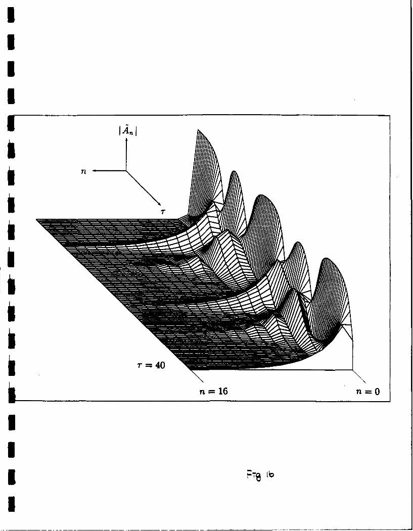
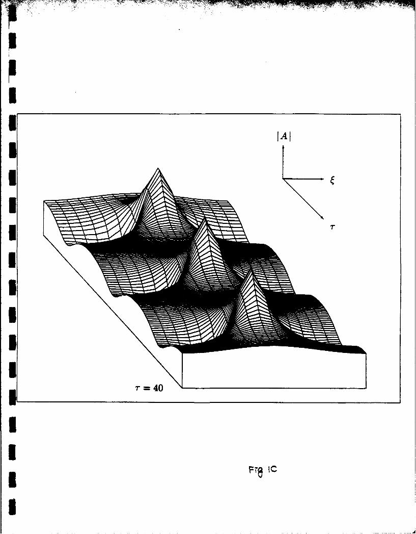
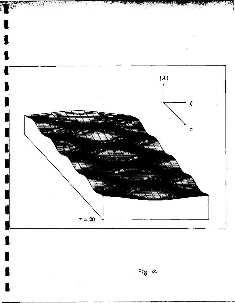
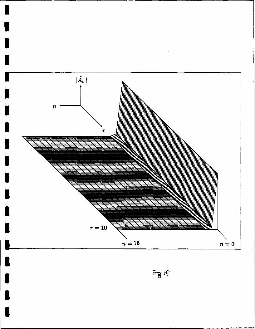
Fig. 1 illustrates the evolution of the Stokes wave (67) for zero viscosity when subject to

the modulation described by (152). Evolution of the envelope amplitude I A(t, r) I is shown in

Fig. la, c, and e, whereas the magnitude of each Fourier coefficient I A,(r) I (n = 0, 1, 2,...) is

plotted in Fig. Ib, d, and f. Since IA,, I is symmetric about n = 0 due to (152), the evolution

for negative n is deleted for clarity. The perturbation wavenumber I = 1 corresponds to complex

recurrence (Fig. la, b); I = 2 corresponds to the maximum initial growth rate and simple

recurrence (Fig. Ic,d). These figures agree with the results of Yuen & Ferguson (1978) and

Weideman & Herbst (1987), who provide detailed explanations. For the simple recurrence, the

fundamental (n = 0) and sideband (n = :I) modes are periodic, as can be also seen in Fig. 8.

The higher modes (not shown in Fig. 8), excited due to nonlinear interaction, are not exactly

3 periodic, but they are not dominant at any stage, making the modulation almost periodic in time.

* 30

I

II

I When I lies outside of the instability range (131), a very nearly periodic oscillation is observed

(Fig. le), which is in good agreement with the neutral stability predicted by the linear analysis.

The corresponding Fourier-space solution (Fig. If) shows that none of the higher harmonics is

fl excited and that the sidebands never become dominant.

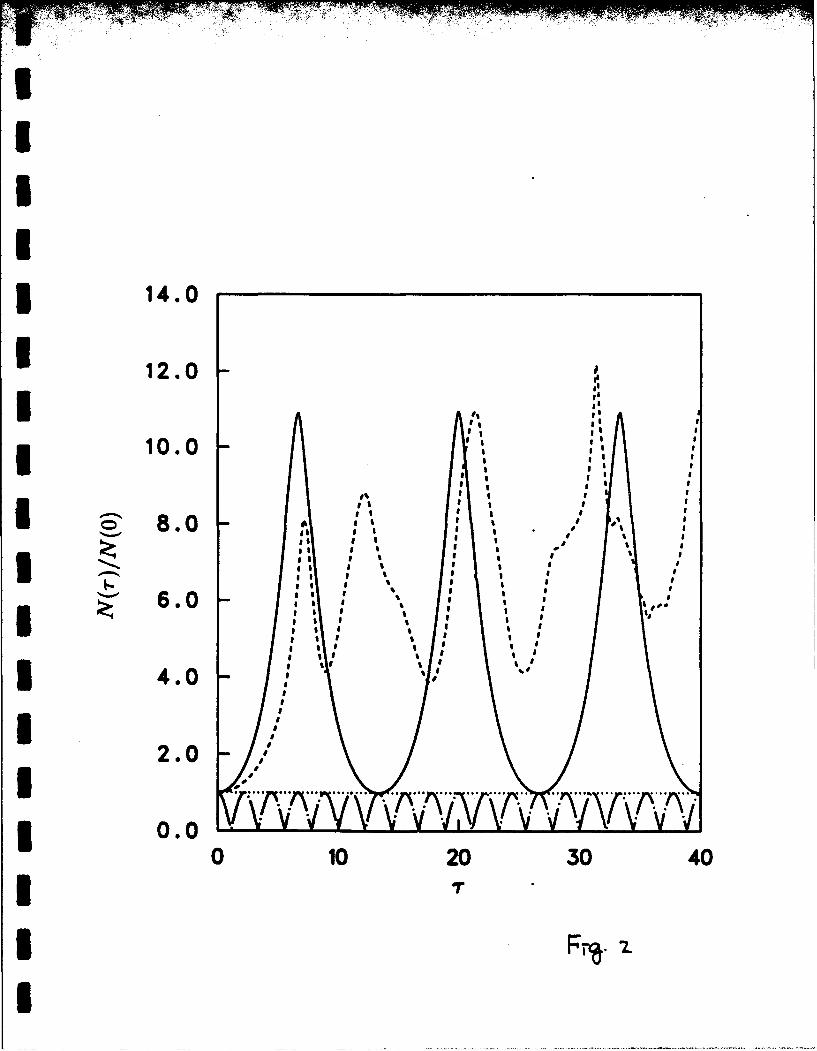
In Fig. 2, the same cases as in Fig. 1 are described using the norm N defined in (123).

3 The behavior for small r is in precise agreement with the linear analysis. The growth rate is a

maximum when I = 2 and decreases as I increases, resulting in larger recurrence periods, until

I it becomes zero for I = 2v2-. When I becomes larger than 2v'2, an oscillation due to neutral

stability is observed, as predicted by the linear analysis. When I decreases from 2, the initial

3 growth rate again decreases, but complex recurrence is observed for I < '2.

Fig. 3 shows the evolution of the slowly varying envelope A for gravity waves with small

Sviscosity. The initial condition and the perturbation wavenumber l are identical to those for the

cases in Fig. 1. Here, the dissipative NLS equation (65) is solved with A = 0.125. In Fig. 3a

3 and 3b, the values of I lie in the instability range, and the initial behavior shows a modulational

instability despite viscous dissipation, which is in agreement with the analysis in the previous

I section for small A. Compared to the corresponding cases in Fig. 1, the spikes are attenuated

at larger times for both the complex and the simple recurrence. In Fig. 3c, the value I = 4 lies

U outside the instability range.

The norm for viscous gravity waves is plotted in Fig. 4. In Fig. 4a, A = 0.125 as in Fig. 3, and

the dependence of the modulation on the pertrbation wavenumber is examined. The amplitudes

of the recurrence are attenuated, as is also seen in Fig. 3, and the spikes are smoother. The value

I = 0.05 lies within the instability range in the inviscid limit (A = 0), but shows decay in Fig. 4a.

3 The effect of A is illustrated in Fig. 4b with I = 2 fixed. As A becomes larger, the amplitude

and period of recurrence decrease; when A = 0.5, we observe monotonic decay. Fig. 4c shows

I the effect of the disturbance amplitude b when I = 2. For small time the growth rate does not

demonstrate amplitude dependence, whereas for larger time the recurrence period increases as

3 b decreases. Other calculations for neutral stability (e.g., I = 4) show that the modulational

*31

I

U

I behavior is hardly affected by changes in b and is almost exclusively dependent on 1, as expected

from the linear analysis.

For capillary-gravity waves with surfactants, the dissipative NLS equation is given by (104).

The coefficient for the dissipation term is independent of the surfact tension T, and the coefficients

for the dispersion and nonlinear terms depend only on T. The term that corresponds to the

3 frequency change in the coefficient for the dissipation term can be absorbed in the carrier wave

and does not contribute to the magnitude of the envelope wave. The qualitative behavior of the

3 modulation is then expected to be identical to that for the gravity waves when T is outside of

the range (149), for the so-called self-focussing type of NLS equation. When T is in the range

1 (149), equation (104) is of the defocusing type. In this case, the long-time modulation exhibits

quite different features from the simple oscillation with constant amplitude and frequency found

3 for neutral stability of the self-focussing type. A discussion of self-focussing and defocussing NLS

equations was given by Peregrine (1983).

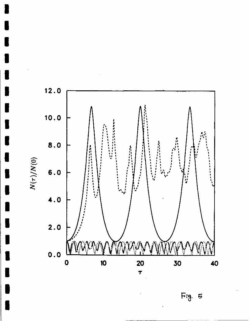
3 Fig. 5 shows the evolution of inviscid capillary-gravity waves (oc = A = 0). The perturbation

wavenumber is chosen as I = 2, and four different values of surface tension are considered. For

I pure gravity waves (T = 0), the maximum growth rate and simple recurrence are observed as

in Fig. 3. For pure capillary waves (T = 1), 1 = 2 lies outside of the instability region, as can

be deduced from (148); thus, an oscillation is observed with constant amplitude and frequency.

For T = 0.1, i = 2 is closer to the lower bound of the instability region I = 0, and so complex

recurrence occurs. The value T = 0.3 lies between 1 - V3/2 and 1/3, and the modulation

shows initial neutral stability, as predicted by the analysis. However, for large time an additional

periodic behavior is observed. The large-scale period increases as I decreases, as can be seen in

Fig. 6a, where I = 1 while the other parameters remain unchanged (T = 0.3 and PC = A = 0). The

corresponding profile for amplitude evolution is given in Fig. 6b. Initially, the behavior is similar

3 to that for neutral stability, but the amplitude then gradually decreases and the frequency starts

to change until the initial envelope disintegrates at about r = 30; still later, the original form

3 of the en' elope is almost completely recovered, near r = 60. Therefore, this phenomenon can

332

- ... . . . . . . -

I

be referred to as recurrence, of a small-amplitude type different from the recurrence related to

Benjamin-Feir instability.

In Fig. 7, we examine the effect of dissipation due to viscosity and a surfactant; A = 0.125,

=I = V5, and 1 = 1/V6. The perturbation wavenumber corresponds to the maximum growth rate

vO- for inviscid pure capillary waves. The norm for the case T = 1 grows to a maximum at twice

its initial value near r = 50 (Fig. 7a). When T = 0.1, the instability with complex recurrence is

observed despite viscous dissipation, whereas for T slightly smaller than 1 - v/!2 (T = 0.1339),

the complex recurrence is suppressed by dissipation, and monotonic decay is observed. For

T = 0.3, a disintegration of the wave envelope is obvious even with viscous damping, as can be

seen clearly in the corresponding evolution profile in Fig. 7b. From Fig. 7, we can also deduce

that the period of the disintegration-recovery has increased from that in Fig. 6 because a smaller

I has been considered.

In all the calculations above, the initial condition used is (152), which corresponds to a

symmetric amplitude modulation. We now consider more general modulations by using (121)

instead, with B1 (0) and B2 (0) not necessarily equal and real as in (152). For simplicity, the

I results for inviscid gravity waves are presented in Fig. 8. Only the dominant fundamental and

the sideband modes are plotted. In all the cases considered, the wavenumber perturbation is

I = 2, so that all exhibit an initial Benjamin-Feir instability followed by simple recurrence. In

Fig. 8a, the given initial condition is identical to that in Fig. la and b, and so the results are

identical. In Fig. 8b, it is obvious that the phase difference changes the modulational behavior

significantly, including the recurrence period. Fig. 8c shows the effect of different initial sideband

amplitudes, here showing an increase in the recurrence period with a decrease in amplitude. In

Fig. 8c, only one of tLe sideband modes is present initially, but subsequent evolution shows that

the other mode is automatically excited to produce the Benjamin-Feir instability. The initially

3 different sideband amplitudes in Fig. 8c become nearly identical, as predicted by Stiassnie &

Kroszynski (1982), but they recover their difference periodically in the subsequent recurrence.

3I 3

U7 Concluding remarks

The methods of multiple scales and matched asymptotic expansions have been used in a

formal derivation of evolution equations for weakly nonlinear viscous water waves. The result is

the nonlinear Schrbdinger equation with an additional linear dissipation term. For both gravity

waves and capillary-gravity waves with an insoluble surfactant, the largest terms in the damping

coefficients are identical to classical linear results. For capillary-gravity waves, nonuniformities

are observed despite dissipation due to the surfactant. Near the second-harmonic resonance,

I a modified set of evolution equations is obtained, which are matched asymptotically with the

nonresonant results. For pure capillary waves, a rescaling of the long-scale free-surface elevation

is required in the presence of surfactants.

The derived evolution equations are solved analytically and computationally to examine the

modulation of infinite wavetrains with sideband disturbances of the Benjamin-Feir type. The

linear analysis shows that in the presence of dissipation the modulation, described by modified

Bessel functions of complex order, has the same initial behavior as the inviscid case but eventually

decays to zero. In the inviscid limit, the instability condition obtained originally by Benjamin

& Feir (1967) is recovered for gravity waves, whereas a stable range of Weber number is found

5 for capillary-gravity waves, which agrees with that obtained by Djordjevic & Redekopp (1977).

In this range, spectral computations show a new type of recurrence not directly related to the

Benjamin-Feir instability.

IThis work was supported by the Program in Ship Hydrodynamics at The University of

Michigan funded by the University Research Initiative of the Office of Naval Research Contract

N000184-86-K-0684, ONR Ocean Engineering Contract N00014-87-0509. The authors acknowl-

3edge Professor J. Boyd for his valuable references and help in computations.

*34

U REFERENCES

IAddison, 1. V. and Schechter, R. S. 1979 An experimental study of the rheological behavior ofsurface films. AIChE Journal, 25, 32-41.

Benjamin, T. B. and Feir, J. E. 1967 The disintegration of wave trains on deep water. J. Fluid.Mech., 27, 417-430.

Craik, A. D. D. 1982 The drift velocity of water waves. J. Fluid. Mech., 116, 187-205.

Davey, A. and Stewartson, K. 1974 On three-dimensional packets of surface waves. Proc. R.Soc. London A, 338, 101-110.

Djordjevic, V. D. and Redekopp, L. G. 1977 On two-dimensional packets of capillary-gravityI waves. J. Fluid Mech., 79, 703-714.

Fermi, E., Pasta, J., and Ulam, S. 1965 Collected papers of Enrico Fermi. Edited bySegre, E. University of Chicago, Chicago, 2, 978.

Garrett, W. D. 1986 ONRL Report C-11-86, 1-17.

Goodrich, F. C. 1960 The mathematical theory of capillarity 1-l1. Proc. Roy. Soc. LondonA, 260, 481-509.

Goodrich, F. C. 1962 On the damping of water waves by monomolecular films. J. Phys. Chem.,66, 1858-1863.

Hasimoto, H. and Ono, H. 1972 Non-linear modulation of gravity waves. J. Phys. Soc. Japan,33, 805.

Joo, S.-W., J. Huh, W.W. Schultz (1989) Capillary-gravity water wave resonance. in preparation.

Lamb H. 1932 Hydrodynamics, 6 h ed. Cambridge University Press.

Levich, V. G. 1941 ZA. Eksperim. Theor. Fiz., 11,340.

Levich, V. G. 1962 Physicochemical Hydrodynamics, Prentice-Hall.

3 Liu, A.-K. and Davis, S. H. 1977 Viscous attenuation of mean drift in water waves. J. Fluid.Mech., 61, 63-84.

Lucassen-Reynders, E. H., and Lucassen, J. 1969 Properties of capillary waves. Adv. ColloidInterface Sci., 2, 347-395.

Lucassen, J. 1982 Effect of surface-active material on the damping of gravity waves: a reap-praisal. J. Colloid Interface Sci., 85, 52-58.

*35

III

Longuet-Higgins, M. S. 1953 Mass transport in water waves. Phil. Trans. R. Soc. LondonA, 245, 535-581.

McGoldrick, L. F. 1970 On Wilton's ripples: a special case of resonant interactions. J. FluidMech., 42, 193-200.

Mei, C.C. 1983 The Applied Dynamics of Ocean Surface Waves, Wiley.

Peregrine, D. H. 1983 Water waves, nonlinear Schrbdinger equations and their solutions. J.Austral. Math. Soc. B, 25, 16-43.

Pereira, N. R. and Stenflo, L. 1977 Nonlinear Schridinger equation including growth and damp-ing. Phys. Fluids, 20, 1733-1734.

Phillips, 0. M. 1966 Dynamics of the upper ocean. Cambridge Univ. Press.

Pliny, 77 A.D. Naturalis Historia. Book ii, Chapter 107, section 234.

Reynolds, 0. 1880 On the effect of oil on destroying waves on the surface of water. Br. As-soc. Rept.; Papers, 1, 409.

Stiassnie, M and Kroszynski, U. I. 1982 Long-time evolution of an unstable waLer-wave train. J.Fluid Mech., 116, 207-225.

Stuart, J. T. and DiPrima, R. C. 1978 The Eckhaus and Benjamin-Feir resonance mechanisms.3 Proc. R. Soc. London A, 362, 27-41.

Unliiata, U. and Mei, C. C. 1970 Mass transport in water waves. J. Geophys. Res., 75, 7611-7618.

Weideman, J. A. C. and Herbst, B. M. 1987 Recurrence in semidiscrete approximations of thenonlinear Schr~dinger equation. SIAM J. Sci. Stat. Comput., 8, 988-1004.

Whitham, G. B. 1967 Nonlinear dispersion of water waves. J. Fluid Mech., 27, 399-412.

Yuen, H. C. and Ferguson, W. E. 1978 Relationship between Benjamin-Feir instability and re-currence in the nonlinear Schr6iinger equation. Phys. Fluids, 21, 1275-1278.

Zakharov, V. E. 1968 Stability of periodic waves of finite-amplitude on the surface of deep fluid.J. Appl. Mech. Tech. Phy., 9, 190-194.

* 36

I

77 7

I LIST OF FIGURES

Figure 1. Evolution of modulations for inviscid gravity waves (A = 0) when the amplitude per-

turbation b is 0.1: a) I = 1, b) I = 1 Fourier space, c) I = 2, d) I = 2 Fourier space, e) i = 4, f)

3 1 4 Fourier space.

Figure 2. Evolution of modulations for gravity waves expressed by N(r)/N(0) for I = 1

( 1), = 2 (-), 1 = 2V ( ...... ), and = 4(-.-).iFigure 3. Evolution of modulations for gravity waves with small viscosity (A = 0.125): a)

1 =1, b) I=2, c) I=4.

I Figure 4. Evolution of modulations for gravity waves when: a) A = 0.125 and b = 0.1 are

fixed, and the perturbation wavenumber varies for I = 0.05 ( ...... ), 1 = (---- ), I = 2 (- ),

and 1 = 4 (- --) b) 1= 2 and 6 = 0.1 are fixed, and the viscous dissipation varies for A = 0

(-), A = 0.125 ( --- ), A = 0.25 (- . -), A = 0.5 ( ...... ), and A= 1 (---) c)1=2and

A = 0.125 are fixed, and the amplitude perturbation varies for b = 0.01 (- ), b = 0.1 (1 . -

Sb= 0.2 (- -),and b = 0.3 ( ......

3 Figure 5. Evolution of modulations for inviscid capillary-gravity waves (A = x 0) when

the perturbation wavenumber I = 2 and the Weber number is chosen as T = 0 (-), T = 0.1

3 (- - -), T= 0.3 (- . -), and T = 1 ( ...... ).

5 Figure 6. Evolution of modulations for inviscid capillary-gravity waves (A = = 0) when

the perturbation wavenumber I is 1 and the Weber number T is 0.3 expressed by: a) N(r)/N(O)

U b) I A(t, r)I.

3 Figure 7. Evolution of modulations for capillary-gravity waves in the presence of viscosity

*

I

!I

(A = 0.125) and surfactant (ic = V2-) when the perturbation wavenumber I = 1V/ and the

Weber number is chosen as: a) T = 0.1 (- ), T = 0.1339 ( .... ), T = 0.3 (- -), and

T= 1 ( ...... )b)T=0.3.

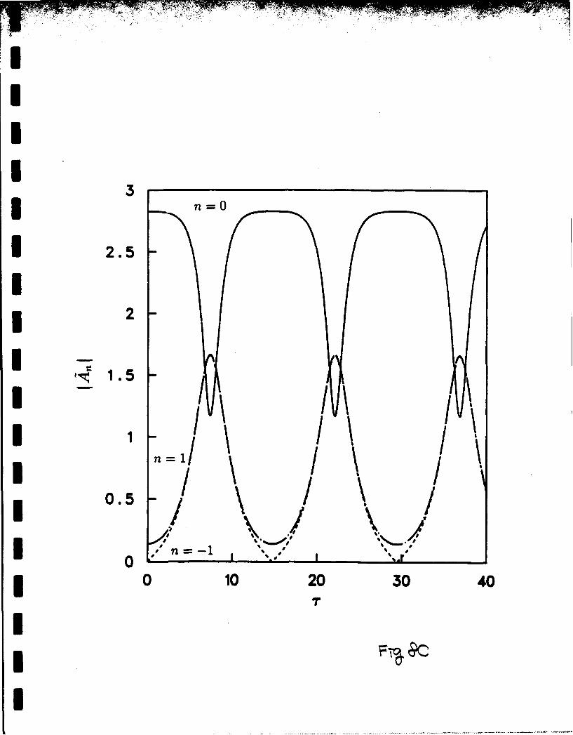
Figure 8. Evolution of dominant Fourier modes (n = 0 and +1) for inviscid gravity waves

I when I = 2. The initial sideband amplitudes are represented by: a) B1 = 0.05 and B2 = 0.05, b)

B, =0.05 and B2 = 0.05 i, c) B1 = 0.05 and B2 =0.

IiII

IiIII$I

JAI

40.

I0

map* 40

nI6

77wl; 3 ' i- 7FM

II

I IAn I

a4n 16nn

S n= 16

I

UA

II

JA

U

U

I nn

-I -----I-I

n n1 6 0

Ii

IIII3 14.0

12.0

10.0a

| a'

Z-3 a.

a o o - !|~ ItmliiiI I'

6. 0 1 poll

SI a

a 5I| a

gI g

I a I

4 .0 A 4

a q I

0.0 1' v ""at a a'

0 10 20 30 40

atFr a7aa-I a -,a.I a

I

UIII

Al

IIII

JAI

.b

I

I

rI'-4

I

JAI

NOBE

I1

IUI.

* 10.0

U* 8.0

IU

* 4.0a a

4.0 ,

* 2.0I tII

0.020 o,20304

i

I

I 12.0

iI 10.0-

* 8.0 - ,

a i

*a / "ao :a /\

I a t It

40 10 20304a a r,

15.

3 25.0

* 20.0

0 105.03 4

* ~ 10.0

i

IiU

II 12.0

I , i* 80

iIi

,i:I i aI s *II Ia ~ I I I a "

all V i i~ i ia i I 5,

a II V I

Si I 1 I I IU a I Ia

I aI

II

*400 ' .

I ,rI t5

U#

II

I

3 1.6

I 1.4 -

3 1.2I1.0

3 > 0.8

* 0.6

3 0.4II 0.2

II 0.0 i0 20 40 60 80

I

JAI

IN N

'r80

I6

mMw II

Imm

* 5.0

4.0 -

I3.0 -

m* 2.0

1.0

0. 0 V0 20 40 60 80

I

IIII

I*

V

aaI

U0

1.

I 1.5

0I02 04

1 /I / \

I

I

II

2.5II n-O

2

I1.5

I

0.5

I0 10 20 30 407"

- Fi. 9I

2.5~

-- I

I

I . ~~ _ __ __ __ _

i3I n-o

I 2.5

II 2 -

n- -I/ \, 1~ / \,

I I xII I

I