The University of Manchester Research

Itchy Feet vs Cool Heads: Flow of Funds in an Agent-basedFinancial MarketDOI:10.1016/j.jedc.2015.12.002

Document VersionAccepted author manuscript

Link to publication record in Manchester Research Explorer

Citation for published version (APA):Jan Palczewski, Schenk-Hoppe, K., & Tongya Wang (2016). Itchy Feet vs Cool Heads: Flow of Funds in an Agent-based Financial Market. Journal of Economic Dynamics and Control, 53–68.https://doi.org/10.1016/j.jedc.2015.12.002

Published in:Journal of Economic Dynamics and Control

Citing this paperPlease note that where the full-text provided on Manchester Research Explorer is the Author Accepted Manuscriptor Proof version this may differ from the final Published version. If citing, it is advised that you check and use thepublisher's definitive version.

General rightsCopyright and moral rights for the publications made accessible in the Research Explorer are retained by theauthors and/or other copyright owners and it is a condition of accessing publications that users recognise andabide by the legal requirements associated with these rights.

Takedown policyIf you believe that this document breaches copyright please refer to the University of Manchester’s TakedownProcedures [http://man.ac.uk/04Y6Bo] or contact uml.scholarlycommunications@manchester.ac.uk providingrelevant details, so we can investigate your claim.

Download date:03. Jan. 2020

Itchy Feet vs Cool Heads: Flow of Funds in an

Agent-based Financial Market∗

Jan Palczewski a

Klaus Reiner Schenk-Hoppe b

Tongya Wang c

November 17, 2015

Abstract

Investors tend to move funds when they are unhappy with their cur-rent portfolio managers’ performance. We study the effect of the sizeof this flow of funds in an agent-based model of the financial market.The model combines the discrete choice approach from agent-basedmodelling, where all capital is mobile, with the evolutionary financeframework where all growth is endogenous. Our results show that, ifinvestors exhibit recency bias in evaluating portfolio managers’ perfor-mance, even a small amount of freely flowing capital has a huge impacton the market dynamics and the survival of noise traders. We also findthat investors’ intensity of choice is a driving force for excess volatilityand extreme price movements when the size of the flow of funds islarge.

Keywords: Portfolio management; agent-based financial market; evolution-ary finance; flow of funds.JEL classification: D53; G18; C63.

∗Part of this paper, which grew out of Chapters 3 and 4 of TW’s PhD Thesis [46], waswritten during the authors’ visit to the Hausdorff Research Institute for Mathematics atthe University of Bonn in the framework of the Trimester Program Stochastic Dynamicsin Economics and Finance.

aSchool of Mathematics, University of Leeds, United Kingdom. E-mail:j.palczewski@leeds.ac.uk.

bEconomics, School of Social Sciences, University of Manchester, United Kingdom,and Department of Finance, NHH–Norwegian School of Economics, Norway. E-mail:klaus.schenk-hoppe@manchester.ac.uk.

cSaıd Business School, University of Oxford and Centre for Advanced Studies in Fi-nance, University of Leeds, United Kingdom. E-mail: tongya.wang@sbs.ox.ac.uk. (Cor-responding author).

1

1 Introduction

Providers of portfolio management services chase excess returns in the assetmarket as well as new money from investors. These are two closely inter-twined goals: A portfolio manager who outperforms many of their peerstends to see exogenous growth through the inflow of money from new andexisting clients as well as endogenous growth through returns on the capitalemployed.1

The exogenous growth of investment funds through the inflow (or out-flow) of money is at the heart of much of the agent-based literature onfinancial markets, see, e.g., the textbook Hommes [26] and the surveysHommes [25], Chiarella et al. [14], Hommes and Wagener [28], and Let-tau [35]. These models are populated by a small number of different in-vestment styles and an infinite number of clients who move money betweenthe available styles based on differences in performance, measured, e.g., as aweighted average of realised excess returns. To capture the impact of port-folio managers’ performance on the reallocation of investors’ money, thisliterature generally employs a discrete choice model. In the absence of bor-rowing/lending constraints, strategies can lever their positions without limitand, as a result, have a disproportional short-term price impact. As moneyunder management does not matter for a fund’s asset allocation, asset pricesare driven by the dynamic of expectations about future excess returns whichcan result in excess volatility with consistent deviation of asset prices fromfundamental values.

Endogenous growth through investment returns and its consequences forasset prices in evolutionary, agent-type finance models have been studied inAmir et al. [1] and Evstigneev et al. [20, 21]. These models contain a smallnumber of portfolio managers who aim to grow funds under managementbut do not face client attrition. The price impact of investors is proportionalto their funds, and there is no leveraging. A main result in that literatureis that there is only one asset price system that is stable (in the long term)

1See, e.g., the survey papers by Constantinides, Harris and Stulz [16, Chapters 14, 15,21 and 22] and Anderson and Ahmed [2].

2

against the entry of new investment styles. This benchmark price system isgiven by the expected value of the discounted sum of relative asset payoffs(a generalisation of the Kelly investment rule).

This paper combines exogenous and endogenous growth of funds in onemodel. Investors can move their funds between portfolio mangers with dif-ferent styles, but the total amount of freely flowing capital is a model pa-rameter. There is no leveraging: the more funds a portfolio manager holds,the stronger its price impact. By varying the size of the flow of funds in thismodel, we can explore the relative importance of the two different sourcesof growth for asset price dynamics.

The exogenous amount of freely flowing capital in each time period canbe interpreted as the average client’s degree of patience. If the proportionis small, most investors keep cool heads and tend to stick with their port-folio manager even during long periods of poor performance. On the otherhand, when this amount is large, clients have itchy feet and tend to desertan under-performing portfolio manager quickly. There is a substantial dif-ference between this approach to modelling the flow of funds and the usualdiscrete choice formula in agent-based models of financial markets: we cancontrol the amount of freely flowing capital and thus the general degree ofimpatience in the market by varying the level of client attrition. The dis-crete choice formula is used however to model the destination of the freecapital. The idea of modelling non-switching and switching investors is sim-ilar to the one of Dieci et al. [18] with the same motivation. However, theirmodel is based on the framework of Brock and Hommes [8, 9] where thebudget effect and the interdependence between wealth and prices are left inthe background. An exception is Bottazzi and Dindo [5] who study agentswith decision rules that can be driven by past prices.

The agent-based part of the model presented here is most closely relatedto that part of this literature that forbids short-selling: Anufriev and Dindo[3], LeBaron [30, 31, 32, 33] and Levy, Levy and Solomon [36, 37, 38, 39]. Inthese papers the budget constraint limits the potential market impact of thedifferent investment styles. This is in contrast to the models where unlimitedpositions are possible (e.g. Chiarella, Dieci and Gardini [13] and Brianzoni,

3

Mammana and Michetti [7]) and those where asset prices are driven onlyby funds’ expectations about future returns (e.g. Brock and Hommes [8, 9],Gaunersdorfer and Hommes [23]).

The evolutionary finance part of the model extends Evstigneev et al. [22]by adding an explicit mechanism that reallocates a certain proportion offunds between the different portfolio managers. In these models leverage isexcluded and therefore the available budget constrains the positions that afund manager can take on as well as their market impact. The hybrid modelpresented here bridges the gap between the agent-based and the evolutionaryapproach. It can be used as a powerful tool to obtain insightful resultsregarding the feedback loop between the exogenous flow of funds with budgeteffect, the endogenous growth of wealth, and the price dynamics.

Our paper is also closely related to inquires into the interaction of passiveand active learning dynamics, as defined in LeBaron [34]. Passive learn-ing refers to the market force by which wealth accumulates on investmentstrategies which have done well (in relative terms). Active learning refers tothe switching behaviour by which investors reallocate wealth into strategieswhich have performed well in the past. As LeBaron points out, althoughboth learning types and their consequences on the price dynamics have beenextensively studied in isolation, the interaction between the two remainslargely unexplored.

We are particularly interested in the impact of the size of the flow offunds on systematic deviations of prices from fundamental values as wellas on excess volatility. This inquiry has both theoretical as well as practi-cal aspects. Under the discrete choice model, all capital is ready to moveat any time. In evolutionary finance models, all funds stay with the sameportfolio manager. In reality however clients’ behaviour fits neither descrip-tion. Investors do not continuously monitor the performance of all portfoliomanagers and move funds at all times, nor do they ignore performance andnever switch to managers with superior performance. As stressed by Dieciet al. ([18], p. 520): “Empirical evidence has suggested that, facing differenttrading strategies and complicated decision, the proportions of agents relyingon particular strategies may stay at constant level or vary over time.”.

4

Since our model separates the clients’ allocation decision from the amountof freely flowing capital, we look more closely into the relation between be-havioural aspects, such as differences of opinions, recency bias in perfor-mance evaluation, conservatism bias (e.g., Edwards [19]) and rational herd-ing, and the model parameters. We also explore the impact of some of thesebehavioural phenomena on the asset price dynamics.

The next section introduces the general framework of the hybrid modeland provides a specification with three investment styles. The detailed nu-merical study of the model is provided in Section 3. Section 4 concludes.All proofs are collected in an appendix. The software and data are availableat www.schenk-hoppe.net/software/flow-of-funds/.

2 Model

2.1 General framework

We consider a financial market in which K ≥ 1 risky assets and one risk-free asset are traded at discrete points in time t = 0, 1, .... Risky assetsk = 1, ...,K pay dividends Dt,k ≥ 0. (Dt,1, ..., Dt,K) is a stationary stochas-tic process with

∑Kk=1 Dt,k > 0 and EDt,k ≡ Dk < ∞. Risky assets are in

constant positive supply, normalised to 1, and their prices Pt,k will be deter-mined through short-run equilibrium of supply and demand. The risk-freeasset k = 0 has a constant price Pt,0 = 1 and pays a constant interest r > 0per period.

There are I ≥ 1 portfolio managers (funds) in the market which managewealth on behalf of their clients. The portfolio held by fund i at time t isdenoted by a vector θi

t = (θit,0, θ

it,1, ..., θ

it,K) representing the number of units

of each asset. The quantity θit,k is given by

θit,k = (1− c)

λit,kW

it

Pt,k, k = 0, 1, ...,K, (1)

where W it is the wealth managed by fund i at time t, 1 − c ∈ (0, 1) is the

fraction of wealth reinvested in every period (the remainder is, e.g., used

5

for management fees or clients’ consumption), and λit = (λi

t,0, ..., λit,K) is

a vector of investment proportions with λit,k ≥ 0 and

∑Kk=0 λi

t,k = 1. Weassume that λi

t can depend on past observations of dividends, asset pricesand investment strategies up to time t−1. These strategies can also exhibitadditional, inherent randomness as long as it is independent from dividendsand other strategies at times t, t + 1, ....

The value of fund i’s holdings at the end of investment period [t, t + 1)is equal to

V it+1 =

K∑k=1

[Pt+1,k + Dt+1,k]θit,k + (1 + r)θi

t,0. (2)

Equation (2) describes the endogenous change in an investment fund’s wealth,i.e., the gains or losses of a fund’s wealth due to the asset returns.

The exogenous change of wealth under management is caused by clientsmoving investments between the different funds at the end of each period.The decision to reallocate investments is driven by observed performance offunds. We assume that each time period a fraction β ∈ [0, 1] of all invest-ments is allocated according to some performance measure. The remainingfraction 1− β stays with the fund where it is currently invested. Formally,

W it+1 = (1− β)V i

t+1 + qitβVt+1, (3)

where Vt+1 =∑I

i=1 V it+1 is the aggregate wealth under management of all

funds and qit, i = 1, ..., I, are proportions (qi

t ≥ 0,∑

i qit = 1) that depend on

the funds’ performance up to time t. Equation (3) says that, after clients’completed their reallocation of funds, the actual wealth W i

t+1 managed byan investment fund i at the beginning of the period [t + 1, t + 2), consists oftwo parts: the wealth that stays with this fund, (1− β)V i

t+1, and the (new)wealth received by this fund, qi

tβVt+1. The value of W it+1 is the budget of

fund i which is available for investment at time t + 1. The parameter β

allows to control the maximum amount of capital that can flow between thefunds. In contrast to other agent-based models, for each $1 of wealth, only$β will be reallocated.

If clients cannot move investments between funds (β = 0), equation (3)

6

implies that each fund’s budget W it+1 is equal to the value V i

t+1 of its timet+1 holdings. Then wealth under management can only grow endogenously.If clients can move investments between funds (β > 0), the actual budgetW i

t+1 is affected by the exogenous flows of wealth. Depending on the signof W i

t+1 − V it+1, the net inflow or outflow of wealth into a fund i is given by

β(qitVt+1 − V i

t+1

).

Market clearing for each risky asset requires∑I

i=1 θit,k = 1, k = 1, ...K,

which is equivalent to

Pt,k = (1− c)I∑

i=1

λit,kW

it . (4)

Since the price of the risk-free asset is 1, θit,0 = (1 − c)λi

t,0Wit is equal to

the amount invested in that asset. With specification (3), we can write thedynamic of wealth under management as

V it+1 =

K∑k=1

λit,k[(1− β)V i

t + βqit−1Vt]

〈λt,k, (1− β)Vt + βqt−1Vt〉×(

(1− c)[(1− β)〈λt+1,k, Vt+1〉+ β〈λt+1,k, qt〉Vt+1

]+ Dt+1,k

)+(1 + r)(1− c)λi

t,0

[(1− β)V i

t + βqit−1Vt

],

with i = 1, ..., I, where 〈x, y〉 =∑

i xiyi denotes the scalar product, and(dropping the time index) V = (V 1, ..., V I)T ∈ RI

+, λk = (λ1k, ..., λ

Ik)

T ∈ RI+,

and q = (q1, ..., qI)T ∈ RI+ with R+ denotes the set of non-negative real

numbers. Equivalently, using vector notation,

Vt+1 = Θt

[(1− c)

[(1− β)Λt+1 + βΛt+1qt1

]Vt+1 + Dt+1

]+(1 + r)(1− c)∆λt,0

[(1− β)Vt + βqt−11Vt

], (5)

where Λ = (λik) ∈ RK×I

+ , 1 = (1, ..., 1) ∈ RI , D = (D1, ..., DK)T ∈ RK+ , and

∆λ0 ∈ RI×I+ has entries λi

0 on the diagonal and zero otherwise. Denoting

7

Wt = (W 1t , ...,W I

t )T ∈ RI+, the portfolio matrix Θ ∈ RI×K

+ is given by

Θik =ΛkiW

i

(ΛW )k=

Λki[(1− β)V i + βqiV ][Λ((1− β)V + βq1V

)]k

.

Conditions ensuring that the dynamic (5) is well-defined are providedin the following result which is proved in Appendix A. Here RI

++ = {a ∈[0,∞)I :

∑Ii=1 ai > 0} denotes the set of non-zero vectors with non-negative

coordinates.

Proposition 2.1. For any Vt ∈ RI++, there is a unique Vt+1 ∈ RI

++ solving(5) provided there is at least one fund i with V i

t > 0, which is fully diversifiedin risky assets, i.e., λi

t,k > 0 and λit+1,k > 0 for all k ≥ 1. If β = 1 it is

further required that qit > 0.

The proof of this result also yields an explicit expression of the dynamic:

Vt+1 =[Id− (1− c)Θt

((1− β)Λt+1 + βΛt+1qt1

)]−1×[

ΘtDt+1 + (1 + r)(1− c)∆λt,0

[(1− β)Vt + βqt−11Vt

]](6)

with Id the I-dimensional identity matrix.2 Using this result, each fund’sbudget W i

t+1 can be computed by inserting (6) into the specification (3).

2.2 Benchmark

Assume there is one risky and one risk-free asset, and a single portfoliomanager. Then the dynamic (6) reduces to

Vt+1 =Dt+1 + (1 + r)(1− c)λt,0Vt

1− (1− c)λt+1,1(7)

and the risky asset’s price is

Pt+1 = (1− c)λt+1,1Vt+1. (8)

2Setting β = 0 in (6), one obtains the dynamic studied in Evstigneev et al. [22].

8

One therefore finds the recursive equation

Pt+1 =(1− c)λt+1,1

1− (1− c)λt+1,1

[Dt+1 + (1 + r)

1− λt,1

λt,1Pt

]. (9)

Let the dividend (Dt) be a stationary process with a finite variance.Then we have the following result (its proof is given in Appendix A):

Proposition 2.2. Let c ≥ r/(1 + r) and assume that λt,1 ≡ λ ∈ (0, 1] is aconstant and σ2 = V ar(D0) < ∞.

(i) The process

P ∗t = b

0∑n=−∞

a−nDt+n (10)

witha = (1 + r)

(1− c)(1− λ)1− (1− c)λ

, b =(1− c)λ

1− (1− c)λ(11)

is a stationary solution to the dynamics (9).(ii) For each P0 ≥ 0, the price process Pt converges a.s. to the path (P ∗

t )in the following sense

limt→∞

|Pt − P ∗t | = 0 a.s.

(iii) The expectation and variance of the stationary solution are as fol-lows

EP ∗t =

b

1− aED0 =

b

1− aD, V ar(P ∗

t ) =b2σ2

1− a2.

Interpretation. Suppose c = r/(1 + r). Then the above result showsthat the price of the risky asset converges to a stationary process (P ∗

t ).Moreover the expectation of this process is equal to the fundamental value:

E(P ∗t ) =

D

r. (12)

This result holds regardless of the portfolio manager’s investment strategyλ as long as it is a constant. The volatility of the price process (P ∗

t ) however

9

depends on the specific strategy. For c = r/(1 + r), one finds that

V ar(P ∗t ) =

σ2λ/r

r + (2 + r)(1− λ).

In the particular case σ = 0, the price process becomes deterministic. Thenthe condition c = r/(1 + r) implies that the fundamental value is a uniquefixed point of the price process.

To have the fundamental value as an equilibrium benchmark, we setc = r/(1 + r) throughout the remainder of the paper.

2.3 Model specification

We focus on the model with one risky and one risk-free asset. The investmentproportion for the risky asset can then be expressed by a single numberλt ∈ [0, 1]. Given λi

t, fund i invests according to (1 − λit, λ

it). We assume

that dividends are i.i.d. with truncated normal distribution N (µ, σ)+, seeAppendix B for details on the implementation.

Investment strategies of portfolio managers. We consider threeinvestment strategies, each followed by one portfolio manager: fundamental,trend-following and noise trading. These investment styles are the mostcommonly studied in the heterogeneous agent-based literature, see, e.g.,Hommes [25, 26]. All three strategies are based on subjective forecastsof expected cum-dividend excess returns. For each investment style, theforecast Ft of the excess return of risky over the risk-free asset between thecurrent and the next period is computed as follows.

The fundamental fund forecasts price reversal to the fundamental value:

FFt =

D/r + D − Pt−1

Pt−1− r =

[D/r

Pt−1− 1]

(1 + r).

Here D is the expected dividend payment, and D/r the risky asset’s funda-mental value.

The trend-chasing fund interpolates the trend observed in the last L

10

periods to forecast future excess return:

F Tt = (1/L)

L∑j=1

Pt−j + Dt−j − Pt−1−j

Pt−1−j− r.

The noise-trader fund makes randomly revised forecasts according to anAR(1) process:

FNt = δFN

t−1 + εξt, ξt ∼ N(0, 1) (13)

with constants δ ∈ (0, 1) and ε > 0.Given a forecast Ft, the demand of each fund at time t is determined

by a demand function that maps Ft into an investment proportion λt. Toensure the dynamics of funds’ wealth is well-defined (Proposition 2.1), thevalue of λt has to be bounded by zero and one, i.e., there is no leverage orshort-selling. On the other hand, we want agents’ portfolio decision to beproportional to changes in their forecasts.

A natural candidate for the demand function is a symmetric S-shapedsmooth function whose values are in the interval (0, 1) and where the slopeat zero is controlled by a parameter. Similar to Lebaron [29, 30, 31] andChiarella, Dieci and Gardini [12, 13], we adopt a sigmoid demand functionto determine the investment proportions of each fund type with respect totheir forecasts of excess returns.3 The value of λt is given by4

λt = (1/π) arctan(αFt) + 1/2. (14)

The investment proportions in the risk-free and the risky asset are givenby (1 − λt, λt). The parameter α ∈ (0, 1) describes how strongly the fundreacts to perceived future excess return. Formula (14) guarantees that for

3LeBaron argues that, in a model with heterogenous agents, deriving optimal demandfrom utility maximisation requires an agent to be informed about the states of other agentswhich is unrealistic. Agents’ demand is therefore modeled with a simple rule based ona sigmoid function. Chiarella et al. use sigmoid functions to capture agents’ demand tocapture expectations of an increase in market risk when the absolute value of expectedexcess return rises, e.g., during periods of booms or crashes.

4The trigonometric function arctan takes values in (−π/2, +π/2). Hence dividing byπ and adding 1/2 gives values between 0 and 1.

11

any forecast the fund takes long positions in both risk-free and risky assetbecause λt ∈ (0, 1). The S-shaped demand curve captures a simple butgeneral heuristic in investment — investors tend to increase (or decrease)diminishingly their investments in the risky asset along with the increase(or decrease) in perceived future excess return. Different to models whereinvestment proportions are derived from utility maximisation (e.g. Levy,Levy, and Solomon [39] and Chiarella and He [15]) with a purpose to char-acterise agents’ optimal behaviour, the demand function (14) used here is tofacilitate behaviourally the modelling of the three typical investment stylesmentioned above5.

Flow of clients’ money. We follow Brock and Hommes [9] in assum-ing that investors reallocate the wealth that is withdrawn from funds inproportions

qit =

exp(γf it )

I∑j=1

exp(γf jt )

, (15)

where f it is the sum of discounted realised log returns of fund i:

f it = log(φi

t) + ρf it−1 (16)

with

φit =

V it

(1− c)W it−1

. (17)

Here φit is fund i’s realised return between period t− 1 and t, and ρ ∈ [0, 1]

is the discounting factor. The parameter γ ≥ 0 measures clients’ sensitivity5Levy, Levy, and Solomon [39] and Chiarella and He [15] may represent two typical ap-

proaches for solving investment proportions via maximising CRRA type utility functionsin agent-based models. Both approaches require ad-hoc assumptions to restrict invest-ment proportions between zero and one. The former solves investment proportions andthe market clearing price simultaneously by a numerical search procedure. This method isequivalently to assume that each agent in the market knows others’ investment strategiesso that all agents are able to compute the current market clearing price. The latter de-rives investment proportions based on a closed-form solution to utility maximisation withparticular assumptions on the wealth dynamics. The resulting investment proportionsdepend linearly on expected excess returns. A negative expected excess return will causeagents to withdraw immediately all investments from the risky asset regardless of theirprevious positions.

12

to differences in observed performance of portfolio managers.

A key feature of (15) is the heterogeneity of clients’ choices. For everyparameter value γ ∈ [0,∞), some positive (gross) amount of wealth flowsto each investment fund. But the actual net flow is dependent on all funds’performances. A crucial issue for the model dynamics is therefore whichcondition implies an increase or decrease in the proportion qi of a fund i

between time t and t + 1. A short discussion of this neglected issue follows.Let us look at the sign function sgn(qi

t+1−qit) where a positive (negative)

sign of qit+1 − qi

t refers to a net increase (decrease) of wealth. Define theimprovement of an investment fund’s strategy i = 1, ..., I during a timeinterval [t, t + 1] as:

∆it+1 = f i

t+1 − f it ,

and the average improvement of all investment funds’ strategies during thetime interval [t, t + 1] as:

∆t+1 =1I

I∑i=1

∆it+1.

The condition which triggers the increase or decrease in qi can be char-acterised in the following proposition.

Proposition 2.3. For each investment fund’s strategy i = 1, ..., I, the signof qi

t+1 − qit is determined by the sign of ∆i

t+1 − ∆t+1:

sgn(qit+1 − qi

t) = sgn(∆it+1 − ∆t+1).

This result shows that clients have a tendency to choose funds whose im-provements are higher than the average level. Note that a fund j which hasthe highest performance measure f j

t+1 at time t+1 does not necessarily havea higher improvement ∆j

t+1 than the average level. The ‘best performed’fund type j may lose clients at time t + 1 if its improvement ∆j

t+1 falls be-low the average. Such a property reveals that clients with itchy feet holda different interpretation for the performance measure: the improvement of

13

an investment fund. Itchy-feet clients are sensitive to the improvements offunds and thus liable to overreact to changes in performance when choosingbetween funds.

Proposition 2.3 further provides insights into the difference between thetwo widely studied type-switching mechanisms: The discrete choice ap-proach as described by equation (15) and the replicator dynamics used inevolutionary game theory. Branch and McGough [6] apply the later in theframework of Brock and Hommes [8]. They find that the replicator dynamicsimplies that the proportion qi

t for agents who choose a predictor i at time t

will increase (decrease) at time t+1 if the value of predictor i’s performancemeasure is higher (lower) than the value of the average performance measureacross all available predictors. Therefore, under the replicator dynamics, theuse of some predictors will cease over time. But according to Proposition 2.3under the discrete choice approach, agents’ choice of predictors is sensitiveto the improvement in predictors’ performance measures rather than the dif-ference between predictors’ performance measures. Hence even predictorsthat are dominated can survive if their performance is volatile enough.

2.4 Discussion of behavioural aspects

Clients’ psychology may play an important role in the choice of investmentfunds, especially when clients are boundedly rational. By linking to thebehavioural finance literature, we explain and discuss some psychologicalelements and behavioural phenomena which are covered by the model.

Differences of opinion. The foundation for the switching mechanism(15) is the randomized discrete choice framework of McFadden [41], whereasBrock and Hommes [8, 9] utilised it in dynamic equilibrium models of finan-cial markets to study the adaptation of investors. In discrete choice studies,not all agents necessarily choose the option, here the investment fund, whichis indicated (by the model) to have the highest performance measure. Such aphenomenon corresponds to the case of γ ∈ [0,∞) in (15). The finite valueof γ implies that agents are heterogeneous in making choices of availableoptions. The reason for such heterogeneity of agents is explained by McFad-

14

den [41] as unmodeled idiosyncratic components in agents’ utility function orrandomness in agents’ preferences, while Brock and Hommes [8, 9] attributethis heterogeneity to agents’ bounded rationality.

Our model characterises various types of differences of opinion amonginvestors. First, the differences in prior beliefs is modelled by the set ofdifferent fund types. The presence of cool-head investors may reinforce thistype of differences of opinion. Second, the switching mechanism (15) withγ ∈ [0,∞) is able to capture the differences of opinion in fund selection andthe phenomenon that clients hold different interpretations of the public per-formance measure (16) of each fund type. When γ ∈ [0,∞), each itchy-feetinvestor can be thought as having a private measurement or interpretationfor the performance of each strategy. As revealed by Proposition 2.3, theimprovement of strategy ∆i

t = f it − f i

t−1 can be regarded as an exampleof this kind of private measurement or interpretation for the performanceof each strategy. This may lead to the phenomenon that some itchy-feetinvestors choose fund types according to the value of public performancemeasure, i.e., the value of f i

t , while some may make their choices based onthe value of improvement of each fund type, i.e., the value of ∆i

t.In this switching mechanism, the distribution of clients’ investments

among different fund types becomes more (or less) diversified when the valueof γ becomes low (or high). For this reason, the degree of differences of opin-ion among investors in strategy selection can be measured by the value ofγ ∈ [0,∞). A lower (or higher) value of γ corresponds to a higher (or lower)degree of differences of opinion.

Conservatism bias and rational herding. Different degrees of dif-ferences of opinion in strategy-switching may represent different behaviouralphenomena, such as conservatism bias and rational herding. Edwards [19]identified the phenomenon of conservatism which describes that people re-act conservatively to new information, and they are slow to change an es-tablished view. In the context of performance-driven fund flows, a microlevel foundation for conservatism is that switching investors tend to be lesssensitive to the evidence of the performance of each strategy. A resultingmanifestation on the macro level is that the average amount of the net flows

15

of wealth is low. Such a phenomenon can be captured when the value of γ

is low.6

Rational herding refers to the tendency that investors to react to infor-mation about the behaviour of other investors. According to Bruce [11],rational herding happens because some investors believe others can performbetter than themselves, therefore they follow or mimic others’ behaviour.Such a phenomenon can be captured when the value of γ is high, sincea high value of γ implies that investors are less conservative and a largeproportion of investors will switch fast to the best performing investmentstrategy.

In our model, the market impact of the differences of opinion in strategyselection and its related behavioural phenomena can be studied by exploringhow different values of γ in (15) affects the market dynamics.

Recency bias. This cognitive bias is related to the way that individ-uals digest information. Recency bias refers to the tendency of individualsto assign more importance to more recent information compared to thosefarther in the past. In the behavioural finance literature, recency bias havebeen widely studied in relation to asset valuation and evaluation of funds’performance. For example, as stated in Pompian ([43], p. 216): “one ofthe most obvious and most pernicious manifestation of recency bias amonginvestors pertains to their misuse of investment performance records for mu-tual funds and other types of funds. Investors track managers who producetemporary outsized returns during a one-, two-, or three-year period andmake investment decisions based on such recent experience”.

In our model, recency bias in performance evaluation is captured throughthe parameter ρ ∈ [0, 1) in (16). Decreasing the value of ρ represents anincrease in the degree of recency bias. In the extreme case ρ = 0, the

6In each time period, the intensity of the actual flow of wealth between investmentstrategies is controlled by the value of γ, while the value of β governs the proportion ofthe total amount of wealth that is potentially to flow. We refer to conservatism as abehavioural attribute of itchy-feet investors, as in our model cool-head investors do notlook at the performance of each fund type and their wealth does not participate in theflow-of-funds. The presence of cool-head investors can be regarded as a form of rationalinattention (e.g. Sims [45]), sticky-information (e.g. Mankiw and Reis [40]), or status quobias (e.g. Samuelson and Zeckhauser [44]) in agents’ decision-making.

16

performance of each fund is assessed by its most recent realised return. Incontrast, the case ρ = 1 describes clients who have an infinite memory andare unbiased in performance evaluation. This setting allows us to explorehow investors’ recency bias in performance evaluation affects the marketdynamics.

3 Simulation results

Our numerical analysis of the model focuses on the impact of the flow ofclients’ funds. We explore the effect of the proportion (β) of the total wealththat is allocated according to observed performance of funds. We also studythe impact of the degree of the recency bias (ρ) in measuring performanceand the role of the intensity of choice (γ).

Table 1 collects the parameter values used in the numerical simulations.Each time period in the simulation corresponds to a week in real time.

Parameter Value Explanationr 0.001 Interest rate per week (5.3% p.a.)c r/(1 + r) Consumption rate

Dt N (µ, σ)+ Dividend i.i.d. random variableD 1 Mean of dividend processσ 0.2 Standard deviation of dividend processL 30 Observation horizon trend-chasing fundαL L Scaling parameter trend-chasing fundαF 0.25 Scaling parameter fundamental fundδ 0.97 Discounting for noise trader fundε 0.2 Standard deviation for noise trader fundβ {0, 10−8, 10−7, ..., 1} Proportion of freely flowing wealthγ {1, 2, ..., 10} Intensity of choiceρ {0.99, 1} Discount rate of observations

Table 1: Parameters and their values

Initial conditions. To ensure a level playing field, the value of eachfund’s performance measure is set to 0 at the initial time t = 0. Aggregateinitial wealth is set to 2,000 and is equally distributed across the three

17

funds. To be able to determine the three fund’s investment strategies at theinitial time, we define L observations of the price and dividend for the timeperiods t = −L, ...,−1. These data provide an upward trend in the pricewith a constant growth rate 0.0015 per period in order to initialise the trendfollowing behaviour.7 The L dividends are set to their expected value. Thefirst period where the flow of funds can occur is from time t = 1 to t = 2,i.e., after the first actual realisation of the performance measure.

3.1 Size of flow of funds

We first explore the effects of the size of the flow of clients’ funds. Thisproportion is given by the value of the parameter β which determines theproportion of the total wealth that is allocated according to funds’ perfor-mance in any given period of time. In the extreme situation β = 0 allfunds’ growth is purely driven by returns on their investments (the evolu-tionary finance case where all clients keep a cool head). As the value of β

increases, more capital is ready to move in any period which entail highergrowth rates of wealth under management of better performing funds. Un-derperforming funds on the other hand will lose investment wealth faster.The other extreme is β = 1 where all capital is ready to move and funds’superior performance attracts an inflow of new capital (the agent-based casewhere all clients have itchy feet).

3.1.1 No recency bias

Table 2 collects data on the long-run averages of wealth under managementby the three different funds, trading volume, excess return and standarddeviation of the price and excess return. Clients have no recency bias andweigh all observations equally, i.e., the discount rate applied is ρ = 1.

All quantities in the table are calculated from 10 independent runs ofthe model by averaging over N = 1 million time periods after an initial(discarded) 900,000 time periods. Trading volume per time step is calculated

7These data will not affect the results as the predefined pattern in the price will befully cleared by the randomness of the model after L periods from t = 0.

18

as Volt =∑I

i=1 |θit − θi

t−1|/2. Excess return per time period is given byln(Pt+Dt

Pt−1)− ln(1 + r). Table 2 reports annualised values.

βFunds’ wealth (in %)

Std. dev Std. dev Volume Excess ret.Noise Fund. Trend Price Excess ret. (in %) (in %)

0 0.0505 75.09 24.86 4.4815 0.003137 0.402 0.0004181E-8 .0199 73.96 26.02 4.4959 0.003157 0.415 -0.0007111E-7 .0193 77.16 22.82 4.3256 0.003087 0.374 0.0001781E-6 .0122 84.04 15.95 4.3520 0.003046 0.300 -0.0002711E-5 .0006 89.52 10.48 4.3583 0.002913 0.206 -0.0000511‱ 0.0151 86.28 13.71 4.3137 0.002956 0.250 0.0004781‰ 0.0237 79.41 20.57 4.4111 0.003106 0.362 -0.0003321% 0.0256 75.82 24.15 4.4101 0.003083 0.348 0.00010810% 0.0251 74.73 25.24 4.4924 0.003087 0.347 -0.000488100% 0.0246 75.70 24.28 4.3697 0.003082 0.350 0.000308

Table 2: Market characteristics for different proportions of free flow of funds(β). Intensity of choice is set to γ = 2. Clients have no recency bias, i.e.,ρ = 1.

The results in Table 2, columns 1-4, show the average amounts of wealthunder management by the three funds for different values of β. The noisetrader fund holds less than 0.0256% of the total wealth under management,the fundamental fund has about three-quarters, and the trend-chasing fundabout one-quarter. The noise trader fund therefore has a negligible impacton the price. Among the two large funds, fundamental investment domi-nates. Since the trading volume per period is extremely low (column 7), itfollows that both funds essentially hold identical portfolios.

As a consequence of the fact that almost all wealth is held in portfoliosinvested according to fundamental values, the price of the risky asset isvery close to the fundamental value (columns 5-6). The excess returns arealmost zero and the volatility of the price is close to its benchmark valueσ∗ = 4.4688 (see Proposition 2.2).

These findings hold true for all values of β. These scenarios range fromno freely flowing capital (β = 0) to all wealth being allocated according toperformance in each period (β = 1). In all of these markets, pricing is in

19

line with fundamentals, there is almost no excess volatility, and the noisetrader fund plays a negligible role. We can draw the following conclusion. Ifclients have no recency bias (ρ = 1) then the market prices assets accordingto fundamental values for all proportions β of freely flowing capital.

3.1.2 Recency bias

We repeat the above exercise but assume that clients exhibit a mild recencybias by setting ρ = 0.99. Clients discount the realised performance of allfunds, hence place greater weight on more recent observations. In the currentcase, the last observation (L = 30) is weighted by a factor of about 74%.We therefore refer to this scenario as mild recency bias.

Table 3 collects the simulation results. The first observation is thatrecency bias has a pronounced effect on the market dynamics. Compared toTable 2, all but the first row (where the value of ρ is irrelevant as no capitalmoves) contain different numbers in Table 3. The fundamental value fund isthe largest throughout but both the trend chasing fund and, in particular,the noise trader fund increase their wealth under management when β islarger.

βFunds’ wealth (in %)

Std. dev Std. dev Volume Excess ret.Noise Fund. Trend Price Excess ret. (in %) (in %)

0 .0505 75.09 24.86 4.4815 0.003137 0.402 0.0004181‱ 7.42 63.89 28.69 62.163 0.113713 32.20 0.0203481‰ 18.05 51.89 30.06 161.88 0.283485 71.03 0.1300281% 26.62 41.88 31.50 253.23 0.429098 95.70 0.32761810% 28.37 39.80 31.86 277.10 0.457822 99.56 0.382398100% 28.84 39.51 31.65 285.83 0.459898 102.79 0.417128

Table 3: Market characteristics for different proportions of free flow of funds(β). Intensity of choice is set to γ = 2. Clients exhibit a mild recency biaswith ρ = 0.99.

There is excess return in all scenarios where some capital can move (β >

0) and the risky asset’s price is much more volatile than the fundamentalvalue. The market adds price risk and a risk premium. We also observe a

20

considerable trading volume.Even with a small amount of wealth being allocated according to fund

performance, the noise trader fund plays a substantial role. For instance,for β = 1‱ the fund on average manages more than 7.4% of all wealth (upfrom 0.0151%), which turns out to have a strong impact on price volatilityof the risky asset and trading volume. The standard deviation of the priceincreases by an order of magnitude and trading volume increases by a factorof more than 100.

The larger the value of β, the more pronounced these effects. However,the increase in the noise trader fund’s wealth, price volatility and tradingvolume is strongest for values of β up to 1%. A further increase from 1%up to 100% of capital being reallocated according to performance has acomparatively minor impact.

At the maximum level β = 100%, the fundamental value fund managesless than 40% while the two other funds are roughly of equal size with eachhaving about 30% of wealth under management. The risk premium (0.417)is about a thousand times higher than in the case β = 0.

While in the rational market observed in the absence of recency bias(ρ = 1) was accompanied by a negligible amount of noise trading, the recencybias creates a tremendous room for the noise trader fund. With a wealthof 28.84% of the total, the noise trading fund has substantial price impact.Analogously to the noise trader literature (De Long et al. [17]), one canconclude that the noise trader fund ‘creates its own space’.

We can draw the following conclusion. Clients’ recency bias, even a mildone, when combined with small fraction of freely moving capital, can havea tremendous impact on the price and market dynamics. Noise trading andtrend chasing both are investment styles that are viable over the long term.

The agent-based literature mostly focuses on the case where individ-ual investors use only the most recent realised return or profit to evaluatethe performance of each investment strategy (i.e., ρ = 0). How investors’memory biases (such as the recency bias and short memory) in evaluatingand selecting investment strategies can impact the market dynamics has re-ceived less attention. LeBaron [31, 33] studies the role of investors’ memory

21

lengths in strategy evaluation using an agent-based model where the strat-egy selection mechanism is mainly driven by the discrete choice model asdescribed by (15). Similar to the model presented here, that model forbidsshort-selling and allows the impact of wealth on the price.

LeBaron shows that in a market where investors have heterogeneousmemory lengths in evaluating the performance of each strategy the pres-ence of investors who exhibit “small sample bias” (short memory length)increases the market volatility in the long term. The volatility becomessmaller if more investors with long memory lengths are present in the mar-ket. Furthermore, it has been reported that if all investors have sufficientlong memory lengths (greater than 28 years) when come to evaluate the per-formance of each strategy, the price may converge to a rational benchmark(e.g. the fundamental value).

By comparing our results with those reported by LeBaron [31, 33], thefollowing important consensus can be reached. First and foremost, the cog-nitive bias in investors’ memory plays a crucial role in affecting strategy eval-uation and selection, which may yield a substantial impact on the long-termmarket dynamics. Second, the “long memory” of investors in evaluatingand selecting investment strategies tends to stabilise the market in the longterm. Third, recency and small sample bias both point to the conjecturethat investors with relatively short memory in strategy selection may desta-bilise the market. These “short memory” investors create an evolutionaryspace where different investment strategies are able to thrive. Not just thosestrategies with good cumulative performance, even those with relatively badcumulative performance are viable. As stressed by LeBaron ([31], p. 7206):“these results contrast sharply with the commonly held wisdom in financethat “bad” strategies will eventually be driven out of the market”.

However, the situation and result can be quite different in models whereunlimited positions are possible and asset prices are driven only by investors’expectations about future returns. Hommes [10], for instance, shows thatan increase in memory length, i.e., a larger value of the parameter ρ, ofall investors in strategy evaluation and selection tends to destabilise themarket. Hommes et al. [27] further report that whether memory stabilises

22

or destabilises may critically depend on how past performances are weighted.Changing the weights may reverse the result, that is, an increase in memorymay also stabilise the market.8 Although different conclusions are drawnin different market contexts, these results reveal that investors’ memoryin evaluating and selecting strategies is a critical behavioural element inshaping the long term dynamics.

3.2 Intensity of choice

The above results show that all three funds can co-exist in the long run,provided clients exhibit at least some degree of recency bias. We now turnto the question whether a higher intensity of choice is to the advantage ordisadvantage of either the noise trading or the trend chasing fund.

The intensity of choice, which is set by the parameter γ, determineshow strongly clients react to differences in fund performance. The higherthe value of γ, the more of the freely flowing capital will go to the betterperforming funds. If γ is low, the time average of a fund’s performancematters more than its volatility. If γ is high, variance in performance carriesa higher penalty in competition for clients’ wealth.

A key feature of the switching mechanism is that, if the value of theintensity of choice parameter γ is finite, not all clients necessarily choosethe fund type which is indicated (by the model) to have the highest per-formance measure. Clients may hold different opinions in selecting fundtypes. Furthermore, clients under this switching mechanism may have dif-ferent interpretations of the public performance measure of each fund type(see Proposition 2.3). The degree of differences of opinion in type-switchingcan be measured by the value of parameter γ. Clients’ conservatism biasand herding type of behaviour are associated with the degree of differencesof opinion in type-switching. Clients’ conservative or herding type of be-haviour can be observed when the value of γ is relatively low or high. We

8Hommes et al. [27] show that an increase in memory stabilises the market if thenormalisation of performance measure changed to: (1 − ρ)Xi

t + ρY it−1 where ρ ∈ [0, 1),

Xit is the profit strategy i at time t, and Y i

t−1 is the performance measure of strategy i attime t− 1.

23

investigate how different values of γ impact the market dynamics.To demonstrate the effect of a higher intensity of choice when clients

exhibit recency bias (ρ = 0.99) we consider 10 scenarios with parametervalues γ = 1, 2, ..., 10. Table 4 summarises the market characteristics ofthese scenarios.

γFunds’ wealth (in %)

Std. dev Std. dev Volume Excess ret.Noise Fund. Trend Price Excess ret. (in %) (in %)

1 30.75 36.75 32.50 303.061 0.492027 106.19 0.5190182 28.83 39.44 31.73 285.309 0.455402 102.04 0.4102983 27.18 41.91 30.91 269.53 0.434343 100.95 0.3454984 25.77 43.68 30.55 277.981 0.408359 99.31 0.3682585 24.82 45.73 29.45 281.61 0.399342 100.77 0.3320786 23.68 47.76 28.56 302.576 0.392855 101.57 0.4089687 22.84 50.46 26.70 353.622 0.402047 104.03 0.5139188 22.02 53.38 24.61 387.082 0.422043 105.50 0.5601789 21.01 56.46 22.52 435.641 0.443613 105.23 0.67559810 21.02 58.66 20.32 455.214 0.454744 108.04 0.699088

Table 4: Market characteristics for different values of intensity of choice γ.Clients exhibit a mild recency bias, ρ = 0.99. β = 1.

The results on the long-run average of wealth under management for thethree funds in Table 4 are interesting. More performance-sensitive clientsbenefit investment in fundamentals. When the intensity of choice is very low,the three funds are of roughly equal size. With an increasing intensity ofchoice, the fundamental value fund increases in size at the expense of the twoother funds which are affected almost equally. However, these are averageproportions of wealth under management. Columns 5 and 6 in Table 4 showthat the short-term dynamics gets more volatile when the intensity of choiceγ is high. Indeed average price volatility, trading volume and asset returnall exhibit U-shaped patterns with respect to γ.9

Both a lower and higher values of γ can lead to higher levels of price9The U-shaped dependence on γ could cause issues in empirical estimations. Here

the knowledge of the funds’ strategies and the size of their wealth under management isneeded to decide whether one is in a low γ or a high γ regime.

24

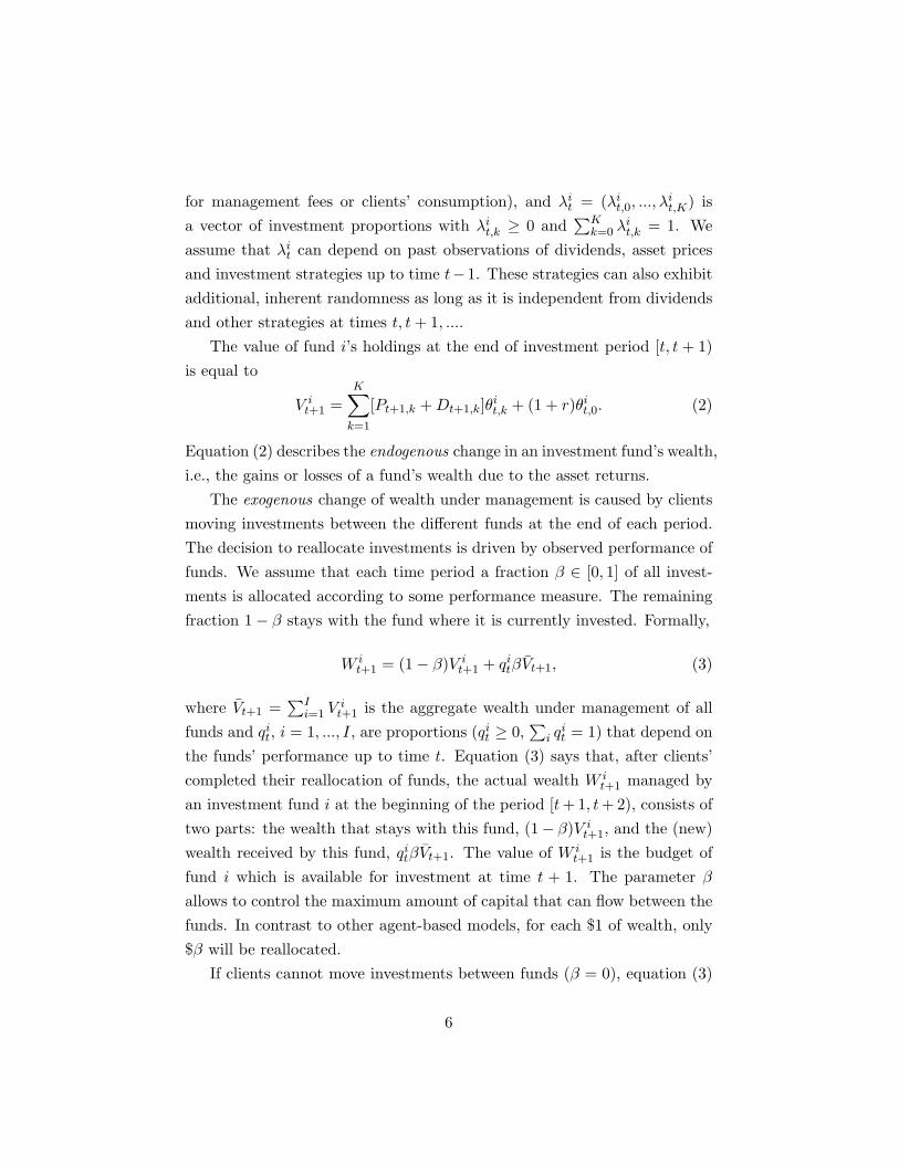
volatility and trading volume. The causes for these observed high pricevolatility and trading volume can be quite different. To illustrate the driversbehind the high price volatility and trading volume, Figure 1 depicts the timeseries of the price of the risky asset and the funds’ wealth under managementwhen γ = 2, and Figure 2 does the same for γ = 8. When the value of γ isrelatively low (γ = 2), itchy-feet clients are less sensitive to the performanceof each fund type leading to a well diversified wealth distribution among thethree fund types. The low level of net flows of wealth which is implied bythe low value of γ serves as a macro level manifestation of the conservatismbias of the itchy-feet clients. The scenario corresponds to that in the bottomrow of Table 3.

Figure 1 illustrates that for low intensities of choice (γ = 2) the wealthmanaged by each of the three funds is almost equal. This can be interpretedas a high degree of differences of opinion in the population of clients which,in turn, entails high price volatility and trading volume.

When the intensity is high (γ = 8) clients’ are prone to herding whichcan be viewed as less differences of opinion. Herding causes fluctuations offunds’ wealth under management and thereby drives booms and crashes.These findings reveal that not only a high degree of differences of opinionbut also herding with a lower degree of differences of opinion can cause highprice volatility and trading volume. This finding points to an alternativeexplanation to the differences-of-opinion literature on explaining the hightrading volume observed in real markets.

Moreover, the differences-of-opinion literature usually ignores the evo-lutionary perspectives of financial markets such as adaptation and marketselection. We have shown that, in a evolutionary context, excess fluctuationsof the price which are caused solely by differences of opinion (in terms ofdifferent investment strategies or prior beliefs, different views in strategy se-lections and different interpretations of the public performance measure) areonly a temporary market phenomenon. These differences of opinion are notsufficient to explain the persistence of high trading volume, whereas addi-tional insights can be obtained by analysing investors’ heuristics and biasesin strategy-switching. Our simulation results show that the high trading

25

(a) Price of risky asset

(b) Proportion of wealth under management: fundamental value fund (red,top), trend-chaser fund (green, middle), noise trader fund (blue, bottom)

Figure 1: Time series of funds’ wealth under management (in proportionsof total wealth) for recency bias (ρ = 0.99), all wealth freely flowing (β = 1)and low intensity of choice (γ = 2).

26

(a) Price of risky asset

(b) Proportion of wealth under management: fundamental value fund (red,top), trend-chaser fund (green, middle), noise trader fund (blue, bottom)

Figure 2: High intensity of choice (γ = 8) in the scenario of Figure 1.

volume is triggered by differences of opinion and amplified by conservatismbias or herding behaviour, while it is investors’ recency bias in performanceevaluation which maintains the persistence of differences of opinion and high

27

trading volume.To further illustrate how the values of the intensity of choice impact the

time series of log-returns of the risky asset, Table 5 collects the summarystatistics for 10 different scenarios with γ ranging from 1 to 10. For compar-ison purpose, the path for the noise fund’s investment proportions and thepath for the dividends are fixed across all the scenarios. For each run, thetime series of log-returns are sampled over 10,000 periods after an initial 1million periods.

γ Mean Max. Min. Std. devp-quantile

Skewness Kurtosisp = 1% p = 99%

1 0.000020 0.3023 -0.2545 0.0683 -0.1675 0.1693 0.0453 3.42402 0.000019 0.2779 -0.2501 0.0636 -0.1561 0.1555 0.0434 3.37403 0.000018 0.2620 -0.2453 0.0600 -0.1480 0.1453 0.0392 3.32214 0.000016 0.2539 -0.2410 0.0573 -0.1389 0.1374 0.0323 3.27175 0.000015 0.2467 -0.2384 0.0554 -0.1349 0.1324 0.0267 3.28226 0.000014 0.4605 -0.2653 0.0545 -0.1331 0.1295 0.0895 4.20577 0.000012 0.6818 -0.3128 0.0557 -0.1388 0.1368 0.3969 8.78778 0.000011 1.1125 -0.3949 0.0594 -0.1459 0.1396 1.4351 30.83579 0.000014 1.2360 -0.4941 0.0630 -0.1665 0.1551 1.7602 36.083110 0.000008 0.9861 -1.2813 0.0643 -0.1718 0.1698 0.1880 40.4167

Table 5: Summary statistics for the time series of log-returns of the riskyasset (excluding dividend) under different values of intensity of choice γ.Clients exhibit a mild recency bias, ρ = 0.99. β = 1.

Table 5 shows that increasing γ decreases the mean of log-returns (whicheventually goes to zero). In contrast, the magnitude of maximum and mini-mum log-returns, standard deviations, the length between 1%-quantile and99%-quantile, and kurtosis exhibit a U-shaped pattern with respect to γ.

The values of the 1%-quantile and the 99%-quantile show that 98% of re-turns are bounded in mid ranges with a maximum interval between -17.18%and 16.98%. These 98% of returns as well as the standard deviation of re-turns are quite stable over the whole range of γ. However, huge booms andcrashes occur for higher values of γ as evidenced by the large maximum andminimum returns. The extremely high kurtosis of returns in these cases im-

28

plies that increasing γ increases the frequency of small returns (and reducesthat of high returns) but at the same time makes large price movementsmore extreme.

The reason for this behaviour is as follows. If the intensity of choice isrelatively low, individual investors are not sensitive to the performance ofeach fund type. The aggregate wealth is well diversified across the threefunds most of the time, which leaves some space for a volatile market sincethe fundamental investment fund does not have a comparative advantage interms of relative wealth. If the intensity of choice is high, investors are sensi-tive to the performance of each fund. From time to time, large price changestrigger large shifts of wealth between the funds, and thereby induce furtherprice changes. These in turn feed back to more changes in funds’ wealthshares. (This is illustrated in the insets in Figure 2 (a) and (b)). Duringthese periods, a highly volatile market with booms and crashes ensues. Onthe other hand, the high intensity of choice also increases the average wealthheld in the fundamental investment fund (see Table 4 and Figure 2). Thisleads to lone periods of time where the market is much less volatile.

Another important question is whether the effect of the intensity ofchoice is proportional to the value of β (the proportion of the freely flowingcapital). To this end, we perform the same exercise as in Table 5 but withβ set to 1% (down from 100%). Table 6 depicts the summary statistics forscenarios with relatively low and high values of γ.

γ Mean Max. Min. Std. devp-quantile

Skewness Kurtosisp = 1% p = 99%

1 0.000021 0.2792 -0.2372 0.0643 -0.1559 0.1563 0.0420 3.34282 0.000021 0.2609 -0.2501 0.0597 -0.1443 0.1456 0.0437 3.35969 0.000019 0.2059 -0.2453 0.0419 -0.1028 0.1034 0.0484 3.490610 0.000019 0.2024 -0.1602 0.0404 -0.0997 0.0991 0.0489 3.5129

Table 6: Summary statistics for the time series of log-returns of the riskyasset (excluding dividend) under different values of intensity of choice γ.Clients exhibit a mild recency bias, ρ = 0.99. β = 0.01.

Comparing the results in Tables 5 and 6 we find the following. When

29

the value of the intensity of choice is low, reducing the value of β by a factorof one-hundred only has a minor impact on the return series. The standarddeviation in both cases γ = 1 and γ = 2 drops only by 0.4%. Changes inother the magnitude of the maximum and minimum returns, 1%-quantileand 99%-quantile, skewness and kurtosis are also very small. In contrast, ifthe intensity of choice is high, reducing the value of β substantially affects thereturn series. Both skewness and kurtosis are much smaller in Table 6 thanin Table 5 for γ = 9 and γ = 10. The values for the 1% and 99% quantiles areboth closer to zero, and the extremely large booms and crashes disappeared.Based on these results, we can conclude that the market is much moresensitive to changes in the intensity of choice when the parameter β is large.

These findings show that in our model the intensity of choice has a pro-nounced impact on the market dynamics when many investors have itchyfeet. But when the cool heads are much more numerous, the intensity ofchoice has very little impact. This observation might be of interest to empiri-cal researchers. For instance, Boswijk et al. [4] use S&P 500 data to estimatethe intensity of choice in an agent-based model. They find the existence oftwo expectation regimes, one fundamentalist and one trend-following. Butthe intensity of choice is not significantly different from zero. The authorsstress that this is a common result in type-switching regression models be-cause large changes in the intensity of choice cause only small variations inthe wealth holdings of the different investment styles. Our model, in con-trast, shows that the intensity of choice does have a strong impact – butonly if enough investors have itchy feet to generate a sufficient amount offreely flowing capital. Moreover, based on the data of mutual fund flows,statistically significant estimates of the intensity of choice parameter arereported by Goldbaum and Mizrach [24].

4 Conclusion

The paper brings together two strands of literature, agent-based modelsof financial markets where investment funds grow exogenously and evolu-tionary finance where all growth is endogenous. By embedding the discrete

30

choice approach into an evolutionary finance framework, the resulting modelallows the coexistence of itchy-feet investors who tend to desert an under-performing portfolio manager quickly and cool-head investors who wouldstick with their portfolio manager even during long periods of poor perfor-mance. The model separates the clients’ decision problem where to investtheir funds and the amount of capital that flows freely within a period intime. If many investors have itchy feet, more capital will be reallocated butif there are many cool heads, client attrition is low and less capital will movein a period.

Numerical analysis of the model shows that a very small amount of freelyflowing capital can have a huge impact on the market dynamics if clientsexhibit recency bias in evaluating fund performance. In particular, evenwith a mild degree of recency bias, the flow of funds is able to create anevolutionary space where the investment strategies of fundamental trading,trend chasing and the noise trading all survive in the long-run. Moreover, incontrast to pure expectations-based type-switching models, the intensity ofclients’ choice is an important factor in driving excess volatility and extremeprice movements if enough investors have itchy feet.

The approach offers several directions for further research. We only lookat the standard one-asset-one-bond model, and we restrict our analysis to3 decision rules. Further we exclude short-selling and long-leveraging. Thistype of constraint is absent in most agent-based models of financial marketswhich, in general, use borrowing as a main driver for excess volatility. Em-pirical issues are not covered in the paper, and it might be interesting to seehow well a calibration can fit stock index dynamics in real markets.

References

[1] R. Amir, I.V. Evstigneev, and K.R. Schenk-Hoppe. Asset market gamesof survival: A synthesis of evolutionary and dynamic games. Annals ofFinance, 9:121–144, 2013.

31

[2] S. Anderson and P. Ahmed. Mutual funds: Fifty years of researchfindings. Springer Science & Business Media, 2005.

[3] M. Anufriev and P. Dindo. Wealth-driven selection in a financial marketwith heterogeneous agents. Journal of Economic Behavior & Organi-zation, 73:327–358, 2010.

[4] H.P. Boswijk, C.H. Hommes, and S. Manzan. Behavioral heterogeneityin stock prices. Journal of Economic Dynamics and Control, 31:1938–1970, 2007.

[5] G. Bottazzi and P. Dindo. Evolution and market behavior with endoge-nous investment rules. Journal of Economic Dynamics and Control,48:121–146, 2014.

[6] W.A. Branch and B. McGough. Replicator dynamics in a cobweb modelwith rationally heterogeneous expectations. Journal of Economic Be-havior & Organization, 65:224–244, 2008.

[7] S. Brianzoni, C. Mammana, and E. Michetti. Updating wealth in anasset pricing model with heterogeneous agents. Discrete Dynamics inNature and Society, Article ID 676317:1–24, 2010.

[8] W.A. Brock and C.H. Hommes. A rational route to randomness. Econo-metrica, 65:1059–1096, 1997.

[9] W.A. Brock and C.H. Hommes. Heterogeneous beliefs and routes tochaos in a simple asset pricing model. Journal of Economic Dynamicsand Control, 22:1235–1274, 1998.

[10] W.A. Brock and C.H. Hommes. Rational animal spirits. In The theoryof markets. Proceedings of the colloquium Theory of Markets and theirfunctioning. Royal Academy of Arts and Sciences, 1999.

[11] B.R. Bruce, editor. Handbook of Behavioral Finance. Edward ElgarPublishing, 2010.

32

[12] C. Chiarella, R. Dieci, and L. Gardini. Speculative behaviour and com-plex asset price dynamics: a global analysis. Journal of EconomicBehavior & Organization, 49:173–197, 2002.

[13] C. Chiarella, R. Dieci, and L. Gardini. Asset price and wealth dynamicsin a financial market with heterogeneous agents. Journal of EconomicDynamics and Control, 30:1755–1786, 2006.

[14] C. Chiarella, R. Dieci, and X.-Z. He. Heterogeneity, market mechanims,and asset price dynamics. In T. Hens and K.R. Schenk-Hoppe, editors,Handbook of Financial Markets: Dynamics and Evolution, pages 277–566. North-Holland, 2009.

[15] C. Chiarella and X.-Z. He. Asset price and wealth dynamics underheterogeneous expectations. Quantitative Finance, 1:509–526, 2001.

[16] G.M. Constantinides, M. Harris, and R.M. Stulz. Handbook of theEconomics of Finance: Asset Pricing. North-Holland, 2013.

[17] J.B. De Long, A. Shleifer, L.H. Summers, and R.J. Waldmann. Noisetrader risk in financial markets. Journal of Political Economy, 98:703–738, 1990.

[18] R. Dieci, I. Foroni, L. Gardini, and X.-Z. He. Market mood, adaptivebeliefs and asset price dynamics. Chaos, Solitons & Fractals, 29:520–534, 2006.

[19] W. Edwards. Conservatism in human information processing. InB. Kleinmuntz, editor, Formal Representation of Human Judgement,pages 17–52. Wiley, 1968.

[20] I.V. Evstigneev, T. Hens, and K.R. Schenk-Hoppe. Evolutionary stablestock markets. Economic Theory, 27:449–468, 2006.

[21] I.V. Evstigneev, T. Hens, and K.R. Schenk-Hoppe. Globally evolution-arily stable portfolio rules. Journal of Economic Theory, 140:197–228,2008.

33

[22] I.V. Evstigneev, T. Hens, and K.R. Schenk-Hoppe. Local stability anal-ysis of a stochastic evolutionary financial market model with a risk-freeasset. Mathematics and Financial Economics, 5:185–202, 2011.

[23] A. Gaunersdorfer and C.H. Hommes. A nonlinear structural modelfor volatility clustering. In G. Teyssiere and A. Kirman, editors, LongMemory in Economics, pages 265–288. Springer, 2007.

[24] D. Goldbaum and B. Mizrach. Estimating the intensity of choice ina dynamic mutual fund allocation decision. Journal of Economic Dy-namics and Control, 32:3866–3876, 2008.

[25] C.H. Hommes. Heterogeneous agent models in economics and finance.In L. Tesfatsion and K.L. Judd, editors, Handbook of ComputationalEconomics, volume 2, pages 1109–1186. Elsevier, 2006.

[26] C.H. Hommes. Behavioral Rationality and Heterogeneous Expectationsin Complex Economic Systems. Cambridge University Press, 2013.

[27] C.H. Hommes, T. Kiseleva, Yu. Kuznetsov, and M. Verbic. Is morememory in evolutionary selection (de)stabilizing? Macroeconomic Dy-namics, 16:335–357, 2012.

[28] C.H. Hommes and F.O.O. Wagener. Complex evolutionary systemsin behavioral finance. In T. Hens and K.R. Schenk-Hoppe, editors,Handbook of Financial Markets: Dynamics and Evolution, pages 217–276. North-Holland, 2009.

[29] B. LeBaron. Empirical regularities from interacting long-and short-memory investors in an agent-based stock market. Evolutionary Com-putation, IEEE Transactions on, 5:442–455, 2001.

[30] B. LeBaron. Evolution and time horizons in an agent-based stock mar-ket. Macroeconomic Dynamics, 5:225–254, 2001.

[31] B. LeBaron. Short-memory traders and their impact on group learningin financial markets. Proceedings of the National Academy of Sciences,99(suppl 3):7201–7206, 2002.

34

[32] B. LeBaron. Agent-based computational finance. In L. Tesfatsion andK.L. Judd, editors, Handbook of Computational Economics, volume 2,pages 1187–1233. Elsevier, 2006.

[33] B. LeBaron. Agent-based financial markets: Matching stylized factswith style. In D. Colander, editor, Post Walrasian Macroeconomics:Beyond the DSGE Model, pages 221–235. Cambridge University Press,2006.

[34] B. LeBaron. Active and passive learning in agent-based financial mar-kets. Eastern Economic Journal, 37:35–43, 2011.

[35] M. Lettau. Explaining the facts with adaptive agents: The case of mu-tual fund flows. Journal of Economic Dynamics and Control, 21:1117–1147, 1997.

[36] M. Levy and H. Levy. The danger of assuming homogeneous expecta-tions. Financial Analysts Journal, 52:65–70, 1996.

[37] M. Levy, H. Levy, and S. Solomon. A microscopic model of the stockmarket: Cycles, booms, and crashes. Economics Letters, 45:103–111,1994.

[38] M. Levy, H. Levy, and S. Solomon. Microscopic simulation of the stockmarket: The effect of microscopic diversity. Journal de Physique I,5:1087–1107, 1995.

[39] M. Levy, H. Levy, and S. Solomon. The Microscopic Simulation of Fi-nancial Markets: From Investor Behavior to Market Phenomena. Aca-demic Press, 2000.

[40] N.G. Mankiw and R. Reis. Sticky information versus sticky prices: Aproposal to replace the new keynesian phillips curve. Quarterly Journalof Economics, pages 1295–1328, 2002.

[41] D. McFadden. Econometric models of probabilistic choice. In C.F.Manski and D. McFadden, editors, Structural Analysis of Discrete Datawith Econometric Applications, pages 198–272. MIT Press, 1981.

35

[42] Y. Murata. Mathematics for Stability and Optimization of EconomicSystems. Elsevier, 1977.

[43] M. Pompian. Behavioral Finance and Wealth Management: How toBuild Optimal Portfolios that Account for Investor Biases. Wiley, 2006.

[44] W. Samuelson and R. Zeckhauser. Status quo bias in decision making.Journal of Risk and Uncertainty, 1:7–59, 1988.

[45] C.A. Sims. Implications of rational inattention. Journal of MonetaryEconomics, 50:665–690, 2003.

[46] T. Wang. Behavioural Biases and Evolutionary Dynamics in an Agent-Based Financial Market. PhD thesis, University of Leeds, 2014.

A Proofs

Proof of Proposition 2.1. Let us first prove an auxiliary result.

Lemma A.1. Let A ∈ RI×K and B ∈ RK×I be non-negative matrices.Suppose

(i)∑I

i=1 Aik < 1 for all k = 1, ...,K; and(ii)

∑Kk=1 Bki ≤ 1 for all i = 1, ..., I.

Then the matrix Id − AB is invertible and the inverse has only strictlypositive elements.

Proof. We show that C = Id−AB has a strict column-dominant diagonal:

I∑j=1,j 6=i

|Cji| < Cii for all i = 1, ..., I. (18)

Then applying Murata [42, Corollary (p. 22) and Theorem 23 (p. 24)] yieldsthe assertion.

As

Cji = 1{i=j} −K∑

k=1

AjkBki

36

and AjkBki ≥ 0, (18) is equivalent to:

I∑j=1

K∑k=1

AjkBki < 1 for all i = 1, ..., I.

Indeed we find that the term on the left-hand side is bounded by

K∑k=1

( I∑j=1

Ajk

)Bki <

K∑k=1

Bki ≤ 1

where we first use assumption (i) and then (ii). �

Proof of Proposition 2.1. Consider the system (5). We apply Lemma A.1to show that the matrix

Id− (1− c)Θt

((1− β)Λt+1 + βΛt+1qt1

)is invertible and that all elements of its inverse are strictly positive. LetA = (1− c)Θt and B = (1− β)Λt+1 + βΛt+1qt1. Since c < 1, one has

I∑i=1

Aik = 1− c < 1.

Further

K∑k=1

Bki = (1− β)K∑

k=1

λik + β

K∑k=1

I∑i=1

λikq

i ≤ 1− β + β = 1.

This gives the result because the non-negative vector

ΘtDt+1 + (1 + r)(1− c)∆λt,0

[(1− β)Vt + βqt−11Vt

]has at least one strictly positive entry. Indeed, by assumption, W i

t = (1 −β)V i

t + βqiVt > 0 and λit,k > 0 for all k ≥ 1. Therefore Θi

t,k > 0. SinceDt+1,k ≥ 0 and

∑Kk=1 Dt+1,k > 0, we finally find

∑Kk=1 Θi

t,kDt+1,k > 0. �

Proof of Proposition 2.2. Recall that the dividend process (Dt) isstationary. Under the assumption of the proposition, the price dynamics (9)

37

can be written asPt+1 = aPt + bDt+1 (19)

with a = a(c, r, λ) and b = b(c, r, λ) defined in (11). The price processhas an autoregressive form with a stationary sequence of innovations bDt+1.Equation (19) has a unique stationary solution if |a| < 1 and the varianceof the innovation is finite. Since a is strictly decreasing in λ, setting λ = 0one finds that a(c, r, 0) ≤ 1 if and only if c ≥ r/(1 + r). Also, a(c, r, 1) = 0,hence, 0 ≤ a < 1. To verify that (10) is a stationary solution to (19), observethat

P ∗t+1 = b

0∑n=−∞

a−nDt+1+n = b−1∑

n=−∞a−nDt+1+n + bDt+1

= ab

0∑n=−∞

a−nDt+n + bDt+1 = aP ∗t + bDt+1.

One has EP ∗t = b/(1− a)ED0 < ∞ and P ∗

t ≥ 0 (as Dt ≥ 0) therefore P ∗t is

finite a.s. Denoting v = V ar(P ∗t ) one obtains the relationship v = a2v+b2σ2

with a unique solution v = b2σ2/(1− a2).Consider any price path Pt with P0 ≥ 0. Then

|Pt − P ∗t | = a|Pt−1 − P ∗

t−1| = · · · = at|P0 − P ∗0 |

which a.s. converges to zero as t →∞. �

Proof of Proposition 2.3. Rearranging equation (15) gives:

qit =

exp(γft)I∑

i=1exp(γft)

=1

1 +∑I

j 6=i exp[γ(f jt − f i

t )]. (20)

38

Inserting (20) into sgn(qit+1 − qi

t) gives:

sgn(qit+1 − qi

t) = sgn

(1

1 +∑I

j 6=i exp[γ(f jt+1 − f i

t+1)]− 1

1 +∑I

j 6=i exp[γ(f jt − f i

t )]

)

= sgn( I∑

j 6=i

exp[γ(f jt − f i

t )]−I∑

j 6=i

exp[γ(f jt+1 − f i

t+1)])

= sgn( I∑

j 6=i

[(f it+1 − f i

t )− (f jt+1 − f j

t )])

= sgn( I∑

j 6=i

(∆it+1 −∆j

t+1))

= sgn(I∆i

t+1 −I∑

j=1

∆jt+1

). (21)

Since dividing I > 0 on the right-hand side of (21) does not change its sign,one has

sgn(qit+1 − qi

t) = sgn

(∆i

t+1 −∑I

j=1 ∆jt+1

I

). (22)

Finally, using ∆t+1 =∑I

j=1 ∆jt+1 in (22) gives:

sgn(qit+1 − qi

t) = sgn(∆it+1 − ∆t+1).

�

B Calibration of dividend distribution

In the numerical analysis the dividends Dt are univariate and i.i.d. withdistribution N (µ, σ2)+ – the normal distribution truncated to non-negativenumbers. We shall show how to choose µ and σ so that the truncateddistribution has a given mean and variance.

Denote by φ+ the density of N (µ, σ2)+. The probability that N (µ, σ2)random variable takes values in the interval R++ is Φ(∞−µ

σ )−Φ(0−µσ ) with

Φ(·) the cumulative distribution function of the standard normal distribu-

39

tion. Therefore, using Bayes theorem the conditional density function isgiven by

φ+(x) =1σφ(x−µ

σ )1− Φ(−µ

σ )=

1σφ(x−µ

σ )Φ(µ

σ ), x ≥ 0,

where φ(x) = e−x2

2√2π

is the probability distribution function of the standardnormal distribution. The expected value is obtained using the moment gen-erating function M(τ) and equals

EDt = M ′(τ)|τ=0 = µ + σφ(h)

Φ(−h)(23)

with h = −µσ . The variance is given by:

V arDt = M ′′(τ)|τ=0 − (M ′(τ)|τ=0)2 = σ2

[1 +

hφ(h)Φ(−h)

−(

φ(h)Φ(−h)

)2]

.

(24)Rewriting the system of equations (23) and (24) gives:

EDt = µ + σφ(h)

Φ(−h), σ2 = V arDt + EDt(EDt − µ). (25)

Inserting σ from the second equation into the first gives a non-linear equa-tion for µ which we solved numerically. When the mean of Dt equals to1 and the standard deviation is 20%, the corresponding parameters forthe truncated normal distribution are µ = 0.9999997026250630 and σ2 =0.0400002973749369.

40