ISYE 2028 Chapter 8 Solutions

Applied Statistics and Probability for Engineers, 5th edition September 22, 2010

8-1

CHAPTER 8

Section 8-1

8-1 a) The confidence level for nxnx /14.2/14.2 σµσ +≤≤− is determined by the value of z0 which is 2.14. From Table III, Φ(2.14) = P(Z<2.14) = 0.9838 and the confidence level is 2(0.9838-0.5) = 96.76%.

b) The confidence level for nxnx /49.2/49.2 σµσ +≤≤− is determined by the by the value of z0 which is 2.14. From Table III, Φ(2.49) = P(Z<2.49) = 0.9936 and the confidence level is is 2(0.9936-0.5) = 98.72%.

c) The confidence level for nxnx /85.1/85.1 σµσ +≤≤− is determined by the by the value of z0 which is 2.14. From Table III, Φ(1.85) = P(Z<1.85) = 0.9678 and the confidence level is 93.56%.

8-2 a) A zα = 2.33 would give result in a 98% two-sided confidence interval. b) A zα = 1.29 would give result in a 80% two-sided confidence interval. c) A zα = 1.15 would give result in a 75% two-sided confidence interval. 8-3 a) A zα = 1.29 would give result in a 90% one-sided confidence interval. b) A zα = 1.65 would give result in a 95% one-sided confidence interval. c) A zα = 2.33 would give result in a 99% one-sided confidence interval. 8-4 a) 95% CI for 96.1,100020,10 , ==== zxn σµ

4.10126.987)10/20(96.11000)10/20(96.11000

//

≤≤

+≤≤−

+≤≤−

µ

µ

σµσ nzxnzx

b) .95% CI for 96.1,100020,25 , ==== zxn σµ

8.10072.992)25/20(96.11000)25/20(96.11000

//

≤≤

+≤≤−

+≤≤−

µ

µ

σµσ nzxnzx

c) 99% CI for 58.2,100020,10 , ==== zxn σµ

3.10167.983)10/20(58.21000)10/20(58.21000

//

≤≤

+≤≤−

+≤≤−

µ

µ

σµσ nzxnzx

d) 99% CI for 58.2,100020,25 , ==== zxn σµ

3.10107.989)25/20(58.21000)25/20(58.21000

//

≤≤

+≤≤−

+≤≤−

µ

µ

σµσ nzxnzx

e) When n is larger, the CI is narrower. The higher the confidence level, the wider the CI.


8-2

8-5 a) Sample mean from the first confidence interval = 38.02 + (61.98-38.02)/2 = 50 Sample mean from the second confidence interval = 39.95 + (60.05-39.95)/2 = 50 b) The 95% CI is (38.02, 61.98) and the 90% CI is (39.95, 60.05). The higher the confidence level, the wider the CI.

8-6 a) Sample mean from the first confidence interval =37.53 + (49.87-37.53)/2 = 43.7

Sample mean from the second confidence interval =35.59 + (51.81-35.59)/2 = 43.7 b) The 99% CI is (35.59, 51.81) and the 95% CI is (37.53, 49.87). The higher the confidence level, the wider the CI.

8-7 a) Find n for the length of the 95% CI to be 40. Za/2 = 1.96

84.320

2.39

202.39

20/)20)(96.1(length 1/2

2

=⎟⎠

⎞⎜⎝

⎛=

=

==

n

n

n

Therefore, n = 4. b) Find n for the length of the 99% CI to be 40. Za/2 = 2.58

66.620

6.51

206.51

20/)20)(58.2(length 1/2

2

=⎟⎠

⎞⎜⎝

⎛=

=

==

n

n

n

Therefore, n = 7.

8-8 Interval (1): 7.32159.3124 ≤≤ µ and Interval (2): 1.32305.3110 ≤≤ µ Interval (1): half-length =90.8/2=45.4 and Interval (2): half-length =119.6/2=59.8 a) 3.31704.459.31241 =+=x

3.31708.595.31102 =+=x The sample means are the same.

b) Interval (1): 7.32159.3124 ≤≤ µ was calculated with 95% Confidence because it has a smaller half-length, and therefore a smaller confidence interval. The 99% confidence level will make the interval larger.

8-9 a) The 99% CI on the mean calcium concentration would be longer.

b) No, that is not the correct interpretation of a confidence interval. The probability that µ is between 0.49 and 0.82 is either 0 or 1. c) Yes, this is the correct interpretation of a confidence interval. The upper and lower limits of the confidence limits are random variables.

8-10 95% Two-sided CI on the breaking strength of yarn: where x = 98, σ = 2 , n=9 and z0.025 = 1.96

3.997.969/)2(96.1989/)2(96.198

// 025.0025.0

≤≤

+≤≤−

+≤≤−

µµ

σµσ nzxnzx

8-11 95% Two-sided CI on the true mean yield: where x = 90.480, σ = 3 , n=5 and z0.025 = 1.96

11.9385.875/)3(96.1480.905/)3(96.1480.90

// 025.0025.0

≤≤

+≤≤−

+≤≤−

µµ

σµσ nzxnzx


8-3

8-12 99% Two-sided CI on the diameter cable harness holes: where x =1.5045 , σ = 0.01 , n=10 and

z0.005 = 2.58

5127.14963.110/)01.0(58.25045.110/)01.0(58.25045.1

// 005.0005.0

≤≤

+≤≤−

+≤≤−

µµ

σµσ nzxnzx

8-13 a) 99% Two-sided CI on the true mean piston ring diameter

For α = 0.01, zα/2 = z0.005 = 2.58 , and x = 74.036, σ = 0.001, n=15

x zn

x zn

−⎛

⎝⎜

⎞

⎠⎟ ≤ ≤ +

⎛

⎝⎜

⎞

⎠⎟0 005 0 005. .

σµ

σ

74 036 258 000115

74 036 258 000115

. . . . . .−

⎛

⎝⎜

⎞

⎠⎟ ≤ ≤ +

⎛

⎝⎜

⎞

⎠⎟µ

74.0353 ≤ µ ≤ 74.0367

b) 99% One-sided CI on the true mean piston ring diameter For α = 0.01, zα = z0.01 =2.33 and x = 74.036, σ = 0.001, n=15

µ

µσ

≤⎟⎟⎠

⎞⎜⎜⎝

⎛−

≤−

15001.033.2036.74

01.0 nzx

74.0354≤ µ The lower bound of the one sided confidence interval is less than the lower bound of the two-sided confidence. This is because the Type I probability of 99% one sided confidence interval (or α = 0.01) in the left tail (or in the lower bound) is greater than Type I probability of 99% two-sided confidence interval (or α/2 = 0.005) in the left tail.

8-14 a) 95% Two-sided CI on the true mean life of a 75-watt light bulb

For α = 0.05, zα/2 = z0.025 = 1.96 , and x = 1014, σ =25 , n=20

⎟⎟⎠

⎞⎜⎜⎝

⎛+≤≤⎟⎟

⎠

⎞⎜⎜⎝

⎛−

nzx

nzx σ

µσ

025.0025.0

10251003202596.11014

202596.11014

≤≤

⎟⎟⎠

⎞⎜⎜⎝

⎛+≤≤⎟⎟

⎠

⎞⎜⎜⎝

⎛−

µ

µ

b) 95% One-sided CI on the true mean piston ring diameter For α = 0.05, zα = z0.05 =1.65 and x = 1014, σ =25 , n=20

µ

µ

µσ

≤

≤⎟⎠

⎞⎜⎝

⎛−

≤−

1005202565.11014

05.0 nzx


8-4

The lower bound of the one sided confidence interval is lower than the lower bound of the two-sided confidence interval even though the level of significance is the same. This is because all of the Type I probability (or α) is in the left tail (or in the lower bound).

8-15 a) 95% two sided CI on the mean compressive strength

zα/2 = z0.025 = 1.96, and x = 3250, σ2 = 1000, n=12

x zn

x zn

−⎛

⎝⎜

⎞

⎠⎟ ≤ ≤ +

⎛

⎝⎜

⎞

⎠⎟0 025 0 025. .

σµ

σ

89.3267 3232.111262.3196.13250

1262.3196.13250

≤≤

⎟⎠

⎞⎜⎝

⎛+≤≤⎟

⎠

⎞⎜⎝

⎛−

µ

µ

b) 99% Two-sided CI on the true mean compressive strength

zα/2 = z0.005 = 2.58

⎟⎠

⎞⎜⎝

⎛+≤≤⎟

⎠

⎞⎜⎝

⎛−

nzx

nzx σ

µσ

005.0005.0

6.3273 3226.41262.3158.23250

1262.3158.23250

≤≤

⎟⎠

⎞⎜⎝

⎛+≤≤⎟

⎠

⎞⎜⎝

⎛−

µ

µ

The 99% CI is wider than the 95% CI 8-16 95% Confident that the error of estimating the true mean life of a 75-watt light bulb is less than 5

hours. For α = 0.05, zα/2 = z0.025 = 1.96 , and σ =25 , E=5

04.965)25(96.1 22

2/ =⎟⎠

⎞⎜⎝

⎛=⎟⎠

⎞⎜⎝

⎛=

Ez

n a σ

Always round up to the next number, therefore n = 97 8-17 Set the width to 6 hours with σ = 25, z0.025 = 1.96 solve for n.

78.2663

49

349

3/)25)(96.1( width1/2

2

=⎟⎠

⎞⎜⎝

⎛=

=

==

n

n

n

Therefore, n = 267. 8-18 99% Confident that the error of estimating the true compressive strength is less than 15 psi

For α = 0.01, zα/2 = z0.005 = 2.58 , and σ =31.62 , E=15

306.2915

)62.31(58.2 222/ ≅=⎟

⎠

⎞⎜⎝

⎛=⎟⎠

⎞⎜⎝

⎛=

Ez

n a σ


8-5

Therefore, n=30 8-19 To decrease the length of the CI by one half, the sample size must be increased by 4 times (22).

lnz 5.0/2/ =σα Now, to decrease by half, divide both sides by 2.

4/)2/(

4/)2/(

2/)2/(2/)/(

22/

2/

2/

lnz

lnz

lnz

=

=

=

σ

σ

σ

α

α

α

Therefore, the sample size must be increased by 22.

8-20 If n is doubled in Eq 8-7: ⎟⎟⎠

⎞⎜⎜⎝

⎛+≤≤⎟⎟

⎠

⎞⎜⎜⎝

⎛−

nzx

nzx σ

µσ

αα 2/2/

⎟⎟⎠

⎞⎜⎜⎝

⎛===

nz

nz

nz

nz σσσσ αααα 2/2/2/2/

414.11

414.1414.12

The interval is reduced by 0.293 29.3% If n is increased by a factor of 4 Eq 8-7:

⎟⎟⎠

⎞⎜⎜⎝

⎛===

nz

nz

nz

nz σσσσ αααα 2/2/2/2/

21

224

The interval is reduced by 0.5 or ½. 8-21 a) 99% two sided CI on the mean temperature

zα/2 = z0.005 = 2.57, and x = 13.77, σ = 0.5, n=11

⎟⎟⎠

⎞⎜⎜⎝

⎛+≤≤⎟⎟

⎠

⎞⎜⎜⎝

⎛−

nzx

nzx σ

µσ

005.0005.0

157.14 13.383115.057.277.13

115.057.277.13

≤≤

⎟⎠

⎞⎜⎝

⎛+≤≤⎟

⎠

⎞⎜⎝

⎛−

µ

µ

b) 95% lower-confidence bound on the mean temperature For α = 0.05, zα = z0.05 =1.65 and x = 13.77, σ = 0.5, n =11

µ

µ

µσ

≤

≤⎟⎟⎠

⎞⎜⎜⎝

⎛−

≤−

521.13115.065.177.13

05.0 nzx

c) 95% confidence that the error of estimating the mean temperature for wheat grown is

less than 2 degrees Celsius. For α = 0.05, zα/2 = z0.025 = 1.96, and σ = 0.5, E = 2

2401.02

)5.0(96.1 222/ =⎟

⎠

⎞⎜⎝

⎛=⎟⎠

⎞⎜⎝

⎛=

Ez

n a σ

Always round up to the next number, therefore n = 1.


8-6

d) Set the width to 1.5 degrees Celsius with σ = 0.5, z0.025 = 1.96 solve for n.

707.175.098.0

75.098.0

75.0/)5.0)(96.1( width1/2

2

=⎟⎠

⎞⎜⎝

⎛=

=

==

n

n

n

Therefore, n = 2. Section 8-2 8-22 131.215,025.0 =t 812.110,05.0 =t 325.120,10.0 =t

787.225,005.0 =t 385.330,001.0 =t

8-23 a) 179.212,025.0 =t b) 064.224,025.0 =t c) 012.313,005.0 =t

d) 073.415,0005.0 =t

8-24 a) 761.114,05.0 =t b) 539.219,01.0 =t c) 467.324,001.0 =t 8-25 a) Mean 1848.25

10848.251

===Nsum

Variance = 5760.2605.1)( 22 === stDev b) 95% confidence interval on mean

605.11848.2510 === sxn 262.29,025.0 =t

333.26037.2410605.1262.21848.25

10605.1262.21848.25

9,025.09,025.0

≤≤

⎟⎠

⎞⎜⎝

⎛+≤≤⎟

⎠

⎞⎜⎝

⎛−

⎟⎠

⎞⎜⎝

⎛+≤≤⎟

⎠

⎞⎜⎝

⎛−

µ

µ

µnstx

nstx

8-26 SE Mean 58.111.6===

NNstDev , therefore N = 15

Mean 0933.501540.751

===Nsum

Variance 3321.3711.6)( 22 === stDev b) 95% confidence interval on mean

11.60933.5015 === sxn 145.214,025.0 =t

477.53709.461511.6145.20933.50

1511.6145.20933.50

14,025.014,025.0

≤≤

⎟⎠

⎞⎜⎝

⎛+≤≤⎟

⎠

⎞⎜⎝

⎛−

⎟⎠

⎞⎜⎝

⎛+≤≤⎟

⎠

⎞⎜⎝

⎛−

µ

µ

µnstx

nstx


8-7

8-27 95% confidence interval on mean tire life 94.36457.139,6016 === sxn 131.215,025.0 =t

07.6208233.581971694.3645131.27.60139

1694.3645131.27.60139

15,025.015,025.0

≤≤

⎟⎟⎠

⎞⎜⎜⎝

⎛+≤≤⎟⎟

⎠

⎞⎜⎜⎝

⎛−

⎟⎟⎠

⎞⎜⎜⎝

⎛+≤≤⎟⎟

⎠

⎞⎜⎜⎝

⎛−

µ

µ

µnstx

nstx

8-28 99% lower confidence bound on mean Izod impact strength 25.025.120 === sxn 539.219,01.0 =t

µ

µ

µ

≤

≤⎟⎟⎠

⎞⎜⎜⎝

⎛−

≤⎟⎟⎠

⎞⎜⎜⎝

⎛−

108.12025.0539.225.1

19,01.0 nstx

8-29 x = 1.10 s = 0.015 n = 25 95% CI on the mean volume of syrup dispensed For α = 0.05 and n = 25, tα/2,n-1 = t0.025,24 = 2.064

106.1 1.09425015.0064.210.1

25015.0064.210.1

24,025.024,025.0

≤≤

⎟⎟⎠

⎞⎜⎜⎝

⎛+≤≤⎟⎟

⎠

⎞⎜⎜⎝

⎛−

⎟⎟⎠

⎞⎜⎜⎝

⎛+≤≤⎟⎟

⎠

⎞⎜⎜⎝

⎛−

µ

µ

µnstx

nstx

8-30 95% confidence interval on mean peak power

163157 === sxn 447.26,025.0 =t

798.329202.3007

315447.2315716447.2315

6,025.06,025.0

≤≤

⎟⎟⎠

⎞⎜⎜⎝

⎛+≤≤⎟⎟

⎠

⎞⎜⎜⎝

⎛−

⎟⎟⎠

⎞⎜⎜⎝

⎛+≤≤⎟⎟

⎠

⎞⎜⎜⎝

⎛−

µ

µ

µnstx

nstx

8-31 99% upper confidence interval on mean SBP 9.93.11814 === sxn 650.213,01.0 =t


8-8

312.125149.9650.23.118

13,005.0

≤

⎟⎠

⎞⎜⎝

⎛+≤

⎟⎟⎠

⎞⎜⎜⎝

⎛+≤

µ

µ

µnstx

8-32 90% CI on the mean frequency of a beam subjected to loads

132.25,n1.53, s231.67, 4,05.1-n/2, ===== ttx α

1.233 230.2553.1132.267.231

553.1132.267.231

4,05.04,05.0

≤≤

⎟⎟⎠

⎞⎜⎜⎝

⎛−≤≤⎟⎟

⎠

⎞⎜⎜⎝

⎛−

⎟⎟⎠

⎞⎜⎜⎝

⎛+≤≤⎟⎟

⎠

⎞⎜⎜⎝

⎛−

µ

µ

µnstx

nstx

By examining the normal probability plot, it appears that the data are normally distributed. There does not appear to be enough evidence to reject the hypothesis that the frequencies are normally distributed.

8-33 The data appear to be normally distributed based on examination of the normal probability plot below.

Therefore, there is evidence to support that the annual rainfall is normally distributed.

236231226

99

95

90

80706050403020

10

5

1

Data

Perc

ent

Normal Probability Plot for frequenciesML Estimates - 95% CI

Mean

StDev

231.67

1.36944

ML Estimates


8-9

Rainfall

Perc

ent

800700600500400300200

99

95

90

80

70

60504030

20

10

5

1

Mean

0.581

485.9StDev 90.30N 20AD 0.288P-Value

Probability Plot of RainfallNormal - 95% CI

95% confidence interval on mean annual rainfall 34.908.48520 === sxn 093.219,025.0 =t

080.528520.4432034.90093.28.485

2034.90093.28.485

19,025.019,025.0

≤≤

⎟⎟⎠

⎞⎜⎜⎝

⎛+≤≤⎟⎟

⎠

⎞⎜⎜⎝

⎛−

⎟⎟⎠

⎞⎜⎜⎝

⎛+≤≤⎟⎟

⎠

⎞⎜⎜⎝

⎛−

µ

µ

µnstx

nstx


Therefore, there is evidence to support that the solar energy is normally distributed.

Solar

Perc

ent

80757065605550

99

95

90

80

70

60504030

20

10

5

1

Mean

0.349


Probability Plot of SolarNormal - 95% CI

95% confidence interval on mean solar energy consumed 225.458.6516 === sxn 131.215,025.0 =t


8-10

831.67329.6316225.4131.258.65

16225.4131.258.65

15,025.015,025.0

≤≤

⎟⎟⎠

⎞⎜⎜⎝

⎛+≤≤⎟⎟

⎠

⎞⎜⎜⎝

⎛−

⎟⎟⎠

⎞⎜⎜⎝

⎛+≤≤⎟⎟

⎠

⎞⎜⎜⎝

⎛−

µ

µ

µnstx

nstx

8-35 99% confidence interval on mean current required

Assume that the data are a random sample from a normal distribution. 7.152.31710 === sxn 250.39,005.0 =t

34.33306.301107.15250.32.317

107.15250.32.317

9,005.09,005.0

≤≤

⎟⎟⎠

⎞⎜⎜⎝

⎛+≤≤⎟⎟

⎠

⎞⎜⎜⎝

⎛−

⎟⎟⎠

⎞⎜⎜⎝

⎛+≤≤⎟⎟

⎠

⎞⎜⎜⎝

⎛−

µ

µ

µnstx

nstx

8-36 a) The data appear to be normally distributed based on examination of the normal probability plot below.

Therefore, there is evidence to support that the level of polyunsaturated fatty acid is normally distributed.

b) 99% CI on the mean level of polyunsaturated fatty acid. For α = 0.01, tα/2,n-1 = t0.005,5 = 4.032

⎟⎟⎠

⎞⎜⎜⎝

⎛+≤≤⎟⎟

⎠

⎞⎜⎜⎝

⎛−

nstx

nstx 5,005.05,005.0 µ

505.17455.166319.0032.498.16

6319.0032.498.16

≤≤

⎟⎟⎠

⎞⎜⎜⎝

⎛+≤≤⎟⎟

⎠

⎞⎜⎜⎝

⎛−

µ

µ

16 17 18

1

5

10

20304050607080

90

95

99

Data

Perc

ent

Normal Probability Plot for 8-25ML Estimates - 95% CI


8-11

The 99% confidence for the mean polyunsaturated fat is (16.455, 17.505). There is high confidence that the true mean is in this interval


b) 95% two-sided confidence interval on mean comprehensive strength

35.62259.912 === sxn 201.211,025.0 =t

5.22823.2237126.35201.29.2259

126.35201.29.2259

11,025.011,025.0

≤≤

⎟⎠

⎞⎜⎝

⎛+≤≤⎟

⎠

⎞⎜⎝

⎛−

⎟⎟⎠

⎞⎜⎜⎝

⎛+≤≤⎟⎟

⎠

⎞⎜⎜⎝

⎛−

µ

µ

µnstx

nstx

c) 95% lower-confidence bound on mean strength

µ

µ

µ

≤

≤⎟⎠

⎞⎜⎝

⎛−

≤⎟⎟⎠

⎞⎜⎜⎝

⎛−

4.2241126.35796.19.2259

11,05.0 nstx

8-38 a) According to the normal probability plot there does not seem to be a severe deviation from normality for

this data. This is due to the fact that the data appears to fall along a straight line.

235022502150

99

95

90

80706050403020

10

5

1

Data

Perc

ent

Normal Probability Plot for StrengthML Estimates - 95% CI

Mean

StDev

2259.92

34.0550

ML Estimates


8-12

b) 95% two-sided confidence interval on mean rod diameter For α = 0.05 and n = 15, tα/2,n-1 = t0.025,14 = 2.145

⎟⎟⎠

⎞⎜⎜⎝

⎛+≤≤⎟⎟

⎠

⎞⎜⎜⎝

⎛−

nstx

nstx 14,025.014,025.0 µ

⎟⎠

⎞⎜⎝

⎛+≤≤⎟

⎠

⎞⎜⎝

⎛−

15025.0145.223.8

15025.0145.223.8 µ

8.216 ≤ µ ≤ 8.244

c) 95% upper confidence bound on mean rod diameter t0.05,14 = 1.761

241.815025.0761.123.8

14,025.0

≤

⎟⎟⎠

⎞⎜⎜⎝

⎛+≤

⎟⎟⎠

⎞⎜⎜⎝

⎛+≤

µ

µ

µnstx


Therefore, there is evidence to support that the speed-up of CNN is normally distributed.

8.308.258.208.15

99

95

90

80706050403020

10

5

1

Data

Perc

ent



8-13

b) 95% confidence interval on mean speed-up

4328.0313.413 === sxn 179.212,025.0 =t

575.4051.4134328.0179.2313.4

134328.0179.2313.4

12,025.012,025.0

≤≤

⎟⎟⎠

⎞⎜⎜⎝

⎛+≤≤⎟⎟

⎠

⎞⎜⎜⎝

⎛−

⎟⎟⎠

⎞⎜⎜⎝

⎛+≤≤⎟⎟

⎠

⎞⎜⎜⎝

⎛−

µ

µ

µnstx

nstx

c) 95% lower confidence bound on mean speed-up

4328.0313.413 === sxn 782.112,05.0 =t

µ

µ

µ

≤

≤⎟⎟⎠

⎞⎜⎜⎝

⎛−

≤⎟⎟⎠

⎞⎜⎜⎝

⎛−

099.4134328.0782.1313.4

12,05.0 nstx

8-40 95% lower bound confidence for the mean wall thickness

given x = 4.05 s = 0.08 n = 25 tα,n-1 = t0.05,24 = 1.711

µ≤⎟⎟⎠

⎞⎜⎜⎝

⎛−

nstx 24,05.0

µ≤⎟⎟⎠

⎞⎜⎜⎝

⎛−

2508.0711.105.4

4.023 ≤ µ There is high confidence that the true mean wall thickness is greater than 4.023 mm.

Speed

Perc

ent

6.05.55.04.54.03.53.0

99

95

90

80

70

60504030

20

10

5

1

Mean

0.745

4.313StDev 0.4328N 13AD 0.233P-Value

Probability Plot of SpeedNormal - 95% CI


8-14

8-41 a) The data appear to be normally distributed. There is not strong evidence that the percentage of enrichment deviates from normality.

b) 99% two-sided confidence interval on mean percentage enrichment For α = 0.01 and n = 12, tα/2,n-1 = t0.005,11 = 3.106, 0.0993s2.9017 ==x

991.2813.212

0.0993106.3902.212

0.0993106.3902.2

11,005.011,005.0

≤≤

⎟⎠

⎞⎜⎝

⎛+≤≤⎟

⎠

⎞⎜⎝

⎛−

⎟⎟⎠

⎞⎜⎜⎝

⎛+≤≤⎟⎟

⎠

⎞⎜⎜⎝

⎛−

µ

µ

µnstx

nstx

3.23.13.02.92.82.72.6

99

95

90

80706050403020

10

5

1

Data

Perc

ent

Normal Probability Plot for Percent EnrichmentML Estimates - 95% CI

Mean

StDev

2.90167

0.0951169

ML Estimates


8-15

Section 8-3 8-42 31.182

10,05.0 =χ 49.27215,025.0 =χ 22.262

12,01.0 =χ

85.10220,95.0 =χ 01.72

18,99.0 =χ 14.5216,995.0 =χ

93.46225,005.0 =χ

8-43 a) 95% upper CI and df = 24 =−

2,1 dfαχ =2

24,95.0χ 13.85

b) 99% lower CI and df = 9 =2,dfαχ =2

9,01.0χ 21.67 c) 90% CI and df = 19

14.30219,05.0

2,2/ == χχα df and 12.102

19,95.02

,2/1 ==− χχ α df 8-44 99% lower confidence bound for σ2 For α = 0.01 and n = 15, =−

21,nαχ =2

14,01.0χ 29.14

2

22

00003075.014.29)008.0(14

σ

σ

≤

≤

8-45 99% lower confidence bound for σ from the previous exercise is

σ

σ

≤

≤

005545.000003075.0 2

One may take the square root of the variance bound to obtain the confidence bound for the standard deviation.

8-46 95% two sided confidence interval for σ

8.410 == sn

02.1929,025.0

21,2/ ==− χχα n and 70.22

9,975.02

1,2/1 ==−− χχ α n

76.830.380.7690.1070.2)8.4(9

02.19)8.4(9

2

22

2

<<

≤≤

≤≤

σ

σ

σ

8-47 95% confidence interval for σ: given n = 51, s = 0.37 First find the confidence interval for σ2 : For α = 0.05 and n = 51, χα/ ,2 1

2n− = χ0 025 50

2. , = 71.42 and χ α1 2 1

2− − =/ ,n χ0 975 50

2. , = 32.36

36.32)37.0(50

42.71)37.0(50 2

22

≤≤σ

0.096 ≤ σ2 ≤ 0.2115 Taking the square root of the endpoints of this interval we obtain, 0.31 < σ < 0.46 8-48 95% confidence interval for σ

09.017 == sn


8-16

85.28216,025.0

21,2/ ==− χχα n and 91.62

16,975.02

1,2/1 ==−− χχ α n

137.0067.00188.00045.091.6)09.0(16

85.28)09.0(16

2

22

2

<<

≤≤

≤≤

σ

σ

σ


Therefore, there is evidence to support that the mean temperature is normally distributed.

95% confidence interval for σ 9463.08 == sn

01.1627,025.0

21,2/ ==− χχα n and 69.12

7,975.02

1,2/1 ==−− χχ α n

926.1626.0709.3392.069.1)9463.0(7

01.16)9463.0(7

2

22

2

<<

≤≤

≤≤

σ

σ

σ

8-50 95% confidence interval for σ

99.1541 == sn

34.59240,025.0

21,2/ ==− χχα n and 43.242

40,975.02

1,2/1 ==−− χχ α n

46.2013.13633.41835.17243.24)99.15(40

34.59)99.15(40

2

22

2

<<

≤≤

≤≤

σ

σ

σ

Mean Temp

Perc

ent

252423222120191817

99

95

90

80

70

60504030

20

10

5

1

Mean

0.367


Probability Plot of Mean TempNormal - 95% CI


8-17

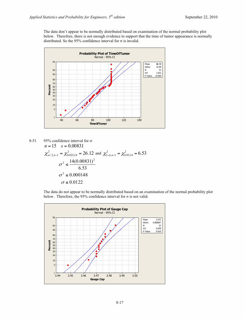
The data don’t appear to be normally distributed based on examination of the normal probability plot below. Therefore, there is not enough evidence to support that the time of tumor appearance is normally distributed. So the 95% confidence interval for σ is invalid.

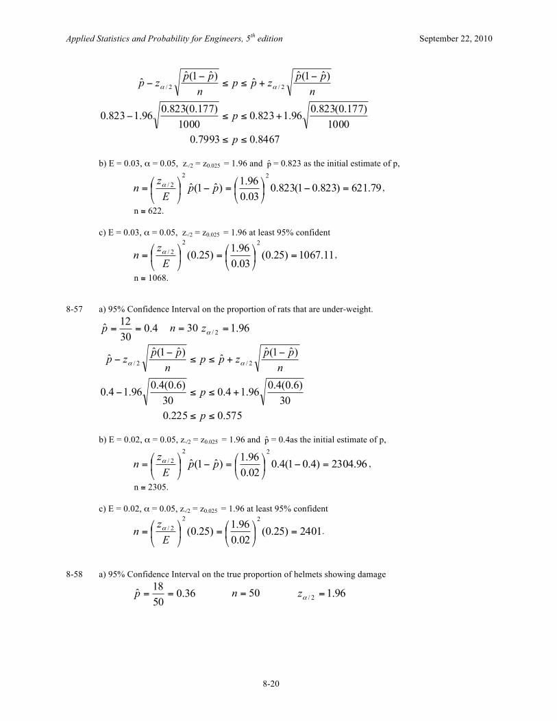
8-51 95% confidence interval for σ

00831.015 == sn

12.26214,025.0

21,2/ ==− χχα n and 53.62

14,95.02

1,1 ==−− χχ α n

0122.0000148.0

53.6)00831.0(14

2

22

≤

≤

≤

σ

σ

σ

The data do not appear to be normally distributed based on an examination of the normal probability plot below. Therefore, the 95% confidence interval for σ is not valid.

TimeOfTumor

Perc

ent

140120100806040

99

95

90

80

70

60504030

20

10

5

1

Mean

<0.005


Probability Plot of TimeOfTumorNormal - 95% CI

Gauge Cap

Perc

ent

3.503.493.483.473.463.453.44

99

95

90

80

70

60504030

20

10

5

1

Mean

0.018

3.472StDev 0.008307N 15AD 0.878P-Value

Probability Plot of Gauge CapNormal - 95% CI


8-18

8-52 a) 99% two-sided confidence interval on σ2 913.110 == sn 59.232

9,005.0 =χ and 73.129,995.0 =χ

038.19396.173.1)913.1(9

59.23)913.1(9

2

22

2

≤≤

≤≤

σ

σ

b) 99% lower confidence bound for σ2

For α = 0.01 and n = 10, =−2

1,nαχ =29,01.0χ 21.67

2

22

5199.167.21)913.1(9

σ

σ

≤

≤

c) 90% lower confidence bound for σ2

For α = 0.1 and n = 10, =−2

1,nαχ =29,1.0χ 14.68

σ

σ

σ

≤

≤

≤

498.12436.268.14)913.1(9

2

22

d) The lower confidence bound of the 99% two-sided interval is less than the one-sided interval. The lower confidence bound for σ2 is in part (c) is greater because the confidence is lower.

Section 8-4 8-53 a) 95% Confidence Interval on the fraction defective produced with this tool.

04333.030013ˆ ==p 300=n 96.12/ =αz

06637.002029.0300

)95667.0(04333.096.104333.0300

)95667.0(04333.096.104333.0

)ˆ1(ˆˆ)ˆ1(ˆˆ 2/2/

≤≤

+≤≤−

−+≤≤

−−

p

p

nppzpp

nppzp αα

b) 95% upper confidence bound 65.105.0 == zzα

06273.0300

)95667.0(04333.0650.104333.0

)ˆ1(ˆˆ 2/

≤

+≤

−+≤

p

p

nppzpp α


8-19

8-54 a) 95% Confidence Interval on the proportion of such tears that will heal.

676.0ˆ =p 37=n 96.12/ =αz

827.05245.037

)324.0(676.096.1676.037

)324.0(676.096.1676.0

)ˆ1(ˆˆ)ˆ1(ˆˆ 2/2/

≤≤

+≤≤−

−+≤≤

−−

p

p

nppzpp

nppzp αα

b) 95% lower confidence bound on the proportion of such tears that will heal.

p

p

pnppzp

≤

≤−

≤−

−

549.037

)33.0(676.064.1676.0

)ˆ1(ˆˆ α

8-55 a) 95% confidence interval for the proportion of college graduates in Ohio that voted for George Bush.

536.0768412ˆ ==p 768=n 96.12/ =αz

571.0501.0768

)464.0(536.096.1536.0768

)464.0(536.096.1536.0

)ˆ1(ˆˆ)ˆ1(ˆˆ 2/2/

≤≤

+≤≤−

−+≤≤

−−

p

p

nppzpp

nppzp αα

b) 95% lower confidence bound on the proportion of college graduates in Ohio that voted for George Bush.

p

p

pnppzp

≤

≤−

≤−

−

506.0768

)464.0(536.064.1536.0

)ˆ1(ˆˆ α

8-56 a) 95% Confidence Interval on the death rate from lung cancer.

823.01000823ˆ ==p 1000=n 96.12/ =αz


8-20

8467.07993.01000

)177.0(823.096.1823.01000

)177.0(823.096.1823.0

)ˆ1(ˆˆ)ˆ1(ˆˆ 2/2/

≤≤

+≤≤−

−+≤≤

−−

p

p

nppzpp

nppzp αα

b) E = 0.03, α = 0.05, zα/2 = z0.025 = 1.96 and p = 0.823 as the initial estimate of p,

79.621)823.01(823.003.096.1)ˆ1(ˆ

222/ =−⎟

⎠

⎞⎜⎝

⎛=−⎟⎠

⎞⎜⎝

⎛= pp

Ez

n α ,

n ≅ 622.

c) E = 0.03, α = 0.05, zα/2 = z0.025 = 1.96 at least 95% confident

11.1067)25.0(03.096.1)25.0(

222/ =⎟

⎠

⎞⎜⎝

⎛=⎟⎠

⎞⎜⎝

⎛=

Ez

n α ,

n ≅ 1068. 8-57 a) 95% Confidence Interval on the proportion of rats that are under-weight.

4.03012ˆ ==p 30=n 96.12/ =αz

575.0225.030

)6.0(4.096.14.030

)6.0(4.096.14.0

)ˆ1(ˆˆ)ˆ1(ˆˆ 2/2/

≤≤

+≤≤−

−+≤≤

−−

p

p

nppzpp

nppzp αα

b) E = 0.02, α = 0.05, zα/2 = z0.025 = 1.96 and p = 0.4as the initial estimate of p,

96.2304)4.01(4.002.096.1)ˆ1(ˆ

222/ =−⎟

⎠

⎞⎜⎝

⎛=−⎟⎠

⎞⎜⎝

⎛= pp

Ez

n α ,

n ≅ 2305.

c) E = 0.02, α = 0.05, zα/2 = z0.025 = 1.96 at least 95% confident

2401)25.0(02.096.1)25.0(

222/ =⎟

⎠

⎞⎜⎝

⎛=⎟⎠

⎞⎜⎝

⎛=

Ez

n α .

8-58 a) 95% Confidence Interval on the true proportion of helmets showing damage

36.05018ˆ ==p 50=n 96.12/ =αz


8-21

493.0227.050

)64.0(36.096.136.050

)64.0(36.096.136.0

)ˆ1(ˆˆ)ˆ1(ˆˆ 2/2/

≤≤

+≤≤−

−+≤≤

−−

p

p

nppzpp

nppzp αα

b) 76.2212)36.01(36.002.096.1)1(

222/ =−⎟

⎠

⎞⎜⎝

⎛=−⎟⎠

⎞⎜⎝

⎛= pp

Ez

n α

2213≅n

c) 2401)5.01(5.002.096.1)1(

222/ =−⎟

⎠

⎞⎜⎝

⎛=−⎟⎠

⎞⎜⎝

⎛= pp

Ez

n α

8-59 The worst case would be for p = 0.5, thus with E = 0.05 and α = 0.01, zα/2 = z0.005 = 2.58 we obtain a

sample size of:

64.665)5.01(5.005.058.2)1(

222/ =−⎟

⎠

⎞⎜⎝

⎛=−⎟

⎠

⎞⎜⎝

⎛= pp

Ezn α , n ≅ 666

8-60 E = 0.017, α = 0.01, zα/2 = z0.005 = 2.58

13.5758)5.01(5.0017.058.2)1(

222/ =−⎟

⎠

⎞⎜⎝

⎛=−⎟

⎠

⎞⎜⎝

⎛= pp

Ezn α , n ≅ 5759

Section 8-6 8-61 95% prediction interval on the life of the next tire given x = 60139.7 s = 3645.94 n = 16 for α=0.05 tα/2,n-1 = t0.025,15 = 2.131

3.681481.521311611)94.3645(131.27.60139

1611)94.3645(131.27.60139

1111

1

1

15,025.0115,025.0

≤≤

++≤≤+−

++≤≤+−

+

+

+

n

n

n

x

x

nstxx

nstx

The prediction interval is considerably wider than the 95% confidence interval (58,197.3 ≤ µ ≤ 62,082.07). This is expected because the prediction interval needs to include the variability in the parameter estimates as well as the variability in a future observation.

8-62 99% prediction interval on the Izod impact data


8-22

25.025.120 === sxn 861.219,005.0 =t

983.1517.02011)25.0(861.225.1

2011)25.0(861.225.1

1111

1

1

19,005.0119,005.0

≤≤

++≤≤+−

++≤≤+−

+

+

+

n

n

n

x

x

nstxx

nstx

The lower bound of the 99% prediction interval is considerably lower than the 99% confidence interval (1.108 ≤ µ ≤ ∞). This is expected because the prediction interval needs to include the variability in the parameter estimates as well as the variability in a future observation.

8-63 95% Prediction Interval on the volume of syrup of the next beverage dispensed

x = 1.10 s = 0.015 n = 25 tα/2,n-1 = t0.025,24 = 2.064

13.1068.12511)015.0(064.210.1

2511)015.0(064.210.1

1111

1

1

24,025.0124,025.0

≤≤

+−≤≤+−

++≤≤+−

+

+

+

n

n

n

x

x

nstxx

nstx

The prediction interval is wider than the confidence interval: 106.1 1.094 ≤≤ µ

8-64 90% prediction interval the value of the natural frequency of the next beam of this type that will be tested.

given x = 231.67, s =1.53 For α = 0.10 and n = 5, tα/2,n-1 = t0.05,4 = 2.132

2.2351.228511)53.1(132.267.231

511)53.1(132.267.231

1111

1

1

4,05.014,05.0

≤≤

+−≤≤+−

++≤≤+−

+

+

+

n

n

n

x

x

nstxx

nstx

The 90% prediction in interval is greater than the 90% CI. 8-65 95% Prediction Interval on the volume of syrup of the next beverage dispensed

34.908.48520 === sxn tα/2,n-1 = t0.025,19 = 2.093

551.679049.2922011)34.90(093.28.485

2011)34.90(093.28.485

1111

1

1

19,025.0119,025.0

≤≤

+−≤≤+−

++≤≤+−

+

+

+

n

n

n

x

x

nstxx

nstx

The 95% prediction interval is wider than the 95% confidence interval. 8-66 99% prediction interval on the polyunsaturated fat


8-23

319.098.166 === sxn 032.45,005.0 =t

37.1859.15611)319.0(032.498.16

611)319.0(032.498.16

1111

1

1

5,005.015,005.0

≤≤

++≤≤+−

++≤≤+−

+

+

+

n

n

n

x

x

nstxx

nstx

The length of the prediction interval is much longer than the width of the confidence interval 505.17455.16 ≤≤ µ . 8-67 Given x = 317.2 s = 15.7 n = 10 for α=0.05 tα/2,n-1 = t0.005,9 = 3.250

7.3707.2631011)7.15(250.32.317

1011)7.15(250.32.317

1111

1

1

9,005.019,005.0

≤≤

+−≤≤+−

++≤≤+−

+

+

+

n

n

n

x

x

nstxx

nstx

The length of the prediction interval is longer. 8-68 95% prediction interval on the next rod diameter tested

025.023.815 === sxn 145.214,025.0 =t

29.817.81511)025.0(145.223.8

1511)025.0(145.223.8

1111

1

1

14,025.0114,025.0

≤≤

+−≤≤+−

++≤≤+−

+

+

+

n

n

n

x

x

nstxx

nstx

95% two-sided confidence interval on mean rod diameter is 8.216 ≤ µ ≤ 8.244 8-69 90% prediction interval on the next specimen of concrete tested

given x = 2260 s = 35.57 n = 12 for α = 0.05 and n = 12, tα/2,n-1 = t0.05,11 = 1.796

5.23265.21931211)57.35(796.12260

1211)57.35(796.12260

1111

1

1

11,05.0111,05.0

≤≤

++≤≤+−

++≤≤+−

+

+

+

n

n

n

x

x

nstxx

nstx

8-70 90% prediction interval on wall thickness on the next bottle tested.


8-24

given x = 4.05 s = 0.08 n = 25 for tα/2,n-1 = t0.05,24 = 1.711

19.491.32511)08.0(711.105.4

2511)08.0(711.105.4

1111

1

1

24,05.0124,05.0

≤≤

+−≤≤+−

++≤≤+−

+

+

+

n

n

n

x

x

nstxx

nstx

8-71 90% prediction interval for enrichment data given x= 2.9 s = 0.099 n = 12 for α = 0.10

and n = 12, tα/2,n-1 = t0.05,11 = 1.796

09.371.21211)099.0(796.19.2

1211)099.0(796.19.2

1111

1

1

12,05.0112,05.0

≤≤

++≤≤+−

++≤≤+−

+

+

+

n

n

n

x

x

nstxx

nstx

The 90% confidence interval is

95.285.2121)099.0(796.19.2

121)099.0(796.19.2

1112,05.012,05.0

≤≤

−≤≤−

+≤≤−

µ

µ

µn

stxn

stx

The prediction interval is wider than the CI on the population mean with the same confidence. The 99% confidence interval is

99.281.2121)099.0(106.39.2

121)099.0(106.39.2

1112,005.012,005.0

≤≤

+≤≤−

+≤≤−

µ

µ

µn

stxn

stx

The prediction interval is even wider than the CI on the population mean with greater confidence.

8-72 To obtain a one sided prediction interval, use tα,n-1 instead of tα/2,n-1 Since we want a 95% one sided prediction interval, tα/2,n-1 = t0.05,24 = 1.711 and x = 4.05 s = 0.08 n = 25

1

1

124,05.0

91.32511)08.0(711.105.4

11

+

+

+

≤

≤+−

≤+−

n

n

n

x

x

xn

stx

The prediction interval bound is much lower than the confidence interval bound of


8-25

4.023 mm 8-73 95% tolerance interval on the life of the tires that has a 95% CL

given x = 60139.7 s = 3645.94 n = 16 we find k=2.903

( ) ( ))86.70723,54.49555(

94.3645903.27.60139,94.3645903.27.60139,

+−

+− ksxksx

95% confidence interval (58,197.3 ≤ µ ≤ 62,082.07) is shorter than the 95%tolerance interval. 8-74 99% tolerance interval on the Izod impact strength PVC pipe that has a 90% CL

given x=1.25, s=0.25 and n=20 we find k=3.368

( ) ( ))092.2,408.0(

25.0368.325.1,25.0368.325.1,

+−

+− ksxksx

The 99% tolerance interval is much wider than the 99% confidence interval on the population mean (1.090 ≤ µ ≤ 1.410).

8-75 95% tolerance interval on the syrup volume that has 90% confidence level

x = 1.10 s = 0.015 n = 25 and k=2.474

( ) ( ))14.1,06.1(

015.0474.210.1,015.0474.210.1,

+−

+− ksxksx

8-76 99% tolerance interval on the polyunsaturated fatty acid in this type of margarine that has a confidence level of 95% x = 16.98 s = 0.319 n=6 and k = 5.775

( ) ( ))82.18,14.15(

319.0775.598.16,319.0775.598.16,

+−

+− ksxksx

The 99% tolerance interval is much wider than the 99% confidence interval on the population mean (16.46 ≤ µ ≤ 17.51).

8-77 95% tolerance interval on the rainfall that has a confidence level of 95%

34.908.48520 === sxn 752.2=k

( ) ( ))416.734,184.237(

34.90752.28.485,34.90752.28.485,

+−

+− ksxksx

The 95% tolerance interval is much wider than the 95% confidence interval on the population mean (08.52852.443 ≤≤ µ ).

8-78 95% tolerance interval on the diameter of the rods in exercise 8-27 that has a 90% confidence level

x = 8.23 s = 0.0.25 n=15 and k=2.713


8-26

( ) ( ))30.8,16.8(

025.0713.223.8,025.0713.223.8,

+−

+− ksxksx

The 95% tolerance interval is wider than the 95% confidence interval on the population mean (8.216 ≤ µ ≤ 8.244).

8-79 99% tolerance interval on the brightness of television tubes that has a 95% CL


( ) ( ))80.386,60.247(

7.15433.42.317,7.15433.42.317,

+−

+− ksxksx

The 99% tolerance interval is much wider than the 95% confidence interval on the population mean

34.33306.301 ≤≤ µ .

8-80 90% tolerance interval on the comprehensive strength of concrete that has a 90% CL given x = 2260 s = 35.57 n = 12 we find k=2.404

( ) ( ))5.2345,5.2174(

57.35404.22260,57.35404.22260,

+−

+− ksxksx

The 90% tolerance interval is much wider than the 95% confidence interval on the population mean

5.22823.2237 ≤≤ µ . 8-81 99% tolerance interval on rod enrichment data that have a 95% CL

given x= 2.9 s = 0.099 n = 12 we find k=4.150

( ) ( ))31.3,49.2(

099.0150.49.2,099.0150.49.2,

+−

+− ksxksx

The 99% tolerance interval is much wider than the 95% CI on the population mean (2.84 ≤ µ ≤ 2.96)

8-82 a) 90% tolerance interval on wall thickness measurements that have a 90% CL


( ) ( ))22.4,88.3(

08.0077.205.4,08.0077.205.4,

+−

+− ksxksx

The lower bound of the 90% tolerance interval is much lower than the lower bound on the 95% confidence interval on the population mean (4.023 ≤ µ ≤ ∞)


8-27

b) 90% lower tolerance bound on bottle wall thickness that has confidence level 90%. given x = 4.05 s = 0.08 n = 25 and k = 1.702

( )91.3

08.0702.105.4 −

− ksx

The lower tolerance bound is of interest if we want to make sure the wall thickness is at least a certain value so that the bottle will not break.


8-28

Supplemental Exercises 8-83 Where ααα =+ 21 . Let 05.0=α

Interval for 025.02/21 === ααα

The confidence level for nxnx /96.1/96.1 σµσ +≤≤− is determined by the by the value of z0

which is 1.96. From Table III, we find Φ(1.96) = P(Z<1.96) = 0.975 and the confidence level is 95%. Interval for 04.0,01.0 21 == αα

The confidence interval is nxnx /75.1/33.2 σµσ +≤≤− , the confidence level is the same because 05.0=α . The symmetric interval does not affect the level of significance; however, it does affect the length. The symmetric interval is shorter in length.

8-84 µ = 50 σ unknown a) n = 16 x = 52 s = 1.5

116/85052

=−

=ot

The P-value for t0 = 1, degrees of freedom = 15, is between 0.1 and 0.25. Thus we would conclude that the results are not very unusual.

b) n = 30

37.130/85052

=−

=ot

The P-value for t0 = 1.37, degrees of freedom = 29, is between 0.05 and 0.1. Thus we conclude that the results are somewhat unusual.

c) n = 100 (with n > 30, the standard normal table can be used for this problem)

5.2100/85052

=−

=oz

The P-value for z0 = 2.5, is 0.00621. Thus we conclude that the results are very unusual. d) For constant values of x and s, increasing only the sample size, we see that the standard error of Xdecreases and consequently a sample mean value of 52 when the true mean is 50 is more unusual for the larger sample sizes.

8-85 5,50 2 == σµ

a) For 16=n find )44.7( 2 ≥sP or )56.2( 2 ≤sP

( ) 10.032.2205.05

)44.7(15)44.7( 2152

215

2 ≤≥≤=⎟⎠

⎞⎜⎝

⎛ ≥=≥ χχ PPSP

Using Minitab )44.7( 2 ≥SP =0.0997

( )≤≤≤=⎟⎠

⎞⎜⎝

⎛ ≤=≤ 68.705.05

)56.2(15)56.2( 215

215

2 χχ PPSP 0.10

Using Minitab )56.2( 2 ≤SP =0.064 b) For 30=n find )44.7( 2 ≥SP or )56.2( 2 ≤SP


8-29

( ) 05.015.43025.05

)44.7(29)44.7( 229

229

2 ≤≥≤=⎟⎠

⎞⎜⎝


Using Minitab )44.7( 2 ≥SP = 0.044

( ) 025.085.1401.05

)56.2(29)56.2( 229

229

2 ≤≤≤=⎟⎠

⎞⎜⎝

⎛ ≤=≤ χχ PPSP

Using Minitab )56.2( 2 ≤SP = 0.014. c) For 71=n )44.7( 2 ≥sP or )56.2( 2 ≤sP

( ) 01.016.104005.05

)44.7(70)44.7( 270

270

2 ≤≥≤=⎟⎠

⎞⎜⎝


Using Minitab )44.7( 2 ≥SP =0.0051

( ) 005.084.355

)56.2(70)56.2( 270

270

2 ≤≤=⎟⎠

⎞⎜⎝

⎛ ≤=≤ χχ PPSP

Using Minitab )56.2( 2 ≤SP < 0.001

d) The probabilities get smaller as n increases. As n increases, the sample variance should approach the population variance; therefore, the likelihood of obtaining a sample variance much larger than the population variance will decrease.

e) The probabilities get smaller as n increases. As n increases, the sample variance should approach the

population variance; therefore, the likelihood of obtaining a sample variance much smaller than the population variance will decrease.

8-86 a) The data appear to follow a normal distribution based on the normal probability plot since the data fall

along a straight line. b) It is important to check for normality of the distribution underlying the sample data since the confidence intervals to be constructed should have the assumption of normality for the results to be reliable (especially since the sample size is less than 30 and the central limit theorem does not apply). c) No, with 95% confidence, we can not infer that the true mean could be 14.05 since this value is not contained within the given 95% confidence interval. d) As with part b, to construct a confidence interval on the variance, the normality assumption must hold for the results to be reliable. e) Yes, it is reasonable to infer that the variance could be 0.35 since the 95% confidence interval on the variance contains this value. f) i) & ii) No, doctors and children would represent two completely different populations not represented by the population of Canadian Olympic hockey players. Because neither doctors nor children were the target of this study or part of the sample taken, the results should not be extended to these groups.

8-87 a) The probability plot shows that the data appear to be normally distributed. Therefore, there is no

evidence conclude that the comprehensive strength data are normally distributed. b) 99% lower confidence bound on the mean 98.42,s25.12, === nx 896.28,01.0 =t


8-30

µ

µ

µ

≤

≤⎟⎟⎠

⎞⎜⎜⎝

⎛−

≤⎟⎟⎠

⎞⎜⎜⎝

⎛−

99.16942.8896.212.25

8,01.0 nstx

The lower bound on the 99% confidence interval shows that the mean comprehensive strength is most likely be greater than 16.99 Megapascals. c) 98% two-sided confidence interval on the mean 98.42,s25.12, === nx 896.28,01.0 =t

25.3399.16942.8896.212.25

942.8896.212.25

8,01.08,01.0

≤≤

⎟⎠

⎞⎜⎝

⎛+≤≤⎟

⎠

⎞⎜⎝

⎛−

⎟⎠

⎞⎜⎝

⎛+≤≤⎟

⎠

⎞⎜⎝

⎛−

µ

µ

µnstx

nstx

The bounds on the 98% two-sided confidence interval shows that the mean comprehensive strength will most likely be greater than 16.99 Megapascals and less than 33.25 Megapascals. The lower bound of the 99% one sided CI is the same as the lower bound of the 98% two-sided CI (this is because of the value of α)

d) 99% one-sided upper bound on the confidence interval on σ2 comprehensive strength

90.70,42.8 2 == ss 65.128,99.0 =χ

74.34365.1)42.8(8

2

22

≤

≤

σ

σ

The upper bound on the 99% confidence interval on the variance shows that the variance of the comprehensive strength is most likely less than 343.74 Megapascals2.

e) 98% two-sided confidence interval on σ2 of comprehensive strength

90.70,42.8 2 == ss 09.2029,01.0 =χ 65.12

8,99.0 =χ

74.34323.2865.1)42.8(8

09.20)42.8(8

2

22

2

≤≤

≤≤

σ

σ

The bounds on the 98% two-sided confidence-interval on the variance shows that the variance of the comprehensive strength is most likely less than 343.74 Megapascals2 and greater than 28.23 Megapascals2. The upper bound of the 99% one-sided CI is the same as the upper bound of the 98% two-sided CI because value of α for the one-sided example is one-half the value for the two-sided example. f) 98% two-sided confidence interval on the mean 96.31,s23, === nx 896.28,01.0 =t


8-31

09.2991.16931.6896.223

931.6896.223

8,01.08,01.0

≤≤

⎟⎟⎠

⎞⎜⎜⎝

⎛+≤≤⎟⎟

⎠

⎞⎜⎜⎝

⎛−

⎟⎟⎠

⎞⎜⎜⎝

⎛+≤≤⎟⎟

⎠

⎞⎜⎜⎝

⎛−

µ

µ

µnstx

nstx

98% two-sided confidence interval on σ2 comprehensive strength

8.39,31.6 2 == ss 09.2029,01.0 =χ 65.12

8,99.0 =χ

97.19285.1565.1)8.39(8

09.20)8.39(8

2

2

≤≤

≤≤

σ

σ

Fixing the mistake decreased the values of the sample mean and the sample standard deviation. Because the sample standard deviation was decreased the widths of the confidence intervals were also decreased. g) The exercise provides s = 8.41 (instead of the sample variance). A 98% two-sided confidence interval on the mean 9,41.8s25, === nx 896.28,01.0 =t

12.3388.16941.8896.225

941.8896.225

8,01.08,01.0

≤≤

⎟⎠

⎞⎜⎝

⎛+≤≤⎟

⎠

⎞⎜⎝

⎛−

⎟⎠

⎞⎜⎝

⎛+≤≤⎟

⎠

⎞⎜⎝

⎛−

µ

µ

µnstx

nstx

98% two-sided confidence interval on σ2 of comprehensive strength

73.70,41.8 2 == ss 09.2029,01.0 =χ 65.12

8,99.0 =χ

94.34216.2865.1)41.8(8

09.20)41.8(8

2

22

2

≤≤

≤≤

σ

σ

Fixing the mistake did not affect the sample mean or the sample standard deviation. They are very close to the original values. The widths of the confidence intervals are also very similar. h) When a mistaken value is near the sample mean, the mistake will not affect the sample mean, standard deviation or confidence intervals greatly. However, when the mistake is not near the sample mean, the value can greatly affect the sample mean, standard deviation and confidence intervals. The farther from the mean, the greater is the effect.

8-88

With σ = 8, the 95% confidence interval on the mean has length of at most 5; the error is then E = 2.5.

a) 34.39645.296.18

5.2

22

2025.0 =⎟

⎠

⎞⎜⎝

⎛=⎟

⎠

⎞⎜⎝

⎛=zn = 40

b) 13.22365.296.16

5.2

22

2025.0 =⎟

⎠

⎞⎜⎝

⎛=⎟

⎠

⎞⎜⎝

⎛=zn = 23


8-32

As the standard deviation decreases, with all other values held constant, the sample size necessary to maintain the acceptable level of confidence and the length of the interval, decreases.

8-89 15.33=x 0.62=s 20=n 564.2=k a) 95% Tolerance Interval of hemoglobin values with 90% confidence

( ) ( ))92.16,74.13(

62.0564.233.15,62.0564.233.15,

+−

+− ksxksx

b) 99% Tolerance Interval of hemoglobin values with 90% confidence 368.3=k

( ) ( ))42.17,24.13(

62.0368.333.15,62.0368.333.15,

+−

+− ksxksx

8-90 95% prediction interval for the next sample of concrete that will be tested.

given x = 25.12 s = 8.42 n = 9 for α = 0.05 and n = 9, tα/2,n-1 = t0.025,8 = 2.306

59.4565.4911)42.8(306.212.25

911)42.8(306.212.25

1111

1

1

8,025.018,025.0

≤≤

++≤≤+−

++≤≤+−

+

+

+

n

n

n

x

x

nstxx

nstx

8-91 a) There is no evidence to reject the assumption that the data are normally distributed.

b) 95% confidence interval on the mean 10,5.7s203.20, === nx 262.29,025.0 =t

228218208198188178

99

95

90

80706050403020

10

5

1

Data

Per

cent

Normal Probability Plot for foam heightML Estimates - 95% CI

Mean

StDev

203.2

7.11056

ML Estimates


8-33

56.20884.1971050.7262.22.203

1050.7262.22.203

9,025.09,025.0

≤≤

⎟⎟⎠

⎞⎜⎜⎝

⎛+≤≤⎟⎟

⎠

⎞⎜⎜⎝

⎛−

⎟⎟⎠

⎞⎜⎜⎝

⎛−≤≤⎟⎟

⎠

⎞⎜⎜⎝

⎛−

µ

µ

µnstx

nstx

c) 95% prediction interval on a future sample

99.22041.1851011)50.7(262.22.203

1011)50.7(262.22.203

1111 9,025.09,025.0

≤≤

++≤≤+−

+−≤≤+−

µ

µ

µn

stxn

stx

d) 95% tolerance interval on foam height with 99% confidence 265.4=k

( ) ( ))19.235,21.171(

5.7265.42.203,5.7265.42.203,

+−

+− ksxksx

e) The 95% CI on the population mean is the narrowest interval. For the CI, 95% of such intervals contain the population mean. For the prediction interval, 95% of such intervals will cover a future data value. This interval is quite a bit wider than the CI on the mean. The tolerance interval is the widest interval of all. For the tolerance interval, 99% of such intervals will include 95% of the true distribution of foam height.

8-92

a) Normal probability plot for the coefficient of restitution. There is no evidence to reject the assumption that the data are normally distributed.

b) 99% CI on the true mean coefficient of restitution x = 0.624, s = 0.013, n = 40 ta/2, n-1 = t0.005, 39 = 2.7079

0.660.650.640.630.620.610.600.59

99

95

90

80706050403020

10

5

1

Data

Perc

ent



8-34

630.0618.040013.07079.2624.0

40013.07079.2624.0

39,005.039,005.0

≤≤

+≤≤−

+≤≤−

µ

µ

µnstx

nstx

c) 99% prediction interval on the coefficient of restitution for the next baseball that will be tested.

660.0588.04011)013.0(7079.2624.0

4011)013.0(7079.2624.0

1111

1

1

39,005.0139,005.0

≤≤

++≤≤+−

++≤≤+−

+

+

+

n

n

n

x

x

nstxx

nstx

d) 99% tolerance interval on the coefficient of restitution with a 95% level of confidence

)666.0,582.0())013.0(213.3624.0),013.0(213.3624.0(

),(+−

+− ksxksx

e) The confidence interval in part (b) is for the population mean and we may interpret this to imply that

99% of such intervals will cover the true population mean. For the prediction interval, 99% of such intervals will cover a future baseball’s coefficient of restitution. For the tolerance interval, 95% of such intervals will cover 99% of the true distribution.

8-93 95% Confidence Interval on the proportion of baseballs with a coefficient of restitution that exceeds 0.635.

2.0408ˆ ==p 40=n 65.1=αz

p

p

pnppzp

≤

≤−

≤−

−

0956.040

)8.0(2.065.12.0

)ˆ1(ˆˆ α

8-94 a) The normal probability shows that the data are mostly follow the straight line, however, there are some

points that deviate from the line near the middle. It is probably safe to assume that the data are normal.


8-35

b) 95% CI on the mean dissolved oxygen concentration

x = 3.265, s = 2.127, n = 20 ta/2, n-1 = t0.025, 19 = 2.093

260.4270.220127.2093.2265.3

20127.2093.2265.3

19,025.019,025.0

≤≤

+≤≤−

+≤≤−

µ

µ

µnstx

nstx

c) 95% prediction interval on the oxygen concentration for the next stream in the system that will be tested..

827.7297.12011)127.2(093.2265.3

2011)127.2(093.2265.3

1111

1

1

19,025.0119,025.0

≤≤−

++≤≤+−

++≤≤+−

+

+

+

n

n

n

x

x

nstxx

nstx

d) 95% tolerance interval on the values of the dissolved oxygen concentration with a 99% level of

confidence

)003.10,473.3())127.2(168.3265.3),127.2(168.3265.3(

),(

−

+−

+− ksxksx


95% of such intervals will cover the true population mean. For the prediction interval, 95% of such intervals will cover a future oxygen concentration. For the tolerance interval, 99% of such intervals will cover 95% of the true distribution

8-95 a) There is no evidence to support that the data are not normally distributed. The data points appear to fall

along the normal probability line.

0 5 10

1

5

10

20304050607080

90

95

99

Data

Per

cent



8-36

b) 99% CI on the mean tar content

x = 1.529, s = 0.0566, n = 30 ta/2, n-1 = t0.005, 29 = 2.756

557.1501.1300566.0756.2529.1

300566.0756.2529.1

29,005.029,005.0

≤≤

+≤≤−

+≤≤−

µ

µ

µnstx

nstx

c) 99% prediction interval on the tar content for the next sample that will be tested..

688.1370.13011)0566.0(756.2529.1

3011)0566.0(756.2529.1

1111

1

1

19,005.0119,005.0

≤≤

++≤≤+−

++≤≤+−

+

+

+

n

n

n

x

x

nstxx

nstx

d) 99% tolerance interval on the values of the tar content with a 95% level of confidence

)719.1,339.1())0566.0(350.3529.1),0566.0(350.3529.1(

),(+−

+− ksxksx


95% of such intervals will cover the true population mean. For the prediction interval, 95% of such intervals will cover a future observed tar content. For the tolerance interval, 99% of such intervals will cover 95% of the true distribution

8-96 a) 95% Confidence Interval on the population proportion

n=1200 x=8 0067.0ˆ =p zα/2=z0.025=1.96

1.4 1.5 1.6 1.7

1

5

10

20304050607080

90

95

99

Data

Per

cent

Normal Probability Plot for tar contentML Estimates - 95% CI

Mean

StDev

1.529

0.0556117

ML Estimates


8-37

0113.00021.01200

)0067.01(0067.096.10067.01200

)0067.01(0067.096.10067.0

)ˆ1(ˆˆ)ˆ1(ˆˆ 2/2/

≤≤

−+≤≤

−−

−+≤≤

−−

p

p

nppzpp

nppzp aa

b) No, there is not sufficient evidence to support the claim that the fraction of defective units produced is one percent or less at α = 0.05. This is because the upper limit of the control limit is greater than 0.01.

8-97 99% Confidence Interval on the population proportion n=1600 x=8 005.0ˆ =p zα/2=z0.005=2.58

009549.00004505.01600

)005.01(005.058.2005.01600

)005.01(005.058.2005.0

)ˆ1(ˆˆ)ˆ1(ˆˆ 2/2/

≤≤

−+≤≤

−−

−+≤≤

−−

p

p

nppzpp

nppzp aa

b) E = 0.008, α = 0.01, zα/2 = z0.005 = 2.58

43.517)005.01(005.0008.058.2)1(

222/ =−⎟

⎠

⎞⎜⎝

⎛=−⎟⎠

⎞⎜⎝

⎛= pp

Ez

n α , n ≅ 518

c) E = 0.008, α = 0.01, zα/2 = z0.005 = 2.58

56.26001)5.01(5.0008.058.2)1(

222/ =−⎟

⎠

⎞⎜⎝

⎛=−⎟⎠

⎞⎜⎝

⎛= pp

Ez

n α , n ≅ 26002

d) A bound on the true population proportion reduces the required sample size by a substantial amount. A sample size of 518 is much more reasonable than a sample size of over 26,000.

8-98 242.0484117ˆ ==p

a) 90% confidence interval; 645.12/ =αz

274.0210.0

)ˆ1(ˆˆ)ˆ1(ˆˆ 2/2/

≤≤

−+≤≤

−−

pnppzpp

nppzp αα

With 90% confidence, the true proportion of new engineering graduates who were planning to continue studying for an advanced degree is between 0.210 and 0.274.

b) 95% confidence interval; zα / .2 196=

280.0204.0

)ˆ1(ˆˆ)ˆ1(ˆˆ 2/2/

≤≤

−+≤≤

−−

pnppzpp

nppzp αα

With 95% confidence, we believe the true proportion of new engineering graduates who were planning to continue studying for an advanced degree lies between 0.204 and 0.280.

c) Comparison of parts (a) and (b):


8-38

The 95% confidence interval is larger than the 90% confidence interval. Higher confidence always yields larger intervals, all other values held constant.

d) Yes, since both intervals contain the value 0.25, thus there in not enough evidence to determine that the true proportion is not actually 0.25.

8-99 a) The data appear to follow a normal distribution based on the normal probability plot since the data fall along a straight line.

b) It is important to check for normality of the distribution underlying the sample data

since the confidence intervals to be constructed should have the assumption of normality for the results to be reliable (especially since the sample size is less than 30 and the central limit theorem does not apply).

c) 95% confidence interval for the mean

33.673.2211 === sxn 228.210,025.0 =t

982.26478.181133.6228.273.22

1133.6228.273.22

10,025.010,025.0

≤≤

⎟⎠

⎞⎜⎝

⎛+≤≤⎟

⎠

⎞⎜⎝

⎛−

⎟⎟⎠

⎞⎜⎜⎝

⎛+≤≤⎟⎟

⎠

⎞⎜⎜⎝

⎛−

µ

µ

µnstx

nstx

d) As with part b, to construct a confidence interval on the variance, the normality

assumption must hold for the results to be reliable.

e) 95% confidence interval for variance 33.611 == sn

48.20210,025.0

21,2/ ==− χχα n and 25.32

10,975.02

1,2/1 ==−− χχ α n

289.123565.1925.3)33.6(10

48.20)33.6(10

2

22

2

≤≤

≤≤

σ

σ


Therefore, there is evidence to support that the energy intake is normally distributed.


8-39

b) 99% upper confidence interval on mean energy (BMR) 5645.0884.510 === sxn 250.39,005.0 =t

464.6304.5105645.0250.3884.5

105645.0250.3884.5

9,005.09,005.0

≤≤

⎟⎟⎠

⎞⎜⎜⎝

⎛+≤≤⎟⎟

⎠

⎞⎜⎜⎝

⎛−

⎟⎟⎠

⎞⎜⎜⎝

⎛+≤≤⎟⎟

⎠

⎞⎜⎜⎝

⎛−

µ

µ

µnstx

nstx

Energy

Perc

ent

87654

99

95

90

80

70

60504030

20

10

5

1

Mean

0.011

5.884StDev 0.5645N 10AD 0.928P-Value

Probability Plot of EnergyNormal - 95% CI


8-40

Mind Expanding Exercises

8-101 a.) αχλχ αα −=<<−

1)2( 2

2,2

2

2,2

1 rr rTP

⎟⎟

⎠

⎞

⎜⎜

⎝

⎛<<=

−

rr TTP

rr

22

2

2,2

2

2,2

1 αα χλ

χ

Then a confidence interval for λ

µ1

= is ⎟⎟

⎠

⎞

⎜⎜

⎝

⎛

−

2

2,2

1

2

2,2

2,2

rr

rr TTαα χχ

b) n = 20 , r = 10 , and the observed value of Tr is 199 + 10(29) = 489.

A 95% confidence interval for λ1

is )98.101,62.28(59.9)489(2,

17.34)489(2

=⎟⎠

⎞⎜⎝

⎛

8-102 dxez

dxez

xx2

212

2

1

211

21

1−−

∫∞−

−=∫∞

=ππ

αα

α

Therefore, )(111 αα zΦ=− .

To minimize L we need to minimize )1()1( 211 αα −Φ+−Φ− subject to ααα =+ 21 . Therefore, we

need to minimize )1()1( 111 ααα +−Φ+−Φ− .

2

21

2

21

2)1(

2)1(

11

1

11

1

αα

α

παα∂α∂

πα∂α∂

−

=+−Φ

−=−Φ

−

−

z

z

e

e

Upon setting the sum of the two derivatives equal to zero, we obtain 2

21

2

21 ααα zz

ee =−

. This is solved by

z zα α α1 1= − . Consequently, ααααα =−= 111 2, and 221ααα == .

8.103 a) n=1/2+(1.9/.1)(9.4877/4), then n=46

b) (10-.5)/(9.4877/4)=(1+p)/(1-p) p=0.6004 between 10.19 and 10.41.

8-104 a)

ni

ni

i

allXPallXPXP

)2/1()~(

)2/1()~(

2/1)~(

=≥

=≤

=≤

µ

µ

µ


8-41

1

21

212

21

21

)()()()(−

⎟⎠

⎞⎜⎝

⎛=⎟⎠

⎞⎜⎝

⎛=⎟⎠

⎞⎜⎝

⎛+⎟⎠

⎞⎜⎝

⎛=

∩−+=∪nnnn

BAPBPAPBAP

n

ii XXPBAP ⎟⎠

⎞⎜⎝

⎛−=<<=∪−211))max(~)(min()(1 µ

b) αµ −=<< 1))max(~)(min( ii XXP The confidence interval is min(Xi), max(Xi)

8-105 We would expect that 950 of the confidence intervals would include the value of µ. This is due to 9the

definition of a confidence interval. Let X bet the number of intervals that contain the true mean (µ). We can use the large sample approximation to determine the probability that P(930 < X < 970).

Let 950.01000950

==p 930.01000930

1 ==p and 970.01000970

2 ==p

The variance is estimated by 1000

)050.0(950.0)1(=

−

npp

9963.0)90.2()90.2(006892.002.0

006892.002.0

1000)050.0(950.0)950.0930.0(

1000)050.0(950.0)950.0970.0()970.0930.0(

=−<−<=⎟⎠

⎞⎜⎝

⎛ −<−⎟

⎠

⎞⎜⎝

⎛ <=

⎟⎟⎟⎟

⎠

⎞

⎜⎜⎜⎜

⎝

⎛

−<−

⎟⎟⎟⎟

⎠

⎞

⎜⎜⎜⎜

⎝

⎛

−<=<<

ZPZPZPZP

ZPZPpP

ISYE 2028 Chapter 8 Solutions

Documents

Transcript of ISYE 2028 Chapter 8 Solutions