ISTANBUL TECHNICAL UNIVERSITY GRADUATE …albertto/dissertations/Mesut_Kirca_PhD_Thesis.pdf ·...

Department of Mechanical Engineering

Mechanical Engineering Programme

ISTANBUL TECHNICAL UNIVERSITY GRADUATE SCHOOL OF SCIENCE

ENGINEERING AND TECHNOLOGY

Ph.D. THESIS

AUGUST 2013

MECHANICS OF NANOMATERIALS

CONSISTED OF RANDOM NETWORKS

Mesut KIRCA

AUGUST 2013

ISTANBUL TECHNICAL UNIVERSITY GRADUATE SCHOOL OF SCIENCE

ENGINEERING AND TECHNOLOGY

MECHANICS OF NANOMATERIALS

CONSISTED OF RANDOM NETWORKS

Ph.D. THESIS

Mesut KIRCA

(503062028)

Department of Mechanical Engineering

Mechanical Engineering Programme

Thesis Advisor: Prof. Dr. Ata MUĞAN

Co-Advisor: Assist. Prof. Albert C. TO

AĞUSTOS 2013

İSTANBUL TEKNİK ÜNİVERSİTESİ FEN BİLİMLERİ ENSTİTÜSÜ

RASTGELE AĞ YAPILI NANO MALZEMELERİN MEKANİĞİ

DOKTORA TEZİ

Mesut KIRCA

(503062028)

Makina Mühendisliği Bölümü

Makine Mühendisliği Programı

Tez Danışmanı: Prof. Dr. Ata MUĞAN

Eş Danışman: Yard. Doç. Dr. Albert C. TO

v

Thesis Advisor : Prof.Dr. Ata MUĞAN ..............................

Istanbul Technical University

Co-Advisor : Assist.Prof. Albert C. TO ..............................

University of Pittsburgh

Jury Members : Prof.Dr. Alaeddin ARPACI .............................


Assoc.Prof. Celaletdin ERGÜN ..............................


Prof.Dr. Uğur GÜVEN ..............................

Yıldız Technical University

Mesut KIRCA, a Ph.D. student of ITU Graduate School of Science, Engineering

and Technology student ID 503062028, successfully defended the dissertation

entitled “MECHANICS OF NANOMATERIALS CONSISTED OF RANDOM

NETWORKS”, which he prepared after fulfilling the requirements specified in the

associated legislations, before the jury whose signatures are below.

Date of Submission : 31 May 2013

Date of Defense : 06 August 2013

Assoc.Prof. Serdar BARIŞ ..............................

Istanbul University

Assist.Prof. Ali GÖKŞENLİ ..............................


vii

To my spouse, Aslıhan and daughter, Defne,

ix

FOREWORD

Firstly, I would like to convey my gratitude to my advisors, Professor Ata Muğan

and Professor Albert C. To, who provided me fundamental advises. They always

supported me strongly in my research studies with availability, patience and

encouragement. I am very grateful for the things that I learnt from them, not only the

scientific matters, but also lots of knowledge which are very helpful in all aspects of

my life. It had been a true privilege to learn from such competent and sincere

supervisors.

Secondly, I would like to offer my great appreciation to my parents and my wife who

have always encouraged and supported me through my many years of academic

endeavors. They are the driving force behind all of my successes. I could not have

accomplished this without them.

August 2013

Mesut KIRCA

xi

TABLE OF CONTENTS

Page

FOREWORD ............................................................................................................. ix TABLE OF CONTENTS .......................................................................................... xi

ABBREVIATIONS ................................................................................................. xiii LIST OF TABLES ................................................................................................... xv LIST OF FIGURES ............................................................................................... xvii

SUMMARY ............................................................................................................. xxi ÖZET ....................................................................................................................... xxv 1. INTRODUCTION .................................................................................................. 1

1.1 Nanomaterials ..................................................................................................... 2 1.1.1 Applications of nanomaterials .................................................................... 3

1.1.2 Classification of nanomaterials ................................................................... 6 1.1.3 Manufacturing of nanomaterials ................................................................. 6

1.2 Introduction to Nanoporous Materials ............................................................... 8

1.2.1 Properties of nanoporous materials ........................................................... 11

1.2.2 Major opportunities in applications of nanoporous materials ................... 11 1.3 Introduction to Carbon Nanotubes ................................................................... 12

1.3.1 Geometry of CNTs .................................................................................... 14

1.3.2 Manufacturing of CNTs ............................................................................ 15 1.3.3 Applications of carbon nanotubes ............................................................. 16

1.4 Purpose of Thesis ............................................................................................. 18

2. OVERVIEW OF MOLECULAR DYNAMICS SIMULATIONS ................... 21 2.1 Introduction ...................................................................................................... 21 2.2 History and Future of MD Simulations ............................................................ 25

2.3 Limitations on MD ........................................................................................... 27

2.4 Time Evolution in MD Simulation ................................................................... 29

2.5 Interatomic Potentials ....................................................................................... 31 2.5.1 Pairwise interactions ................................................................................. 33 2.5.2 Lennard-Jones potential ............................................................................ 33 2.5.3 Embedded atom method ............................................................................ 34 2.5.4 Adaptive intermolecular reactive emprical bond-order potential ............. 35

2.6 Overview of LAMMPS .................................................................................... 36

3. ATOMISTIC MODELLING AND MECHANICS OF NANOPOROUS

MATERIALS ........................................................................................................... 39 3.1 Introduction ...................................................................................................... 39 3.2 Literature Review ............................................................................................. 41

3.2.1 Theoretical and semi-emprical models for macroporous foams ............... 43

3.2.2 Experimental studies on nanoporous foams .............................................. 45

3.2.3 Studies on the Young’s modulus of nanoporous materials ....................... 47 3.2.4 Studies on the yield strength of nanoporous materials ............................. 49 3.2.5 Studies on the Tensile Behavior of Nanoporous Materials ....................... 58

xii

3.3 Atomistic Modeling of Nanoporous Materials ................................................. 61 3.3.1 Random network nature of nanoporous materials..................................... 61 3.3.2 Algorithm for generation of nanoporous models ...................................... 62

3.4 Numerical Experiments .................................................................................... 67

3.5 Results .............................................................................................................. 71 3.6 Summary and Conclusion................................................................................. 76

4. STOCHASTIC MODELING AND MECHANICS OF CARBON

NANOTUBE NETWORKS ..................................................................................... 79 4.1 Purpose ............................................................................................................. 79

4.2 Literature Review ............................................................................................. 79 4.2.1 Elastic modulus of CNTs .......................................................................... 82 4.2.2 Tensile strength of CNTs .......................................................................... 83

4.2.3 Buckling and bending of carbon nanotubes .............................................. 85 4.2.4 Studies on CNT Network Materials .......................................................... 87

4.3 Atomistic Modelling of Heat Welded CNT Networks ..................................... 91 4.3.1 General Concepts ...................................................................................... 91

4.3.2 General Algorithm..................................................................................... 92 4.3.2.1 Line segment representation of CNTs ................................................ 93 4.3.2.2 Target based approach ........................................................................ 94 4.3.2.3 Checking constraints .......................................................................... 96

4.3.2.4 Making decision ................................................................................. 97 4.3.3 Sample Networks and Welding Procedure................................................ 97

4.3.4 Statistical Characterization of Random Networks .................................. 103

4.4 Investigations on the Mechanical Behavior of CNT Networks ...................... 106

4.4.1 Numerical Experiments ........................................................................... 106 4.4.2 Results ..................................................................................................... 109

4.5 Summary and Conclusion............................................................................... 117

5. CONCLUSIONS AND RECOMMENDATIONS ........................................... 121

REFERENCES ....................................................................................................... 127 APPENDICES ........................................................................................................ 139

APPENDIX A ...................................................................................................... 141

CURRICULUM VITAE ........................................................................................ 145

xiii

ABBREVIATIONS

AFM : Atomic Force Microscope

AIREBO : Adaptive Intermolecular Reactive Emprical Bond-Order

CLU : Cubic Lattice Unit

CNT : Carbon Nanotube

CVD : Chemical Vapor Deposition

DIC : Digital Image Correlation

DNA : Deoxyribonucleic Acid

DOE : Department of Energy

EAM : Embedded Atom Method

EBSD : Electron Backscatter Diffraction

EMI : Electromagnetic Interference

FE : Finite Element

HRTEM : High Resolution Transmission Electron Microscope

IUPAC : International Union of Pure and Applied Chemistry

LAMMPS : Large-scale Atomic/Molecular Massively Parallel Simulator

MNP : Metal Nanoparticles

MWNT : Multi-walled Carbon Nanotube

REBO : Reactive Emprical Bond-Order

RNA : Ribonucleic Acid

NP : Nanoporous

SEM : Scanning Electron Microscope

SWNT : Single Walled Carbon Nanotube

TEM : Transmission Electron Microscope

USA : United States of America

xv

LIST OF TABLES

Page

Examples of microporous, mesoporous and macroporous materials. ..... 10 Table 1.1 :

Parameters employed in the random sphere generation algorithm. ....... 69 Table 3.1 :

Experimental studies on the determination of the Young’s modulus of Table 4.1 :

CNTs. ...................................................................................................... 80 Numerical studies on the determination of the Young’s modulus of the Table 4.2 :

CNTs. ...................................................................................................... 81

Summary of quantitative results from tensile loading simulations. ...... 112 Table 4.3 :

Summary of quantitative results from shear loading simulations. ........ 117 Table 4.4 :

xvii

LIST OF FIGURES

Page

Figure 1.1 : From macro-materials to atom. ............................................................... 2 Figure 1.2 : Nanomaterials with different morphologies: (a) Au nanoparticle, (b)

Buckminsterfullerene, (c) FePt nanosphere, (d) Titanium nanoflower,

(e) Silver nanocubes, and (f) SnO2 nanoflower. ..................................... 4 Figure 1.3 : Classification of nanomaterials. .............................................................. 6 Figure 1.4 : Scheme of Top-Down and Bottom-up approaches to the synthesis of

metal nanoparticles (MNP). .................................................................... 7 Figure 1.5 : Specific surface area enhancements: (a) Three blocks having the same

volume initially but different surface areas due to different features, (b)

Surface area increments by splitting a volume. ...................................... 9

Figure 1.6 : Three different types of nanoporous silica materials. (a) A microporous

material: zeolite, (b) A mesoporous material, (c) A macroporous

material. ................................................................................................. 10

Figure 1.7 : Different structural forms of carbon element (a) diamond, (b) graphite,

(c) Lonsdaleite (hexagonal diamoond), (d) Buckminster-Fullerene

(C60), (e) C540, (f) C70, (g) amorphous carbon, (h) Nanotube. .......... 13 Figure 1.8 : (a) Different rolling directions on a graphene sheet causing different

chiralities, (b) General geometric parameters for CNTs. ...................... 15 Figure 1.9 : CNT composites and macrostructures (a) Micrograph showing the cross

section of a carbon fiber laminate with the CNTs dispersed in the epoxy

resin and its application. (b) CNT sheets and yarns used as lightweight

data cables and electromagnetic (EM) shielding material. ................... 17 Figure 2.1 : Examples of nanostructures that can be simulated by MD (a)

Nanowires, (b) Carbon nanotubes, (c) Bio-molecules. ......................... 22

Figure 2.2 : Molecular device design examples (a) Gear chain and (b) Planatary

Gear. ...................................................................................................... 26 Figure 2.3 : MD simulations workflow. .................................................................... 28 Figure 2.4 : (a) Two-body potential parameters, (b) 3-body potential parameters. .. 32 Figure 2.5 : Lennard-Jones potential......................................................................... 34 Figure 3.1 : Sample nanoporous material morphologies: (a) Nanoporous Gold (b)

Nanoporous Platin. ................................................................................ 40 Figure 3.2 : SEM micrographs of 8000-mN indentations on a fractured surface of np

gold: (a) conospherical tip with a tip radius of 0.1 mm, and (b)

Berkovich tip with a curvature of 200 nm. Ductile densification is

observed for both probes. Note that the plastic deformation is confined

to the area under the indenter, and adjacent areas are virtually

undisturbed. ........................................................................................... 51

xviii

Figure 3.3 : Experimental values for foam yield stress for samples of np Au with

relative density ranging from 20% to 42%, normalized by the yield

stress of fully dense Au. The solid line presents the Gibson and Ashby

prediction for a gold foam. .................................................................... 52

Figure 3.4 : The load-displacement curve recorded during in-situ TEM

nanoindentation of a 150 nm np-Au film. It appears that the load drops

(marked by arrows) corresponding to collective collapse of a layer of

pores. ..................................................................................................... 55 Figure 3.5 : True stress-strain curves from 1, 4 and 8 μm diameter nanoporous Au

columns. ................................................................................................ 57 Figure 3.6 : Foam models employed for the mechanical response of carbon foams

(a) Computer Aided Drawing (CAD) model, (b) FEA results of foam

models. .................................................................................................. 62 Figure 3.7 : (a) Representation of a target sphere and its neigbor spheres and (b)

Parameters used for overlapping and non-overlapping ratio calculations.

............................................................................................................... 63

Figure 3.8 : Generation of a CAD foam model by spherical ensemble approach. ... 65 Figure 3.9 : A close view of the CAD model of a sample porous structure. ............ 66 Figure 3.10 : An example of nanoporous models with different porosities (a) 66%

porosity, (b) 70% porosity and (c) with 72% porosity. ......................... 67

Figure 3.11 : Sectioning characterization of nanoporous samples at different

sections. ................................................................................................. 68

Figure 3.12 : (a) Boundary conditions applied on the specimens and (b) Classical

continuum stress-strain relationships where P, A0, L0 are total cross-

sectional force, cross-sectional area and length of the specimen,

respectively. and E are stress, strain and Young’s modulus,

respectively. ........................................................................................... 70 Figure 3.13 : (a) Stress-strain curves for nanoporous aluminum with various

porosities; (b) postpeak tangent modulus as measured from the ultimate

stress point of the corresponding stress-strain curve in (a). .................. 72 Figure 3.14 : Local von Mises stress field during tensile loading of nanoporous -Al

structure with 72% porosity at (a) 1% strain level, (b) 5% strain level,

structure with 78% porosity at (c) 1% strain level and (d) 5% strain

level. ...................................................................................................... 73

Figure 3.15 : Local stress distributions of the structures with 72% and 78%

porosities at 5% strain level. ................................................................. 75 Figure 4.1 : (a) TEM image of a multiwalled carbon nanotube and (b) Schematic of

a multiwalled carbon nanotube. ........................................................... 82 Figure 4.2 : Visualization of tensile loading of a single-walled carbon nanotube by

TEM (a-d) Tensile deformation of a SWNT at high temperature. Kinks

are showed by arrowheads. (e-g) Tensile loading of a SWNT with initial

length of 75nm (e) at room temperature, (f) length after elongation, (g)

length at the failure which is 84nm. ...................................................... 84 Figure 4.3 : Uniaxial compressive loading of a SWNT with 6nm length, 1nm

diameter and armchair chirality of (7,7). ............................................... 86 Figure 4.4 : (a) HREM image of kinking formation of a MWNT with 8nm diameter

and (b) Atomic configuration of a SWNT with a single kink formation

simulated under bending loads. ............................................................. 86 Figure 4.5 : Bending of multi-walled CNTs exhibiting rippling modes of

deformation. .......................................................................................... 87

xix

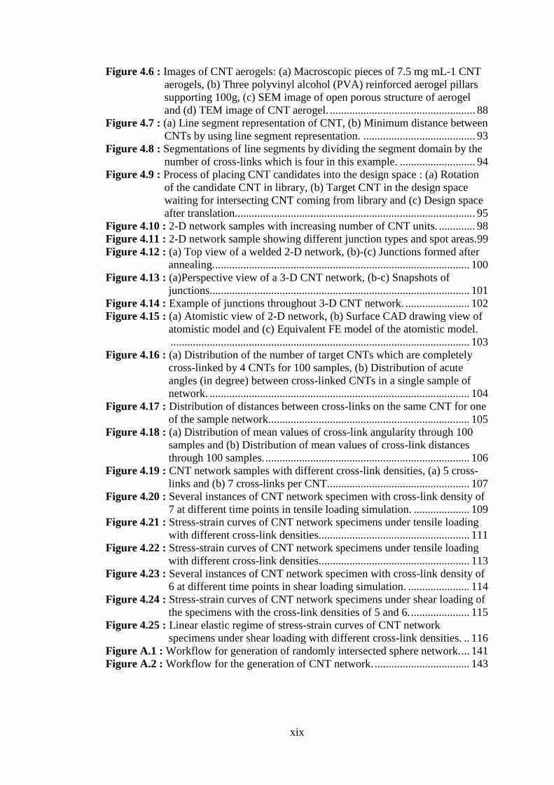
Figure 4.6 : Images of CNT aerogels: (a) Macroscopic pieces of 7.5 mg mL-1 CNT

aerogels, (b) Three polyvinyl alcohol (PVA) reinforced aerogel pillars

supporting 100g, (c) SEM image of open porous structure of aerogel

and (d) TEM image of CNT aerogel. .................................................... 88

Figure 4.7 : (a) Line segment representation of CNT, (b) Minimum distance between

CNTs by using line segment representation. ........................................ 93 Figure 4.8 : Segmentations of line segments by dividing the segment domain by the

number of cross-links which is four in this example. ........................... 94 Figure 4.9 : Process of placing CNT candidates into the design space : (a) Rotation

of the candidate CNT in library, (b) Target CNT in the design space

waiting for intersecting CNT coming from library and (c) Design space

after translation...................................................................................... 95

Figure 4.10 : 2-D network samples with increasing number of CNT units. ............. 98 Figure 4.11 : 2-D network sample showing different junction types and spot areas.99 Figure 4.12 : (a) Top view of a welded 2-D network, (b)-(c) Junctions formed after

annealing. ........................................................................................... 100

Figure 4.13 : (a)Perspective view of a 3-D CNT network, (b-c) Snapshots of

junctions............................................................................................. 101 Figure 4.14 : Example of junctions throughout 3-D CNT network. ....................... 102 Figure 4.15 : (a) Atomistic view of 2-D network, (b) Surface CAD drawing view of

atomistic model and (c) Equivalent FE model of the atomistic model.

........................................................................................................... 103

Figure 4.16 : (a) Distribution of the number of target CNTs which are completely

cross-linked by 4 CNTs for 100 samples, (b) Distribution of acute

angles (in degree) between cross-linked CNTs in a single sample of

network. ............................................................................................. 104

Figure 4.17 : Distribution of distances between cross-links on the same CNT for one

of the sample network. ....................................................................... 105 Figure 4.18 : (a) Distribution of mean values of cross-link angularity through 100

samples and (b) Distribution of mean values of cross-link distances

through 100 samples. ......................................................................... 106

Figure 4.19 : CNT network samples with different cross-link densities, (a) 5 cross-

links and (b) 7 cross-links per CNT................................................... 107 Figure 4.20 : Several instances of CNT network specimen with cross-link density of

7 at different time points in tensile loading simulation. .................... 109 Figure 4.21 : Stress-strain curves of CNT network specimens under tensile loading

with different cross-link densities. ..................................................... 111 Figure 4.22 : Stress-strain curves of CNT network specimens under tensile loading

with different cross-link densities. ..................................................... 113 Figure 4.23 : Several instances of CNT network specimen with cross-link density of

6 at different time points in shear loading simulation. ...................... 114

Figure 4.24 : Stress-strain curves of CNT network specimens under shear loading of

the specimens with the cross-link densities of 5 and 6. ..................... 115 Figure 4.25 : Linear elastic regime of stress-strain curves of CNT network

specimens under shear loading with different cross-link densities. .. 116 Workflow for generation of randomly intersected sphere network. ... 141 Figure A.1 :

Workflow for the generation of CNT network. .................................. 143 Figure A.2 :

xxi

MECHANICS OF NANOMATERIALS CONSISTED OF RANDOM

NETWORKS

SUMMARY

In the field of nanotechnology, nanomaterials with morphological features on the

nanoscale have caught the interest of researchers all around the globe. One class of

these materials which are known as carbon nanotubes (CNTs) is one of the

extraordinary nanomaterials that are promising candidates for thermal, electrical and

structural applications due to their unique properties. Since their discovery by Iijima

(1991), thousands of studies, so far, have been adopted to their exceptional high

strength and unusual electrical and thermal properties, displaying the desirable nature

of their multifunctional capability. In the last years, the usefulness of the CNTs has

been enormously extended by their use as CNT networks through which the CNTs

are self-intersected in two or three dimensional space.

Nanoporous materials with morphological features at the nanoscale have the

potential to be employed as sensors, actuators, insulators, electrodes, energy

absorbents and also for adsorption and separation in recent years. The interest in

studying this class of materials derives from their characteristic high surface-to-

volume ratio. In many of the applications such as actuators, their mechanical

properties are a prerequisite. For example, as actuators, these materials need to

withstand coarsening and sintering. The mechanical strength of nanoporous materials

has been studied through different experimental techniques such as nanoindentation,

beam bending and micro column compression tests.

Due to their random complex structures, randomly structured nanomaterials are

challenging to be modelled and tested numerically. In the proposed thesis, stochastic

methods have been developed to build up numerical models of nanomaterials that are

structured randomly organized nanoscale features such as CNT networked and

nanoporous materials. By using the stochastic methods, sample models for CNT

networks and nanoporous materials have been generated and tested numerically to

show the validity of the stochastic methods and the models generated by them.

Furthermore, generated models have been employed as test specimens within

molecular dynamics simulations to investigate mechanical properties of CNT

network and nanoporous materials.

Both CNT networks and nanoporous materials are examples of random networked

nanomaterials. CNT networks consist of randomly oriented and cross-linked carbon

nanotubes. Nanoporous materials, in a similar way, are built up by randomly oriented

ligaments which are interconnected at junctions. Therefore, both CNT network and

nanoporous materials can be considered as randomly organized materials which are

the subjects of this study.

In the content of this thesis, stochastic models have been developed for random

natured nanomaterials such as CNT network materials and nanoporous materials. For

xxii

this purpose, regarding CNT networked materials, a quasi-random self-intersected

CNT network generation algorithm that enables the control of behavior decisive

parameters, such as CNT length scale, density of junctions and relative angular

position, has been presented and several sample networks with different parameters

mentioned above have been generated. Following the generation of a CNT network

in which the CNT units are so close together that heating to certain temperatures can

yield a covalently bonded network, molecular dynamics (MD) simulations have been

carried out to obtain bonded networks. As a result, parameter-controlled covalently

bonded CNT network models were able to be employed within numerical

simulations to investigate mechanical, thermal and electrical properties of CNT

networks and their co-operating systems (i.e., nanocomposites) for the future studies.

Within stochastic method that has been developed for the CNT network modeling, in

order to save computational time, the CNTs are represented by 3-D line segments

passing through the central points of the CNTs cylindrical geometry.

The atomistic modeling of the nanoporous structures within the proposed thesis study

has been based on an earlier work used to model microcellular carbon foams. The

models have been constructed by initially creating randomly generated spheres that

overlap with each other. After generating enough spheres to cover the desired model

space, the final atomistic model for the nanoporous structure has then been obtained

by deleting from a pristine block the atoms lying within the spheres. In order to

control certain aspects of the topography of the nanoporous structure such as porosity

and ligament size, the following parameters were designed to be adjustable in the

random sphere generation algorithm: (1) range of the size of spheres to be generated,

(2) range of overlapping ratios see below (3) minimum nonoverlapping ratio, and (4)

minimum number of spheres intersecting with any single sphere. Here the

overlapping ratio is defined as the ratio of the distance between the centers of two

overlapping spheres and the sum of their radii. The non-overlapping ratio is defined

as the ratio of the distance between the centers of two non-overlapping spheres and

the sum of their radii.

The general idea behind creating the porous topology is deleting the atoms that fall

inside certain regions within a pristine solid block. These regions are defined by first

interconnecting a “target sphere” with randomly chosen number of “neighbor

spheres”. The neighbor spheres then become the target sphere and each of these

spheres is interconnected with its neighbor spheres. In this way, a network of

interconnected spheres is generated. Atoms that fall inside the regions defined by

these spheres are deleted and what are left behind are the atoms that form ligaments

of the open celled nanoporous structure. One of the restrictions to follow when

generating these spheres is that the neighbor spheres from the same target sphere

cannot overlap each other. The distance between the centers of the two neighbor

spheres can be adjusted by controlling the “non-overlapping ratio”, which is defined

as the ratio between the distance of two non-intersected spheres and sum of the radii

of these two spheres. Another important parameter that influences the overall

porosity of the structure is the “overlapping ratio” between a target sphere and one of

its neighbors. This is defined as the ratio of the distance between the center of the

two spheres and the sum of their radii.

Numerical atomistic models, which have been generated by the stochastics

algorithms, developed for nanoporous and CNT network materials have been

employed in molecular dynamics simulations to test the mechanical behavior of

xxiii

numerical specimens under tensile loading. In a classical MD simulation, the

Newton’s equations of motion are solved to obtain the temporal and spatial

trajectories of atoms, where the force field interactions between the atoms are

described by interatomic potentials derived from quantum mechanical based

calculations. In this way, the state of the atomistic system at any future time can be

predicted from its current state in a deterministic way. The MD method is based on

the assumption that atoms behave like classical particles whose trajectories are

governed by Newton’s equations of motion. With more accurate interatomic

potentials that are obtained by first-principles quantum mechanical (QM)

calculations, engineering properties of nanomaterials obtained through MD

simulations become more faithful and practical. The widely-used MD code

LAMMPS (Large-scale Atomistic/Molecular Massively Parallel Simulator)

developed by the DOE Sandia National Laboratories has been employed to perform

MD simulations on the numerical specimens. The well-tested adaptive

intermolecular reactive empirical bond order (AI-REBO) interatomic potential has

been employed to model the interaction among carbon atoms in CNT networks while

Embedded Atom Method (EAM) potentials have been utilized for the MD

simulations of nanoporous materials.

At the first stage of the proposed study, algortihms of stochastic models for various

nanostructures (i.e., CNT networks and nanoporous materials) have been developed,

which enabled us to generate random natured nanostructures while having control on

the behavior decisive geometric parameters of the corresponding morphology. Then,

the algorithms have been implemented in Matlab environment to generate random

atomistic models of proposed CNT networks and nanoporous materials. Sample

atomistic models have been presented to demonstrate the applicability of developed

algorithms in further computational studies.

At the second stage, generated atomistic models of CNT networks and nanoporous

materials with different morphologic parameters have been employed in MD

simulations to investigate their mechanical behavior subjected tensile loading. In this

regard, atomistic nanoporous specimens with different porosities and different

ligament shapes/sizes have been tested numerically under mechanical loading (i.e.,

tensile loading). By this way, effects of porosity, which is one of the controlled

parameter, on the mechanical behavior of nanoporous materials have been studied

quantitatively. As a result of MD simulations, it has been shown that basic

mechanical properties such as the Young’s modulus, yield and ultimate strength

values of nanoporous materials increases as the porosity decreases. In addition to

that, it has been also demonstrated that softening rate values after the peak stress on

the stress-strain curves for the specimens with higher porosities have been shown to

be slower than the specimens with lower porosities. Detailed evaluation of these

findings considering the deformation mechanisms underlying these differences has

been also provided. Along the same line, random CNT networks generated by the

stochastic method have been used as atomistic models in the MD simulations to

determine the effect of network parameters such as cross link density on the

mechanical behavior under tensile and shear loadings. It has been shown that as the

number of cross links per CNT increases, mechanical properties including elastic

modulus, yield and tensile strength values. The results obtained from numerical tests

perfomed by the MD simulations have been compared with the experimental results

or if-exists numerical results in the literature. Furthermore, basic deformation

xxiv

mechanisms of CNT network materials under tensile and shear loading have been

investigated thoroughly by tracing out the MD simulation snaphots.

xxv

RASTGELE AĞ YAPILI NANO MALZEMELERİN MEKANİĞİ

ÖZET

Hızla gelişen nanoteknoloji alanında nano ölçekteki morfolojik özellikleri ile nano

malzemeler pek çok araştırmacının ilgi odağında olma özelliği kazanmıştır. Nano

malzemelerin bir çeşidi olan karbon nanotüpler ısıl, elektrik ve yapısal özellikleri

itibariyle pek çok potansiyel uygulama alanı bulunan sıra dışı nano malzemelere

verilebilecek en popüler örneklerden biri olarak gösterilebilir. Iijima tarafından 1991

yılındaki keşfedilmesinden sonra karbon nanotüpler üzerinde binlerce akademik

çalışma yapılmış ve olağanüstü yüksek dayanımı, sıra dışı elektriksel ve ısıl

özelliklerinin bir arada olmasından ötürü çok fonksiyonlu kullanılabilme kapasitesi

üzerinde durulmuştur. Özellikle son yıllarda karbon nanotüplerin birbirleriyle 2 veya

3 boyutta kesişmelerinden ibaret olan karbon nanotüp ağ malzemelerin ortaya

çıkmasıyla karbon nanotüplerin makro ölçekteki uygulama alanları daha da

genişletilmiştir.

Nano gözenekli malzemeler de nano ölçekte sahip oldukları yapısal özellikler

sebebiyle nano malzemelerin ilgi toplayan bir başka çeşidi olarak gösterilebilir. Nano

gözenekli malzemeler sensör, eyleyici, yalıtıcı, enerji emici, elektrot ve hatta

soğurucu (adsorption) ve ayırıcı (separation) olarak kullanılma potansiyeli taşıyan

malzemeler olarak son yıllarda ön plana çıkmıştır. Bu malzemeler üzerinde

yoğunlaşan ilginin temelinde nano gözeneklerinden kaynaklanan yüksek

yüzey/hacim oranı yatmaktadır. Bu nedenle bu malzemeler üzerinde yapılacak

çalışmalarda nano gözenek yapısının doğru olarak modellenmesi çok önemlidir.

Bununla beraber, eyleyici olarak kullanılması gibi pek çok uygulamada bu

malzemelerin mekanik özellikleri büyük rol oynamaktadır. Nano gözenekli

malzemelerin mekanik dayanımları nano çentikleme, kiriş eğilmesi, mikro kolon

basma testleri gibi farklı deneysel yöntemlerle incelenmiştir.

Rastgele dağılımlı yapıdaki nano malzemeleri sahip oldukları karmaşık rastgele

yapıları dolayısıyla hem modellenmesi hem de numerik olarak test edilmesi oldukça

zor malzemelerdir. Bu doktora tezinde, rastgele yapısal birimlerden oluşan nano

malzemelerden karbon nanotüp ağ yapılı ve nano gözenekli malzemelerin rastgele

yapılarının sayısal modellenmesi için gerekli yöntemlerin geliştirilmesi

amaçlanmaktadır. Ayrıca, bu yöntemler kullanılarak üretilen sayısal test numuneleri

kullanılarak rastgele modellerin geçerliliğinin gösterilmesi adına moleküler dinamik

(MD) metodu kullanılarak sayısal benzetimler uygulanmıştır. Bununla beraber,

mekanik davranışlarının incelenmesi maksadıyla her iki malzeme tipi için farklı

özelliklerde üretilen test numunelerinin MD yöntemiyle çekme yükü altındaki

davranışı incelenmiştir.

Karbon nanotüp ağ malzemeler, rastgele oryantasyona sahip karbon nanotüplerin

birbirleriyle kesişmelerinden oluşan malzemelerdir. Benzer şekilde, nano gözenekli

malzemeler de rastgele konumlanmış kirişlerin kesiştiği nano kiriş ağı şeklinde

yapılanmıştır. Dolayısıyla hem karbon nanotüp ağ malzemeler hem de nano

xxvi

gözenekli malzemeler rastgele yapılı nano malzemeler sınıfında

değerlendirilebilirler. Rastgele dağılımlı yapısal birimlerden oluşan karmaşık

geometrili bu malzemelerin sayısal olarak modellenebilmeleri için yapılardaki

rastgeleliğin elde edilebilmesi adına özel algoritmaların geliştirilmesine ihtiyaç

duyulmaktadır.

Bu tez kapsamında, yukarıda bahsedilen ihtiyaç doğrultusunda rastgele tabiatlı nano

malzemelerden olan karbon nanotüp ağ yapılı ve nano gözenekli malzemelere ait

rastgele sayısal modellerin oluşturulmasını sağlayan yöntemler geliştirilmiştir. Bu

kapsamda, karbon nanotüp ağ yapılı malzemeler için bazı parametrelerin kontrol

altında tutulabildiği karbon nanotüplerin birbiriyle rastgele olarak kesiştiği bir ağ

yapısının oluşturulabildiği bir algoritma geliştirilmiştir. Bu algoritmada karbon

nanotüp uzunluğu, karbon nanotüp kesişim yoğunluğu ve göreli açısal konum gibi

davranışı etkileyebilecek topolojik parametreler kontrol altına alınmıştır. Farklı

parametreler kullanılarak elde edilen ağ modelleri tez kapsamında sunulmaktadır.

Oluşturulan karbon nanotüp ağ yapılı modeller kullanılarak bir sonraki adımda

moleküler dinamik simülasyonları vasıtasıyla kesişim bölgelerinde lokal olarak

uygulanan ısıtma işlemi neticesinde karbon nanotüpler arasında kovalent bağlar

oluşturulmuş ve bir nevi lokal ısıl kaynağı yapılmıştır. Sonuç olarak kovalent

bağlarla birbirine bağlı karbon nanotüplerden oluşmuş rastgele tabiatlı ağ malzemesi

elde edilmiştir. Bu sayısal modeller söz konusu malzemenin mekanik, ısıl ve elektrik

gibi özelliklerinin incelenmesi adına gelecekteki çalışmalarda kullanılabilecek

niteliktedirler.

Karbon nanotüp ağ yapılı malzemelerin rastgele sayısal modelinin oluşturulmasında

hesaplama zamanını düşürmek amacıyla karbon nanotüpler 3 boyutlu doğru parçaları

olarak modellenmiştir. Söz konusu doğru parçaları silindirik hacimli karbon

nanotüplerin merkez noktalarını birleştiren eksenden geçecek şekilde

oluşturulmuştur.

Diğer yandan, nano gözenekli malzemelerin modellenmesi için geliştirilen yöntemde

ise daha önce mikro gözenekli karbon köpüklerin modellenmesinde kullanılan

yaklaşımdan yola çıkılmıştır. Bu kapsamda ilk adımda birbiriyle belirli oranlarda

rastgele doğrultularda kesişen küresel hacimler topluluğu oluşturulmuştur.

Oluşturulan küresel hacimler topluluğunun büyüklüğü elde edilmek istenen nano

yapının ölçülerinden daha büyük olması gerektiğinin altı çizilmelidir. Yeteri kadar

büyük, birbiriyle kesişen küresel hacimler topluluğu elde edildikten sonra elde

edilmek istenen atomik kafes parametresine sahip malzeme bloğundan küresel

hacimler içerisinde kalan atomların silinmesi suretiyle nano gözenekli yapı elde

edilmiş olur. Boşluk oranı ve kiriş boyutları gibi malzeme davranışını etkileyebilecek

parametreleri kontrol edebilmek adına rastgele kesişimli küresel hacimler

topluluğunun oluşturulması için geliştirilen algoritmada bazı değişkenler kısıt altına

alınarak kontrol edilmiştir. Kısıt altındaki bu değişkenler şöyle sıralanmıştır: (1)

kürelerin çap değişim aralığı, (2) kürelerin kesişme oranı aralığı, (3) aynı küre

üzerinde kesişmeyen küreler arasındaki minimum mesafe oranı, ve (4) aynı küre ile

kesişme halindeki minimum küre sayısı. Bu değişkenlerden kesişim oranının

hesaplanmasında kesişen iki kürenin merkezleri arasındaki mesafe ile yarıçaplarının

toplamı arasındaki oran kullanılır. Benzer şekilde (3) no.lu değişken olan kesişim

yapmayan küreler arasındaki minimum mesafe oranı küreler arasındaki mesafe ile

küre yarıçaplarının toplamı arasında yapılır.

xxvii

Nano gözenekli yapıların sayısal modellenmesindeki genel yaklaşım belirli bir kafes

sistemi parametresine göre oluşturulmuş katı bir hacimsel blok malzemeden, belirli

küresel hacimler içerisinde kalan atomların silinmesi şeklindedir. Bu küresel

hacimler, “hedef” küreler üzerinde birbirleriyle kesişmeden, sadece hedef küre ile

kesişen “komşu” kürelerin yerleştirilmesi ile oluşturulmaktadır. Herhangi bir hedef

küre üzerine yerleştirilebilecek maksimum sayıda komşu küre oluşturulduktan sonra

yeni bir hedef küre seçilerek yeni seçilen hedef kürenin komşu kürelerle donatılması

sağlanmaktadır. Eski komşu küre niteliğindeki kürelerin hedef küre niteliğine

kavuşarak zincirleme etkiyle birbiriyle kesişen küresel hacimler topluluğu

oluşturulmuş olmaktadır. Nihayetinde bu küresel hacimler içerisinde kalan atomların

blok atom topluluğundan çıkartılmasıyla geride nano gözenekli yapının kirişleri ve

bu kirişlerin kesiştikleri alanlar olan eklem bölgeleri ortaya çıkmaktadır. Kürelerin

oluşturulurken kontrol altında tutulan kısıtlardan bir tanesi aynı hedef küre

üzerindeki komşu kürelerin birbiriyle kesişmemesi hususudur. Bunu sağlamak için

aynı hedef küre üzerindeki komşu küreler arasındaki mesafe kontrol altında

tutulmaktadır. Kontrol altındaki bir diğer önemli parametre de boşluk oranını

doğrudan etkileyen, hedef küre ile komşu küreler arasındaki kesişim oranıdır.

Rastgele yapılı nano yapıların sayısal modelleri oluşturulduktan sonra klasik

moleküler dinamik simülasyonlarında kullanılarak numerik modellerin mekanik

davranışının incelenmesi yapılmıştır. Klasik moleküler dinamik simülasyonlarında

Newton’un hareket denklemlerinin çözülmesi suretiyle atomların zaman ve lokasyon

uzay yörüngeleri elde edilir. Bu esnada atomlar arasındaki etkileşimler kuantum

mekaniği hesaplamaları veya tamamen ampirik yöntemler ile oluşturulmuş atomlar

arası potansiyeller vasıtasıyla tanımlanmıştır. Bu şekilde belirli bir andaki atomların

hızları ve konumları kullanılarak bir sonraki zaman adımlarındaki atom koordinat ve

hızlarının elde edilmesiyle deterministik bir sistem çözülmektedir. Moleküler

dinamik metodunda yapılan varsayım atomların, zaman ve mekan yörüngelerinin

Newton’ın hareket denklemleri ile belirlenen klasik parçacıklar gibi davranmasıdır.

Birincil prensipli (first principle) kuantum mekaniği hesaplamalarına dayanarak elde

edilen atomlar arası potansiyellerin kullanıldığı moleküler dinamiği

simülasyonlarıyla sonucu elde edilen nano malzemelerin özelliklerinin güvenilirliği

daha üst seviyededir. Bu çalışmada moleküler dinamik simülasyonlarında LAMMPS

(Large-scale Atomistic/Molecular Massively Parallel Simulator) adı verilen ve USA

DOE Sandia Ulusal Labaratuvar’larında geliştirilmiş açık kodlu ve akademik

çevreler tarafından iyi bilinen bir kod kullanılmıştır. Karbon nanotüp ağ yapıların

simülasyonlarında AIREBO (Adaptive Intermolecular Reactive Empirical Bond

Order) atomlar arası potansiyel olarak kullanılırken nano gözenekli malzemelerin

analizlerinde ise gömülü atom metoduna (Embedded Atom Method, EAM) dayalı

potansiyeller kullanılmıştır.

Bu doktora çalışmasının ilk aşamasında karbon nanotüp ağ yapılı malzemelerin ve

nano gözenekli metal malzemelerin rastgele yapılı sayısal modellerinin oluşturulması

için algoritmalar geliştirildi. Bu algoritmalar vasıtasıyla rastgele tabiatlı adı geçen

malzemelerin davranışlarını etkileyebilecek geometrik parametreler de kontrol

altında tutulmaktadır. Daha sonra bu algoritmalar Matlab programlama dilinde

kodlara dönüştürülerek karbon nanotüp ağ yapılı ve nano gözenekli malzemelerin

sayısal modelleri üretilmiştir.

Çalışmanın ikinci aşamasında ise birinci aşamada geliştirilen algoritmalar ile farklı

morfolojik karakterde üretilen numerik test numuneleri moleküler dinamik

simülasyonlarında kullanılarak mekanik davranışları incelenmiştir. Bu kapsamda,

xxviii

farklı boşluk oranına sahip nano gözenekli test numuneleri kullanılarak MD

yöntemiyle çekme yüklemesi altında test edilerek gerilme-birim şekil değiştirme

eğrileri elde edilmiştir. Boşluk oranı azaldıkça makro gözenekli yapılarda olduğu

gibi nano gözenekli yapıların Young modülü, akma ve çekme mukavemetlerinin

arttığı gözlenmiştir. Bununla beraber, maksimum gerilmenin elde edilmesinden sonra

gözlenen yumuşama (softening) hızının boşluk oranı arttıkça azaldığı ve belli bir

boşluk oranında ise hızlı bir azalmanın olduğu görülmüştür. Yumuşama hızındaki bu

ani değişikliğin nedenleri üzerinde durularak nano gözenekli malzemelerin çekme

yüklemesi altındaki deformasyon mekanizmaları incelenmiştir. Benzer şekilde farklı

kesişim yoğunluklarına sahip karbon nanotüp ağ yapılı numuneler de numerik

mekanik çekme ve kayma testlerine tabii tutulmuştur. Tek bir nanotüp üzerindeki

kesişim yoğunluğunun farklı olduğu sayısal numunelerin çekme ve kayma

benzetimleri sonucunda gerilme-birim şekil değiştirme eğrileri elde edilerek kesişim

yoğunluğu arttıkça mekanik özelliklerde görülen değişiklikler gösterilmiştir. Elde

edilen sonuçlar literatürdeki deneysel veya mevcutsa sayısal sonuçlarla kıyaslanarak

değerlendirilmiştir. Ayrıca, çekme ve kayma yüklemeleri altında karbon nanotüp ağ

yapıların gösterdiği deformasyon mekanizmaları, MD benzetimleri sonucunda

ayrıntılı olarak incelenerek arkasındaki sebepler üzerinde çıkarımlar yapılmıştır.

1

1. INTRODUCTION

Nanoscience and nanotechnology deal with ultra-small things that can be employed

across all scientific disciplines such as chemistry, physics, materials science and

engineering. Nanotechnology that is the ability of controlling the nanostructured

phenomena to achieve a targeted end makes use of nanoscience which is the

understanding of what the nanostructured item behaves.

According to many scientists, the lecture entitled as “There’s plenty of room at the

bottom” given by Nobel Prize awarded physicist Richard Feynman is one of the

milestones that stimulates the ideas behind the development of nanotechnology [1].

Due to unconventional nature of nano-scale world, disciplines that are differentiated

on the continuum scale such as mechanics, materials science and physics are required

to be synthesized on the same core to interpret mysteries of nano-scale world. At this

point, nanoscience is the product of this multi-disciplinary approach to understand

nano-featured processes and characteristics [2-4]. Exciting and highly accelerated

progress that has been established in nanoscience is mainly because of recently

developed capability of controlling and observing the structures at ultra small length

and short time scales together with the highly-developed computational capabilities

that can be utilized to realize numerical experiments.

One billionth of a metre, that is a nanometer (nm), can be approximately visualized

in the minds by several comparisons. For instance, a sheet of paper is about 100,000

nanometers thick while a human hair is roughly 80,000-100,000 nanometers wide.

As more examples, growth rate of human fingernails is at the order of 1nm per

second and a DNA molecule is about 1-2 nm wide. In this regard, Figure 1.1 shows

the relation between macro scale objects and nanoscale world on a scaled axis to

show the transition from macro to nano. Materials at nano scale represent

distinguishing chemical, mechanical, electrical and magnetic behaviors. Even though

nanoscience appears as a new research area, nanomaterials have been used as early

as medieval times. For example, more than thousands year ago gold nano particles

were being added into ceramic porcelains to give red color by Chinese people.

2

Similarly, Roman glass makers were using metal nanoparticles to generate

remarkably nice colors for decoration.

Figure 1.1 : From macro-materials to atom [3].

In many fields of nanotechnology, science of nanomaterials constitutes a basic

building block for the further improvements and innovations. More specifically,

mechanics of nanostructured materials is a very critical area to be understood due to

the fact that many nanosclae phenomena such as folding of proteins that organize a

living cell or the interaction of interfaces between nano-size crystals are controlled or

governed by the mechanics at the nanoscale.

1.1 Nanomaterials

Applications of nanotechnology benefit from the extraordinary properties of

nanomaterials which include at least one property-determining dimension smaller

than 100 nanometer. In the meantime, nanomaterials, or in other words

nanostructured materials consist of structural elements that are in the range of 1 to

100nm, such as nano scale particles, tubes, fibres or rods, can also be thought as the

main products of nanotechnology. One of the basic reasons behind the high interest

in these materials by both academic and industrial environment in recent years is

mostly because of incredible variation of properties observed at continuum and nano

scales [3]. Due to these size-dependent intriguing properties, nanomaterials have

great potential to create impacts in many fields, e.g., aerospace, medicine,

electronics, etc.

3

While some of nanomaterials occur naturally (e.g., volcanic ash and soot from forest

fires), many of nanomaterials can be classified into engineered nanomaterials that are

designed to be manufactured and already being processed to commercial usage.

Nowadays, we realize that many samples of nanomaterials have taken place in the

products of cosmetics, sporting goods, stain-resistant clothing, tires, electronics,

sunscreens and many other stuff that are being used in daily life [5]. Beside these, as

medical applications, nanomaterials are utilized for the purposes of imaging, drug

delivery and diagnosis.

Engineered nanomaterials represent the materials that are designed and manipulated

at nano scale such that they gain novel properties compared with their bulk

counterparts. Two major reasons can be pointed out explaining the different

properties observed at nanomaterials designed at molecular level. One of these is

substantial increase of the surface area due to existence of at least one nanoscale

dimension in the topology of nanomaterials. Increase of surface area results in

greater chemical reactivity of the structures, which in turn affects the mechanical,

electrical and thermal behavior of the material. For example, sensitivity and sensor

selectivity of chemical sensors can be increased by employing nanoparticles and

nanowires due to high surface-to-volume ratio.

The other reason that can be used in the explanation of scale-dependent behavior is

the quantum effect. At the atomic level, quantum effects play much more significant

role in the extraordinary optical, electrical, mechanical and magnetic behaviors of

nanomaterials. Traditionally, basic properties of materials such as the Young’s

modulus are measured by using macroscale or recently microscale test specimens,

which results in no information up-scaled from nano scale. However, properties

determined at macroscale do not predict the behavior of devices that are fabricated

by continuously advancing nanomanufacturing techniques [6].

1.1.1 Applications of nanomaterials

Day by day, appearance of nanomaterials in commercial arena is increasing.

Moreover, the range of available products comprises very large and different fields.

Today, we can find nanomaterials in products of cosmetics, self-cleaning windows,

wrinkle-free or stain-resistant textiles and in many other applications [5].

Nanocomposites and nanocoatings which include nanoscaled particles/fibres to

4

reinforce or change properties of overall bulk material are initiated to be exploited in

variable products such as sports equipment, bicycles, windows and automobiles. For

instance, on glass bottles, novel UV-barrier coatings are used to prevent sunlight

damages on the beverages [3]. Tennis balls with much longer service life can be

achieved by using butyl-rubber/nano-clay composites [3]. As another example,

nanoscale titanium dioxide is employed in cosmetics, sun-protective creams and self-

cleaning windows. Along the same line, nanoscale silica is finding applications as a

filler material in cosmetics and dental operations [4].

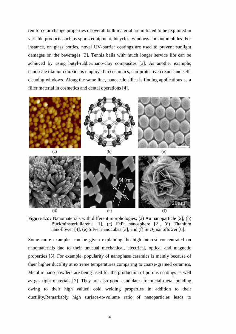
Figure 1.2 : Nanomaterials with different morphologies: (a) Au nanoparticle [2], (b)

Buckminsterfullerene [1], (c) FePt nanosphere [2], (d) Titanium

nanoflower [4], (e) Silver nanocubes [3], and (f) SnO2 nanoflower [6].

Some more examples can be given explaining the high interest concentrated on

nanomaterials due to their unusual mechanical, electrical, optical and magnetic

properties [5]. For example, popularity of nanophase ceramics is mainly because of

their higher ductility at extreme temperatures comparing to coarse-grained ceramics.

Metallic nano powders are being used for the production of porous coatings as well

as gas tight materials [7]. They are also good candidates for metal-metal bonding

owing to their high valued cold welding properties in addition to their

ductility.Remarkably high surface-to-volume ratio of nanoparticles leads to

5

extraordinary improvements of chemical catalysis. The range of potential

applications of nanoparticles in catalysis is very broad to be from fuel cell

applications to catalytic converters and photocatalytic devices [4].

Scientific interest on nanomaterials has begun in the 19th

century despite the fact that

nanomaterials already exist in the nature. Unquestionably, the most important

stimulating factor leading the scientific research on nanomaterials is the development

of high capability of microscopic devices that enable us to observe the nanoscale

world [6]. In 1857, Michael Faraday’s report on the colloidal gold particles can be

shown as one of the first studies on nanomaterials [7]. On the other hand,

investigations on the nanostructured catalysts have been in progress for

approximately over 70 years. In USA and Germany, as a substitution of ultrafine

carbon black for rubber reinforcements, fume silica nano particles were being

manufactured in the beginnings of 1940’s [8]. Extending the examples of

applications of nanomaterials, nanostructured amorphous silica particles have also

been used in many daily life products such as non-diary coffee creamer to

automobile tires and catalyst supports [3]. In the 1960s and 1970s, magnetic

recording tapes were developed to be produced by using metallic nanopowders.

Granqvist and Buhrman published a new technique which is popular now, called the

inert-gas evaporation technique to produce nanocrystals in 1976 [4]. Lately, the

mystery of beautiful tone of Maya blue paint and its resistance to acidic environment

has been explained by its hybrid nanostructure consisting of amorphous silicate

substrate with inclusions of metal (i.e., Mg) nanoparticles [5].

By non-stop progress being achieved in nanotechnology, the number of

nanostructured functional materials which permit altering of mechanical, electrical,

magnetic, optical and electronic functions. Nanophased or cluster-assembled bulk

materials are good examples of this kind of progress. Initially, discrete nano

clusters/particles are manufactured at the first step and then these small

particles/clusters are embedded into liquid or solid matrix materials [6]. As an

example, nanophased silicon that is completely different from conventional silicon in

physical and electrical properties can be employed in macroscopic semiconductor

processes. In another example, conventional glass turns into a high performance

optical medium presenting potential optical computational capability after being

doped with quantized semiconductor colloids [9].

6

1.1.2 Classification of nanomaterials

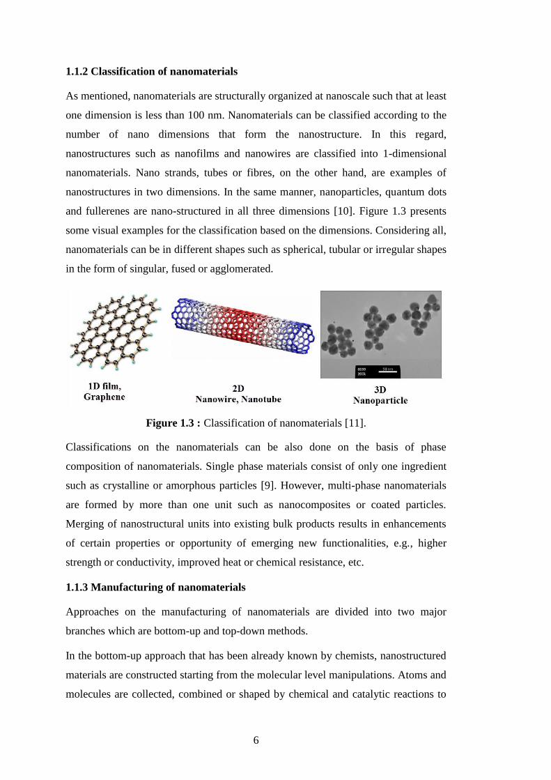
As mentioned, nanomaterials are structurally organized at nanoscale such that at least

one dimension is less than 100 nm. Nanomaterials can be classified according to the

number of nano dimensions that form the nanostructure. In this regard,

nanostructures such as nanofilms and nanowires are classified into 1-dimensional

nanomaterials. Nano strands, tubes or fibres, on the other hand, are examples of

nanostructures in two dimensions. In the same manner, nanoparticles, quantum dots

and fullerenes are nano-structured in all three dimensions [10]. Figure 1.3 presents

some visual examples for the classification based on the dimensions. Considering all,

nanomaterials can be in different shapes such as spherical, tubular or irregular shapes

in the form of singular, fused or agglomerated.

Figure 1.3 : Classification of nanomaterials [11].

Classifications on the nanomaterials can be also done on the basis of phase

composition of nanomaterials. Single phase materials consist of only one ingredient

such as crystalline or amorphous particles [9]. However, multi-phase nanomaterials

are formed by more than one unit such as nanocomposites or coated particles.

Merging of nanostructural units into existing bulk products results in enhancements

of certain properties or opportunity of emerging new functionalities, e.g., higher

strength or conductivity, improved heat or chemical resistance, etc.

1.1.3 Manufacturing of nanomaterials

Approaches on the manufacturing of nanomaterials are divided into two major

branches which are bottom-up and top-down methods.

In the bottom-up approach that has been already known by chemists, nanostructured

materials are constructed starting from the molecular level manipulations. Atoms and

molecules are collected, combined or shaped by chemical and catalytic reactions to

7

form desired nanostructural units [12]. By employing AFM (Atomic Force

Microscope) and using liquid phase techniques based on inverse micelles, bottom-up

approach is being utilized by several nano scale manufacturing techniques such as

chemical vapor deposition (CVD), laser pyrolysis and molecular self-assembly [10].

In this approach, atomic scale structural units, i.e., atoms, molecules or clusters,

arrange themselves into more complex structural units similar to the growth of a

crystal.

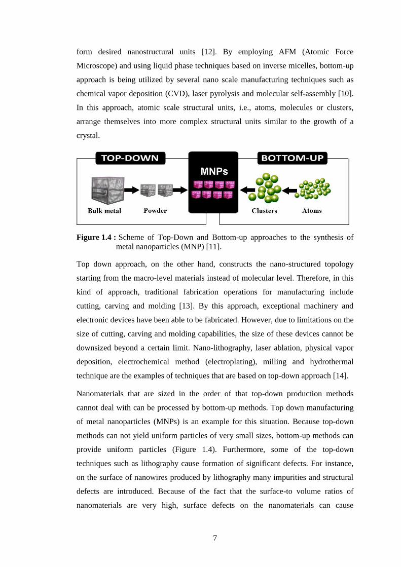
Figure 1.4 : Scheme of Top-Down and Bottom-up approaches to the synthesis of

metal nanoparticles (MNP) [11].

Top down approach, on the other hand, constructs the nano-structured topology

starting from the macro-level materials instead of molecular level. Therefore, in this

kind of approach, traditional fabrication operations for manufacturing include

cutting, carving and molding [13]. By this approach, exceptional machinery and

electronic devices have been able to be fabricated. However, due to limitations on the

size of cutting, carving and molding capabilities, the size of these devices cannot be

downsized beyond a certain limit. Nano-lithography, laser ablation, physical vapor

deposition, electrochemical method (electroplating), milling and hydrothermal

technique are the examples of techniques that are based on top-down approach [14].

Nanomaterials that are sized in the order of that top-down production methods

cannot deal with can be processed by bottom-up methods. Top down manufacturing

of metal nanoparticles (MNPs) is an example for this situation. Because top-down

methods can not yield uniform particles of very small sizes, bottom-up methods can

provide uniform particles (Figure 1.4). Furthermore, some of the top-down

techniques such as lithography cause formation of significant defects. For instance,

on the surface of nanowires produced by lithography many impurities and structural

defects are introduced. Because of the fact that the surface-to volume ratios of

nanomaterials are very high, surface defects on the nanomaterials can cause

8

considerable change in the surface properties [11]. Despite this disadvantage, top-

down engineering methods constitute an important place together with the bottom-up

chemistry in the development of nanoscience and nanotechnology.

In the perspective of nanoscience, every element in the periodic table, depending on

the desired target material, can be utilized in the manufacturing of nanomaterials.

Increasing control on the manufacturing of single nanostructural units that are

designed for specific purposes after their assembly into larger structures,

nanotechnology will enable us to synthesize revolutionary materials. In this way,

metals, ceramics or polymers can be manufactured in nano precision exactly without

machining.

1.2 Introduction to Nanoporous Materials

Like the CNTs and CNT based materials, nanoporous (np) materials are also

attractive research fields in nanoscience and nanotechnology. Nanoporous materials

are generally characterized as nano scale solid materials that include porous topology

in the length scales less than 1µm [12]. Materials categorized as np materials consist

of nano scaled cellular structure through which open channels or empty spaces exist,

which directly affect the behavior of np materials.

Large amount of nanoporous materials already exist in nature, especially in

biological systems and in minerals. For example, walls of biological living cells are a

kind of nanoporous membranes which include significant complexities due to their

responsibilities in living organisms. Besides that, some of the nanoporous materials

have found industrial applications for many years. Zeolites are the most known

nanoporous material, which have been employed in petroleum industry as a catalyst

for decades. Although the zeolites used in industry were natural, now most of them

are synthetic. As the progress achieved in nanotechonology to manipulate and

visualize objects at nanoscale, ability to control pore size of these materials at

nanoscale has been increased. By this way, creation of nano membranes having

controllable molecular structures with atomistic perfection can be realized. As the

size and composition of the nanoporous structure can be modified, its physical and

chemical properties can also be altered in a desired way.

9

Nanoporous materials show different functionalities according to the properties of

nanopores such as their shapes, sizes and amounts. Conventionally, pores are defined

as the voids or holes with different shapes (e.g., cylinders, balls, slits, hexagons,

spheres, etc. ) in a solid material. Pores may exist as isolated cells or interconnected

with each other through holes on the cell walls.

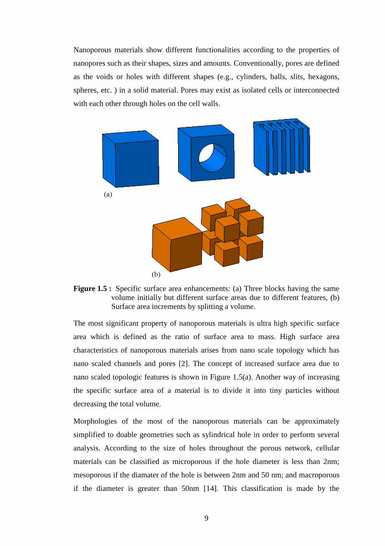
Figure 1.5 : Specific surface area enhancements: (a) Three blocks having the same

volume initially but different surface areas due to different features, (b)

Surface area increments by splitting a volume.

The most significant property of nanoporous materials is ultra high specific surface

area which is defined as the ratio of surface area to mass. High surface area

characteristics of nanoporous materials arises from nano scale topology which has

nano scaled channels and pores [2]. The concept of increased surface area due to

nano scaled topologic features is shown in Figure 1.5(a). Another way of increasing

the specific surface area of a material is to divide it into tiny particles without

decreasing the total volume.

Morphologies of the most of the nanoporous materials can be approximately

simplified to doable geometries such as sylindrical hole in order to perform several

analysis. According to the size of holes throughout the porous network, cellular

materials can be classified as microporous if the hole diameter is less than 2nm;

mesoporous if the diamater of the hole is between 2nm and 50 nm; and macroporous

if the diameter is greater than 50nm [14]. This classification is made by the

10

international scientific community (The International Union of Pure and Applied

Chemistry, IUPAC) to reach an aggreement on the classification of pores. Figure 1.6

illustrates some examples regarding this classification. Furthermore, examples of

microporous, mesoporous and and macroporous materials are given in Table 1.1.

Figure 1.6 : Three different types of nanoporous silica materials. (a) A microporous

material: zeolite, (b) A mesoporous material, (c) A macroporous material

[13].

The existence of pores within a material brings extra useful properties that do not

exist in the corresponding bulk material that do not have porous network. Porosity is

defined as the ratio of the empty space to the total volume of the material and usually

this value is between 0.2 and 0.95 for porous materials [15].

Examples of microporous, mesoporous and macroporous materials [16]. Table 1.1 :

Microporous

materials

Zeolite-like materials, activated carbon fibers (ACF),

templated carbon from zeolites, metal organic frameworks

(MOFs)

Mesoporous

materials

Mesoporous oxides (silica, alumina, zirconia), MCM-41,

CMK-1, polymeric materials

Macroporous

materials Porous glass, nanoporous silicon

Hybrid porous

materials

Activated carbon (AC, silica gel, pillared clay, nanoporous

oxide-bridged carbon nanosheet composites)

Pores within a porous material can be open or closed state. Open pores are an

interconnected network of the pores, but in case of a closed pore system, pores are

not interconnected with each other and at the isolated condition. Therefore, in

applications such as catalysis, filtration and adsorption, porous materials with open

pore architecture are much more favorable instead of porous systems with closed

pores. On the other hand, closed pore systems are preferable in sonic and thermal

insulation or lightweighted structural applications.

11

1.2.1 Properties of nanoporous materials

Due to their novel structural properties and large interconnected internal surface at

atomistic scale, the usage of nanoporous materials as catalysts and absorption media

is increasing day by day. Beside this, owing to their capacity to absorb and interact

with atoms and molecules, porous materials have significant importance in

nanoscience and nanotechnology [17].

Basic properties of nanoporous materials can be depicted as long as their microscale

characteristics are understood. In this regard, atomistic simulations such as molecular

dynamics simulations play an important role in supporting experimental studies.

As the porosity, pore size, pore size distribution and composition of nanoporous

materials vary, their pore and surface properties also change that also cause changes

in their potential applications. For different applications, a candidate material should

satisfy different set of requirements. For instance, to be a good absorbent, a material

should have several performance parameters such as high adsorption capacity, high

selectivity, good mechanical properties and acceptable stability and durability. High

adsorption capacity is mainly drived by the properties of specific surface area,

chemistry of surface and pore size which dictate the amount of materials collected by

unit mass of adsorbents. Similarly, selectivity property which is especially required

in case of a target of separating a desired material from a multi-component mixture,

depends highly on the pore size, shape and pore size distribution in addition to the

type of absorbates. The other required property is excellent mechanical properties

which help absorbers to resist attrition, erosion and crushing in adsorption columns.

In addition to these, due to abrasive chemical and thermal enviroments, stability and

durability of absorbent materials are very critical to sustain their functionality in long

terms. Several factors affect the degree of satisfying these requirements for

nanomaterials such as manufacturing methods and processing conditions.

1.2.2 Major opportunities in applications of nanoporous materials

The main advantage of nanoporous materials is their cellular structure at the nano

scale. Due to their porous nanostructure, they have a ultra-large surface area in

addition to controllable cell size and morphology. As mentioned previously, because

of their ultra-fine porous morphology, their material properties are superior in

comparison with their bulk counterparts. For that reason, extraordinary properties of

12

nanoporous materials enable them potenatial candidates in wide range applications

including photonic crystals, bio-implants, sensors and separators. Application areas

of nanoporous materials can be divided into two categories in which nanoporous

materials are employed as a bulk material form and membrane form. Generally

separation related applications make use of membrane type nanoporous materials

whereas bio-implants, sensors and photonic crytals are corresponding to the bulk

nature of nanoporous materials.

The most exciting point of membrane-type nanoporous materials is due to their

capacity of allowing certain sizes of objects to pass through the membrane while

other objects cannot pass. As the size of the cells within the nanoporous membranes

are controlled, control on the size of the objects that are targeted to eliminate can also

be controlled. Zeolites which are crystalline porous materials are known to be one of

the most popular nanoporous materials that have been used for separation purposes

for a long time. As observed in zeolites, three dimensional cellular network structure

of nanoporous materials offers very advantegous medium for selecting and

separating different molecular types.

One of the most important feature of nanoporous materials is their ultra large surface

areas as mentioned repeatitively in the text. Such a huge surface area results in high

sensitivity to alterations in the environmental conditions such as temperature, light

and humidty. Due to this advantage, nanoporous materials are widely used as sensors

and actuators.

1.3 Introduction to Carbon Nanotubes

Carbon is the essential element of life, because of the fact that its organic compounds

take parts in every living tissue. One of the reasons for its diversity in compounds is

the reality that carbon atoms have the ability to combine with other carbon atoms as

well as with other elements. Figure 1.7 shows the different structural forms of carbon

in nature. Carbon nanotubes (CNTs) which are shown as the allotropes of carbon

element are one of the fascinating examples of carbon based nanomaterials and can

be considered of as the sheet of graphite (graphene) rolled up into a seamless

molecular cylinder.

13

Figure 1.7 : Different structural forms of carbon element (a) diamond, (b) graphite,

(c) Lonsdaleite (hexagonal diamoond), (d) Buckminster-Fullerene (C60),

(e) C540, (f) C70, (g) amorphous carbon, (h) Nanotube [8].

The CNTs can have a length-to-diamater ratio greater than 106 making them an ultra

high aspect ratio material. Their diameter varies between 1 to 100 nm with a length

of up to several micrometers or even milimeters. The CNTs can be classified into

two major groups as single-walled carbon nanotubes (SWNT) and multi-walled

carbon nanotubes (MWNT). The SWNTs consist of only one layer of graphene sheet

while the MWNTs can be considered as the rolled stack of several graphene sheets.

Although discovery of the SWNTs are undisputedly clear, discovery of the MWNTs

is controversial. Regarding the SWNT, two papers [15,16] which were published

independently in the same year (1993) introduced the SWNTs into the scientific

research area. In case of the MWNTs, the first report giving the TEM images of

nanodiameter carbon fibres was published by Radushkevich and Lukyanovich in

14

1952 in the Journal of Physics and Chemistry of Russia in Russian. Because of cold

war, this report was not known by many scientists in the world. Therefore, many

people consider Iijima’s paper [17] published in 1991 as the first introduction of the

MWNTs into the research community.

Bulk sythesis of the SWNTs is relatively more difficult than the MWNTs due to

proper control requirement on the growth and atmospheric condition. Beside that

catalyst is required for the synthesis of the SWNTs while not needed for MWNTs.

Moreover, purity of the MWNTs are higher than SWNTs.

The CNTs are regarded as the one of the promising materials for the 21st century due

to their exceptional physical properties. Owing to these novel properties, the CNTs

have many potential applications in nanotechnology.

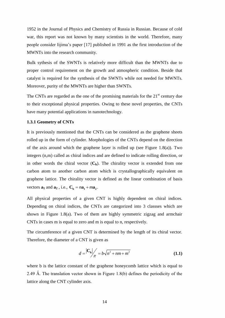
1.3.1 Geometry of CNTs

It is previously mentioned that the CNTs can be considered as the graphene sheets

rolled up in the form of cylinder. Morphologies of the CNTs depend on the direction

of the axis around which the graphene layer is rolled up (see Figure 1.8(a)). Two

integers (n,m) called as chiral indices and are defined to indicate rolling direction, or

in other words the chiral vector (Ch). The chirality vector is extended from one

carbon atom to another carbon atom which is crystallographically equivalent on

graphene lattice. The chirality vector is defined as the linear combination of basis

vectors a1 and a2 , i.e., n m h 1 2

C a a .

All physical properties of a given CNT is highly dependent on chiral indices.

Depending on chiral indices, the CNTs are categorized into 3 classses which are

shown in Figure 1.8(a). Two of them are highly symmetric zigzag and armchair

CNTs in cases m is equal to zero and m is equal to n, respectively.

The circumference of a given CNT is determined by the length of its chiral vector.

Therefore, the diameter of a CNT is given as

2 2d b n nm m

hC

(1.1)

where b is the lattice constant of the graphene honeycomb lattice which is equal to

2.49 Ǻ. The translation vector shown in Figure 1.8(b) defines the periodicity of the

lattice along the CNT cylinder axis.

15

Figure 1.8 : (a) Different rolling directions on a graphene sheet causing different

chiralities, (b) General geometric parameters for CNTs [18].

In a perfect CNT structure, all covalent bonds excluding the tip bonds are on the

hexagonal lattice system. However, during the synthesis process, defects are formed

and pentagonal, heptagonal bonds and other imperfections occur, which lowers the

quality of the CNTs.

1.3.2 Manufacturing of CNTs

Several techniques have been used for the synthesis of carbon nanotubes including

arc discharge, laser ablation, high-pressure carbon monoxide disproportionation

(Hipco) and chemical vapor deposition (CVD). Procesess for the generation of the

CNTs in many of these methods are realized in a vacuum or with process gases. On

the other hand, the CVD synthesis of the CNTs can be in vacuum or at atmospheric

pressure. As the techniques used in catalytic or continous growth processes are

advancing, commercialization of CNT products becomes feasible.

The quality of the CNTs generated by catalytic techniques is not as good as the ones

synthesized by the arc-evaporation method in which a catalyst is not utilized.

However, despite this disadvantage catalytically manufactured CNTs have received

great attention following IIjima’s paper in 1991 [17] due to several reasons. The

most important reason behind this popularity is the capacity of catalytic methods to

produce scaled-up CNTs, in other words susceptibility of massive production.

Therefore, bulk synthesis of the CNTs by employing catalytic methods is possible,

which in turn creates popularity on them. Secondly, controlled growth of the CNTs

on the target substrates can be managed by catalytic methods, which is highly

16

applicable especially in display technology. In this regard, the CVD is the dominant

technique for the high-volume CNT production.

1.3.3 Applications of carbon nanotubes

Ranges of diamaters for the SWNTs and MWNTs are usually 0.8 to 2nm and 5 to

20nm, respectively. However, sometimes diameters of the MWNTs can exceed

100nm. On the other hand, the maximum length scale of the CNTs starts from the

values less than 100 nm and reach up to several centimeters which is the macroscale

range [19].

The tensile strength value measured for an individual MWNT is 100 GPa which is 10

times higher than any industrial fiber. Depending on the chirality, the SWNTs can be

metallic or semiconducting while the MWNTs are usually metallic and can carry

currents up to 109 (A/cm

2). Beside this, thermal conductivity of a SWNT based on

the wall area is around 3500 (Wm-1

K-1

) which is higher than the thermal conductivity

of diamond [15].

Even though scientific research on the CNTs exploided in 1990s following the first

industrial synthesis of CNTs, substantial growth in the commercial area has observed

in the last decade. Following the year 2006, the capacity of CNT production has

increased 10 times and growth of research study numbers on CNT related subjects

continue [16].

Today, most of the CNTs which are bulk produced is employed in composite

materials and thin films, and topology of these CNTs is randomly organized rather

than being in a specific order. However, ordered CNT structures such as vertically

aligned forests, yarns and sheets have very high potential to be used in shape

recovery, dry adhesion, high damping, terahertz polarization, large stroke actuation

and thermoacoustic sound emission [20-22].

It should be noted that CNT macrostructures such as yarns and sheets possess

considerably lower mechanical, thermal and electrical properties than those of

individual CNTs. Usage of the MWNTs are more favorable than the usage of the

SWNTs where diameter and band gap of the CNTs are not so important, because of

higher prices of SWNT production. The reason behind this higher cost is that

synthesis of SWNT by the CVD needs to be controlled by tighter process parameters

and high cost of research and development of process. Thus, the SWNTs that have

17

controlled the chirality can be favorably employed in the emerging applications if the

prices can be cut down.

First usage of the MWNTs was in plastics as a electrically conductive filler due to

their ability of forming a light percolated network with a 0.01 weight percentage. By

using disordered MWNTs in polymers to form CNT-polymer composites,

conductivity of overall composites can be increased to 10000 (S m-1

) at a weight

percentage of 10. These electrically conductive light plastic composites are used in

automotive industry to sustain electrostatic- assisted painting of mirror housings and

also in the fuel lines and filters to ensure dissipation of electrostatic charge. These

CNT polymer composites are also utilized in electromagnetic interference (EMI)

shielding packages and wafer carriers in microelectronics industry [21].

Figure 1.9 : CNT composites and macrostructures (a) Micrograph showing the cross

section of a carbon fiber laminate with the CNTs dispersed in the epoxy

resin and its application. (b) CNT sheets and yarns used as lightweight

data cables and electromagnetic (EM) shielding material [23].

The CNT reinforced polymer composites are also used as a solution to lighweighted

structural applications. For this purpose, the CNT powders are added into polymeric

resins to elevate stiffness, strength and toughness properties effectively. For example,

adding only approximately 1 weight percentage of the MWNTs into epoxy resin

18

improve the stiffness and fracture toughness by 6 and 23%, respectively [24]. In the

meantime, this amplification does not yield any degradation on the other mechanical

properties. The CNT reinforced composites can also present good damping

characteristics due to stick-slip mechanisms between the CNTs themselves and the

contact between CNT and polymer. Due to its enhanced damping capacity, the CNT

composites are used to improve sporting goods such as tennis racquets, baseball bats

and bicycle frames.

The CNT based resins are also utilized to upgrade fiber composites. This

enhancement has recently been used for lightweight wind turbine blades and hulls of

maritime boats. In this regard, Figure 1.9(a) shows a cross section of a composite

fiber laminate that consists of dispersed CNTs in the epoxy resin and a sample

application is given as maritime security boats of which boat hull is made by

lightweighted CNT fiber reinforced composites [25].

For high technology applications where lightweight solutions together with

multifunctional capabilities such as combined mechanical and electrical functionality

are required, a serious competition is expected to be observed between the CNT

yarns and laminated sheets produced by the direct CVD and carbon fiber (see Figure

1.9(b)).

1.4 Purpose of Thesis

The main purpose of this dissertation is mainly to develop efficient algorithms to

generate representative atomistic models of randomly organized nanostructures

which were selected as CNT network and nanoporous materials and to employ those

atomistic models in molecular dynamics simulations for investigating the mechanical

behavior of selected nanomaterials. Both CNT networks and nanoporous materials

have complex geometries formed by random networks of carbon nanotubes and

ligaments, respectively. Thus, generating their computational atomistic models is a

very challenging issue that should be solved to realize numerical experiments. In this

regard, as the first step of the dissertation, stochastic models have been developed for

random natured CNT network materials and nanoporous materials. The other

purpose of this dissertation is to open a way that other researchers can employ the

algorithms that are developed within this study, in other studies for the investigation

19

of randomly organized nanostructures. In this perspective, it is aimed to develop

tools or methods that can be used in future studies.

Due to lack of efficient algorithms that can be used in the modeling of randomly

organized nanostructures, i.e., CNT networks and nanoporous materials, there are a

few studies in literature regarding mechanics of these materials. Therefore, the other

main purpose of this study is to examine mechanical behavior of CNT networks and

nanoporous materials by using the atomistic models generated by the techniques

which are developed in the first stage of the dissertation. In this perspective, the

ultimate goal of this dissertation is to get deep understanding of the deformation

mechanisms in CNT network and nanoporous materials. It is important to have

essential information about the dependence of mechanical performance on the

topological features, in order to manufacture outstanding novel materials. Therefore,

in the scope of this dissertation, numerical experiments are conducted by molecular

dynamics simulations to provide the relationship between topological parameters and

mechanical properties.

21

2. OVERVIEW OF MOLECULAR DYNAMICS SIMULATIONS

As mentioned before in the previous chapters, molecular dynamics (MD) simulations

have been utilized to investigate mechanical behavior of nanostructured materials in

this dissertation. In this regard, this section presents an overview of molecular

dynamics (MD) method and related subjects.

2.1 Introduction

Numerical experiments, namely computer simulations, are important tools, today, in

scientific research and development efforts. In history, real experiments and

theoretical work were the main frames escalating the progress in science. In an

experimental study, the system under investigation is subjected to specific boundary

conditions and measurement of parameters that are in question are obtained and

numerically stored. In a theoretical work, a physical system is represented by

governing mathematical equations consisted of driving parameters of the system. In

order to validate the mathematical model formed in theoretical study, the stability or

predictive capacity of the model should be shown by several simple cases that would

allow solvable mathematical equations. However, for the sake of getting solvable

mathematical equations, many times complexities of the system disappears which

take us away from the real world problems.

Formerly, theoretical models were able to be examined only in limited special cases.

For example, in condensed matter physics, intermolecular forces within a selected

material could be justified in a diatomic molecule or in a perfect and infinite lattice

crystal system. Even under the simplified conditions, further approximations were

usually demanded to perform calculations. However, many of physical issues that

fall into the both academic and practical interest, such as physics and chemistry of

defects, surfaces, organic molecules and so on, cannot be simplified to be

investigated by theoretical models.

22

High speed computers that appeared in the 50s introduced a new player, numerical

experiments, in the scientific research area in addition to experiments and theoretical

studies.

Figure 2.1 : Examples of nanostructures that can be simulated by MD (a)

Nanowires, (b) Carbon nanotubes, (c) Bio-molecules [26].

In numerical experiments or in other words computer simulations, a theoretical

model that governs the simulation still exists but the calculations are performed

numerically by high speed computers under the framework of algorithms developed

in an appropriate computer language. By numerical experiments, much more

complicated phenomena can be injected into the numerical system, which guide

towards investigations of more realistic systems.Numerical simulations conceptually

23

stand at a position between experiment and theory. The models employed in the

computer simulations are just numerical models, not the real physical system, which

translates the computer simulations concept towards theory. On the other hand,

validation of a numerical model is much more like a real physical experiment in the

way of evaluation of simulation results, which conveys the computer simulation

concept towards experiments.

In the past, interactions between atoms were calculated by two-body potentials which

have uncomplicated analytical forms, e.g., Morse or Lennard-Jones potentials. At

present, however, many body potentials, which are obtained numerically by using

forces anticipated by first-principle methods, are the examples of much more precise

potentials.

Moleculare dynamics (MD) method is a computer simulation method to obtain the

time trajectories of an ensemble of atoms, which interact with each other, by

performing numerical integrations of equations of motions. It is a very effective

technique to investigate atomic scale and macroscale properties of nanomaterials

such as naowires, carbon nanotubes or bio-molecules as shown in Figure 2.1.

In MD simulations, atoms are considered as a point mass that are linked by springs.

In this idealization, springs represent the bonds between atoms. Force fields, or in

other words, potentials are utilized to obtain the time trajectory of atomic positions

and velocities.

Molecular dynamics method utilizes the law of classical Newtonian mechanics,

named as Newton’s 2nd

Law, for the derivation of equations of motion:

i i imF a (2.1)

Equation (2.1) is defined for each atom i that exists in an atomic system consisted of

N atoms. In this equation, im is the atomic mass, 2 2

i id dta r is the acceleration

and iF is the force acting on the ith

atom resulting from the interaction with other

atoms around it. Thus, unlike Monte Carlo method, which basically depends on

random sampling of solutions to get numerical results, molecular dynamics is a

deterministic method in which the atomic phase space variables at the current time

step are calculated by using previous time step.

24

Trajectory of atoms is calculated in a 6N-dimensional phase space consisting of 3N

positions and 3N momenta. Because molecular dynamics is a statistical mechanics

method, similar to Monte Carlo method, the MD is employed to attain some of the

phase configuration that is distributed based on a statistical distribution function, or

statistical ensemble. For example, microcanonical ensemble corresponds to a

probability density function that fixes the total energy, E. In macrocanonical

ensemble, from the infinite number of states, only states that have a certain energy

(E) are selected. It is shown as by dirac function, H E . In this representation

H and represents the Hamiltonian and phase space variables (positions and

momenta), respectively. So, phase variables are selected so that the Hamiltonian is

equal to the specific energy. Another example of statistical ensemble is the canonical

ensemble in which the temperature parameter is constant and Boltzman function,

exp / BH k T , is used as the probability density function.

In statistical physics, based on a selected statistical ensemble (e.g., canonical or

microcanonical) for a specific quantity, there exists an infinite number of

configurations distributed according to the corresponded ensemble. The physical

quantities are identified as the averages over the configurations. Atomistic

trajectories established by molecular dynamics simulations are considered as the set

of configurations satisfying the ensemble conditions. In this regard, physical

quantities can be measured by MD simulations easily by arithmetic averages of

values taken at several instants.

Statistical physics maintains the connection between the microscopic properties and

thermodynamic properties of a physical system. In theory, it is expected that for

infinite simulation times, the phase space obtained by the MD simulation will be

completely cover all configurations and the averaging operations will yield

thermodynamic properties at that limit time. However, in practice, simulation times

are always limited to a finite length, therefore it should be carefully examined

whether sufficient sampling has been done or not. By this way, measurement of

thermodynamic properties and evaluation of phase diagram of a certain material can

be achieved by the MD simulations.

In addition to molecular dynamics simulations, there are other traditional atomistic

simulation techniques such as quantum-mechanical methods in which Schrödinger

25

equation is numerically solved. Quantum mechanical methods are computationally

very expensive; therefore, they are combined with other methods to get accelerated

solutions. Beside to quantum mechanical simulations which are computationally very

intensive, faster simulation techniques such as Monte Carlo and coarse grained

models are also used to investigate atomistic structures.

2.2 History and Future of MD Simulations

Alder and Wainwright wrote the first academic paper in 1957 acknowledging

molecular dynamics simulation [27]. By employing a hard sphere system through

which interactions between the particles are defined as instantaneous collisions, they

investigated the solid and liquid regions of the phase diagram of the system. The

paper by Gibson et al. published in 1960 is one of the first studies that carry out

molecular dynamics simulations of a 500-atoms system utilizing continuous force

potentials with a finite difference time integration scheme to investigate the defect

generation by the impact of radiation damage [28]. In another well-known study by

Rahman in 1964, by using Lennard-Jones potential several properties of liquid Ar

were explored with a system consisting of 864 atoms [29].

By using MD simulations, defect formation and their effects on the mechanical

behavior in crystalline materials has been a popular subject for a long time [14]. In

recent years, investigations on the defects have focused on linear and planar defects

instead of point defects. As the potentials are getting improved to describe the

interactions between atoms, more realistic systems are being simulated.

Dynamic behavior of biomolecules such as proteins, nucleic acids (DNA, RNA) and

membranes, which are large macromolecules, can also be examined by molecular

dynamics simulations [30]. Because functional properties of biomolecules are highly

dependent on dynamical changes, the MD simulations are quite helpful to extract

dynamical response of biomolecules. The MD simulations are also actively

employed in pharmaceutical industry to effectively design of drugs.

In the last decade, by the development of Car-Parrinello method, which enables to

calculate interatomic forces by solving the electronic structure instead of using an

interatomic potential, electronic properties of materials can also be studied by the

MD simulations.

26

The most prominent advantage that the MD simulations provide to researchers is the

extraction of all properties about a thermodynamic system which is physically

possible to exist. However, the power of the MD is limited to computational power

and time-scale range that can be covered.

As the computational power increases day by day, more complex and so more

computational intensive problems can be solved numerically. Because the computers

are much cheaper than the laboratories, which provide the equivalent testing

opportunities, molecular dynamics simulations can save significant amount of money

in the development stages of new and novel materials and pharmaceuticals.

Figure 2.2 : Molecular device design examples (a) Gear chain [27] and (b) Planatary

Gear [27].

Theoretically, molecular structure of a material, which may be organic or inorganic,

can be designed in a numerical environment and its material properties can be

determined via computer simulation methods such as the MD simulations. By using

numerical specimens with different molecular structures, an optimum molecular

structure that satisfies required material properties can be obtained. Following these

numerical design iterations, proposed material can be synthesized in the laboratory

and further refinements can be done in the laboratory environment.

The approach and procedure summarized above have already been applied in the

design of new pharmaceuticals and are very close to being routinely employed in the

processing of polymer materials. Day by day this approach is increasingly being

realized in all material-related industries such as lubrication, catalysis, electronics

and chemical engineering. From this point of view, molecular dynamics simulation

method holds very important step to be taken towards novel materials or nano

27

electromechanical device design (see Figure 2.2). While its usage currently is limited

to academic field excluding a few areas such as pharmaceutical and polymer design,

in the next 20 years the MD simulation technique is estimated to take the place of

today’s computational tools , e.g., CFD or FEM in industry.

2.3 Limitations on MD

Although molecular dynamics method is a very useful and effective tool that helps

researchers to dive into the atomistic world, there are some limitations that need to be

addressed.

The first constraint on the MD technique comes from the usage of classical Newton’s

Laws instead of much more reliable Schrodinger’s equation that can capture the

quantum effects. It should be noted that the systems at the atomistic level are

governed by quantum laws rather than classical macroscale laws. Classical

approximation to the atomistic world can be verified by de Broglie thermal

wavelength [28] that was defined as

22

BMk T

(2.2)

where M, T, and Bk are atomic mass, temperature, Planck’s constant and

Boltzmann’s constant, respectively. The classical approach used in the MD can be

confirmed if a is much less than 1, where a is the mean nearest neighbor

separation. For the liquids of light elements (e.g., Li and Ar) which are at the triple

point that three phases (gas, liquid, solid) coexist at the same time, the ratio of a

is at the order of 0.1. This ratio decreases down for heavier elements. Therefore,

classical approximation is not confident for very light elements such as He and Ne.

Besides this, as the temperature of any system is adequately low, quantum effects

play much more important role which cannot be neglected. In these domains,

molecular dynamics simulations should be used with caution.

Another issue with the MD simulations is the calculation of forces. It will not be

wrong to state that the heart of an MD simulation is the calculation of forces.

Because the interaction between atoms results in the forces acting upon

corresponding atoms, which drive the motion of the atoms in the system, calculation

28

of forces on the atoms as accurate as is very important to capture the real physical

response. Forces are generally calculated by the gradient of a potential function

which is dependent on the coordinates of the atoms in the system. Therefore, the

degree of realism of the MD simulation highly relies on the capacity of the potentials

to capture the same response of the material under the boundary conditions that are

employed in the simulation.

Figure 2.3 : MD simulations workflow.

Molecular dynamics simulations are combined with statistical mechanics to extract

macro scale equilibrium (i.e., temperature, pressure and energy) and transport

properties (i.e., diffusion coefficient, shear viscosity and thermal conductivity) of a

classical many-body system. Figure 2.3 presents the major calculations that are

performed in the MD calculations. According to this, three basic steps form the main

framework of molecular dynamics. In the first step, initial positions and velocities for

each atom in the system are assigned. Then, the particles in the simulation box

commenced to interact with each other via a potential function and forces acting

upon each atom are calculated based on the potential used. For this reason, the

potential employed for the simulation is the key player to determine the degree of

realism of the simulation. Due to computational efficiency, potential calculations are

not performed between all atoms. Instead of that, by defining a radius of

Update neighbor list

Get forces

Solve equations of motion over

Perform p, T control (ensembles)

Calculate the desired physical quantities

? End Simulation

Set the initial conditions:

29

neighborhood, for each atom, only a number of atoms within the neighborhood are

used to determine interatomic forces.

In the second step, the Newton’s 2nd

law, i i imF a , is utilized to obtain velocities

and positions of atoms for the further time steps. Time evolution of atoms results in

the motion of atoms in the simulation box yielding a trajectory in space. In the third

step, position and momenta of atoms are used to determine physical quantities of the

system by profiting from statistical mechanics concepts. As stated above, according

to statistical mechanics, macro scale properties of a system is the average of the

corresponding quantity over all possible quantum states, which is called the

ensemble average. An ensemble can be considered as the fictive set of distinct

quantum states, all of which have the same macroscopic properties such as

temperature and pressure. In other words, for a defined system there exist different

quantum states (i.e, phase space of atomic system) satisfying the same macroscopic

properties. An ensemble is the collection of all quantum states that have same

macroscopic property. According to the Ergodic hypothesis which declares that the

ensemble averages of system properties are equal to time averages. Therefore, by

taking the time average of measurements obtained by the MD simulations,

macroscopic physical quantities can be achieved.

2.4 Time Evolution in MD Simulation

After assigning initial positions and velocities to particles, trajectory of the particles

are determined by integrating the equations of motion numerically. The classical

equations of motion can be written as

, , ,q G p r p F p r (2.3)

where H is the Hamiltonian, ,G p q H p and ,F p q H q . In classical

dynamics, the Hamiltonian has the general form

2

2

ii

i i

Um

p

r (2.4)

where ir and ip are the coordinates of the ith

atom and its momentum, respectively.

The first term of the Hamiltonian function, 2 2i imp represents the kinetic energy

30

while the second term, iU r is the potential energy resulting from the interatomic

interactions.

Because of the reason that the Newton’s 2nd

law does not depend on time, the

Hamiltonian function is also time independent. Furthermore, in the case of an

isolated system, the total energy that is the sum of potential and kinetic energies of

each atom is conserved.

The total time derivative of the Hamiltonian function given in Eqn. (2.4) is given as

Eqn. (2.5) considering that Hamiltonian is not explicitly defined by time, 0H t .

0i i

i ii i

dH H Hp r

dt p r

(2.5)

The total time derivative of Eqn. (2.4) for an isolated system is given in Eqn. (2.6).

1

0i i i

i i i

dH Up p r

dt m r

(2.6)

When the Eqns. (2.5) and (2.6) are compared, following relations can be realized:

ii

i

i i

pHr

p m

H U

r r

(2.7)

Substitution of Eqns. (2.7) into Eqn. (2.5) results in the following relation:

0 i i i

i i i

H Hp r p

r r

(2.8)

Thus, Hamiltonian equations of motion which are first order differential equation

with 6 degree of freedom can be written as follows:

i

i

i

i

Hr

p

Hp

r

(2.9)

There exist many different algorithms for the time evolution of particle dynamics

[29]. Here is given one of the basic algorithms to calculate the time history of

coordinates and momenta. In this regard, firstly the force is calculated in time-half a

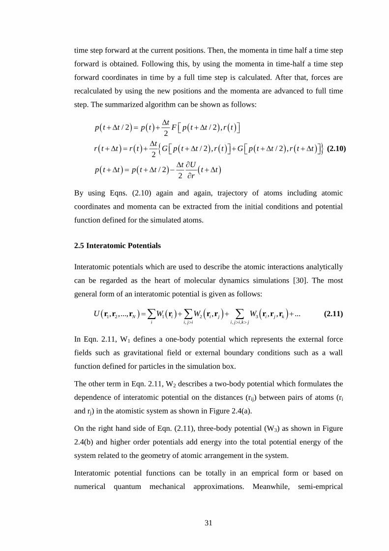
31

time step forward at the current positions. Then, the momenta in time half a time step

forward is obtained. Following this, by using the momenta in time-half a time step

forward coordinates in time by a full time step is calculated. After that, forces are

recalculated by using the new positions and the momenta are advanced to full time

step. The summarized algorithm can be shown as follows:

/ 2 / 2 ,2

/ 2 , / 2 ,2

/ 22

tp t t p t F p t t r t

tr t t r t G p t t r t G p t t r t t

t Up t t p t t t t

r

(2.10)

By using Eqns. (2.10) again and again, trajectory of atoms including atomic

coordinates and momenta can be extracted from the initial conditions and potential

function defined for the simulated atoms.

2.5 Interatomic Potentials

Interatomic potentials which are used to describe the atomic interactions analytically

can be regarded as the heart of molecular dynamics simulations [30]. The most

general form of an interatomic potential is given as follows:

1 2 1 2 3

, , ,

, ,..., , , , ...N i i j i j k

i i j i i j i k j

U W W W

r r r r r r r r r (2.11)

In Eqn. 2.11, W1 defines a one-body potential which represents the external force

fields such as gravitational field or external boundary conditions such as a wall

function defined for particles in the simulation box.

The other term in Eqn. 2.11, W2 describes a two-body potential which formulates the

dependence of interatomic potential on the distances (rij) between pairs of atoms (ri

and rj) in the atomistic system as shown in Figure 2.4(a).

On the right hand side of Eqn. (2.11), three-body potential (W3) as shown in Figure

2.4(b) and higher order potentials add energy into the total potential energy of the

system related to the geometry of atomic arrangement in the system.

Interatomic potential functions can be totally in an emprical form or based on

numerical quantum mechanical approximations. Meanwhile, semi-emprical

32

interatomic potential functions are also derived by parametrization of experimental

data and ab initio data. Force field calculations are the most time consuming part

within the MD simulations taking up to approximately 95% of the total simulation

time.

Figure 2.4 : (a) Two-body potential parameters, (b) 3-body potential parameters.

As mentioned before, setting up interactions between atoms or molecules correctly is

very important in terms of adding realism into the MD simulations. At the bottom

level, interactions are the product of quantum effects in which the electrons and

nuclei of atoms come into play. The relationship of electrons and nuclei is not same

by nature for different materials, which yields wide variety of behaviors. For

instance, in some materials atomic bonding type is covalent while for some other

materials it is ionic. However, in some other materials, the interaction type is

metallic where the electrons are free to walk around the nuclei without being belong

to a certain nucleus or shared by nuclei. As another extreme example in noble gases,

electrons are tightly stitched to atoms representing a close-shell structure [31,32].

Apart from these extreme examples, these different quantum behaviors can be

observed at different temperature and pressure conditions. For example, at room

temperature silicon material is structured as diamond which is a covalent semi-

conductor, while at temperatures higher than melting temperature ( 1670oK )

silicon material turns into metallic [33]. Similarly, at constant temperature increasing

pressure upon diamond material will cause a phase transition and results in a metallic

material.

In general, two different approaches can be classified for the adoption of interactions

between atoms and molecules. In the first approach, a potential function that depends

on the interatomic positions (i.e., relative distances and angles) and some parameters

33

which are fitted to map the actual properties of the system onto the potential function

[34]. In this approach, dynamics of electrons and behavior of electrons are not

directly included in the potential functions. However, in the second approach which

is theoretically more intellectual but computationally more expensive, electronic

structure is taken into consideration and forces on the atoms are calculated based on

quantum mechanical behavior. This second approach is the baseline of ab initio

molecular dynamics simulations.

Classical molecular dynamics is based on the first approach; thus, the forces on the

atoms are derived from the gradients of the potential function with respect to

displacements:

, ,i i

i i i i

U U UU

x y z

F r

r (2.12)

As mentioned before, in MD simulation techniques it is very important to employ

appropriate interatomic potential that will provide proper interaction forces between

the atoms in the system. In this regard, force models are the most computationally

intensive parts of a molecular dynamics simulation code, taking up to 95% of the

total simulation time [36].

2.5.1 Pairwise interactions

As the simplest case, the interatomic potential can be represented as the sum of

pairwise interactions:

1 1

N N

ij

i j

U u r

(2.13)

where ,ij i j ij ijr r r r r and the summation condition 1j avoids the summation

of double interactions.

2.5.2 Lennard-Jones potential

Lennard-Jones potential whose formulation is given below is one of the most well-

known potential utilized for Van der Waals system and initially offered to be used

for Argon (see Figure 2.5).

34

12 6

4LJ ij

ij ij

u rr r

(2.14)

Lennard-Jones potential is the function of two parameters such as is the scaling

parameter that adjusts the magnitude of the energy (so can be called as energy-scale

parameter) and is a length-scale parameter which affects the change of potential

as the atomic distances change [37]. These parameters are selected to fit the certain

physical properties of the system.

Figure 2.5 : Lennard-Jones potential [33].

Lennard-Jones potential is especially suitable for closed-shell materials such as Neon

and Argon liquids where the electrons are confined to each atomic nucleus; therefore,

for open-shell systems where strongly localized bonds are observed; it is not fully

satisfactory [38].

2.5.3 Embedded atom method

Embedded atom method (EAM) is a semi-emprical model for the description of

interatomic interactions and deals with each atom in the simulation box as being

embedded in a host lattice environment which is comprised of all other atoms [39].

In this method, the total energy of a pure metal system consisting of N atoms is given

by the following relation:

N

tot i

i

E E (2.15)

35

where iE , energy term for the ith atom in the system is calculated by the following

relation which consists of two terms.

1

2i ij i

j

E r F (2.16)

where the first term ijr represents the atomic pairwise interaction between atoms

is a function of atomic displacements and the second term iF that is also named

as embedding energy function represents the effect of electron density of the

environment in which the atom is embedded. The embedding energy function

depends on local electron density which is calculated as the summation of

pairwise interaction terms ijr :

i ij

j

r (2.17)

Because of the reason that the actual forms of ijr , ijr and F are not known

exactly, their parameterized forms are used [37]. The coefficients of the

parameterized functions are obtained by fitting to already known properties such as

the lattice parameter, cohesive energy and elastic constants.

2.5.4 Adaptive intermolecular reactive emprical bond-order potential

Adaptive Intermolecular Reactive Emprical Bond-Order (AIREBO) Potential

developed by Stuart et al. [40] potential is an empirical potential that is used to

model interactions between Carbon and Hydrogen. This potential is an extended

version of the Brenner’s Reactive Emprical Bond-Order (REBO) potential [41] and

non-bonding atomic interactions are included. The basic formula for the AIREBO

potential is given by

REBO LJ torsE E E E (2.18)

As it can be inferred from Eqn. (2.18), the AIREBO is compound of Reactive

Emprical Bond Order REBOE , Lennard-Jones Potential LJE and torsional

potential torsE .

The Reactive Emprical Bond Order REBOE part of the AIREBO is a short range

potential and represents the covalent bond interactions.

36

REBO R A

ij ij ij ij ijE V r b V r (2.19)

In Eqn. (2.19), R

ijV and A

ijV represent the repulsive and attractive pairwise potentials

and ijb is the bond-order term. Several chemical concerns such as the existence of

neighboring atoms and type of hybridization which affect the condition of covalent

bonding interaction are elucidated in this term.

Lennard-Jones potential term (i.e., LJE ) employed in the AIREBO potential is

expanded in Eqn. (2.20). It consists of conventional Lennard-Jones potential term

LJ

ijV as well as sine (S) and cosine (C) switch functions.

* 1LJ LJ LJ

ij r ij b ij ij ij ij r ij ij ij ijE S t r S t b C V r S t r C V r

(2.20)

where 12 6

4ij ijLJ

ij ij ij

ij ij

V rr r

Torsional potential term torsE given by Eqn. (2.21) depends on dihedral angle that is

produced by four neighboring atoms and includes cosine switches varying from 0 to

1.

, , ,

10

1

2

256 1cos

405 2 10

tors tors

ij ij jk jk kl kl ijkl

i j i k i j l i j k

tors

E w r w r w r V

V

(2.21)

In this study, the EAM and AIREBO potentials have been used for the MD

simulations of nanoporous metals and carbon nanotube networks, respectively.

2.6 Overview of LAMMPS

The LAMMPS (Large-scale Atomic/Molecular Massivle Parallel Simulator)

developed by a cooperative research consortium consisting of two US Department of

Energy (DOE) labs and three companies, is an open source classical molecular

dynamics code specially tuned for multi-core computer clusters [26]. By using the

LAMMPS, several nanoscale systems such as atomic, polymeric, biological,

metallic, granular and coarse-grained systems can be modeled with a large library of

force field potentials.

37

Systems with only a small number of particles to millions or even billions of

particles can be modeled by the LAMMPS and the models can be run on any parallel

machine on which C++ compiler works.

While the earlier versions of the LAMMPS was written in F77 and F90, latest

versions of the LAMMPS have been written in C++. Because its programming

design has been adapted to be updated by others, researchers can easily modify the

code and extend its abilities by adding new force fields, atom types or boundary

conditions.

The LAMMPS has a large interatomic potential library including potentials for soft

materials (i.e., biomolecules, polymers), solid-state materials (e.g., metals, semi-

conductors) and coarse grained or mesoscopic systems. Other than atomistic systems,

in a general manner as a particle simulator, the LAMMPS can also be employed to

simulate any systems that consist of discrete particles, and interactions between

particles are described by potentials.

In a common point of view, the LAMMPS realize the numerical integration of

Newton’s equations of motion for a set of atoms, molecules or macroscopic particles

which are in interaction with each other by short or long range forces under several

boundary conditions. In order to maintain a computationally efficient solution

scheme, the LAMMPS employs neighbor lists to perform force field calculations and

these neighbor lists are optimized for systems consisting of particles which are

repulsive at short distances. In that way, elevation of local density of particles is

avoided. In parallel runs, spatial-decomposition method is utilized to divide the

simulation domain into smaller domains that are individually assigned to individual

processors.

39

3. ATOMISTIC MODELLING AND MECHANICS OF NANOPOROUS

MATERIALS

3.1 Introduction

Nanoporous materials are one of the classes of nanostructured materials, which

already exist in nature both in bulk and membrane forms. Biological cell walls are

good examples of nanoporous membranes, which have the ability to permeable

selectively owing partially to their nanoporous morphology. As a bulk nanoporous

material, zeolites have been used as catalysts in industry for many years. In the

recent years, artificial nanoporous (np) materials are also manufactured with precise

control on the morphological parameters including pore size, distribution, porosity

and chemical properties [42]. Due to their extraordinary physical and chemical

properties such as ultra high surface-to-volume ratio, exceptional electrocatalytic

ability, strain reversibility and high yield strength, nanoporous materials are highly

attractive candidates for medical application devices, i.e., bioartificial organs,

implantable drug delivery systems, also for lighweighted structural applications,

energy absoption devices and heat sinks [43].

In general, for nanostructured materials the target is to scale down the bulk materials

into nanometer scale. However, for nanoporous materials the major interest is the

scaling down the pore volume, i.e., empty space within the bulk material instead of

bulk material that encapsulates the pore volume. Most of the important practical

features of nanoporous materials arise from their structural network of pores, which

enable them prominent candidates in applications such as adsorbing,

accommodating, sieving and separating molecules. For this reason, nanoporous

materials are different than other nanostructured materials due to that the functional

properties of nanoporous materials are significantly affected by the characteristics of

nanopores or nano cells such as pore size, shape and intensity in addition to the

surface and bulk properties of constituent materials.

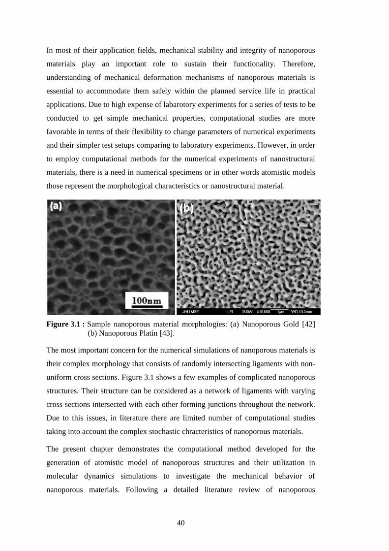
40

In most of their application fields, mechanical stability and integrity of nanoporous

materials play an important role to sustain their functionality. Therefore,

understanding of mechanical deformation mechanisms of nanoporous materials is

essential to accommodate them safely within the planned service life in practical

applications. Due to high expense of labarotory experiments for a series of tests to be

conducted to get simple mechanical properties, computational studies are more

favorable in terms of their flexibility to change parameters of numerical experiments

and their simpler test setups comparing to laboratory experiments. However, in order

to employ computational methods for the numerical experiments of nanostructural

materials, there is a need in numerical specimens or in other words atomistic models

those represent the morphological characteristics or nanostructural material.

Figure 3.1 : Sample nanoporous material morphologies: (a) Nanoporous Gold [42]

(b) Nanoporous Platin [43].

The most important concern for the numerical simulations of nanoporous materials is

their complex morphology that consists of randomly intersecting ligaments with non-

uniform cross sections. Figure 3.1 shows a few examples of complicated nanoporous

structures. Their structure can be considered as a network of ligaments with varying

cross sections intersected with each other forming junctions throughout the network.

Due to this issues, in literature there are limited number of computational studies

taking into account the complex stochastic chracteristics of nanoporous materials.

The present chapter demonstrates the computational method developed for the

generation of atomistic model of nanoporous structures and their utilization in

molecular dynamics simulations to investigate the mechanical behavior of

nanoporous materials. Following a detailed literature review of nanoporous

41

materials, the philosophy behind the atomistic modeling of nanoporous structures is

presented by explaining the basic steps of the algorithm. It has been successfully

shown that the morphology of nanoporous structures consisting of intersecting

ligaments can be formed under spherical cell shape assumption by controlling the

porosity. The main idea of the presented algorithm is the generation of ensembles

consisting of randomly intersected spheres under certain constraints including

maximum number intersections per one sphere and amount of intersection of two

spheres. It is also illustrated that the generated foam models resemble conventional

cellular structural units such as the ligaments with a non-uniform cross section

distribution, junctions at which a number of ligaments are joined and pores on the

cell walls with diameters controlled by certain parameters within the algorithm. After

providing detailed explanations regarding the atomistic modeling process, results of

molecular dynamics simulations performed on the atomistic nanoporous models with

different porosity values are presented. According to those molecular dynamics

simulations, it is found that softening of an open cell nanoporous structure subjected

to tensile loading can be significantly reduced when the size of ligaments and the

joints that connect them in the structure is designed to be sufficiently small. It is

found by using molecular dynamics simulations that the softening becomes slightly

slower with increasing the porosity for the structures with porosity less than or equal

to 72%, and stress localization is observed during softening. In contrast, for

structures with more than 75% porosity, the softening is much slower, and stress

delocalization occurs during softening. It is argued that at relatively high porosity,

the softening is governed by both the ligament size and joint size because their

compliance becomes high enough to allow the overloading stress due to ligament

rupture to be redistributed more effectively throughout the structure.

3.2 Literature Review

Nanoporous materials have been vigorously studied over the past decade. They have

caught researchers’ attention primarily for chemical characteristics such as catalysis,

adsorption, filtration and sensing [42–48], but recently investigations have begun on

their mechanical properties. The very low relative density of np materials makes

them intriguing candidates for lighter materials in many different applications.

However, the decrease in density is accompanied by a decrease in several important

42

material properties, including stiffness, strength [43] and ductility [44]. The

decreases in stiffness and strength are expected because of scaling laws [45] and, in

fact, the decreases are less than predicted due to the surface effects [45-47] and size

effects [48]; so at present the need is greatest to understand and improve the loss of

ductility in np materials. Several theories exist to explain macroscopic brittleness,

including the possibility of a narrow ligament size distribution [49] resulting in

failure of a large percentage of ligaments at once. In the same vein, a statistical

average of ligament size overestimates the ability of the entire ligament network to

carry the stress [50] since the weakest link of the minimum ligament size initiates the

failure throughout the structure as the stress concentrations intensify. In this study,

we present encouraging results of simulations to show that softening of nanoporous

materials decreases at large porosities by the diffusion of stress among the entire

structure, rather than concentration of stress at failure nucleation sites.

Since the popularity of np materials has increased in recent years, many experimental

and theoretical studies have been devoted to investigate the properties of nanoporous

materials. Many of these studies focused on np-Au material due to its unique

properties and ease of manufacturing.

As an experimental study, Hodge et al. [45] performed nano-indentation tests to

investigate the correlation between the yield strength, relative density and ligament

sizes of open-cell nanoporous foams. Utilizing np-Au samples with different relative

densities and ligament sizes, they constructed a Hall-Petch-type relation between the

yield strength and ligament size by modifying the Gibson and Ashby’s yield strength

equation derived for open-cell macrocellular foams [42].

Recently published two papers [46, 47] focused on the mechanical properties of

nanoporous gold (Au) materials by using atomistic MD simulations. In both studies,

open-cell microstructure of nanoporous gold material is obtained by employing the

phase field method which mimics spinodal decomposition of a binary fluid mixture

of two constituents. Farkas et al. [47] investigated both tensile and compressive

response of nanoporous numerical test samples and reported a significant

tension/compression asymmetry in the yield strength, which was explained by the

initial compressive state of the system emerging from surface stresses that favors the

compression. Importantly, they also observe densification of the foam with the

amount of ~15% under tensile deformation of 30%. This densification is interpreted

43

as the result of decrease in pore diameter that realizes by plastic deformation of

ligaments.

Sun et al. [48], on the other hand, performed only uniaxial tensile simulations

preferring to concentrate on the atomistic physical mechanisms behind tensile

deformation of nanoporous gold. They reported the formation of stacking fault

accumulations along the tension direction in the ligaments and at the ligament

junctions together with the Lomer-Cottrell locks at the junctions. Modifying Gibson

and Ashby’s scaling law of the Young’s modulus derived to link the bulk Young’s

modulus and foam Young’s modulus, Sun et al. presented a relationship between the

effective Young’s modulus and relative mass density of nanoporous materials.

3.2.1 Theoretical and semi-emprical models for macroporous foams

Cellular solids, or commonly foams, can be defined as the assembly of three

dimensional randomly distributed cells which are constructed by interconnected

struts and/or plates. Struts enclosing the cells are beam-like structural members and

intersect with the other struts to form the main frame of a cell. Intersections of struts

form the vertices or junctions in the cellular solids. Cellular solids are classified as

open cell and closed cell foams according to the material distribution along the edges

of the cells. In the open cell foams, cells are interconnected with each other and

plate-like faces closing the faces of the cell do not exist. In contrary to open cell

foams, cells throughout the closed cell foams are not interconnected with each other

due to plate/shell like walls between the cells. The material properties of cellular

solids basically depend on the base material that establishes the foam structure, the

relative density, mean cell diameter and the type of the foam (i.e., closed cell or open

cell) [42]. In this dissertation, main focus is on the open cell cellular materials due to

that most of nanoporous metals have interconnected open cell architectures. The

book “Cellular Solids” by Gibson and Ashby [42] provides a solid background on the

experimental and theoretical studies on macroporous (mp) solids.

In literature, there are numerous theoretical studies for the modeling of macroporous

foams. Using repetitive idealized unit cell models to get homogenized behavior of

foams is one of the techniques that have been employed in literature so far. These

idealized unit cells used to set up cellular networks are selected to be in different

shapes such as cubic [46], tetrakaidecahedral [49], tetrahedral [50] or bubbles [51].

44

In most of these micromechanical models, initial elastic constants (i.e., the Young’s

modulus E*, shear modulus G

* and Poisson’s ratio ν

*) have been aimed to be

captured by the unit cell models considering the ligaments of the cells as structural

beams and employing the descriptions of elastic constants in the classical strength of

materials. One of these unit cell models to account for the mechanical properties is

the widely employed cubic unit cell model developed by Gibson and Ashby [42]. In

this cubic unit cell model, the scaling equations that maintain a relationship between

the Young’s modulus, yield strength and relative density of the foam are provided as

follows:

2* *

1

S S

EC

E

(3.1)

3* 2*

2

pl

ys S

C

(3.2)

where * and S represent the density of the foam and density of the bulk solid

material of which the foam is made, respectively. In the same manner, *E and *

pl

are the Young’s modulus and yield strength of the foam respectively, while SE and

yl are the Young’s modulus and yield strength of the solid material, respectively.

As it can be noticed from Eqns. (3.1) and (3.2), the key parameter that governs the

mechanical properties of macro porous foams is the relative density of the foam

*

S . In this regard, as the relative density decreases the general trend is the

cutback of the mechanical properties such as the stiffness, strength and ductility [52-

53]. The coefficients 1C and 2C in Eqns. (3.1) and (3.2) are established to be equal

to 1 and 0.3 [46], respectively, by adjusting the equations to the experimental data. It

should be noted here that Eqns. (3.1) and (3.2) are valid for foams with low relative

density values. The basic deformation mechanism at low relative density or

equivalently at high porosities is the bending of cell walls [48, 52]. As the relative

density increases, the modified material distribution around the cell walls results in

different mechanical properties [48]. The yield strength equation, Eqn. (3.2), that is

applicable for high porosities was modified by Gibson and Ashby to include

45

corrections for the description of mechanical behavior of foams at higher relative

density values as follows:

13* 2* * 2

2 1pl

ys S S

C

(3.3)

In general, macroporous metallic foams demonstrate three distinguishable

deformation stages under compressive loading. The first regime is controlled by the

bending deformation mode of cell walls and forms a linear elastic region in parallel

to conventional stress-strain curves. By its classical definition, the Young’s modulus

of the foam *E can be calculated at this regime as the slope of the linear curve. The

next stage following the linear elastic region is the long plateau region in which the

cell wall bending deformation mechanisms ceased and collapsing of cells occurs.

After this plateau regime, the final stage presents a sudden stress increase and

densification of the foam. Densification is resulted from the collapsing of the cell

faces upon each other and so is a sign of destruction of the cells to transform a solid

material without any void. Therefore, the slope of the stress-strain curve at this

regime is equal to the Young’s modulus of the solid material of the foam; in other

words, during compression loading of a cellular solid, the characteristic is dominated

by the demolition of the cells foam structure transforms into the bulk solid material.

3.2.2 Experimental studies on nanoporous foams

Practical usage of cellular materials in some cases results in a requirement of

mechanical stability of the material as in the cases of actuators and sensors.

Therefore, investigations on the mechanical behavior of open cell nanoporous

materials are vital to improve their role in the practical appplications. In literature,

there is an abundant number of experimental studies focusing on the yield strength

and elastic modulus of nanoporous materials. The values reported in these studies for

the yield strength and elastic modulus were shown to vary from 11MPa to 240MPa

and 3GPa to 40Gpa, respectively [39, 53-56]. Within the comparisons between

nanoporous gold (Au) and bulk Au, it is shown that nanoporous Au may be stronger

than its bulk counterpart of which the yield strength depends on the load history and

ranges between 10MPa to 200 MPa [56-61]. This superiority of nanoporous Au over

46

its bulk counterpart may enable a new class of material to show up itself in the high

strength materials area.

Nanoporous (np) materials demonstrate a completely distinct behavior than their

bulk counterpart materials. As an example to this important phenomena is that

although bulk Au material show a ductile fracture failure under tensile loading,

nanoporous form of Au presents a brittle behavior under tensile stresses. In addition

to that, nanoporous materials exhibit typical properties of porous materials under

both compressive and tensile loading. However, the scaling Eqns. (3.1) and (3.2)

developed for the prediction of the Young’s modulus and yield strength of macro

porous materials are not applicable to nanoporous materials, which directed

researchers to investigate new scaling equations to describe nanoporous materials.

As mentioned previously, Eqns. (3.1) and (3.2) that were developed by Gibson and

Ashby were derived by directly comparison of experimentally measured Young’s

modulus or yield strength values at different relative density values. These equations

can be used for all types of open cell macro porous foams disregarding the material

types.

Indendation tests are one of the popular experimental methods to realize

measurements for cellular solids. Generally, for bulk materials the hardness values

(H) obtained from indentation test are related to the yield strength values as ~ 3H

relations [62]. On the other hand, this relationship between the hardness value and

yield strength for cellular solids with the low relative density * 0.3S is

assumed to be ~H relations [63]. Under a compressive loading, a cellular solid

does not expand in the directions transverse to the loading direction; therefore,

effective Poisson’s ratio is assumed to be approximately zero. Indentation tests are

also applied at nano scale by taking the name of nanoindentation and similar to

macroscopic case the relationship between hardness value and yield strength is

defined as ~H relations.

One of the first experimental studies on nanoporous materials performed by Rong Li

and K. Sieradzki [53] was focused on the ductile to brittle transition in nanoporous

Au. They showed that as the ligaments get thinner they do not behave in brittle

manner. In another study, Khang et al. had reported that ratio of the specimen size to

the element strength distribution at random porous structures plays a significant role

47

on the ductile-to-brittle transition [64]. In their study, Li and Sieradzki employed

nanoporous Au that was specified as “highly porous” gold and concluded that their

study would be a sample system for the determination of physical properties in the

future works.

Following those studies mentioned above, by using different methods, mechanical

properties of nanoporous materials have been studied. The majority of the studies

performed on the nanoporous Au employed the nanoindentation techniques to

determine the mechanical properties, i.e., the yield strength and Young’s modulus. In

this regard, in the next sub-sections, the first review is given on the elastic modulus

of nanoporous materials under compressive loading. After that, experimental studies

which had utilized nanoindentation tests to study the yield strength properties is

discussed. In the meantime, the results obtained through other techniques than

nanoindentation is presented. Finally, the literature review was performed

considering the studies that were focused on the tensile properties of nanoporous

materials.

3.2.3 Studies on the Young’s modulus of nanoporous materials

Based on the results obtained from the studies on the elastic modulus of nanoporous

materials, as the sample or microstructural geometry size decreases, an

accompanying decrease in the Young’s modulus is not an anticipated behavior [52].

In this regard, Volkert et al. [65] carried out a series of uniaxial compression tests on

nanoporous Au columns by using test specimens with different diameters to

investigate the effect of sample size on the elastic modulus. They determined the

Young’s modulus as 7 GPa by using the unloading portion of the true stress-strain

curve of the samples under small plastic strain [66]. Beside this, elastic modulus of

nanoporous Au was determined by Biener et al. [67] to be in the same order of

magnitude by employing nanoindentation tests with depth sensing. The Young’s

modulus of nanoporous Au obtained by several experimental techniques can be

compared with the analytical predictions that could be provided by Eqns. (3.1) and

(3.2). For this purpose, the Young’s modulus of single crystal Au which is in the

range of 57-85 GPa [56] and porosity value of 36 % or relative density of 0.64 were

used as input values into Eqns. (3.1) and (3.2). As a result, scaling equations yielded

elastic modulus values of 7-11 GPa which match well with the experimental results

48

obtained from [67] and [68]. Moreover, in the outcome of experimental studies, no

dependency of measured Young’s modulus on the specimen sizes was noticed.

However, in contrast to the results obtained from the studies [66] and [56] that were

mentioned above, in the study performed by Hodge et al. [45], they found out

inconsistency between their experimental Young’s modulus measurements, that were

measured for foams with relative density in the ranges of 0.25 to 0.41, and analytical

results calculated by the scaling equation in which the relative density exponent is

equal to 2, i.e., n=2. On this issue, they provided an explanation saying that primary

reason behind this inconsistency was that scaling equations developed by Gibson and

Ashby were valid for foams with low relative density where the size of ligaments are

less than the size of pores. On the other hands, the foams employed in their

experiments with relative density ranges of 0.25-0.41, ligament and pore sizes are

comparable to each other, which results in considerable contribution of ligaments

into the overall deformation mechanism [68].

Another conflicting result was obtained by Mathur and Erlebacher [60] on the issue

of size effects on the elasticity modulus. In their study, their results indicated that the

Young’s modulus of the nanoporous structure is influenced from the microstructural

length scale changes. They reported that when they decreased the ligament size from

12nm to 3nm, four times less than the initial values, they observed four times

increase in the Young’s modulus of nanoporous Au. They used a buckling based

method for the mechanical testing of stress free nanoporous Au films through which

ligament sizes range from 3nm to 40nm. According to their results, size dependency

of elastic modulus is much more apparent when the ligament sizes are smaller than

10nm. For the ligament sizes larger than 10nm, the effect of size dependency is not

as considerable as the ligament sizes less than 10nm. Comparisons made between the

Young’s modulus values obtained from nanoindentation measurements [69-71] and

values calculated by Gibson and Ashby scaling equation, Eqn. (3.1) resulted in good

agreement for the ligament sizes larger than 12nm of nanoporous Au. Four times

increase in elasticity modulus of nanoporous Au films in case of ligaments smaller

than 10 nm was explained by several factors such as surface stress effect. Another

explanation was related with the morphology of the nanoporous structure stating that

porous networks consisting of smaller size ligaments contain large number of

ligaments comparing with porous networks having larger ligaments, so less

49

ligaments. As a result of increasing number of ligaments, total bending stiffness of

the porous network became larger than the network consisted of larger ligaments.

However, these results are not incompatible with the other experimental findings

which reported that the elasticity modulus of nanoporous materials is not affected

considerably by size effects [72]. For instance, in the experimental study given in

Ref. [73] it has been shown that elastic modulus of both Au nanowires, which

represent the ligaments of nanoporous Au, and bulk Au material do not depend on

the diameters of specimens.

So far all the studies given here are related with the dependency of elastic modulus of

nanoporous materials on the size effects. In addition to these studies, there are also

studies investigating the effects of residual contents within the nanoporous structure.

For example, in one of these studies [74], effects of residual Ag content on the

Young’s modulus of nanoporous Au materials were investigated. They noted that

during the de-alloying process of Au-Ag alloy, in order to generate ligaments smaller

than 30nm, diameter surface diffusion should be suppressed which causes an

increase in the concentrations of residual Ag content. As a result of increasing

amount of residual content, density of the yielded material also increases, which in

turn causes the Young’s modulus to increase. This change in the Young’s modulus

due to the density increase can also be deduced from the Gibson and Ashby’s scaling

equation, Eqn. (3.1), which indicates that an increase of relative density will also

provoke the raise of the Young’s modulus of any kind of foam. In the guideline of

the results obtained in this study, stiffening effect of ligaments smaller than 12nm

that was observed in Mathur and Erlebacher’s work [60] can also be explained by the

existence of residual content in small sized ligaments.

3.2.4 Studies on the yield strength of nanoporous materials

Previously it was mentioned about that indentation had been proven to be an

acceptable method to measure the yield strength of macro porous foams. However

several concerns including the densification and indentation size effects should be

handled to verify this measurement technique. For the densification issue, both

nanoporous and macroporous foams face with a similar case in which the area of

porous media contacting with indenter is compressed and densified locally while the

other regions outside the indenter diameter range are not affected from the

densification [75]. In the study presented by Andrews et al., several indentation tests

50

were conducted on macro porous aluminum (Al) foams to show the indentation size

effects [76] and effect of sample size with respect to the cell size on the mechanical

behavior was investigated. According to the results obtained by this study, a decrease

in hardness values was observed in the form of an exponential function which has

variables of cell size and indenter size. Similar results were reported by Hodge et al.

[68] for nanoporous Au in the case of nanoporous materials. Andrews et al. [76] also

reported that the yield strength values extracted from both compression and

indentation tests for low density macro porous foams are comparable with each

other. In the same manner, for the verification of nanoindentation tests, Chen et al.

[77] provided validation of nanoindentation method by comparisons between

nanoindentation test results with the results from bulge test measurements. They also

presented another comparison between nanoindentation results and finite element

solutions of mechanical response of thin nanoporous polymer films and showed that

the values were in good agreement [77].

Experiments conducted via nanoindentation tests on nanoporous materials with low

relative density pointed out the high strength capability of nanoporous foams. In one

of those studies, namely Biener et al. [71], nanoporous Au specimens with 0.42

relative density and ligament length of 100nm were utilized in hardness

measurements and hardness values obtained as a result of experiments were 10 times

higher than the hardness values estimated by the scaling equation developed by

Gibson and Ashby. They also demonstrated by the SEM (Scanning Electron

Micrograph) images which are shown in Figure 3.1 that the type of governing

deformation mechanism in a nanoindentation test realized on nanoporous Au is

ductile or in other words plastic densification. Likewise, Volkert et al. [66] used

ligaments of nanoporous ligaments with 15 nm length and established that the yield

strength of those ligaments are close to the strength values of bulk gold material. For

that purpose, they first determined the hardness value of 100 MPa through an

experimental stage and then this hardness value is substituted into the scaling

equation, Eqn. (3.2) with the relative density of 0.36. As a result, the yield strength of

individual ligaments of nanoporous Au material predicted as 1.5 GPa which is in

good agreement with the anticipated theoretical shear strength of Au which presents

a state in which the neighbor atomic layers slide on another plane without the effect

of dislocations [78].

51

Figure 3.2 : SEM micrographs of 8000-mN indentations on a fractured surface of np

gold: (a) conospherical tip with a tip radius of 0.1 mm, and (b)

Berkovich tip with a curvature of 200 nm. Ductile densification is

observed for both probes. Note that the plastic deformation is confined

to the area under the indenter, and adjacent areas are virtually

undisturbed [5].

High yield strength results obtained from the nanoindentation tests, which were

mentioned above, was a surprising outcome of the experimental studies comparing

with the results related with size effects which were expected to play much more

important role in the mechanical behavior of nanoporous foams. In this regard,

studies reported in the last years provided a thorough illustration of sample and grain

size effects on the plastic deformation response of nanostructured materials.

Dominant role of size effect on the mechanical characteristics of materials at nano

length scale were demonstrated via both experimental studies and numerical

simulations (e.g., molecular dynamics). For instance, Hodge et al. [68] investigated

the dependency of the yield strength of nanoporous Au foams on the microstructural

length scale by performing nanoindentation tests on the samples with relative density

values ranging from 0.2 to 0.42. Figure 3.2 shows their comparison made between

their experimental results with the values calculated via scaling equation given by

Gibson and Ashby. It can be inferred from the figure, that as the ligament size

decreases, the yield strength of np-Au having the same relative density also

decreases. This result is in contradiction with the results provided by other studies on

macro porous foams in which the ligament size is greater than 1.0µm and the

predictions determined by the scaling equation of Gibson and Ashby which do not

include the size effect dependency of mechanical properties for a fixed relative

density. As the size of ligaments gets closer to 1.0µm, the results obtained from

nanoindentation experiments converge to the values calculated by the scaling

equation.

52

Figure 3.3 : Experimental values for foam yield stress for samples of np Au with

relative density ranging from 20% to 42%, normalized by the yield

stress of fully dense Au. The solid line presents the Gibson and Ashby

prediction for a gold foam [79].

Effect of ligament sizes on the yield strength of nanoporous materials was also

studied by Hakamada et al. [58] by carrying out nanoindentation tests of nanoporous

Au speciemens that were manufactured by dealloying method. By using the

experimental results, they formed a relationship between the yield stress and

ligament sizes as follows:

m

ys Kd (3.4)

where d , K and m represent the ligament size, a constant and the power of size

dependency, respectively. The value of m in Eqn. (3.4) is determined as -0.20 from

the plot obtained by experimental results. This value obtained for m shows

similarities with the values in analogous equations developed for the face centered

cubic (fcc) metallic nanowires [79] in literature, which can be deduced that the

deformation mechanisms in both cases are also comparable with each other. Upon

this deduction, in their study, Hakamada et al. [58] mentioned that several

microstructural alterations due to size effects observed in fcc metallic nanowires such

as a decrease in the number of defects in grains, the repression of emission and

53

reabsorption of dislocations may also be resulting mutational mechanisms due to the

length scale effects.

On the other hand, still there is not a certain agreement about the length scale

dependent governing mechanisms that drive the deformation modes of nanoporous

Au together with nanowires and columns of Au. Despite the lack of such a consensus

on this issue, most of the studies in literature followed the path of comparing the

results belong to the mechanical behavior of ligaments in np-Au with the results of

columns and nanowires of Au. In the studies [80] and [81], experimental results

provided by indentation tests on nanoporous Au and nanomechanical measurements

conducted on submicron Au columns and nanowires were evaluated. Dependency of

the yield strength to the length scale as discovered in nanoporous Au was also

observed for the micropillars or nanowires of Au. As a matter of fact, the yield

strength values of microcolumns and nanowires which have very small crystal

structures yielded very high values. Moreover, in another study reported by Geer and

Nix [82] the length scale dependency of the yield strength established in np-Au was

proved to exist also for submicron Au columns and concluded that theoretical yield

strength could be maintained as the diameters of Au columns were reduced below a

few hundred nanometers.

In the study performed by Volkert and Lilleodden [67] micropillars of Au which

were made from large grained Au sheets using a focused Ga+ beam were subjected to

nanoindentation tests to measure the yield strength. Based on the experimental

results, an exponential law, nd

describing the relation between the yield strength

and the diameter of columns, d employed in the experiments similar to Eqn. (3.4)

was derived. The exponential term of this relation, n was found to be 0.61. Because

these results are in good agreement with the relationship between the yield strength

and ligament diameter which was also observed by Eqn. (3.4) for np-Au, it can be

concluded that the deformation mechanisms of nanoporous Au and micropillars of

Au may have similarities.

Explanation of the length scale effect on the mechanical properties of nanostructured

material is attributed to the existence of free surfaces which confines the number of

dislocation nucleations. Biener et al. [72] in their study noted that because the

ligaments of nanoporous-Au are related to the Au microcolumns, as the size of the

ligaments decreases within nanoporous-Au, the stress values at which the

54

dislocations are activated to move increase as well until the theoretical shear strength

is reached. In this regard, their results indicating the dependency of nanoporous Au

to the length scale effects are in the same scope with the results obtained from

compression tests performed on micro columns of Au. Several factors such as

modified internal stress fields, changes on the active dislocation size and number of

dislocation sources are shown as the reasons of increasing of dislocation activation

stress [83]. Many of the studies which demonstrated that the yield strength of

ligaments in np-Au approaches the theoretical shear strength are also satisfied with

this explanation provided for micro columns of Au; therefore, Biener et al. [67]

referred nanoporous Au as the three- dimensional network of defect free ultra high

strength Au nanowires.

All the studies given so far mentioned about similarities between deformation

mechanisms of nanoporous Au and Au nanowires or microcolumns. However, in the

study presented by Dou and Derby [70] showed that the deformation mechanisms of

these two nanostructure groups may differ from each other. In this regard, in order to

focus on micro-mechanisms of deformation in nanoporous Au ligaments, they

investigated the deformed structure following an indentation by using the TEM.

According to their results, they reported that there was no considerable distinction

between the results obtained by the use of np-Au ligaments and 3D macroscopic

samples due to that the deformation mechanisms of both np-Au ligaments and bulk

np-Au consisted of comparable ligament sizes are similar. According to the studies

performed by Gibson and Ashby, it had been suggested that due to localized plastic

deformation at the intersection of ligaments, namely junctions, plastic collapsing of

macro porous foams occured by bending of ligament. With this conclusion reported

by Gibson and Ashby, localized plastic deformation through ligament bending also

observed by surface steps noticed in the TEM images presented in the study of Dou

et al. [84]. Moreover, around the junctions where the ligaments are met, Shockley

partial dislocations and micro twins were observed to exist. However, in the

deformed structure of np-Au ligaments, no perfect dislocations were found, which is

compatible with strengthening models based on strain gradient hardening [84]. Strain

gradient hardening models are basically continuum scale deformation mechanisms-

based models claiming that geometrically essential strains block further deformation

yielding a strengthening effect on the mechanical behavior of the material. The TEM

55

images provided by Dou et al. [84] demonstrated the generation of complex

microtwins by propagation and interaction of Shockley partial dislocations. They

also claim that the basic difference between the compressive deformation

mechanisms of nanowires and np-Au ligaments is the primary bending mode

observed in nanoporous structures.

Figure 3.4 : The load-displacement curve recorded during in-situ TEM

nanoindentation of a 150 nm np-Au film. It appears that the load drops

(marked by arrows) corresponding to collective collapse of a layer of

pores [67].

One of the experimental techniques that is exhibited in the last years and named as

in-situ nanoindentation method was utilized by Sun et al. [46] to study on the

deformation mechanisms of nanoporous Au thin films. In their study, they used np-

Au thin films 150 nm in thickness consisting of ligaments with diameters in the

range of 10 to 20 nm [46]. As noted, they investigated the microstructural

characteristics of deformation by employing the TEM during the operation of

nanoindentation. By this way, they had visualized the deformation process, and so by

using the TEM images they stated that in the initial phase of nanoindentation,

deformation of np-Au was noticed to occur readily by compressing of the ligaments

just under the indenter while the rest of the structure below this region stayed

56

uncompressed. In the further time of the nanoindentation process, as the indenter

moves forward, head of the compressed region moved in front of the indenter

resulting in collapsing of neighboring ligaments.

Two local maximum points which are separated approximately by a distance of size

of a pore on the displacement versus load curve as shown in Figure 3.3 indicate the

compression and then collapsing of a layer of cells in which the ligaments enclosing

the cells buckle, at the same time yielding a sudden decrease in the load value

applied by the indenter. In addition to that, by the help of the TEM images tracing of

dislocations showed that dislocations spanned the ligament width. It was also noticed

that the transportation of dislocations throughout the ligaments and at junction

regions where the ligaments are intersected, dislocations are entangled with other

dislocations coming from other ligaments.

Although there are huge amounts of studies focusing on the size effects and high

yield strength characteristics of nanoporous materials, there are limited numbers of

studies which presented the strain hardening properties of nanoporous materials. The

main reason for this is the difficulty of evaluating the complicated strain history

generated by nanoindentation technique. In the most of the experimental research,

nanoindentation method is employed due to its simplicity compared with other

mechanical testing methods. However, as a result of nanoindentation test, complex

strain history avoids interpretation of strain hardening characteristics of the material.

Figure 3.4 shows the true stress-strain curve of np Au ligaments obtained through

uniaxial compression tests, which were demonstrated by Volkert et al. [67]. As it can

be inferred from Figure 3.4, there is a substantial strain hardening behavior of

nanoporous Au columns, which approaches approximately two times of the yield

strength progressing up to 30% strain. It is also noticed that each strain hardening

region is followed by a plastic flow region.

By using thin nanowires of np-Au through nanoindentation tests, strain hardening

characteristics of np-Au were also studied in Ref. [85]. In this study, strain hardening

property observed even at small strain values was attributed to the contacts between

the ligaments of high relative density foams.

Nano pillar micro-compression testing technique is another experimental method that

is less complicated than nanoindentation test for the measurement of nanoporous-Au.

57

In their study Biener et al. [61] performed uniaxial compression tests of np-Au

columns by using the procedure provided by Uchic et al. [86]. Micro columns of Au

specimens employed in that study were manufactured by focused ion beam technique

with approximate length-to-diameter ratio of two. Strain hardening behavior of the

micro columns was not captured from the true stress-strain curve in which a constant

flow stress was observed following approximately 2.5% strain (see Figure 3.5). On

the other hand, as also obtained in nanoindentation measurements, in the

compression tests carried out in this study yielded high yield strength values, which

in turn indicates that the type of the testing method is not the reason behind the

results of high yield strength values of np-Au.

Figure 3.5 : True stress-strain curves from 1, 4 and 8 μm diameter nanoporous Au

columns [66].

Even though there are many studies having reported the remarkably high yield

strength of nanoporous Au that were presented in the previous paragraphs, there are

also some other studies which demonstrated considerably different values of yield

strengths. For example in Ref. [87], the obtained value of yield strength for np-Au is

approximately one order less than the values reported in the studies where

nanoindentation experiments were performed on the samples. In that study, np-Au

samples were generated by a different method that was introduced by Jin et al. [88].

58

In general, dealloying manufacturing method yields np-Au samples which show

unexpected mechanical failures due to their volumetric shrinkage tendency such as

stress corrosion cracking and brittle fracture [89]. Crack formation during

manufacturing of nanoporous Au was able to be avoided and thus crack free samples

were able to be manufactured by Jin et al. [88]. Because the volumetric shrinkage

percent during the manufacturing process is less than 2%, their samples were crack

free. Their compression test results showed that their samples exhibit outstanding

ductile behavior in the way that without any fracture almost all of the structure was

able to be compressed. Plastic deformation distribution across the sample section was

shown to be homogenous by electron backscatter diffraction (EBSD) maps, which

conflicts with conventional observation of deformation bands propagating through

the sample. The other discrepancy of this study is the low yield strength values that

are not consistent with other studies which had employed nanoindentation tests for

the yield strength measurements and equated the yield strength value to hardness

value ~H for only low density foams [89].

The other reason underlying the noticeable distinct results may be due to the

manufacturing method which causes different morphology formation. Their micro

structure formed by a long-range coherent crystal lattice system where each grain

consists of billions of nano ligaments that have the same set of crystallographic slip

planes [90]. From their EBSD maps, it was observed that during the deformation

process the grain structure of the ligaments did not change which was evaluated as

that a collective shear of ligaments occurred along shared slip planes and in the same

directions contrary to the known low density foams [91]. The other studies is worth

being mentioned in this section considered that macroscopic strength of nanoporous

materials could be driven by the joint relation of relative density and size dependency

of ligaments; however, in this study another aspect of deformation mechanism which

is the interrelated deformation of individual ligaments, was presented to be

accounted for the understanding of deformation mechanism of np materials.

3.2.5 Studies on the Tensile Behavior of Nanoporous Materials

Number of studies on the tensile fracture behavior of nanoporous materials is not too

many in comparison with the number of studies on the compressive deformation

behavior. Brittle tensile characteristics of Au-Ag alloys under corrosive conditions

59

had been demonstrated in the earlier studies [92] focusing on the stress corrosion

crack formation on Au-Ag alloys. The results presented in these studies were

consistent with the film-induced cleavage model according to which crack generation

is encouraged by the formation of thin layer of np-Au during the dealloying process

and propagation of the crack is through the new formed dealloyed layer towards not

corroded bulk material [93]. As mentioned before, although bulk Au material

exhibits ductile fracture characteristics in tensile loading, it has been demonstrated

that macroscopic tensile failure mode of np-Au materials is remarkably brittle [94].

Due to this brittleness of np-Au materials, handling of np-Au test specimens were

reported to be so difficult. In addition to those, Li and Sieradzki [63] presented that

considerably larger test specimens comparing with their ligament/pore size yield

more brittle fracture behavior. Because of these properties of nanoporous materials,

their tensile mechanical testings are very challenging to perform.

Dealloying process of nanoporous metals causes high ratios of volume shrinkage as

well as tensile built stresses embedded into the structure [95]. As the content of Ag in

the Ag-Au alloy that is employed in the dealloying process increases, the degree of

brittleness of the structure also increases. For instance, samples generated from

Ag80Au20 alloys by dealloying are quickly fail to keep their structure without

destruction due to inherent tensile stresses from dealloying process, while the

samples generated from Ag70Au30 alloys survive their integrity. The study [96]

performed on the nanoporous Au nanowires that were made from Ag82Au18 (i.e.,

with high content of Ag) established a significant result which stated that nanowires

as well as nano thin films are more resistant to tensile built stresses that emerge due

to dealloying process than their macroscale counterparts, because of the reason that

their volumetric shrinkage is not very effective.

Biener et al. [71] in their detailed study conducted three-point bending tests to

investigate the fracture characteristics of np-Au. It was observed that test specimens

were catastrophically failed in the tensile stress region rather than compressive zone

following a crack propagation phase, showing that the structure is more susceptible

to compressive loadings. Because there was no traceable plastic flow before the

failure, it was concluded that the failure of the material occurred after a crack

propagation phase which is in brittle nature. On the other hand, ductile failure of

individual ligaments through nanoporous Au was presented by the SEM images of

60

the microstructure showing the necking behavior due to plastic deformation. Besides

these, MD studies on Au nanowires [71] demonstrated that elongation of ligaments is

100%, which was an expected result due to that gold is the most malleable metal.

As also reported by an earlier study by Khang et al. [64] for a random network

model, macroscopic brittleness is considered to be the result of narrow ligament-

strength distribution through the network. Based on their explanation to the brittle

behavior, failure of the weakest ligament initiates the crack propagation in the

network of ligaments by causing extra straining and overloading of closest ligaments.

The route of the crack propagation is the direction in which the resistivity of the

structure is the lowest. Therefore, Khang et al. [65] defined the total strength of the

network as the largest critical defect resulting in the highest stress concentration. As

stated in Ref. [72], amount of Ag component increase in the grain boundaries of Ag-

Au alloy that would be used in the dealloying process activates the generation of

higher porosity material while creating 2D like voids. These voids are the root cause

of the crack formation and then propagation due to elevated stress concentrations. In

this content, they noted that the mechanical behavior of np-Au could be enhanced by

introducing wider ligament strength distribution.

In another study [97], test specimens were tested within a customized testing setting

and comparable fracture behavior of np-Au could be obtained through a serial

experimental work. In this study, digital image correlation (DIC) method was utilized

to perform strain measurements, which makes it possible strain measurements

without any contact with the capacity of full-field advantage. In addition to those,

this method of which the details are provided in [98] also enables the calculation of

the Poisson’s ratio. Due to macroscopic brittle behavior of nanoporous Au

deformation, test specimens did not show any plastic flow in tensile loading.

Following the initial elastic phase in the tensile deformation, a crack initiation and

then propagation phase is ceased by a quick failure which occurs on the plane

perpendicular to the tensile loading axis indicating the brittle fracture behavior. As it

can be noticed from the SEM images they provided, they also stated the plasticity of

the individual ligaments causing the ductile failure of the samples. The plastic

deformation of the ligaments was reported to be considerably localized due to that

neighbor ligaments stayed intact while 1 or 2 ligaments that are in the crack surface

region are subjected to plastic deformation. This phenomenon was explained in their

61

study by the situation that ligaments cannot store the dislocations which move to the

surface and then escape.

3.3 Atomistic Modeling of Nanoporous Materials

In this section, complexity of nanoporous structures are introduced and then the

algorithm developed to generate nanoporous atomistic models is presented along

with several examples of atomistic models generated by the proposed method.

3.3.1 Random network nature of nanoporous materials

As mentioned previously, the most challenging part of investigating nanoporous

materials via numerical simulations is the generation of atomistic models which

represent the basic morphological properties in consistent with real geometrical

features of nanoporous structures. For this reason, the number of studies regarding

computational evaluation of behavior of nanoporous materials is limited to small

numbers.

Major complexity of nanoporous systems, or more generally porous systems,

emerges from their random natured topology that can be considered as a network

consisting of intersected ligaments. Lengths of ligaments throughout the network

distribute inhomogenously while their cross-sectional shapes and areas change

unpredictably along their length. Ligaments and their junctions encapsulates void

volumes which are called cells within the network. However, current preprocessor

capabilities of atomistic simulation codes only allow to model atoms in basic

geometrical design shapes.

As shown in Figure 3.1, especially nanoporous metals that are manufactured by

dealloying process depicts remarkable topological complexities such as randomness,

bicontinuous features with very high degree of negative, positive and saddlepoint

curvatures [99].

Because of complex morphologies of nanoporous materials, it is difficult to obtain

their representative numerical models, which in turn avoids increment in the number

of computational studies. The complexity of structures of nanoporous materials

comes from their inherent cellular structures that consist of irregularly interconnected

ligaments along which the mass is distributed non-uniformly. For the purpose of

modeling nanoporous materials as close as to the real morphology, random nature of

62

porous network should be reflected in the numerical model by adding randomness

into the several geometric variables such as cell locations and cross sectional area of

ligaments.

3.3.2 Algorithm for generation of nanoporous models

Atomistic modeling of the nanoporous structures in this study is based on an earlier

work used to model microcellular carbon foams [62] as shown in Figure 3.6 where

the cell sizes within the foam structure are in the micron scale. However, in case of

nanoporous materials, the range of cell size decreases below 100nm. The principle

assumption made for the developed method is the spherical cell shape assumption,

which results in spherical void volumes within the porous network.

Figure 3.6 : Foam models employed for the mechanical response of carbon foams

(a) Computer Aided Drawing (CAD) model, (b) FEA results of foam

models [62].

The basic idea of the generation method is to create an ensemble of spheres, which

consists of spheres intersected with a number of other spheres. Before going further

into the explanation of the technique utilized to obtain nanoporous atomic structure,

main definitions that are used in the algorithm scheme will be given. One of these is

the ‘target sphere’, which is the identity of the sphere on which a specific number of

other spheres are placed intersecting with it. These spheres that are placed onto the

target spheres are named as ‘neighbor spheres’. See Figure 3.7 (a) for the illustration

of the target and neighbor sphere concepts.

The algorithm explained in this section is coded by using Matlab programming

language. The Matlab code generates several outputs that are utilized to create

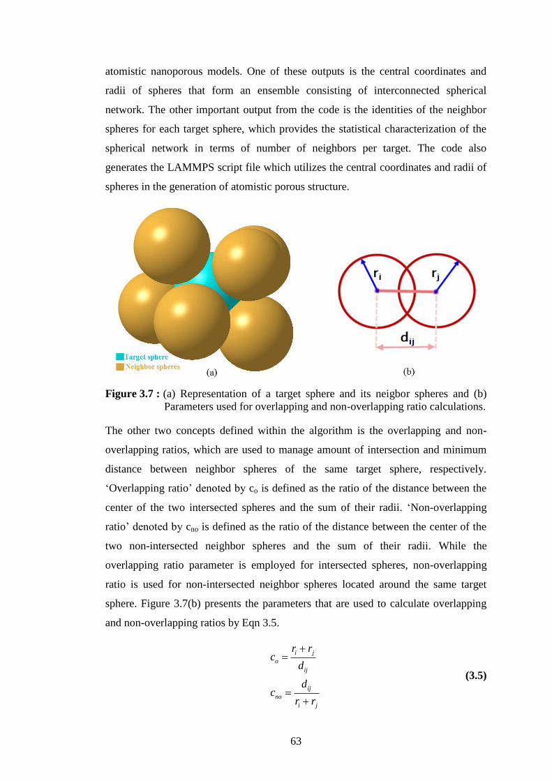
63

atomistic nanoporous models. One of these outputs is the central coordinates and

radii of spheres that form an ensemble consisting of interconnected spherical

network. The other important output from the code is the identities of the neighbor

spheres for each target sphere, which provides the statistical characterization of the

spherical network in terms of number of neighbors per target. The code also

generates the LAMMPS script file which utilizes the central coordinates and radii of

spheres in the generation of atomistic porous structure.

Figure 3.7 : (a) Representation of a target sphere and its neigbor spheres and (b)

Parameters used for overlapping and non-overlapping ratio calculations.

The other two concepts defined within the algorithm is the overlapping and non-

overlapping ratios, which are used to manage amount of intersection and minimum

distance between neighbor spheres of the same target sphere, respectively.

‘Overlapping ratio’ denoted by co is defined as the ratio of the distance between the

center of the two intersected spheres and the sum of their radii. ‘Non-overlapping

ratio’ denoted by cno is defined as the ratio of the distance between the center of the

two non-intersected neighbor spheres and the sum of their radii. While the

overlapping ratio parameter is employed for intersected spheres, non-overlapping

ratio is used for non-intersected neighbor spheres located around the same target

sphere. Figure 3.7(b) presents the parameters that are used to calculate overlapping

and non-overlapping ratios by Eqn 3.5.

i j

o

ij

ij

no

i j

r rc

d

dc

r r

(3.5)

64

In Eqn. 3.5, ir and jr are the radii of spheres which are considered for the

overlapping and non-overlapping ratio calculations, and ijd is the distance between

central coordinates of corresponding spheres.

The algorithm used to generate ensemble of randomly intersected spheres starts with

the creation of a sphere randomly located in the design space and issued as the target

sphere to generate neighbor spheres intersected to the target sphere. After completing

the maximum number of neighbor spheres on the target sphere, a new target sphere is

selected amongst the neighbor spheres and creation of the neighbor spheres

progresses to be located on the new target. As the new spheres intersected with

existing spheres are created, ensemble of spheres grows to larger sizes. When the

required size of the ensemble, which depends on the size of the specimen that will be

tested numerically, is reached, creation of spheres is ended.

The central coordinates of neighbor spheres , ,x y z are calculated by using the

central coordinates of the target spheres 0 0 0, ,x y z in the spherical coordinate

system as shown in Eqn. 3.6.

0

0

0

sin cos

sin sin

cos

x x r

y y r

z z r

(3.6)

In Eqn. 3.6, and are angular components of the spherical coordinates and are

selected randomly from specific ranges. In this regard, is randomly chosen from 0

to π/2 and is randomly chosen from 0 to π. The other parameter r represents the

distance between the target sphere and corresponding neighbor sphere. It is

determined by the overlapping ratio defined as a preliminary for the numerical

model. If the neighbor sphere, which is selected randomly by these stochastic

spherical coordinates, does not satisfy the constraints which are defined by

overlapping and non-overlapping ratios, a new random neighbor sphere is generated

until all the constraints are satisfied.

As mentioned above, central coordinates of neighbor spheres are generated in a

stochastic manner. However, for the purpose of controlling certain properties of the

nanoporous structure such as porosity and ligament size distribution, several design

parameters are maintained to be adjustable in the random sphere generation

65

algorithm: One of these design parameters is the range of diameter values of spheres

that are generated. So, by this way the radii of spheres can be selected randomly from

a pre-defined array in the process of sphere generation. By controlling the size of

spheres, cell sizes in the porous structure can be kept under control.

Figure 3.8 : Generation of a CAD foam model by spherical ensemble approach.

The other parameter that is controlled within the generation process is the maximum

number of neighbor spheres intersected with a target sphere. This parameter affects

the porosity as well as the degree of interconnectivity of the porous structure. Beside

these parameters, overlapping and non-overlapping parameters which have been

defined previously are varied to generate porous structures with different porosities.

In the mean time, some of these are interrelated with each other. For example, as the

overlapping ratio is increased, the number of neighbor spheres per target sphere

should be decreased accordingly due to the reason that the surface area reserved on

the target sphere for one intersection increases. Similarly, as the non-overlapping

ratio is decreased the number of neighbor spheres per one target can be increased.

Because, non-overlapping ratio is a measure of minimum distance between the

neighbor spheres located on the same target; thus, decreasing this distance enables to

place more spheres on the target. For these reasons, while setting these initial

parameters, the inter-relationships between these parameters should also be

considered.

Non-overlapping ratio values are kept above 1 to avoid any possible intersections

between neighbor spheres around the same target sphere. The volume between non-

intersected spheres defines the ligaments and junctions (see Figure 3.9). Therefore,

varying the overlapping ratio enables to alter ligament and junction sizes.

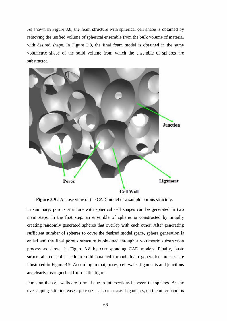
66

As shown in Figure 3.8, the foam structure with spherical cell shape is obtained by

removing the unified volume of spherical ensemble from the bulk volume of material

with desired shape. In Figure 3.8, the final foam model is obtained in the same

volumetric shape of the solid volume from which the ensemble of spheres are

substracted.

Figure 3.9 : A close view of the CAD model of a sample porous structure.

In summary, porous structure with spherical cell shapes can be generated in two

main steps. In the first step, an ensemble of spheres is constructed by initially

creating randomly generated spheres that overlap with each other. After generating

sufficient number of spheres to cover the desired model space, sphere generation is

ended and the final porous structure is obtained through a volumetric substraction

process as shown in Figure 3.8 by corresponding CAD models. Finally, basic

structural items of a cellular solid obtained through foam generation process are

illustrated in Figure 3.9. According to that, pores, cell walls, ligaments and junctions

are clearly distinguished from in the figure.

Pores on the cell walls are formed due to intersections between the spheres. As the

overlapping ratio increases, pore sizes also increase. Ligaments, on the other hand, is

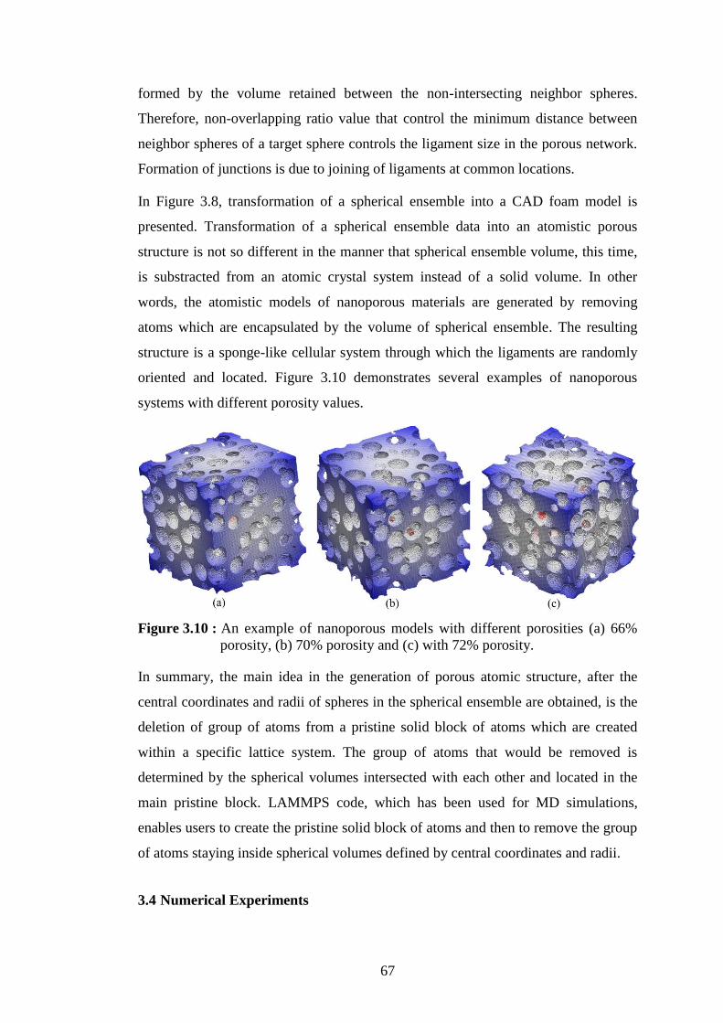
67

formed by the volume retained between the non-intersecting neighbor spheres.

Therefore, non-overlapping ratio value that control the minimum distance between

neighbor spheres of a target sphere controls the ligament size in the porous network.

Formation of junctions is due to joining of ligaments at common locations.

In Figure 3.8, transformation of a spherical ensemble into a CAD foam model is

presented. Transformation of a spherical ensemble data into an atomistic porous

structure is not so different in the manner that spherical ensemble volume, this time,

is substracted from an atomic crystal system instead of a solid volume. In other

words, the atomistic models of nanoporous materials are generated by removing

atoms which are encapsulated by the volume of spherical ensemble. The resulting

structure is a sponge-like cellular system through which the ligaments are randomly

oriented and located. Figure 3.10 demonstrates several examples of nanoporous

systems with different porosity values.

Figure 3.10 : An example of nanoporous models with different porosities (a) 66%

porosity, (b) 70% porosity and (c) with 72% porosity.

In summary, the main idea in the generation of porous atomic structure, after the

central coordinates and radii of spheres in the spherical ensemble are obtained, is the

deletion of group of atoms from a pristine solid block of atoms which are created

within a specific lattice system. The group of atoms that would be removed is

determined by the spherical volumes intersected with each other and located in the

main pristine block. LAMMPS code, which has been used for MD simulations,

enables users to create the pristine solid block of atoms and then to remove the group

of atoms staying inside spherical volumes defined by central coordinates and radii.

3.4 Numerical Experiments

68

By employing nanoporous generation method described in the previous section,

several test specimens with different porosities were generated to investigate the

mechanical behavior of nanoporous structures. In this regard, six different

nanoporous models with porosities 0.66, 0.70, 0.72, 0.75, 0.77 and 0.78 were

generated by varying overlapping ratio parameter which control the amount of

intersection between spheres as explained in the previous section. Parameters that

were employed in the generation process of the nanoporous specimens are given in

Table 3.1 together with the characterization results of the specimens. According to

that, radii of the spheres used in the porous network varies between 2nm and 30nm.

The other important parameter not shown in Table 3.1, non-overlapping ratio, was

kept constant with the value of 1.1 for all specimens. Beside this, the minimum

number of neighbor spheres placed on each target spheres was set to 5 for all

samples.

Figure 3.11 : Sectioning characterization of nanoporous samples at different sections.

Generated nanoporous samples were subjected to characterization by serial

sectioning and measuring the ligament thicknesses on each sections. Resulting from

this characterization study, it was concluded that as the porosity value increases, as

interpreted from Table 3.1, the minimum and maximum ligament sizes through the

network decreases as well.

The most direct way of varying ligament size, defined here as the smallest width of a

ligament, is to vary the range of the overlapping ratio in the algorithm while fixing

other parameters. Note that a porosity of 78% represents the upper limit below which

a nanoporous structure can be generated without any pre-existing broken ligaments

in the structure.

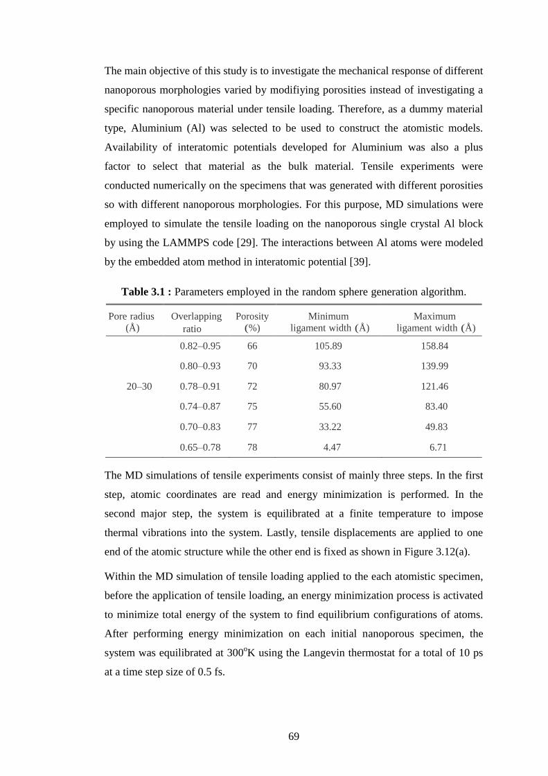
69

The main objective of this study is to investigate the mechanical response of different

nanoporous morphologies varied by modifiying porosities instead of investigating a

specific nanoporous material under tensile loading. Therefore, as a dummy material

type, Aluminium (Al) was selected to be used to construct the atomistic models.

Availability of interatomic potentials developed for Aluminium was also a plus

factor to select that material as the bulk material. Tensile experiments were

conducted numerically on the specimens that was generated with different porosities

so with different nanoporous morphologies. For this purpose, MD simulations were

employed to simulate the tensile loading on the nanoporous single crystal Al block

by using the LAMMPS code [29]. The interactions between Al atoms were modeled

by the embedded atom method in interatomic potential [39].

Parameters employed in the random sphere generation algorithm. Table 3.1 :

Pore radius

(Å)

Overlapping

ratio

Porosity

(%)

Minimum

ligament width (Å)

Maximum

ligament width (Å)

0.82–0.95 66 105.89 158.84

0.80–0.93 70 93.33 139.99

20–30 0.78–0.91 72 80.97 121.46

0.74–0.87 75 55.60 83.40

0.70–0.83 77 33.22 49.83

0.65–0.78 78 4.47 6.71

The MD simulations of tensile experiments consist of mainly three steps. In the first

step, atomic coordinates are read and energy minimization is performed. In the

second major step, the system is equilibrated at a finite temperature to impose

thermal vibrations into the system. Lastly, tensile displacements are applied to one

end of the atomic structure while the other end is fixed as shown in Figure 3.12(a).

Within the MD simulation of tensile loading applied to the each atomistic specimen,

before the application of tensile loading, an energy minimization process is activated

to minimize total energy of the system to find equilibrium configurations of atoms.

After performing energy minimization on each initial nanoporous specimen, the

system was equilibrated at 300oK using the Langevin thermostat for a total of 10 ps

at a time step size of 0.5 fs.

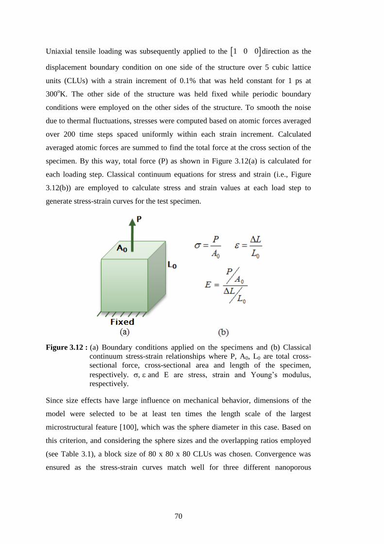
70

Uniaxial tensile loading was subsequently applied to the 1 0 0 direction as the

displacement boundary condition on one side of the structure over 5 cubic lattice

units (CLUs) with a strain increment of 0.1% that was held constant for 1 ps at

300oK. The other side of the structure was held fixed while periodic boundary

conditions were employed on the other sides of the structure. To smooth the noise

due to thermal fluctuations, stresses were computed based on atomic forces averaged

over 200 time steps spaced uniformly within each strain increment. Calculated

averaged atomic forces are summed to find the total force at the cross section of the

specimen. By this way, total force (P) as shown in Figure 3.12(a) is calculated for

each loading step. Classical continuum equations for stress and strain (i.e., Figure

3.12(b)) are employed to calculate stress and strain values at each load step to

generate stress-strain curves for the test specimen.

Figure 3.12 : (a) Boundary conditions applied on the specimens and (b) Classical

continuum stress-strain relationships where P, A0, L0 are total cross-

sectional force, cross-sectional area and length of the specimen,

respectively. and E are stress, strain and Young’s modulus,

respectively.

Since size effects have large influence on mechanical behavior, dimensions of the

model were selected to be at least ten times the length scale of the largest

microstructural feature [100], which was the sphere diameter in this case. Based on

this criterion, and considering the sphere sizes and the overlapping ratios employed

(see Table 3.1), a block size of 80 x 80 x 80 CLUs was chosen. Convergence was

ensured as the stress-strain curves match well for three different nanoporous

71

structures generated randomly with the same parameter values for the largest

overlapping ratios in the algorithm described above.

3.5 Results

As described in the previous section, stress and strain values were calculated by

employing classical continuum equations (see Figure 3.12(b)) at each load step. The

stress-strain curves obtained for the nanoporous specimens with various porosities

under tensile loading are shown in Figure 3.13(a). One of the first observations in

these plots is that the slope of the initial linear portion of stress-strain curve, which is

called as the Young’s modulus, increases as the porosity decreases. Similar behavior

is also observed for the yield and ultimate tensile strength values of test specimens,

which is also consistent with the general mechanical behavior of macroscopic porous

structures [101-103]. Another result that can be interpreted from the stress-strain

curves of nanoporous specimens is that the less-stiff behavior emerges following the

maximum stress point. This softening behavior observed in all the present

simulations after reaching the peak stress is also consistent with previous

experimental results reported on nanoporous -Au [104,105]. In their study Biener et

al. [61], interpreted the softening behavior as “macroscopic brittle but microscopic

ductile behavior,” where the weakest ligament undergoes necking, and its subsequent

rupture overloads the adjacent ligaments, ultimately leading to catastrophic failure of

the nanoporous-Au structure. In order to investigate the softening region of stress-

strain curves, softening rates for each specimen were taken into account

quantitatively. In this regard, softening rates or in other words the postpeak tangent

modulus were determined from the peak stress point of each stress-strain curve in

Figure 3.13(a) and all postpeak tangent modulus values were plotted against the

porosity in Figure 3.13(b).

The most surprising observation from Figure 3.13(b) is that the material softens more

slowly with increasing porosity from 66% to 72%, but softens much more slowly

when porosity reaches to 75% and beyond. This behavior gives a general idea that

structures with porosity less than or equal to 72% fail according to the same

mechanism, while structures with porosity higher than or equal to 75% fail according

to another mechanism. In other words, nanoporous structures with porosities less

than 75% demonstrate a different deformation mechanism than the nanoporous

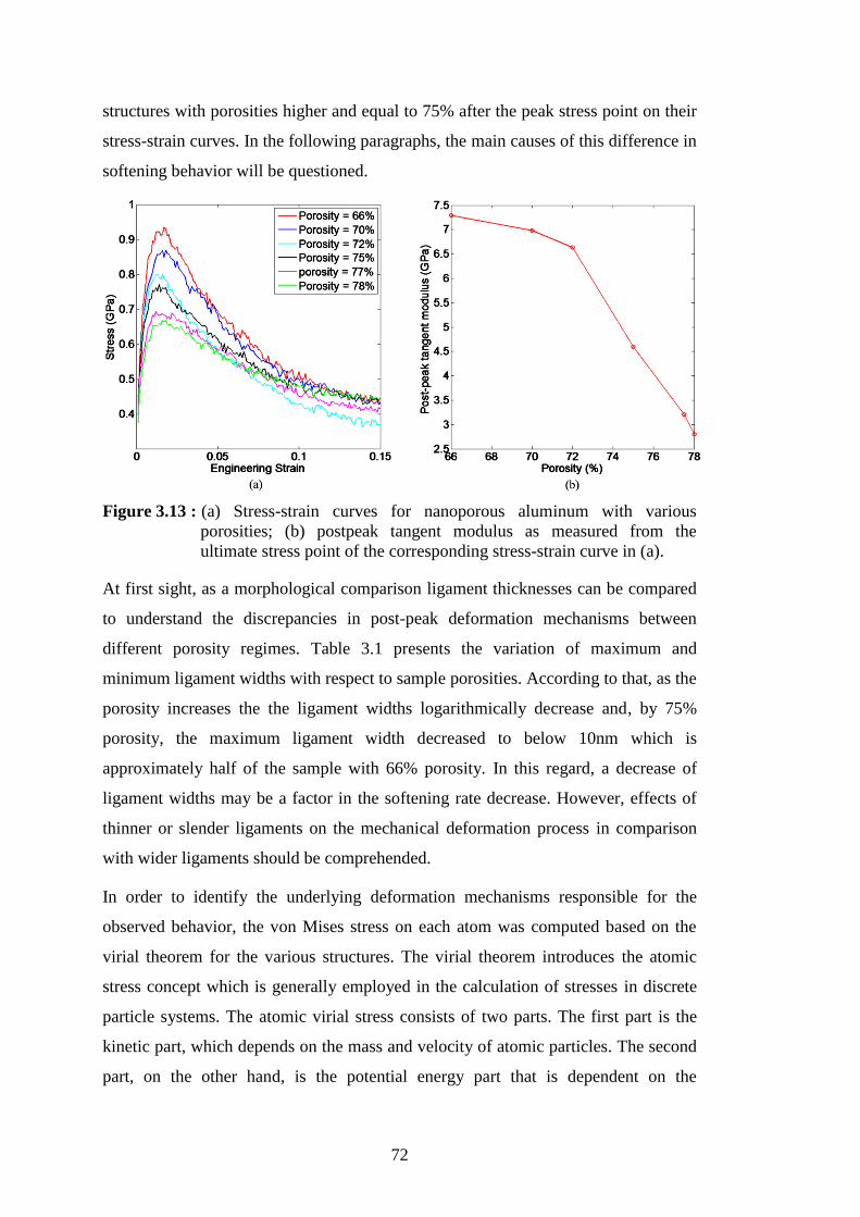
72

structures with porosities higher and equal to 75% after the peak stress point on their

stress-strain curves. In the following paragraphs, the main causes of this difference in

softening behavior will be questioned.

Figure 3.13 : (a) Stress-strain curves for nanoporous aluminum with various

porosities; (b) postpeak tangent modulus as measured from the

ultimate stress point of the corresponding stress-strain curve in (a).

At first sight, as a morphological comparison ligament thicknesses can be compared

to understand the discrepancies in post-peak deformation mechanisms between

different porosity regimes. Table 3.1 presents the variation of maximum and

minimum ligament widths with respect to sample porosities. According to that, as the

porosity increases the the ligament widths logarithmically decrease and, by 75%

porosity, the maximum ligament width decreased to below 10nm which is

approximately half of the sample with 66% porosity. In this regard, a decrease of

ligament widths may be a factor in the softening rate decrease. However, effects of

thinner or slender ligaments on the mechanical deformation process in comparison

with wider ligaments should be comprehended.

In order to identify the underlying deformation mechanisms responsible for the

observed behavior, the von Mises stress on each atom was computed based on the

virial theorem for the various structures. The virial theorem introduces the atomic

stress concept which is generally employed in the calculation of stresses in discrete

particle systems. The atomic virial stress consists of two parts. The first part is the

kinetic part, which depends on the mass and velocity of atomic particles. The second

part, on the other hand, is the potential energy part that is dependent on the

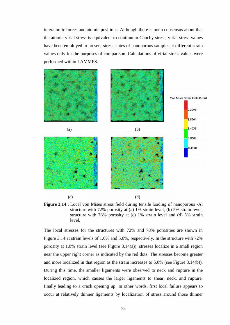
73

interatomic forces and atomic positions. Although there is not a consensus about that

the atomic virial stress is equivalent to continuum Cauchy stress, virial stress values

have been employed to present stress states of nanoporous samples at different strain

values only for the purposes of comparison. Calculations of virial stress values were

performed within LAMMPS.

Figure 3.14 : Local von Mises stress field during tensile loading of nanoporous -Al

structure with 72% porosity at (a) 1% strain level, (b) 5% strain level,

structure with 78% porosity at (c) 1% strain level and (d) 5% strain

level.

The local stresses for the structures with 72% and 78% porosities are shown in

Figure 3.14 at strain levels of 1.0% and 5.0%, respectively. In the structure with 72%

porosity at 1.0% strain level (see Figure 3.14(a)), stresses localize in a small region

near the upper right corner as indicated by the red dots. The stresses become greater

and more localized in that region as the strain increases to 5.0% (see Figure 3.14(b)).

During this time, the smaller ligaments were observed to neck and rupture in the

localized region, which causes the larger ligaments to shear, neck, and rupture,

finally leading to a crack opening up. In other words, first local failure appears to

occur at relatively thinner ligaments by localization of stress around those thinner

74

ligaments. The reason why the number of stress localized regions is less is that the

compliance between the junctions and ligaments are low. Due to low geometrical

compliance between ligaments and junctions, the stress flow through junctions to

other ligaments is limited, which in turn results in highly localized stress regions in a

few areas close to the load application region. Therefore, the stress flow cannot

diffuse into the inner regions away from the load application region.

However, in the structure with 78% porosity, the local stresses distribute in a very

different manner. As shown in Figure 3.14(c) the number of spots with high local

stress, red spots in the figure increases near the upper right corner. As the applied

strain increases further, the number of spots with high local stress continues to

increase away from the upper right corner, while the stresses in these spots also

increase (Figure 3.14(d)). At the strain level of 5.0% where the material has

undergone some softening, some ligaments have already undergone necking and

ruptured at various isolated locations. This behavior can be explained with the

geometric compliance between the ligaments and the junctions in contrast to the case

in lower porosity of 72%. As the porosity increases, the degree of compliance

between ligaments and junctions increases as well. For this reason, the stress flow

through the porous network is more homogenous comparing to the lower porosity

structure. Because junctions and ligaments in 75% porosity structure are more

compatible, the stress flow is not confined to a limited region and diffuses into the

inner regions away from the load application area as shown in Figure 3.14(d) with

more evenly distributed red spot areas. At 5% strain, the spots with high stresses

scatter throughout the structure (see Figure 3.14(d)), while the rupture of ligaments

finally leads to the crack opening in the upper right corner for increased strains.

Because tendency of stress localization is higher for lower porosity nanoporous

structures due to less compliant ligament-junction pairs, the stress values should be

higher than the values in the nanoporous structure with higher porosity. To confirm

this deduction quantitatively, local stress distributions at 5.0% strain, at which the

overall stress is approximately equal for the 72% and 78% nanoporous structures, are

plotted in Figure 3.15 for comparison. The key evidence is that the tail of the stress

distribution of the 72% nanoporous structure is heavier than that of the 78%

structure, and the extreme stress values are almost 2 GPa higher in the 72%

nanoporous structure.

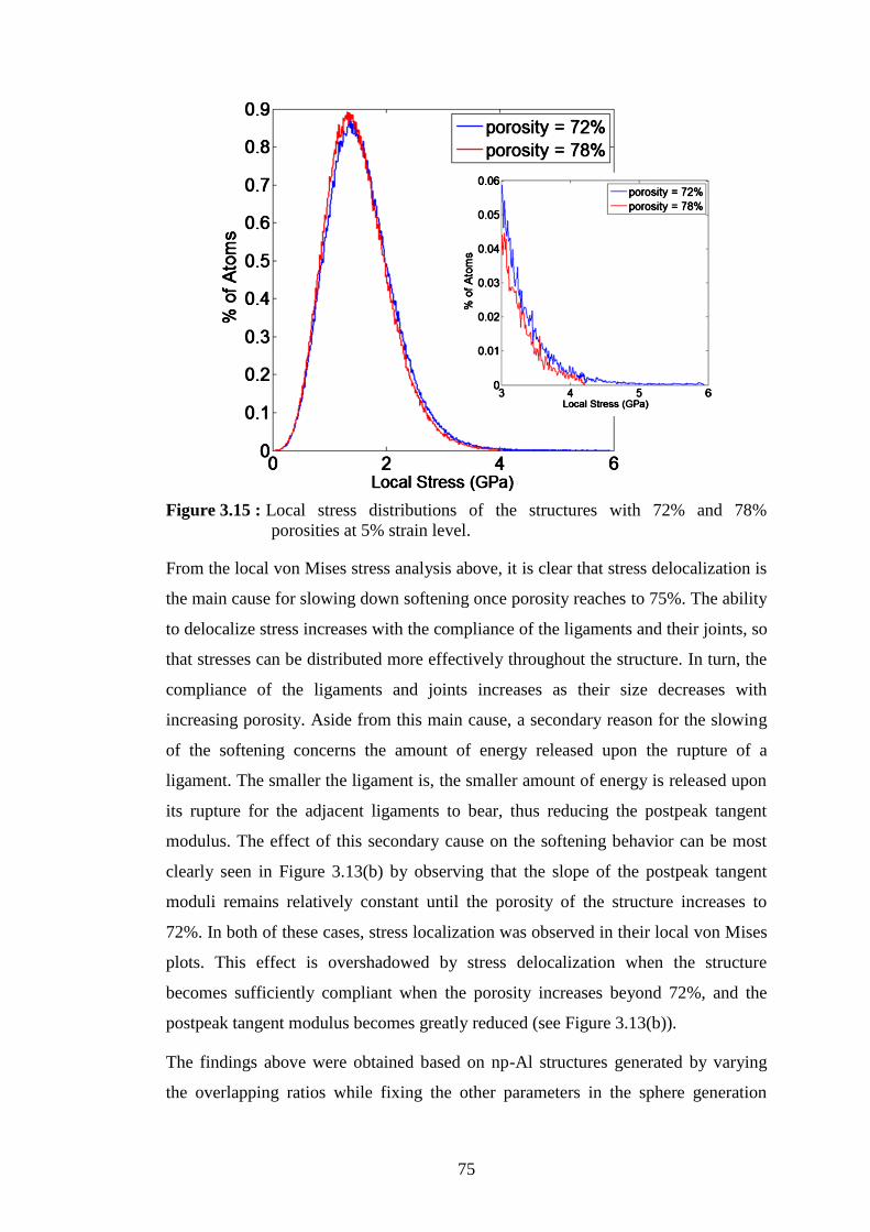
75

Figure 3.15 : Local stress distributions of the structures with 72% and 78%

porosities at 5% strain level.

From the local von Mises stress analysis above, it is clear that stress delocalization is

the main cause for slowing down softening once porosity reaches to 75%. The ability

to delocalize stress increases with the compliance of the ligaments and their joints, so

that stresses can be distributed more effectively throughout the structure. In turn, the

compliance of the ligaments and joints increases as their size decreases with

increasing porosity. Aside from this main cause, a secondary reason for the slowing

of the softening concerns the amount of energy released upon the rupture of a

ligament. The smaller the ligament is, the smaller amount of energy is released upon

its rupture for the adjacent ligaments to bear, thus reducing the postpeak tangent

modulus. The effect of this secondary cause on the softening behavior can be most

clearly seen in Figure 3.13(b) by observing that the slope of the postpeak tangent

moduli remains relatively constant until the porosity of the structure increases to

72%. In both of these cases, stress localization was observed in their local von Mises

plots. This effect is overshadowed by stress delocalization when the structure

becomes sufficiently compliant when the porosity increases beyond 72%, and the

postpeak tangent modulus becomes greatly reduced (see Figure 3.13(b)).

The findings above were obtained based on np-Al structures generated by varying

the overlapping ratios while fixing the other parameters in the sphere generation

76

algorithm (see Appendix). To verify these findings more comprehensively, structures

with different sphere size ranges (20–30, 30–40, and 40–50Å) but almost identical

porosities (within 0.01% porosity difference) were tested by using the MD

simulations. In addition, all these tests were repeated with tensile loading in the

1 1 1 direction to check the influence of crystallographic orientation. The

findings in all these tests were found to be consistent with one another.

3.6 Summary and Conclusion

Nanoporous materials are subset of concentional cellular materials having typically

pore diameters in the range of 1-100nm with the porosity generally higher than 40%.

The most significant property of nanoporous materials is their ultra-high surface

area-to-volume ratios, and combined with their lightweight, they are extraordinary

candidates for applications such as catalyzing, sensing, filtration and adsorbing.

Due to their complex morphology, numerical modeling of their atomistic structure is

the most challenging point for the numerical investigation of their properties.

Because of this issue, a number of numerical studies focusing on the behavior of

nanoporous materials was published in literature. In this regard, one of the

contributions of this chapter is the introduction of an algorithm for the generation of

atomistic models of nanoporous structures.

Nanoporous structures can be considered as the random network of ligaments which

are joined with each other at the junctions. In the algorithm developed for the

generation of random network of ligaments, cell shapes are assumed to be spherical.

The main principle of the proposed algorithm is the creation of an ensemble of

spheres in which the spheres are intersected with each other in a controlled manner.

Radii and central coordinates of spheres within the ensemble are utilized to remove

atoms from a bulk crystalline structure and eventually a porous structure that consists

of randomly intersected ligaments. As a product of overall generation process,

randomly oriented ligaments with non-homogenous mass distribution along their

length are formed and the porosity control on the random network is achieved.

Different nanoporous specimens with different porosity values were generated to

investigate the mechanical behavior of nanoporous materials.

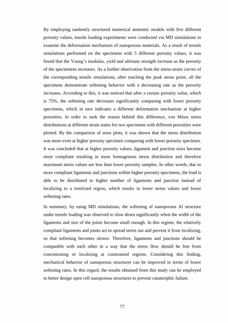
77

By employing randomly structured numerical atomistic models with five different

porosity values, tensile loading experiments were conducted via MD simulations to

examine the deformation mechanism of nanoporous materials. As a result of tensile

simulations performed on the specimens with 5 different porosity values, it was

found that the Young’s modulus, yield and ultimate strength increase as the porosity

of the speciemens increases. As a further observation from the stress-strain curves of

the corresponding tensile simulations, after reaching the peak stress point, all the

specimens demonstrate softening behavior with a decreasing rate as the porosity

increases. According to this, it was noticed that after a certain porosity value, which

is 75%, the softening rate decreases significantly comparing with lower porosity

specimens, which in turn indicates a different deformation mechanism at higher

porosities. In order to seek the reason behind this difference, von Mises stress

distributions at different strain states for two specimens with different porosities were

plotted. By the comparison of sress plots, it was shown that the stress distribution

was more even at higher porosity specimen comparing with lower porosity specimen.

It was concluded that at higher porosity values, ligament and junction sizes become

more compliant resulting in more homogenous stress distribution and therefore

maximum stress values are less than lower porosity samples. In other words, due to

more compliant ligaments and junctions within higher porosity specimens, the load is

able to be distributed to higher number of ligaments and junction instead of

localizing to a restricted region, which results in lower stress values and lower

softening rates.

In summary, by using MD simulations, the softening of nanoporous Al structure

under tensile loading was observed to slow down significantly when the width of the

ligaments and size of the joints become small enough. In this regime, the relatively

compliant ligaments and joints act to spread stress out and prevent it from localizing,

so that softening becomes slower. Therefore, ligaments and junctions should be

compatible with each other in a way that the stress flow should be free from

concentrating or localizing at constrained regions. Considering this finding,

mechanical behavior of nanoporous structures can be improved in terms of lower

softening rates. In this regard, the results obtained from this study can be employed

to better design open cell nanoporous structures to prevent catastrophic failure.

79

4. STOCHASTIC MODELING AND MECHANICS OF CARBON

NANOTUBE NETWORKS

4.1 Purpose

Carbon nanotubes (CNTs) are one of the presents of nanotechnology being

investigated due to their extraordinary mechanical, thermal and electrical properties.

Carbon nanotube networks feed the idea that the CNTs can be used as the building

blocks of new advanced materials utilizing the superior characteristics of CNTs. In

this way, nanoscale features of the CNTs can be scaled up to even continuum

proportions. In the first stage of this study, 2-D and 3-D CNT network generation

methods were introduced by which the geometrical parameters, such as CNT length,

chirality, intersection angle and junctional density, can be controlled and a random

CNT network is obtained. Then, MD simulations were used to create covalent bonds

between the intersecting CNTs, which allow the investigation of the mechanical,

thermal and electrical properties of random CNT networks. In the second stage of the

study, tensile and shear loading experiments performed on the atomistic models of

CNT networks were conducted by the MD simulations to investigate mechanical

behavior of 3-D CNT networks that consist of covalently bonded CNTs.

4.2 Literature Review

Carbon nanotubes (CNTs) are one of the extraordinary nanomaterials that are

promising candidates for thermal, electrical and structural applications due to their

unique properties [106]. Since their discovery by Iijima (1991), thousands of studies,

so far, have been adopted to their exceptional high strength and unusual electrical

and thermal properties, displaying the desirable nature of their multifunctional

capability. Due to combination of remarkable mechanical, thermal and electrical

properties of CNTs, they have potential applications in different fields such as

material reinforcement, field emission panel display, chemical sensing, drug delivery

and nanoelectronics. On the other hand, there are already development studies by

NASA for the usage of the CNTs at space applications where lightweight materials

80

with high strength/stiffness-to-weight ratio are very important to design cost

effective structures. In this regard, composite materials reinforced by the CNTs

represent higher strength-to-weight ratios than any other presently known materials

[107]. Beside that, several companies, Samsung and NEC among others, that are

known as electronic device manufacturers have already employed the CNTs in field

emission displays [4] resulting in remarkable quality increase in their products and

are determined to continue to the investments in this field. Meanwhile, due to their

high compatibility to biological medium and their high strength, the CNTs are also

exceptional candidates for biomedical applications. For example, conventional

composite materials such as fiber-based composites have shown to be inadequate in

the replacement of bone and teeth due to insufficient mechanical properties and most

importantly due to interfacial instability in biologic conditions causing degradation

of the materials. However, it is well known that carbon based materials shows high

resistivity against degradation in chemical environments that exist in the body. In this

regard, CNT based artificial muscle [6] recently developed is one of the steps

towards biomedical applications of the CNTs that offers superiorities over

conventional technologies. Moreover, the CNTs can also be employed as drug

delivery devices because they could be integrated into the biological tissue locations

where the drug delivery would be carried out without any tissue damaged.

Experimental studies on the determination of the Young’s modulus of Table 4.1 :

CNTs.

Author (s) Modulus

(TPa)

Deviation

(TPa) Test Method Type

Treacy et al. [108] 1.8 1.4 Thermal vibrations MWNT

Wong et al. [109] 1.28 0.6 Cantilever bending MWNT

Krishnan et al. [110] 1.3 0.5 Thermal vibrations MWNT

Salvetat et al. [111] 0.81 0.41 3 point bending Bundles

Salvetat et al. [111] 1.28 0.59 3 point bending MWNT

Tombler et al. [112] 1.2 - 3 point bending SWNT

Cooper & Young [113] 0.78-2.34 - Raman spectroscopy SWNT

Yu et al. [114] 0.27-0.95 - Tension MWNT

Lourie & Wagner [115] 2.8-3.6 - Raman spectroscopy SWNT

Lourie & Wagner [115] 1.7-2.4 - Raman spectroscopy MWNT

Yu et al. [114] 0.32-1.47 - Tension Ropes

In the applications where mechanical characteristics of the CNTs play decisive role

in the functionality of nanodevices or nanostructures, it is vital to understand the

mechanical properties of CNTs. In this regard, there are numerous studies in

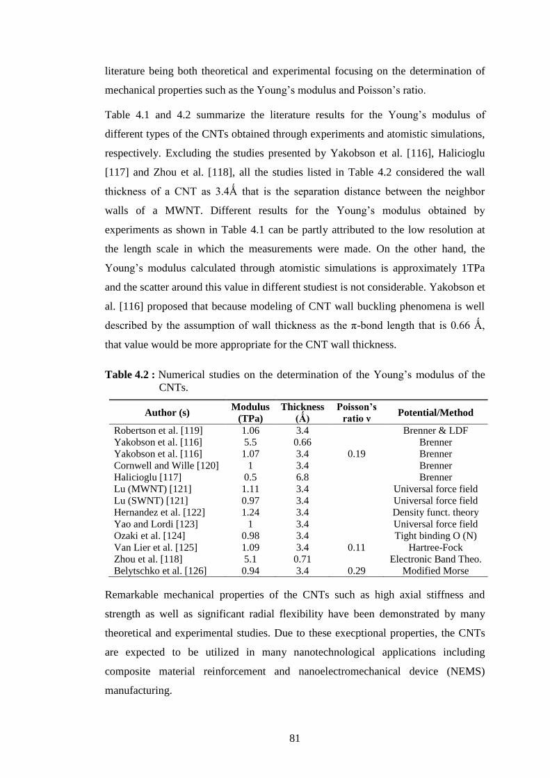
81

literature being both theoretical and experimental focusing on the determination of

mechanical properties such as the Young’s modulus and Poisson’s ratio.

Table 4.1 and 4.2 summarize the literature results for the Young’s modulus of

different types of the CNTs obtained through experiments and atomistic simulations,

respectively. Excluding the studies presented by Yakobson et al. [116], Halicioglu

[117] and Zhou et al. [118], all the studies listed in Table 4.2 considered the wall

thickness of a CNT as 3.4Ǻ that is the separation distance between the neighbor

walls of a MWNT. Different results for the Young’s modulus obtained by

experiments as shown in Table 4.1 can be partly attributed to the low resolution at

the length scale in which the measurements were made. On the other hand, the

Young’s modulus calculated through atomistic simulations is approximately 1TPa

and the scatter around this value in different studiest is not considerable. Yakobson et

al. [116] proposed that because modeling of CNT wall buckling phenomena is well

described by the assumption of wall thickness as the π-bond length that is 0.66 Ǻ,

that value would be more appropriate for the CNT wall thickness.

Numerical studies on the determination of the Young’s modulus of the Table 4.2 :

CNTs.

Author (s) Modulus

(TPa)

Thickness

(Ǻ)

Poisson’s

ratio ν Potential/Method

Robertson et al. [119] 1.06 3.4 Brenner & LDF

Yakobson et al. [116] 5.5 0.66 Brenner

Yakobson et al. [116] 1.07 3.4 0.19 Brenner

Cornwell and Wille [120] 1 3.4 Brenner

Halicioglu [117] 0.5 6.8 Brenner

Lu (MWNT) [121] 1.11 3.4 Universal force field

Lu (SWNT) [121] 0.97 3.4 Universal force field

Hernandez et al. [122] 1.24 3.4 Density funct. theory

Yao and Lordi [123] 1 3.4 Universal force field

Ozaki et al. [124] 0.98 3.4 Tight binding O (N)

Van Lier et al. [125] 1.09 3.4 0.11 Hartree-Fock

Zhou et al. [118] 5.1 0.71 Electronic Band Theo.

Belytschko et al. [126] 0.94 3.4 0.29 Modified Morse

Remarkable mechanical properties of the CNTs such as high axial stiffness and

strength as well as significant radial flexibility have been demonstrated by many

theoretical and experimental studies. Due to these execptional properties, the CNTs

are expected to be utilized in many nanotechnological applications including

composite material reinforcement and nanoelectromechanical device (NEMS)

manufacturing.

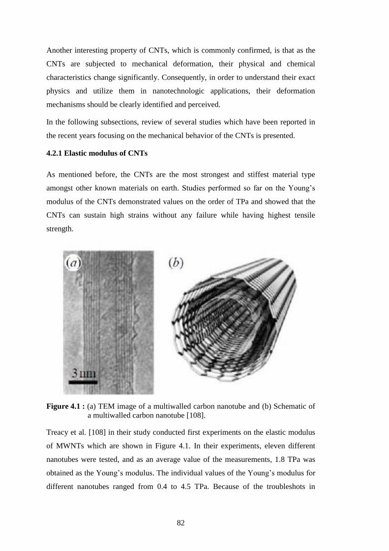
82

Another interesting property of CNTs, which is commonly confirmed, is that as the

CNTs are subjected to mechanical deformation, their physical and chemical

characteristics change significantly. Consequently, in order to understand their exact

physics and utilize them in nanotechnologic applications, their deformation

mechanisms should be clearly identified and perceived.

In the following subsections, review of several studies which have been reported in

the recent years focusing on the mechanical behavior of the CNTs is presented.

4.2.1 Elastic modulus of CNTs

As mentioned before, the CNTs are the most strongest and stiffest material type

amongst other known materials on earth. Studies performed so far on the Young’s

modulus of the CNTs demonstrated values on the order of TPa and showed that the

CNTs can sustain high strains without any failure while having highest tensile

strength.

Figure 4.1 : (a) TEM image of a multiwalled carbon nanotube and (b) Schematic of

a multiwalled carbon nanotube [108].

Treacy et al. [108] in their study conducted first experiments on the elastic modulus

of MWNTs which are shown in Figure 4.1. In their experiments, eleven different

nanotubes were tested, and as an average value of the measurements, 1.8 TPa was

obtained as the Young’s modulus. The individual values of the Young’s modulus for

different nanotubes ranged from 0.4 to 4.5 TPa. Because of the troubleshots in

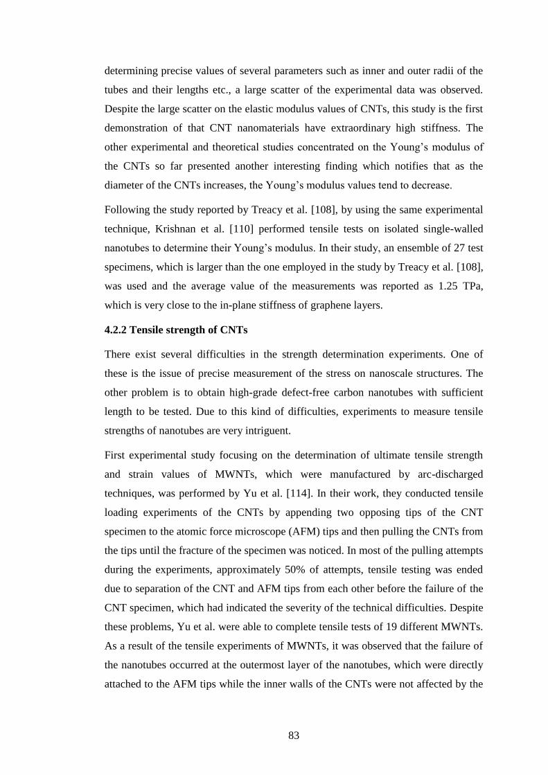
83

determining precise values of several parameters such as inner and outer radii of the

tubes and their lengths etc., a large scatter of the experimental data was observed.

Despite the large scatter on the elastic modulus values of CNTs, this study is the first

demonstration of that CNT nanomaterials have extraordinary high stiffness. The

other experimental and theoretical studies concentrated on the Young’s modulus of

the CNTs so far presented another interesting finding which notifies that as the

diameter of the CNTs increases, the Young’s modulus values tend to decrease.

Following the study reported by Treacy et al. [108], by using the same experimental

technique, Krishnan et al. [110] performed tensile tests on isolated single-walled

nanotubes to determine their Young’s modulus. In their study, an ensemble of 27 test

specimens, which is larger than the one employed in the study by Treacy et al. [108],

was used and the average value of the measurements was reported as 1.25 TPa,

which is very close to the in-plane stiffness of graphene layers.

4.2.2 Tensile strength of CNTs

There exist several difficulties in the strength determination experiments. One of

these is the issue of precise measurement of the stress on nanoscale structures. The

other problem is to obtain high-grade defect-free carbon nanotubes with sufficient

length to be tested. Due to this kind of difficulties, experiments to measure tensile

strengths of nanotubes are very intriguent.

First experimental study focusing on the determination of ultimate tensile strength

and strain values of MWNTs, which were manufactured by arc-discharged

techniques, was performed by Yu et al. [114]. In their work, they conducted tensile

loading experiments of the CNTs by appending two opposing tips of the CNT

specimen to the atomic force microscope (AFM) tips and then pulling the CNTs from

the tips until the fracture of the specimen was noticed. In most of the pulling attempts

during the experiments, approximately 50% of attempts, tensile testing was ended

due to separation of the CNT and AFM tips from each other before the failure of the

CNT specimen, which had indicated the severity of the technical difficulties. Despite

these problems, Yu et al. were able to complete tensile tests of 19 different MWNTs.

As a result of the tensile experiments of MWNTs, it was observed that the failure of

the nanotubes occurred at the outermost layer of the nanotubes, which were directly

attached to the AFM tips while the inner walls of the CNTs were not affected by the

84

tensile loading and came out of the outer wall after the failure of the outer wall as if a

sword was pulled from its sheath. Therefore, this kind of failure was named as

sword-in-sheath mechanism. The ultimate tensile strength and strain values were

reported to be varied in the range from 11 to 63 GPa and between 3 and 12%,

respectively. The large scatter in the experimental data was attributed to the

differences in the content and the number of structural defects in the outermost layers

of MWNT specimens.

Tensile experiments on carbon nanotubes have shown that their tensile failure occurs

at strain value of approximately 15% at room temperature. However, in practice

where structural defects exist on the CNT structure, failure strain values decrease to

6%. In contrast to these values at room temperature, at higher temperatures above

2000oK, ultimate tensile strain values of the SWNTs go up to the strain values of

280%, which can be called as superplastic deformation or super-elongation. This

ductile characteristic can also be noticed at double and triple-walled carbon

nanotubes by the strain values of 190%. Hence, even though carbon nanotubes are

brittle at room temperature, at high temperatures they represent super ductile

characteristics.

Figure 4.2 : Visualization of tensile loading of a single-walled carbon nanotube by

TEM (a-d) Tensile deformation of a SWNT at high temperature. Kinks

are showed by arrowheads. (e-g) Tensile loading of a SWNT with initial

length of 75nm (e) at room temperature, (f) length after elongation, (g)

length at the failure which is 84nm [127].

In their study Huang et al. [127], presented a confirmation of such a remarkable

ductile behavior as shown in Figure 4.2 (a-d). As a result of their tensile experiment,

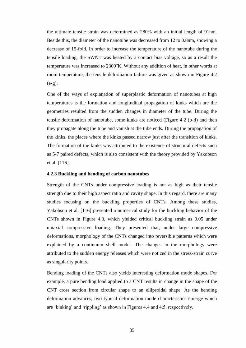
85

the ultimate tensile strain was determined as 280% with an initial length of 91nm.

Beside this, the diameter of the nanotube was decreased from 12 to 0.8nm, showing a

decrease of 15-fold. In order to increase the temperature of the nanotube during the

tensile loading, the SWNT was heated by a contact bias voltage, so as a result the

temperature was increased to 2300oK. Without any addition of heat, in other words at

room temperature, the tensile deformation failure was given as shown in Figure 4.2

(e-g).

One of the ways of explanation of superplastic deformation of nanotubes at high

temperatures is the formation and longitudinal propagation of kinks which are the

geometries resulted from the sudden changes in diameter of the tube. During the

tensile deformation of nanotube, some kinks are noticed (Figure 4.2 (b-d) and then

they propagate along the tube and vanish at the tube ends. During the propagation of

the kinks, the places where the kinks passed narrow just after the transition of kinks.

The formation of the kinks was attributed to the existence of structural defects such

as 5-7 paired defects, which is also consistent with the theory provided by Yakobson

et al. [116].

4.2.3 Buckling and bending of carbon nanotubes

Strength of the CNTs under compressive loading is not as high as their tensile

strength due to their high aspect ratio and cavity shape. In this regard, there are many

studies focusing on the buckling properties of CNTs. Among these studies,

Yakobson et al. [116] presented a numerical study for the buckling behavior of the

CNTs shown in Figure 4.3, which yielded critical buckling strain as 0.05 under

uniaxial compressive loading. They presented that, under large compressive

deformations, morphology of the CNTs changed into reversible patterns which were

explained by a continuum shell model. The changes in the morphology were

attributed to the sudden energy releases which were noticed in the stress-strain curve

as singularity points.

Bending loading of the CNTs also yields interesting deformation mode shapes. For

example, a pure bending load applied to a CNT results in change in the shape of the

CNT cross section from circular shape to an ellipsoidal shape. As the bending

deformation advances, two typical deformation mode characteristics emerge which

are ‘kinking’ and ‘rippling’ as shown in Figures 4.4 and 4.5, respectively.

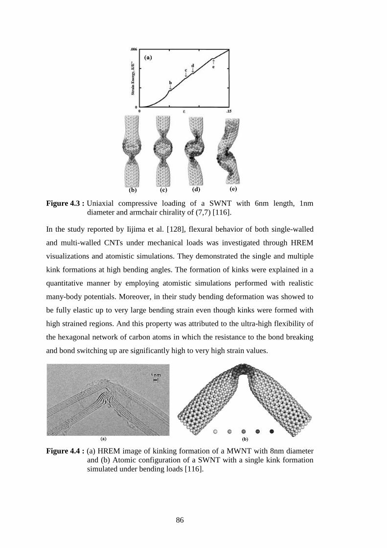
86

Figure 4.3 : Uniaxial compressive loading of a SWNT with 6nm length, 1nm

diameter and armchair chirality of (7,7) [116].

In the study reported by Iijima et al. [128], flexural behavior of both single-walled

and multi-walled CNTs under mechanical loads was investigated through HREM

visualizations and atomistic simulations. They demonstrated the single and multiple

kink formations at high bending angles. The formation of kinks were explained in a

quantitative manner by employing atomistic simulations performed with realistic

many-body potentials. Moreover, in their study bending deformation was showed to

be fully elastic up to very large bending strain even though kinks were formed with

high strained regions. And this property was attributed to the ultra-high flexibility of

the hexagonal network of carbon atoms in which the resistance to the bond breaking

and bond switching up are significantly high to very high strain values.

Figure 4.4 : (a) HREM image of kinking formation of a MWNT with 8nm diameter

and (b) Atomic configuration of a SWNT with a single kink formation

simulated under bending loads [116].

87

Arias and Arroyo [129], in their study, described the nonlinear elastic behavior of

multi-walled CNTs in bending deformation as well as torsional deformation and

built-up a power-law relationship to describe distinct deformation regimes including

the complicated rippling mechanics.

Figure 4.5 : Bending of multi-walled CNTs exhibiting rippling modes of

deformation [129].

4.2.4 Studies on CNT Network Materials

In the recent years, the usefulness of the CNTs has been enormously extended by

their use as CNT networks through which the CNTs are self-intersected in two or

three-dimensional space [130]. Because of their strong electrical conductivity with

high light transmittance, CNT networks are attractive alternatives to silicon based

macroelectronic devices [131]. Initial studies on 2-D CNT networks deposited onto

flexible and polymeric substrates have focused on their electronic and sensor

properties [132-133]. Several CNT network based thin films have been proposed to

obtain lightweight, unbreakable displays and other flexible electronic devices [134].

Bottom-up controlled production of such networks can also enable them to be used in

applications such as sensors, filters, composites and electromechanical actuators

[135]. However, CNT networks also display the charming mechanical abilities of

individual CNTs to macro-mechanical applications such as nanocomposites, similar

to CNTs that are used as reinforcing units in nanocomposites, CNT networks can

88

also be employed in nanocomposites for both reinforcement and damage detection

purposes [136]. In this study, a self-controlled algorithm for generating a 2- or 3-D

CNT network consisting of randomly oriented and intersected CNTs is introduced,

and a heat welding method is applied to sample networks to obtain covalently

bonded networks by MD simulations.

Figure 4.6 : Images of CNT aerogels: (a) Macroscopic pieces of 7.5 mg mL-1 CNT

aerogels, (b) Three polyvinyl alcohol (PVA) reinforced aerogel pillars

supporting 100g, (c) SEM image of open porous structure of aerogel

and (d) TEM image of CNT aerogel [137].

Furthermore, a recently developed CNT aerogel [137] (see Figure 4.6) material that

is nanostructured by self-intersecting CNTs forming a random network at the

continuum scale is one of the important examples displaying an ultra-high stiffness-

to-weight ratio material with conductive properties. Instead of having a

reinforcement role in nanocomposites, this material enables the CNT network to

constitute a bulk material on its own.

Aerogel materials are generally manufactured by applying critical-point-drying

(CPD) or freeze-drying methods on the wet-gel precursors to get rid of liquid content

89

without destroying the interconnected network structure. Aerogel materials have a

cellular structure with very high porosity and ultra-low density. Due to their

microstructural characteristics such as being composed of a flimsy network of

ensemble nanoparticles, they have very high strength-to-weight and surface-area-to-

volume ratios. So far most of the aerogels are manufactured from silica [137] or

pyrolized organic polymers [137]. Silica aerogels are especially attractive due to

their potential applications as ultralight structures, radiation detectors and thermal

insulators. Polymer aerogels have potential usage areas such as battery electrodes

and supercapacitors [138]. In their study, Bryning et al. presented a new class of

aerogels, named as CNT aerogels that consist of percolating networks of CNTs

[137]. They demonstrated that an ensemble of CNTs with small diameters including

single and a few walled CNTs can be used as a precursor to obtain CNT aerogels

which are electrically conductive. Individually CNTs are highly stiff [123] and

effectively electrically conducting nanostructures. Therefore, an ensemble of CNTs

forms an attractive precursor for the generation of aerogels. As shown in Figure

4.6(b), 3 pieces of polyvinyl alcohol (PVA) reinforced CNT aerogel pillars with total

mass of 13mg can support 100g weight which is 8000 times their weight.

Unquestionably, the electrical, thermal or mechanical properties of CNT networks

depend on the density of junctions between the CNTs as well as junction properties

and impurities throughout the network. It has been shown that electrical conductance

and mechanical strength of the junctions may be enhanced by manipulating the

junction area, i.e., by increasing the crossing area [139]. In this manner, the

algorithm proposed in this study will provide complete control on the junction

properties and all the other geometrical features (e.g., CNT length, diameter and

CNT intersection angle), which will enable the exploration of CNT networks

theoretically or numerically by using much more realistic models.

Generally, CNT networks can be formed randomly by depositing the CNTs locally

on the catalyzed substrates by CVD or depositing from CNT embedded polymeric

suspensions remotely by using spin coating, spray coating, or vacuum filtration

techniques [125-127]. With deposition on the catalyzed substrates, alignment of long

CNTs can be more evenly created with directional control, but growth temperatures

are high and unwanted byproducts may also be accumulated [128]. Therefore,

deposition from solutions with suspended CNTs is much more popular due to the

90

ability to produce them at ambient conditions, despite the time-consuming steps such

as purification and dispersion of CNTs.

Most studies investigating the properties of CNT networks are carried out

experimentally following a corresponding production phase. For instance, the

thermal stability of CNT networks produced by the dielectrophoresis method on

microelectrodes is studied experimentally to predict their uses in electrical

applications [140]. Similarly, Wang et al [130] investigated the electrical and

mechanical properties of CNT networks with measurements taken in situ inside the

TEM. In another experimental study, CNT networks are used as reinforcing materials

in composites and compared with composites reinforced by dispersed CNTs [141].

Thostenson and Chou studied the damage and strain-sensing capabilities of CNT

networks utilized in glass fiber-epoxy composites and have shown through tensile

testing that conductive percolating CNT networks can detect the initiation and

progression of damage [142]. Several other studies [143-145] exist in literature on

the electrical, thermal or mechanical properties of CNT networks carrying out

experimental investigations, which, as the other aforementioned studies, inherently

require equipment of manufacturing and testing. On the other hand, the majority of

computational studies focused on the investigation of individual CNTs and their

nanocomposites [146-149]. Due to the lack of a proper method for the generation of

random CNT networks and computational limitations, there is a limited number of

studies that use numerical models and computational methods for the investigations

of CNT networks. Moreover, existing studies [147] that employ numerical network

models mostly use ordered networks which do not include the geometrical

irregularities and other possible imperfections, such as bond re-arrangements, at

junctions. Furthermore, in these models, only one type of junctions are modeled. A

recently published study [150] investigates the mechanical behavior of short single-

walled CNT ( SWNT) aggregates composed of randomly dispersed non-intersected

CNTs by molecular mechanics.

In the first stage of this section, a quasi-random self-intersected CNT network

generation algorithm that enables the control of behavior decisive parameters, such

as the CNT length scale, density of junctions and relative angular position, is

presented and several example networks with different parameters mentioned above

are generated. Following the generation of a CNT network in which the CNT units

91

are so close together that heating to certain temperatures can yield a covalently

bonded network, the MD simulations are carried out to obtain bonded networks. As a

result, parameter-controlled covalently bonded CNT network models can be further

used within the MD simulations to investigate mechanical, thermal and electrical

properties of CNT networks and their co-operating systems (i.e., nanocomposites).

In the second stage, numerical atomistic models, which were generated by the

method introduced in the first stage, have been employed in the MD simulations to

look into the mechanical characteristics of CNT networks under tensile loading. In

order to examine the effect of cross-link density per CNT on the mechanical

response, different CNT network models with different cross-link densities have

been prepared and used in the tensile loading simulations.

4.3 Atomistic Modelling of Heat Welded CNT Networks

Carbon nanotube network materials such as CNT aerogels consist of carbon

nanotubes randomly oriented and physically interrelated with other CNTs existing in

the network. Orientations and interrelations of CNTs in these materials are randomly

organized. Therefore, a stochastic algorithm is required to generate representative

numerical models. In this chapter, general principles and main steps of such a

stochastic algorithm developed within the scope of this study is given. In order to

show the applicability of the proposed method, several examples of numerical

atomistic models have been demonstrated. Moreover, numerical atomistic models

have also been characterized statistically to validate that controlled design

parameters are reflected into the models correctly.

4.3.1 General Concepts

The process of generating random networks can be introduced as a process of

configuring the network items (in this case, randomly intersected CNTs) randomly in

the design space. The placing of network items is carried out under constraints in a

random nature. The algorithm explained here is also employed for the generation of

random porous networks with spherical cells which is used to model microcellular

carbon foams [62].

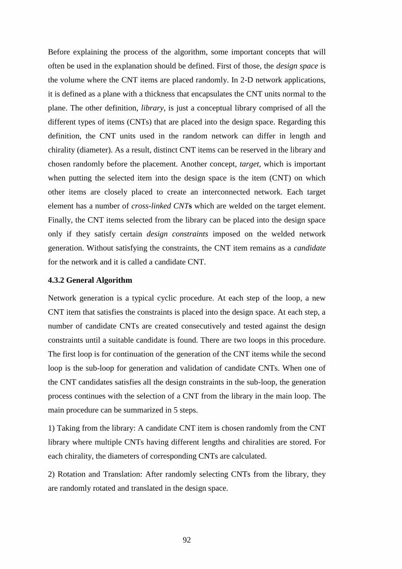
92

Before explaining the process of the algorithm, some important concepts that will

often be used in the explanation should be defined. First of those, the design space is

the volume where the CNT items are placed randomly. In 2-D network applications,

it is defined as a plane with a thickness that encapsulates the CNT units normal to the

plane. The other definition, library, is just a conceptual library comprised of all the

different types of items (CNTs) that are placed into the design space. Regarding this

definition, the CNT units used in the random network can differ in length and

chirality (diameter). As a result, distinct CNT items can be reserved in the library and

chosen randomly before the placement. Another concept, target, which is important

when putting the selected item into the design space is the item (CNT) on which

other items are closely placed to create an interconnected network. Each target

element has a number of cross-linked CNTs which are welded on the target element.

Finally, the CNT items selected from the library can be placed into the design space

only if they satisfy certain design constraints imposed on the welded network

generation. Without satisfying the constraints, the CNT item remains as a candidate

for the network and it is called a candidate CNT.

4.3.2 General Algorithm

Network generation is a typical cyclic procedure. At each step of the loop, a new

CNT item that satisfies the constraints is placed into the design space. At each step, a

number of candidate CNTs are created consecutively and tested against the design

constraints until a suitable candidate is found. There are two loops in this procedure.

The first loop is for continuation of the generation of the CNT items while the second

loop is the sub-loop for generation and validation of candidate CNTs. When one of

the CNT candidates satisfies all the design constraints in the sub-loop, the generation

process continues with the selection of a CNT from the library in the main loop. The

main procedure can be summarized in 5 steps.

1) Taking from the library: A candidate CNT item is chosen randomly from the CNT

library where multiple CNTs having different lengths and chiralities are stored. For

each chirality, the diameters of corresponding CNTs are calculated.

2) Rotation and Translation: After randomly selecting CNTs from the library, they

are randomly rotated and translated in the design space.

93

3) Checking Constraints: After rotation and translation, the design constraints are

checked on the candidate CNT.

4) Making a decision: If the constrains are satisfied, the candidate CNT is placed into

the design space. Otherwise, the procedure is restarted from the beginning.

5) Writing the LAMMPS input data file: Atomic coordinates of each CNT item are

written into different files instead of storing them in the memory. Using these files

(atomic coordinates), the LAMMPS input data file is written to another file.

4.3.2.1 Line segment representation of CNTs

To save computational time, CNTs are represented by 3-D line segments passing

through the central points of the CNTs’ cylindrical geometry as shown in Figure 4.7.

Figure 4.7 : (a) Line segment representation of CNT, (b) Minimum distance between

CNTs by using line segment representation.

Each line segment is represented by the coordinates of end points, which are the

central points of the circles at the CNTs’ end. During the generation process, end

point coordinates are also stored and written to a file. Rotation and translation

operations are also applied to end points, while all distance and angle calculations are

done via the line segments instead of atomic coordinates.

94

The random points on the line segments are generated via parametric line equations

as shown in Eqn.(4.1) where {x0, y0, z0} and {x1, y1, z1} are the tip coordinates and

is the parameter varying in range [0,1] that describes the line segment between the tip

coordinates.

x = x0 + t ( x1 -x0 )

y = y0 + t ( y1 -y0 ) (4.1)

z = z0 + t ( z1 -z0 )

Figure 4.8 : Segmentations of line segments by dividing the segment domain by the

number of cross-links which is four in this example.

The line segment parameter t is also used for the further segmentation of line

segments to position the candidate CNTs on the target CNT more evenly as

represented in Figure 4.8. For instance, a constraint of n cross-links on each target

CNT is maintained by dividing the interval of t by n. Thus, the kth

cross-link is

positioned on the target in the interval of [(k-1)/n, k/n].

4.3.2.2 Target based approach

After putting the first CNT into the design space, it is assigned as the target on which

a certain number of other CNTs should be placed so as to create an interconnected

network. As a result, the CNT item that is assigned as the target will host cross-

linked CNTs. All subsequent CNTs created after the target assignment should be

cross-linked with the target until the number of cross-links reaches the maximum

value, which is predefined as a parameter. After the placement of all cross-linked

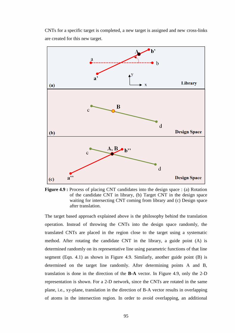
95

CNTs for a specific target is completed, a new target is assigned and new cross-links

are created for this new target.

Figure 4.9 : Process of placing CNT candidates into the design space : (a) Rotation

of the candidate CNT in library, (b) Target CNT in the design space

waiting for intersecting CNT coming from library and (c) Design space

after translation.

The target based approach explained above is the philosophy behind the translation

operation. Instead of throwing the CNTs into the design space randomly, the

translated CNTs are placed in the region close to the target using a systematic

method. After rotating the candidate CNT in the library, a guide point (A) is

determined randomly on its representative line using parametric functions of that line

segment (Eqn. 4.1) as shown in Figure 4.9. Similarly, another guide point (B) is

determined on the target line randomly. After determining points A and B,

translation is done in the direction of the B-A vector. In Figure 4.9, only the 2-D

representation is shown. For a 2-D network, since the CNTs are rotated in the same

plane, i.e., xy-plane, translation in the direction of B-A vector results in overlapping

of atoms in the intersection region. In order to avoid overlapping, an additional

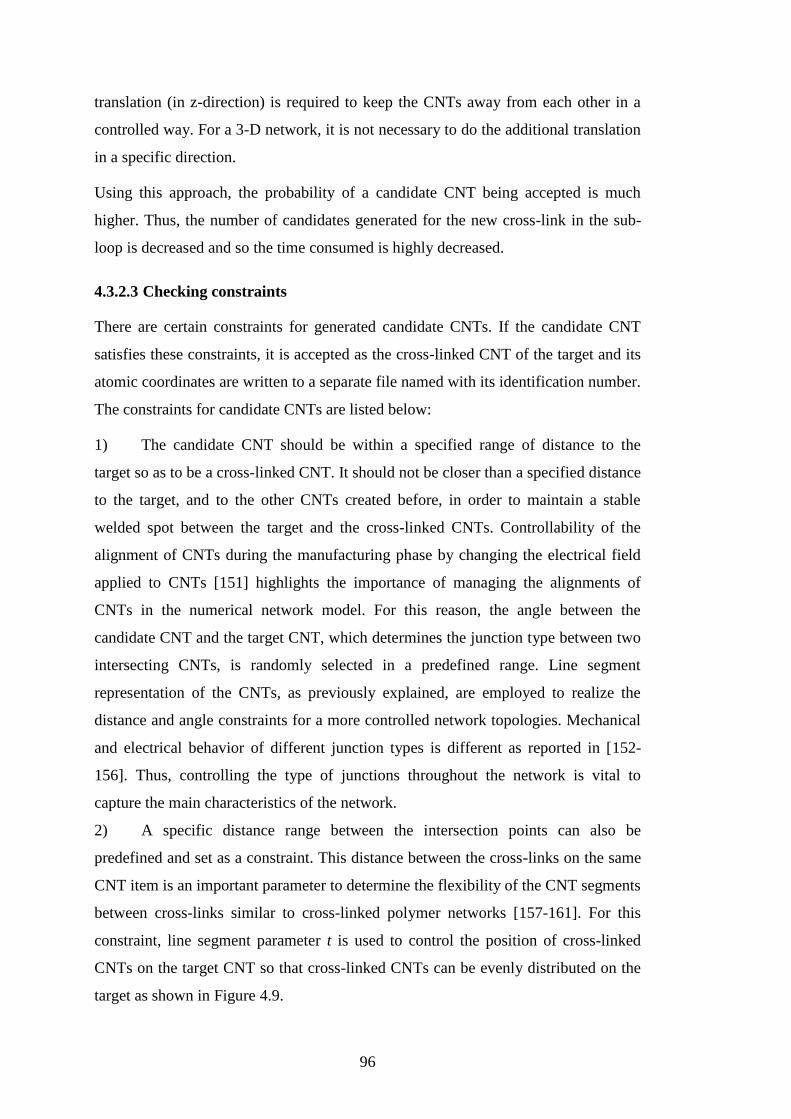
96

translation (in z-direction) is required to keep the CNTs away from each other in a

controlled way. For a 3-D network, it is not necessary to do the additional translation

in a specific direction.

Using this approach, the probability of a candidate CNT being accepted is much

higher. Thus, the number of candidates generated for the new cross-link in the sub-

loop is decreased and so the time consumed is highly decreased.

4.3.2.3 Checking constraints

There are certain constraints for generated candidate CNTs. If the candidate CNT

satisfies these constraints, it is accepted as the cross-linked CNT of the target and its

atomic coordinates are written to a separate file named with its identification number.

The constraints for candidate CNTs are listed below:

1) The candidate CNT should be within a specified range of distance to the

target so as to be a cross-linked CNT. It should not be closer than a specified distance

to the target, and to the other CNTs created before, in order to maintain a stable

welded spot between the target and the cross-linked CNTs. Controllability of the

alignment of CNTs during the manufacturing phase by changing the electrical field

applied to CNTs [151] highlights the importance of managing the alignments of

CNTs in the numerical network model. For this reason, the angle between the

candidate CNT and the target CNT, which determines the junction type between two

intersecting CNTs, is randomly selected in a predefined range. Line segment

representation of the CNTs, as previously explained, are employed to realize the

distance and angle constraints for a more controlled network topologies. Mechanical

and electrical behavior of different junction types is different as reported in [152-

156]. Thus, controlling the type of junctions throughout the network is vital to

capture the main characteristics of the network.

2) A specific distance range between the intersection points can also be

predefined and set as a constraint. This distance between the cross-links on the same

CNT item is an important parameter to determine the flexibility of the CNT segments

between cross-links similar to cross-linked polymer networks [157-161]. For this

constraint, line segment parameter t is used to control the position of cross-linked

CNTs on the target CNT so that cross-linked CNTs can be evenly distributed on the

target as shown in Figure 4.9.

97

Along with these constraints, another constraint can be defined such that the number

of the cross-links interconnected with the target CNT should not be less than the

specified value. This constraint can be relaxed during the generation process. Due to

geometrical difficulties and/or other constraints, sometimes it may be impossible to

place a cross-linked candidate CNT around the target. For this circumstance, this

constraint is relaxed only for the corresponding target to expedite the generation

process. After placing the required number of candidate CNTs on the current target, a

new target CNT is selected among the existing CNTs already generated until the

number of CNTs in the design space exceeds the predetermined value.

All the constraints which will affect the topology of the network can be arranged in

the future according to the detailed characterization results of CNT network

materials. Therefore, the proposed method allows experimental characterization data

to be employed in computer simulations of the materials behavior. Alternatively, the

constraints can be set independently to investigate the effects of several topological

parameters such as CNT lengths between two intersection points, the frequency of

intersections through the network or the angularity of the intersecting CNTs.

4.3.2.4 Making decision

If one of the constraints explained in the previous section is not satisfied, another

candidate CNT is selected from the library, rotated, and translated within the design

space before being checked against the constraints. This sub-loop is kept active until

a suitable candidate satisfying the constraints is found, while the main loop is active

until the specified number of CNTs in the design space is created.

4.3.3 Sample Networks and Welding Procedure

In this section, some examples of 2-D and 3-D CNT network models generated by

stochastic target based algorithm explained elaborately in the previous sections are

presented. In the network models ultra thin CNTs with (5,0) chirality are employed

to ensure the junction formation following the annealing process. In Figure 4.10, the

network generation process is shown by increasing the number of CNT units in the

design space.

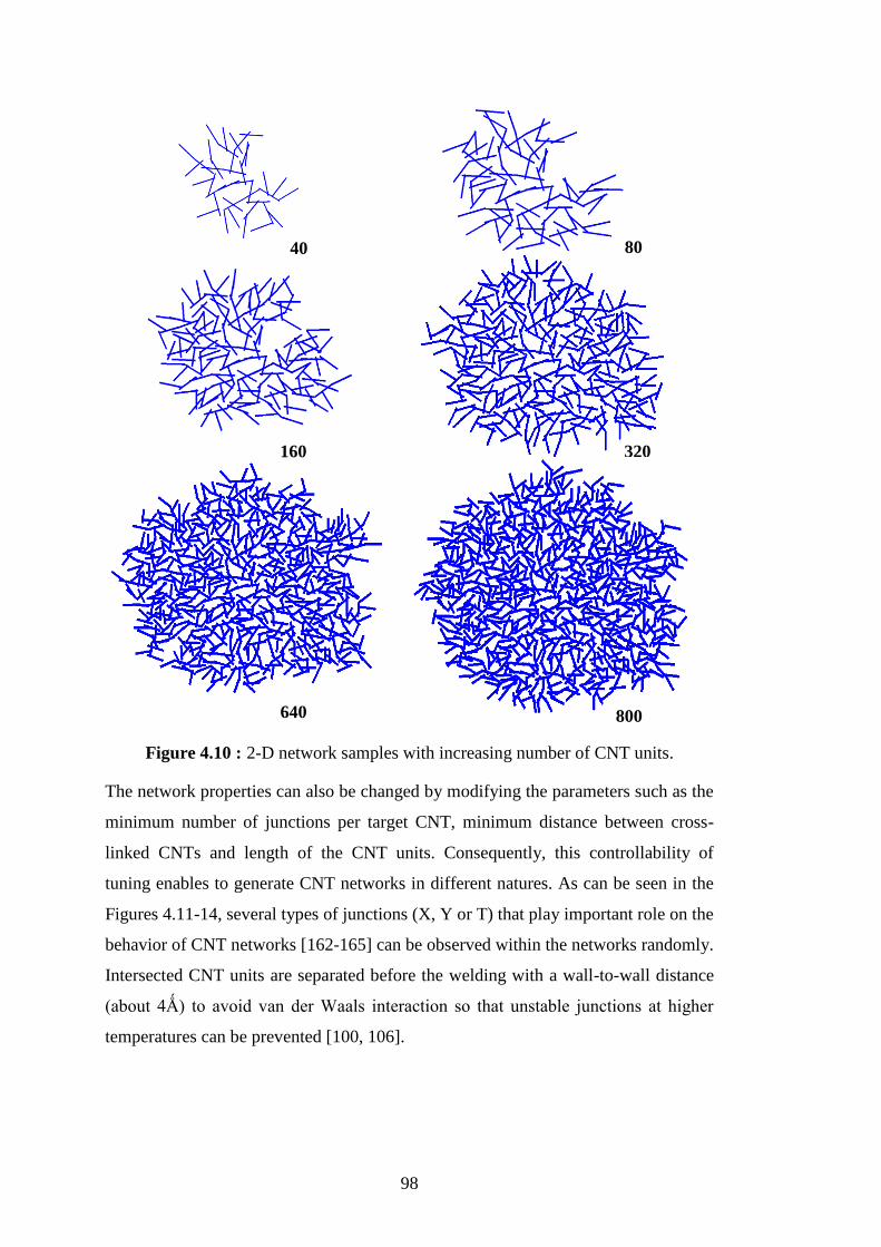
98

Figure 4.10 : 2-D network samples with increasing number of CNT units.

The network properties can also be changed by modifying the parameters such as the

minimum number of junctions per target CNT, minimum distance between cross-

linked CNTs and length of the CNT units. Consequently, this controllability of

tuning enables to generate CNT networks in different natures. As can be seen in the

Figures 4.11-14, several types of junctions (X, Y or T) that play important role on the

behavior of CNT networks [162-165] can be observed within the networks randomly.

Intersected CNT units are separated before the welding with a wall-to-wall distance

(about 4Ǻ) to avoid van der Waals interaction so that unstable junctions at higher

temperatures can be prevented [100, 106].

320 160

40 80

640 800

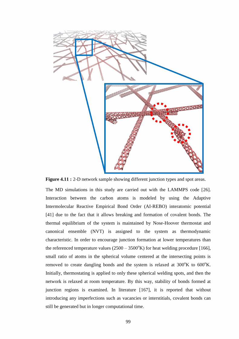
99

Figure 4.11 : 2-D network sample showing different junction types and spot areas.

The MD simulations in this study are carried out with the LAMMPS code [26].

Interaction between the carbon atoms is modeled by using the Adaptive

Intermolecular Reactive Empirical Bond Order (AI-REBO) interatomic potential

[41] due to the fact that it allows breaking and formation of covalent bonds. The

thermal equilibrium of the system is maintained by Nose-Hoover thermostat and

canonical ensemble (NVT) is assigned to the system as thermodynamic

characteristic. In order to encourage junction formation at lower temperatures than

the referenced temperature values (2500 – 3500oK) for heat welding procedure [166],

small ratio of atoms in the spherical volume centered at the intersecting points is

removed to create dangling bonds and the system is relaxed at 300oK to 600

oK.

Initially, thermostating is applied to only these spherical welding spots, and then the

network is relaxed at room temperature. By this way, stability of bonds formed at

junction regions is examined. In literature [167], it is reported that without

introducing any imperfections such as vacancies or interstitials, covalent bonds can

still be generated but in longer computational time.

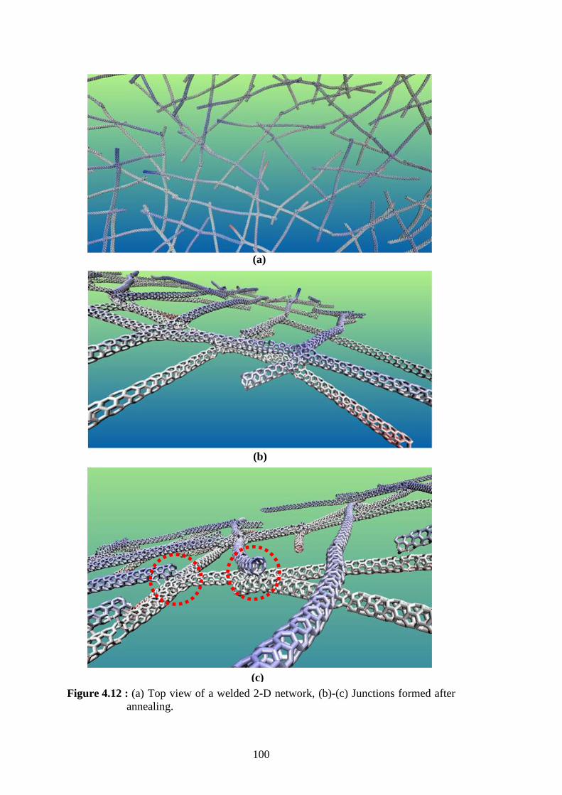
100

Figure 4.12 : (a) Top view of a welded 2-D network, (b)-(c) Junctions formed after

annealing.

(a)

(b)

(c)

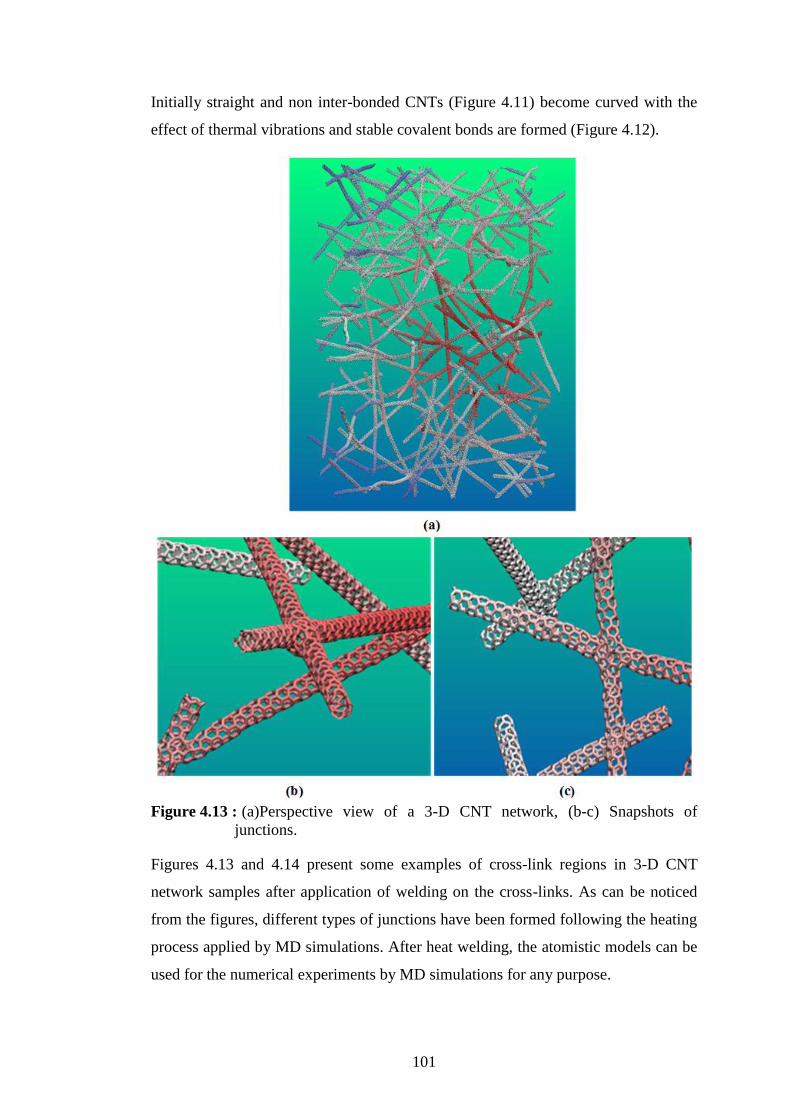
101

Initially straight and non inter-bonded CNTs (Figure 4.11) become curved with the

effect of thermal vibrations and stable covalent bonds are formed (Figure 4.12).

Figure 4.13 : (a)Perspective view of a 3-D CNT network, (b-c) Snapshots of

junctions.

Figures 4.13 and 4.14 present some examples of cross-link regions in 3-D CNT

network samples after application of welding on the cross-links. As can be noticed

from the figures, different types of junctions have been formed following the heating

process applied by MD simulations. After heat welding, the atomistic models can be

used for the numerical experiments by MD simulations for any purpose.

102

Figure 4.14 : Example of junctions throughout 3-D CNT network.

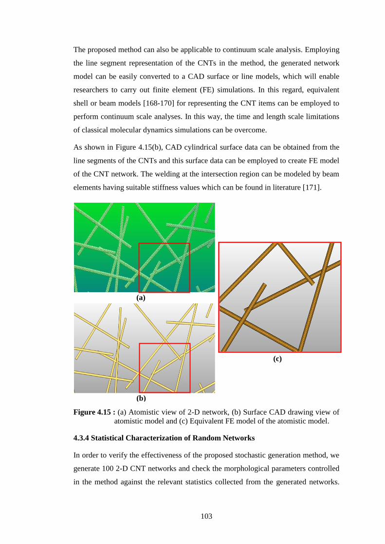
103

The proposed method can also be applicable to continuum scale analysis. Employing

the line segment representation of the CNTs in the method, the generated network

model can be easily converted to a CAD surface or line models, which will enable

researchers to carry out finite element (FE) simulations. In this regard, equivalent

shell or beam models [168-170] for representing the CNT items can be employed to

perform continuum scale analyses. In this way, the time and length scale limitations

of classical molecular dynamics simulations can be overcome.

As shown in Figure 4.15(b), CAD cylindrical surface data can be obtained from the

line segments of the CNTs and this surface data can be employed to create FE model

of the CNT network. The welding at the intersection region can be modeled by beam

elements having suitable stiffness values which can be found in literature [171].

Figure 4.15 : (a) Atomistic view of 2-D network, (b) Surface CAD drawing view of

atomistic model and (c) Equivalent FE model of the atomistic model.

4.3.4 Statistical Characterization of Random Networks

In order to verify the effectiveness of the proposed stochastic generation method, we

generate 100 2-D CNT networks and check the morphological parameters controlled

in the method against the relevant statistics collected from the generated networks.

(a)

(b)

(c)

104

These parameters include the cross link density, angular orientation of cross-linked

CNTs, and distance between two adjacent cross-links. In the verification process,

100 2-D network samples consisted of 100 CNTs of 20 nm in length are realized and

statistically characterized.

Cross-link density, as explained in Section 4.3, is controlled by the parameter that

specifies the expected number of CNTs cross-linked with a target CNT. For the

generated network samples this parameter is chosen to be four for the 20 nm long

CNTs.

Figure 4.16 : (a) Distribution of the number of target CNTs which are completely

cross-linked by 4 CNTs for 100 samples, (b) Distribution of acute

angles (in degree) between cross-linked CNTs in a single sample of

network.

In Figure 4.16 (a), for the 100 networks generated, the distribution of the number of

target CNTs that are cross-linked by four other CNTs in each network is presented.

As mentioned before, when geometrical impossibility emerges during the CNT

generation process, the controlled parameter of four cross-links per target CNT is

relaxed in order to continue to the subsequent steps in the network generation.

Therefore, the maximum number of CNTs that have four cross-links will be less than

total number of CNTs (i.e., 100 in this case). In the current characterization, the

minimum and maximum number of fully covered CNTs are determined to be 86 and

95, respectively, for the 100 CNTs as shown in Figure 4.16 (a). Based on these

results, with the proposed stochastic method, it is shown that the cross-link density

defined as a design parameter can be maintained fairly well in the generated

networks.

For the generated CNT networks, another parameter that is being controlled is the

angular orientation of cross-linked CNTs relative to each other. The angular

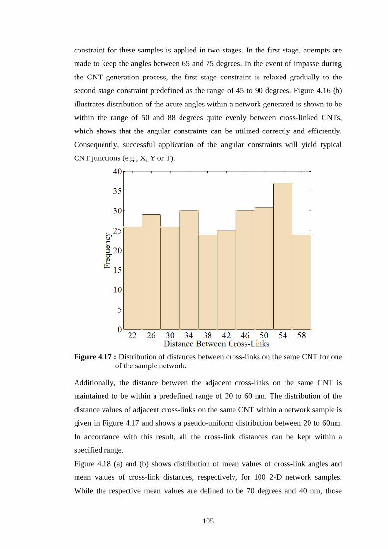
105

constraint for these samples is applied in two stages. In the first stage, attempts are

made to keep the angles between 65 and 75 degrees. In the event of impasse during

the CNT generation process, the first stage constraint is relaxed gradually to the

second stage constraint predefined as the range of 45 to 90 degrees. Figure 4.16 (b)

illustrates distribution of the acute angles within a network generated is shown to be

within the range of 50 and 88 degrees quite evenly between cross-linked CNTs,

which shows that the angular constraints can be utilized correctly and efficiently.

Consequently, successful application of the angular constraints will yield typical

CNT junctions (e.g., X, Y or T).

Figure 4.17 : Distribution of distances between cross-links on the same CNT for one

of the sample network.

Additionally, the distance between the adjacent cross-links on the same CNT is

maintained to be within a predefined range of 20 to 60 nm. The distribution of the

distance values of adjacent cross-links on the same CNT within a network sample is

given in Figure 4.17 and shows a pseudo-uniform distribution between 20 to 60nm.

In accordance with this result, all the cross-link distances can be kept within a

specified range.

Figure 4.18 (a) and (b) shows distribution of mean values of cross-link angles and

mean values of cross-link distances, respectively, for 100 2-D network samples.

While the respective mean values are defined to be 70 degrees and 40 nm, those

106

obtained from the generated networks are 68.9 degrees and 39.8 nm, respectively. As

can be observed from the figures, the scatter around the mean values is very small.

Therefore, it can be concluded that the objective mean values can be captured with

high precision.

Figure 4.18 : (a) Distribution of mean values of cross-link angularity through 100

samples and (b) Distribution of mean values of cross-link distances

through 100 samples.

The above characterization results have demonstrated the effectiveness of the

proposed random network generation method. Hence, networks with tailored

morphology can be accurately generated by setting the parameters controlled in the

method to the appropriate values.

4.4 Investigations on the Mechanical Behavior of CNT Networks

In this section, the studies performed to elaborate the mechanical response of CNT

network materials under tensile loading are given. In this regard, numerical

specimens which are generated by the stochastic method followed by heat welding

process are introduced and numerical settings applied for corresponded MD

simulations are provided. Then, the results obtained through MD simulations are

presented.

4.4.1 Numerical Experiments

In the previous section, a stochastic algorithm developed for the generation of

randomly organized CNT network materials has been explained. By utilizing that

algorithm, several numerical specimens have been generated to investigate the

mechanical behavior of CNT networks under tensile loading conditions. The

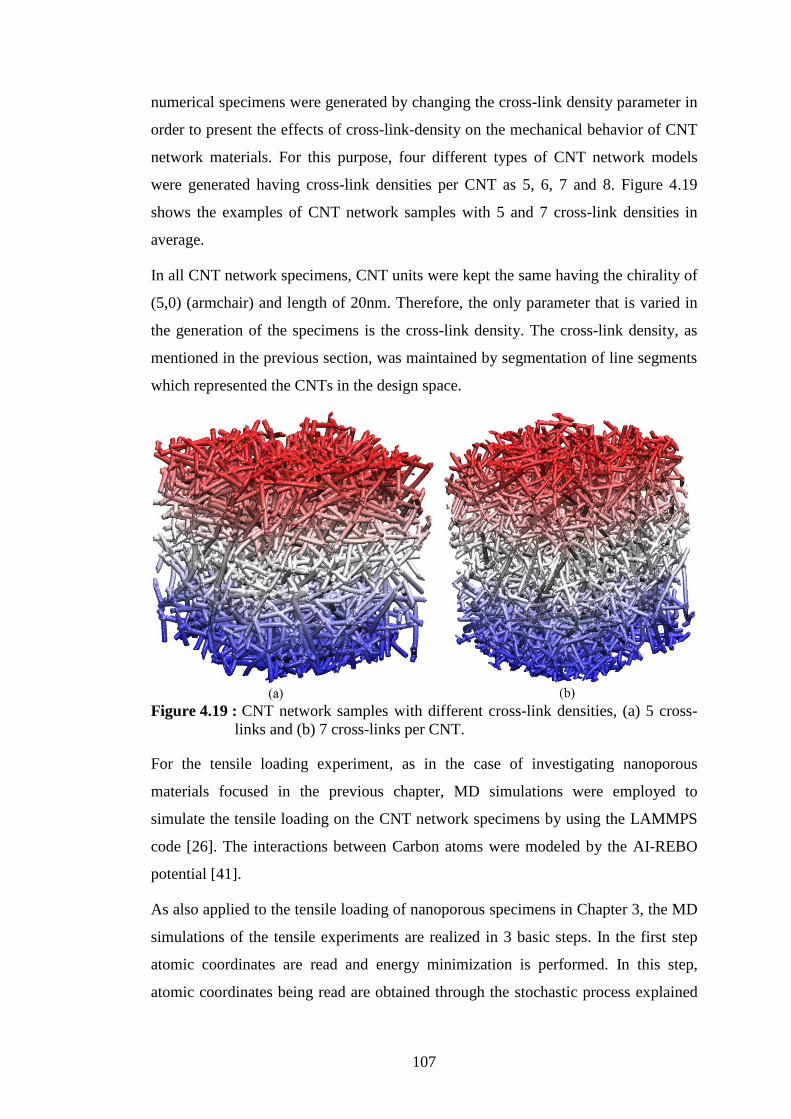
107

numerical specimens were generated by changing the cross-link density parameter in

order to present the effects of cross-link-density on the mechanical behavior of CNT

network materials. For this purpose, four different types of CNT network models

were generated having cross-link densities per CNT as 5, 6, 7 and 8. Figure 4.19

shows the examples of CNT network samples with 5 and 7 cross-link densities in

average.

In all CNT network specimens, CNT units were kept the same having the chirality of

(5,0) (armchair) and length of 20nm. Therefore, the only parameter that is varied in

the generation of the specimens is the cross-link density. The cross-link density, as

mentioned in the previous section, was maintained by segmentation of line segments

which represented the CNTs in the design space.

Figure 4.19 : CNT network samples with different cross-link densities, (a) 5 cross-

links and (b) 7 cross-links per CNT.

For the tensile loading experiment, as in the case of investigating nanoporous

materials focused in the previous chapter, MD simulations were employed to

simulate the tensile loading on the CNT network specimens by using the LAMMPS

code [26]. The interactions between Carbon atoms were modeled by the AI-REBO

potential [41].

As also applied to the tensile loading of nanoporous specimens in Chapter 3, the MD

simulations of the tensile experiments are realized in 3 basic steps. In the first step

atomic coordinates are read and energy minimization is performed. In this step,

atomic coordinates being read are obtained through the stochastic process explained

108

in the previous section and welding process performed at the junctions. In the

minimization process, equilibrium positions of atoms in the systems are received by

finding the minimum of total potential energy of the system in successive iterations.

In the second major step before the application of tensile loading, for the purpose of

incorporating thermal vibrations into the system, or in other words in order to take

into account temperature effects, the system is equilibrated at room temperature. In

the last part, in order to apply tensile loading, tensile displacements are applied to

one end of the atomic structure while the other end is fixed as shown in Figure

3.12(a) in Chapter 3. Therefore, the same tensile loading scheme with the case of

nanoporous simulations is followed for the CNT network simulations.

According to 3 basic stages mentioned above, within an MD simulation of tensile

loading applied to each CNT network specimen, before the application of tensile

loading, an energy minimization process is activated to minimize total energy of the

system to find equilibrium configurations of atoms. This process can be thought as

removing artificial residual stresses from the system to reach relaxed and more stable

equilibrium state. After performing energy minimization on each initial CNT

network specimen, the system was equilibrated at 300oK using the Langevin

thermostat for a total of 10 ps at a time step size of 0.5 fs. Boundary conditions and

stress-strain calculations were performed in the same way as done for nanoporous

simulations explained in the previous chapter. According to that, uniaxial tensile

loading was subsequently applied in one of the principal directions as displacement

boundary condition on one side of the structure over the 1/10 of the total length with

a strain increment of 0.1% that was held constant for 1 ps at 300oK. The other side of

the structure was held fixed while periodic boundary conditions were employed on

all the other sides of the structure. Due to the fact that the strain rate applied to the

specimens affects the mechanical response apparently [172], the same strain rate that

is 109 (1/s) was applied to all specimens. For the purpose of decreasing the noise on

the atomic forces due to thermal fluctuations, stresses were computed based on

atomic forces averaged over 200 time steps spaced uniformly within each strain

increment. At each strain increment, atomic system was equilibrated for 1ps and

atomic forces were averaged for each atom in the last 0.2ps-period of that

equilibration time. Calculated averaged atomic forces were summed to find the total

force at the cross section of the specimen. By this way, total force (P) as shown in

109

Figure 3.11(a) was calculated for each loading/straining step. Classical continuum

equations for stress and strain (Figure 3.11(b)) were employed to calculate stress and

strain values at each load step to generate stress-strain curves for the test specimen.

4.4.2 Results

In tensile loading simulations of CNT network specimens, by dumping out the

atomic coordinates, snapshots of the system could be obtained and thus the progress

of the simulation could be traced. In this regard, several snapshots for the tensile

experiment of CNT network specimen with cross-link density of 7 is given in Figure

4.20. According to this, as the number of loading steps increases, elongation of the

specimen until the rupture can be visualized and any special deformation

mechanisms (if exists) can be observed.

Figure 4.20 : Several instances of CNT network specimen with cross-link density of

7 at different time points in tensile loading simulation.

The most significant observation from the snapshots taken from the tensile

simulations is that deformation of the specimens is initiated by rotation or bending of

CNT segments in the network around cross-links trying to be aligned in the loading

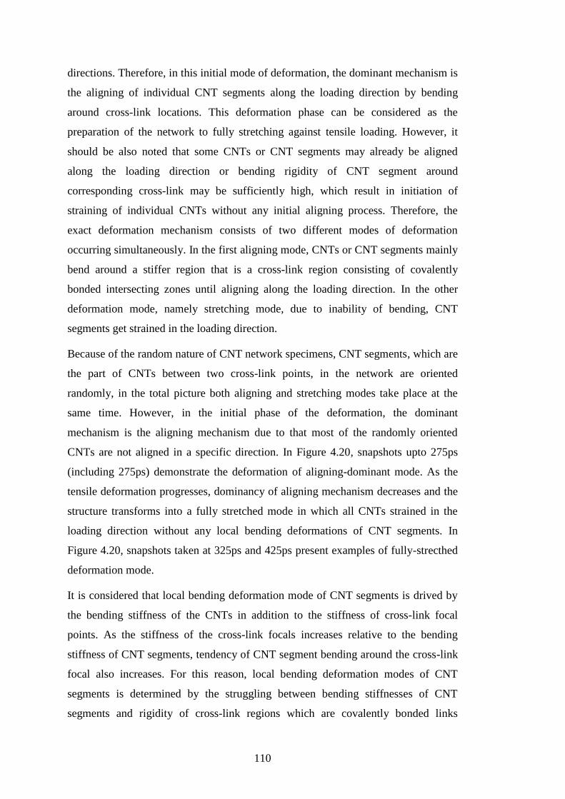
110

directions. Therefore, in this initial mode of deformation, the dominant mechanism is

the aligning of individual CNT segments along the loading direction by bending

around cross-link locations. This deformation phase can be considered as the

preparation of the network to fully stretching against tensile loading. However, it

should be also noted that some CNTs or CNT segments may already be aligned

along the loading direction or bending rigidity of CNT segment around

corresponding cross-link may be sufficiently high, which result in initiation of

straining of individual CNTs without any initial aligning process. Therefore, the

exact deformation mechanism consists of two different modes of deformation

occurring simultaneously. In the first aligning mode, CNTs or CNT segments mainly

bend around a stiffer region that is a cross-link region consisting of covalently

bonded intersecting zones until aligning along the loading direction. In the other

deformation mode, namely stretching mode, due to inability of bending, CNT

segments get strained in the loading direction.

Because of the random nature of CNT network specimens, CNT segments, which are

the part of CNTs between two cross-link points, in the network are oriented

randomly, in the total picture both aligning and stretching modes take place at the

same time. However, in the initial phase of the deformation, the dominant

mechanism is the aligning mechanism due to that most of the randomly oriented

CNTs are not aligned in a specific direction. In Figure 4.20, snapshots upto 275ps

(including 275ps) demonstrate the deformation of aligning-dominant mode. As the

tensile deformation progresses, dominancy of aligning mechanism decreases and the

structure transforms into a fully stretched mode in which all CNTs strained in the

loading direction without any local bending deformations of CNT segments. In

Figure 4.20, snapshots taken at 325ps and 425ps present examples of fully-strecthed

deformation mode.

It is considered that local bending deformation mode of CNT segments is drived by

the bending stiffness of the CNTs in addition to the stiffness of cross-link focal

points. As the stiffness of the cross-link focals increases relative to the bending

stiffness of CNT segments, tendency of CNT segment bending around the cross-link

focal also increases. For this reason, local bending deformation modes of CNT

segments is determined by the struggling between bending stiffnesses of CNT

segments and rigidity of cross-link regions which are covalently bonded links

111

between intersected CNTs generated by the heat welding process in the atomistic

modeling phase.

Following the aligning mode, CNT segments come to a point of locking in which

they cannot continue to their local bending deformation mode. This situation of CNT

segments in which they are fully locked is the initiation of their fully stretched

deformation mode. In the deformation mode of stretching, local bending deformation

mechanisms are not observed anymore. Instead of local bending deformation, all

CNT segments strain individually in the loading direction and the CNT network

specimen finally fails after successive failures of individual CNT segments in the

vicinity of load application region.

Figure 4.21 : Stress-strain curves of CNT network specimens under tensile loading

with different cross-link densities.

As described in the previous chapter, calculations for the values of stress and strain

were performed by using classical continuum equations (see Figure 3.12b) at each

112

load step. The stress-strain curves obtained for the CNT network specimens with

different cross-link densities under tensile loading are shown in Figure 4.21.

According to the stress-strain curves presented in Figure 4.21, apparently it is noticed

that as the number of cross-links increases the stiffness of the CNT networks also

increases. The stiffest specimen, or in other words, the specimen with the highest

Young’s modulus, is easily determined to be the specimen with cross-link density of

8, while the least stiff specimen has the least number of cross-links per CNT.

As observed from Figure 4.21, the Young’s modulus is not the only mechanical

property improved by increasing the cross-link density. The yield and ultimate

strength values of the specimens also increase with increasing number of cross-link

densities. Because there were no obvious transitions from linearity so the values of

yield points have been approximated conventionally by finding the intersection of the

stress-strain curve with a line parallel to the initial slope of the curve and which

intercepts the abscissa at 0.2%. Moreover, ultimate strain, which is the measure of

maximum elongation, increases as the cross-link density increases. The quantitative

evaluation of the numerical experiments on the CNT network specimens with

different cross-link densities is given in Table 4.3.

Summary of quantitative results from tensile loading simulations. Table 4.3 :

Cross-Link

Density

Density

(g/cm3)

Modulus

(GPa)

Yield Strength

(MPa)

Ultimate

Strain (%)

5 0.45 14.55 2006 32

6 0.53 18.96 2935 36

7 0.61 24.35 4248 38

8 0.83 37.00 5200 47

As the cross-link density increases, CNT segment lengths decrease while the

percolation through the network increases due to increased connectivity between the

CNTs. Because cross-links represent the interconnectivity between the CNTs in the

network, the load distribution is more homogenous at higher cross-link densities

through the network comparing with lower cross-link densities. Due to increased

load-sharing capability, interconnection in the network increase as well, which, in

turn, increases the number of CNT segments bearing the applied load. Eventually,

mechanical properties are improved.

Naturally, as the cross-link density increases, density of the specimens is also

elevated. However, stiffness increase rate by cross-link density increase is higher

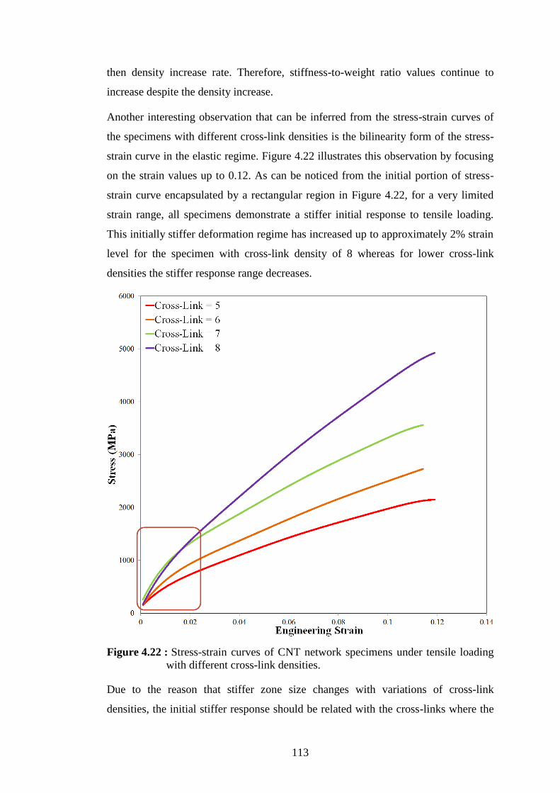
113

then density increase rate. Therefore, stiffness-to-weight ratio values continue to

increase despite the density increase.

Another interesting observation that can be inferred from the stress-strain curves of

the specimens with different cross-link densities is the bilinearity form of the stress-

strain curve in the elastic regime. Figure 4.22 illustrates this observation by focusing

on the strain values up to 0.12. As can be noticed from the initial portion of stress-

strain curve encapsulated by a rectangular region in Figure 4.22, for a very limited

strain range, all specimens demonstrate a stiffer initial response to tensile loading.

This initially stiffer deformation regime has increased up to approximately 2% strain

level for the specimen with cross-link density of 8 whereas for lower cross-link

densities the stiffer response range decreases.

Figure 4.22 : Stress-strain curves of CNT network specimens under tensile loading

with different cross-link densities.

Due to the reason that stiffer zone size changes with variations of cross-link

densities, the initial stiffer response should be related with the cross-links where the

114

CNTs are interconnected with each other by covalent bonds. Therefore, this initially-

stiffer behavior can be attributed to the stiffer response of cross-link regions that

cease after a limited straining of the specimens. This observation can also be

explained by a possible requirement of extra strain energy imparted to the covalently

bonded cross-links to activate and motivate the deformation.

In order to investigate the mechanical behavior of CNT networks further, another

principle loading type, that is shear loading, was applied on the same CNT network

specimens with cross-link densities of 6, 7 and 8. Same MD settings with tensile

simulations have been used for the those shear loading simulations while the only

change is the loading direction.

Figure 4.23 : Several instances of CNT network specimen with cross-link density of

6 at different time points in shear loading simulation.

Figure 4.23 illustrates several snapshots of shear loading simulation performed for

the CNT network specimen with cross-link density of 6. Examining the shear

deformation of CNT networks through MD simulation snapshots showed that

displacement of atoms in the shearing direction initiated at the top where the shear

loading was applied, while the atoms located sufficiently away from the top were not

affected by shearing. As the shear loading is kept actively applied on the specimen,

bending deformation of individual CNTs resulted in aligning of CNTs along the

shearing direction. When the CNTs that are closest to the loading plane deformed by

bending, shear effect transmitted to the lower network regions away from the loading

115

planes through covalently bonded CNT cross-links. In this way, shear load is

transmitted to the all network resulting in collective shear deformation. When the

shear loading effect disffuses into overall structure of the CNT network specimen,

shear deformation continues with collective shearing of the total system. The final

failure of the specimen due to shear loading occurs following the collective shear

deformation of the specimen at the region closest to shear plane. This deformation

behavior can also be observed from the snapshots provided in Figure 4.23.

According to this, at the time point of 125ps, it is clearly noticed that shear loading

effect is partially diffused into the network system, so only a portion of the specimen

is deformed locally in the shear loading direction. As the loading is kept active, at the

time point of 275ps, a larger portion of the specimen comparing to the time point of

125ps is deformed in the shearing direction. At the time point of 425ps, it is seen that

shear loading effect has been distributed to the all structure and a collective or global

shear deformation is observed. As a consequence of global shear deformation

process, at the time point of 725ps, the network structure fails by fracture formations

at the upper portion of the specimen close to the loading plane.

Figure 4.24 : Stress-strain curves of CNT network specimens under shear loading of

the specimens with the cross-link densities of 5 and 6.

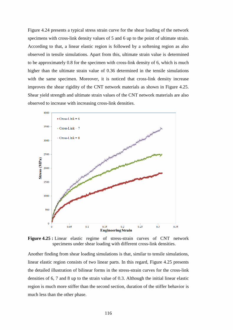
116

Figure 4.24 presents a typical stress strain curve for the shear loading of the network

specimens with cross-link density values of 5 and 6 up to the point of ultimate strain.

According to that, a linear elastic region is followed by a softening region as also

observed in tensile simulations. Apart from this, ultimate strain value is determined

to be approximately 0.8 for the specimen with cross-link density of 6, which is much

higher than the ultimate strain value of 0.36 determined in the tensile simulations

with the same specimen. Moreover, it is noticed that cross-link density increase

improves the shear rigidity of the CNT network materials as shown in Figure 4.25.

Shear yield strength and ultimate strain values of the CNT network materials are also

observed to increase with increasing cross-link densities.

Figure 4.25 : Linear elastic regime of stress-strain curves of CNT network

specimens under shear loading with different cross-link densities.

Another finding from shear loading simulations is that, similar to tensile simulations,

linear elastic region consists of two linear parts. In this regard, Figure 4.25 presents

the detailed illustration of bilinear forms in the stress-strain curves for the cross-link

densities of 6, 7 and 8 up to the strain value of 0.3. Although the initial linear elastic

region is much more stiffer than the second section, duration of the stiffer behavior is

much less than the other phase.

117

Shear modulus values calculated for two stage values are given in Table 4.4.

Quantative description of shear modulus values for two different stages has shown

that shear modulus in the initial elastic phase is approximately 6 times of the second

phase.

Summary of quantitative results from shear loading simulations. Table 4.4 :

Cross-Link

Density

Density

(g/cm3)

Shear Modulus (1st

Stage)(GPa)

Shear Modulus (2nd

Stage)(GPa)

6 0.53 24.96 4.45

7 0.61 36.91 5.86

8 0.83 42.60 7.20

The bilinaerity of stress-strain relationship in the elastic region, which was also

observed in the tensile response of the CNT networks, has been inferred to the

required work to activate the individual CNTs to initiate the deformation for their

aligning along the shear or tensile loading direction. Because this initial activation of

the deformation is related to the stretching of the individual CNTs, it represents a

higher stiffness comparing with bending deformation of CNT segments which are

observed after the initial activation of the deformation.

4.5 Summary and Conclusion

In this chapter, a stochastic algorithm has been developed to model 2-D and 3-D

CNT networks with random geometrical parameters such as CNT orientation and

intersection angles. While some parameters are allowed to be random in nature, some

parameters such as CNT chirality and length scale, cross-link or junctional density,

angular limits for the intersections of two CNTs can be managed independently. In

this way, several CNT network specimens with controlled structural parameters were

able to be generated. CNT intersecting regions through CNT networks with the

proposed method were welded following canonical MD simulations by heating and

stable covalent bond formations could be obtained. The sample CNT network models

generated by the proposed technique have been provided illustrating that generated

samples represent the basic characteristics of CNT networks such as X, Y and T type

of junctions formed between cross-linked CNTs. Finally, 2-D or 3-D CNT networks

are generated with controllable parameters and can be employed for further

mechanical, electrical or thermal studies. Due to the controllability and efficiency on

the topological features of CNT networks and simplicity of the generation algorithm,

118

this CNT network generation method may significantly increase the numerical and

theoretical investigations on the CNT networks.

The generation method proposed for the atomistic models of CNT networks is also

applicable to continuum scale analyses in order to overcome the time and length

scale limitations of classical MD simulations. Due to line segment representation of

CNTs in the method, the generated network model can be easily converted to a CAD

surface or line models, which will enable researchers to carry out FE simulations.

Furthermore, following this study, mechanical, thermal or electrical properties of

CNT networks can be optimized by changing the topological parameters, and

manufacturing techniques can be developed or improved to produce optimized

networks.

CNT network specimens generated by the developed technique have been employed

to investigate mechanical behavior of CNT network materials. For this purpose,

several CNT network specimens with different cross-link densities were utilized in

MD simulations by applying tensile loading. Results of MD simulations showed that

mechanical properties of CNT networks including Young’s modulus, yield and

ultimate tensile strength could be improved by increasing the cross-link density.

Total elongation values of the specimens were also demonstrated to increase with

cross-link density. Moreover, by tracking of tensile experiments in MD simulations,

two different deformation modes, which are the modes of aligning and fully-

stretching, have been identified. Moreover, it has been observed that the total

deformation of the network is composed of two modes, while aligning mode is

dominant at the initial phase up to straining of all CNT segments in the loading

direction. In addition to tensile loading simulations, shear loading simulations have

also been performed by using the same MD simulation parameters with tensile

simulations. Similar to the results obtained through tensile loading experiments, it

has been shown that cross-link density increase yields better mechanical performance

in terms of shear modulus, shear yield strength and ultimate shear strain. In the

regard of deformation mechanisims, it has been illustrated that shear deformation of

the specimens starts from the loading plane and diffuses into the all structure in a

progressive manner. Furthermore, bilinearity form of the stress-strain curves under

shear loading, which has also been observed in tensile loading simulations, has been

119

quantitatively and graphically presented. According to that the bilinear form of stress

strain curves has been explained by the initial activation of deformation

121

5. CONCLUSIONS AND RECOMMENDATIONS

Day after day nanoscience and nanotechnology bring out new and novel materials

that are capable of performing incredibly much better than conventional materials

due to their exceptional physical and chemical properties. CNT network and

nanoporous materials are amazing examples of those novel materials having nano-

organized structures. Both CNT network and nanoporous materials are built up

randomly organized structural units that are CNTs in the case of CNT network

materials while ligaments and junctions in the case of open cell nanoporous

materials. Because of their complex morphologies arising from their random natured

atomistic organization, it is highly challenging to numerically model these materials,

which avoids increased number of computational experiments exploring their

material properties. It would be very beneficial to develop such techniques that

enable to generate atomistic models of those materials to investigate the effects of

morphological parameters on their material properties. With this motivation, in the

content of this dissertation, as the first stage of the study, stochastic models are

developed for random natured nanomaterials such as CNT networks and nanoporous

materials which have extraordinary properties including ultra-high stiffness-to-

weight ratios that make them candidates in a broad range of applications.

In the regard of CNT network modeling, a stochastic algorithm is developed to

model 2-D and 3-D CNT networks with random geometrical parameters such as

CNT orientation and intersection angles. While some parameters are let to be random

in nature, some behavior decisive parameters such as CNT chirality and length scale,

cross-link density, angular limits for intersections can be kept under control, which

enable to generate different models organized with different parameters. It should be

noted here that the approach of considering the CNTs as line segments during the

generation process save a lot of computational time for the generation of total

network structure. Following the generation of a CNT network in which the CNT

units are so close to each other that heating to certain temperatures can yield

covalently bonded cross-links, classical molecular dynamics simulations are carried

122

out to obtain covalently bonded networks. Finally, 2-D or 3-D CNT networks were

generated with controllable parameters and could be employed for further

mechanical, electrical or thermal studies. Due to the controllability and efficiency on

the topological features of CNT networks and simplicity of the generation algorithm,

this CNT network generation method may significantly increase the numerical and

theoretical investigations on the CNT networks.

The method proposed for the modeling of CNT networks is also applicable to

continuum scale analyses in order to overcome the time and length scale limitations

of classical molecular dynamics simulations. By the help of line segment

representation of the CNTs in the method, the generated network model can be easily

converted to a CAD surface or line segment model, which will enable researchers to

carry out FE simulations. By this way, availability of the proposed method to be used

in classical continuum scale computational studies enlarges the applicability zone of

the method. Beside that, the proposed method for the generation of CNT networks,

can be utilized or at least can be used as a base idea for the generation of similar

network materials which consist of one dimensional structural units that can be

idealized as line segments. For example, in the computational modeling of polymeric

materials that consist of linear polymer chains, the proposed algorithm may be an

ideal inspiration source. Furthermore, following this study, mechanical, thermal or

electrical properties of CNT networks can be optimized by changing the topological

parameters, and manufacturing techniques can be developed or improved to produce

optimized networks.

For the modeling of nanoporous materials, with the spherical cell shape assumption,

randomly intersected speherical ensembles are employed to generate nanoporous

materials. Within the scope of the developed algorithm, by controlling the several

parameters such as maximum and minimum number of spheres intersected to each

sphere and maximum overlapping ratio between two intersected spheres, the porosity

of the nanoporous systems can be arranged to generate desired nanoporous

specimens with desired porosity values. In the meantime, some parameters that can

be kept under control help to obtain different ranges of ligament size, which is

another direct control on the morphology of nanoporous structures. Central

coordinates and radii of spheres existing in the ensemble that is formed by randomly

intersection of spheres are employed in atomistic modeling software to remove atoms

123

encapsulated by the spherical volumes from a crystalline solid block. As a result, by

utilizing this technique atomistic models of nanoporous materials can be generated

by controlling the key parameters affecting the morphology so the behavior of the

structure with the spherical shape assumption of pores.

Applicability of both stochastic algorithms developed for CNT networks and

nanoporous materials is shown by demonstrating the specimen samples having the

proposed morphological characteristics such as porosity and cross-links for

nanoporous and CNT network materials, respectively. For example, for CNT

network specimens it is shown that through the network consisting of randomly

intersected CNTs, several junction types that are already characterized in literature

such as X, Y or T junctions could be generated by the proposed method following

the heat welding process realized within molecular dynamics simulations. In the

same manner, regarding nanoporous material modeling, it is demonstrated that basic

features of a cellular structure such as ligaments, cell walls, pores on the cell walls

and junctions could be obtained as a result of realizing the proposed method.

More importantly than showing the validity of proposed algorithms developed for the

random atomistic structures, generated numerical specimens for both materials by

using the developed techniques are used in molecular dynamics simulations to

perform tensile loading experiments. As a result of MD simulations, stress-strain

plots have been obtained and by evaluating stress-strain behavior from those plots,

different aspects in deformation mechanisms of corresponded materials have been

explained. For instance, regarding nanoporous numerical specimens it has been

verified that as the porosity of the specimens increases the major mechanical

properties including Young’s modulus, yield and ultimate tensile strength of the

nanoporous materials decreases. Beside this, a notable decrease in softening rate after

a specific porosity value has been discovered and this significant softening rate

decrease at higher porosity values has been devoted to more homogenous stress

distribution due to increased compliance between ligaments and junctions. In order

to verify this, von Mises stress distribution of the networks for two different

porosities having distinctive softening rates have been compared. While in the

specimen with lower porosity the high stress spot areas are cumulated around the

upper edge location, for the sample with higher porosity peak stress focals are

distributed more evenly. The reason for such a behavior has been explained by the

124

microstructural compliance issue between ligaments and junction. Thus, it has been

concluded that as the porosity decreases stress flow through incompatible junctions

and ligaments becomes more difficult to spread out, which in turn results in higher

peak stress locations close to load application region. Similarly, stress-strain plots for

CNT network specimens have been obtained through MD simulations and shown

that as the cross-link density increases, Young’s modulus, yield and ultimate tensile

strength of CNT networks have been improved. Moreover, deformation mechanisms

of CNT networks under tensile loading have been identified by illustrating

deformation snapshots taken from the MD simulations while the tensile loading was

in progress. In this regard, two main deformation styles have been defined to explain

the characteristics of deformation mechanisms. One of these, aligning type of

deformation has been referred for the local bending deformations of CNT segments

around relatively more rigid regions which are mostly cross-links. The other type of

deformation has been named as stretching mode of deformation, in which the CNT

segments are subjected to straining in the loading direction without any bending

deformation. In conclusion, it has been underlined that the tensile deformation of

CNT networks from the global windows proceeds with the combination and

interaction of these two deformation styles.

The most important findings from the numerical experiments of the atomistic models

which were generated by the presented techniques are the tips that might enable

researchers to produce advanced materials with improved properties. For example,

regarding nanoporous materials, in this dissertation it has been stated that as the

compatibility between junctions and ligaments are increased, load bearing capacity

of the porous network can be increased with more uniform lower-level stress

distribution comparing to incompatible ligaments and junctions. Therefore, the

importance of compliance between structural units within the porous network has

been pointed out by this way. In the same way, a similar finding for CNT network

materials has been demonstrated by explaining the two different local deformation

styles. In this regard, as the period of local bending deformation mode of the CNTs is

increased before that the stretching mode turns into dominant mechanism the total

elongation of the structure can be increased, which results in improved mechanical

performance.

125

The studies performed in this dissertation can be utilized in the future works for the

further investigations on the structure-material relationship of especially randomly

organized nanostructured materials. In this respect, first of all, the proposed atomistic

model generation techniques for both CNT networks and nanoporous materials can

be employed to investigate the effects of other controlled paramaters on the

mechanical performance. For instance, in this dissertation effects of porosity and

cross-link density have been studied for nanoporous and CNT network materials,

respectively. In the future studies, other parameters including effect of cell diameters

for nanoporous materials and CNT chirality or CNT length scale for CNT network

materials can be varied to explore their effects on the mechanical performance.

Furthermore, other physical properties such as thermal properties of the materials can

also be investigated in terms of the effects of controlled parameters (e.g., porosity,

cross-link density) on the desired property. Therefore, the output of this study

performed in this dissertation is not only useful or applicable to the investigation of

mechanical properties, because of the reason that stochastic atomistic models can be

employed in MD simulations for all purposes.

In this dissertation, only 3-D CNT network models have been employed in MD

simulations for the investigation of mechanical properties. However, the proposed

technique for the generation of random natured CNT networks can also be applicable

to generate 2-D network models representing CNT films. As a result, computational

experiments on CNT films can be conducted to explore their structure dependent

properties and to find tips for manufacturing optimum structures.

Another research opportunity arising from this dissertation is the investigation on the

effects of coating of nanoporous materials on the mechanical or thermal behavior of

nanoporous materials. The stochastic method developed for the generation of

atomistic structure of nanoporous structures can be easily improved to generate

coated version of nanoporous structures and then the atomistic models can be used

for any purpose of numerical experiments in MD simulations. Similarly, nanoporous

models can be filled with another material to explore its effects on the mechanical

properties as well as thermal properties.

127

REFERENCES

[1] Yousaf, A. A. & Ali, S. (2008). Why nanoscience and technology?What is

there for us? J. Fac. Eng. &Tech., 11-20.

[2] Rao, C. N. R., Muller, A., & Cheetham, A. K. (2004). Chemistry of

nanomaterials. Weinheim: Wiley-VCH.

[3] Rao, C. N. R. & Cheetham, A. K. (2001). Science and technology of

nanomaterials. J. Mater. Chem., 11, 2887-2892.

[4] Seigel, R. W., Hu, H., & Roco, M.C. (1999). Nanostructures science and

technology. Boston: Kluwer Academic Publishers.

[5] Roco, M. C., Williams, R. S., & Alivisatos, A. P. (2000). Nanotechnology

research directions. Boston: Kluwer Academic Publishers.

[6] Manasreh, O. (2012). Introduction to nanomaterials and devices. Hoboken,

NJ: John Wiley & Sons.

[7] Edelstein, A. S. & Cammaratra, R. C. (1996). Nanomaterials: Synthesis,

properties and applications (2nd ed.). New York, NY: Taylor &

Francis.

[8] Ajayan, P. M., Schadler, L. S., & Braun, P. V. (2004). Nanocomposite

science and technology. Weinheim: Wiley.

[9] Gogotsi, Y. (2006). Carbon nanomaterials. Boca Raton,FL: CRC Press.

[10] O’Connell, A.J. (2006). Carbon nanotubes properties and applications. Boca

Raton, FL: CRC Press.

[11] Pokripivny, V., Lohmus, R., Hussainova, I., Pokropivny, A., & Vlassov, S.

(2007). Introduction to nanomaterials and nanotechnology. Tartu:

Tartu University Press.

[12] Binns, C. (2010). Introduction to nanoscience and nanotechnology. Hoboken,

NJ: John Wiley & Sons.

[13] Tanaka, K., Yamabe, T., & Fukui, K. (1999). The science and technology of

carbon nanotubes (1st ed.). Oxford: Elsevier Ltd.

[14] Hornyak, G. L., Dutta, J., Tibbals, H. H., & Rao, A. K. (2008). Introduction

to nanoscience. Boca Raton, FL: CRC Press.

[15] Iijima, S., & Ichihashi, T. (1993). Single-shell carbon nanotubes of 1-nm

diameter. Nature, 363, 603-605.

[16] Bethune, D. S., Klang, C. H., Vries, M. S., Gorman, G., Savoy, R.,

Vazquez, J., & Beyers, R. (1993). Cobalt-catalysed growth of carbon

nanotubes with single atomic-layer walls. Nature, 363, 605-607.

[17] Iijima, S. (1991). Helical microtubules of graphitic carbon. Nature, 354, 56-58.

128

[18] Vollath, D. (2008). Nanomaterials: an introduction to synthesis, properties

and applications. Weinheim: Wiley-VCH.

[19] Guozhong, C. (2004). Nanostructures & Nanomaterials: Synthesis, properties

& applications. London: Imperial College Press.

[20] Schodek, D. L, Ferreira, P., & Ashby, M. F. (2009). Nanomaterials,

nanotechnologies and design: An introduction for engineers and

architects. Oxford: Elsevier Ltd.

[21] Singh, S. C., Zeng, H. B., Guo, C., & Cai, W. (2012). Nanomaterials.

Weinheim: Wiley-VCH.

[22] Jackson, M. J. (2006). Microfabrication and nanomanufacturing. Boca Raton,

FL: CRC Press.

[23] Busnaina, A. (2006). Nanomanufacturing handbook. Boca Raton, FL: CRC

Press.

[24] Lu, G. Q, & Zhao, X. S. (2004). Nanoporous materials: An overview. In G. Q

Lu & Zhao X.S. (Eds.), Nanoporous Materials: Science and

Engineering (Vol.4, pp.1-12). London, UK: Imperial College Press.

[25] Polarz, S., & Smarsly, B. (2002). Nanoporous materials. Journal of

Nanoscience and Nanotechnology, 2 (6), 581-612.

[26] Plimpton, S. (1995). Fast parallel algorithms for short-range molecular-

dynamics. J. Comput. Phys., 117, 1-19.

[27] Alder, B. J. & Wainwright, T. E. (1959). Studies in molecular dynamics. i.

general method. J. Chem. Phys., 27, 1208-1216.

[28] Gibson, J. B., Goland, A. N., Milgram, M., & Vineyard, G. H. (1960).

Dynamics of radiation damage. Phys. Rev., 120, 1229-1253.

[29] Rahman, A. (1964). Correlations in the motion of atoms in liquid argon. Phys.

Rev., 136, A405-A411.

[30] Weiner, S. J., Kollman, P. A., Case, D. A., Singh, U. C., Ghio, C., Alagona,

G., … Weiner, P. (1984). A new force-field for molecular

mechanical simulation of nucleic acids and proteins. J. Am. Chem.

Soc., 106, 765-784.

[31] Frenkel, D. & Smit, B. (2002). Understanding Molecular Simulation: From

Algorithms to Applications (2nd ed.). San Diego, CA: Academic

Press.

[32] Tobias, D. J., Martyna, G. J., & Klein, M. L. (1993). Molecular dynamics

simulations of a protein in the canonical ensemble. J. Phys. Chem.,

97, 12959-12966.

[33] Maitland, G. C., Rigby, M., Smith, E. B., & Wakeham, W. A. (1981).

Intermolecular forces:their origin and determination. Oxford:

Clarendon Press.

[34] Stone, A. J. (1996). The theory of intermolecular forces. Oxford: Clarendon

Press.

[35] Evans, D. J. & Morriss, G. P. (1990). Statistical mechanics of nonequilibrium

liquids. London: Academic Press.

129

[36] Andersen, H. C. (1980). Molecular dynamics simulations at constant pressure

and/or temperature. J. Chem. Phys., 72, 2384-2393.

[37] Deleeuw, S. W., Perram, J. W., & Petersen, H.G. (1990). Hamilton

equations for constrained dynamics systems. J. Stat. Phys., 61, 1203-

1222.

[38] Verlet, L. (1967). Computer experiments on classical fluids. i.

thermodynamical properties of Lennard-Jones molecules. Phys. Rev.,

159 , 98-103.

[39] Daw, M.S. & Baskes, M.I. (1984). Embedded-atom method: Derivation and

application to impurities, surfaces, and other defects in metals. Phys.

Rev. B, 29, 6443-6453.

[40] Stuart, S. J., Tutein, A. B., & Harrison, J. A. (2000). A reactive potential for

hydrocarbons with intermolecular interactions. J. Chem. Phys., 112,

6472-6486.

[41] Brenner, D. W., Shenderova, O. A., Harrison, J. A., Stuart, S. J., Ni, B., &

Sinnott, S. B. (2002). A second-generation reactive empirical bond

order (REBO) potential energy expression for hydrocarbons. Phys.

Rev. B, 14, 783-802.

[42] Gibson, L. J. & Ashby, M. F. (1997). Cellular Solids: Structures and

Properties (2nd ed.). Cambridge, England: Cambridge University

Press.

[43] Bonroy, K., Friedt, J. -M, Frederix, F., Laureyn, W., Langerock, S.,

Campitelli, A., …Declerck, P. (2004). Realization and

characterization of porous gold for increased protein coverage on

acoustic sensors. Anal. Chem., 76, 4299.

[44] Weissmüller, J., Viswanath, R. N., Kramer, D., Zimmer, P., Wuereschum,

R., & Gleiter, H. (2003). Charge-induced reversible strain in a metal.

Science, 300, 312.

[45] Hodge, A. M., Biener, J., Hayes, J. R., Bythrow, P. M., Volkert, C. A., &

Hamza, A. V. (2007). Scaling equation for yield strength of

nanoporous open-cell foams. Acta Mater., 55, 1343-1349.

[46] Sun, X. Y., Xu, G. K., Li, X., Feng, X. Q., & Gao, H. (2013). Mechanical

properties and scaling laws of nanoporous gold. J. Appl. Phys., 113,

023505-9.

[47] Farkas, D., Caro, A., Bringa, E., Crowson, D. (2013). Mechanical response

of nanoporous gold. Acta Materialia, 61, 3249-3256.

[48] Sun, Y., Ye, J., Shan, Z., Minor, A.M., Balk, T.J. (2007). The Mechanical

Behavior of Nanoporous Gold Thin Films. JOM, 59, 54-58.

[49] Zhu, H. X., Knott, J. F., & Mills, N. J. (1997). Analysis of the elastic

properties of open-cell foams with tetrakaidecahedral cells. Journal of

the Mechanics and Physics of Solids, 45, 319-343.

[50] Warren, W. E., & Kraynik, A. M. (1988). Linear elastic properties of open-

cell foams. Journal of Applied Mechanics, 55, 341-346.

http://dx.doi.org/10.1021/ac049893u

http://dx.doi.org/10.1021/ac049893u

http://dx.doi.org/10.1126/science.1081024

http://dx.doi.org/10.1016/j.actamat.2006.09.038

130

[51] Duria, D. J. (1997). Bubble-scale model of foam mechanics: Melting,

nonlinear behavior, and avalanches. Physical Review E, 55, 1739-

1751.

[52] Xia, R., Xu, C. X., Wu, W. W., Li, X., Feng, X. Q., & Ding, Y. (2009).

Microtensile tests of mechanical properties of nanoporous Au thin

films. Journal of Materials Science, 44, 4728–4733.

[53] Li, R. & Sieradzki, K. (1992). Ductile-brittle transition in random porous Au.

Phys. Rev. Lett., 68, 1168-1178.

[54] Erlebacher, J., Aziz, M. J., Karma, A., Dimitrov, N., & Sieradzki, K.

(2001). Evolution of nanoporosity in dealloying. Nature, 410, 450-

453.

[55] Kramer, D., Viswanath, R. N., & Weissmüller, J. (2004). Surface-stress

induced macroscopic bending of nanoporous gold cantilevers. Nano

Letters, 4, 793.

[56] Ganguly, P. & Ulm, F. –J. (2007). Analysis of deformation coupled surface

remodeling in porous biomaterials. J. Mater. Sci., 42, 8873.

[57] Kaneko K. (1994). Determination of pore size and pore size distribution: 1.

Adsorbents and catalysis. Journal of Membrane Science, 96, 59-89.

[58] Hakamada, M. & Mabuchi, M. (2007). Mechanical strength of nanoporous

gold fabricated by dealloying. Scr. Mater., 56, 1003-1009.

[59] Zhang, W. X. & Wang, T. J. (2007). Effect of surface energy on the yield

strength of nanoporous materials. Appl. Phys. Lett., 90, 063104.

[60] Mathur, A. & Erlebacher, J. (2007). Size dependence of effective Young’s

modulus of nanoporous gold. Appl. Phys. Lett., 90, 061910.

[61] Biener, J., Hodge, A. M., & Hamza, A. V. (2005). Microscopic failure

behavior of nanoporous gold. Appl. Phys. Lett., 87, 121908.

[62] Kirca, M., Gul, A., Ekinci, E., Yardim, F., & Mugan, A. (2007).

Computational modeling of micro-cellular carbon foams. Finite Elem.

Anal. Des., 44, 45-52.

[63] Li, R., Sieradzki, K. (1992). Ductile-Brittle Transition in Random Porous Au.

Phys. Rev. Lett., 68, 1168-1171.

[64] Khang, B., Batrouni, G. G., Redner, S., Arcangelis, L., & Hermann, H. J.

(1988). Electrical Breakdown in a Fuse Network with Random,

Continuously Distributed Breaking Strengths. Phys. Rev. B., 37, 7625-

7637.

[65] Volkert CA, Lilleodden ET, Kramer D, Weissmuller J. (2006). Approaching

the Theoretical Strength in Nanoporous Au. Appl Phys Lett 89,

p.061920.

[66] Volkert, C.A. & Lilleodden, E.T. (2006). Size Effects in the Deformation of

Sub- Micron Au Columns, Philos. Mag. 86,pp. 5567-5579.

[67] Biener, J., Hodge, A. M., Hayes, J. R., Volkert, C. A., Zepeda-Ruiz, L.A.,

Hamza, A. V., & Abraham, F. F. (2006). Size Effects on the

Mechanical Behavior of Nanoporous Au. Nano Letters, 6, 2379-2382.

http://dx.doi.org/10.1103/PhysRevLett.68.1168

http://dx.doi.org/10.1038/35068529

http://dx.doi.org/10.1038/35068529

http://dx.doi.org/10.1021/nl049927d

http://dx.doi.org/10.1021/nl049927d

http://dx.doi.org/10.1007/s10853-007-1792-6

http://www.sciencedirect.com/science/article/pii/S135964620700111X

http://www.sciencedirect.com/science/article/pii/S135964620700111X

http://dx.doi.org/10.1016/j.scriptamat.2007.01.046

http://dx.doi.org/10.1063/1.2459115

http://dx.doi.org/10.1063/1.2436718

http://dx.doi.org/10.1063/1.2051791

131

[68] Hodge, A. M., Doucette, R. T., Biener, M. M., Biener, J., Cervantes, O. &

Hamza, A. V. (2009). Ag effects on the elastic modulus values of

nanoporous Au foams. Journal of Materials Research, 24, 1600-1606.

[69] Ko, W. L. (1965). Deformation of foamed elastomers. Journal of Cellular

Plastics, 1, 45-50.

[70] Dou, R. & Derby, B. (2011). Deformation mechanisms in gold nanowires and

nanoporous gold. Philosophical Magazine, 91(7), 1070-1083.

[71] Biener, J., Hodge, A. M. & Hamza, A. V. (2005). Microscopic Failure

Behavior of Nanoporous Gold. Appl. Phys. Lett., 87, 121908.

[72] Biener, J., Hamza, A. V. & Hodge, A. M. (2008). Deformation Behavior of

Nanoporous Metals. In F. Yang & J. C. M. Li (Eds.), Micro and nano

mechanical testing of materials and devices (pp.121-138). New York,

NY: Springer.

[73] Bonroy, K., Friedt, J. -M., Frederix, F., Laureyn, W., Langerock, S.,

Campitelli, A., …Declerck, P. (2004). Realization and

characterization of porous gold for increased protein coverage on

acoustic sensors. Anal. Chem., 76, 4299-4306.

[74] Ganguly, P., & Ulm, F- J. (2007). Analysis of deformation coupled surface

remodeling in porous biomaterials. Mater. Sci., 42, 8873-8884.

[75] Allen, M. P. & Tildesley, D. J. (1987). Computer simulation of liquids.

Clarendon: Oxford University Press.

[76] Andrews, E. W., Gioux, G., Onck, P., & Gibson, L. J. (2001). Size effects in

ductile cellular solids. Part II: experimental results. International

Journal of Mechanical Sciences, 43(3), 701-713.

[77] Chen, L., Ozisik, R., & Schadler, L. S. (2010). The influence of carbon

nanotube aspect ratio on the foam morphology of MWNT/PMMA

nanocomposite foams. Polymer, 51, 2368-2375.

[78] Xu, G. & Argon, A. S. (2000). Homogeneous nucleation of dislocation loops

under stress in perfect crystal. Philosophical Magazine Letters, 80,

605-611.

[79] Bauccio, M. (1993). ASM Metals Reference Book (3rd ed.). Materials Park,

Ohio: ASM Intl.

[80] Fischer-Cripps, A.C. (2009). The IBIS Handbook of Nanoindentation.

Forestville, Australia: Fischer-Cripps Laboratories.

[81] Ding Y., Kim, Y. -J., & Erlebacher J. (2004). Nanoporous Gold Leaf:

‘Ancient Technology’. Adv. Mater., 16, 1897-1900.

[82] Geer, J. R. & Nix, W. D. (2005). Size dependence of mechanical properties of

gold at the sub-micron scale. Appl. Phys. A, 80 (8), 1625-1629.

[83] Xiang, Y., Chen, X., Tsui, T. Y., Jang, J. -I. & Vlassak, J. J. (2006).

Mechanical properties of porous and fully dense low-κ dielectric thin

films measured by means of nanoindentation and the plane-strain

bulge test technique. Journal of Materials Research, 21, 386-395.

132

[84] Dou, R. & Derby B. (2010). Strain gradients and the strength of nanoporous

gold. J. Mater. Res., 25, 746-753.

[85] Qian, L. H., Chen, M. W. (2007). Ultrafine nanoporous gold by low-

temperature dealloying and kinetics of nanopore formation. Appl.

Phys. Lett., 91, 083105.

[86] Uchic, M. D., Dimiduk, D. M., Florando, J. N., & Nix, W. D. ( 2004).

Sample dimensions influence strength and crystal plasticity. Science,

305, 986-989.

[87] Rösler, J., Näth, O., Jäger, S., Schmitz, F., & Mukherji, D. (2005).

Fabrication of nanoporous Ni-based superalloy membranes. Acta

Mater., 53, 1397-1406.

[88] Jin, H. -J., Kurmanaeva, L., Schmauch, J., Rösner, H., Ivanisenko, Y.,

Weissmüller, J. (2009). Deforming nanoporous metal: Role of lattice

coherency. Acta Mater., 57(9), 2665-2672.

[89] Hayes, J. R, Hodge, A. M., Biener, J., Hamza, A. V., & Sieradzki, K. (2006). Monolithic Nanoporous Copper by Dealloying Mn-Cu. J.

Mater. Res., 21, 2611-2616.

[90] Wu, B., Heidelberg, A., & Boland, J. J. (2005). Mechanical properties of

ultrahigh-strength gold nanowires. Nature Materials, 4, 525 – 529.

[91] Horstemeyer, M. F., Baskes, M. I., & Plimpton, S. J. (2001). Length scale

and time scale effects on the plastic flow of fcc metals. Acta Mater.,

49, 4363-4374.

[92] Erlebacher, J., Aziz, M. J., Karma, A., Dimitrov, N., & Sieradzki. K. (2001). Evolution of nanoporosity in dealloying. Nature, 410, 450-

453.

[93] Lee, D., Wei, X. D., Zhao, M. H., Chen, X., Jun, S. C., Hone, J., Kysar, J.

W. (2007). Plastic deformation in nanoscale gold single crystals and

open-celled nanoporous gold. Modelling Simul. Mater. Sci. Eng., 15,

181-192.

[94] Chu, T. C., Ranson, W. F., & Sutton, M. A. (1985). Applications of digital

image correlation techniques to experimental mechanics. Exp. Mech.,

25, 232–44.

[95] Zhou, M. (2003). A new look at the atomic level virial stress: on continuum-

molecular system equivalence. In Welland, M., (Ed.), Proceedings of

the Royal Society A Mathematical Physical and Engineering Sciences.

(pp. 2347-2392). United Kingdom: The Royal Society.

[96] Liu, Z., & Searso, P. -C. (2006). Single Nanoporous Gold Nanowire Sensors.

J. Phys. Chem. B, 110, 4318-4322.

[97] Logar, Z. & Kaučič, V. (2006). Nanoporous Materials: From Catalysis and

Hydrogen Storage to Wastewater Treatment. Acta Chim. Slov., 53,

117–135.

[98] Newman, R. C., Corcoran, S. G, Erlebacher, J., Aziz, M. J., & Sieradzki,

K. (1999). Alloy Corrosion. MRS Bulletin, 74(7), 24-28.

133

[99] Parida, .S, Kramer, D., Volkert, C. A., Rosner, H., Erlebacher, J., &

Weissmuller, J. (2006). Volume Change During the Formation of

Nanoporous Gold by Dealloying. Phys. Rev. Lett., 97, 035504.

[100] Sieradzki, K. & Newman, R. (1985). Brittle behavior of ductile metals during

stress-corrosion cracking. Phil. Mag. A, 51, 95-132.

[101] Koh, S. J. A. & Lee, H. P. (2006). Molecular dynamics simulation of size and

strain rate dependent mechanical response of FCC metallic nanowires.

Nanotechnology, 17(14), 3451-3467.

[102] Weissmüller, J., Viswanath, R. N., Kramer, D., Zimmer, P., Wuereschum,

R., & Gleiter, H. (2003). Charge induced reversible strain in a metal.

Science, 300, 312-315.

[103] Kramer, D., Viswanath, R. N., & Weissmüller, J. (2004). Surface-Stress

induced macroscopic bending of nanoporous gold cantilevers. Nano

Lett., 4, 793-796.

[104] Van Petegem, S., Brandstetter, S., Hodge, A. M., El-Dasher, B. S., Biener,

J., Schmitt, B., Borca, C., Van Swygenhoven, H. (2009). On the

microstructure of nanoporous gold: an X-ray diffraction study. Nano

Lett., 9, 1158–1163.

[105] Stafford, C. M., Harrison, C., Beers, K. L., Karim, A., Amis, E. J., Van

Landingham, M. R., …Simonyi, E. E. (2004). A buckling-based

metrology for measuring the elastic moduli of polymeric thin films.

Nature Materials, 3, 545-550.

[106] Dai, H. J. (2002). Carbon nanotubes:synthesis, integration, and properties.

Accounts of Chemical Research, 35, 1035-1044.

[107] Dai, H. J. (2001). Nanotube growth and characterization. Carbon Nanotubes,

80, 29-53.

[108] Treacy, M. M. J., Ebbesen, T. W., & Gibson, J. M. (1996). Exceptionally

high Young’s modulus observed for individual carbon nanotubes.

Nature, 381, 678-680.

[109] Wong, E. W., Sheehan, P. E., & Lieber, C. M. (1997). Nanobeam mechanics:

elasticity, strength, and toughness of nanorods and nanotubes. Nature,

381, 678-680.

[110] Krishnan, A., Dujardin, E., Ebbesen, T. W., Yianilos, P. N., & Treacy, M.

M. J. (1998). Young's modulus of single-walled nanotubes. Phys.

Rev. B, 58, 14013-14019.

[111] Salvetat, J. P., Kulik, A.J., Bonard, J. M., Briggs, G. A. D., Stockli, T., &

Metenier, K. (1999). Elastic modulus of ordered and disordered

multiwalled carbon nanotubes. Adv. Mater., 11(2), 161-165.

[112] Tombler, T. W., Zhou, C. W., Alexaeyev, I., Kong, J., Dai, H. J., & Liu, I. (2000). Reversible electromechanical characteristics of carbon

nanotubes under local-probe manipulation. Nature, 405, 769-772.

134

[113] Cooper, C. A. & Young, R. J. (2000). Investigation into the deformation of

carbon nanotubes and their composites through the use of Raman

spectroscopy. Optical Devices and Diagnostics in Materials Science,

172, 1205-1217.

[114] Yu, M. F., Files, B. S., Arepalli, S., & Ruoff, R. S. (2000). Tensile loading of

ropes of single wall carbon nanotubes and their mechanical properties.

Phys. Rev. Lett., 84, 5552–5555.

[115] Lourie, O. & Wagner, H. D. (1998). Transmission electron microscopy

observations of fracture of single-wall carbon nanotubes under axial

tension. Applied Physics Letters, 73, 3527-3536.

[116] Yakobson, B. I., Brabec, C. J., & Bernholc, J. (1996). Nanomechanics of

Carbon Tubes: Instabilities beyond Linear Response. Physical

Review Letters, 76, 2511-2514.

[117] Halicioglu, T. (1998). Stress calculations for carbon nanotubes. Thin Solid

Films, 312, 11-14.

[118] Zhou, G., Duan, W., & Gu, B. (2001). First-principles study on morphology

and mechanical properties of single-walled carbon nanotube. Chem.

Phys. Lett., 333, 344-349.

[119] Robertson, D. H., Brenner, D. W., & Mintmire, J. W. (1992). Energetics of

nanoscale graphitic tubules. Physics Review Letters B, 45, 592-601.

[120] Cornwell, C. F. & Wille, L. T. (1997). Elastic properties of single-walled

carbon nanotubes in compression. Solid State Communications, 101,

555-558.

[121] Lu, J. P. (1997). Elastic properties of carbon nanotubes and nanoropes. Phys.

Rev. Lett., 79, 1230-1297.

[122] Herhandez, E., Goze, C., Bernier, P., & Rubio, A. (1998). Elastic properties

of C and BxCyNz composite nanotubes. Phys. Rev. Lett., 80, 4502-

4505.

[123] Yao, N. & Lordi, V. (1998). Young’s modulus of single-walled carbon

nanotubes. J. Appl. Phys., 84, 1939-1944.

[124] Ozaki, T., Iwasa, Y., & Mitani, T. (2000). Stiffness of single-walled carbon

nanotubes under large strain. Phys. Rev. Lett., 84, 1712-1715.

[125] Lier, G. V., Alsenoy, C. V., Doran, V. V., & Geerlings, P. (2000). Ab initio

study of the elastic properties of single-walled carbon nanotubes and

grapheme. Chem. Phys. Lett., 326, 181-185.

[126] Belytschko, T., Xiao, S. P., Schats, G. C., Ruoff, R. S. (2002). Atomistic

simulations of nanotube fracture. Phys. Rev. B, 65, 2354301-2354308.

[127] Huang, J. Y., Chen, S., Wang, Z. Q., Kempa, K., Wang, Y. M., Jo, S. H.,

Chen, G., Dresselhauss, M. S., & Ren, Z. F. (2006). Superplastic

carbon nanotubes. Nature, 439, 281.

[128] Iijima, S., Brabec, C., Maiti, A. & Bernholc, J. (1996). Structural flexibility

of carbon nanotubes. J. Chem. Phys.,104, 2089-2092.

135

[129] Arias, I., & Arroyo, M. (2008). Size-dependent nonlinear elastic scaling of

multiwalled carbon nanotubes. Physical Review Letters, 100, 085503.

[130] Wang, M., & Wang, J., Chen, Q., & Peng, L. M. (2005). Fabrication and

electrical and mechanical properties of carbon nanotube

interconnections. Adv. Funct. Mater., 15, 1825-1831.

[131] Baughman, R. H., Zakhidov, A. A., & de Heer, W. A. (2002). Carbon

nanotubes – The route towards applications. Science, 297, 787-792.

[132] Hu, J., Odom, T. W., & Lieber, C. M. (1999). Chemistry and physics in one-

dimension: synthesis and properties of nanowires and nanotubes. Acc.

Chem. Res., 32, 435-445.

[133] Leroy, C. M., Carn, F., Trinquecoste, M., Backov, R., & Delhaes, P. (2007).

Multiwalled-carbon-nanotube-based carbon foams. Carbon, 45, 2317-

2320.

[134] Worsley, M. A., Kucheyev, S. O., Satcher, J. H., Hamza, A. V., &

Baumann, T. F. (2009). Mechanically robust and electrically

conductice carbon nanotube foams. App. Phy. Let., 94 (7), 073115.

[135] Nabeta, M., & Sano, M. (2005). Nanotube foam prepared by gelatin gel as a

template. Langmuir, 21, 1706-1708.

[136] Kaur, S., Ajayan, P. M, & Kane, R.S. (2006). Design and characterization of

three-dimensional carbon nanotube foams. J. Phys. Chem. B., 110,

21377-21380.

[137] Bryning, M. B., Milkie, D. E., Islam, M. F., Hough, L. A., Kikkawa, J. M.,

& Yodh, A. G. (2007). Carbon nanotube aerogels. Adv. Mater., 19,

661-664.

[138] Lee, H. S., Yun, C. H., Kim, S. K., Choi, J. H., Lee, C. J, Jin, H. J., …Park,

M. (2009). Percolation of two-dimensional multiwall carbon nanotube

networks. Appl. Phys. Lett., 95, 134104.

[139] Meng, F. Y., Shi, S. Q., Xu, D. S., & Yang, R. (2006). Size effect of X-shaped

carbon nanotube junctions. Carbon, 44, 1263-1266.

[140] Snow, E. S., Novak, J. P., Campbell, P.M., & Park, D. (2003). Random

networks of carbon nanotubes as an electronic material. Appl. Phys.

Let., 82, 2145-2147.

[141] Frankland, S. J. V., Harik, V. M., Odegard, G. M., Brenner, D. W., &

Gates, T. S. (2003). The stress–strain behavior of polymer–nanotube

composites from molecular dynamics simulation. Compos. Sci.

Technol., 63, 1655–1661.

[142] Thostenson, E. T., & Chou, T. W. (2006). Carbon nanotube networks:

sensing of distributed strain and damage for life prediction and self

healing. Adv. Mater., 18, 2837-2841.

[143] Li, Y., Qiu, X., Yin, Y., Yang, F., & Fan, Q. (2009). The specific heat of

carbon nanotube networks and their potential applications. J. Phys. D:

Appl. Phys., 42, 155405.

[144] Dimaki, M., Bøggild, P. & Svendsen, W. (2007). Temperature response of

carbon nanotube networks. J. Phys.: Conf. Ser., 61, 247-251.

136

[145] Slobodian, P., Riha, P., Lengalova, A., & Saha, P. (2011). Compressive

stress-electrical conductivity characteristics of multiwall carbon

nanotube networks. J. Mater. Sci. 46, 3186-3190.

[146] Coluci, V. R., Dantas, S. O., Jorio, A., & Galvao, D. S. (2007). Mechanical

properties of carbon nanotube networks by molecular mechanics and

impact molecular dynamics calculations. Phys. Rev. B, 75, 075417.

[147] Li, Y., Qiu, X., Yang, F., Yin, Y., & Fan, Q. (2009). Stretching-dominated

deformation mechanism in a super square carbon nanotube network.

Carbon, 47, 812-819.

[148] Hall, L. J., Coluci, V. R., Galvao, D. S., Kozlov, M. E., Zhang, M., Dantas,

S. O., & Baughman, R. H. (2008). Sign change of Poisson’s ratio for

carbon nanotube sheets. Science, 320, 504-507.

[149] Jin, Y., & Yuan, F.G. (2003). Simulation of elastic properties of single-walled

carbon nanotubes. Compos. Sci. Technol., 63, 1507-1515.

[150] Lan, M. & Waisman, H. (2012). Mechanics of SWNT aggregates studied by

incremental constrained minimization. J. Nanomech. Micromech., 2,

15-22.

[151] Yang, Y., Gupta, M. C., Dudley, K. L., & Lawrence, R.W. (2005). Novel

carbon nanotube-polystyrene foam composites for electromagnetic

interference shielding. Nano Letters, 5, 2131-2134.

[152] Li, C., & Chou, T. W. (2003). A structural mechanics approach for the

analysis of carbon nanotubes. Int. J. Solids Struct., 40, 2487-2499.

[153] Berber, S., Kwon, Y. K., & Tomànek, D. (2000). Unusually high thermal

conductivity of carbon nanotubes. Phys. Rev. Lett., 84, 4613–4616.

[154] Feng, Y. M., Lourie, O., Dyer, M. J., Moloni, K., Kelly, T. F., & Ruoff,

R.S. (2000). Strength and breaking mechanism of multiwalled carbon

nanotubes under tensile load. Science, 287, 637-640.

[155] Lin, Y., Cai, W., Shao, X. (2006). Fullerenes connected nanotubes: An

approach to build multidimensional carbon nanocomposites. Chemical

Physics, 331, 85-91.

[156] Reddy, A. L. M., & Ramaprabhu, S. (2007). Design and fabrication of

carbon nanotube-based microfuel cell and fuel cell stack coupled with

hydrogen storage device. Int. J. Hydrogen Energ., 32, 4272-4278.

[157] Snow, E. S., Novak, J. P., Lay, M. D., Houser, E. H., Perkins, F. K., &

Campbell, P. M. (2004). Carbon nanotube networks: Nanomaterial

for macroelectronic applications. J. Vac. Sci. Technol. B, 22, 1990-

1994.

[158] Jaber, A. L., Hahm, M. G., Kim, T. H., Somu, S., Busnaina, A., & Jung, Y.

J. (2009). Large scale highly organized single-walled carbon

nanotube networks for electrical devices. Appl. Phys. A-Mater., 96,

373-377.

[159] Tu, Y., Lin, Y., Yantasee, W., & Ren, Z. (2004). Carbon nanotubes based

nanoelectrode arrays: fabrication, evaluation, and application in

voltammetric analysis. Electroanal., 17, 79-84.

137

[160] Novak, P. J., Lay, M. D., Perkins, F. K., & Snow, E.S. (2004).

Macroelectronic applications of carbon nanotube networks. Solid

State Electron., 48, 1753-1756.

[161] Tai, N. H., Yeh, M. K., & Liu, J. H. (2004). Enhancement of the mechanical

properties of carbon nanotube/phenolic composites using a carbon

nanotube network as the reinforcement. Carbon, 42, 2735-2777.

[162] Li, C., & Chou, T. W. (2008). Modeling of damage sensing in fiber

composites using carbon nanotube networks. Compos. Sci. Technol.,

68, 3373-3379.

[163] Zavodchikova, M. Y., Nasibulin, A. G., Kulmala, T., Grigoras, K.,

Anisimov, A. S., Franssila, S., …Kauppinen, E. I. (2009). Novel

carbon nanotube network deposition technique for electronic device

fabrication. Phys. Stat. Sol., 245, 2272-2275.

[164] Cassell, A. M., McCool, G. C., Tee, N. H., Koehne, J. E., Chen, B., Li, J.,

…Meyyappan, M. (2003). Carbon nanotube networks by chemical

vapor deposition. Appl. Phys. Lett., 82, 817-819.

[165] Jang, E. Y., Kang, T. J., Im, H. W., Kim, D. W. & Kim, Y. H. (2008).

Single-walled carbon-nanotube networks on large area glass substrate

by the dip-coating method. Small, 12, 2255-2261.

[166] Zavodchikova, M. Y., Kulmala, T., Nasibulin, A. G., Ermolov, V.,

Franssila, S., Grigoras, K., & Kauppinen, E. I. (2009). Carbon

nanotube thin film transistors based on aerosel methods.

Nanotechnology, 20, 085201.

[167] Rahatekar, S. S., Koziol, K. K., Kline, S. R., Hobbie, E. K., Gilman, J. W.,

& Windle, A. H. (2009). Length-dependent mechanics of carbon-

nanotube networks. Adv. Mater., 21, 874-878.

[168] Gorrasi, G., Lieto, R. D., Patimo, G., Pasquale, S. D., Sorrentino, A. (2011).

Structure-property relationships on uniaxially oriented carbon

nanotube/polyethylene composites. Polymer, 52, 1124-1132.

[169] Kis, A. & Zettl, A. (2008). Nanomechanics of carbon nanotubes. Phil. Trans.

R. Soc. A, 366, 1591-1611.

[170] Chakrapani, N., Wei, B., Carrillo, A., Ajayan, P. M., Kane, R. S. (2004).

Capillarity-driven assembly of two-dimensional cellular carbon

nanotube foams. Natl. Acad. Sci., 101, 4009-4012.

[171] Shima, H. & Sato, M. (2008). Multiple radial corrugations in multiwall

carbon nanotubes under pressure. Nanotechnology, 19, 495705.

[172] Sato, M. & Shima, H. (2009). Buckling Characteristics of Multiwalled Carbon

Nanotubes under External Pressure. Interactions and Multiscale

Mechanics, 2(2), 209-222.

139

APPENDICES

APPENDIX A: Workflows for the generation of randomly intersected sphere and

CNT network

141

APPENDIX A: Workflows for the generation of randomly intersected sphere and

CNT network

Workflow for generation of randomly intersected sphere network. Figure A.1 :

143

Workflow for the generation of CNT network. Figure A.2 :

145

CURRICULUM VITAE

Name Surname: Mesut Kırca

Place and Date of Birth: Amasya/ 13.02.1981

E-Mail: [email protected]

B.Sc.: Aeronautical Engineering, ITU

M.Sc. : Mechanical Engineering, ITU

Professional Experience and Rewards:

2012 (June)- … : Design Engineer, General Electric-Aviation

2010 (June)- 2012 (May): F&DT Engineer, Korean Aerospace Industry (KAI),

Airbus A350XWB Project, ATARD Engineering Korea

2009 (January) to 2010 (June): Research Assistant, University of Pittsburgh, USA

2008 (March) to 2009 (January): VESTEL Defense Industry, Structural Design and

Analysis Engineer

2007 (April) to 2008 (March): FORD OTOSAN Automotive Company, Powertrain

Engineering, R&D Engineer

2004 (May) to 2005 (March): ITU LCH Helicopter Project (ROTAM), R&D

Engineer

List of Publications and Patents:

Journal

Baykasoglu, C., Kirca, M. and Mugan, A. (2013). Nonlinear failure analysis

of carbon nanotubes by using molecular-mechanic based models. Composite

Part B: Engineering, 50, 150-157. Y. Fu, M. Kirca, and A. C. To (2011). On determining the thermal state of

individual atoms in molecular dynamics simulations of nonequilibrium

processes in solids. Chemical Physics Letters, 506, 290-297.

Yang, X., To, A. C., and Kirca, M. (2011). Thermal conductivity of periodic

array of intermolecular junctions of silicon nanowires. Physica E.

Datta, A., Kirca, M., Fu, Y., and To, A. C. (2011). Surface structure and

properties of functionalized nanodiamonds: a first-principles study.

Nanotechnology, 22, 065706.

Kirca, M., Gul, A., Yardım, M. F., Ekinci, E., Mugan, A. (2007).

Computational Modeling of Micro-Cellular Carbon Foams. Finite Elements

in Analysis and Design , 44, 45-52.

146

Conference

Kirca, M., He, W., To, A.C. Validation of the Thermomechanical Atomistic-

to-Continuum Model. Joint ASCE-ASME-SES Conference on Mechanics and

Materials, June 2009.

Kirca, M., Ozansoy, O. Finite Element Modeling of Microcellular Carbon

Foam. 5th International Conference on Advanced Engineering Design, 2006,

Prague, Czech Republic.

Dogan, V., Kirca, M. Dynamic analysis of a helicopter rotor by Dymore

Program. The 7th

International Conference on Vibration Problems (ICOVP-

2005), Isik University.

A. Giri, J. Tao, M. Kirca, and A. C. To. Mechanics of nanoporous metals. In

Handbook of Micromechanics and Nanomechanics, edited by S. Li and X. L.

Gao (Pan Stanford, Singapore), 2013.

PUBLICATIONS/PRESENTATIONS ON THE THESIS

Journal

M. Kirca, Mugan A. and A.C. To, “Mechanical behavior of coated metallic

nanofoams”, Computer Methods in Applied Mechanics and Engineering,

2013 (To be submitted).

M. Kirca, X. Yang, and A. C. To, “A stochastic algorithm for modeling heat

welded random carbon nanotube network,” Computer Methods in Applied

Mechanics and Engineering, 259, 1-9, 2013

B. A. Stormer, N. M. Piper, X. Yang, J. Tao, Y. Fu, M. Kirca, and A. C. To

(2012). "Mechanical properties of SWNT X-junctions through molecular

dynamics simulation," International Journal of Smart and Nano Materials.

A. C. To, J. Tao, M. Kirca, and L. Schalk (2011), "Ligament and joint sizes

govern softening in nanoporous aluminum," Applied Physics Letters, 98,

051903.

A. Giri; J. Tao; L. Wang; M. Kirca; A. To, Compressive behavior and

deformation mechanism of nanoporous open-cell foam with ultrathin

ligaments, Journal of Nanomechanics and Micromechanics (Accepted).

Conference

Icer E., Celebi A.T., Kirca M., Baykasoglu C. and Mugan A., “Comparison

of the strain behavior of nanoporous Cu”, NanoTR-9 Erzurum, 24-28 June

2013.

Celebi A.T., Icer E., Kirca M., Baykasoglu C. and Mugan A., “Analysis of

Junctions in Carbon Nanotube Networks”, NanoTR-9 Erzurum, 24-28 June

2013.

Kirca M., Islam M. F., To A.C, “Mechanical Properties of Ultra-Lightweight

Fused Carbon Nanotube Structures”, 10th

US National Congress on

Computational Mechanics, July 2009.

Book Chapter

A. Giri, J. Tao, M. Kirca, and A. C. To, “Mechanics of nanoporous metals,”

in Handbook of Micromechanics and Nanomechanics, edited by S. Li and X.

L. Gao (Pan Stanford, Singapore), 2013.

ISTANBUL TECHNICAL UNIVERSITY GRADUATE …albertto/dissertations/Mesut_Kirca_PhD_Thesis.pdf ·...

Documents

Transcript of ISTANBUL TECHNICAL UNIVERSITY GRADUATE …albertto/dissertations/Mesut_Kirca_PhD_Thesis.pdf ·...