
ISTANBUL TECHNICAL UNIVERSITY EURASIA INSTITUTE OF...
114
ISTANBUL TECHNICAL UNIVERSITY ! EURASIA INSTITUTE OF EARTH SCIENCES INVESTIGATIONS OF THE HYDRODYNAMICS OF LAKE VAN USING POM (PRINCETON OCEAN MODEL) Master Thesis by Ufuk Utku Turunço!lu Department : Climate and Ocean Sciences Programme: Earth System Sciences Supervisor: Prof. Dr. Nüzhet DALFES MAY 2003
Transcript of ISTANBUL TECHNICAL UNIVERSITY EURASIA INSTITUTE OF...

ISTANBUL TECHNICAL UNIVERSITY !!!! EURASIA INSTITUTE OF EARTH SCIENCES
INVESTIGATIONS OF THE HYDRODYNAMICS OF LAKE VAN USING POM (PRINCETON OCEAN MODEL)
Master Thesis by Ufuk Utku Turunço!lu
Department : Climate and Ocean Sciences
Programme: Earth System Sciences
Supervisor: Prof. Dr. Nüzhet DALFES
MAY 2003


ISTANBUL TECHNICAL UNIVERSITY !!!! EURASIA INSTITUTE OF EARTH SCIENCES
Master Thesis by Ufuk Utku Turunço!lu
(602001005)
Date of submission : 9 May 2003
Date of defence examination : 27 May 2003
Supervisor (Chairman) : Prof. Dr. Nüzhet DALFES
Members of the Examining Committee : Prof. Dr. Mehmet KARACA
Prof.Dr. Orhan YEN"GÜN (BÜ.)
MAY 2003
INVESTIGATIONS OF THE HYDRODYNAMICS OF LAKE VAN USING POM (PRINCETON OCEAN MODEL)

"STANBUL TEKN"K ÜN"VERS"TES" !!!! AVRASYA YERB"L"MLER"
ENST"TÜSÜ
VAN GÖLÜ’ NÜN H"DROD"NAM"#"N"N POM
(PRINCETON OCEAN MODEL) YARDIMI "LE
ARA$TIRILMASI
YÜKSEK L"SANS TEZ" Ufuk Utku Turunço!lu
(602001005)
MAYIS 2003
Tezin Enstitüye Verildi!i Tarih : 9 Mayıs 2003
Tezin Savunuldu!u Tarih : 27 Mayıs 2003
Tez Danı%manı : Prof. Dr. Nüzhet DALFES
Di!er Jüri Üyeleri : Prof.Dr. Mehmet KARACA
Prof.Dr. Orhan YEN"GÜN (B.Ü.)

ii
PREFACE The development of computer technologies made possible investigations and realistic
simulations physical proceses and phenomena which can be observed in the natural
world. Because of the easy usage models and the complexity of the subject,
numerical models are widely used in environmental sciences such as oceanography
and meteorology, so scientists can create your own idealized environment and
examine how the studied processes evolve in time and space.
Oceans and large water masses are one of the most important components of the
climate system and understanding of their behavior can be helpful in understanding
the dynamics of the environment. From this point of view, large lakes have a special
place in oceanography and limnology because they are easier to study than the ocean.
Princeton Ocean Model was used for studying hydrodynamic properties of Lake Van
under climatic forcing. One hopes that this first study will be help to provide a
framework for future studies of Lake Van.
This research was supported by The Center of Excellence for Advanced Engineering
Technologies grant 5007200302. The authors express thanks to supervisor Prof. Dr.
Nüzhet Dalfes, Dr. Gökhan Danaba!o"lu, Research Assistants Barı! Onol and Elçin
Tan and also creator of the POM2k, Dr. John Hunter and POM users for helpful
comments.
To my parents, Nilgün and Ayten Demirag, my brother Umut Turunçoglu and all of
my family and friends who make life worth living.
May, 2003 Ufuk Utku TURUNÇOGLU
iii
TABLE OF CONTENTS
PREFACE .............................................................................................................. ii TABLE OF CONTENTS...................................................................................... iii LIST OF TABLES..................................................................................................v LIST OF FIGURES .............................................................................................. vi LIST OF SYMBOLS .......................................................................................... viii SUMMARY.............................................................................................................x ÖZET .................................................................................................................... xi CHAPTER
1. INTRODUCTION ...................................................................................1 1.1. Purpose..................................................................................................1 1.2. Literature Review ..................................................................................1 1.3. Why is POM (Princeton Ocean Model)? ................................................3
2. PRINCETON OCEAN MODEL (POM)................................................4 2.1. Introduction...........................................................................................4 2.2. Description of Princeton Ocean Model (POM) ......................................4
2.2.1. The Basic Equations ..........................................................................5 2.2.2. Approximations .................................................................................8 2.2.3. Set up problem and defining constants ...............................................8 2.2.4. Structure of main program ...............................................................12 2.2.5. Input and Output of Model...............................................................15
2.3. Possible Error Sources in POM............................................................15
3. STUDY AREA AND DATA..................................................................17 3.1. Introduction.........................................................................................17 3.2. Origin of Lake Van..............................................................................18 3.3. Climate of Region................................................................................18 3.4. Data.....................................................................................................19
3.4.1. Climate Data....................................................................................19 3.4.2. Bathymetry Data..............................................................................20

iv
4. GRID GENERATION PROGRAMS ...................................................21 4.1. Introduction.........................................................................................21 4.2. Curvilinear Orthogonal Grid Generation Programs ..............................21 4.3. LAKEGRID Grid Generation Program ................................................22
4.3.1. Introduction .....................................................................................22 4.3.2. Input and Output Files .....................................................................22 4.3.3. Definition of the Subroutines ...........................................................23 4.3.4. Program Structure............................................................................24
5. APPLICATIONS OF THE MODEL....................................................25 5.1. Simple Test Cases................................................................................25 5.2. Results of the Test Cases .....................................................................29
5.2.1. Ellipsoid (EL) ..................................................................................29 5.2.2. Flat Bottom Box (BC)......................................................................30 5.2.3. Inclined Bottom Box (BI) ................................................................31
6. REAL LAKE CASE ..............................................................................32 6.1. Introduction.........................................................................................32 6.2. Setting Up Real Lake Case (Seasonal) .................................................32 6.3. Analysis of Pressure Gradient and Hydrostatic Inconsistency Errors....33 6.4. Result and Discussion..........................................................................37
6.4.1. Fall ..................................................................................................38 6.4.2. Winter .............................................................................................46 6.4.3. Spring..............................................................................................54 6.4.4. Summer ...........................................................................................60
6.5. Comparison with the NOAA AVHRR data..........................................68 6.6. Future works........................................................................................69
REFERENCES .....................................................................................................70 APPENDIX A .......................................................................................................73 APPENDIX B .......................................................................................................82 APPENDIX C .......................................................................................................91 BIOGRAPHY .....................................................................................................100

v
LIST OF TABLES Table 3.1 Diagnostic Long-time and ensemble average of temperature and heat fluxes
from NOAA NCEP EMC CMB: Climate Modeling Branch (L, Longwave, S, Shortwave) ..........................................................................................................19
Table 5.1 Applied Wind Stress in test cases ...........................................................................26 Table 5.2 The reference codes and initial conditions of test cases .........................................28 Table 6.1 NOAA AVHRR Data (Water Surface Temperature) from (Sari, M. et al.,
2000)........................................................................................................................68 Table 6.2 Comparison of the AVHRR and POM Lake Surface Temperature (unit °C).........68

vi
LIST OF FIGURES
Figure 2.1 the sigma coordinate system....................................................................................6 Figure 2.2 The three-dimensional internal mode grid structure (Q represents KM, KH,
Q2, Q2L and T represents T, S and RHO) ................................................................9 Figure 2.3 The two-dimensional external mode grid ................................................................9 Figure 2.4 Structure of the main program (Part 1)..................................................................13 Figure 2.5 Structure of the main program (Part 2)..................................................................14 Figure 3.1 Location Map of Lake Van in Mercator projection...............................................17 Figure 3.2 T40 Diagnostic Long-time averages of monthly heat fluxes in Longitude,
42.1875 E and Latitude, 37.67308 N from NOAA NCEP EMC CMB: Climate Modeling Branch .......................................................................................20
Figure 5.1 The ellipsoid Lake Bathymetry (EL).....................................................................27 Figure 5.2 The inclined Bottom Box Lake Bathymetry (BI) ..................................................28 Figure 6.1 Time series of the maximum velocities (cm/s)......................................................34 Figure 6.2 Time series of the maximum turbulence kinetic energy (cm2/s2) ..........................35 Figure 6.3 Stream function of the season and test cases after 100 days. ................................36 Figure 6.4 Locations of points and cross sections (A) and (B)...............................................37 Figure 6.5 The time-averaged free surface elevation in cm (fall)...........................................38 Figure 6.6 The time-averaged surface currents (fall)..............................................................39 Figure 6.7 The vertical distribution of the current (bold black lines, u component of
the current and bold red lines, v component) in fall ................................................40 Figure 6.8 The time-averaged surface temperature in fall. .....................................................41 Figure 6.9.The time-averaged temperature distribution in cross section (A) (fall).................42 Figure 6.10 Detailed temperature distributions in cross-section A (first 100m).....................42 Figure 6.11 The time-averaged temperature distribution in cross section (B) (fall)...............43 Figure 6.12 Detailed temperature distributions in cross-section B (first 100m).....................43 Figure 6.13The time-averaged vertical profiles of the potential temperature in points
(fall) .........................................................................................................................44 Figure 6.14 The time-averaged vertical profiles of the normalized density in points
(fall). The values multiply with 1000. .....................................................................45 Figure 6.15 The time-averaged free surface elevation in cm (winter) ....................................46 Figure 6.16 The time-averaged surface currents in winter. ....................................................47

vii
Figure 6.17 The vertical distribution of the current (bold black lines, u component of the current and bold red lines, v component) in winter ...........................................48
Figure 6.18 The time-averaged surface temperature in winter. ..............................................49 Figure 6.19 The time-average temperature distribution in cross section (A) (winter)............50 Figure 6.20 Detailed temperature distributions in cross-section A (first 100m).....................50 Figure 6.21 The time-average temperature distribution in cross section (B) (winter) ............51 Figure 6.22 The time-averaged vertical profiles of the potential temperature in points
(winter) ....................................................................................................................52 Figure 6.23 The time-averaged vertical profiles of the normalized density in points
(winter). The values multiply with 1000. ................................................................53 Figure 6.24 The time-averaged free surface elevation in cm (spring) ....................................54 Figure 6.25 The time-averaged surface currents in spring......................................................55 Figure 6.26 The vertical distribution of the current (bold black lines, u component of
the current and bold red lines, v component) in spring ...........................................56 Figure 6.27 The time-averaged surface temperature in spring. ..............................................57 Figure 6.28 The time-averaged vertical profiles of the potential temperature in (A-D)
(spring) ....................................................................................................................58 Figure 6.29 The time-averaged vertical profiles of the normalized density in points
(spring). The values multiply with 1000. ................................................................59 Figure 6.30 The time averaged surface elevation in summer. ................................................60 Figure 6.31 the time averaged surface currents in summer. ...................................................61 Figure 6.32 The vertical distribution of the current (bold black lines, u component of
the current and bold red lines, v component) in summer ........................................62 Figure 6.33 The time-averaged surface temperature in summer.............................................63 Figure 6.34 The time-average temperature distribution in cross section (A) (Summer) ........64 Figure 6.35 Detailed temperature distributions in cross-section A (first 100m).....................64 Figure 6.36 Average temperature distribution for cross-section B (Summer)........................65 Figure 6.37 Detailed temperature distributions in cross-section B (first 100m).....................65 Figure 6.38 Vertical profiles of the potential temperature in A-D (Summer).........................66 Figure 6.39 The time-averaged vertical profiles of the normalized density in points
(summer). The values multiply with 1000...............................................................67
viii
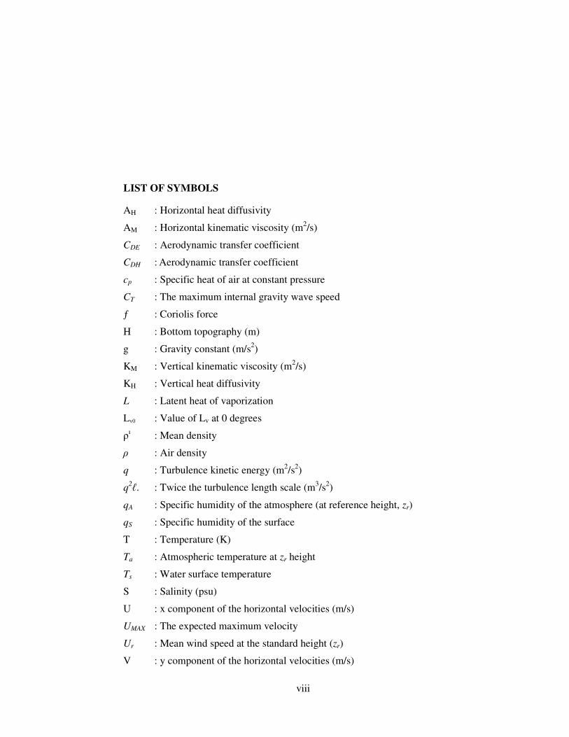
LIST OF SYMBOLS
AH : Horizontal heat diffusivity
AM : Horizontal kinematic viscosity (m2/s)
CDE : Aerodynamic transfer coefficient
CDH : Aerodynamic transfer coefficient
cp : Specific heat of air at constant pressure
CT : The maximum internal gravity wave speed
ƒ : Coriolis force
H : Bottom topography (m)
g : Gravity constant (m/s2)
KM : Vertical kinematic viscosity (m2/s)
KH : Vertical heat diffusivity
L : Latent heat of vaporization
Lv0 : Value of Lv at 0 degrees
#ı : Mean density
! : Air density
q : Turbulence kinetic energy (m2/s2)
q2". : Twice the turbulence length scale (m3/s2)
qA : Specific humidity of the atmosphere (at reference height, zr)
qS : Specific humidity of the surface
T : Temperature (K)
Ta : Atmospheric temperature at zr height
Ts : Water surface temperature
S : Salinity (psu)
U : x component of the horizontal velocities (m/s)
UMAX : The expected maximum velocity
Ur : Mean wind speed at the standard height (zr)
V : y component of the horizontal velocities (m/s)

ix
$ : Velocity component normal to sigma layer (m/s)
% : Surface elevation
& : Sigma coordinate
'XX : Friction in xx surface
'XY : Friction in xy surface

x
SUMMARY
INVESTIGATIONS OF THE HYDRODYNAMICS OF LAKE VAN USING
POM (PRINCETON OCEAN MODEL)
Large lakes are interesting dynamically because they are under the similar forcing
effect as the oceans, but it is not necessary to specify open boundary conditions in
lake because of their geometry and therefore it is easier to formulate models of their
hydrodynamics.
In this study, hydrodynamic behavior of Lake Van under a variety climatic forcings
is investigated. POM (Princeton Ocean Model) was chosen for this study because of
its wide range of usage and existence useful tools for setting up a specified problem.
POM is a three dimensional, terrain-following sigma coordinate, free surface,
primitive equation ocean model, which includes a turbulence sub-model. The model
solves principal Navier-Stokes equations.
In order to study the behavior of the model for various basin shapes and different
climatic forcings, various test cases have been examined, illustrating idealized lake
geometries such as ellipsoid, flat bottom box and inclined bottom box. Through these
test cases, it has been observed that the temperature distribution in the lake is closely
related to wind forcing applied at the lake surface. Moreover, sensible, latent and
upward longwave heat losses influence horizontal and vertical temperature
distribution and currents in the lake.
After the all of these ‘idealized geometry’ simulations, POM was run for each season
with ‘real’ lake bathymetry using long-time seasonal averages of forcing parameters.
Seasonal simulations show that lake is controlled of the climatic forcing. In summer
and winter, Lake Van is stratified and the mixing process is dominant in fall season.
The seasonal climatic forcing induces gyres in the deepest region of the lake.

xi
ÖZET
VAN GÖLÜ’ NÜN H"DROD"NAM"#"N"N POM (PRINCETON OCEAN
MODEL) YARDIMI "LE ARA$TIRILMASI
Büyük göllerin dinamik açıdan oldukça ilginçtirler çünkü okyanuslara etki eden aynı
türden kuvvetlerin etkisi altındarırlar fakat oktanuslarda oldu"u gibi göllerde açık
sınır !artlar belirlemek gerekmez ve kapalı bir ortam içinde oldukları için göller
üzerinde hidrodinamik çalı!ma yapmak daha kolaydır.
Bu çalı!mada Van Gölü’ nün iklimsel etkiler altındaki hidrodinamik davranı!ı
incelenmi!tir. Bu inceleme için geni! bir kullanım alanına ve çe!itli yardımcı
programlara sahip, POM (Princeton Ocean Model) seçilmi!tir. POM üç boyutlu,
dü!eyde topografyayı izleyen sigma kordinatı kullanan ve temel Navier-Stokes
denklemlerini çözen bir modeldir.
Öncelikle modelin farklı iklimsel etkiler altındaki davranı!ını incelemek için çe!itli
test simulasyonları yapıldı. Bu testlerde elipsoid ve kutu gibi idealize edilmi!
geometriler kullanıldı. Sonuçta göldeki sirkülasyonun ve buna ba"lı olarak sıcaklık
da"ılımının rüzgar ile büyük oranda ili!kili oldu"u bulundu. Ayrıca gizli ısı,
hissedilir ısı ve göl yüzeyinden atmosfere olan uzun dalga boylu ısı kayıplarının,
göldeki ısı da"ılımını, dü!ey ve yatayda meydana gelen hareketleri büyük ölçüde
etkiledi"i anla!ılmı!tır.
Tüm bu test simulasyonlarından sonra model herbir mevsim için ayrı ayrı mevsimsel
ortalama de"erler ile çalı!tırılmı! ve her bir mevsim kendi içinde de"erlendirilmi!tir.
Mevsimsel simulasyonlar Van Gölü’ nün büyük ölçüde iklimsel etkiler altında
oldu"unu göstermektedir. Yaz ve Kı! aylarında göl dü!ey olarak termal tabakala!mı!
bir yapıdadır. Sonbahar’ da ise karı!ım tüm gölde baskın olan durumdur. Ayrıca
mevsimsel etkiler ve rüzgar nedeniyle gölün derin olan bölgelerinde döngüsel
akıntılar olu!maktadır.

1
1. INTRODUCTION
1.1. Purpose
In the proposed project, main patterns of the surface currents, vertical circulation and
temperature profile will be considered in a seasonal context for Lake Van. On the
other hand, the main aims of this study are to understand the sensitivity
hydrodynamic properties of Lake Van as related to atmospheric ‘climate’ forcing
Moreover, in order to realize the behavior of the model to various basin shapes and
different amount of atmospheric forcing, different test cases have been considered.
1.2. Literature Review
The main subject of the hydrodynamics of lakes is the investigation of the motion of
water body (in different scales and forms) which is generated by external forces and
with their interaction (K. Hutter, 1983). Because of the complexity of the subject,
numerical models, which use fundamental physical principles, try to simulate these
motions, which can be observed in the real world.
Numerical ocean models use different assumptions and physics such as hydrostatic
equilibrium, incompressibility, free or rigid surface. It can be applied for a large
water mass as a lake and the results of the simulations are used for forecasting of the
physical structure of the large lakes (Killey et al., 1998).
Large lakes are particularly interesting dynamically because of their behavior similar
to coastal ocean and it is easier to study than the coastal ocean because they are
smaller in size, but most importantly because it is not necessary to specify open
boundary conditions (Beletsky et al. 1997). Most of the studies about hydrodynamic
modeling of lakes, examine vertical and horizontal circulations (upwelling and

2
downwelling) which are generated by wind stress (V. Botte, A. Kay, 2002; B. V
Chubarenko et al., 2001).
Dynamic and thermal structures of lake can be used for generating initial and
boundary conditions in biological models (C. Chen et al., 2002) because thermal
stratification and currents affect and organize the physical and biological process
(Ahsan et al., 1999). In addition, atmospheric heating and cooling, along with the
wind stress, determine the formation, maintenance and eventual destruction of the
surface mixing layer and control other large and small scale processes such as
circulations and internal wave generations (Ahsan et al., 1999).
Inland water or lake has a complex hydrodynamic structure and all process in
different levels (epilimnion, metalimnion and hypolimnion etc.) should be studied
separately and studying lake behaviors under thermal stratification condition (Bonnet
et al., 2000; B. R. Hodges et al., 2000; J. Heinrich et al., 1981; E. A. Tsvetova,
1999).
The application of these studies have been made for the studying, forecast of the
three-dimensional physical structure of inland water body (Kelley et al., 1998),
obtaining initial and boundary conditions for analyzing of water quality using
biochemical model (K. Taguchi, K. Nakata, 1998), understanding basin’s ecosystem
and studying three-dimensional spatial distribution of phytoplankton, dissolved
organic matter, nutrients, mineral and dissolved oxygen in lake (V. V. Manshutkin et
al., 1998).
Although, Lake Van is the largest soda lake on earth and fourth largest closed lake,
hydrological studies and available measurements about it are insufficient. In late of
70’s, hydrographical and geological properties of lake were studied by M.T.A.,
Ankara (Kempe et al., 1978). It consists of main vertical profile of temperature in
summer, chemistry analysis of lake water. and all of the studied which is related with
geology of Lake Van are collected in a book (Degens, E. T. and F. Kurtman, 1978).
Other studies are related with water level fluctuations ((en, Z. et al., 2000) and
effects of the climatic changes above it (M. Kadıo"lu et al., 1997).

3
1.3. Why is POM (Princeton Ocean Model)?
POM is a three-dimensional, sigma coordinate, free surface, primitive equation ocean
model, which includes a turbulence sub-model. The model has been used for
modeling of estuaries, coastal regions, lakes and open oceans.
POM was used in determining hydrodynamic properties of Lake Van because it has a
wide range usage. There are over 1500 POM users of record and it easy to reach and
share any knowledge using user-list. Moreover, there are more useful tools and
simple subroutines for setting up a problem and studied version of it (Pom2k) creates
NetCDF output data file and it is easy to visualization of it.

4
2. PRINCETON OCEAN MODEL (POM)
2.1. Introduction
In this chapter, it will be given some useful information about Princeton Ocean
Model (POM). The main physical principles of the model, assumptions and structure
of the code will be examined.
2.2. Description of Princeton Ocean Model (POM)
First version of The Princeton Ocean Model (POM) was developed in the late 1970's
by Blumberg and Mellor for modeling of estuaries, coastal regions and open oceans
hydrodynamic properties. Since then, it has been improved and used by most of
people all over the world so that it has several different version and type such as MPI
and HPF parallel versions of POM contributed by S. Piacsek (NRL), a non-
Boussinesq version of POM, two-dimensional version of POM etc. In this study
NetCDF output version that is called Pom2k was used for analysis. The original
version of this code named "OZPOM" which is created by John Hunter from
University of Tasmania in Australia.
POM is a three-dimensional sigma-coordinate primitive equation model with a free
surface, using a time splitting technique to solve the equation of continuity,
momentum and diffusion, using finite difference method. The external mode
(barotropic mode) of the model is two-dimensional (2D) and it uses short time step
because of computing surface elevation (high resolution). Unlike external mode,
internal mode (baroclinic mode) of the model is three-dimensional (3D) and it uses
long time step. Both of the modes (internal and external) are based on The Courant-
Frederic’s-Levy (CFL) condition.

5
The Level 2.5 Mellor-Yamada turbulence closure scheme is used for providing
realistic parameterization of vertical mixing and governing surface and bottom
boundary layers. Free surface elevation is also computed for simulating tides and
storm waves. It uses second order horizontal differencing on Arakawa C grid in
curvilinear orthogonal or rectilinear coordinates and sigma coordinate level that is a
necessary attribute in dealing with significant topographical variability, in vertical. In
sigma coordinate model vertical coordinate scaled with water column depth.
In this version, it has some case studies that should run with no additional data
requirements such as seamount and conservation box problem. Users have to write
their own code to set up specific problem or test cases which consist of initial
condition and lateral and surface boundary conditions.
2.2.1. The Basic Equations
POM is a primitive equation model and it solves main equations of fluid motion in
three-dimensional space using time splitting method. It is a terrain following sigma
coordinate model which is used in many ocean applications. In the following section,
consist of some of the principal equation and approximations which are used in
POM.
The transformation (Blumberg and Mellor, 1980) between the Cartesian coordinate
system and the sigma coordinate system can be written as,
xx =* , yy =* , ηησ
+−=
Hz , tt =* (2.1a), (2.1b), (2.1c), (2.1d)
x, y, z are the conventional Cartesian coordinates; η+≡ HD where H(x, y) is the
bottom topography and #(x, y, t) is the surface elevation. Sigma coordinate ranges
from != 0 at z= # to != -1 at z= -H.
The resulting sigma coordinate system that follows the bottom is depicted in the
following figure (Mellor, 1998),

6
Figure 2.1 the sigma coordinate system
The basic equations can be written in horizontal Cartesian coordinates,
0=∂∂+
∂∂+
∂∂+
∂∂
tyDV
xDU η
σω
(2.2)
xgDfVD
Uy
UVDx
DUt
UD∂∂+−
∂∂+
∂∂+
∂∂+
∂∂ η
σω2
xM F
UD
Kd
xD
DxgD +!"
#$%&
∂∂
∂∂=′!"
#$%&
′∂′∂
∂∂′
−∂
′∂++ ' σσσ
σρσρ
ρ σ
0
0
2(2.3)
ygDfUD
VyDV
xUVD
tVD
∂∂++
∂∂+
∂∂+
∂∂+
∂∂ η
σω2
yM F
VD
Kd
yD
DygD +!"
#$%&
∂∂
∂∂=′!
"
#$%
&′∂′∂
∂∂′
−∂
′∂++ ' σσσ
σρσρ
ρ σ
0
0
2(2.4)
zR
FT
DKT
yTVD
xTUD
tTD
TH
∂∂−+!"
#$%&
∂∂
∂∂=
∂∂+
∂∂+
∂∂+
∂∂
σσσω (2.5)
SH F
SD
KSy
SVDx
SUDt
SD +!"#
$%&
∂∂
∂∂=
∂∂+
∂∂+
∂∂+
∂∂
σσσω (2.6)

7
!"
#$%
&∂∂
∂∂=
∂∂+
∂∂+
∂∂+
∂∂
σσσω 22222 q
DKq
yDVq
xDUq
tDq q
qHM F
BDq
KgVU
DK +−
∂∂+
!!"
#
$$%
&()*
+,-
∂∂+(
)*
+,-
∂∂+
!1
3
0
22 2~22σρ
ρσσ(2.7)
!"
#$%
&∂
∂∂∂=
∂∂+
∂∂+
∂∂+
∂∂
σσσω !!!!! 22222 q
DKq
yDVq
xDUq
tDq q
!! FB
DqWKgEVUD
KE H
M +−((
)
*
++
,
-
∂∂+
!!"
#
$$%
&()*
+,-
∂∂+(
)*
+,-
∂∂+
1
3
03
22
1~~
σρ
ρσσ(2.8)
The transformation to the Cartesian vertical velocity is
ttD
yyD
Vxx
DUW
∂∂+
∂∂+((
)
*++,
-∂∂+
∂∂+(
)*
+,-
∂∂+
∂∂+= ησησησω (2.9)
$ is the velocity component normal to sigma surfaces.
The horizontal viscosity and diffusion terms are defined according to,
)()( xyxxx Hy
Hx
F ττσ∂∂+
∂∂≡ (2.10)
)()( yyxyy Hy
Hx
F ττσ∂∂+
∂∂≡ (2.11)
where
xUAMxx ∂
∂= 2τ , (()
*++,
-∂∂+
∂∂=
xV
yU
AMxyτ , yVAMyy ∂
∂= 2τ (2.12a), (2.12b), (2.12c)
Also,
)()( yx Hqy
Hqx
F∂∂+
∂∂≡φ (2.13)
xAq Hx ∂
∂= φ , y
Aq Hy ∂∂= φ (2.14a), (2.14b)

8
and " represents T, S, q2, q2". The vertical mixing coefficients for momentum KM
and heat KH, turbulent kinetic energy q2/2 and turbulent length scale ", horizontal
diffusion for momentum AM and heat AH and these are controlled with inverse,
horizontal turbulence Prandtl number.
2.2.2. Approximations
The Navier-Stokes equations for an incompressible fluid under the hypothesis of
hydrostatic equilibrium and the Boussinesq approximation are used in POM.
In the Boussinesq approximation, one suppose that density differences are small in
the sense that density variations are important in the Archimedean buoyancy force,
but not, when density arises as a factor of a rate term (K. Hutter, 1983). On the other
hand, the buoyancy drives the motion because of density varies little in which the
temperature varies little. Thus the variation in density is neglected everywhere except
in the buoyancy term.
2.2.3. Set up problem and defining constants
POM can be run for three different cases such as seamount, conservation box and
specific problem but “my_problem” subroutine can be written for it. The seamount
and conservation box subroutines are test cases for understanding how the model
works. For defining a specific problem first of all “my_problem” subroutine must be
customize. Structure of this part of the code depends on user and there are no strict
rules about that but users must define some constants and construct their physical
environment, boundary and initial conditions of the problem by code.
First of all it is necessary to define grid type and grid points coordinates. POM can be
run both curvilinear orthogonal and rectilinear coordinates with “Arakawa C”
differencing scheme. After choosing horizontal grid type, grid points coordinates can
be calculate.
Fig. 2.2 and 2.3 represent internal and external grid structures of the model. Potential
temperature, salinity, density and horizontal velocities are calculated in the middle of
the sigma layers and vertical velocity and turbulence energy are estimated in each
sigma layer in three dimensional internal mode.

9
Figure 2.2 The three-dimensional internal mode grid structure (Q represents KM, KH, Q2, Q2L and T represents T, S and RHO)
Figure 2.3 The two-dimensional external mode grid
There are some useful subroutine and program for pre-processing such as generating
grid points and objective analysis but users have to be able to create your own pre-
processing code for implementing their special problem into model.
After calculating coordinates of grid points and interpolating of the bathymetry data
into cell center of the grid, land and sea masking must be apply. It must be more
attention to masking process because land is set in POM as H=1 instead of 0 to allow
division by H. There are three different masking variables (FSM, DUM and DVM);
DUM is masking for u component of velocity, DVM, masking for v component of
velocity and FSM masking for scalar variables. All of them must be set to 0 over
land and 1 over water.

10
Initial and boundary conditions must be set in next step. If it is necessary to create
setting time dependent, surface and lateral boundary conditions (such as wind stress,
temperature and salinity flux etc.), this designation must be in beginning of the
internal three-dimensional mode. This part of the code begins with a loop which is
labeled with 9000.
It is necessary to notice during applying forcing component of the model;
Wind stress; stress and wind direction are opposite and eastward and northward
winds stress have negative signs, eastward and northward currents have positive
signs. On the other hand, if the wind is blowing from east to west or north to south,
wind stress must be negative sign.
Flux components; sensible, latent heat (which involves only the evaporative
component) and long wave radiation are defined as one value. The heat flux is
positive when the water is cooling and negative when the water is warming. Latent
heat and sensible heat can be calculated in Wm-2 unit using following formula for
defining time dependent boundary condition.
))(( rasrDHp zTTUCcSH −= ρ (2.15)
))(( rasrDE zqqUCLLH −= ρ (2.16)
TLL vo 2369−= (2.17)
where, cp is the specific heat of air at constant pressure, ! is air density, L is the latent
heat of vaporization (can be calculated using Eq.2.17, where Lv0 is the value of Lv at
0 degrees C, taken as 2500297.8 Jkg-1, and T is the temperature in Celsius), Ur is
mean wind speed at the standard height (zr), Ts is water surface temperature, Ta is
atmospheric temperature at zr height, qa and qs are specific humidity of the surface
and atmosphere (at reference height, zr), CDE and CDH are aerodynamic transfer
coefficients. If the wind speed at 10 m is 5 ms-1, CD=3.10-3.
Constants, coefficients, parameters, mode and scheme are defined in beginning of the
model. It is possible to select three different calculation types and it affects
calculation of the bottom stress and 3D calculation can be made as prognostic and
diagnostic.

11
It can be used two different advection scheme (centered and Smolarkiewicz iterative
upstream scheme) but changing iteration step for Smolarkiewicz scheme is caused to
more CPU time.
Jerlov water type controls how the ocean volume scatters light. Type I waters were
represented by extremely clear oceanic waters. However, many water bodies were
found to lie between Types I and II and the former was subsequently split into Types
IA and IB. Type III waters are fairly turbid and some regions of coastal upwelling
are so turbid that they are unclassified. To specify the penetration of short wave
radiation, this classification is used.
External and internal time steps are related with grid size and maximum magnitude
of velocity,
21
22
111−
+≤∆yxC
tt
E δδ (2.18)
max2/1)(2 UgHCt += (2.19)
21
22
111−
+≤∆yxC
tT
I δδ (2.20)
max2 UCCT += (2.21)
where H is the depth of the location, UMAX is the expected maximum velocity in
Eq.2.18 and 2.19. According to this relationship between external time step and
depth, as the depth increases the internal time step also decreases. In Eq.2.20, CT is
the maximum internal gravity wave speed and UMAX is the maximum advective wave
speed (Eq.2.21). The internal and external time steps are connected with a ratio of
time step (“ISPLIT” variable in program) and typical value of the ratio is 30 for
coastal ocean conditions.
Using value of grid size and velocity, CFL (The Courant-Fredrics-Levy) condition
are calculated each loop (internal three-dimensional mode, labeled as 9000). If
velocity is higher than defined constant value of maximum velocity, code stops
because of the CFL condition and it gives “abnormal job and user terminated” error.
For avoiding this error, time steps must be decrease or grid size must be increase.

12
Internal value of horizontal kinematic viscosity and heat diffusivity (“AAM”
parameter in POM) coefficients can also cause “abnormal job and user terminated”
error. Horizontal kinematic viscosity and heat diffusivity are connected each other
with inverse horizontal turbulent Prandtl number (“TPRNI” parameter) and heat
diffusivity affect the flux of heat from the surface to the bottom of lake. If the value
of “AAM” is greater than a critical value, error occurs. “AAM” depends on grid size
and velocity gradients. The diffusion component dominates the advection component
in great kinematic viscosity value and error which is created by advective terms
could be reduced. The grid cell Peclet number or cell Reynolds number can be used
for calculating initial kinematic viscosity value. Small cell Reynolds number means
it is diffusion dominated environment. Otherwise, large cell Reynolds number means
it is advection dominated space.
Inverse horizontal turbulent Prandtl number is defined as dimensionless ratio
between horizontal thermal diffusivities and horizontal momentum eddy viscosities
and the typical value of it 0.2 but there are some test case application which it is
assumed to be 1.0 (Beletsky et al., 1997).
It can be given specific data file for a seamless restart. This data had been crated by a
previous run of the POM.
2.2.4. Structure of main program
After defining the problem and its initial, boundary conditions, the program begins to
forecast variables. To compute baroclinic pressure gradient, density must be
calculated by equation of state UNESCO (Mellor, G. L., 1991).
POM uses a mode-splitting technique to solving internal and external variables;
external mode solves surface elevation and vertically time average wave speed to
using in the internal mode and it uses density and vertically means velocity that is
created by internal mode for calculating surface elevation. Subroutine ADVAVE also
calculates the bottom stress in external mode and boundary conditions and velocity is
defined by using subroutine BCOND.
Internal step compute three-dimensional variables that are separated into a vertical
diffusion time step and an advection plus horizontal diffusion time step. It solves
fully three-dimensional temperature, turbulence and current structure.

13
Advection part of the internal mode is solved by subroutine ADVT and vertical
diffusion part is solved by subroutine PROFT. Both of them are calculated for
temperature and salinity.
!"#$%& '()%*+%,$#)#"-%./$0#)#/$1
2345%)6")%-")(7"-%)6(78/09$"8#.%:/*$0"79%./$0#)#/$1%"7(%/;)($%1()%(<*"-)/%)6(%#$#)#"-%./$0#)#/$1%"$0%"7(%6(-0%./$1)"$)%)6(7(";)(7=%>1(71%."$%/;./*71(%.7(")(%?"7":-(%:/*$0"79%./$0#)#/$1=
!"#$%"&'()*+)(,
!"#$%"&'()*#-$%./
"-.*-")(1%%:"7/.-#$#.+7(11*7(%!7"0#($)="#%"$0%9%./8+/$($)$
!"#$%"&'()*.$01
!"#$%"&'()*.$012
!"#$%"&'()*.$02
!"#$%"&'()*.$12
!"#$%"&'()*.$'(&-33
!"#$%"&'()*4'(+.,'
"-.*-")(1%)6(1)7("8%;*$.)#/$%%+7#$)1%1)7("8;*$.)#/$%*&?
$().0;';#-(%()*$/$().0;*
47*(!"#$%"&'()*
5$'&)6()&7+489::;<=>89
!/0(%()%+,,2345%+
-"-1(
!"#$%"&'()*-+?7&47*(
"-.*-")(1%)6(%6/7#./$)"-+/7)#/$1%/;%8/8($)*8
!"#$%"&'()*#-$%./
!"#$%"&'()*-+?-?)
"-.*-")(1%6/7#./$)"-"0?(.)#/$%"$0%0#;;*1#/$
!"#$%"&'()*#7%(+8 9!::;<=>8"
8/0"#(#)+"0?$/0%,,2345%1
!"#$%"&'()*-+?-?)47*(
!"#$%"&'()*#7%(+8 #!::;<=>8"
-"-1(
-"-1(
;<=>!*
9$8/+)#/$%&=%)/%#$#)#"-#.(%;#-(&%+=%)/%27#)(%"%1()%/;%0")"&%3=%)/.-/1(%;#-(
#$ !/0(%+&%345%."-.*-")#/$%":/))/8%1)7(11%."-.*-")(0%#$+7/;*&?$
%$8#1+-#)%"#1+-#)/#$)(7$"-%35%)#8(%1)(+%6%(#)(7$"-%+5%)#8(1)(+$
"$87++-#(1%/+($%:/*$0"79%./$0#)#/$18%"/+)#/$1$%%%%&44%5#)(7$"-%"+45$%:/*$0"79%./$0#)#/$1%%%%+44%5#)(7$"-%"+45$%?(-/.#)9%%%%344%,$)(7$"-%"345$%:/*$0"79%./$0#)#/$1%%%%944%4(8+(7")*7(%%%'"-#$#)9%:/*$0"79%./$0#)#/$1%%%%144%:(7)#."-%?(-/.#)9%:/*$0"79%./$0#)#/$1%%%%;44%<+%")2#.(%)6(%)*7:*-($.(%<#$()#.%($(7!9$%%%<+-%"<+%,%%%%%%%%%)*7:*-($.(%-($!)6%1."-($
&$8#1+"0?&%')(+%#$)(7?"-%0*7#$!%26#.6%(#)(7$"-%"+45$8/0(%"0?(.)#?(%)(781%"7(%$/)%*+0")(0%"0#8($1#/$-(11$
'-'(8#
=("0%5")"
$7("0%/%&
47*(
$7("0/&%8("$1%)6")0")"%6"0%:(($%.7(")(0:9%"%+7(?#/*1%7*$ -"-1(
!"#$%"&'()*.$01
8/0(%()%+
!"#$%"&'()*.$0128::
47*(
!"#$%"&'()*.$028::
!"#$%"&'()*.$128::
-"-1(
()/'(8'(&)$(-38 %)*!+%+)
,---8..;=8/8908.>;*
()/'(8)0&)$(-38 #)*!+%+)
1---8.>2=8/8908.!34.=::;<=>8%
5-37"3-&'(/8!"$4-7)>3)?-&'%(8 >4!
47*(>(+8%48)0&)$(-38 #)*!+%+)1---
"-.*-")(1%0($1#)9%*1#$!>25' 3%(<*")#/$%/;1)")(%"1"-#$#)9&%+/)($)#"-)(8+=&+7(11*7($
>7#)(1%"%6/7#./$)"-%+45;#(-0=%?7#0%#$.7(8($)&(-(?")#/$%+/#$)1&*$0#1)*7:(0%2")(7%0(+)6().=
>7#)(1%6/7#./$)"-%-"9(71/;%"%345%;#(-0%2#)6#$)(!(71%/7%;-/")#$!%+/#$)$*8:(71="@/7#./$)"--94"?(7"!(00($1#)9$
>7#)(1%?(7)#."-%1(.)#/$%/;%"%345;#(-0&%#$%)6(%#4%/7%#40#7(.)#/$="@/7#./$)"--94"?(7"!(0%0($1#)9$
>7#)(1%?(7)#."-%1(.)#/$%/;%"%345;#(-0&%#$%)6(%94%/7%A40#7(.)#/$="@/7#./$)"--94"?(7"!(0%0($1#)9$
B7#$)1%0(+)64"?(7"!(0%*%"$0%?&1*7;".(%(-(?")#/$)/%/*)+*)%0(?#.(%;
,,%*&%?&%2&%+/)($)#"-)(8+(7")*7(&1"-#$#)9&%)*7:*-($)<#$()#.%($(7!9%,+&)*7:*-($)%-($!)61."-(&%6/7#./$)"-"$0%?(7)#."-<#$(8")#.%?#1./1#)9"$0%0#;;*1#?#)9
!6%$&85-?)8$-+'-&'%(083%(/85-?)8$-+'-&'%(08,)(,'#3)86)-&8-(+83-&)(&86)-&8/8-$-8-(+87-37"3-&)8,+-/%$'(,7183-&)$-38?',7%,'&1
"-.*-")(16/7#./$)"-"0?(.)#/$%"$00#;;*1#/$=
!"#$%"&'()*5$'&)6()&7+48#
::;<=>893%+#7$( ()&7+4!
Figure 2.4 Structure of the main program (Part 1)
Beginning of the internal mode, POM calculates Smagorinsky lateral viscosity and
the vertical averages of three-dimensional variables for using in two-dimensional
external mode and two-dimensional external mode and all time dependent surface
and lateral boundary conditions are set up in this section of model. Wind stress, heat
and salinity fluxes are defined in this part of the code. External mode calculations

14
results in updates for surface elevation and vertically averaged velocities. The
internal mode calculation results in updates for velocity components (U and V),
temperature and salinity.
'-'(8# :7!7C%(/:!7CD
47*(
-"-1(
!"#$%"&'()*?)$&?3
::;<=>89
!"#$%"&'()*#7%(+ &!::;<=>8#
!"#$%"&'()*.$%48
::;<=>8"
!"#$%"&'()*#7%(+ 9!::;<=>8#
!"#$%"&'()*-+?8 :#!::;<=>8%
!"#$%"&'()*-+?8 :#4!::;<=>8%
23458
9$8 "-.*-")(1%?(7)#."-%?(-/.#)9
#$87++-#(1%/+($%:/*$0"79%./$0#)#/$18%"/+)#/$1$%%%%&44%5#)(7$"-%"+45$%:/*$0"79%./$0#)#/$1%%%%+44%5#)(7$"-%"+45$%?(-/.#)9%%%%344%,$)(7$"-%"345$%:/*$0"79%./$0#)#/$1%%%%944%4(8+(7")*7(%%%'"-#$#)9%:/*$0"79%./$0#)#/$1%%%%144%:(7)#."-%?(-/.#)9%:/*$0"79%./$0#)#/$1%%%%;44%<+%")2#.(%)6(%)*7:*-($.(%<#$()#.%($(7!9$%%%<+-%"<+%,%)*7:*-($.(%-($!)6%1."-($
%$8 "-.*-")(1%6/7#./$)"-%"0?(.)#/$%"$0%0#;;*1#/$&%"$0%?(7)#."-%"0?(.)#/$%;/7%)*7:*-($)<*"$)#)#(1=%")6(%"0?(.)#?(%)(781%;/7%)6(%)*7:*-($.(%<*"$)#)#(1$
"$8'/-?(1%;/7%<+%")2#.(%)6(%)*7:*-($)%<#$()#.%($(7!9$&%<+-%"<+%#%)*7:*-($)%-($!)61."-($&%<8%"?(7)#."-%<#$(8")#.%?#1./1#)9$%"$0%<6%"?(7)#."-%<#$(8")#.%0#;;*1#?#)9$&%*1#$!"%1#8+-#;#(0%?(71#/$%/;%)6(%-(?(-%+%&6+%8/0(-%/;%!(--/7%"$0%E"8"0"%"&FG+$=
&$8 "-.*-")(1%H/)6%)(8+(7")*7(%"$0%1"-#$#)9=%-/7%"0?)+&%7(0*.(1%#8+-#.#)%0#;;*1#/$*1#$!%)6(%'8/-"7<#(2#..%#)(7")#?(%*+1)7("8%1.6(8(%2#)6%"$%"$)#0#;;*1#?(%?(-/.#)9=
9$827#)('$().0;%/+)#/$&%&%)/%#$#)#"-#1(%;#-(&%+%)/%27#)(%"%1()%/;%0")"&%3%)/%.-/1(%;#-(
!/0(%()%9
70?(.)#/$%1.6(8($"0?%/&
47*(
!"#$%"&'()*-+?&9
::;<=>8&
47*(
!"#$%"&'()*-+?&#
::;<=>8&
-"-1( 70?(.)#/$%1.6(8($"0?%/+
47*(
-"-1( >0'&3$%/$-+
!"#$%"&'()*.$%4& =!
!"#$%"&'()*.$%4& !!
!"#$%"&'()*#7%(+ "!
!"#$%"&'()*+)(,
!"#$%"&'()*-+?"-"-1(
!"#$%"&'()*-+??
!"#$%"&'()*.$%4"
!"#$%"&'()*.$%4?
!"#$%"&'()*#7%(+ %!
>(+8%48&6)8'(&)$(-38 %)*!+%+),---
>;*8<;=<>83<' ;>=5*;=>>!.<;!
,$)(!7")(1./$1(7?")#?(1."-"7(<*")#/$1= 524=55' @5!7
,$)(!7")(1./$1(7?")#?(%1."-"7(<*")#/$1=%-,='443=55=>B'4=57!' @5!5
'/-?(1%;/7%?(7)#."-0#;;*1#/$%/;%)(8+(7")*7("$0%1"-#$#)9%*1#$!%8()6/00(1.7#:(0%:9%=#.68(9(7"$0%!/7)/$=
5/(1%6/7#./$)"-%"$0?(7)#."-%"0?(.)#/$%/;%*48/8($)*8&%"$0%#$.-*0(1./7#/-#1&%1*7;".(%1-/+(%"$0:"7/.-#$#.%)(781=
5/(1%6/7#./$)"-%"$0?(7)#."-%"0?(.)#/$%/;%?48/8($)*8&%"$0%#$.-*0(1./7#/-#1&%1*7;".(%1-/+(%"$0:"7/.-#$#.%)(781=
'/-?(1%;/7%?(7)#."-0#;;*1#/$%/;%#48/8($)*8*1#$!%8()6/0%0(1.7#:(0:9%=#.68(9(7%"$0!/7)/$=
'/-?(1%;/7%?(7)#."-0#;;*1#/$%/;%948/8($)*8*1#$!%8()6/0%0(1.7#:(0:9%=#.68(9(7%"$0!/7)/$=
$().0;';#-(%()*$/$().0;*
3%+#7$( ()&7+4!
!"#$%"&'()*5$'&)6()&7+48#
::;<=>8947*(
-"-1(
!"#$%"&'()*.$'(&-33
!"#$%"&'()*5$'&)6()&7+48%
::;<=>89
"-.*-")(1%)6(%"$)#0#;;*1#?(?(-/.#)9%*1(0%)/%7(0*.(%)6($*8(7#."-%0#;;*1#/$"11/.#")(0%2#)6%)6(*+1)7("8%0#;;(7($.#$!1.6(8(=
!"#$%"&'()*,+%36-+'4
Figure 2.5 Structure of the main program (Part 2)
After finishing two-dimensional external loop (labeled with 8000), using external
mode calculations, sigma coordinate vertical velocity, vertical temperature and
salinity, turbulence kinetic energy and scale is calculated (see Eq.2.5, 2.6, 2.7, 2.8
and 2.9). Figure 2.4 and 2.5 is the flow chart which is represents both internal and
external mode and process in the program.

15
2.2.5. Input and Output of Model
Used version of POM creates a NetCDF file to analysis of data. NetCDF (network
Common Data Form) is an interface for array-oriented data access and it is a
collection of software libraries for C, FORTRAN, C++, Java, and PERL. The
NetCDF libraries define a machine independent format for representing scientific
data.
NetCDF data is self-describing because it consists of information about the data it
contains, Architecture-independent because it can be accessed by computers with
different ways of storing integers, characters and floating-point numbers, Direct-
access because of accessing efficiently small subset of large dataset, without first
reading through all preceding data and Sharable so one writer and multiple readers
may simultaneously access the same NetCDF file.
2.3. Possible Error Sources in POM
POM uses sigma coordinate in vertical which is used in both atmospheric and
oceanic numerical models because of the following bottom or surface topography.
The main advantage of the sigma coordinate is that a smooth representation of the
bottom topography in ocean models. Nevertheless sigma coordinate has some
disadvantage such as pressure gradient error.
Models which use terrain following coordinates, have suffered from errors in the
horizontal component of the pressure gradient over step topography. It takes large,
comparable in magnitude and opposite in sign value near step topography. In fact
that it causes only computational error in velocity and can be detected in the case of
an initially horizontally homogeneous density filed that, in theory, should produces
zero velocity (Mellor et al., 1998).
It is defined as a problem of “hydrostatic consistency” associated with the sigma
coordinate system. If a finite difference scheme to be hydrostatically consistent, it
would supply following condition,
δσδσ <∂∂
xxD
D (2.22)

16
It is known that this error is reduced by subtracting the area averaged density before
evaluating density gradients (Mellor et al., 2000). The results show that if the finite
difference schema satisfies the condition for hydrostatic consistency (Eq.2.22), the
error can be reduced to tolerable levels with sufficiently high resolution (Haney R.
L., 1991) and also greater kinematic viscosity values can be reduced error terms.
Step topography has an important role in ocean modeling. The reducing error studies
are separate into four main categories (detailed information see, Song Y. T., 1998),
Vertical Interpolation Method; in this method, sigma coordinates are converted into z
coordinate before calculating pressure gradient force terms but special care is
necessary for reducing error. Extrapolation often required and if the interpolation is
required each time step; it would be very costly in computational meaning.
Subtract reference state; this technique is formulating pressure gradient force as
derivation of a chosen reference state. It is easy to implant to the model but it is
insufficient for large modeling studies and long-term integration of it may not be
small.
Higher order method; Using high order scheme can be reduce numerical error in
computation of pressure gradient force but this approach fails to achieve significant
improvement in some cases and it may need more computational time.
Retaining integral properties; it is based on the following formula,
xhp
hxp
xp
z ∂∂
∂∂−
∂∂=(
)*
∂∂
σσ
(2.23)

17
3. STUDY AREA AND DATA
3.1. Introduction
Lake Van is situated on eastern Anatolia in Turkey at about 43°E longitude and 38.5
°N latitude and its elevation is 1648 m (Figure 3.1).
Figure 3.1 Location Map of Lake Van in Mercator projection
It has a surface area of 3574 km2, volume of 607 km3 and maximum recorded depth
in the lake is 451m (Wong et al., 1978). The lake basin is separated into two parts by
the Erek and Eastern Fans. Deveboynu Basin (surface area 11 km2) which is
elongated north-south direction and its average depth is 430 m. Tatvan Basin is much

18
larger than Deveboynu Basin (surface area 440 km2) and its average depth is 445 m
(Wong et al., 1978).
It is a closed lake which loses their water by evaporation only. Closed lakes with
morphology of rift lakes are comparatively seldom (Kempe et al. 1978).
The hydrological features have similarities with the open oceans, in winter arctic
downwelling occurs, in summer an equatorial warm surface layer is formed, and in
autumn or early winter upwelling encountered in the lake (Kempe et al. 1978).
3.2. Origin of Lake Van
Lake Van is the product of an extensive volcanic eruption of the Nemrut volcanic
mountain during the Late Pleistocene (Blumenthal et al. 1964). Lake is surrounded
by mountains and hills such as in the southwest Nemrut and Süphan, is located in the
north of the lake and its level rose rapidly with northeast-southwest fluvial system
was dammed (Kad!o"lu et al., 1987).
3.3. Climate of Region
Lake Van is located in about 43°E longitude and 38.5 °N latitude and its elevation is
1648 m. In this latitude winter is very severe and during this time mean temperature
is generally under 0 °C. The coldest month of the region is January at -6.2 °C and all
stations average of temperature is -4.79 °C in winter. Temperature reaches its
maximum value between July and September (around 20 °C) and late of the
September it starts to decrease but annual average of the temperature is above the 8
°C.
It is clear that precipitation is the highest value in April and May. In winter normally
falls as snow and in late spring there is a rainy season. Summer time is the warmest
and driest months but precipitation begin to increase with autumn as temperature
decrease. The annual average of the precipitation is 492.64 mm. Runoff is the
maximum value in May because of snow melt and heavy rain (Kadio"lu et al., 1997).
As a result of the seasonal variation of the atmospheric conditions (precipitation,
temperature etc.) and river discharge, lake level rises from January to June and falls
during the rest of the year. Maximum rise in lake level is from April to May and the
strongest decrease occurs between September and October (Kempe et al., 1978).
19
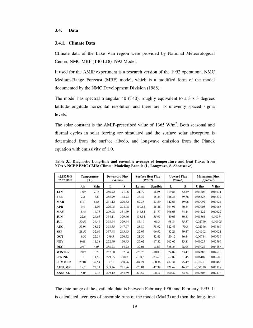
3.4. Data
3.4.1. Climate Data
Climate data of the Lake Van region were provided by National Meteorological
Center, NMC MRF (T40 L18) 1992 Model.
It used for the AMIP experiment is a research version of the 1992 operational NMC
Medium-Range Forecast (MRF) model, which is a modified form of the model
documented by the NMC Development Division (1988).
The model has spectral triangular 40 (T40), roughly equivalent to a 3 x 3 degrees
latitude-longitude horizontal resolution and there are 18 unevenly spaced sigma
levels.
The solar constant is the AMIP-prescribed value of 1365 W/m2. Both seasonal and
diurnal cycles in solar forcing are simulated and the surface solar absorption is
determined from the surface albedo, and longwave emission from the Planck
equation with emissivity of 1.0.
Table 3.1 Diagnostic Long-time and ensemble average of temperature and heat fluxes from NOAA NCEP EMC CMB: Climate Modeling Branch (L, Longwave, S, Shortwave)
42.18750 E 37.67308 N
Temperature (°C)
Downward Flux (W/m2)
Surface Heat Flux (W/m2)
Upward Flux (W/m2)
Momentum Flux (dyn/cm2)
Air Skin L S Latent Sensible L S U flux V flux
JAN 1,09 2,18 256,72 121,06 -21,79 -8,79 319,86 32,59 0,04606 0,04931
FEB 2,2 3,6 255,79 162,73 -36,47 -15,24 326,36 39,76 0,05528 0,04337
MAR 5,17 6,88 261,12 226,32 -67,38 -23,59 342,66 49,06 0,07092 0,03924
APR 9,4 11,06 276,05 294,08 -110,68 -25,46 364,91 60,84 0,07905 0,03068
MAY 15,44 16,75 299,98 351,69 -146,84 -21,77 396,05 74,44 0,04222 0,00822
JUN 22,6 24,65 334,11 379,46 -138,54 -35,93 440,65 80,81 0,01364 -0,00374
JUL 30,59 34,44 368,64 379,44 -85,19 -66,3 498,84 75,37 -0,02749 -0,00105
AUG 33,94 38,52 368,55 347,97 -28,89 -78,92 522,45 70,3 -0,02366 0,01869
SEP 28,56 32,66 337,98 293,93 -22,05 -66,92 482,29 59,47 -0,01302 0,00021
OCT 19,36 22,39 299,3 220,72 -21,36 -42,43 420,12 46,44 -0,00714 0,00736
NOV 9,68 11,38 272,49 150,93 -25,62 -17,82 362,65 33,81 0,01027 0,02596
DEC 2,97 4,08 258,73 114,72 -22,01 -8,45 328,24 28,05 0,03022 0,04286
WINTER 2,09 3,29 257,08 132,84 -26,76 -10,83 324,82 33,47 0,04385 0,04518
SPRING 10 11,56 279,05 290,7 -108,3 -23,61 367,87 61,45 0,06407 0,02605
SUMMER 29,04 32,54 357,1 368,96 -84,21 -60,38 487,31 75,49 -0,01251 0,00463
AUTUMN 19,2 22,14 303,26 221,86 -23,01 -42,39 421,69 46,57 -0,00330 0,01118
ANNUAL 15,08 17,38 299,12 253,59 -60,57 -34,3 400,42 54,24 0,02303 0,02176
The date range of the available data is between February 1950 and February 1995. It
is calculated averages of ensemble runs of the model (M=13) and then the long-time

20
average was calculated all of the variables in 42.18750 E, 37.67308 N location.
Monthly, seasonal and annual long-time average of the variables can be seen in
Table 3.1 and Fig.3.2 shows that yearly cycle of the used variables. ULW, Upward
Longwave Flux, USW, Upward Shortwave Flux, DLW, Downward Longwave Flux
and DSW, Downward Shortwave Flux. Net longwave flux is the difference between
downward and upward longwave flux.
Figure 3.2 T40 Diagnostic Long-time averages of monthly heat fluxes in Longitude, 42.1875 E and Latitude, 37.67308 N from NOAA NCEP EMC CMB: Climate Modeling Branch
3.4.2. Bathymetry Data
Bathymetry data of the Lake Van were digitized using various GIS program
(ArcView and ER Mapper) from Lake Van map which is published by Turkish Navy
Department of Navigation, Hydrography and Oceanography in 1983 (No: 9008).
The bathymetries were modified in order not to exceed hydrostatic consistency
criterion for sigma coordinates. In Chapter 5, it is given detailed information about
hydrostatic consistency.

21
4. GRID GENERATION PROGRAMS
4.1. Introduction
There is various kind of grid generation program for POM. In the oceanic modeling
applications are preferred to use boundary fitted curvilinear orthogonal grid because
of reducing computational error and increasing stability. In this section, it is given
some useful information about grid generation programs which can be used in
modeling with POM and then “LAKEGRID” grid generation program which is
written for lake studies, will be introduced.
4.2. Curvilinear Orthogonal Grid Generation Programs
“CURVIGRID.F” generates grid using four edges of the girded domain in latitude
and longitude values and it can be altered to rectilinear coordinates by setting CS
parameter to 1. It uses orthogonality conditions in Eq.4.1 and 4.2.
ij sy
sx
()*
+,-
∂∂−=(
)*
+,-
∂∂
, ij s
xsy
()*
+,-
∂∂−=(
)*
+,-
∂∂
(4.1), (4.2)
“GRID.F” uses similar technique with “CURVIGRID.F” but it can be plotted
interpolated data using NCAR Graphics routines or MATLAB m file.
Lastly, there is another grid generation program which is working under MATLAB.
It is a MATLAB toolbox which is called as “SEAGRID”. It is written by Dr. Charles
R. Denham.

22
4.3. LAKEGRID Grid Generation Program
4.3.1. Introduction
POM has an ability to use both curvilinear orthogonal coordinates and simple
rectangular Cartesian grid but if the boundary of the study area very indented (it has
a lot of convex and concave part), available curvilinear orthogonal grid generation
programs are insufficient for generating grid.
“LAKEGRID” was written in FORTRAN 95 and it is ability to produce rectangular
Cartesian grid for some simple test case such as quadrangle, circular and ellipsoid
but in this study it is used for creating grid and masking in flat bottom box, inclined
bottom box, ellipsoid test cases and real lake. Also, it uses sigma coordinates in
vertical.
It is taken advantage of some other grid generation programs such as “GRID.F” in
POM ftp site. It was written by John Wilkin of Woods Hole Oceanographic
Institution and has been changed and extended by George Mellor and Tal Ezer from
Princeton University. “PNPOLY” subroutine is written by Randolph Franklin,
University of Ottawa.
4.3.2. Input and Output Files
For generating grid of real lake case, two ASCII file must be given to program as
input file. One of them is “CONTOUR.XYZ” which is consist of two column in
degree unit (Longitude, Latitude) and other is “BATHYMETRY.XYZ” file that has
three column, first two data column are same as “CONTOUR.XYZ” and next column
is bathymetry data in meter unit and depths must be positive values.
It is not necessary to give any file to generating grid for the test cases. Program
creates boundary and bathymetry data itself.
The program creates two ASCII file which is used in POM “my_problem”
subroutine. “POMGRID.TXT” is consist of following variables of the grid points;
depth (H), masking variables (FSM, DUM and DVM), area of the cell T, U and V
(ART, ARU and ARV), Coriolis value (COR), rotation, x and y coordinates of the grid
cell (C, E, U and V) and grid spacing for each cell. Other file, “POMSIGMA.TXT”
consists of sigma level data such as sigma level thickness, coordinates of the center
of sigma levels etc.

23
4.3.3. Definition of the Subroutines
“DIST” function calculates distance between two points in meter unit. Point data
must be geographic coordinates in degree unit. This function is adapted from
SEAGRID MATLAB toolbox which is created by Dr. Charles R. Denham, U.S.
Geological Survey. Also, “DIST” is used for calculating average distance between
bathymetry observation points which is used in “CRESSMAN”.
“CELLCOOR” subroutine calculates coordinates of the grid points U, V, E and C. It
is adapted from POM2K test cases.
“CRESSMAN” subroutine interpolates scattered data into grid points using Cressman
method which is created by George P. Cressman in 1959. In this method, the
residuals are weighted depending only upon the distance between the grid point and
the observation. “DIST” is used for defining the radius of influence. If the depth is
less than minimum depth which is specified in parameter section, value of real depth
is changed to minimum depth.
“DEPTH” subroutine adapted from GRID.F program. It calculates sigma levels
coordinates and thicknesses.
“MASK” subroutine apply sea and land masking to grid cell. It uses depth data, if
depth equal to 1, it assumes land and if depth grater than 1, it is water. POM assumes
that land is 1 meter depth to insure division by H. It is also calculates cell area and
Coriolis value of each cell.
“PNPOLY” subroutine is the main part of the code. It determines whether a point is
inside or outside a boundary area. The result is used for calculating bathymetry and
applying masking. A vertical line is drawn through the point and if it crosses the
polygon an odd number of times, the point is inside of the polygon. This is called the
Jordan Curve Theorem.
“SLPMIN” subroutine is used for smoothing topography in order to insure
hydrostatic inconsistency and pressure gradient force errors.
“ZTOSIG” subroutine converts z levels to sigma levels. Vertical sigma levels can be
depth of the levels. This data preserve in ZS variable.

24
4.3.4. Program Structure
MOD, BMODE, CMODE and SMODE parameters control running styles of the
program in the beginning. Different combinations of the mode variables supply
various kind of test case and even real lake boundary with constant depth. After
definitions of the parameters and coefficients, it creates boundary data for test cases
and read boundary data of the real lake (if real lake case chosen).
It finds maximum and minimum value of grid quadrant which contains all of the
boundary vertexes and it calculates grid count in x and y direction for defining
dimensions of the arrays.
After finding dimension of the arrays, coordinates of the grid points are calculates
using “CELLCOOR” subroutine. Next step is defining grid points whether a point is
inside or outside a boundary area using “PNPOLY” subroutine.
The depth is designated as land in all points which is the outside of the boundary area
and created (for test cases only) or read bathymetry data interpolated in to center of
the grid pointes using “DIST” function and “CRESSMAN” subroutine.
The land and water masking are calculated using result of the “PNPOLY” subroutine
and than using result of the “PNPOLY” both depth data and sigma levels are
computed. After computing masking variables, bathymetry data are smoothed using
“SLPMIN” subroutine.
Time step for each cell and hydrostatic inconsistency factor on bottom layer (should
be less than 1 for stability) are calculated and controlled.

25
5. APPLICATIONS OF THE MODEL
5.1. Simple Test Cases
In order to how the model works and gives response to different amount of forcing, it
is examined for various lake shape, bathymetries, wind and heat flux forcing. Three
main basin types are used in test cases which are called ellipsoid (EL), flat bottom
box (BC) and inclined bottom box (BI). EL and BI basin shape and bathymetries can
be seen in Figure 5.1 and 5.2. All of the basins have same surface area of 3600 km2
which is equal to Lake Van's.
Every one of the test case simulations has same initial temperature distribution in
vertical and horizontal scale and it is assumed that the lake is isothermal and not
stratified. Annual average temperature of Lake Van is used to setting up initial
conditions of test cases, so both atmospheric temperature (TATM) and vertical
temperature distributions of lake are constant in 9 °C.
At the beginning of the all test case simulations, there is no motion in the lake and
free surface is initially flat. The lateral boundary conditions are no-slip namely
tangential and normal components of the velocity set to zero at the lake boundary.
The Lake Van centered at latitude 38.5 N. so that the Coriolis parameter is assumed
to be constant at f =10-4 s-1. A rectangular horizontal grid with a uniform spacing
()x=)y) of 1 km was used and 20 vertical sigma levels were used with closer
spacing near the surface at z= 0, 1, 2, 3, 5, 8, 12, 18, 25, 35, 50, 70, 100, 125, 150,
175, 200, 225, 250 and 300 m.
Horizontal diffusion is calculated with Smagorinsky eddy parameterization
(HORCON parameter is 0.1); horizontal momentum diffusion is assumed to be equal
to horizontal thermal diffusion (Inverse horizontal turbulent Prandtl number is 1.0).

26
For test case reference density is set to a constant value 1020 kg/m3 and salinity is
constant in 20 psu which is same as Lake Van. To insure computational stability,
POM uses an internal mode time step of 180 s and external mode time steps of 6 s
for the 1 km grid.
The wind stress increases linearly from zero to its maximum value over 24 hours and
it remains constant at this maximum value for the duration of the model simulation.
It is used two different wind speed for simulating strong wind (5 m/s) and light wind
cases (1 m/s) and Table 5.1 is represented wind speed and its stress equivalents.
Table 5.1 Applied Wind Stress in test cases
Wind Direction m/s N/m2 m2/s2
N-S and E-W 1.0 0.00125 0.00125 ×10⁻³
5.0 0.031 0.031 ×10⁻³
NE-SW (5 m/s) x and y component 2.236 0.006 0.006 ×10⁻³
The net solar radiation at the ground peaks near local solar noon (Hartmann D. L.,
1994). It begins to increase with sun rise from zero to its maximum value and after
solar noon it starts to decrease until sunset so short wave flux is applied using a
sinusoidal function between sunrise and sunset time. It begins to increase at 10:00
AM and it reaches its maximum value in 14:00 PM. After solar noon it starts to go
down until sunset time (18:00 PM). In fact that annual average of the sunshine time
is about 7.5-8 hours in the region of Lake Van.
The downward long wave radiation has almost no diurnal variation because of the
small diurnal variation of air temperature in the free atmosphere (Hartmann D. L.,
1994), so it is assumed that there is no diurnal variation in downward longwave
radiation in test cases and downward longwave radiation and air temperature remain
constant during simulation. Unlike downward longwave radiation, the net longwave
loss depends on daytime surface temperature and it varies with net radiation during
day. It increases from sunrise to midday and then it decreases. Upward longwave
radiation (black body emission from the surface) is calculated using Stefan-
Boltzmann Law (Eq.5.1).
4sTE εσ= (5.1)
where % is the emissivity (0.9 for the water surface), & Boltzmann’s constant is 5.67
10-8 Wm-2K-4) and Ts is the lake surface temperature.

27
Latent and sensible heats are given constant during simulations. It is used three
different amounts of flux 20, 40 and 80 W/m-2 for simulating strong and light heat
loss cases.
Figure 5.1 The ellipsoid Lake Bathymetry (EL)
Ellipsoid test case uses ellipsoid function to constructing bathymetry and boundary
of lake. It has elliptical depth profile of maximum depth 300 m in which long axis is
about 20.75 km and short axis is about 13.75 km (see Figure 5.1). It is rotated about
the z-axis in 35 degree because of being same orientation angle in Lake Van.
Bottom topographies of the BI slopes in north-south direction form its minimum
value of 10 m to maximum value of 300 m (Figure 5.2). Initial and boundary
conditions are the same as EL.
Flat bottom box test case (BC) has a constant depth of 300 m and its shape of
boundary is square.

28
Figure 5.2 The inclined Bottom Box Lake Bathymetry (BI)
It is given a reference code for all of the model runs because of having systematic
structure of figures (see Table 5.2).
Table 5.2 The reference codes and initial conditions of test cases
ELLIPSOID FLAT BOTTOM BOX INCLINED BOTTOM BOX
Reference Code
Win
d Sp
eed
(m/s
)
Dir
ectio
n
Late
nt +
Sen
sible
(W
/m2 )
Reference Code
Win
d Sp
eed
(m/s
)
Dir
ectio
n
Late
nt +
Sen
sible
(W
/m2 )
Reference Code
Win
d Sp
eed
(m/s
)
Dir
ectio
n
Late
nt +
Sen
sible
(W
/m2 )
EL1NN20 1.0 N 20 BC1NN20 1.0 N 20 BI1NN20 1.0 N 20 EL1NN40 1.0 N 40 BC1NN40 1.0 N 40 BI1NN40 1.0 N 40 EL1NN80 1.0 N 80 BC1NN80 1.0 N 80 BI1NN80 1.0 N 80 EL1NE20 1.0 NE 20 BC1NE20 1.0 NE 20 BI1NE20 1.0 NE 20 EL1NE40 1.0 NE 40 BC1NE40 1.0 NE 40 BI1NE40 1.0 NE 40 EL1NE80 1.0 NE 80 BC1NE80 1.0 NE 80 BI1NE80 1.0 NE 80 EL1EE20 1.0 E 20 BC1EE20 1.0 E 20 BI1EE20 1.0 E 20 EL1EE40 1.0 E 40 BC1EE40 1.0 E 40 BI1EE40 1.0 E 40 EL1EE80 1.0 E 80 BC1EE80 1.0 E 80 BI1EE80 1.0 E 80 EL5NN20 5.0 N 20 BC5NN20 5.0 N 20 BI5NN20 5.0 N 20 EL5NN40 5.0 N 40 BC5NN40 5.0 N 40 BI5NN40 5.0 N 40 EL5NN80 5.0 N 80 BC5NN80 5.0 N 80 BI5NN80 5.0 N 80 EL5NE20 5.0 NE 20 BC5NE20 5.0 NE 20 BI5NE20 5.0 NE 20 EL5NE40 5.0 NE 40 BC5NE40 5.0 NE 40 BI5NE40 5.0 NE 40 EL5NE80 5.0 NE 80 BC5NE80 5.0 NE 80 BI5NE80 5.0 NE 80 EL5EE20 5.0 E 20 BC5EE20 5.0 E 20 BI5EE20 5.0 E 20 EL5EE40 5.0 E 40 BC5EE40 5.0 E 40 BI5EE40 5.0 E 40 EL5EE80 5.0 E 80 BC5EE80 5.0 E 80 BI5EE80 5.0 E 80 ** NN and EE represents N (Northerly) and E (Easterly) winds

29
All of reference codes of the model runs (test case and real lake case) are based on
following logic; first two characters represent basin type and geometry of the test
lake, next one character is wind velocity in m/s unit, following two character are
wind direction (for east, EE and north is NN) and last two character are sum of latent
and sensible heat forcing in W/m2 unit. List of the test cases and initial values of the
wind and heat flux can be seen in Table 5.2.
5.2. Results of the Test Cases
In the following sections the results from these test case experiments are examined.
The main aim of the section is defining effect of the climatic and atmospheric forcing
over different lake basin and lake shape.
All of the test case result can be seen in Appendix A, B and C.
5.2.1. Ellipsoid (EL)
Ellipsoid test case was created using ellipsoid function and it is rotated about the z
axis in 35 degree. The Cartesian coordinate system located at left-bottom corner of
the ellipsoid. The test case was run throughout 50 days with same wind, air
temperature, latent heat and sensible heat forcing. Unlike these constant variables
longwave radiation change during simulation depend on surface and air temperature
differences.
The components of the heat loss term are sum of the latent heat, sensible heat and
upward longwave heat. Longwave heat term is same for all test cases but sensible
and latent heat changes. 20, 40 and 80W/m2 are only represent sum of latent and
sensible component of the upward heat flux.
Lake surface temperature has the highest value in 20W/m2 cases in all wind direction
and wind speed because of the heat loss is much smaller than the other cases (see
Apx.B.1a-f) and the temperature is range of 10.5-12 °C in 10 m depth. The effect of
the wind direction and speed in the lake surface temperature is much stronger in high
wind speed and high heat loss cases. Because, shallow region of the lake gets cold
much faster than deeper part of the lake and this colder water mass and energy are
transferred to shore regions which is in wind direction.

30
At the beginning of the simulation atmosphere and lake have same temperature but it
start to change during simulation and lake surface temperature becomes colder than
the air temperature in 80W/m2. As a result, density of the cold lake surface water
getting denser and thermohaline circulation produces in the shore regions.
The observations show that the surface current speed is typically about 2 to 3 % of
the wind speed. This can be seen in surface current figures (Apx.C.4, 5, 6 a-f). For
example, maximum surface current velocity is 0.075 m/s in EL1EE20 (Apx.C.4a)
and the EL5EE20 case is 0.168 m/s and average velocity are 0.009 and 0.02 m/s but
when heat loss is too much (80W/m2), velocity of the surface currents are little bit
higher (maximum 0.21 for EL5EE80 and 0.4 for EL1EE80). This can be high surface
friction or viscosity of the water in cold surface water because viscosity of water is
related with kinetic energy.
Free surface elevation indicates similar behavior with temperature structure in
horizontal. Temperature causes thermal expand and surface elevation increases in
these regions (Apx.A.3a-f). Thermal expansion of the upper layer of the lake at a
particular region is generally seasonal and it may not affect the long term lake level
change. Otherwise, increasing surface elevation is related with wind speed closer.
The surface elevations in strong wind case (5m/s) are higher than the light wind case.
In 20 W/m2 case, it is 0.4-0.5 cm in strong wind case (Apx.A.1a, c and e) and it is
about 0.05-0.2 cm in the light (1m/s) wind case (see Apx.A.1b, d, and f). This value
of the surface temperature is much less in 40 W/m2.
According to Ekman Theory, the surface water velocity is at 45 to the right of the
wind direction in the northern hemisphere. As a result of the theory surface elevation
should be its highest value is about at 45 to the right of the wind direction and this
can be observe in all test cases except 80 W/m2 case (see Apx.A.1, A.2 and A.3a-f).
In this case temperature differences is much more effectual and the highest surface
elevation occurs in the deepest part of the lake namely, center of the lake because it
is much more warm than shore.
5.2.2. Flat Bottom Box (BC)
The horizontal temperature distribution is homogeny in light wind cases and strong
wind cases produce warmer areas near shore in which wind is blowing onshore.
31
Temperatures are about 10.5-11 °C at 10 m depth in relatively less heat loss cases
(20 W/m2) and it decreases to 9-9.5 °C in high heat loss cases. The horizontal
temperature distribution of the both strong and light wind cases are chaotic in highest
heat loss case (80 W/m2) and average temperature is 8.5-9 °C at 10 m depth (less
than initial temperature of lake). In high heat loss case, it is not any effect of the wind
direction and velocity above the temperature distribution (Apx.C.3 a-f).
The highest surface elevation seen in shore region and it is similar to temperature
plots. Unlike ellipsoid case, surface elevation has been formed with wind in flat
bottom and high heat loss case.
Gyre can be observed in less heat loss and strong wind case (Apx.C.5 a and f).
Velocities of surface current are decreasing as soon as heat loss increasing. The
average velocities are about 0.04 m/s and maximum value of it is 0.1-0.15 m/s in
weak heat loss and strong wind case (Apx.C.5 b, d and f).
5.2.3. Inclined Bottom Box (BI)
Velocity of the surface currents is a function of square root of depth and gravity in
shallow regions. From point of this view, it is decrease from south to north because
the bottom topography of the BI slopes in north-south direction and direction of the
currents turn on to the left of the basin in inclined bottom box case (Apx.C.7 and 8 a-
f).
Temperature distribution is similar with flat bottom box case but north part of the
box is shallow and it is warmer than deeper part of the lake in low heat loss case. On
the contrary, shallow region is colder than longshore region in the high heat loss
case. Also, maximum temperatures are in surface flow direction because of the
transferring of the heat energy.
High surface elevation zones are become intense in direction of the currents and
warmer regions because of the thermal expansion of the lake water. The change of
volume of the water depends on temperature change and this effect the surface
elevation in warm regions.

32
6. REAL LAKE CASE
6.1. Introduction
In this chapter, it is examined the basic hydrodynamic properties (main temperature
and circulation pattern) which is controlled by seasonal variations of the climatic
forcing in the Lake Van. The objective is to understand the seasonal cycle of the
lake.
6.2. Setting Up Real Lake Case (Seasonal)
The lake is represented a rectangular Cartesian grid with equal spacing of 1 km (122
× 81 points) and the axis is aligned bottom left corner of the lake. In the vertical, 20
& levels were used with closer spacing near the surface (Sigma levels; 0.0000,
-0.0083, -0.0166, -0.0333, -0.0666, -0.1333, -0.2000, -0.2666, -0.3333, -0.4000,
-.04666, -0.5333, -0.6000, -0.6666, -0.7333, -0.8000, -0.8666, -0.9333, -0.9666,
-1.0000)
To insure computational stability, the POM uses internal mode time steps 180 s and
external mode time step 6 s in real lake case. The minimum depth of the lake is
corrected to 10 m and the bathymetry was modified so that the ratio of depths of any
two adjacent grids did not exceed 0.1 (with SLPMAX, 20 times) in order get the
hydrostatic consistency criterion for sigma coordinates.
NMC MRF Diagnostic data set was used in seasonal simulations of Lake Van. It is
calculated monthly long-time and ensemble average of downward shortwave
radiation, air temperature, meridional and zonal momentum flux from NMC MRF
model data set and it is given to model as a time dependent boundary conditions.

33
All seasonal simulations are started from same initial temperature and salinity
distribution. Horizontal and vertical structure of temperature was assumed to be
constant in 12 °C and salinity is set to constant value (20 psu) in Lake Van. It is
assumed to be a closed system and there is no water input and output (VFLUX
parameter is zero) to the lake.
To calculate the net longwave radiation at the surface, the downward longwave
radiation coming from atmosphere (from NMC MRF data), the temperature of the
lake surface (from POM) and the longwave emissivity of the surface, % are used. The
upward longwave flux is calculated from Stefan-Boltzmann Law (Eq.5.1) and %, is
assumed to be 0.98.
Sensible and latent heat was calculated using differences between air and lake
surface temperature and Bowen Ratio. The Bowen ratio is the ratio of the sensible
cooling to the latent cooling of the surface (Hartmann, D. L., 1994) and it is given
0.1 as typical value of over water. Latent and sensible heat was calculated using
Eq.2.15, 2.16 and 2.17 in Chapter 2.
The momentum flux and heat fluxes are continuously applied during simulations and
diurnal cycle of the heat fluxes is neglected.
The simulation time of the each season was chosen to be 100 days in order to
observe seasonal variation in Lake Van.
6.3. Analysis of Pressure Gradient and Hydrostatic Inconsistency Errors
The test case was simulated with real lake bathymetry in order to defining magnitude
of hydrostatic inconsistency and pressure gradient error.
The “hydrostatic inconsistency” condition arises if the local depth change over a
horizontal grid box exceeds the thickness between two consecutive ! levels at that
location (Danaba!o"lu, 2000).
It is assumed not to be forcing (heat and momentum) to the lake and model span up
100 days like real lake simulations. The maximum slope parameter which is
estimated using following formula,
HH
r2δ= (6.1)

34
where 0 < r <1. Here Hδ , is the difference in adjacent cell depths and H is the mean
of the depth and the calculated maximum value of the slope parameter are 0.486.
Figure 6.1 Time series of the maximum velocities (cm/s)
The last day of the test simulation is used to estimate pressure gradient error in the
real lake simulation. Stream function of the test simulation compared with seasonal
ones.
The time series of the maximum velocity and turbulence kinetic energy plots show
that effect of the pressure gradient error is the highest amount in the spring
simulation. The error ratio in the spring case is about %30 of the estimated value but
error is much more less in other seasonal real lake simulation such as fall, summer
and winter. In these cases, error is about %5 percent (see Fig. 6.1).
The error is relatively large from the beginning of the simulation. Figure 6.2 shows
the time evolution of the maximum turbulence kinetic energy and the kinetic energy
rapidly goes down after 10 days in winter simulation because of the net heat loss of
the lake. On the other hand, the error becomes larger in the course of time in winter
case. The vertical structure of the mixing is characterized by the production of
turbulent kinetic energy which is related to the vertical shear profile.

35
The result of the spring simulation is much more sensitive to pressure gradient error
and the results depend on the magnitude of the error but a small error in computing
either term near step topography can result in a large error in the total pressure
gradient force (Haney, 1991).
Figure 6.2 Time series of the maximum turbulence kinetic energy (cm2/s2)
It is clear that, near step topography error terms are larger. The deepest region of the
Lake Van has also largest topographic slopes (Tatvan and Deveboynu basin) and the
pressure gradient error becomes intense in these regions.

36
Figure 6.3 Stream function of the season and test cases after 100 days.
Stream function of the seasons and non-forcing test case show the maximum
pressure gradient error regions (Fig. 6.3 a-e). Magnitude of the error can be neglect
in seasonal simulations except spring (Fig. 6.3).
(a)
(b) (c)
(d) (e)
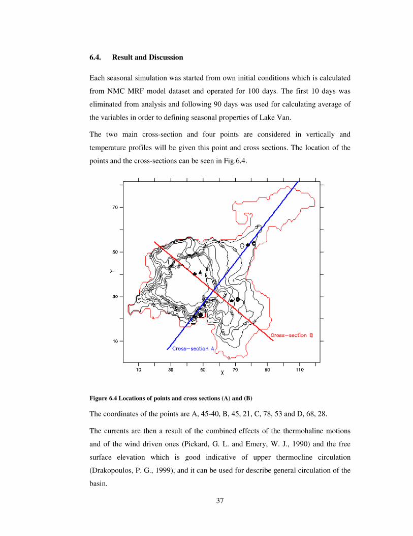
37
6.4. Result and Discussion
Each seasonal simulation was started from own initial conditions which is calculated
from NMC MRF model dataset and operated for 100 days. The first 10 days was
eliminated from analysis and following 90 days was used for calculating average of
the variables in order to defining seasonal properties of Lake Van.
The two main cross-section and four points are considered in vertically and
temperature profiles will be given this point and cross sections. The location of the
points and the cross-sections can be seen in Fig.6.4.
Figure 6.4 Locations of points and cross sections (A) and (B)
The coordinates of the points are A, 45-40, B, 45, 21, C, 78, 53 and D, 68, 28.
The currents are then a result of the combined effects of the thermohaline motions
and of the wind driven ones (Pickard, G. L. and Emery, W. J., 1990) and the free
surface elevation which is good indicative of upper thermocline circulation
(Drakopoulos, P. G., 1999), and it can be used for describe general circulation of the
basin.

38
The blue regions on the surface elevation figures are negative and red regions are
positive surface elevation. The negative value represents that cyclonic circulation
(anti-clock wise in the northern hemisphere and clockwise in the southern) and
positive means that anti-cyclonic circulation.
6.4.1. Fall
The wind is blowing from NNW and its velocity is about 1 m/s in fall. The seasonal
average of the air temperature is 19.2 °C and downward longwave heat flux is 303.26
W/m2, shortwave heat flux, 221.86 W/m2.
Figure 6.5 The time-averaged free surface elevation in cm (fall)
The free surface elevation for fall condition is shown in Fig.6.5. There is two main
circulation region can be seen. One of them is in Deveboynu Basin and the other is
Tatvan Basin region. The maximum value of the surface elevation is in the center of
the cyclonic circulation and its value is about 1 cm.

39
The surface circulation pattern can be seen in Fig.6.6 during fall. It is clear that gyres
are on the deepest part of the basin and the highest temperature regions because
surface elevation depends on wind stress, depth and density. In seasonal simulations,
density is only function of temperature (no salinity variations) and wind stress
uniformly over the whole region.
Figure 6.6 The time-averaged surface currents (fall)
There is a flow from Erci! Gulf (north-east region of the Lake Van) to Deveboynu
Basin and the cyclonic circulations are observed as presented in Fig.6.6. The
maximum velocity of the current is about 19 cm/s and the average value of flow field
is 1.5 cm/s.
Figure 6.7 show that vertical structure of the currents in points A-D. It must be a
deep flow at 25m in point C and it is the opposite direction of the surface current. In
B point, u component of the current changes its direction in spite of the strong
bathymetry gradient.

40
Figure 6.7 The vertical distribution of the current (bold black lines, u component of the current and bold red lines, v component) in fall

41
Figure 6.8 The time-averaged surface temperature in fall.
Temperature distribution is horizontally uniform in about 20 °C but in the deepest
part of the lake is colder than shallow region (Fig 6.8) but horizontal temperature
value is quite higher than the initial value of the lake (12 °C) because of the net heat
gain (downward minus upward heat flux). Moreover, it is fairly near to the average
atmospheric temperature (~19 °C) in this season.
The overall temperature distribution is controlled by circulation. The much more
warmed up shallow regions loss their heat energy because of the circulations and it is
transported to much colder region.
Following figures represent temperature distribution in cross-section A. The bold line
in Fig.6.9 represents that initial temperature (12 °C) value of the lake. Locations of
the cross-section can be seen in Fig.6.4.

42
Figure 6.9.The time-averaged temperature distribution in cross section (A) (fall)
The detailed plot of the vertical temperature distribution show closest view of the
surface region (Fig.6.10).
Figure 6.10 Detailed temperature distributions in cross-section A (first 100m)
As the cross-section A, Figure 6.11 and 6.12 show temperature profile of the cross-
section B. Both of the cross-sections are similar and the dense cold water lies in less
denser warm water.
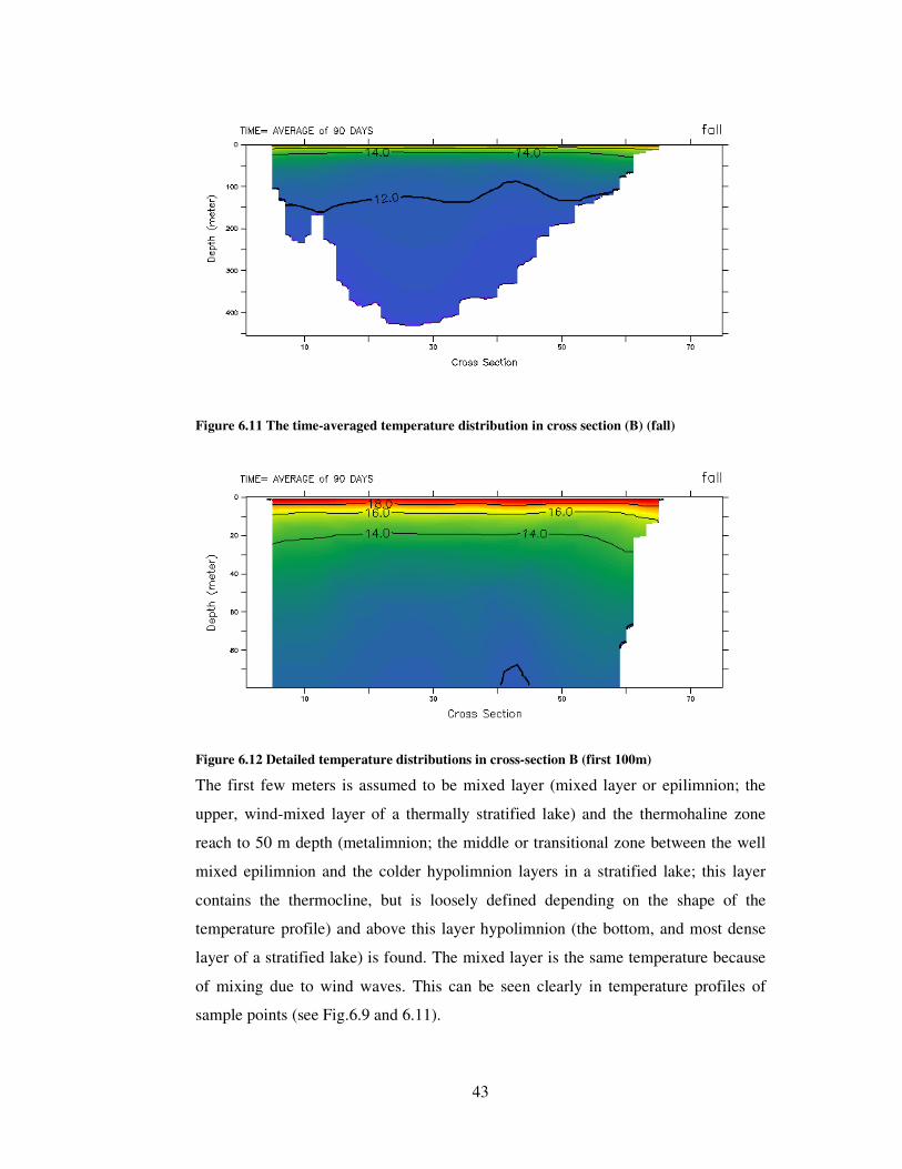
43
Figure 6.11 The time-averaged temperature distribution in cross section (B) (fall)
Figure 6.12 Detailed temperature distributions in cross-section B (first 100m)
The first few meters is assumed to be mixed layer (mixed layer or epilimnion; the
upper, wind-mixed layer of a thermally stratified lake) and the thermohaline zone
reach to 50 m depth (metalimnion; the middle or transitional zone between the well
mixed epilimnion and the colder hypolimnion layers in a stratified lake; this layer
contains the thermocline, but is loosely defined depending on the shape of the
temperature profile) and above this layer hypolimnion (the bottom, and most dense
layer of a stratified lake) is found. The mixed layer is the same temperature because
of mixing due to wind waves. This can be seen clearly in temperature profiles of
sample points (see Fig.6.9 and 6.11).
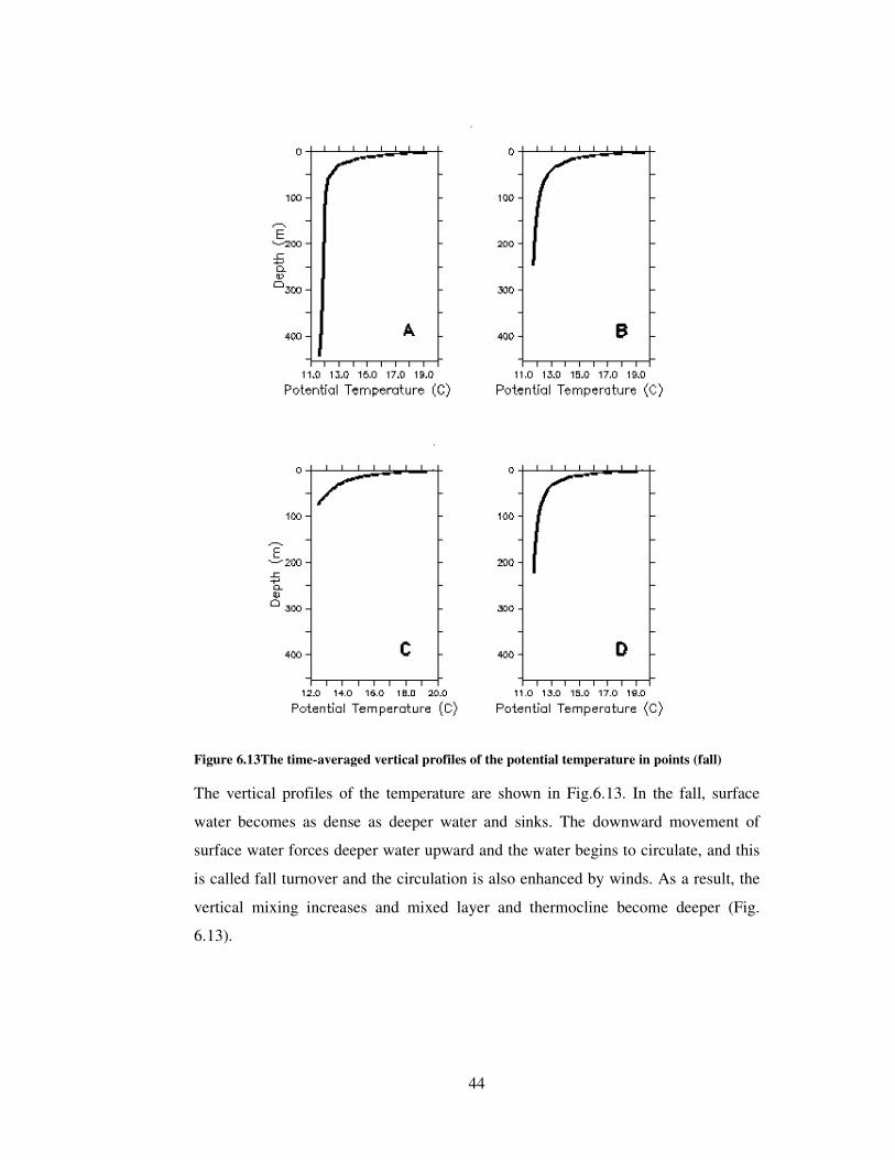
44
Figure 6.13The time-averaged vertical profiles of the potential temperature in points (fall)
The vertical profiles of the temperature are shown in Fig.6.13. In the fall, surface
water becomes as dense as deeper water and sinks. The downward movement of
surface water forces deeper water upward and the water begins to circulate, and this
is called fall turnover and the circulation is also enhanced by winds. As a result, the
vertical mixing increases and mixed layer and thermocline become deeper (Fig.
6.13).
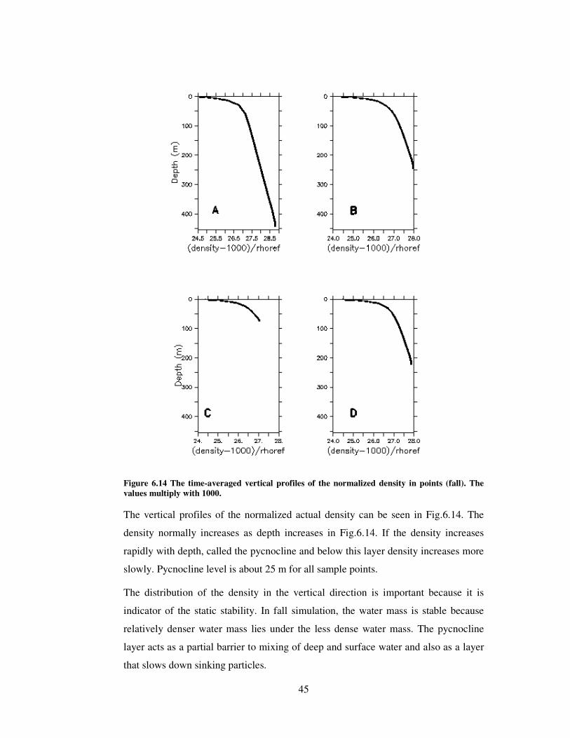
45
Figure 6.14 The time-averaged vertical profiles of the normalized density in points (fall). The values multiply with 1000.
The vertical profiles of the normalized actual density can be seen in Fig.6.14. The
density normally increases as depth increases in Fig.6.14. If the density increases
rapidly with depth, called the pycnocline and below this layer density increases more
slowly. Pycnocline level is about 25 m for all sample points.
The distribution of the density in the vertical direction is important because it is
indicator of the static stability. In fall simulation, the water mass is stable because
relatively denser water mass lies under the less dense water mass. The pycnocline
layer acts as a partial barrier to mixing of deep and surface water and also as a layer
that slows down sinking particles.

46
6.4.2. Winter
In the winter, the direction of the wind turns to the NNW from NE and the wind
speed is increases from 1 m/s to 3 m/s. The downward longwave radiation is
increases to 257.08 W/m2 as air temperature and downward shortwave radiation goes
down to 132.84 W/m2 because of the low sun angle. The seasonal average of the air
temperature is about 2 °C.
Figure 6.15 The time-averaged free surface elevation in cm (winter)
There is an anti-cyclonic circulation on the contrary of fall and it is located in Tatvan
Basin region. Strong winds causes to positive surface elevation which is the highest
rate in the middle of the gyre (see Fig.6.15). The maximum surface elevation is 2.3
cm and there is no thermal expansion effect over the surface elevation in winter.
The anti-cyclonic circulation can be seen more clearly in Fig.6.16 which shows the
surface current vectors.

47
The flow to the Erci! Gulf was observed in winter. Unlike fall, direction of the flow
is opposite way and much more strong because of the greater wind speed (from 1 m/s
in fall to 3 m/s in winter), the greater the frictional force acting on the lake surface
causes the stronger the surface current (see Fig.6.16) and there is a weak circulation
in Erek Fan region. The average flow speed is about 4 cm/s in the lake but it is the
maximum in the gyre region (~ 45 cm/s).
Figure 6.16 The time-averaged surface currents in winter.
Interesting features can be observed in Fig. 6.16 for winter. There is a surface current
which is opposite side of the wind direction, throughout the Erek Fan. It is transfer
the relatively warm water to the Ercis Gulf which is shallow and cold.
The vertical structure of the currents can be seen in Figure 6.17. The velocities are
higher than fall season because of the strong winds and it affects deeper part of the
lake. Unlike fall season, in C point direction of the u and v component of current
does not change and it is almost homogeny structure.

48
Figure 6.17 The vertical distribution of the current (bold black lines, u component of the current and bold red lines, v component) in winter
The depth of frictional influence (the depth at which the water velocity is opposite to
the surface velocity) is taken as a measure of the depth to which the surface wind
stress affects water motion and it is in the deeper than fall season (Fig.6.17).
For the real lake simulations, density only is a function of temperature because
salinity is constant and there is no water inflow with precipitation and outflow with
evaporation (VFLUX=0). The circulation can be divided into two parts, the
thermohaline and wind driven components. To obtain information about the reason
of the circulation this two components must be study. The gyre must be the
superposition of these two components.

49
The horizontal temperature distribution of the lake is different from fall case. In
winter, the net heat budget is negative value and lake is start to getting cold. The
coldest parts of the lake are shallow regions such as Erci" Gulf and Eastern Fan.
Figure 6.18 The time-averaged surface temperature in winter.
The average temperature of the lake surface is about 7.8 °C and the maximum value
is ~ 9 °C which is the center of the gyre (Fig.6.15 and 6.16). The coldest part of the
lake is Ercis Gulf region in which surface temperature is 3 °C (Fig.6.18).
The following figure show that the vertical cross-section of the temperature
distribution in Lake Van (Fig.6.19). The vertical distribution of the heat is almost
uniform.
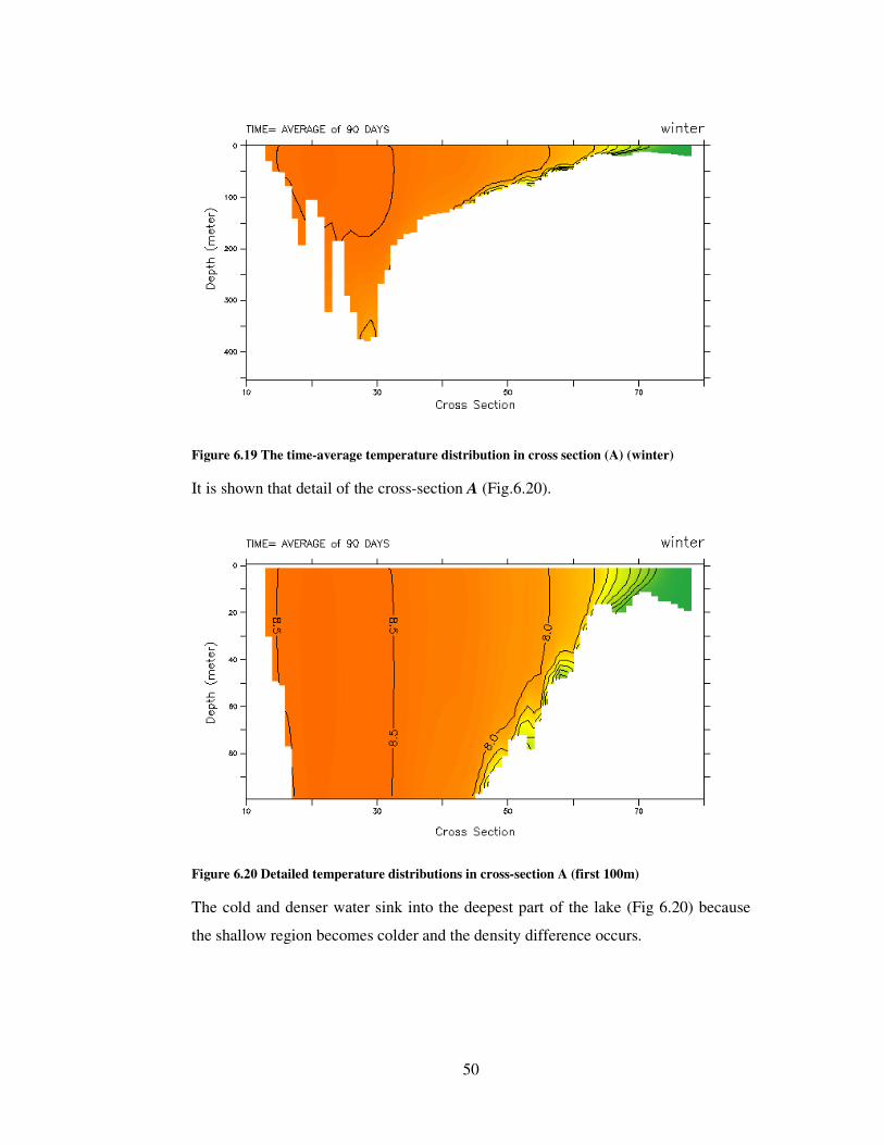
50
Figure 6.19 The time-average temperature distribution in cross section (A) (winter)
It is shown that detail of the cross-section A (Fig.6.20).
Figure 6.20 Detailed temperature distributions in cross-section A (first 100m)
The cold and denser water sink into the deepest part of the lake (Fig 6.20) because
the shallow region becomes colder and the density difference occurs.

51
Figure 6.21 The time-average temperature distribution in cross section (B) (winter)
The vertical profiles of the temperature are shown in Fig.6.22. Otherwise the fall
simulation, stratification does not appear in winter. The mixed layer can be seen
more clearly than fall season. All lake is mixed and temperature differences between
upper and lower levels are small.
In fact that surface temperature low and the mixed layer is deep in winter. It is
typically the warmest layer in the winter lies in hypolimnion.

52
Figure 6.22 The time-averaged vertical profiles of the potential temperature in points (winter)
In the winter, cooling of surface waters increases their density and they sink.
Continued cooling creates an isothermal water column. This water column is well
mixed and there is no seasonal thermocline (isothermal). This mixing continues until
surface freezes but there is no evidence to freezing in the Lake Van. This
phenomenon can be seen in Fig.6.22.

53
Figure 6.23 The time-averaged vertical profiles of the normalized density in points (winter). The values multiply with 1000.
There is a much smaller increase of density with depth than in fall and the seasonal
pycnocline is less evident (Fig 6.23). The density of lake is increasing rapidly until
bottom of the lake (no shear at the pycnocline).

54
6.4.3. Spring
The wind blowing from ENE direction and it is seasonal average is 3.2 m/s. The
downward longwave heat flux is 279.05 W/m2 and downward shortwave flux,
290.70 W/m2. The seasonal average of the air temperature is 10 °C.
Figure 6.24 The time-averaged free surface elevation in cm (spring)
Surface elevation show that the gyres which can be observed in winter, have not
appear in spring. The general flow field does not exist in this season (see Fig.6.24)
but there is a weak cyclonic circulation in Erek Fan-Deveboynu Basin region. The
maximum surface elevation is 0.12 cm.
Surface currents can be seen in Fig.6.25. The strong anti-cyclonic circulations in
winter weaken and disappear in spring. The maximum current speed is 4.5 cm/s and
the average value is 0.4 cm/s.
The highest wind speed is in spring and this must be cause more strong currents in
the lake but the current velocities is less than previous season.

55
Figure 6.25 The time-averaged surface currents in spring.
It fact that the winds and currents are intimately related but the reason of the
circulation is not only wind-driven, it also effected from horizontal temperature
distribution of the lake. In spring simulation, the lake is vertically uniform
(temperature and density distribution) and the temperature effect is not exist.
Fig.6.26 shows vertically profile of the u and v component of current. The velocities
of the current components are 10 times lower than the winter case in spite of strong
wind. In addition, it is behavior is chaotic.

56
Figure 6.26 The vertical distribution of the current (bold black lines, u component of the current and bold red lines, v component) in spring

57
Figure 6.27 The time-averaged surface temperature in spring.
In spring, temperature distribution over lake is uniform structure and the average
value is 12.3 °C (Fig 6.27). There is a little net heat gain but it is not sufficient to
create a big temperature differences in the lake. The vertical structure of the
temperature is same as horizontal, but the 12 °C isotherm is in the range from the
150-200 m.
After winter, the temperature and density of lake water becomes similar from top to
bottom. The uniform water density allows the lake to mix completely, recharging the
bottom water with oxygen and bringing nutrients up to the surface. This is called
spring overturn

58
Figure 6.28 The time-averaged vertical profiles of the potential temperature in (A-D) (spring)
The time-averaged vertical temperature distribution in sample points can be seen in
Fig.6.28. The vertical profile of potential temperature show that uniform distribution
form surface to bottom of the lake in spring.
The vertical temperature distribution is an indicator of the mixing process. In the
spring, stratification is weak and there is still mixing in the lake but at the end of the
spring the thermal stratification becomes strong and mixing stops.

59
Figure 6.29 The time-averaged vertical profiles of the normalized density in points (spring). The values multiply with 1000.
The density decreases rapidly as depth increases all the point (Fig 6.29). The water is
static stable in this season. There is no pycnocline layer. Temperature and density
distribution are harmonious in vertically.

60
6.4.4. Summer
In summer, wind is blowing from WNW, 1.2 m/s. The direction is same with spring
but it is much lighter. There is net heat gain in this season and downward longwave
heat flux is 357.10 W/m2 and shortwave heat flux is 368.96 W/m2. Average air
temperature is 29 °C during summer.
Figure 6.30 The time averaged surface elevation in summer.
The two gyres can be observed in the lake (Fig.6.30) and this two cyclonic
circulation region become stronger at the end of the summer (in fall season).
Deveboynu and Tatvan basin are the location of the gyres. The maximum surface
elevation in the center of gyre and its value is about 2 cm.
The gyres can be seen more clearly in Fig.6.31. The maximum current speed is 27
cm/s and the average value of it is 2 cm/s. There is a flow from Erci! Gulf to Tatvan
basin throughout Erek fan. The direction of the flow is same with fall season
simulation but in winter this direction is opposite (See Fig.6.31, 6.16 and 6.6).

61
Figure 6.31 the time averaged surface currents in summer.
The reason of the changing flow direction must be related with wind direction. In
winter, wind blowing from NE and the flow direction is to the Erci! Gulf but in
summer the wind is almost opposite direction and the direction of the current to the
Tatvan Basin.
In fall and spring, flow pattern is same as between winter and summer but the
velocity of the currents much smaller.
The following figure represent that the vertical structure of the current in chosen
sample points (Fig.6.32). The flow which is the throughout Erek Fan, can be seen in
Fig.6.32 C. The surface current changes its direction as depth increases.
The velocity of the current is larger than simulation of the spring season. It must be
increased wind speed and downward radiation because both of them apply forcing
(heat and momentum) into the lake and it is transform into mechanical energy in
order to conservation of the energy.

62
Figure 6.32 The vertical distribution of the current (bold black lines, u component of the current and bold red lines, v component) in summer

63
Figure 6.33 The time-averaged surface temperature in summer.
The lake surface temperature varies form 30 °C to 33 °C (Fig 6.33). The south-east
shore of the lake is warmer because of the wind introduced currents. The deep part of
the lake is a little colder than the shallow regions.
Following figures show the potential temperature profiles in cross-section A and B
(Fig.6.34, 35, 36 and 37). The stratification can be seen more clearly form figures.
The isotherm of initial temperature of the lake (12 °C) is in the 150m depth.
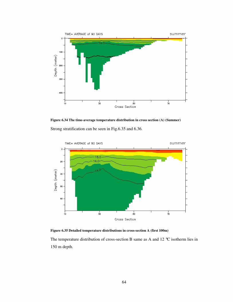
64
Figure 6.34 The time-average temperature distribution in cross section (A) (Summer)
Strong stratification can be seen in Fig.6.35 and 6.36.
Figure 6.35 Detailed temperature distributions in cross-section A (first 100m)
The temperature distribution of cross-section B same as A and 12 °C isotherm lies in
150 m depth.

65
Figure 6.36 Average temperature distribution for cross-section B (Summer)
Figure 6.37 Detailed temperature distributions in cross-section B (first 100m)

66
Figure 6.38 Vertical profiles of the potential temperature in A-D (Summer)
The lake becomes highly stratified and vertical mixing practically stops because of
the warm surface layer (less dense). The mixed layer is very shallow and
thermohaline layer is very thick.
The surface mixing layer is too thick and the thermohaline level is about 20 m depth
in all of the sample points (Fig 6.38). Above the thermohaline, temperature continues
to decreases slowly.
As a result, there is a thermal discontinuity between the epilimnion and hypolimnion
and in this layer temperatures rapidly changes.

67
Figure 6.39 The time-averaged vertical profiles of the normalized density in points (summer). The values multiply with 1000.
As the surface waters warm, they also become less dense than the water below. This
density difference soon becomes sufficient to prevent circulation within the water
column and the lake is divided into three regions (Fig 6.39).
The pycnocline level is in the same level with thermohaline and the density grows
with depth.

68
6.5. Comparison with the NOAA AVHRR data
In this section, SST data of the Lake Van which is estimated of monthly with NOAA
AVHRR image from February 1988 to January 1999 (Sari, M et al., 2000) are
compared with seasonal lake surface temperature data calculated with POM model.
Following table shows monthly minimum, maximum and average water surface
temperature of the Lake Van (Table 6.1).
Table 6.1 NOAA AVHRR Data (Water Surface Temperature) from (Sari, M. et al., 2000)
NOAA AVHRR Data
Season Month Min Max Ave Error ±
Dec. 6,60 9,70 8,50 0,73
Jan. 3,60 7,70 6,13 0,98
WIN
TER
Feb. -1,00 2,90 2,46 0,38
March 3,10 7,30 4,24 0,83
April 6,80 13,50 9,51 0,96
SPR
ING
May 9,60 14,90 11,48 0,87
June 13,50 17,70 15,46 0,98
July 19,10 22,40 20,64 1,13
SUM
MER
Aug. 18,40 22,40 21,34 0,54
Sept. 19,30 22,40 20,86 0,71
Oct. 12,00 16,10 14,82 0,86
AU
TUM
N
Nov. 7,90 12,20 10,87 1,25
Winter 3,07 6,77 5,70 0,70
Spring 6,50 11,90 8,41 0,89
Summer 17,00 20,83 19,15 0,88
AV
ERA
GE
Autumn 13,07 16,90 15,52 0,94
The seasonal averages of the AVHRR data are used for estimating differences with
POM model results. The next table shows the seasonal average POM data and the
difference (Table 6.2).
Table 6.2 Comparison of the AVHRR and POM Lake Surface Temperature (unit °C)
NOAA AVHRR Data POM Model Data Differences (AVHRR-POM)
Min Max Ave Min Max Ave Min Max Ave
Winter 3,07 6,77 5,70 2,93 8,74 7,80 0,14 -1,97 -2,11
Spring 6,50 11,90 8,41 12,16 12,37 12,22 -5,66 -0,47 -3,81
Summer 17,00 20,83 19,15 29,64 33,37 31,54 -12,64 -12,54 -12,39
Autumn 13,07 16,90 15,52 18,83 20,80 19,79 -5,76 -3,90 -4,27
The lake surface temperatures are higher than the AVHRR data for all of the
seasonal simulation results. This could be given initial temperature of Lake Van at
the beginning of the seasonal simulations (12 °C).

69
If the previous season average of lake surface temperature used in the seasonal
simulations of POM, the results would be much closer to AVHRR data but during
seasonal simulations the AVHRR data are unavailable and an average value was
used in simulations.
The highest differences are in the summer season and it is reach to 12 °C and the
minimum ones are in winter simulation case. This must be seasonal thermal
stratification of the lake. In summer, the lake is stratified and there is no mixing. As a
result, the thermal energy is forced to be thin layer of the lake (only 10-20 m).
However, there is no stratification in winter and the vertical mixing exists in the lake
and the thermal energy becomes diffused to whole lake volume.
The current, depth and rivers have an effect over the surface temperature distribution
in the Lake Van (Sari, M et al., 2000). This result is appropriate with seasonal model
simulations (see seasonal result of the POM).
Unfortunately, the complete absence of appropriate measurements does not allow a
more accurate evaluation of these simulations.
6.6. Future works
First of all the pressure gradient and hydrostatic inconsistency problem will be
solved using techniques which is explained in Chapter 4. The subtracting reference
density is used partially in POM but other techniques are tried for reduced error. It is
studied for implementation of new high order scheme by designer of model.
To simulating seasonal behavior of the Lake Van much accurate the NOAA AVHRR
data will be used as an initial condition.
The effects of rivers can be included into model because the fresh water flux and heat
transfer with river are affected hydrodynamic structure of the Lake Van.
The atmospheric model can be used for creating initial and time dependent boundary
condition of the POM. Coupled Atmosphere-Ocean model can be studied.
Inverse Ocean modeling techniques can be used for defining seasonal structure of the
Lake Van and NOAA AVHRR data can be used for this aim.

70
REFERENCES
Ahsan, A. K. M. Q. and Blumberg, A. F., 1999.Three-dimensional hydrothermal model of Onondaga Lake. Journal of Hydraulic Engineering, 125, 912-923.
Beletsky, D., O’Connor, W. P., Schwab, D. J., and Dietrich, D. E., 1997. Numerical Simulation of Internal Kelvin Waves and Coastal Upwelling Fronts. Journal of Physical Oceanography, 27, 1197-1215.
Blumberg, A. F. and Mellor, G. L., 1978.A coastal ocean numerical model. Mathematical Modeling of Estuarine Physics Proc. Int. Symp., 203-214.
Blumenthal, M. M., Kaaden, V. D., and Voldavetz, V. I., 1964.Catalogue of the active volcanoes of the world including sofatara fields. Part XVII Turkey and Caucasus. International Association of Volcanology, 23.
Bonnet, M. P., Poulin, M., and Devaux, J., 2000. Numerical modeling of thermal stratification in a lake reservoir. Methodology and case study. Aquatic Sciences, 62, 105-124.
Botte, V. and Kay, A., 2002. A Model of the wind-driven circulation in Lake Baikal. Dynamics of atmospheres and oceans, 35, 131-152
Chen, C., Ji, R., Schwab, D. J., Beletsky, D., Fahnenstiel, G. L., Jiang, M., Johengen, T. H., Vanderploeg, H., Eadie, B., Budd, J. W., Bundy, M. H., Gardner, W., Cotner, J., and Lavrentyev, P. J., 2002. A Model study of the coupled biological and physical dynamics in Lake Michigan. Ecological Modeling, 152, 145-168.
Chubarenko, B. V., Wang, Y., Chubarenko, I. P., and Hutter, K., 2001. Wind-driven current simulations around the Island Mainau (Lake Constance). Ecological Modeling, 138, 55-73.
Danaba%oglu, G. and McWilliams, J. C., 2000. An Upper Ocean Model for Short-Term Climate Variability. Journal of Climate, 13, 3380-3411.

71
Degens, E. T. and Kurtman, F., 1978. The Geology of Lake Van. Vol. 169, The Geology of Lake Van, The Mineral Research and Exploration Institute of Turkey, 158 pp.
Haney, R. L., 1991. On the Pressure Gradient Force over Steep Topography in Sigma Coordinate Ocean Models. Journal of Physical Oceanography, 21, 610-619
Hartmann, D. L., 1994. Global Physical Climatology. Vol. 56, International Geophysical Series, Academic Press, 411 pp.
Heinrich, J., Paul, J., and Lick, W., 1981. Temperatures and Currents in a stratified lake: A two dimensional analysis. Journal of Great Lakes Research, 7, 264-275.
Hodges, B. R., Imberger, J., Laval, B., and Appt, J., 2000. Modelling the Hydrodynamics of Stratified Lakes. HydroInformatics 2000 Conference, 1-14.
Hutter, K., 1984. Hydrodynamics of lakes. Springer-Verlag, viii, 341 pp.
Pickard, G. L., and Emery, W. J., 1990. Descriptive Physical Oceanography, An Introduction, 5th edition.. Butterworth Heinemann, 320 pp.
Kadıo!lu, M., $en, Z., and Batur, E. R., 1997. The greatest soda-water lake in the world and how it is influenced by climatic change. Annales Geophysicae, 15, 1489-1497.
Kelley, J. G. W., Hobgood, J. S., Bedford, K. W., and Schwab D. J., 1998. Generation of Three-Dimensional Lake Model Forecasts for Lake Erie. Weather and Forecasting, 13, 659-687.
Kempe, S., Khoo F., and Gürleyik Y., 1978. Hydrography of Lake Van and Its Drainage Area. Vol. 169, The Mineral Research and Exploration Institute of Turkey, 30-44 pp.
Mellor, G. L., 2003: User Guide to A Three-Dimensional, Primitive Equation, Numerical Model. June 1998 ed. 41 pp.
Mellor, G. L., 1991: An equation of state for numerical models of ocean and estuaries. Journal of Atmospheric and Oceanic Technology, 8, 609-611
Mellor, G. L., Oey L. Y., and Ezer, T., 1998. Sigma Coordinate Pressure Gradient Errors and the Seamount Problem. Journal of Atmospheric and Oceanic Technology, 15, 1122-1131

72
Mellor, G. L., Hakkinen S., Ezer T., and Patchen R., 2000. A generalization of a sigma coordinate ocean model and an intercomparison of model vertical grids, In: Ocean Forecasting: Theory and Practice, N. Pinardi (Ed.), Springer-Verlag, In Press, 2000.
Manshutkin, V. V., Astrakhantsev, G. P., Yegorava, N. B., Rukhovets, L. A., Simo, T. L., and Petrova, N. A., 1998. Mathematical modeling of the evolution and current conditions of the Ladoga Lake ecosystem. Ecological Modeling, 107, 1-24.
Sar!, M., Polat, I., Saydam, A. C., 2000. The Observation of Annual Variation of
Surface Temperature of The Lake Van by NOAA AVHRR Satellite
Images. Do'u Anadolu Bölgesi IV. Su Ürünleri Sempozyumu, 28-30
June 2000, Erzurum, Sempozyum Kitabı, 825-842 pp
Song, T. Y., 1998. A General Pressure Gradient Formulation for Ocean Models, Part I: Scheme design and Diagnostic Analysis. Monthly Weather Review, 126, 3213-3230
$en, Z., Kadıo!lu, M., and Batur, E. R., 2000. Stochastic Modelling of the Van Lake Monthly Level Fluctuations in Turkey. Theoretical and Applied Climatology, 65, 99-110.
Taguchi, K., Nakata, K., 1998. Analysis of water quality in Lake Hamana using a coupled physical and biochemical model. Journal of Marine Systems, 16, 107-132.
Tsvetova, E. A., 1999 Mathematical modeling of Lake Baikal hydrodynamics. Hydrobiologia, 407, 37-43
Wang, Y., and Hutter, K., 2002. Methods of substructuring in lake circulation dynamics. Advances in Water Resources, 23, 399-425
Wong, H. K., and Degens, E. T., 1978. The Bayhymetry of Lake Van, Eastern Turkey. Vol. 169, The Mineral Research and Exploration Institute of Turkey, 6-10 pp.

73
APPENDIX A
Appendix A.1 Free Surface Elevation after 50 days in ellipsoid, Latent + Sensible 20 W/m2
(a)
(c)
(b)
(d)
(f)

74
Appendix A.2 Free Surface Elevation after 50 days in ellipsoid, Latent + Sensible 40 W/m2
(a)
(c)
(b)
(d)
(e) (f)

75
Appendix A.3 Free Surface Elevation after 50 days in ellipsoid (EL), Latent + Sensible 80 W/m2
(a)
(c)
(b)
(d)
(e) (f)
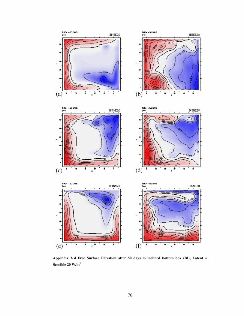
76
Appendix A.4 Free Surface Elevation after 50 days in inclined bottom box (BI), Latent +
Sensible 20 W/m2
(a)
(c)
(b)
(d)
(e) (f)

77
Appendix A.5 Free Surface Elevation after 50 days in inclined bottom box (BI), Latent +
Sensible 40 W/m2
(a)
(c)
(b)
(d)
(e) (f)

78
Appendix A.6 Free Surface Elevation after 50 days in inclined bottom box (BI), Latent +
Sensible 80 W/m2
(a)
(c)
(b)
(d)
(e) (f)

79
Appendix A.7 Free Surface Elevation after 50 days in flat bottom box (BI), Latent + Sensible 20
W/m2
(a)
(c)
(b)
(d)
(e) (f)

80
Appendix A.8 Free Surface Elevation after 50 days in flat bottom box (BC), Latent + Sensible 40
W/m2
(a)
(c)
(b)
(d)
(e) (f)

81
Appendix A.9 Free Surface Elevation after 50 days in flat bottom box (BC), Latent + Sensible 80
W/m2
(a)
(c)
(b)
(d)
(e) (f)

82
APPENDIX B
Appendix B.1 Potential temperature at 10 meter depth after 50 days in ellipsoid (EL), Latent +
Sensible 20 W/m2
(a)
(c)
(b)
(d)
(e) (f)

83
Appendix B.2 Potential temperature at 10 meter depth after 50 days in ellipsoid (EL), Latent +
Sensible 40 W/m2
(a)
(c)
(b)
(d)
(e) (f)

84
Appendix B.3 Potential temperature at 10 meter depth after 50 days in ellipsoid (EL), Latent +
Sensible 80 W/m2
(a)
(c)
(b)
(d)
(e) (f)

85
Appendix B.4 Potential temperature at 10 meter depth after 50 days in inclined bottom box (BI),
Latent + Sensible 20 W/m2
(a)
(c)
(b)
(d)
(e) (f)
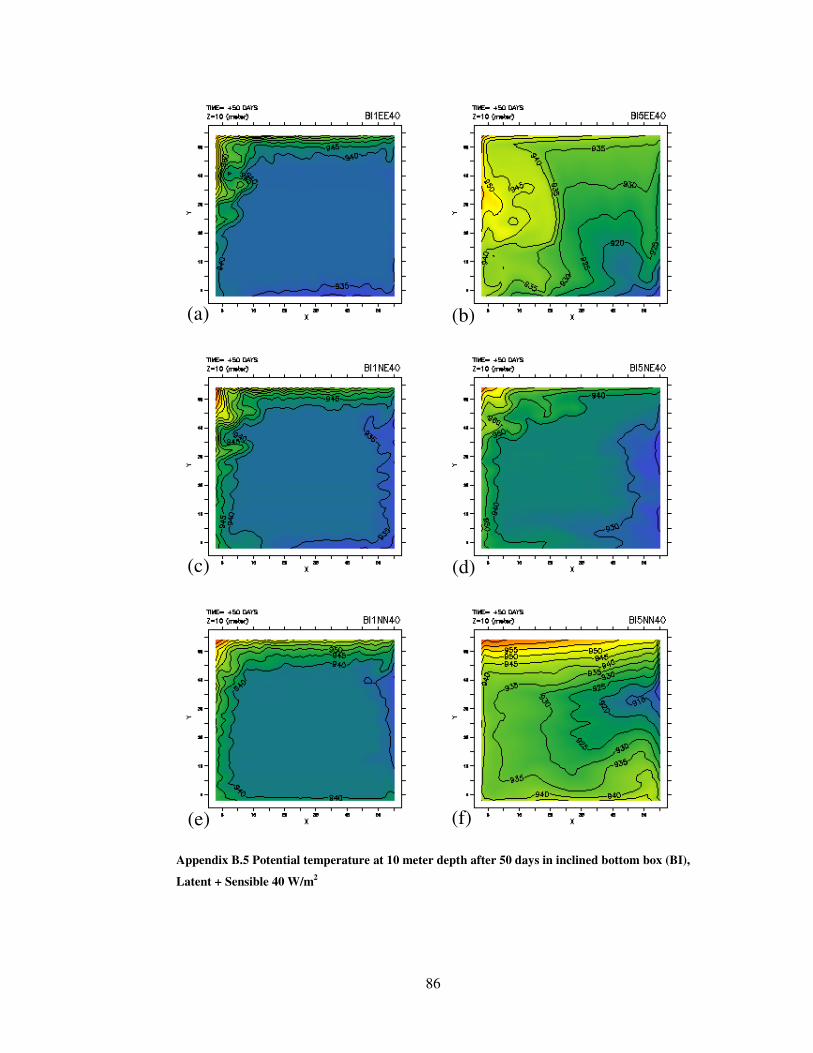
86
Appendix B.5 Potential temperature at 10 meter depth after 50 days in inclined bottom box (BI),
Latent + Sensible 40 W/m2
(a)
(c)
(b)
(d)
(e) (f)

87
Appendix B.6 Potential temperature at 10 meter depth after 50 days in inclined bottom box (BI),
Latent + Sensible 80 W/m2
(a)
(c)
(b)
(d)
(e) (f)

88
Appendix B.7 Potential temperature at 10 meter depth after 50 days in flat bottom box (BC),
Latent + Sensible 20 W/m2
(a)
(c)
(b)
(d)
(e) (f)

89
Appendix B.8 Potential temperature at 10 meter depth after 50 days in flat bottom box (BC),
Latent + Sensible 40 W/m2
(a)
(c)
(b)
(d)
(e) (f)

90
Appendix B.9 Potential temperature at 10 meter depth after 50 days in flat bottom box (BC),
Latent + Sensible 80 W/m2
(a)
(c)
(b)
(d)
(e) (f)

91
APPENDIX C
Appendix C.1 Surface currents (m/s) after 50 days in ellipsoid (EL), Latent + Sensible 20 W/m2
(a)
(c)
(b)
(d)
(f) (e)

92
Appendix C.2 Surface currents (m/s) after 50 days in ellipsoid (EL), Latent + Sensible 40 W/m2
(a)
(c)
(b)
(d)
(e) (f)

93
Appendix C.3 Surface currents (m/s) after 50 days in ellipsoid (EL), Latent + Sensible 80 W/m2
(a)
(c)
(b)
(d)
(e) (f)

94
Appendix C.4 Surface currents (m/s) after 50 days in inclined bottom box (BI), Latent +
Sensible 20 W/m2
(a)
(c)
(b)
(d)
(e) (f)

95
Appendix C.5 Surface currents (m/s) after 50 days in inclined bottom box (BI), Latent +
Sensible 40 W/m2
(a)
(c)
(b)
(d)
(e) (f)

96
Appendix C.6 Surface currents (m/s) after 50 days in inclined bottom box (BI), Latent +
Sensible 80 W/m2
(a)
(c)
(b)
(d)
(e) (f)
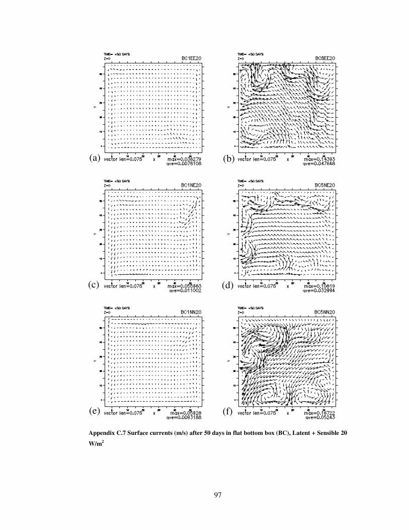
97
Appendix C.7 Surface currents (m/s) after 50 days in flat bottom box (BC), Latent + Sensible 20
W/m2
(a)
(c)
(b)
(d)
(e) (f)

98
Appendix C.8 Surface currents (m/s) after 50 days in flat bottom box (BC), Latent + Sensible 40
W/m2
(a) (b)
(e) (f)
(c) (d)

99
Appendix C.9 Surface currents (m/s) after 50 days in flat bottom box (BC), Latent + Sensible 80
W/m2
(c) (d)
(e) (f)
(a) (b)

100
BIOGRAPHY
Ufuk Utku Turunçoglu was born in 09 May 1977, Tokat. He studied his primary,
middle and high school in Istanbul and graduated from Istanbul Kurtulu! Lisesi in
1994.
He graduated from Meteorological Engineering, Istanbul Technical University in
2000. While he was working as a software developer, he continued his education
during two and half years and then he leaved his job and return back to the graduate
education.
He is still studying in Earth Sciences System Program of Department of Climate and
Ocean Sciences in Eurasia Institute of Earth Sciences, Istanbul Technical University.