ISTANBUL TECHNICAL UNIVERSITY ENERGY INSTITUTE

M.Sc. THESIS

JANUARY 2015

INVESTIGATION OF ISTANBUL’S NEOLITHIC AGE ANIMAL FINDINGS

BY NEUTRON ACTIVATION ANALYSIS

ISTANBUL TECHNICAL UNIVERSITY ENERGY INSTITUTE

Ayşe Tuba ÖNGÜL

Nuclear Researches Division

Radiation Science and Technology Programme

JANUARY 2015

ISTANBUL TECHNICAL UNIVERSITY ENERGY INSTITUTE



M.Sc. THESIS

Ayşe Tuba ÖNGÜL

(302111001)

Nuclear Researches Division

Radiation Science and Technology Programme

Thesis Advisor: Assist. Prof. Dr. Sevilay HACIYAKUPOĞLU

iii

Thesis Advisor : Assist. Prof. Dr. Sevilay HACIYAKUPOĞLU ..................

İstanbul Technical University

Jury Members : Prof. Dr. Sema AKYIL ERENTÜRK ..............................

İstanbul Technical University

Prof. Dr. Murat BELİVERMİŞ ..............................

Istanbul University

Ayşe Tuba Öngül, a M.Sc. student of ITU Institute of Energy student ID

302111001, successfully defended the thesis entitled “INVESTIGATION OF

ISTANBUL’S NEOLITHIC AGE ANIMAL FINDINGS BY NEUTRON

ACTIVATION ANALYSIS”, which she prepared after fulfilling the requirements

specified in the associated legislations, before the jury whose signatures are below.

Date of Submission : 17 December 2014

Date of Defense : 20 January 2015

v

I dedicate this thesis to my parents, Zuhal and Metin ÖNGÜL. I hope that this

achievement will complete the dream that you had for me all those many years ago

when you chose to give me the best education you could. And to my dear fiancee

Mustafa DURAN, for his unlimited patience and support.

vii

FOREWORD

I would like to express the deepest appreciation to my supervisor, Assist. Prof. Dr.

Sevilay HACIYAKUPOGLU from the Istanbul Technical University. I am

extremely grateful and indebted her. This thesis would not have been possible

without her expert, sincere and valuable guidance and encouragement extended to

me in every step of the time.

I would like to thank to Dr. Johannes STERBA from Technical University of Wien,

for acceptance of my request and his trust in me to spare his valuable time, insights

and directions, it has been a privilege to work with. And also to Michaela FOSTER,

I couldn’t have done without her great and devoted assistance in lab at Atominstitut.

In addition, a thank to Istanbul Archaeology Museum for their cooperation and

permission to include excavation findings and area maps as a part of my thesis. Also

to Rüveyda ILERI for her help in categorization and selection of the samples and to

biologist Sinem OZDEMIR, who by identifying the samples, helped immensely.

December 2014

Ayşe Tuba ÖNGÜL

ix

TABLE OF CONTENTS

Page

FOREWORD ............................................................................................................ vii TABLE OF CONTENTS .......................................................................................... ix ABBREVIATIONS ................................................................................................... xi LIST OF TABLES .................................................................................................. xiii LIST OF FIGURES ................................................................................................. xv SUMMARY ............................................................................................................ xvii ÖZET ........................................................................................................................ xix 1. INTRODUCTION .................................................................................................. 1 2. NEUTRON ACTIVATION ANALYSIS AND ARCHEOLOGY .................... 3

2.1 Fundamentals of Neutron Activation Analysis ................................................. 4 2.2 Nuclear Reactions .............................................................................................. 5 2.3 Activation With Neutrons .................................................................................. 6

2.3.1 Cross section ............................................................................................... 8 2.3.2 Decay rate ................................................................................................. 10 2.3.3 Induced activity ......................................................................................... 11

2.4 Derivation of the measurement equation.......................................................... 14 2.4.1 Standardization .......................................................................................... 17

2.4.1.1 Direct comparator method.................................................................. 17 2.4.1.2 Single comparator method ................................................................. 18 2.4.1.3 The k0-comparator method ................................................................. 19

2.4.2 NAA in Archaeology ................................................................................ 21 2.4.3 NAA in Marine Biota ................................................................................ 23

3. MATERIAL AND METHOD .......................................................................... 25 3.2 Site Information ............................................................................................. 25 3.3 Study Area ..................................................................................................... 27 3.4 Sample Properties .......................................................................................... 30 3.5 Preparation of Samples .................................................................................. 32 3.6 Irradiation and Counting ............................................................................... 34

4. RESULTS AND DISCUSSION ....................................................................... 43 4.1 Elemental analysis of Acanthocardia spinosa .............................................. 43 4.2 Elemental analysis of fish vertebra ............................................................... 44 4.3 Elemental analysis of Gastropods ................................................................. 44 4.4 Elemental analysis of Mytilus galloprovincialis ........................................... 45 4.5 Elemental analysis of Ostrea edulis .............................................................. 45 4.6 Elemental analysis of tortoise shell ............................................................... 46 4.7 Elemental analysis of non determined species .............................................. 46

5. CONCLUSION .................................................................................................. 51 REFERENCES ......................................................................................................... 55 CURRICULUM VITAE .......................................................................................... 59

xi

ABBREVIATIONS

A.D. : Anno Domini (After Christ)

BNL : Brookhaven National Laboratory

eV : Electron Volt

IAM : İstanbul Archaeology Museum

INAA : Instrumental Neutron Activation Analysis

keV : Kiloelectron Volt

LBL : Lawrence Berkeley Laboratory

N/D : Not defined

REE : Rare Earth Elements

SOM : Sea of Marmara

xiii

LIST OF TABLES

Page

Table 2.1 : Capture cross sections () and resonance integrals (I) (in barns) for

some typical activation targets .................................................................. 9

Table 3.1 : List of named samples according to soil depth. ...................................... 32

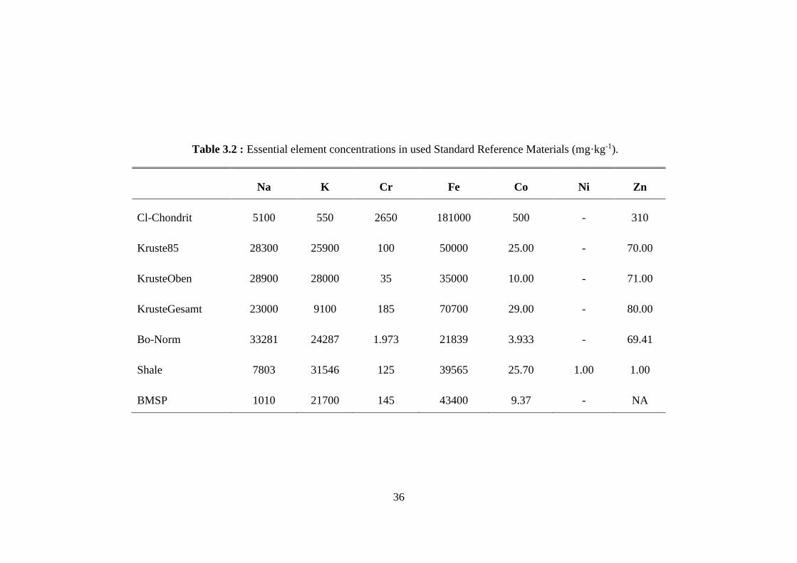
Table 3.2 : Essential element concentrations in used Standard Reference

Materials (mg·kg-1) ................................................................................. 36

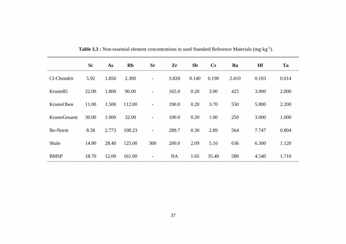
Table 3.3 : Non-essential element concentrations in used Standard Reference

Materials (mg·kg-1) ................................................................................. 37

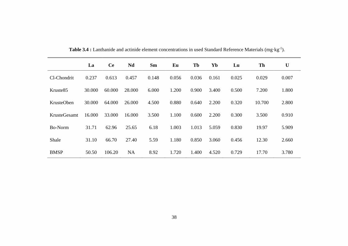
Table 3.4 : Lanthanide and actinide element concentrations in used Standard

Reference Materials (mg·kg-1) ................................................................ 38

Table 3.5 : Elements, activation products, half-lives, and γ-photon energies (sorted

by measurement sequences) ................................................................... 40

Table 4.1 : Element concentrations of Acanthocardia spinosa (mgkg-1) ................. 43

Table 4.2 : Element concentrations of fish vertebra (mgkg-1).................................. 44

Table 4.3 : Element concentrations of Gastropods (mgkg-1) ................................... 44

Table 4.4 : Element concentrations of Mytilus galloprovincialis (mgkg-1) ............. 45

Table 4.5 : Element concentrations of Ostrea edulis (mgkg-1) ................................ 46

Table 4.6 : Element concentrations of tortoise shell (mgkg-1) ................................. 46

Table 4.7 : Element concentrations of non determined species (mgkg-1) ................ 47

xv

LIST OF FIGURES

Page

Figure 2.1 : Distribution of neutrons according to their energies in nuclear reactor . 5 Figure 2.2 : Standardization curve for cobalt, irradiated in a thermal neutron flux of

1016 m-2 s-l for 10 d, showing the linear relationship between the mass

of the element and the induced activity. ................................................. 7 Figure 2.3 : Decay curve for 56Mn (t1/2 = 2.58 h), showing the semilogarithmic

relationship between length of decay and remaining activity. .............. 11 Figure 2.4 : Half-life values for typical activation products. .................................... 11 Figure 2.5 : Activation curve for 49Ca (t1/2) = 8.72 min)........................................... 12 Figure 2.6 : Activation curves for 64Cu (t1/2 = 12.70 h), showing the increase in

saturation activity with increasing neutron flux, from 1016 to 1018 n m-2

s-1 . ......................................................................................................... 13 Figure 3.1 : Marmaray Project Plan and Profile ....................................................... 26

Figure 3.2 : Archaeological Site at Yenikapı. ........................................................... 26 Figure 3.3 : Location of Theodosius. ........................................................................ 27 Figure 3.4 : The location of the excavation site in İstanbul. Digital image is

produced from Google Earth 4.3 .......................................................... 28 Figure 3.5 : Excavation Site Map (Courtesy of Istanbul Archaeological Museum). 29 Figure 3.6 : Location of collected findings. .............................................................. 30 Figure 3.7 : Samples from left to right respectively, 10C, 10F, 10L, 10R, 10E. ...... 30 Figure 3.8 : Samples from left to right respectively, 10K, 10P, 10I, 10Q, 10J......... 31 Figure 3.9 : Samples from left to right respectively, 10Q, 10N, 10A, 10D. ............. 31 Figure 3.10 : Samples from left to right respectively, 10H, 10M(1)(below),

10M(2)(above), 10B(1)(left), 10B(2)(right), 10G(right). ..................... 31 Figure 3.11 : Samples from left to right respectively, 10U(1)(tortoise shell),

10U(2)(fish vertebra), 10T(fish vertebra), 10S(fish vertebra). ............. 32 Figure 3.12 : Ultrasonic bath..................................................................................... 33 Figure 3.13 : Some of the samples after cleaning process, left to be dried............... 33 Figure 3.14 : Agate mortar. Plastic container and drilling ........................................ 33 Figure 3.15 : Sealing and engraving sample numbers to SuprasilTM quartz glass

vials, before irradiation. ........................................................................ 34 Figure 3.16 : TRIGA Mark II reactor of the Atominstitut ........................................ 35 Figure 3.17 : Gamma spectrometry system for NAA ............................................... 39 Figure 3.18 : Data acquisition flow sheet. ................................................................ 39 Figure 4.1 : Possible correlation between 10C, 10E and 10M(2). ............................ 47 Figure 4.2 : Essential element distribution in samples according to average

concentration values between species. .................................................. 48 Figure 4.3 : Lanthanides and actinides element distribution in samples according to

average concentration values between species. .................................... 48 Figure 4.4 : Non-essential element distribution in samples according to average

concentration values between species. .................................................. 49 Figure 4.5 : Element concentrations according to depth. .......................................... 49 Figure 5.1 : Fish species lanthanide and actinide series distribution. ....................... 51

xvi

Figure 5.2 : Zn concentrations for Mytilus g. and Ostrea e. species (mgkg-1). ........ 52

xvii



SUMMARY

In the study, the shells of Gastropods, Mytilus galloprovincialis, Acanthocardia

spinosa, Ostrea edulis, several fish vertebras as well as a tortoise shell were analyzed

by Neutron Activation Analysis. Results were compared to those from the literature

to contribute some subjects such as Istanbul’s oldest animals lived in Neolithic age

by evaluation of the results. Findings were collected from various depths on

Marmaray Site from Marmaray-Metro Project Archaeological Excavations at

Yenikapı, Istanbul. Neutron Activation Analysis technique was applied by irradiation

of samples at the TRIGA Mark II Research Reactor of the Atominstitut of Vienna

Technical University. In this frame concentrations of Na, K, Sc, Cr, Fe, Co, Ni, Zn,

As, Rb, Sr, Zr, Sb, Cs, Ba, La, Ce, Nd, Sm, Eu, Tb, Yb, Lu, Hf, Ta, W, Th and U

elements were determined.

The distribution of the elements in the shells was categorized into three groups. Of

these, first 7 elements (Na, K, Fe, Co, Cr, Ni, and Zn) were grouped together because

of their contribution to living organisms. Their average concentrations changes from

0,243 to 11,33 mgkg-1. Second ten elements (Sc, As, Rb, Sr, Zr, Sb, Cs, Ba, Hf, and

Ta) are not essential to living organisms, nevertheless may provide additional

information regarding e.g. pollution of the sea with further discussion. Their

concentrations are between 0,016 and 3,142 mgkg-1. The remaining ten elements

consists from Lanthanides and Actinides (La, Ce, Nd, Sm, Eu, Tb, Yb, Lu, Th and U)

which often called “Rare Earth Elements (REE’s)” are the most commonly

investigated elements with NAA. Their average concentration varies between 0,078

and 5,523 mgkg-1 throughout species. The main contribution of Zn and U comes

from fish bones and tortoise shell in accordance with the differences in chemical

composition between shells and bones of marine animals.

The characteristics of the 27 elements were studied separately in samples. It is

known that, in mollusk taxonomy, the elements have unique values. In other words,

element concentrations in various mollusk shells depend mainly on the taxonomic

characteristics of mollusks. In different bionomic environments, various element

distributions of the same species are attributed to the different geochemical

characters of the each environment. Considering that the organisms are the most

active and deterministic factors of the environment, data obtained in this study will

serve as a database for future research.

xix

ISTANBUL NEOLİTİK ÇAĞ CANLILARININ NÖTRON AKTİVASYON

ANALİZİ İLE INCELENMESİ

ÖZET

Nötron Aktivasyon Analizi, ister bilimsel ister teknik açıdan olsun, neredeyse akla

gelebilecek her alandaki örneklerde farklı miktarlardaki elementlerin (çok, az ve

eser), hem nicel hem de nitel analizlerinde uygulanılabilen hassas analitik bir

tekniktir. Örnek içinde bulunan kimyasal elementlerin nükleer aktivasyon yöntemi

ile radyoaktif hale getirilmesi prensibine dayanan bir kimyasal analiz yöntemidir. Bu

yöntemde elementler nötronlarla çarpıştırılarak radyoaktif hale getirildikten sonra,

uygun bir radyasyon algılama sistemi ile ölçülürler. Bombardımanda nötronlar

kullanıldığında yöntem nötron aktivasyon analizi (NAA) olarak adlandırılmaktadır.

Nötron bombardımanında, birim alandan birim zamanda geçen nötron sayısının çok

fazla olduğu reaktörler, bilinen en yaygın nötron kaynaklarıdır.

Analizi yapılacak malzemeye belirli bir süre düzgün ve kararlı bir nötron akısı

uygulandığında, nötronlar kinetik enerjisinin bir kısmını çekirdeğe ileterek saçılırlar

veya tüm enerjisini çekirdeğe ileterek çekirdek içinde yutulurlar. Bu durumdaki

çekirdekler fotonlar veya yüklü parçacıklar yayımlayarak kararlı hale geri dönerler.

Malzemenin içerdiği elementlerin kararlı izotoplardan nötron yutanlar, yeni ve

genellikle uyarılmış bir izotopa dönüşürler. Bu durumdaki çekirdekler 10-12 saniye

civarında çeşitli enerjilerde karakteristik gama fotonları salarak kararlı duruma

geçerler ki, bu gama ışınları ölçülmez, ya da kararlı izotop oluşabilir. Bu durumda da

gama radyasyonu ve ölçme söz konusu değildir, ya da oluşan izotop, algılanabilir bir

yarı ömürle bozumunu yaparak yeni bir elemente dönüşürken -ışını verir. Bu

ışınlar karakteristik enerji değerine sahip olup, o izotopun kimliğini belirler. Bu -

ışınlarının enerjileri saptanarak, onları doğuran elementlerin varlığı nitelik olarak ya

da şiddetleri ölçülerek, nicelikleri belirlenebilir.

Bu yöntemin uygulanmasında nüklitin tesir kesiti, nötron akısı, nötron kaynağı,

radyonüklit oluşumu ve bozunumu, sayım teknikleri, kimyasal ayırma gereksinimi,

sistematik hatalar ve örnekleme gibi konular detaylı olarak değerlendirilmelidir.

Nötron aktivasyon analizinin uygulanabilmesi için ilgilenilen elementin nükleer

reaksiyonlar gerçekleştiğinde yeterli miktarda radyoaktif izotop verebilmesi

gereklidir. Bu nedenle nükleer reaksiyonun gerçekleşme olasılığı (tesir kesiti), hedef

nüklitin izotopik bolluğu ve oluşan radyoizotopun yarı ömrünün yayımlanan

radyoaktivitenin ölçümüne yetecek kadar uzun olması gerekmektedir. Özellikle

matriste veya diğer safsızlıklarda meydana gelebilecek radyasyon nedeniyle

oluşabilecek girişimlerin anlaşılabilmesi ve giderilebilmesi için meydana gelen

radyasyonun tipi ve enerjisi de bilinmelidir.

Bu yöntemin bazı avantajları hassas, hızlı, ekonomik, kolay ve güvenilir bir yöntem

olmasıdır. Ayrıca genellikle, ışınlanan malzemede herhangi bir tahribat meydana

gelmez ve malzemede kimyasal değişim olmaz. Bir diğer özelliği de pek çok

elementin nötronlarla nükleer reaksiyona girmesinden dolayı aynı örnekte aynı anda

xx

birden fazla elementin nitel ve nicel analizi yapılabilir. Birçok element ve uygulama

için NAA, diğer metotlarla elde edilemeyecek, milyarda bir veya daha yüksek

hassaslık gösterir. Ek olarak, doğruluğu ve güvenilirliğinden dolayı NAA, yeni

prosedürler geliştirilirken veya diğer metotlar bir öncekiyle uyuşmayan sonuçlar

verdiğinde, genelde referans metot olarak da kullanılır. Başlangıçta yarı iletkenler

gibi yüksek saflıktaki malzemelerde, eser miktarda safsızlıkların tayininde kullanılan

NAA, günümüzde biyolojik bilimler (kan, doku, saç vb.), jeokimya, kriminoloji,

arkeoloji, çevre ile ilgili araştırmalar, endüstriyel uygulamalar gibi çeşitli alanlarda

kullanılmaktadır. Dünya çapında NAA araştırmaları o kadar yaygındır ki, her yıl

yaklaşık 100,000 örneğin analize alındığı tahmin edilmektedir.

2004 yılında Marmaray tüp geçit projesi inşaatı sırasında, İstanbul Arkeoloji

Müzeleri ve İstanbul Üniversitesi Sualtı Kültür Kalıntılarını Koruma Anabilim Dalı

tarafından başlatılan Yenikapı kazılarında, on binlerce eser ve Neolitik çağa ait

kalıntı gün yüzüne çıkmıştır. Geç Osmanlı döneminden başlayarak, erken Osmanlı,

Bizans, Roma, klasik ve arkeik dönem arkeoloji katmanlarının her evresinden

buluntularla birlikte İstanbul’un 8,500 yıllk süre içinde geçirdiği kültürel, sanatsal ve

jeolojik değişim, deniz ticareti, gemi teknolojisi, kent arkeolojisi, arkeo-botanik,

sanat tarihi, filoloji ve dendrokronoloji konularında önemli belgelere ulaşılmıştır.

Alanın sağladığı geniş tarih aralığı ve zengin geçmişi dolayısıyla çıkarılan örneklerde

analiz yapılarak önemli sonuçlara varılabilir.

Bu çalışmada, nükleer bir analiz yöntemi olan NAA yöntemi kullanılarak, deniz

canlısı örneklerindeki elementlerin belirlenmesi amaçlanmıştır. Bu kapsamda

kullanılan örnekler, İstanbul Arkeoloji Müzeleri Müdürlüğü’nün izniyle Yenikapı

Marmaray ve metro kazıları esnasında çıkarılan Neolitik Çağ Dönemine ait olduğu

belirlenmiş ve etütlük olarak tanımlanan deniz canlısı buluntularıdır.

Seçilen örnekler, kazı alanında çeşitli derinliklerden toplanmış olan, Gastropod

(Eklembacaklı), Mytilus galloprovincialis (Kara midye), Acanthocardia spinosa,

Ostrea edulis (İstiridye), balık omurgası ve kablumbağa kabuğundan oluşmaktadır.

Element miktarlarının belirlenmesi için Viyana Teknik Üniversitesi, ‘’Atominstitut’’

bünyesinde bulunan TRIGA Mark II nükleer araştırma reaktöründe, Nötron

Aktivasyon Analizi yöntemi kullanılmıştır. Bu amaçla buluntular önce çeşitli

işlemlerden geçirilerek dış kirliliklerden arındırılmıştır. Buluntular daha sonra

öğütülüp, belirlenen miktarlarda tartılıp, kuarz ışınlama tüplerine yerleştirilip,

kapatılıp reaktörde 30-40 saat sürelerde ışınlanmaya maruz bırakılmışlardır.

Işınlanan örneklerle birlikte çeşitli sertifikalı standart malzemeler de paketlenmiştir.

Uygulanan çeşitli soğuma ve ölçüm sürelerine göre Na, K, Sc, Cr, Fe, Co, Ni, Zn,

As, Rb, Sr, Zr, Sb, Cs, Ba, La, Ce, Nd, Sm, Eu, Tb, Yb, Lu, Hf, Ta, W, Th ve U

elementlerine dair veriler elde edilmiştir.

Örneklerdeki element dağılımı, canlı için hayati, hayati olmayan ve periyodik

tabloda lantanit ve aktinitler olarak sınıflandırılan eser elementler olmak üzere üç

grupta incelenmiştir. Birinci grupta incelenen 7 elementin (Na, K, Fe, Co, Cr, Ni ve

Zn) incelenen tüm türler için ortalama konsantrasyonu 0,243-11,33 mgkg-1; ikinci on

elementin (Sc, As, Rb, Sr, Zr, Sb, Cs, Ba, Hf ve Ta), 0,016-3,142 mgkg-1; geriye

kalan on elementin (La, Ce, Nd, Sm, Eu, Tb, Yb, Lu, Th, ve U) ise 0,078-5,523

mgkg-1 olarak bulunmuştur.

xxi

Çinko ve uranyum konsantrasyonları, balık omurgaları ve kablumbağa kabuğunun

kimyasal yapısıyla doğru orantılı olarak diğer örneklerden yüksek çıkmıştır. Aynı

zamanda kemiklerde eser elementlerin birikim davranışları gözlemlenebilmiştir.

Bu çalışma ile Neolitik Çağa ait deniz canlısı örneklerinde NAA ile element

konsantrasyonlarının belirlenmesinin, kendi aralarında ve modern literatur ile

karşılaştırılarak yorumlanmasının, Istanbul’un binlerce yıl önceki deniz canlılarının

özelliklerine ışık tutabileceği ve merak edilen sorulara cevap bulabileceği

düşünülmektedir.

1

1. INTRODUCTION

From the written sources, it has already been known that there was a port in

Yenikapı, Istanbul but never been searched before. In 2004, with the Marmaray Tube

Tunnel Project, began exploratory archaeological excavations, which have been

conducted jointly by the Istanbul Archaeological Museums and the Istanbul

University Department of Conservation of Underwater Cultural Heritages. For ten

years, findings from excavations uncovered the history of Istanbul from the late

Ottoman period back to the early Byzantine period, even to the Neolithic age. It

covers a period of 8,500 years of history of Istanbul. Also, relates to the cultural,

artistic and geological changes, maritime trade, ship technology, urban archaeology,

archaeobotanical, history of art, philology and so on [1].

In an area of 58 thousand square meters in Yenikapi, more than 35,000

archaeological findings have been unearthed to this date including the Harbor of

Theodosius, which was built by Theodosius I (379 - 395). It was the first trading port

in the city in the Early Byzantine Period and dates some 1,600 years back at a depth

between -1 and -6,30 meters [1].

It has been believed according to the findings that the Harbor was the center of the

world trade in the 4th century. Also, found, it had become mostly useless due to the

alluvium deposited by the stream, but it continued to be used until the 11th century

as a shelter by smaller ships and boats. The findings from the excavations shed light

on the history of the city of Istanbul. It provided data to track the changes undergone

by the Sea of Marmara for the last 10.000 years, with the help of the marine elements

layered between architectural remnants from the Neolithic Age [1].

Many disciplines prefer Neutron Activation Analysis (NAA) for the assessment of

elements present in samples. From archaeology, biomedicine, environmental

monitoring, food, forensic science, geological and inorganic materials, agriculture,

industrial applications, even to the quality assurance for determining the purity of

semiconductors.

2

So despite the developments of other analytical techniques, which use physical,

chemical and nuclear characteristics. It is still one of the primary method employed

in particular fields of science, depending on the purpose [2].

The greatest advantage of it is the fact that the samples do not have to be treated with

any chemical treatment, before or after the activation. It makes INAA non-

destructive and lower the probability of contamination from laboratory. It can

observe trace elements mostly at amounts in microgram to nanogram or even less.

Using the high selectivity of gamma-ray spectrometry allows the determination of

radionuclides simultaneously. It is usually used as a valuable reference for other

analysis methods. Worldwide application of NAA is so widespread; it is estimated

that approximately 100,000 samples undergo examination each year [3].

For provenance research, characterising archaeological materials with the application

of NAA has been used successfully and increasingly since Robert Oppenheimer

recognised it in the autumn of 1954. NAA’s results provide information to

archaeologists about questions such as sources of raw materials, trading practices, the

location of prehistoric production areas and the mobility patterns of ancient peoples.

Marine biogenic carbonates provide environmental records to the media in which

they have grown. Trace elements deposited in the marine system can be transferred

into the biota and may be affected by chemical and biological processes in the water

column, sediments and biota. Data obtained from the investigation can provide

indirect evidence of climatological diversity, or reveal unusual temporal changes in

elemental uptake possibly related to anthropogenic complexity of the environment

[4,5].

The aim of the study was to analyse the archaeological finds by NAA, compare the

results to those from the literature, and contribute some subjects such as Istanbul’s

oldest animals lived in Neolithic Age. By the evaluation of the results and also to

evaluate the levels of elemental concentrations, as well as bioaccumulation factors in

some of the species collected from the Yenikapı-Marmaray site. In this way,

questions may be addressed by the production, distribution and use of organic

substances in the ancient world. Most organic materials are subject to microbial, and

chemical degradation and thus useful biomarkers are only those that are sufficiently

robust to survive long-term deposition, such as shells and bone.

3

2. NEUTRON ACTIVATION ANALYSIS AND ARCHEOLOGY

NAA is very useful for trace and ultra-trace analysis of samples above all other

nuclear analytical techniques. When combined with spectroscopic methods it is an

efficient and precise method for multi-element investigation in trace element work.

Two years after Chadwick discovered the neutron in 1932, came the discovery of the

induced radioactivity by Irene Joliot and Frederic Curie. In the 1930s, one of the first

to use neutrons for producing artificial radioactive isotopes was Enrico Fermi.

Following the direction of his research George de Hevesy used it to study the rare

earth elements. When Hevesy and Levi found that the samples consists of certain

rare earth elements became radioactive after exposed to a source of neutrons, it

marked the beginning of neutron activation analysis. Thus in 1936, Hevesy and Levi,

released the first publication on the application of neutron activation analysis, which

stated, “… The usual chemical methods of analysis fail, as is well known, for most of

the rare earth elements and have to be replaced by spectroscopic, X-ray, and

magnetic methods. The latter methods can now be supplemented by the application

of neutrons to analytical problems by making use of the artificial radioactivity and

the high absorbing power of some of the rare earth elements for slow neutrons….”

[2].

Boyd was the one who suggested to term the procedure “… the method of radio

activation analysis …”, Alternatively, “… Activation analysis…”. In 1949 Boyd

proposed to name the process “… the method of radio activation analysis …”, Or,

more succinctly, “… activation analysis…” and he discussed the use of the “…

Chain-Reacting pile …” as a source of neutrons and an example of an analysis was

given.

With the advances in gamma-ray spectrometry and scintillation detectors, technique

was further improved as it provided much better radionuclide selectivity. Many

applications still needed chemical separations. But with the semiconductor detector’s

introduction in the beginning of 1960s, selectivity in gamma ray spectrometry was

4

increased to such an extent that radionuclides could be determined directly in a pool

of radioactivities and thus removing the need for chemical separations. It set the start

of INAA as an essential form of NAA and improved further by the multichannel

pulse height analysers and laboratory computers [2].

INAA has been found useful in many fields of science. The greatest advantage of it

is the fact that the samples do not have to be treated with any chemical treatment,

before or after the activation. It makes INAA non-destructive and lower the

probability of contamination from laboratory. In addition, interference from elements

like H, C, N, Si, can be eliminated because they do not produce radioactive products

during neutron activation thus ensuring the determination of other activities, clearer.

It can observe trace elements mostly at amounts in microgram to nanogram or even

less. Using the high selectivity of gamma-ray spectrometry allows the determination

of radionuclides simultaneously. The preparation of the samples is very easy. An

amount of it just needs to be weighed and place in a suitable container. The results

are not affected by the chemical or physical state of the elements.

Because of its accuracy and precision, it is still one of the primary methods employed

by the National Institute of Standards and Technology to certify the concentrations of

elements in standard reference materials. It is used for materials which required to be

pure to the highest degree, such as semi-conductors, archaeology, agriculture,

criminology, geochemistry, environmental monitoring, industrial applications,

health, human nutrition and even for art [6].

2.1 Fundamentals of Neutron Activation Analysis

Essentially, Neutron activation is the irradiation of a nucleus with neutrons to

produce radioactive species, usually referred to as the radionuclide. The number of

radionuclides produced, depend on the number of neutrons, the number of target

nuclei, and on the cross section, which defines the probability of activation

occurring. If the activation product is radioactive, it will decay with a characteristic

half-life. Consequently, the growth of activity during irradiation will depend on the

half-life of the product. The energy of the neutrons that are bombarding the nucleus

will dictate the type of interaction that occurs and consequently the nature of the

5

activation product. Therefore, if the nucleus is irradiated in a neutron flux of both

slow and fast neutrons, there may be more than one activation product.

Similarly, interferences may occur as the result of the same radionuclide being

produced by the activation of different target nuclei.

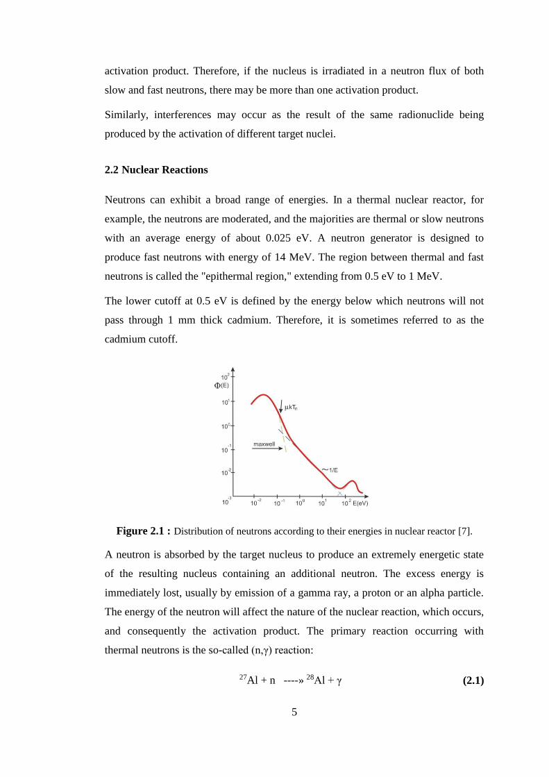
2.2 Nuclear Reactions

Neutrons can exhibit a broad range of energies. In a thermal nuclear reactor, for

example, the neutrons are moderated, and the majorities are thermal or slow neutrons

with an average energy of about 0.025 eV. A neutron generator is designed to

produce fast neutrons with energy of 14 MeV. The region between thermal and fast

neutrons is called the "epithermal region," extending from 0.5 eV to 1 MeV.

The lower cutoff at 0.5 eV is defined by the energy below which neutrons will not

pass through 1 mm thick cadmium. Therefore, it is sometimes referred to as the

cadmium cutoff.

Figure 2.1 : Distribution of neutrons according to their energies in nuclear reactor [7].

A neutron is absorbed by the target nucleus to produce an extremely energetic state

of the resulting nucleus containing an additional neutron. The excess energy is

immediately lost, usually by emission of a gamma ray, a proton or an alpha particle.

The energy of the neutron will affect the nature of the nuclear reaction, which occurs,

and consequently the activation product. The primary reaction occurring with

thermal neutrons is the so-called (n,γ) reaction:

27Al + n ----» 28Al + γ (2.1)

6

In this case, the highly energetic level of the product nucleus is de-excited by

emission of a gamma ray, which is called a prompt gamma, since it is emitted

immediately after activation. Fast neutrons induce different reactions. The absorption

occurs with either the ejection of a proton, in the case of an (n,p) reaction, for

example:

31P + n ----» 31Si + p (2.2)

or the production of an alpha particle, as in the case of an (n, α) reaction:

23Na + n ----» 20F + α (2.3)

The gamma rays, protons and alpha particles produced during these reactions are all

emitted spontaneously and therefore they are only detected if they are monitored

during the activation process. It is possible to see all three typical reactions: (n,γ),

(n,p) and (n,α), occurring with one target nucleus, for example in the case of 23Na

where not only the (n, α) reaction shown above occurs, but also the (n, y) and the

(n,p) reactions:

23Na + n ----» 24Na + γ (2.4)

23Na + n ----» 23Ne + p (2.5)

So in a neutron flux consisting of slow and fast neutrons the activation of 23Na will

result in the production of 24Na, 20F and 23Ne. These activation products are all

radioactive, but the product of a neutron-induced reaction may be a stable, naturally

occurring isotope of the particular element.

2.3 Activation With Neutrons

In a neutron-induced reaction, the growth of the product is dependent on the size of

the neutron flux. The larger the neutron flux, the greater the rates at which

interactions occur:

Activation rate neutron flux ()

The activation rate is also directly proportional to the number of target nuclei

present:

Activation rate number of nuclei present (N)

7

The number of target nuclei present will depend on the isotopic abundance of the

particular isotope of interest. For example, aluminum is composed entirely of stable

27Al, and so all the target nuclei will be the same.

However, there may be more than one isotope of an element, such as in the case of

calcium where there are six stable isotopes: 40Ca, 42Ca, 43Ca, 44Ca, 46Ca and 48Ca. As

an example, 48Ca is only present as 0.185 % of the total. In such cases the number of

target nuclei must be corrected for the isotopic abundance (a):

N=m a NA / M (2.6)

The number of target nuclei is, therefore, proportional to the mass of element

present. Since the growth of the activation product is proportional to the number of

target nuclei, it follows that the activation rate is commensurate with the mass of the

element:

Activation rate mass of element (m)

It is, therefore, possible to deduce the mass of element present from the induced

activity. It forms the basis of the neutron activation analysis technique. If the neutron

flux remains constant, then the "calibration curve" for an element can be determined

by plotting the induced activity against the mass of the element.

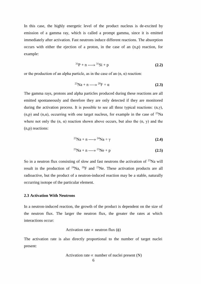
The simple relationship is shown in Figure 2.2 for 60Co using the data from the

compilation of calculated activities. The activity is given for a 10 d irradiation in a

thermal neutron flux of 1016 m-2 s-1. The slope is equivalent to the specific activity

and goes through zero.

Figure 2.2 : Standardization curve for cobalt, irradiated in a thermal neutron flux of 1016

m-2 s-l for 10 d, showing the linear relationship between the mass of the element and the

induced activity [8].

8

2.3.1 Cross section

The relationship between activation rate, the number of target nuclei and the neutron

flux is expressed by the term "cross section" (). The cross section is simply a

physical constant:

Activation rate = N (2.7)

N is the number of target nuclei, in atoms

is the neutron flux, in neutrons m-2 s-1

is the cross section, in m2

activation rate is in events s-1

Substituting:

N = m a NA / M (2.8)

into the expression for activation rate, it becomes:

Activation rate = m a NA / M (2.9)

Cross sections are usually expressed in barns which are 10-24 m2. As a rough guide, a

target nucleus with a cross section in the order of barns will activate well but a cross

section of millibarns indicates weak activation. It is important to remember that each

stable isotope of the same element will have a different cross section. Consequently,

one isotope may have a high cross section and become very active while another

isotope of the same element may have a small cross section and be activated to a

much smaller extent. It is, therefore, important to consider the cross sections when

deciding which target nuclide to use inactivation analysis.

The neutron cross section for a particular nucleus will depend on the energy of the

neutron. Many nuclei, particularly of small atomic number absorb thermal neutrons

with cross sections that decrease linearly with increasing velocity of the neutron

(known as 1/v absorbers). It is usual to refer to thermal cross sections for the

absorption of neutrons with an average velocity of 2,200 m s-1. Tables of cross

sections are available for activation with neutrons.

9

In the tables, the cross sections may be expressed in different forms. So, the total

cross section given for a particular target will be composed of a number of partial

cross sections, dependent on the activation process, including (n,γ), (n,p) and (n,α)

reactions. However for most thermal neutron activation the primary process is the

(n,γ) reaction involving the neutron radiative capture cross section ().

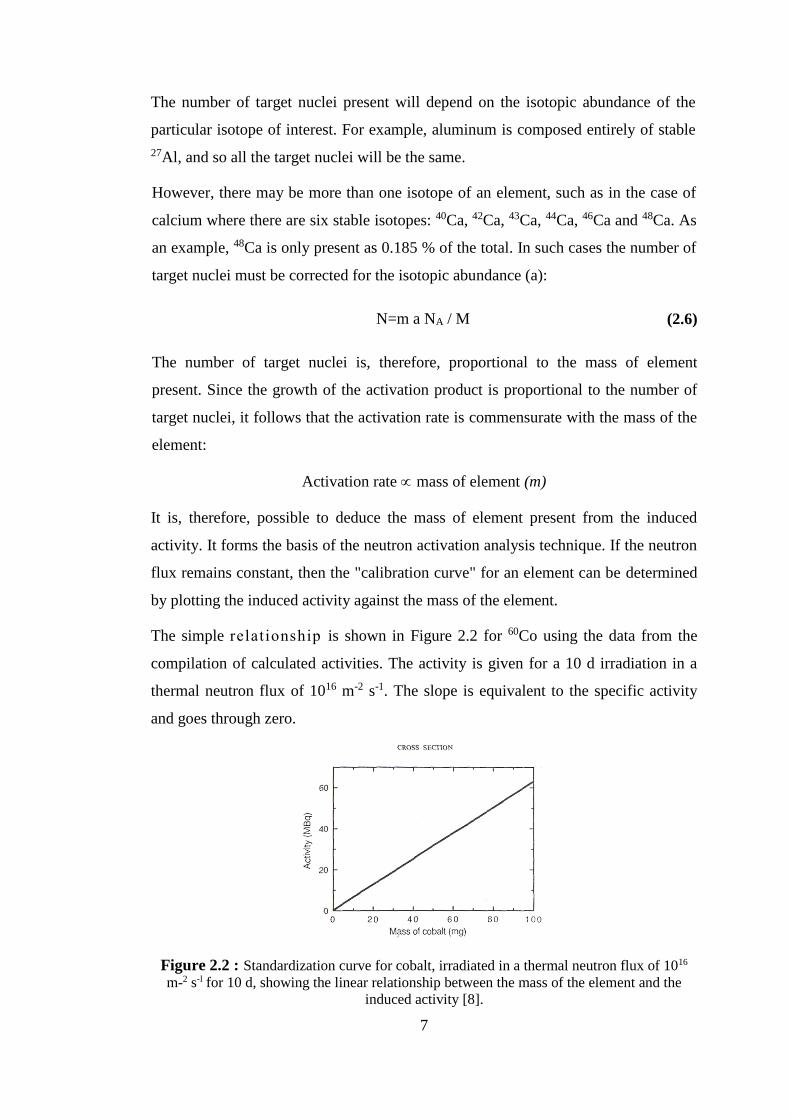
Not all target nuclei are 1/v absorbers, and there are many examples of nuclei that

preferentially absorb epithermal neutrons. At these higher energies, the neutron cross

section is referred to as the resonance integral and the radiative capture resonance

integral (I) is used. Some typical examples are shown in Table 1.1. It can be seen

from the cross section values that the lighter elements have thermal cross sections

and resonance integrals in the same order. They are the 1/v absorbers.

Table 2.1 : Capture cross sections () and resonance integrals (I) (in barns) for

some typical activation targets [8].

Target I Target I

23Na 0.4 0.31 63Cu 4.5 5.0

26Mg 0.038 0.026 75As 4.3 61 27Al 0.23 0.17 81Br 2.4 60

37CI 0.43 0.30 109Ag 91 1400

48Ca 1.09 0.89 139La 8.9 11.8

5IV 4.9 2.7 l52Sm 206 2970

50Cr 15.9 7.8 152Eu 9200 3300

55Mn 13.3 14.0 186W 37.9 485

58Fe 1.28 1.7 191Ir 954 3500

59Co 37.2 74 197Au 98.7 1550

On the other hand, the isotopes 109Ag, l52Sm and l97Au have vast resonance integrals

compared to the thermal cross sections, indicating that there are strong resonances in

the region above the cadmium cutoff energy. In these cases it is important to include

the resonance integral term in the calculation of the activation rate:

Activation rate = th N + I epi N (2.10)

th is the thermal neutron flux, epi is the epithermal neutron flux.

10

2.3.2 Decay rate

If the product nuclide in a neutron-induced reaction is stable the number of nuclei

produced is easily calculated from the activation equation by multiplying by the

length of irradiation, t:

Activation rate = N

Number of nuclei = N t

However, if the product nuclide is radioactive it will have a decay rate which must

be taken into account. The radionuclide produced will decay with a characteristic

half-life. If there are N* radioactive nuclei, the rate of decay of the nuclei is

proportional to N*:

Decay rate, dN*/dt* - N* (2.11)

= - N (2.12)

where is the decay constant, which has a characteristic value for each radionuclide.

If the equation is integrated between the limits N0* at time zero, and N* remaining at

time t:

N* = N0* exp(-t) (2.13)

It is from the above expression that the term half-life is derived since, for if the time

for half the nuclei to decay is defined as t1/2:

N0* / 2 = N()* exp (-t1/2) (2.14)

t1/2 = ln2/ = 0.693 / (2.15)

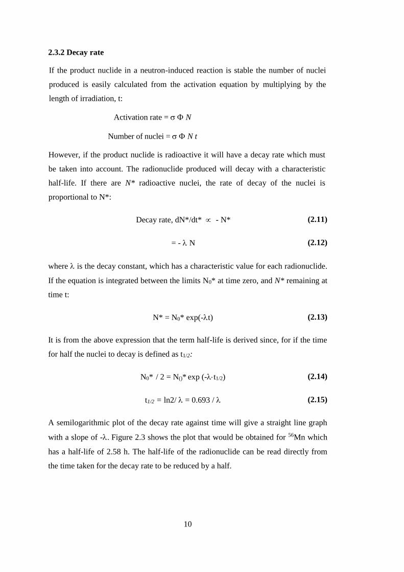
A semilogarithmic plot of the decay rate against time will give a straight line graph

with a slope of -. Figure 2.3 shows the plot that would be obtained for 56Mn which

has a half-life of 2.58 h. The half-life of the radionuclide can be read directly from

the time taken for the decay rate to be reduced by a half.

11

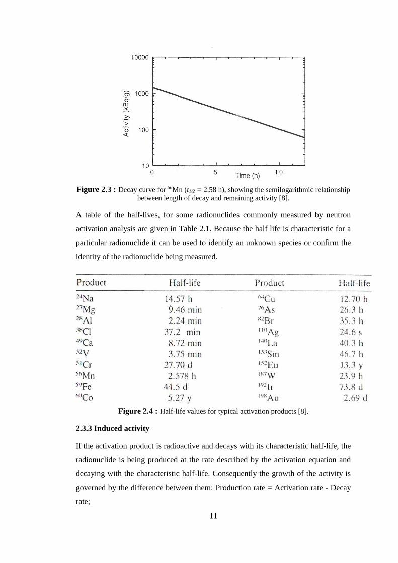
Figure 2.3 : Decay curve for 56Mn (t1/2 = 2.58 h), showing the semilogarithmic relationship

between length of decay and remaining activity [8].

A table of the half-lives, for some radionuclides commonly measured by neutron

activation analysis are given in Table 2.1. Because the half life is characteristic for a

particular radionuclide it can be used to identify an unknown species or confirm the

identity of the radionuclide being measured.

Figure 2.4 : Half-life values for typical activation products [8].

2.3.3 Induced activity

If the activation product is radioactive and decays with its characteristic half-life, the

radionuclide is being produced at the rate described by the activation equation and

decaying with the characteristic half-life. Consequently the growth of the activity is

governed by the difference between them: Production rate = Activation rate - Decay

rate;

12

dN* /dt = N - N* (2.16)

N* = N (1 – exp (-t)) / (2.17)

The activity or disintegration rate (A0), at the end of the irradiation time t, is then:

A0 = N* = N (1 – exp (-ti)) (2.18)

Consequently the growth of the induced activity with time is controlled by the half-

life of the activation product. This is demonstrated in Figure 2.4, where the growth

curve for 49Ca (t1/2 = 8.72 min) is plotted. It can be seen that the majority of the

activity is produced during the first two half-lives. When the irradiation time is very

long the expression for activity becomes close to the maximum possible activity for a

particular neutron flux, called the saturation activity (As):

As = N (2.19)

Figure 2.5 : Activation curve for 49Ca (t1/2) = 8.72 min) [8].

The saturation activity is independent of the half-life of the activation product and

depends only on the value of the neutron flux and neutron cross section. A plot of

activity induced in 64Cu for different neutron fluxes in Figure 2.5 shows the growth

of activity to saturation and how the saturation activity increases with neutron flux.

13

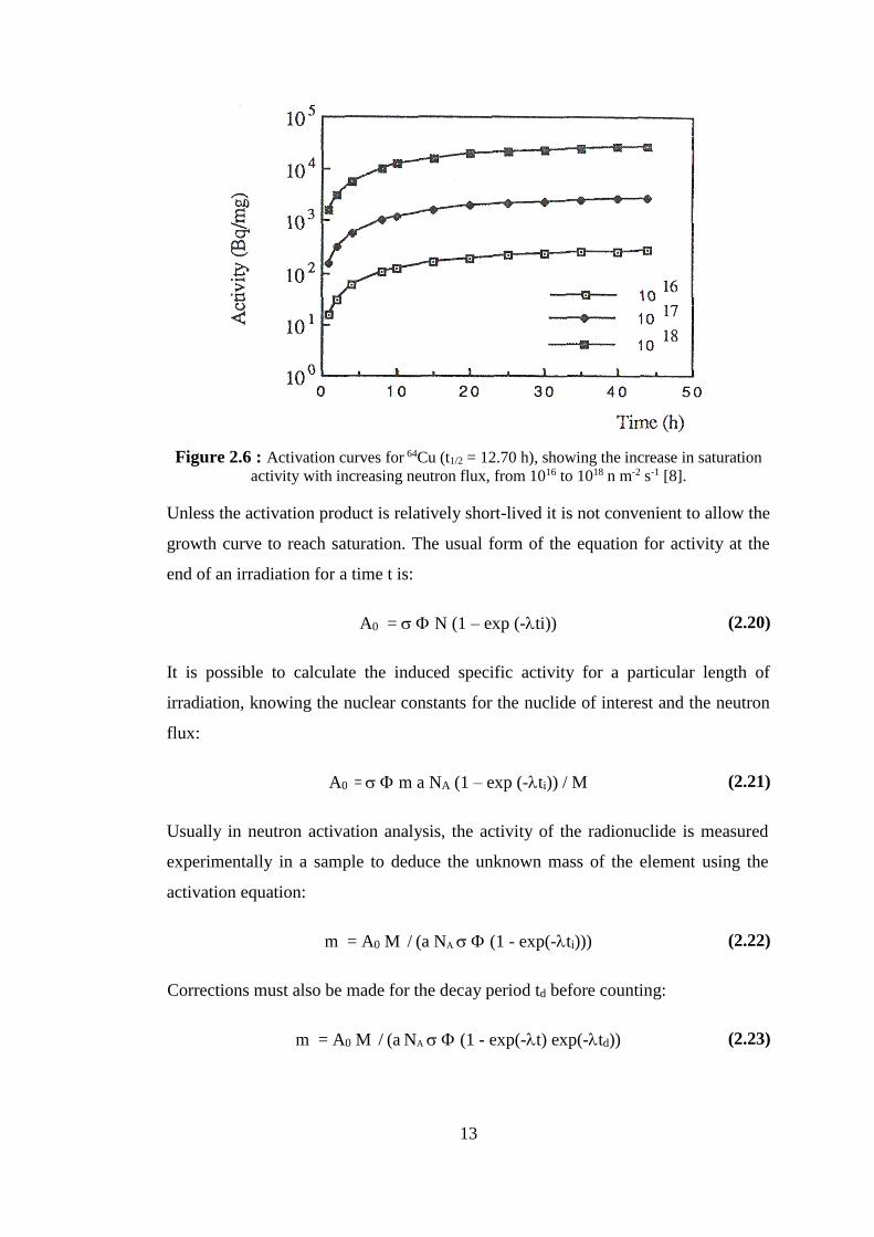
Figure 2.6 : Activation curves for 64Cu (t1/2 = 12.70 h), showing the increase in saturation

activity with increasing neutron flux, from 1016 to 1018 n m-2 s-1 [8].

Unless the activation product is relatively short-lived it is not convenient to allow the

growth curve to reach saturation. The usual form of the equation for activity at the

end of an irradiation for a time t is:

A0 = N (1 – exp (-ti)) (2.20)

It is possible to calculate the induced specific activity for a particular length of

irradiation, knowing the nuclear constants for the nuclide of interest and the neutron

flux:

A0 = m a NA (1 – exp (-ti)) / M (2.21)

Usually in neutron activation analysis, the activity of the radionuclide is measured

experimentally in a sample to deduce the unknown mass of the element using the

activation equation:

m = A0 M / (a NA (1 - exp(-ti))) (2.22)

Corrections must also be made for the decay period td before counting:

m = A0 M / (a NA (1 - exp(-t) exp(-td)) (2.23)

14

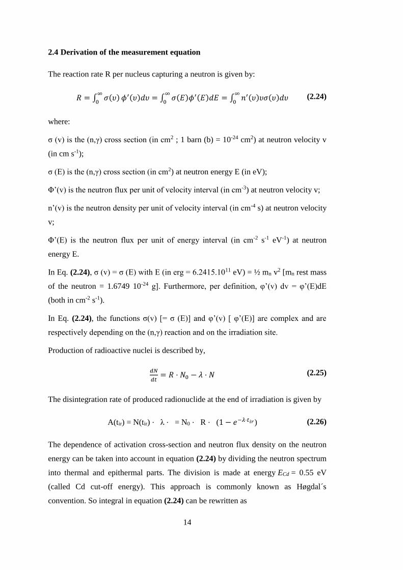
2.4 Derivation of the measurement equation

The reaction rate R per nucleus capturing a neutron is given by:

𝑅 = ∫ 𝜎(𝜐)∞

0𝜙′(𝜐)𝑑𝜐 = ∫ 𝜎(𝐸)𝜙′(𝐸)𝑑𝐸 = ∫ 𝑛′(𝜐)𝜐𝜎(𝜐)𝑑𝜐

∞

0

∞

0 (2.24)

where:

σ (v) is the (n,γ) cross section (in cm2 ; 1 barn (b) = 10-24 cm2) at neutron velocity v

(in cm s-1);

σ (E) is the (n,γ) cross section (in cm2) at neutron energy E (in eV);

Φ’(v) is the neutron flux per unit of velocity interval (in cm-3) at neutron velocity v;

n’(v) is the neutron density per unit of velocity interval (in cm-4 s) at neutron velocity

v;

Φ’(E) is the neutron flux per unit of energy interval (in cm-2 s-1 eV-1) at neutron

energy E.

In Eq. (2.24), σ (v) = σ (E) with E (in erg = 6.2415.1011 eV) = ½ mn v2 [mn rest mass

of the neutron = 1.6749 10-24 g]. Furthermore, per definition, φ’(v) dv = φ’(E)dE

(both in cm-2 s-1).

In Eq. (2.24), the functions σ(v) [= σ (E)] and φ’(v) [ φ’(E)] are complex and are

respectively depending on the (n,γ) reaction and on the irradiation site.

Production of radioactive nuclei is described by,

𝑑𝑁

𝑑𝑡= 𝑅 ⋅ 𝑁0 − 𝜆 ⋅ 𝑁 (2.25)

The disintegration rate of produced radionuclide at the end of irradiation is given by

A(tir) = N(tir) ⋅ λ ⋅ = N0 ⋅ R ⋅ (1 − 𝑒−𝜆⋅𝑡𝑖𝑟) (2.26)

The dependence of activation cross-section and neutron flux density on the neutron

energy can be taken into account in equation (2.24) by dividing the neutron spectrum

into thermal and epithermal parts. The division is made at energy ECd = 0.55 eV

(called Cd cut-off energy). This approach is commonly known as Høgdal´s

convention. So integral in equation (2.24) can be rewritten as

15

𝑅 = ∫ 𝑛(𝜐) ⋅ 𝜐 ⋅ 𝜎(𝜐)𝑑𝜐 + 𝑉𝐶𝑑

0∫ 𝑛(𝜐) ⋅ 𝜐 ⋅ 𝜎(𝜐)𝑑𝜐

0

𝑉𝐶𝑑 (2.27)

The first term can be integrated directly

∫ 𝑛(𝜐) ⋅ 𝜐 ⋅ 𝜎(𝜐)𝑑𝜐 = 𝜈0𝑉𝐶𝑑

0⋅ 𝜎0 ⋅ ∫ 𝑛(𝜐)𝑑𝜐 = 𝜈0 ⋅ 𝜎0 ⋅ 𝑛

∞

0 (2.28)

where,

𝑛 = ∫ 𝑛(𝜈)𝑑𝜈∞

0 (2.29)

is called the thermal neutron density, with Φth=nv0,

• Φth is the conventional thermal neutron fluence rate, m−2 s−1, for energies up to the

Cd cutoff energy of 0.55 eV;

• σ0 is the thermal neutron activation cross section, m2, at 0.025 eV;

• v0 is the most probable neutron velocity at 20 °C: 2200 m s−1.

The second term is re-formulated in terms of neutron energy rather than neutron

velocity and the infinite dilution resonance integral I0 – which effectively is also a

cross section (m2) – is introduced:

∫ 𝑛(𝜈)𝜈𝑑𝜈 = 𝜑𝑒𝑝𝑖 ∫𝜎(𝐸𝑛)𝑑𝐸𝑛

𝐸𝑛

𝐸𝑚𝑎𝑥

𝐸𝐶𝑑

∞

𝜈𝐶𝑑 (2.30)

with,

𝐼0 = ∫𝝈(𝑬𝒏)𝒅𝑬𝒏

𝑬𝒏

𝑬𝒎𝒂𝒙

𝑬𝑪𝒅 (2.31)

It is clear from this definition that the energy dependence of epithermal neutron flux

density is proportional to 1/E.

In the practice of nuclear reactors, the density of the epithermal neutron flux is not

following the inverse proportionality exactly. A small deviation can be measured and

therefore a parameter α is introduced as,

𝐼0(𝛼) = (1𝑒𝑉)𝛼 ∫𝜎(𝐸𝑛)𝑑𝐸𝑛

𝐸𝑛(1+𝛼)

𝐸𝑚𝑎𝑥

𝐸𝐶𝑑 (2.32)

The term for reaction rate can be rewritten as,

16

𝑅 = 𝜑𝑡ℎ𝜎0 + 𝜑𝑒𝑝𝑖𝐼0(𝛼) (2.33)

Expressing the ratio of the thermal neutron fluence rate and the epithermal neutron

fluence rate as f=Φth/Φepi and the ratio of the resonance integral and the thermal

activation cross section as Q0(α)= I0(α)/σ0, an effective cross section can be defined:

𝜎𝑒𝑓𝑓 = 𝜎0(1 +𝑄0(𝛼)

𝑓) (2.34)

t simplifies the Eq. (2.33) for the reaction rate to:

𝑅 = 𝜑𝑡ℎ𝜎𝑒𝑓𝑓 (2.35)

The nuclear transformations are established by measurement of the number of

nuclear decays. The number of activated nuclei N(ti,td) present at the start of the

measurement is given by:

N(ti,td,tm) = 𝑅𝑁0

𝜆(1 − 𝑒−𝜆𝑡𝑖)𝑒−𝜆𝑡𝑑 (2.36)

and the number of nuclei ΔN disintegrating during the measurement is given by:

ΔN(ti,td,tm) = 𝑅𝑁0

𝜆(1 − 𝑒−𝜆𝑡𝑖)𝑒−𝜆𝑡𝑑(1 − 𝑒−𝜆𝑡𝑚) (2.37)

in which td is the decay or waiting time, i.e. the time between the end of the

irradiation and the start of the measurement tm is the duration of the measurement.

Replacing the number of target nuclei N0 by (NAvm)/M and using the Eq. (2.35) for

the reaction rate, the resulting net counts C in a peak in the spectrum corresponding

with a given photon energy is approximated by the activation formula:

Np = ΔNγε = φthσeff 𝑁𝑎𝑣𝜃𝑚𝑥

𝑀𝑎(1 − 𝑒−𝜆𝑡𝑖)𝑒−𝜆𝑡𝑑(1 − 𝑒−𝜆𝑡𝑚)𝐼𝜀 (2.38)

with:

• Np is the net counts in the γ-ray peak of Eγ ;

• NAv is the Avogadro's number in mol−1;

• θ is isotopic abundance of the target isotope;

17

• mx is the mass of the irradiated element in g;

• Ma is the atomic mass in g mol−1;

• I is the gamma-ray abundance, i.e. the probability of the disintegrating nucleus

emitting a photon of Eγ (photons disintegration−1);

• ε is the full energy photopeak efficiency of the detector, i.e. the probability that an

emitted photon of given energy will be detected and contribute to the photopeak at

energy Eγ in the spectrum.

Although the photons emitted have energies ranging from tens of keVs to MeVs and

have high penetrating powers, they still can be absorbed or scattered in the sample

itself depending on the sample size, composition and photon energy. This effect is

called gamma-ray self attenuation.

Also, two or more photons may be detected simultaneously within the time

resolution of the detector; this effect is called summation. Eq. (2.38) can be simply

rewritten towards the measurement equation of NAA, which shows how the mass of

an element measured can be derived from the net peak area C:

mx = Np ∙𝑴𝒂

𝑵𝒂𝒗∙𝜽∙

𝝀

𝝋𝒕𝒉𝝈𝒆𝒇𝒇𝑰∙𝜺(𝟏−𝒆−𝝀𝒕𝒊)𝒆−𝝀𝒕𝒅(𝟏−𝒆−𝝀𝒕𝒎) (2.39)

2.4.1 Standardization

Standardization is based on the determination of the proportionality factors F that

relate the net peak areas in the gamma-ray spectrum to the amounts of the elements

present in the sample under given experimental conditions:

F=Np/M (2.40)

Both absolute and relative methods of calibration exist.

2.4.1.1 Direct comparator method

The unknown sample is irradiated together with a standard material (calibrator) that

contains a known amount of the element(s) of interest. Both are measured under the

same conditions (sample-to-detector distance, equivalent sample size and if possible

18

equivalent in composition). From the comparison of the net peak areas in the two

measured spectra the mass of the element of interest can be calculated:

𝑚𝑥(𝑢𝑛𝑘) = 𝑚𝑥(𝑐𝑎𝑙) ∙(

𝑵𝒑

𝒕𝒎𝒆−𝝀𝒕𝒅(𝟏−𝒆−𝝀𝒕𝒎))𝒖𝒏𝒌

(𝑵𝒑

𝒕𝒎𝒆−𝝀𝒕𝒅(𝟏−𝒆−𝝀𝒕𝒎))𝒄𝒂𝒍

(2.41)

in which mx(unk), mx(cal) mass of the element of interest, in the unknown sample

and the standard material, respectively in g.

In this procedure, when calculating the mass, neutron fluence rate, cross section, and

photopeak efficiency cancel out, and the remaining parameters are all known. This

calibration procedure is used when the highest degree of accuracy is desired.

For laboratories intended to get the full multi-element powers of INAA, the relative

calibration on the basis of element calibrators is not directly suitable. It takes

considerable effort to prepare multi-element calibrators for all 70 elements

measurable via NAA with an adequate degree of accuracy in a volume closely

matching the size and the shape of the samples.

2.4.1.2 Single comparator method

Multi-element INAA on basis of the relative calibration method is feasible when

performed according to the principles of the single comparator method. Assuming

stability in time of all relevant experimental conditions, calibrators for all elements

are co-irradiated each in turn with the chosen single comparator element. Once the

sensitivity for all elements relative to the comparator element has been determined

(expressed as the so-called k-factor, see below), only the comparator element has to

be used in routine measurements instead of individual calibrators for each element.

The single comparator method for multi-element INAA was based on the ratio of

proportionality factors of the element of interest and of the comparator element after

correction for saturation, decay, counting and sample weights defined the k-factor for

each element i as:

𝑘𝑖 =

(𝑀𝑎)𝑖,𝑐𝑎𝑙𝛾𝑐𝑜𝑚𝑝𝜃𝑐𝑜𝑚𝑝𝜎𝑒𝑓𝑓,𝑐𝑜𝑚𝑝

𝑀𝑖,𝑐𝑎𝑙𝛾𝑖,𝑐𝑎𝑙𝜀𝑖,𝑐𝑎𝑙𝜃𝑖,𝑐𝑎𝑙(𝜎𝑒𝑓𝑓)𝑖,𝑐𝑎𝑙 (2.42)

19

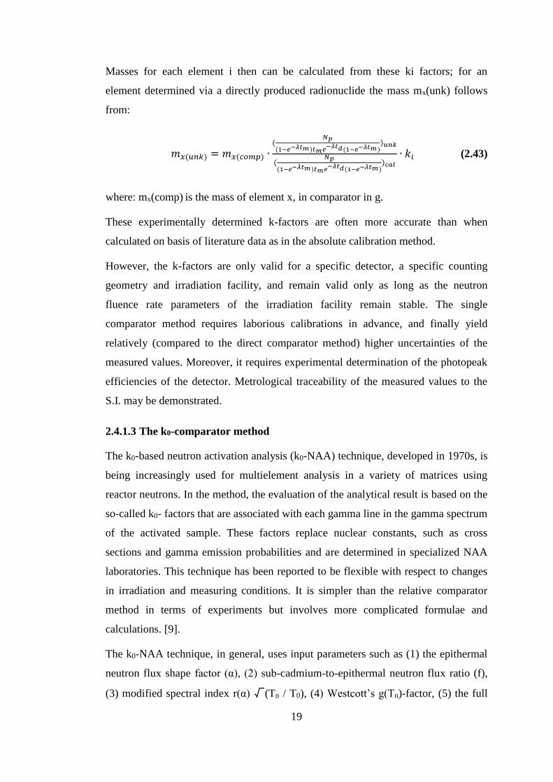
Masses for each element i then can be calculated from these ki factors; for an

element determined via a directly produced radionuclide the mass mx(unk) follows

from:

𝑚𝑥(𝑢𝑛𝑘) = 𝑚𝑥(𝑐𝑜𝑚𝑝) ∙(

𝑁𝑝

(1−𝑒−𝜆𝑡𝑚)𝑡𝑚𝑒−𝜆𝑡𝑑(1−𝑒−𝜆𝑡𝑚 ))𝑢𝑛𝑘

(𝑁𝑝

(1−𝑒−𝜆𝑡𝑚)𝑡𝑚𝑒−𝜆𝑡𝑑(1−𝑒−𝜆𝑡𝑚))𝑐𝑎𝑙

∙ 𝑘𝑖 (2.43)

where: mx(comp) is the mass of element x, in comparator in g.

These experimentally determined k-factors are often more accurate than when

calculated on basis of literature data as in the absolute calibration method.

However, the k-factors are only valid for a specific detector, a specific counting

geometry and irradiation facility, and remain valid only as long as the neutron

fluence rate parameters of the irradiation facility remain stable. The single

comparator method requires laborious calibrations in advance, and finally yield

relatively (compared to the direct comparator method) higher uncertainties of the

measured values. Moreover, it requires experimental determination of the photopeak

efficiencies of the detector. Metrological traceability of the measured values to the

S.I. may be demonstrated.

2.4.1.3 The k0-comparator method

The k0-based neutron activation analysis (k0-NAA) technique, developed in 1970s, is

being increasingly used for multielement analysis in a variety of matrices using

reactor neutrons. In the method, the evaluation of the analytical result is based on the

so-called k0- factors that are associated with each gamma line in the gamma spectrum

of the activated sample. These factors replace nuclear constants, such as cross

sections and gamma emission probabilities and are determined in specialized NAA

laboratories. This technique has been reported to be flexible with respect to changes

in irradiation and measuring conditions. It is simpler than the relative comparator

method in terms of experiments but involves more complicated formulae and

calculations. [9].

The k0-NAA technique, in general, uses input parameters such as (1) the epithermal

neutron flux shape factor (α), (2) sub-cadmium-to-epithermal neutron flux ratio (f),

(3) modified spectral index r(α) √(Tn / T0), (4) Westcott’s g(Tn)-factor, (5) the full

20

energy peak detection efficiency (εp), and (6) nuclear data on Q0 (ratio of resonance

integral (I0) to thermal neutron cross section (σ0) and k0. The parameters from (1) to

(4) are dependent on each irradiation facility and the parameter (5) is dependent on

each counting facility. The neutron field in a nuclear reactor contains an epithermal

component that contributes to the sample neutron activation. Furthermore, for

nuclides with the Westcott’s g(Tn)-factor different from unity, the Høgdahl

convention should not be applied and the neutron temperature should be introduced

for application of a more sophisticated formalism, the Westcott formalism.

These two formalisms should be taken into account in order to preserve the accuracy

of k0-method. The k0-NAA method is at present capable of tackling a large variety of

analytical problems when it comes to the multi-element determination in many

practical samples.

During the three last decades Frans de Corte and his co-workers focused their

investigations to develop a method based on co-irradiation of a sample and a neutron

flux monitor, such as gold and the use of a composite nuclear constant called k0-

factor. In addition, this method allows to analyze the sample without use the

reference standard like INAA method [9].

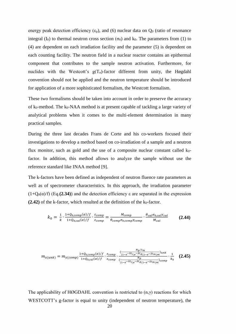
The k-factors have been defined as independent of neutron fluence rate parameters as

well as of spectrometer characteristics. In this approach, the irradiation parameter

(1+Q0(α)/f) (Eq.(2.34)) and the detection efficiency ε are separated in the expression

(2.42) of the k-factor, which resulted at the definition of the k0-factor.

𝑘0 = 1

𝑘∙

1+𝑄0,𝑐𝑜𝑚𝑝(𝛼) 𝑓⁄

1+𝑄0,𝑐𝑎𝑙(𝛼) 𝑓⁄∙

𝜀𝑐𝑜𝑚𝑝

𝜀𝑐𝑜𝑚𝑝=

𝑀𝑐𝑜𝑚𝑝

𝜃𝑐𝑜𝑚𝑝𝜎0,𝑐𝑜𝑚𝑝𝛾𝑐𝑜𝑚𝑝∙

𝜃𝑐𝑎𝑙𝜎0,𝑐𝑎𝑙𝛾𝑐𝑎𝑙

𝑀𝑐𝑎𝑙 (2.44)

𝑚𝑥(𝑢𝑛𝑘) = 𝑚𝑥(𝑐𝑜𝑚𝑝)1+𝑄0,𝑐𝑜𝑚𝑝(𝛼) 𝑓⁄

1+𝑄0,𝑐𝑎𝑙(𝛼) 𝑓⁄∙

𝜀𝑐𝑜𝑚𝑝

𝜀𝑐𝑜𝑚𝑝∙

(𝑁𝑝 𝑡𝑚⁄

(1−𝑒−𝜆𝑡𝑖)𝑒−𝜆𝑡𝑑(1−𝑒−𝜆𝑡𝑚)𝑚)𝑢𝑛𝑘

(𝑁𝑝

(1−𝑒−𝜆𝑡𝑖)𝑒−𝜆𝑡𝑑(1−𝑒−𝜆𝑡𝑚)𝑚)𝑐𝑜𝑚𝑝

∙1

𝑘0

(2.45)

The applicability of HØGDAHL convention is restricted to (n,γ) reactions for which

WESTCOTT’s g-factor is equal to unity (independent of neutron temperature), the

21

cases for which WESTCOTT’s g = 1, such as the reactions 151Eu(n, γ) and 176Lu(n, γ)

are excluded from being dealt with. Compared with relative method k0-NAA is

experimentally simpler (it eliminates the need for multi-element standards, but

requires more complicated calculations.

Summarizing, relative calibration by the direct comparator method renders the lowest

uncertainties of the measured values whereas metrological traceability of these

values to the S.I. can easily be demonstrated. As such, this approach is often

preferred from a metrological viewpoint.

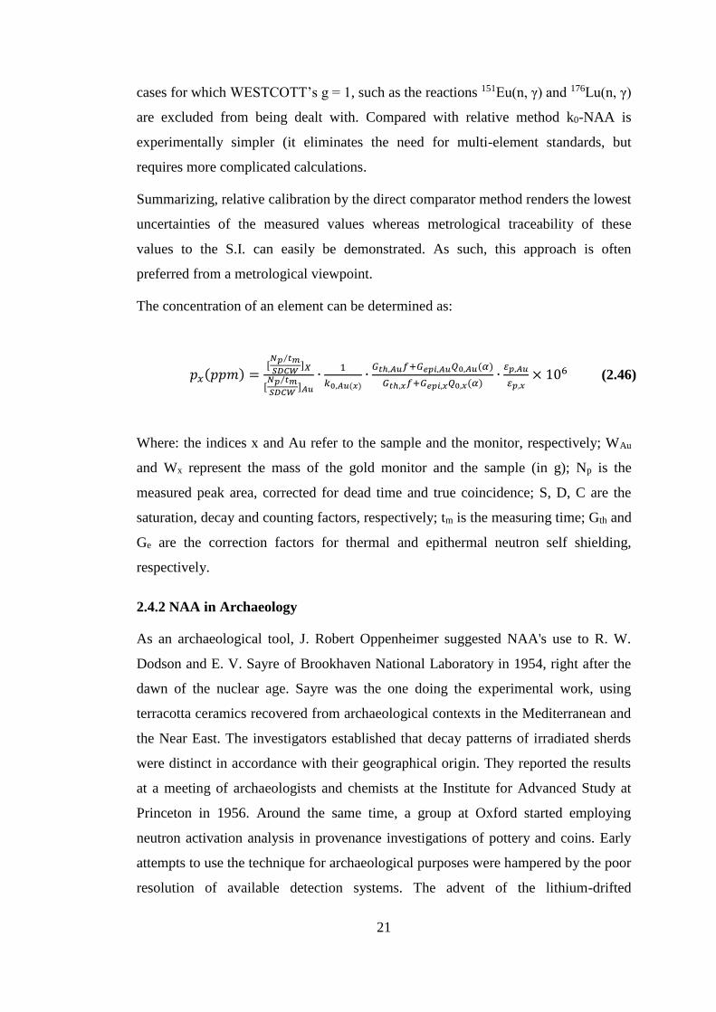
The concentration of an element can be determined as:

𝑝𝑥(𝑝𝑝𝑚) =[𝑁𝑝 𝑡𝑚⁄

𝑆𝐷𝐶𝑊]𝑋

[𝑁𝑝 𝑡𝑚⁄

𝑆𝐷𝐶𝑊]𝐴𝑢

∙1

𝑘0,𝐴𝑢(𝑥)∙

𝐺𝑡ℎ,𝐴𝑢𝑓+𝐺𝑒𝑝𝑖,𝐴𝑢𝑄0,𝐴𝑢(𝛼)

𝐺𝑡ℎ,𝑥𝑓+𝐺𝑒𝑝𝑖,𝑥𝑄0,𝑥(𝛼)∙

𝜀𝑝,𝐴𝑢

𝜀𝑝,𝑥× 106 (2.46)

Where: the indices x and Au refer to the sample and the monitor, respectively; WAu

and Wx represent the mass of the gold monitor and the sample (in g); Np is the

measured peak area, corrected for dead time and true coincidence; S, D, C are the

saturation, decay and counting factors, respectively; tm is the measuring time; Gth and

Ge are the correction factors for thermal and epithermal neutron self shielding,

respectively.

2.4.2 NAA in Archaeology

As an archaeological tool, J. Robert Oppenheimer suggested NAA's use to R. W.

Dodson and E. V. Sayre of Brookhaven National Laboratory in 1954, right after the

dawn of the nuclear age. Sayre was the one doing the experimental work, using

terracotta ceramics recovered from archaeological contexts in the Mediterranean and

the Near East. The investigators established that decay patterns of irradiated sherds

were distinct in accordance with their geographical origin. They reported the results

at a meeting of archaeologists and chemists at the Institute for Advanced Study at

Princeton in 1956. Around the same time, a group at Oxford started employing

neutron activation analysis in provenance investigations of pottery and coins. Early

attempts to use the technique for archaeological purposes were hampered by the poor

resolution of available detection systems. The advent of the lithium-drifted

22

germanium (Ge-Li) detector in the 1960s prompted a flurry of archaeological

applications. It provided a definitive description of standard comparator instrumental

neutron activation analysis (INAA) as applied to archaeological provenance

determination at the Lawrence Berkeley Laboratory (LBL). Techniques similar to

those described by Perlman and Asaro were used at Brookhaven National Laboratory

(BNL) beginning in the late 1960s.

During the 1970s and 1980s, archaeologists turned more and more frequently to

INAA to help determine the sources of pottery, Obsidian, chert, and other materials.

By the early 1990s, INAA was regarded as the technique of choice for such

applications. "Methodology" concerns the means by which the analytical

measurements produced by INAA can be used to determine the sources of

archaeological artefacts [10].

The method has been much revised since these early experiments, and improvements

in accuracy now provide the opportunity to address ever-more precise spatial

relationships, making INAA a staple of archaeochemistry. In some cases, INAA

laboratories have developed their archaeological specialities. These data have been

used to reconstruct village trading patterns and migratory routes, as aids in

chronology building, and to infer how ancient societies organised the production of

particular goods. Volcanic materials, such as obsidians and pumices, have elemental

compositions specific to their geological sources. Large eruptions also leave a

physical, stratigraphically visible signature of tephra (volcanic ash) in the

archaeological record [11].

INAA can link these visible geological layers to particular, historically documented

eruptions, thus aiding in the creation of specific chronological markers for

fieldworkers. Establishing the transport of pumices, obsidians, and basalts away from

their source is a principle means for the reconstruction of long-distance trading

networks and distribution economies. The elemental signature from INAA analysis

of clays and ceramic paints allows for the identification of pottery production centres

and distribution patterns. Finely made pottery often served as a status good in many

parts of the ancient world, and as such reconstructing the movement of fine wares

provides a proxy for the circulation of the people that transported them. As such,

recent applications of INAA have been instrumental in identifying phenomena such

as pilgrimages.

23

Specific organic molecules associated with archaeological contexts or artefacts have

been identified primarily through the use of mass spectrometric methods. Thus,

questions can be addressed by the production, distribution, and use of organic

substances in the ancient world.

2.4.3 NAA in Marine Biota

The trace element accumulation in biological samples may provide insight into the

relationship between certain species and their surroundings. Patterns of elemental

uptake are often reflected in the elemental composition of incrementally grown

biological structures. Biological structures of this type contain discernible physical

attributes that are deposited with a seasonal or more frequent periodicity. Elemental

analytical data are having spatial correspondence to these features, and the time line

implicit within may be amenable to meaningful interpretation [12].

Data of this dimension can provide indirect evidence of climatological variation, or

reveal extraordinary temporal changes in elemental uptake possibly related to

anthropogenic perturbation of the environment.

With the rising concern in industrial nations of the impact of man on his environment

and its biological effect on him, it increased the realisation of the importance of trace

element chemistry in biological systems. Of primary significance is the role played

by trace elements and whether or not they are beneficial to the biochemistry of man.

A number of trace elements are required nutrients. To date, the essential trace

elements for plant and animal life include Co, Cr, Cu, B, F, Fe, I, Mn, Mo, Se, and

Zn, with Ni, Sn, and V, possibly essential. The minor elements Na, K, Mg, Ca, P, S,

and C1 are also of interest in life systems. To this list of essential elements must be

added those of toxicological concern, i.e., Li, Be, Ba, Ni, Ag, Cd, Hg, As, Sb, Bi, Pb,

and Br. It is entirely possible that additional trace elements may be found to exercise

essentiality or toxicity as further research is performed on their biological role. To

expedite the study of these trace elements, comprehensive multi-element analytical

methods of high sensitivity in complex biological matrices are necessary [13].

25

3. MATERIAL AND METHOD

3.1 Site Information

Throughout the history, Istanbul has served as the Capital of the Roman Empire

(330–395), the East Roman (Byzantine) Empire (395–1204 and 1261–1453), the

Latin Empire (1204–1261), and the Ottoman Empire (1453–1922) [14]. Due to its

strategic location at the crossroads connecting Anatolia with Southeastern Europe

and the Black Sea basin to the Mediterranean, it has always been of prime

importance in the history of civilization. Along with its historicity, the geographical

setting of the city is of significance, featuring unique but at the same time

environmentally critical characteristics. It is located at the narrow neck of a shallow

and long water channel, the Bosphorus, connecting two inland seas, Marmara, and

the Black Sea.

With the lowering of the global sea level during the late glacial period, the Sea of

Marmara (SOM) was transformed into a brackish lake. While the shelf areas of the

SOM were terrestrial environments. These conditions formed a marine environment

as a result of rising sea level at ~14 cal ka BP, from the Canakkale (Dardanelles)

Strait. Sea level reached present-day conditions at about ~seven cal ka BP with the

drowning of various coastal depositional environments based on the faunal

composition of littoral sediments from boreholes drilled in the coastal areas of the

SOM. To understand the previous conditions, it is important to study on the Marmara

basin and especially in Istanbul. The city has a strategic location between Anatolia–

Near East and southeastern Europe [15].

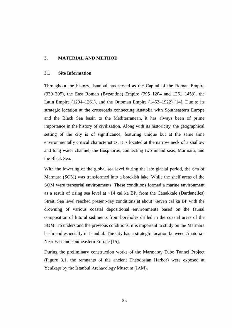
During the preliminary construction works of the Marmaray Tube Tunnel Project

(Figure 3.1, the remnants of the ancient Theodosian Harbor) were exposed at

Yenikapı by the İstanbul Archaeology Museum (IAM).

26

Figure 3.1 : Marmaray Project Plan and Profile [16].

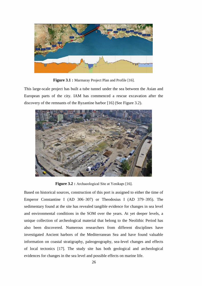
This large-scale project has built a tube tunnel under the sea between the Asian and

European parts of the city. IAM has commenced a rescue excavation after the

discovery of the remnants of the Byzantine harbor [16] (See Figure 3.2).

Figure 3.2 : Archaeological Site at Yenikapı [16].

Based on historical sources, construction of this port is assigned to either the time of

Emperor Constantine I (AD 306–307) or Theodosius I (AD 379–395). The

sedimentary found at the site has revealed tangible evidence for changes in sea level

and environmental conditions in the SOM over the years. At yet deeper levels, a

unique collection of archeological material that belong to the Neolithic Period has

also been discovered. Numerous researchers from different disciplines have

investigated Ancient harbors of the Mediterranean Sea and have found valuable

information on coastal stratigraphy, paleogeography, sea-level changes and effects

of local tectonics [17]. The study site has both geological and archeological

evidences for changes in the sea level and possible effects on marine life.

27

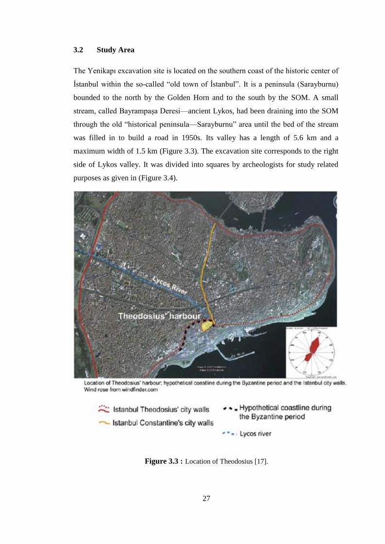
3.2 Study Area

The Yenikapı excavation site is located on the southern coast of the historic center of

İstanbul within the so-called “old town of İstanbul”. It is a peninsula (Sarayburnu)

bounded to the north by the Golden Horn and to the south by the SOM. A small

stream, called Bayrampaşa Deresi—ancient Lykos, had been draining into the SOM

through the old “historical peninsula—Sarayburnu” area until the bed of the stream

was filled in to build a road in 1950s. Its valley has a length of 5.6 km and a

maximum width of 1.5 km (Figure 3.3). The excavation site corresponds to the right

side of Lykos valley. It was divided into squares by archeologists for study related

purposes as given in (Figure 3.4).

Figure 3.3 : Location of Theodosius [17].

28

Figure 3.4 : The location of the excavation site in İstanbul. Digital image is produced from

Google Earth 4.3 [18].

The excavation site was divided into squares by archaelogisists for study related

purposes as given in Figure 3.5.

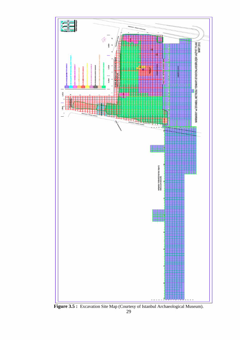
29 Figure 3.5 : Excavation Site Map (Courtesy of Istanbul Archaeological Museum).

30

3.3 Sample Properties

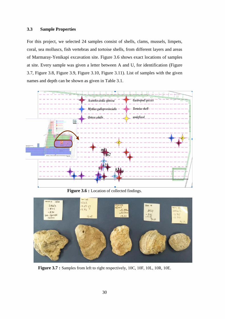
For this project, we selected 24 samples consist of shells, clams, mussels, limpets,

coral, sea molluscs, fish vertebras and tortoise shells, from different layers and areas

of Marmaray-Yenikapi excavation site. Figure 3.6 shows exact locations of samples

at site. Every sample was given a letter between A and U, for identification (Figure

3.7, Figure 3.8, Figure 3.9, Figure 3.10, Figure 3.11). List of samples with the given

names and depth can be shown as given in Table 3.1.

Figure 3.6 : Location of collected findings.

Figure 3.7 : Samples from left to right respectively, 10C, 10F, 10L, 10R, 10E.

31

Figure 3.8 : Samples from left to right respectively, 10K, 10P, 10I, 10Q, 10J.

Figure 3.9 : Samples from left to right respectively, 10Q, 10N, 10A, 10D.

Figure 3.10 : Samples from left to right respectively, 10H, 10M(1)(below),

10M(2)(above), 10B(1)(left), 10B(2)(right), 10G(right).

32

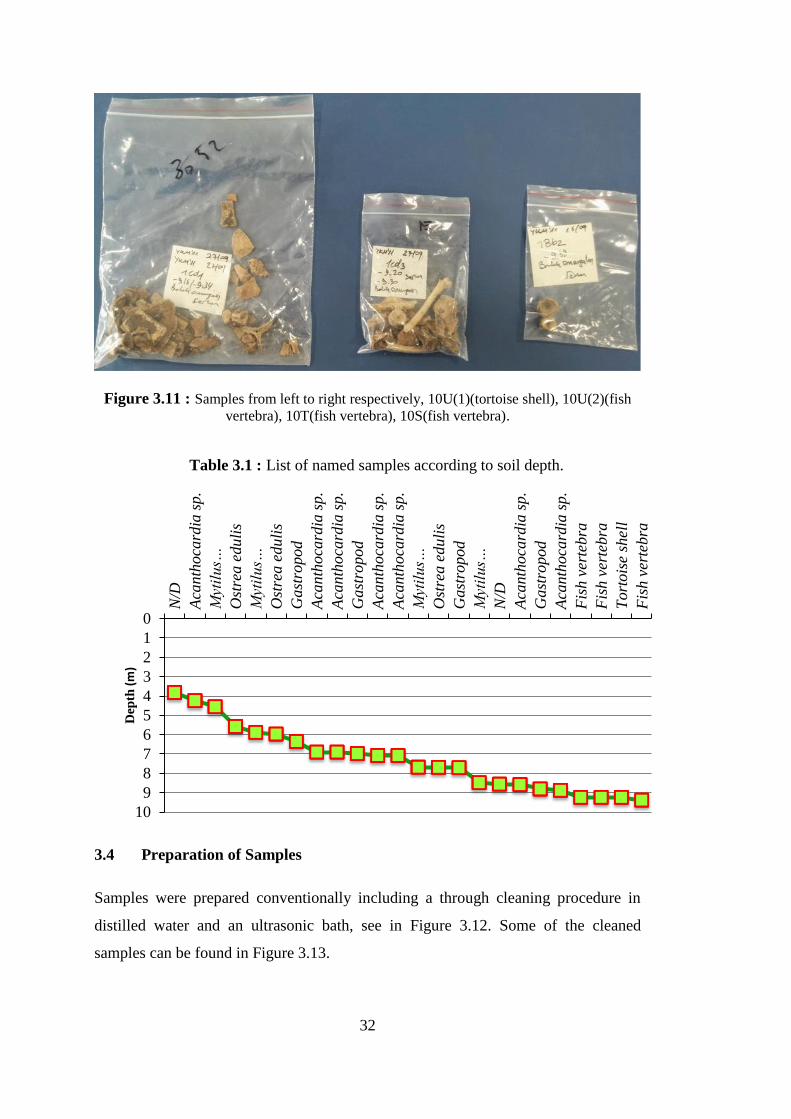
Figure 3.11 : Samples from left to right respectively, 10U(1)(tortoise shell), 10U(2)(fish

vertebra), 10T(fish vertebra), 10S(fish vertebra).

Table 3.1 : List of named samples according to soil depth.

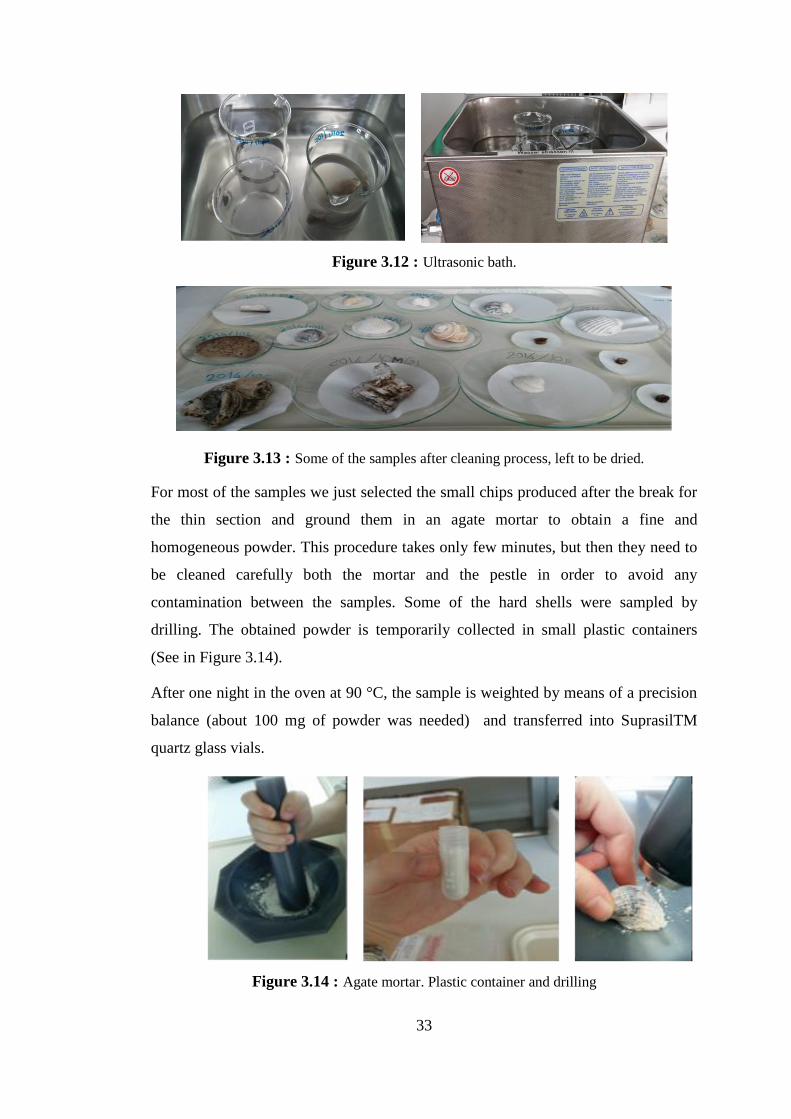
3.4 Preparation of Samples

Samples were prepared conventionally including a through cleaning procedure in

distilled water and an ultrasonic bath, see in Figure 3.12. Some of the cleaned

samples can be found in Figure 3.13.

0

1

2

3

4

5

6

7

8

9

10

N/D

Aca

nth

oca

rdia

sp.

Myt

ilus…

Ost

rea e

duli

s

Myt

ilus…

Ost

rea e

duli

s

Gast

ropod

Aca

nth

oca

rdia

sp.

Aca

nth

oca

rdia

sp.

Gast

ropod

Aca

nth

oca

rdia

sp.

Aca

nth

oca

rdia

sp.

Myt

ilus…

Ost

rea e

duli

s

Gast

ropod

Myt

ilus…

N/D

Aca

nth

oca

rdia

sp.

Gast

ropod

Aca

nth

oca

rdia

sp.

Fis

h v

erte

bra

Fis

h v

erte

bra

Tort

ois

e sh

ell

Fis

h v

erte

bra

Dep

th(m

)

33

Figure 3.12 : Ultrasonic bath.

Figure 3.13 : Some of the samples after cleaning process, left to be dried.

For most of the samples we just selected the small chips produced after the break for

the thin section and ground them in an agate mortar to obtain a fine and

homogeneous powder. This procedure takes only few minutes, but then they need to

be cleaned carefully both the mortar and the pestle in order to avoid any

contamination between the samples. Some of the hard shells were sampled by

drilling. The obtained powder is temporarily collected in small plastic containers

(See in Figure 3.14).

After one night in the oven at 90 °C, the sample is weighted by means of a precision

balance (about 100 mg of powder was needed) and transferred into SuprasilTM

quartz glass vials.

Figure 3.14 : Agate mortar. Plastic container and drilling

34

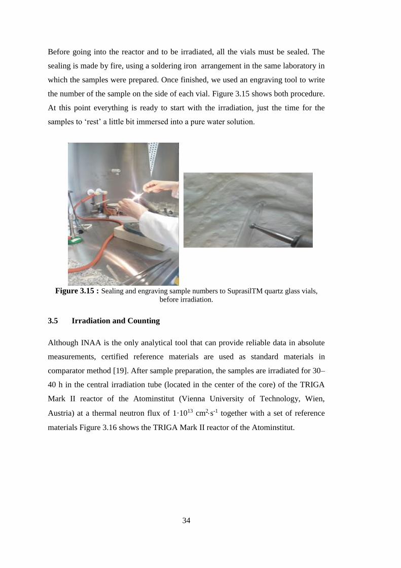
Before going into the reactor and to be irradiated, all the vials must be sealed. The

sealing is made by fire, using a soldering iron arrangement in the same laboratory in

which the samples were prepared. Once finished, we used an engraving tool to write

the number of the sample on the side of each vial. Figure 3.15 shows both procedure.

At this point everything is ready to start with the irradiation, just the time for the

samples to ‘rest’ a little bit immersed into a pure water solution.

Figure 3.15 : Sealing and engraving sample numbers to SuprasilTM quartz glass vials,

before irradiation.

3.5 Irradiation and Counting

Although INAA is the only analytical tool that can provide reliable data in absolute

measurements, certified reference materials are used as standard materials in

comparator method [19]. After sample preparation, the samples are irradiated for 30–

40 h in the central irradiation tube (located in the center of the core) of the TRIGA

Mark II reactor of the Atominstitut (Vienna University of Technology, Wien,

Austria) at a thermal neutron flux of 1·1013 cm2s-1 together with a set of reference

materials Figure 3.16 shows the TRIGA Mark II reactor of the Atominstitut.

35

Figure 3.16 : TRIGA Mark II reactor of the Atominstitut [20].

The amounts of elements in certified reference materials (Cl-Chondrit, Kruste85,

KrusteOben, KrusteGesamt, Bo-Norm, Shale, and BMSP) were given in Table 3.2,

Table 3.3 and Table 3.4 [21,22,23,24,25].

36

Table 3.2 : Essential element concentrations in used Standard Reference Materials (mg·kg-1).

Na K Cr Fe Co Ni Zn

Cl-Chondrit 5100 550 2650 181000 500 - 310

Kruste85 28300 25900 100 50000 25.00 - 70.00

KrusteOben 28900 28000 35 35000 10.00 - 71.00

KrusteGesamt 23000 9100 185 70700 29.00 - 80.00

Bo-Norm 33281 24287 1.973 21839 3.933 - 69.41

Shale 7803 31546 125 39565 25.70 1.00 1.00

BMSP 1010 21700 145 43400 9.37 - NA

37

Table 3.3 : Non-essential element concentrations in used Standard Reference Materials (mg·kg-1).

Sc As Rb Sr Zr Sb Cs Ba Hf Ta

Cl-Chondrit 5.92 1.850 2.300 - 3.820 0.140 0.190 2.410 0.103 0.014

Kruste85 22.00 1.800 90.00 - 165.0 0.20 3.00 425 3.000 2.000

KrusteOben 11.00 1.500 112.00 - 190.0 0.20 3.70 550 5.800 2.200

KrusteGesamt 30.00 1.000 32.00 - 100.0 0.20 1.00 250 3.000 1.000

Bo-Norm 8.58 2.773 108.23 - 289.7 0.30 2.89 564 7.747 0.804

Shale 14.90 28.40 125.00 300 200.0 2.09 5.16 636 6.300 1.120

BMSP 18.70 12.00 161.00 - NA 1.65 35.40 580 4.540 1.710

38

Table 3.4 : Lanthanide and actinide element concentrations in used Standard Reference Materials (mg·kg-1).

La Ce Nd Sm Eu Tb Yb Lu Th U

Cl-Chondrit 0.237 0.613 0.457 0.148 0.056 0.036 0.161 0.025 0.029 0.007

Kruste85 30.000 60.000 28.000 6.000 1.200 0.900 3.400 0.500 7.200 1.800

KrusteOben 30.000 64.000 26.000 4.500 0.880 0.640 2.200 0.320 10.700 2.800

KrusteGesamt 16.000 33.000 16.000 3.500 1.100 0.600 2.200 0.300 3.500 0.910

Bo-Norm 31.71 62.96 25.65 6.18 1.003 1.013 5.059 0.830 19.97 5.909

Shale 31.10 66.70 27.40 5.59 1.180 0.850 3.060 0.456 12.30 2.660

BMSP 50.50 106.20 NA 8.92 1.720 1.400 4.520 0.729 17.70 3.780

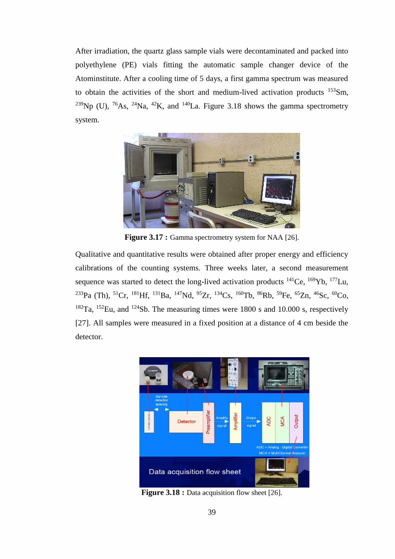
39

After irradiation, the quartz glass sample vials were decontaminated and packed into

polyethylene (PE) vials fitting the automatic sample changer device of the

Atominstitute. After a cooling time of 5 days, a first gamma spectrum was measured

to obtain the activities of the short and medium-lived activation products 153Sm,

239Np (U), 76As, 24Na, 42K, and 140La. Figure 3.18 shows the gamma spectrometry

system.

Figure 3.17 : Gamma spectrometry system for NAA [26].

Qualitative and quantitative results were obtained after proper energy and efficiency

calibrations of the counting systems. Three weeks later, a second measurement

sequence was started to detect the long-lived activation products 141Ce, 169Yb, 177Lu,

233Pa (Th), 51Cr, 181Hf, 131Ba, 147Nd, 95Zr, 134Cs, 160Tb, 86Rb, 59Fe, 65Zn, 46Sc, 60Co,

182Ta, 152Eu, and 124Sb. The measuring times were 1800 s and 10.000 s, respectively

[27]. All samples were measured in a fixed position at a distance of 4 cm beside the

detector.

Figure 3.18 : Data acquisition flow sheet [26].

40

The gamma-spectrometry was performed with a 151 cm3 HPGe-detector (1.8 keV

resolution at the 1332 keV 60Co peak; 50.1% relative efficiency), connected to a PC

based multi-channel analyser with a preloaded filter and a Loss-Free Counting

system. These analyses must be performed by means of short time activation

analysis, due to the short half-life of the respective activation products (see Table

3.5). Blank values of the quartz glass vials were measured and found negligible to

consider in calculations.

Table 3.5 Elements, activation products, half-lives, and γ-photon energies (sorted by

measurement sequences) [28].

Element Activation product Half-life (T1/2) γ-Energy

(keV)

(i) Short time activation analysis(if required)

Al 28Al 2.31 min 1778.8

Ca 49Ca 8.72 min 3084.4

Dy 165Dy 2.33 h 94.7

Mn 56Mn 2.58 h 1811.2

Ti 51Ti 5.79 min 320

V 52V 3.75 min 1434.2

(ii) Measurement 5 days after neutron irradiation

As 76As 25.87 h 559.1

K 42K 12.36 h 1524.7

La 140La 40.26 h 1596.2

Lu 177Lu 6.65 d 208.4

Na 24Na 14.96 h 1368.6;

2754.1

Sm 153Sm 46.28 h 103.2

U 239Np 56.55 h 277.6

41

Table 3.5 (continued) Elements, activation products, half-lives, and γ-photon

energies (sorted by measurement sequences) [28].

Element Activation

product Half-life (T1/2)

γ-Energy

(keV)

(iv) Measurement 28 days after neutron irradiation

Ba 131Ba 11.5 d 496.3

Ce 141Ce 32.5 d 145.5

Co 60Co 5.27 a 1173.2

Cr 51Cr 27.7 d 320.1

Cs 134Cs 2.07 a 795.8

Eu 152Eu 13.52 a 1408.1

Fe 59Fe 44.5 d 1099.2

Hf 181Hf 42.39 d 482.2

Lu 177Lu 6.65 d 208.4

Nd 147Nd 10.98 d 531

Rb 86Rb 18.64 d 1076.6

Sb 124Sb 60.2 d 1691

Sc 46Sc 83.79 d 1120.5

Ta 182Ta 114.43d 1221.3;

1189.1

Tb 160Tb 72.3 d 879.4

Th 233Pa 26.96 d 311.9

Yb 169Yb 32.02 d 177.2

Zn 65Zn 244.06d 1115.5

Zr 95Zr 64.03 d 756.7

In Table 3.5 239Np is the decay product of 239U (T1/2 = 23.5 min), which is the

activation product of 238U, and can be detected more sensitively. 233Pa is the decay

product of 233Th (T1/2 = 22.3 min), which is the activation product of 232Th, and can

be detected more sensitively.

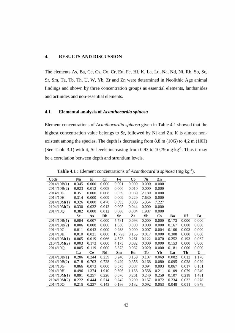
43

4. RESULTS AND DISCUSSION

The elements As, Ba, Ce, Cs, Co, Cr, Eu, Fe, Hf, K, La, Lu, Na, Nd, Ni, Rb, Sb, Sc,

Sr, Sm, Ta, Tb, Th, U, W, Yb, Zr and Zn were determined in Neolithic Age animal

findings and shown by three concentration groups as essential elements, lanthanides

and actinides and non-essential elements.

4.1 Elemental analysis of Acanthocardia spinosa

Element concentrations of Acanthocardia spinosa given in Table 4.1 showed that the

highest concentration value belongs to Sr, followed by Ni and Zn. K is almost non-

existent among the species. The depth is decreasing from 8,8 m (10G) to 4,2 m (10H)

(See Table 3.1) with it, Sr levels increasing from 0.93 to 10,79 mgkg-1. Thus it may

be a correlation between depth and strontium levels.

Table 4.1 : Element concentrations of Acanthocardia spinosa (mgkg-1).

Code Na K Cr Fe Co Ni Zn

2014/10B(1) 0.345 0.000 0.000 0.001 0.009 0.000 0.000

2014/10B(2) 0.023 0.012 0.008 0.006 0.010 0.000 0.000

2014/10G 0.351 0.000 0.008 0.039 0.039 2.180 0.000

2014/10H 0.314 0.000 0.009 0.009 0.229 7.630 0.000

2014/10M(1) 0.326 0.000 0.470 0.095 0.093 5.354 7.227

2104/10M(2) 0.330 0.032 0.012 0.005 0.044 0.000 0.000

2014/10Q 0.382 0.000 0.012 0.006 0.084 1.987 0.000


2014/10B(1) 0.004 0.007 0.000 5.781 0.098 0.000 0.000 0.173 0.000 0.000

2014/10B(2) 0.006 0.008 0.000 1.630 0.000 0.000 0.000 0.167 0.000 0.000

2014/10G 0.011 0.043 0.000 0.938 0.000 0.007 0.004 0.100 0.003 0.000

2014/10H 0.010 0.021 0.000 10.793 0.155 0.017 0.000 0.308 0.000 0.000

2014/10M(1) 0.065 0.019 0.066 4.573 0.261 0.122 0.070 0.252 0.193 0.067

2104/10M(2) 0.003 0.173 0.000 4.175 0.082 0.000 0.000 0.153 0.000 0.000

2014/10Q 0.005 0.119 0.000 6.373 0.062 0.020 0.000 0.181 0.000 0.000


2014/10B(1) 0.286 0.244 0.239 0.240 0.159 0.107 0.069 0.082 0.012 1.176

2014/10B(2) 0.718 0.703 0.728 0.429 0.356 0.168 0.080 0.095 0.028 0.029

2014/10G 0.866 0.073 0.000 0.575 0.087 0.094 0.093 0.067 0.017 0.181

2014/10H 0.496 1.374 1.910 0.396 1.158 0.558 0.211 0.109 0.079 0.249

2014/10M(1) 0.891 0.257 0.226 0.676 0.261 0.240 0.259 0.107 0.218 1.481

2104/10M(2) 0.222 0.444 0.514 0.242 0.299 0.157 0.072 0.234 0.032 0.278

2014/10Q 0.215 0.237 0.143 0.186 0.132 0.092 0.053 0.048 0.011 0.878

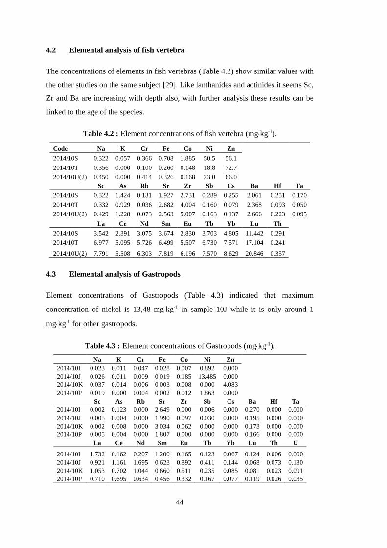
44

4.2 Elemental analysis of fish vertebra

The concentrations of elements in fish vertebras (Table 4.2) show similar values with

the other studies on the same subject [29]. Like lanthanides and actinides it seems Sc,

Zr and Ba are increasing with depth also, with further analysis these results can be

linked to the age of the species.

Table 4.2 : Element concentrations of fish vertebra (mgkg-1).

Code Na K Cr Fe Co Ni Zn

2014/10S 0.322 0.057 0.366 0.708 1.885 50.5 56.1

2014/10T 0.356 0.000 0.100 0.260 0.148 18.8 72.7

2014/10U(2) 0.450 0.000 0.414 0.326 0.168 23.0 66.0


2014/10S 0.322 1.424 0.131 1.927 2.731 0.289 0.255 2.061 0.251 0.170

2014/10T 0.332 0.929 0.036 2.682 4.004 0.160 0.079 2.368 0.093 0.050

2014/10U(2) 0.429 1.228 0.073 2.563 5.007 0.163 0.137 2.666 0.223 0.095

La Ce Nd Sm Eu Tb Yb Lu Th

2014/10S 3.542 2.391 3.075 3.674 2.830 3.703 4.805 11.442 0.291

2014/10T 6.977 5.095 5.726 6.499 5.507 6.730 7.571 17.104 0.241

2014/10U(2) 7.791 5.508 6.303 7.819 6.196 7.570 8.629 20.846 0.357

4.3 Elemental analysis of Gastropods

Element concentrations of Gastropods (Table 4.3) indicated that maximum

concentration of nickel is 13,48 mgkg-1 in sample 10J while it is only around 1

mgkg-1 for other gastropods.

Table 4.3 : Element concentrations of Gastropods (mgkg-1).

Na K Cr Fe Co Ni Zn

2014/10I 0.023 0.011 0.047 0.028 0.007 0.892 0.000

2014/10J 0.026 0.011 0.009 0.019 0.185 13.485 0.000

2014/10K 0.037 0.014 0.006 0.003 0.008 0.000 4.083

2014/10P 0.019 0.000 0.004 0.002 0.012 1.863 0.000


2014/10I 0.002 0.123 0.000 2.649 0.000 0.006 0.000 0.270 0.000 0.000

2014/10J 0.005 0.004 0.000 1.990 0.097 0.030 0.000 0.195 0.000 0.000

2014/10K 0.002 0.008 0.000 3.034 0.062 0.000 0.000 0.173 0.000 0.000

2014/10P 0.005 0.004 0.000 1.807 0.000 0.000 0.000 0.166 0.000 0.000


2014/10I 1.732 0.162 0.207 1.200 0.165 0.123 0.067 0.124 0.006 0.000

2014/10J 0.921 1.161 1.695 0.623 0.892 0.411 0.144 0.068 0.073 0.130

2014/10K 1.053 0.702 1.044 0.660 0.511 0.235 0.085 0.081 0.023 0.091

2014/10P 0.710 0.695 0.634 0.456 0.332 0.167 0.077 0.119 0.026 0.035

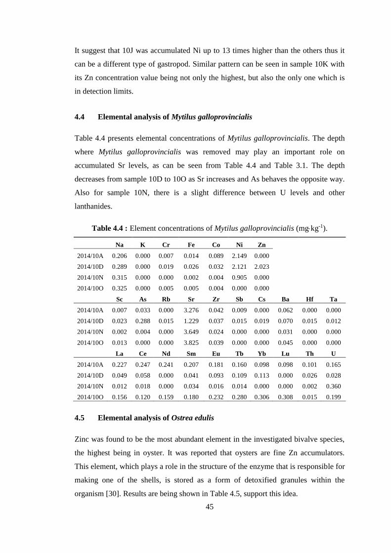
45

It suggest that 10J was accumulated Ni up to 13 times higher than the others thus it

can be a different type of gastropod. Similar pattern can be seen in sample 10K with

its Zn concentration value being not only the highest, but also the only one which is

in detection limits.

4.4 Elemental analysis of Mytilus galloprovincialis

Table 4.4 presents elemental concentrations of Mytilus galloprovincialis. The depth

where Mytilus galloprovincialis was removed may play an important role on

accumulated Sr levels, as can be seen from Table 4.4 and Table 3.1. The depth

decreases from sample 10D to 10O as Sr increases and As behaves the opposite way.

Also for sample 10N, there is a slight difference between U levels and other

lanthanides.

Table 4.4 : Element concentrations of Mytilus galloprovincialis (mgkg-1).

Na K Cr Fe Co Ni Zn

2014/10A 0.206 0.000 0.007 0.014 0.089 2.149 0.000

2014/10D 0.289 0.000 0.019 0.026 0.032 2.121 2.023

2014/10N 0.315 0.000 0.000 0.002 0.004 0.905 0.000

2014/10O 0.325 0.000 0.005 0.005 0.004 0.000 0.000


2014/10A 0.007 0.033 0.000 3.276 0.042 0.009 0.000 0.062 0.000 0.000

2014/10D 0.023 0.288 0.015 1.229 0.037 0.015 0.019 0.070 0.015 0.012

2014/10N 0.002 0.004 0.000 3.649 0.024 0.000 0.000 0.031 0.000 0.000

2014/10O 0.013 0.000 0.000 3.825 0.039 0.000 0.000 0.045 0.000 0.000


2014/10A 0.227 0.247 0.241 0.207 0.181 0.160 0.098 0.098 0.101 0.165

2014/10D 0.049 0.058 0.000 0.041 0.093 0.109 0.113 0.000 0.026 0.028

2014/10N 0.012 0.018 0.000 0.034 0.016 0.014 0.000 0.000 0.002 0.360

2014/10O 0.156 0.120 0.159 0.180 0.232 0.280 0.306 0.308 0.015 0.199

4.5 Elemental analysis of Ostrea edulis

Zinc was found to be the most abundant element in the investigated bivalve species,

the highest being in oyster. It was reported that oysters are fine Zn accumulators.

This element, which plays a role in the structure of the enzyme that is responsible for

making one of the shells, is stored as a form of detoxified granules within the

organism [30]. Results are being shown in Table 4.5, support this idea.

46

Table 4.5 : Element concentrations of Ostrea edulis (mgkg-1).

Na K Cr Fe Co Ni Zn

2014/10F 0.113 0.000 0.442 0.080 0.099 5.629 5.648

2014/10L 0.375 0.051 0.005 0.007 0.044 3.300 3.430

2014/10R 0.311 0.000 0.702 0.028 0.060 4.143 2.032


2014/10F 0.046 0.051 0.068 1.540 0.259 0.066 0.054 0.143 0.175 0.063

2014/10L 0.002 0.207 0.000 1.779 0.049 0.000 0.000 0.102 0.000 0.000

2014/10R 0.009 0.189 0.000 2.938 0.164 0.036 0.004 1.600 0.152 0.018


2014/10F 0.061 0.204 0.217 0.092 0.276 0.260 0.234 0.105 0.084 0.268

2014/10L 0.168 0.777 0.936 0.192 0.507 0.235 0.089 0.154 0.057 0.302

2014/10R 0.056 0.061 0.000 0.060 0.033 0.035 0.034 0.046 0.054 0.088

4.6 Elemental analysis of tortoise shell

Tortoise shells are composed of bone, and an incrementally grown covering of

keratinized tissue (scutes) that can function as a repository for certain

bioaccumulated trace elements. Since hard keratinized tissues of this type are

virtually isolated from other metabolic activity, resident elemental species have

limited mobility [12]. It is reasonable to assume therefore, that the grown shell of the

tortoise represent a relatively stable elemental uptake. As shown in Table 4.6 most

abundant elements in shell are Ni, Zn, and Lu. Similar results were obtained by fish

vertebras (see also Table 4.2) consistent with its bone like chemical composition thus

it may be evaluated alongside with fish vertebras.

Table 4.6 : Element concentrations of tortoise shell (mgkg-1).

Na K Cr Fe Co Ni Zn 2014/10U(1) 0.217 0.000 0.080 1.070 0.820 30.56 52.89


2014/10U(1) 0.154 0.341 0.009 1.671 3.298 0.228 0.039 1.919 0.047 0.023


2014/10U(1) 4.42 3.50 3.63 4.79 3.51 4.44 5.28 14.26 0.09

4.7 Elemental analysis of non determined species

By comparing element concentration in Table 4.7 with the data obtained from the

study it can be found a correlation between other species. In fact the element

distributions are not only similar thoroughout the two samples, it is almost exactly

proportional with from the Acanthocardia spinosa familia, namely 10M(2) (See

Table 4.1 and Figure 4.1).

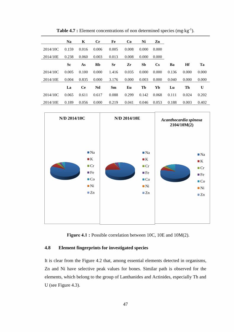
47

Table 4.7 : Element concentrations of non determined species (mgkg-1).

Na K Cr Fe Co Ni Zn

2014/10C 0.159 0.016 0.006 0.005 0.008 0.000 0.000

2014/10E 0.238 0.060 0.003 0.013 0.008 0.000 0.000


2014/10C 0.005 0.100 0.000 1.416 0.035 0.000 0.000 0.136 0.000 0.000

2014/10E 0.004 0.835 0.000 3.176 0.000 0.003 0.000 0.040 0.000 0.000


2014/10C 0.065 0.611 0.617 0.088 0.299 0.142 0.068 0.111 0.024 0.202

2014/10E 0.189 0.056 0.000 0.219 0.041 0.046 0.053 0.188 0.003 0.402

Possible correlation between 10C, 10E and 10M(2).

4.8 Element fingerprints for investigated species

It is clear from the Figure 4.2 that, among essential elements detected in organisms,

Zn and Ni have selective peak values for bones. Similar path is observed for the

elements, which belong to the group of Lanthanides and Actinides, especially Th and

U (see Figure 4.3).

N/D 2014/10C

Na

K

Cr

Fe

Co

Ni

Zn

N/D 2014/10E

Na

K

Cr

Fe

Co

Ni

Zn

Acanthocardia spinosa

2104/10M(2)

Na

K

Cr

Fe

Co

Ni

Zn

48

Essential element distribution in samples according to average

concentration values between species.

Lanthanides and actinides element distribution in samples according

to average concentration values between species.

As seen from Figure 4.4, Sr and Ba increase distinctly throughout species and can be

further discussed regarding its function in living organisms or forming shells.

Na

Cr

Co

Zn

010

20

30

40

50

60

70

Na

K

Cr

Fe

Co

Ni

Zn

0

5

10

15

20


Acanthocardia spinosa

Gastropod

Mytilus galloprovincialis

N/D

Ostrea edulis

Fish vertebra

Tortoise shell

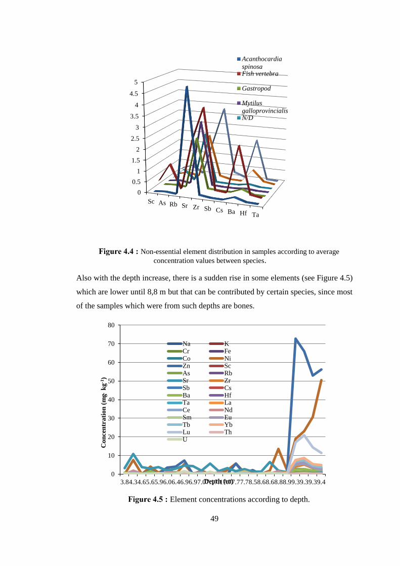
49

Non-essential element distribution in samples according to average

concentration values between species.

Also with the depth increase, there is a sudden rise in some elements (see Figure 4.5)

which are lower until 8,8 m but that can be contributed by certain species, since most

of the samples which were from such depths are bones.

Element concentrations according to depth.

0

0.5

1

1.5

2

2.5

3

3.5

4

4.5

5


Acanthocardia

spinosaFish vertebra

Gastropod

Mytilus

galloprovincialisN/D

0

10

20

30

40

50

60

70

80

3.84.34.65.65.96.06.46.96.97.07.17.17.77.77.78.58.68.68.88.99.39.39.39.4

Co

nce

ntr

ati

on

(m

g

kg

-1)

Depth (m)

Na KCr FeCo NiZn ScAs RbSr ZrSb CsBa HfTa LaCe NdSm EuTb YbLu ThU

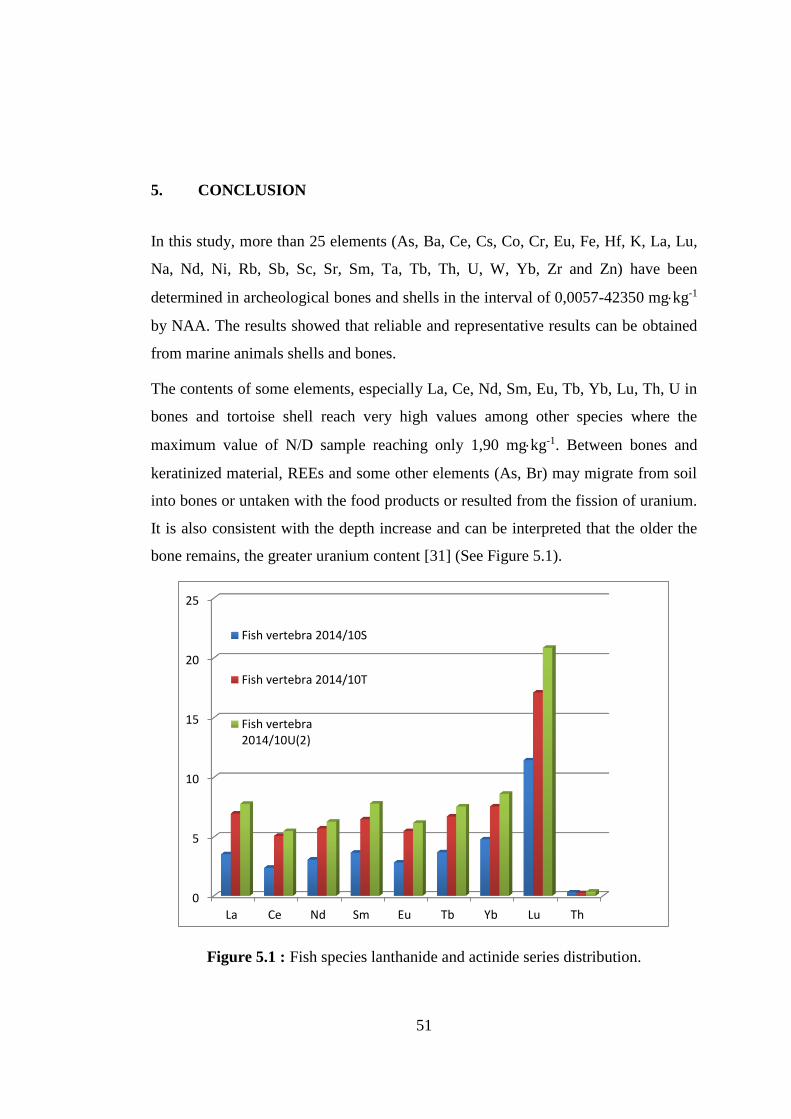
51

5. CONCLUSION

In this study, more than 25 elements (As, Ba, Ce, Cs, Co, Cr, Eu, Fe, Hf, K, La, Lu,

Na, Nd, Ni, Rb, Sb, Sc, Sr, Sm, Ta, Tb, Th, U, W, Yb, Zr and Zn) have been

determined in archeological bones and shells in the interval of 0,0057-42350 mgkg-1

by NAA. The results showed that reliable and representative results can be obtained

from marine animals shells and bones.

The contents of some elements, especially La, Ce, Nd, Sm, Eu, Tb, Yb, Lu, Th, U in

bones and tortoise shell reach very high values among other species where the

maximum value of N/D sample reaching only 1,90 mgkg-1. Between bones and

keratinized material, REEs and some other elements (As, Br) may migrate from soil

into bones or untaken with the food products or resulted from the fission of uranium.

It is also consistent with the depth increase and can be interpreted that the older the

bone remains, the greater uranium content [31] (See Figure 5.1).

Figure 5.1 : Fish species lanthanide and actinide series distribution.

0

5

10

15

20

25


Fish vertebra 2014/10S

Fish vertebra 2014/10T

Fish vertebra2014/10U(2)

52

According to Chang et al. trace metal concentrations in shells of mollusk species

vary to a wide range even if they belong to the same taxon. The differences between

different species from different regions may be attributable to influential factors that

govern the incorporation of trace metals during molluscan shell formation.

These influential factors can be summarized as differences in (a) taxonomies and

ontogenetic stages, (b) mineralogy (biomineralization) of the shell, and (c) salinity

and temperature of different water environments [32].

For bivalves it is known that the strength of the net accumulation patterns of metals

vary both between metals but also, for one metal between species or more

significantly between higher taxa such as families, correlating with their metal

physiology including their ability to excrete or store particular trace elements. These

factors explain the variation between, for example, the very high zinc concentrations

in oysters (Ostreidae) and the much lower zinc concentrations in mussels (Mytilidae)

[33] (See Figure 5.2).

Figure 5.2 : Zn concentrations for Mytilus g. and Ostrea e. species (mgkg-1).

Such variation is expected in the Bivalvia where there are consistent differences in

metal accumulation patterns between families including mytilids, ostreids, pectinids

and venerids.

0

0.5

1

1.5

2

2.5

3

3.5

4

Aver

age

Zn c

once

ntr

atio

n (

mgk

g-1

)

Mytilus

galloprovincialis

Ostrea edulis

53

To conclude we can say considering that the organisms are the most active and

deterministic factors of the environment, data obtained in this study will serve as a

database for future studies.

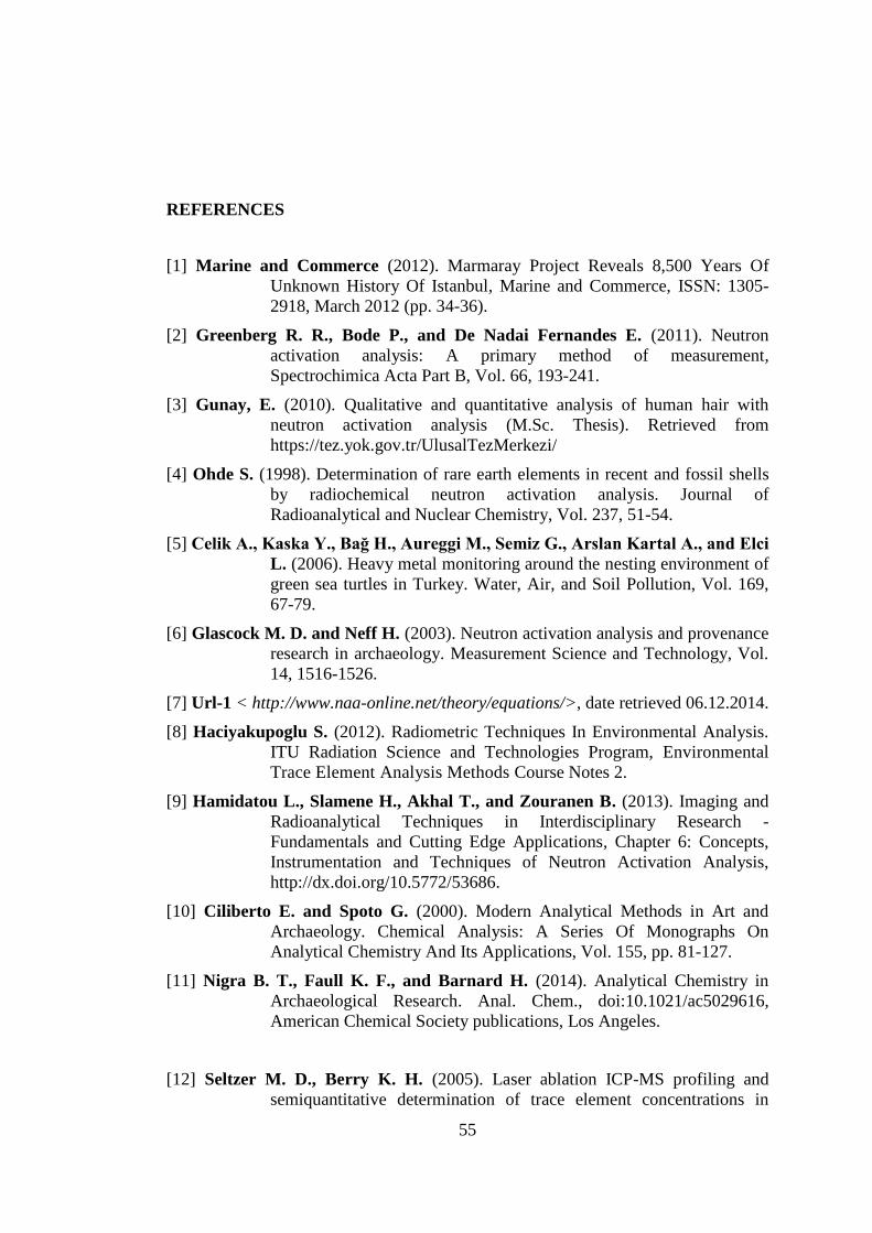
55

REFERENCES

[1] Marine and Commerce (2012). Marmaray Project Reveals 8,500 Years Of

Unknown History Of Istanbul, Marine and Commerce, ISSN: 1305-

2918, March 2012 (pp. 34-36).

[2] Greenberg R. R., Bode P., and De Nadai Fernandes E. (2011). Neutron

activation analysis: A primary method of measurement,

Spectrochimica Acta Part B, Vol. 66, 193-241.

[3] Gunay, E. (2010). Qualitative and quantitative analysis of human hair with

neutron activation analysis (M.Sc. Thesis). Retrieved from

https://tez.yok.gov.tr/UlusalTezMerkezi/

[4] Ohde S. (1998). Determination of rare earth elements in recent and fossil shells

by radiochemical neutron activation analysis. Journal of

Radioanalytical and Nuclear Chemistry, Vol. 237, 51-54.

[5] Celik A., Kaska Y., Bağ H., Aureggi M., Semiz G., Arslan Kartal A., and Elci

L. (2006). Heavy metal monitoring around the nesting environment of

green sea turtles in Turkey. Water, Air, and Soil Pollution, Vol. 169,

67-79.

[6] Glascock M. D. and Neff H. (2003). Neutron activation analysis and provenance

research in archaeology. Measurement Science and Technology, Vol.

14, 1516-1526.

[7] Url-1 < http://www.naa-online.net/theory/equations/>, date retrieved 06.12.2014.

[8] Haciyakupoglu S. (2012). Radiometric Techniques In Environmental Analysis.

ITU Radiation Science and Technologies Program, Environmental

Trace Element Analysis Methods Course Notes 2.

[9] Hamidatou L., Slamene H., Akhal T., and Zouranen B. (2013). Imaging and

Radioanalytical Techniques in Interdisciplinary Research -

Fundamentals and Cutting Edge Applications, Chapter 6: Concepts,

Instrumentation and Techniques of Neutron Activation Analysis,

http://dx.doi.org/10.5772/53686.

[10] Ciliberto E. and Spoto G. (2000). Modern Analytical Methods in Art and

Archaeology. Chemical Analysis: A Series Of Monographs On

Analytical Chemistry And Its Applications, Vol. 155, pp. 81-127.

[11] Nigra B. T., Faull K. F., and Barnard H. (2014). Analytical Chemistry in

Archaeological Research. Anal. Chem., doi:10.1021/ac5029616,

American Chemical Society publications, Los Angeles.

[12] Seltzer M. D., Berry K. H. (2005). Laser ablation ICP-MS profiling and

semiquantitative determination of trace element concentrations in

56

desert tortoise shells: documenting the uptake of elemental toxicants.

Science of the Total Environment, Vol. 339, 253-265.

[13] Nadkarni R. A. and Morrison G. H. (1973). Multi element Instrumental

Neutron Activation Analysis of Biological Materials. Analytical

Chemistry, Vol. 45, No. 11 1957-1960.

[14] Url-4 < http://www2.kenes.com/stroke2014/info/Pages/AboutIstanbul.aspx>,

date retrieved 09.03.2015.

[15] Yalcin M. N., Algan O., Ozdogan M., Yilmaz I., Sari E., Kirci-Elmas E.,

Bulkan O., Ongan D., Gazioglu C., Yilmaz Y., Nazik A., Polat M.

A., and Meric E. (2011). Holocene coastal change in the ancient

harbor of Yenikapı–İstanbul and its impact on cultural history,

Quaternary Research, Vol. 76, 30-45.

[16] Buket Z., Belkaya H., Ozmen I. H., and Karamut I. (2012). The Marmaray

Project: Taking Good Care of the Natural Environment And The

Historical Heritage Of Istanbul,

http://www.ctta.org/fileupload/ita/2009/papers/p-10/p-10-03.pdf

[17] Bony G., Marriner N., Morhange C., Kaniewski D., and Perinçek D. (2012).

A high-energy deposit in the Byzantine harbour of Yenikapı, Istanbul

(Turkey), Quaternary International, Vol. 266, 117-130.

[18] Algan O., Yalcin M. N., Ozdogan M., Yilmaz I., Sari E., Kirci-Elmas E.,

Ongan D., Bulkan-Yesiladalı B., Yilmaz Y., and Karamut I. (2009). A short note on the geo-archeological significance of the

ancient Theodosius harbor (İstanbul, Turkey), Quaternary Research,

Vol. 72, 457-461.

[19] Landmann G., Kempe S., Bichler M., Steinhauser, G., and Sterba H. J.

(2011). Geochemical fingerprints by activation analysis of tephra

layers in Lake Van sediments, Turkey. Applied Radiation and

Isotopes, Vol. 69, 929-935.

[20] Url-2 <

http://www.tuwien.ac.at/dle/pr/aktuelles/downloads/2010/zehntausend

ster_betriebstag_des_forschungsreaktors_am_atominstitut/>, date

retrieved 12.12.2014.

[21] Taylor Ross S., and McLennan M. S., (1985). The Continental Crust: its

Composition and Evolution, Blackwell Scientific Publications

[22] Taylor S. R. (1964). Abundance of chemical elements in the continental crust: a

new table, Geochimica et Cosmochimica Acta, Vol. 28, 1273-1285.

[23] Gromet L. P., Dymek R. F., Korotev R. L., and Haskin L. A. (1984). The

‘’North American shale composite’’: Its compilation major and trace

element characteristics, Geochimica et Cosmochimica Acta, Vol. 48,

2469-2482.

[24] Potts P. J. and Whitley J. E. (1976). Determination and Interpretation of Rare-

earth Abundances in Rocks and Minerals, Proc. Analysis Division

Chem. Soc., 118-121

57

[25] Peltz C., Schmid P., and Bichler M. (1999). INAA of Aegaen pumices for the

classification of archaeological findings, Journal of Radioanalytical

and Nuclear Chemistry, Vol. 243, No. 2, 361-377.

[26] Url-3 <

http://serc.carleton.edu/research_education/geochemsheets/technique

s/INAA.html>, date retrieved 12.12.2014.

[27] Bichler M., Steinhauser, G., and Sterba H. J. (2007). ‘‘Chemical

fingerprints’’ of pumice from Cappadocia (Turkey) and Kos (Greece)

for archaeological applications. Applied Radiation and Isotopes, Vol.

65, 488-503.

[28] Steinhauser, G., Sterba H. J., Bichler M., and Huber H. (2006). Neutron

activation analysis of Mediterranean volcanic rocks– An analytical

database for archaeological stratigraphy. Applied Geochemistry, Vol.

21, 1362-1375.

[29] Yamada M., Fujimori K., Yamada G., Moriwake Y., Tohno S., and Tohno

Y. (2001). Trace Metals in Vertebral Columns of Deep-Sea Teleost

Fish. Biological Trace Element Research, Vol. 80, 245-249.

[30] Colakoglu S., Ulukoy G., Ormanci H.B., and Colakoglu F. A. (2012). Metal

levels in economically important bivalve species from Turkey, Food

Additives & Contaminants: Part B: Surveillance, 5:4, 272-278, DOI:

10.1080/19393210.2012.707233

[31] Vasidov A., Osinskaya N. S., Khatamov Sh., Rakhmanova T., and

Akhmadshaev A. Sh. (2008). Instrumental neutron activation

analysis of prehistoric and ancient bone remains. Journal of

Radioanalytical and Nuclear Chemistry, Vol. 278, No.2, 287-291.

[32] Pourang N., Richardson C. A., Chenery S. R. N. and Nasrollahzedeh H.

(2014). Assessment of trace elements in the shell layers and soft

tissues of the pearl oyster Pinctada radiata using multivariate analyses:

a potential proxy for temporal and spatial variations of trace elements.

Environmental Monitoring Assessment, Vol. 186, 2465-2485.

[33] Marsden I. D., Smith B. D., Rainbowb P. S. (2014). Effects of environmental

and physiological variables on the accumulated concentrations of trace

metals in the New Zealand cockle Austrovenus stutchburyi. Science of

the Total Environment Vol. 470–471, 324–339.

59

CURRICULUM VITAE

Name Surname: Ayşe Tuba ÖNGÜL

Place and Date of Birth: Istanbul 12.02.1987

Address: Çaldıran Sk. Akmara Apt. 16/10

Bahçelievler/Istanbul

E-Mail: [email protected]

B.Sc.: Yildiz Technical University – Physics 2011

ISTANBUL TECHNICAL UNIVERSITY ENERGY INSTITUTE

Documents

Transcript of ISTANBUL TECHNICAL UNIVERSITY ENERGY INSTITUTE