ISSN:2664-5564 (print) Vol 11.2( April 2021) ...

University of Thi_Qar Journal for Engineering Sciences ISSN :2664- 5572 ( online)

http://www.doi.org/10.31663/tqujes.11.2.395(2021) ISSN:2664-5564 (print)

http://jeng.utq.edu.iqle at Availab Vol 11.2( April 2021)

utjeng@ utq.edu.iq

72

Evaluation of Line Power Losses under Variable Power Supplied by Wind Generation and PV

Attached at Different Bus-bars

Mustafa Jameel†, Ali Salam Kadhim

‡

†Department of Electrical and Electronics Engineering, University of Thi-Qar, Thi-Qar, Iraq, Email.

‡ Department of Electrical and Electronics Engineering, University of Thi-Qar, Thi-Qar, Iraq, ali-al-

[email protected].

Abstract

The aim of this paper is to solve the load flow for Power System Connection (IEEE 6 Bus System),

and find the power losses in the transmission lines and the total power losses for 10 MVA base

power rating and 33 KV rated voltage. This can be achieved with the aids of simulation by using a

software programme called PSAT, which is compatible with MATLAB. In addition, to improve the

efficiency of the system a 2 MW wind turbine has to be installed on the system, but due to the fact

that the wind turbine has changeable output power and this leads to variation in the voltages and

currents in the transmission system. Therefore, we will examine the effect of the 2 MW wind turbine

at different busbars and find out where is the optimal location for the turbine, which results in low

system losses and optimum voltage. The next section is to apply a PV generator with variable output

on different busbars and find the best position that we can obtain less power losses and optimum

voltage regulation. The final section is to apply 0.5 PV generators at different buses at the same time

and compare the result with the case obtained from applying 2 MW PV generators.

Keywords: Load flow, Power losses, PSAT, Wind turbine, Optimum voltage.

1. Introduction

Active and Reactive power in all three phase AC

power system are flowing from the generation

station where the AC power is generated to the

load where it is consumed via many buses and

transmission lines branches. Studying power

flow from generation station to the load called

load flow studies or power flow studies, such

type of studies are in the category of the steady

state analysis for the operation condition of a

power system, and their aim is to calculate the

voltages, phase angle, real and reactive power

flows through the system for a specific load

condition. Moreover, in these studies we make

an assumption either for the value of the bus

voltages or for the power, which has been

supplied to the bus. The purpose of the power

flow analysis is to provide the consumer with the

power that needs in real time and with suitable

limits for the voltages and frequency. In

addition, to anticipate ahead and take into

account for any situation that could happen in

the system. Such as, if one of the transmission

lines is to be taken off for the purpose of

maintenance, are the other lines in the system

can manage the required load without override

their rated values.

Fig.1 Power System Connection (IEEE 6 Bus

System)

The bus in the power system is accompanying

with four different quantities named as voltage

magnitude, voltage phase, real or active power

and reactive power. In the procedure of solution

the load flow studies, two of those quantities are

http://jeng.utq.edu.iq/

mailto:[email protected]

Mustafa Jameel, Ali Salam Evaluation of Line Power Losses under Variable Power Supplies by

Wind generation and PV Attached at Different Bus-bars

73

known and the rest should be found. According

to those four quantities, the buses in the power

system are classified into the following types:

1. Slack bus: Also, called swing bus and it acts

as the reference generator for the power

system and its voltage magnitude is (1 per

unit) and the phase of the voltage is assumed

to be zero ∠0. In the slack bus, the active

power P and reactive power Q generated is

unknown and can be found through the load

flow solution.

2. Load bus: Also, called P & Q bus, therefore

active and reactive power are known , and

the voltage magnitude and phase have to be

found from the load flow solution. In this

bus, no generator is connected to it.

3. Generator bus: Also, called voltage

controlled bus and in this bus the magnitude

of the voltages is kept constant and this can

be achieved by adjusting the field current of

the generator. The real power generation for

each generator in this bus is assigned. In this

bus the reactive power and the phase of the

voltage is unknown.

Many methods can be used to solve the load

flow problems such as Gauss-Seidal method and

Newton-Raphson (NR) methods, which are

based on the iterative technique. Moreover, the

programme PSAT uses Newton-Raphson

technique to solve problems of load flow in large

power network [1,2,3].

The Newton-Raphson method as mentioned in

many references is the most computationally

efficient and common way used for calculation

of load flow. This is because of its several

advantages. The convergence characteristics for

example of NR are not affected by the choice of

a slack bus, while this selection has noticeable

effects in Gauss-Siedal. These effects can

basically result in poor convergence. In addition,

NR approach is very suitable for the large

networks because the requirement for the

computer storage is reasonable and increase

linearly with the problem size. Furthermore, The

NR method has a great flexibility, so it allows

for a very wide range of requirements, such as,

onload-tap changing and phase-shift devices,

remote voltage control and functional loads, to

be included efficiently. Thus, NR method is

crucial for many novel developed techniques,

which are required for obtaining the premium

operation of a power system, system-state

evaluation, analysis accuracy, modeling of linear

network and the analysis of transient-stability[4].

2. Voltage Regulation

Voltage regulation of the transmission line is a

measure of change in the magnitude of the

voltage between the sending and receiving end.

There are two different types of voltage

regulation and this difference depends on the

reference voltage:

1. Regulation down: this is the change in

the terminal voltage when the full load

current for any given power factor is

applied, and it is expressed as a fraction

of no-load terminal voltage. This kind of

regulation is normally used in the

transformer.

Regulation voltage = |𝑉𝑛𝑙|−|𝑉𝑙|

|𝑉𝑛𝑙| (1)

2. Regulation up: it is the change in the

terminal voltage in the case when the full

load current for a given load factor is

removed. This kind of voltage regulation

is used in alternator and power system

because the user end voltage (receive) is

assured by the provider of power supply.

Thus, this one will be used in this

coursework.

Regulation voltage = |𝑉𝑛𝑙|−|𝑉𝑙|

|𝑉𝑙| (2)

Voltage regulation is an important subject in

electrical distribution engineering. It is the

utilities’ responsibility to keep the customer

voltage within specified tolerances. The

performance of a distribution system and quality

of the service provided are not only measured in

terms of frequency of interruption but in the

maintenance of satisfactory voltage levels at the

customers’ locations. According to Gonen [3], a

high steady-state voltage can reduce the life of

devices. On the other hand, a low steady-state



74

voltage leads to problem with the apparatus,

such as overheating due to harmonics. However,

most equipment and appliances operate

satisfactorily over some ‘reasonable’ range of

voltages; hence, certain tolerances are allowable

at the customer’s end. Thus, it is common

practice among utilities to stay within preferred

voltage levels and ranges of variations for

satisfactory operation of apparatus as set by

various standards such as ANSI (American

National Standard Institution). In this simulation,

once a load flow solution is obtained, the voltage

regulation of any feeder can be calculated as

follows:

Voltage Regulation = |𝑉𝑠|−|𝑉𝑟|×100%

|𝑉𝑟| (3)

Where 𝑉𝑠 is sending-end voltage and 𝑉𝑟 is

receiving-end voltage. In distribution systems,

this regulation may be typically improved by

using one or more of the following techniques:

(a) Increasing primary voltage.

(b) Activating voltage regulating equipment at

the substations bus such as capacitors or LTCs.

(c) Balancing of loads on primary feeders.

(d) Increased size of feeder conductor.

(e) Transferring loads to new feeders.

(f) Installing new substations and primary

feeders.

(g) Installing shunt capacitors or SVCs on

primary feeders.

The most economical way of improving voltage

profiles along a feeder, and thus voltage

regulation and overall system performance, is by

using shunt capacitors [5,6,7]

3. Basic Algorithm of Solving Load Flow

by Newton_Raphson

Let us consider a given power system which

contains an n-node. Then for Kth busbar, which

links node k to node j by an admittance Ykj and

the number of links decided by number of node ,

where it start from 1 till n-1.

𝑃𝑘 + 𝑗𝑄𝑘 = 𝑉𝑘 × 𝐼𝑘∗ = 𝑉𝑘 ∑ (𝑌𝑘𝑗𝑉𝑗)

∗𝑛−1𝑗=1 (4)

Let

𝑉𝑘 = 𝑎𝑘 + 𝑗𝑏𝑘 𝑎𝑛𝑑 𝑌𝑘𝑗 = 𝐺𝑘𝑗 + 𝑗𝐵𝑘𝑗 (5)

Then,

𝑃𝑘 + 𝑗𝑄𝑘 = (𝑎𝑘

+ 𝑗𝑏𝑘) ∑[(𝐺𝑘𝑗 + 𝑗𝐵𝑘𝑗)

𝑛−1

𝑗=1

× (𝑎𝑗 + 𝑗𝑏𝑗)]∗

From which,

𝑃𝑘 = ∑[𝑎𝑘(𝑎𝑘𝐺𝑘𝑗 − 𝑏𝑗𝐵𝑘𝑗)

𝑛−1

𝑗=1

+ 𝑏𝑘(𝑎𝑗𝐵𝑘𝑗 + 𝑏𝑗𝐺𝑘𝑗)]

𝑄𝑘 = ∑[𝑏𝑘(𝑎𝑗𝐺𝑘𝑗 − 𝑏𝑗𝐵𝑘𝑗)

𝑛−1

𝑗=1

− 𝑎𝑘(𝑎𝑗𝐵𝑘𝑗 + 𝑏𝑗𝐺𝑘𝑗)]

Thus, for each node there are two non-linear

simultaneous equations. Because the slack bus is

entirely assigned, we consider the number of

node as n-1 in the summation of the above

equations. Now the procedure for solving the two non-linear simultaneous equations for active and reactive power [6,7]. Equation 𝑃𝑘 = ∑ [𝑎𝑘(𝑎𝑘𝐺𝑘𝑗 − 𝑏𝑗𝐵𝑘𝑗) + 𝑏𝑘(𝑎𝑗𝐵𝑘𝑗 +𝑛−1

𝑗=1

𝑏𝑗𝐺𝑘𝑗)] (6)

is defined for the simplicity as:

∆𝑃𝑘 =𝜕𝑃𝑘

𝜕𝑎1∆𝑎1 +

𝜕𝑃𝑘

𝜕𝑎2∆𝑎2 + ⋯

𝜕𝑃𝑘

𝜕𝑎𝑛−1∆𝑎𝑛−1

Where changes in P is related to changes in a and b as they are explained in equation 𝑃𝑘 and 𝑄𝑘. By the same way, the equation ∆𝑃 and ∆𝑏 and the equation ∆𝑄 in terms of ∆𝑎 and ∆𝑏. By Jacobian matrix, we can express these two equations:

∆𝑃1

𝜕𝑃1

𝜕𝑎1

…

…

𝜕𝑃1

𝜕𝑎𝑛−1

𝜕𝑃1

𝜕𝑏1 …

…

𝜕𝑃1

𝜕𝑏𝑛−1 ∆𝑎1



75

∆𝑃𝑛−1

𝜕𝑃𝑛−1

𝜕𝑎1

…

…

𝜕𝑃𝑛−1

𝜕𝑎𝑛−1 𝜕𝑃𝑛−1

𝜕𝑏1

…

…

𝜕𝑃𝑛−1

𝜕𝑏𝑛−1

∆𝑎𝑛−1

∆𝑄1 𝜕𝑄1

𝜕𝑎1 …

…

𝜕𝑄1

𝜕𝑎𝑛−1

𝜕𝑄1

𝜕𝑏1 …

…

𝜕𝑄1

𝜕𝑏𝑛−1

∆𝑏1

∆𝑄𝑛−1

𝜕𝑄𝑛−1

𝜕𝑎1

…

…

𝜕𝑄𝑛−1

𝜕𝑎𝑛−1 𝜕𝑄𝑛−1

𝜕𝑏1

…

…

𝜕𝑄𝑛−1

𝜕𝑏𝑛−1

∆𝑏𝑛−1

For the sake of simplicity, we will use the

notation JA, JB, JC and JD to express the

Jacobian matrix:

𝐽𝐴 𝐽𝐵

𝐽𝐶 𝐽𝐷

The elements of the above matrix can be

calculated for the values P, Q, and V at each

iteration as explained below:

For the element 𝐽𝐴 and from equation 𝑃𝑘: 𝜕𝑃𝑘

𝜕𝑎𝑘= 𝑎𝑘𝐺𝑘𝑘 − 𝑏𝑘𝐵𝑘𝑘 + 𝑐𝑘 (7)

Off-diagonal elements, where 𝑘 ≠ 𝑗, are given

by: 𝜕𝑃𝑘

𝜕𝑎𝑗= 𝑎𝑘𝐺𝑘𝑗 − 𝑏𝑘𝐵𝑘𝑗

For 𝐽𝐵, 𝜕𝑃𝑘

𝜕𝑏𝑘= 𝑎𝑘𝐵𝑘𝑘 + 𝑏𝑘𝐺𝑘𝑘 + 𝑑𝑘

And 𝜕𝑃𝑘

𝜕𝑏𝑗= 𝑎𝑘𝐵𝑘𝑗 + 𝑏𝑘𝐺𝑘𝑗 (𝑘 ≠ 𝑗)

For 𝐽𝐶 , 𝜕𝑄𝑘

𝜕𝑎𝑘= 𝑎𝑘𝐵𝑘𝑘 + 𝑏𝑘𝐺𝑘𝑘 − 𝑑𝑘

And

𝜕𝑄𝑘

𝜕𝑎𝑗= 𝑎𝑘𝐵𝑘𝑗 + 𝑏𝑘𝐺𝑘𝑗 (𝑘 ≠ 𝑗)

For 𝐽𝐷, 𝜕𝑄𝑘

𝜕𝑏𝑘= −𝑎𝑘𝐺𝑘𝑘 + 𝑏𝑘𝑘𝐵𝑘𝑘 + 𝑐𝑘

And 𝜕𝑄𝑘

𝜕𝑏𝑗= −𝑎𝑘𝐺𝑘𝑗 + 𝑏𝑘𝐵𝑘𝑗 (𝑘 ≠ 𝑗)

The changes are then calculated: ∆𝑃𝑘𝑝 = 𝑃𝑘 −𝑃𝑘

𝑝 and ∆𝑄𝑘𝑝 = 𝑄 − 𝑄𝑘,

Where p is the number of iteration.Then, the

node currents are calculated.

𝐼𝑘=𝑝 (

𝑝𝑘𝑝

+𝐽𝑄𝑘𝑝

𝑉𝑝 ) = 𝐶𝑘𝑝 + 𝐽𝑑𝑘

𝑝 (8)

The elements of the Jacobian matrix are then

formed.

[∆𝑎∆𝑏

] = [𝐽𝐴 𝐽𝐵𝐽𝐶 𝐽𝐷

]−1

[∆𝑃∆𝑄

] (9)

This is the procedure of Newton-Raphson

technique for finding the load flow solution. It is

very efficient method for load flow solution in

large power system. However, there are some

difficulties in the inversion of Jacobian matrix

[8-16].

4. PSAT Simulation

Section 1:

Solve the system below with PSAT and find the

power losses in transmission lines and the total

system losses.

Fig.2 connection diagram of the 6 bus system



76

The load flow results shown in appendix table.1,

table.2 and table.3.

Result of Section 1:

With the aid of PSAT, we can obtain td he

result for the load flow of the 6 bus system. We

obtained from the load flow analysis for this

system, the voltages magnitude and the phases

angle which are corresponding to each bus of the

system with 2 MW ( 0.2 p.u) PV generator, two

phase shift transformer and three load buses.

Moreover, we could also find out the losses

throughout transmission lines and the total losses

in the whole system as mentioned in both tables

2 and 3. Since the purpose of the shift

transformer is to adjust the load angle or phase

angle between the receiving and transmitting

terminals of the transmission lines. The load

angle and the reactive power flow through

transmission line were controlled using the shift

transformer. This was used in order to reduce

the losses and obtain a stable voltage. Based on

the obtained results, it can be observed that the

active power loss is zero between the buses

attached to a phase shift transformer i.e. Bus 4

and 3, and Bus 6 and 5, also only the reactive

losses obtained between those busses due to the

existence of high inductive of the phase-shift

transformer only, without resistance. Where, it is

clear that the transmission lines without a

transformer have significant losses due to the

heat 𝐼2R losses. In this part of the simulation, the

total generated power and total load power are

calculated, and from the difference between

them, we can obtain the total system losses,

which is 1.0878 MW.

Section 2:

Part 1: Applying 2 MW PV Generator at

Different Buses

Fig.3 Connection Diagram of the 6 Bus systems

with extra 2 MW PV generator to different buses

The Total losses of the system and voltage limits

of the system when additional 2 MW PV

generators added to the system at different

locations is shown in the appendix table.4.

Result of Section 2 Part 1:

It is known that the transfer of the real power

depends on the phase angle between the sending

and receiving end, while the reactive power

depends on the levels of the voltage. We can

observe that by connecting additional PV

generator to the system, the real power losses

has been reduced and an improvement has been

made for the voltage regulation due to the

reduction in the losses of reactive power. In

addition, the bus connected to the generator

through a phase-shift transformer have more

optimum voltage limits, such as bus 6 and bus 5

since there is no losses in the transmission line

between them. Because of the losses in the

transmission line between the bus 2 and 3, the

voltage limits at bus 3 is not desirable, where it

varies considerably, which may lead to some

problem. From the analysis of the system with

the additional 2 MW PV generator at different

buses, we can observe that less total loss can be

obtained is when the PV connected to bus 6 as

the load at that bus fed directly from the

generator and no losses in the transmission line

between bus 5 and 6 due to phase-shift

transformer, and minimum active power losses

in the system which is 0.7581 MVA, and from

that we obtained premium voltage regulation,

although the average voltage regulation for the

system when the PV connected to bus 5 is less

compared to bus 6, but the losses are higher and

the voltage of the system when the PV attached

to bus 5, vary significantly, this leads to unstable

condition for the whole system. Hence, the best

location for the PV generator is at bus 6 in terms



77

of power losses and voltage regulation, and this

lead to some extent, stable power flow through

the system.

Part 2:

Applying PV generator with variable output of

0.5-5 MW on different busbars in the system.

The losses Comparison among Buses shown in

the appendix table.5. The data of (0.5-5) MW

PV Generator applied at each bus and

corresponding voltage regulation is shown in

appendix table.6.

The optimal voltage regulation calculated

according to the difference between the

maximum and minimum voltage regulation. In

addition, the total system losses have to be taken

into consideration. Hence, the optimum value for

the voltage regulation is at bus 6, which is

0.061% (6.491%-6.430%), although the voltage

regulation for bus 4 is 0.046% but the total

system losses are higher than the losses at bus 6.

Moreover, the difference between the voltage

regulation at bus 4 and 6 is not big difference.

The best location for the PV generator is at bus

6, but the value of the PV generator should be

between 3.5 MW-5 MW, where the voltage

regulation for that range of PV approximately

stays the same. Below this range of PV

generator, the variation of the variation of the

bus voltage would be significant, if the

optimization is desired.

5. Total System Losses

The figure below shows the total system losses

against the output power from the PV generator.

Where the x-axis represents the corresponding

PV generator while the y-axis represents the real

power losses in MVA.

Fig.4 Active losses against various Output power from the PV Generator.

0.5 1.5 2.5 3.5 4.5 5

Bus 3/ Losses 0.9327 0.8526 0.7879 0.738 0.7026 0.6901

Bus 4/ Losses 0.9228 0.8499 0.7909 0.7452 0.7127 0.7012

Bus 5/ Losses 0.8907 0.8261 0.7838 0.763 0.7627 0.7702

Bus 6/ Losses 0.8724 0.7919 0.7286 0.6819 0.6513 0.6419

0

0.1

0.2

0.3

0.4

0.5

0.6

0.7

0.8

0.9

1

Tota

l S

yst

em L

oss

es i

n M

VA

Real System Losses versus Output Power from the PV Generator in

MW



78

Fig.5 Voltage Regulation against various Output Power from PV Generator.

6. Voltage Regulation versus Output

Power from PV Generator

In order to find out the optimal value for the

system voltage regulation, the difference

between the maximum voltage regulation and

the minimum voltage regulation in the bus need

to be calculated.


In this part, we have applied a PV generator with

variable output of (0.5-5 MW), on different

busbars within the system in order to find out the

optimal value and the location of the PV

generator in terms of the voltage system

regulation and the total system losses. From the

analysis of the system in this case, we can notice

that as the output power from the additional PV

generator increased, the total system losses

decreased. As far as the losses in the system are

concern, bus 6 has less losses (around 0.6419

MVA) compared to the other buses, and this is

happened with 5 MW PV generator and

minimum voltage regulation got from attached

4.5 MW to bus 6, which is 6.430%. In order to

obtain a stable system, the losses should be

reduced and the voltage regulation should be

minimum. This can be obtained in bus 6, where

it has lower losses and optimum average voltage

regulation particularly for value of PV output

generator from (3.5-5 MW). Where the voltage

regulation approximately stays the same for

output PV generator form (3.5-5 MW), which is

6.43%, therefore the

system is in stable condition for this case. By

comparing the result obtained from PSAT, we

can note that the behavior of system with

variable output power from (3.5-5 MW) at bus 6

is similar to the behavior with wind generator

installed at bus 6.

Section 2 Part 3:

Applying 0.5 MW PV generator at 4 different locations within the system at the same time.

The total losses of the system and the voltage

limits when extra 0.5 MW PV generators added

to different buses of the system at the same time

are shown in appendix table.7 and the data of 2

0.5 1.5 2.5 3.5 4.5 5

System Regulation at bus 3 7.0931 6.9883 6.904 6.8399 6.7939 6.7763

System Regulation at bus4 7.2505 7.2293 7.2149 7.2064 7.2043 7.2053



5.6

5.8

6

6.2

6.4

6.6

6.8

7

7.2

7.4

Volt

age

Reg

ula

tion

%

Voltage Regulation against Output Power from the PV Generator



79

MW PV generator at bus 6 is shown in appendix

table.8.


In this part, 0.5 MW PV generators have been

applied at different location all together. From

the analysis with the help of PSAT, we noticed

that active losses have been improved where it is

0.7345 MVA compared with single 2 MW

generator at single bus (bus 6) as shown in table

(8), where each load will be fed directly from the

same bus and thus no losses due to transmission

line. Moreover, the voltage limit has been

enriched at each bus to its rated value, thus the

voltage regulation of the whole system has been

enhanced. Comparing this case with 2 MW PV

generator at single bus, we have seen that the

active losses and the voltage regulation has been

improved only for the specified bus (bus 6) and

not for the whole system as happened in this

case. However, the voltage regulation at bus 6 is

optimum, but the voltage regulations of others

are varying considerably, hence the system is not

well stable compared to this case. We can

conclude that applying generator of 0.5 MW at

each bus is better than applying PV generator of

2 MW at single bus.

Conclusions

In the power system, many components are used

for transmission and distribution, such as

resistance, capacitance, inductance, and

transformer. The resistances in the transmission

line cause the major losses in the system.

Moreover, according to the power triangle, the

load factor can be controlled by the reactive

current. One way of improving the power factor

and controlling the reactive power in order to

stabilize the system voltage is by using some

component, such as phase shift transformer and

any capacitor bank that offset the effects of

inductance and improve the reactive power. In

addition, in order to attain a balance power flow

in the power system, the voltage magnitude of

the bus should be close to its rated value as

possible, and the voltage regulation should be as

minimum as possible. It was also concluded that

in order to obtain less losses in the active power,

the PV should be installed in a point that assures

less current flow through transmission line.

Finally, it was concluded that the position of

phase shift transformer should be allocated

carefully as it does not has resistive component,

thus zero active power losses can be achieved

and stabilize system voltage can be obtained.

References

[1] Arthur, R. and Vittal, V. (2006). Power

System Analysis 2nd

Edition. India: Dorling

Kindersley.

[2] S. D Varwandkar and M. V. Hariharan,

“Restructuring the load flow for power systems

in deregulated environment, Presented at the 5th

International Conference Power and Energy

Systems-ICPS, 28-30 October, Kathmandu,

Nepal 2013.

[3] Report of the Task Force on Technical Study

in regard to Grid Stability, October 2014, New

Delhi (available on the net).

[4] D. Shirmohamadi, H.W. Hong and A.

Semlyen, “A compensation-based power flow

method for weakly meshed distribution and

transmission

networks,” IEEE Transaction on Power system,

vol.3, no.2, pp. 753-762, 1998.

[5] S. Mishra, D. Das and S Paul, “A simple

algorithm for distribution system

load flow with distributed generation,”

IEEE conference on Recent Advances

and Innovations in Engineering, pp. 1-5,

May 2014.

[6] R. Ranjan, B. Venkatesh and D.

Das, “Load flow algorithm of radial

distribution networks incorporating

composite load model,” International

Journal of Power and Energy Systems,

vol. 23, no.1, pp. 71-76, 2003.

[7] U. Eminoglu and M.H. Hocaoglu, “A new

power flow method for radial distribution

systems including voltage dependent load



80

models,” Electric Power Systems Research, vol.

76, no. 1-3, pp. 106–114, 2005.

[8] A. Chaturvedi. Load flow analysis and

planning of radial distribution systems- A new

approach of load modelling, Load forecasting

and feeder planning, PhD Thesis, Multimedia

University, pp. 37, July 2005.

[9] S. Singh, and T.Ghose, “Improved radial

load flow method,” Elect. Power and Energy

Syst., vol. 44, pp. 721–727, 2013.

[10] J. H. Teng, “A Direct Approach for

Distribution System Load Flow Solutions,”

IEEE Trans. on Power delivery, vol. 18, no. 3,

pp.882-887, July 2003.

[11] V. V. S. N. Murty and A. Kumar, “Optimal

placement of DG in radial distribution systems

based on new voltage stability index under load

growth,” Int. J. Electr. POWER ENERGY Syst.,

vol. 69, pp. 246–256, 2015.

[12] U. Jmail, A. Amin, and A. Mahmood, “A

Comparative Study of Control Techniques for

Power Loss Minimization in a Distribution

Network,” in 2018 1st International Conference

on Power, Energy and Smart Grid (ICPESG),

pp. 1–5, 2018.

[13] P. Mehta, P. Bhatt, and V. Pandya,

“Challenges and Solutions for Improvement in

Radial Distribution Network : A Review,” in

International Conference on “Women in Science

and Technology: Creating Sustainable Career”

ICWSTCSC - 2016, 2016.

[14] S. U. Haq, S. Bhatti, A. Javaid, and Z. Raza,

“Electric Power Transmission and Distribution

Losses Overview and

Minimization in Pakistan,” Int. J. Sci. Eng. Res.,

vol. 6, pp. 1108– 1112, 2015.

[15] D. Wang et al., ‘‘Theory and application of

distribution electronic power transformer,’’

Electr. Power Syst. Res. J., vol. 77, no. 3, pp.

219–226, Mar. 2007.

[16] M. Kang, P. N. Enjeti, and I. J. Pitel,

‘‘Analysis and design of electronic transformers

for electric power distribution system,’’ IEEE

Trans. Power Electron., vol. 14, no. 6, pp. 1133–

1141, Nov. 1999.



81

Appendices

Table.1 Bus data for the IEEE 6 Bus system

Table.2 Power losses in the transmission lines

Bus

No.

Bus Nam

e

Voltage (pu)

Phase Angle (rad.)

Active Power MVA

Reactive Power

MVA

Active Demand MVA

Reactive

Demand MVA

Voltage Regulatio

n %

Average

Regulatio

n %

1 Bus 1 1.06 0.00 9.5878

5.2645 0 0 0

10.91 2 Bus 2 1.06 -0.053

6

5 2.0575 0 0 0

3 Bus 3 0.91265

-0.228

6

0 0 5.5 1.3 16.14

4 Bus 4 0.93296

-0.168

0

0 0 0.0 0.0 13.61

5 Bus 5 0.88534

-0.218

1

0 0 3.0 1.8 19.72

6 Bus 6 0.91344

-0.211

8

0 0 5.0 0.5 16.04

From Bus

To Bus Line P Flow (pu) Q Flow (pu) P Loss (pu) Q Loss (pu)

Bus 1 Bus 4 1 0.50991 0.29133 0.02456 0.11357

Bus 1 Bus 6 2 0.44887 0.23512 0.02811 0.11837

Bus 5 Bus 2 3 -0.28295 -0.09714 0.0322 0.07307

Bus 3 Bus 2 4 -0.16205 -0.00242 0.0228 0.03311

Bus 6 Bus 4 5 -0.09629 -0.01885 0.00112 0.0047

Bus 4 Bus 3 6 0.38795 0.15421 0 0.02663

Bus 6 Bus 5 7 0.01705 0.0856 0 0.00274

Bus 4 Bus 1 1 -0.48536 -0.17776 0.02456 0.11357

Bus 6 Bus 1 2 -0.42076 -0.11675 0.02811 0.11837

Bus 2 Bus 5 3 0.31515 0.17021 0.0322 0.07307

Bus 2 Bus 3 4 0.18485 0.03553 0.0228 0.03311

Bus 4 Bus 6 5 0.09741 0.02355 0.00112 0.0047

Bus 3 Bus 4 6 -0.38795 -0.12758 0 0.02663



82

Table.3 Global summary report

Sr No. Description Real Power (MVA) Reactive Power (MVA)

1 Total Generation 14.588 7.3219

2 Total Load 13.5 3.6

3 Total System Losses 1.0878 3.7219

Table.4 Total losses of the system and voltage limits of the system when additional 2 MW PV

generators added to the system at different locations

Bus 5 Bus 6 7 -0.01705 -0.08286 0 0.00274

Additional PV

Generator applied on different

buses

Bus Name

Voltage (KV)

Phase Angle

(rad)

Voltage regulation

(%)

Real

Power (MVA)

Reactive Power (MVA)

Average Regulation

2MW @ Bus 3

Bus -1 34.98 0 0

0.8183

2.5003

6.94%

Bus -2 34.98 0.02737 0

Bus -3 33 -0.14664 6

Bus -4 32.89506 -0.11836 6.338155334

Bus -5 29.83827 -0.16563 17.2319977

Bus -6 31.20645 -0.16966 12.09221171

2MW @ Bus 4

Bus -1 34.98 0 0

0.81878

2.6786

7.221%

Bus -2 34.98 0.01068 0

Bus -3 32.18094 -0.17181 8.697881417

Bus -4 33 -0.11727 6

Bus -5 29.95443 -0.17212 16.77738485

Bus -6 31.27344 -0.17188 11.85210198

Bus -1 34.98 0 0



83

Table.5 Losses Comparison among Buses

2MW @

Bus 5

Bus -2 34.98 0.0618 0 0.8022

2.4868

6.275% Bus -3 30.83751 -0.18281 13.43328304

Bus -4 31.72719 -0.13009 10.25243647

Bus -5 33 -0.10316 6

Bus -6 32.39808 -0.15024 7.969361147

2MW @ Bus 6`

Bus -1 34.98 0 0

0.7581

2.4342

6.450%

Bus -2 34.98 0.01981 0

Bus -3 31.25298 -0.18759 11.9253268

Bus -4 32.07369 -0.13288 9.061352155

Bus -5 31.31172 -0.15355 11.7153577

Bus -6 33 -0.14695 6

Bus Number

PV

generator

(MW)

Real Power

Losses(MVA)

Reactive

power losses

(MVA)

Bus 3 0.5 0.9327 3.0654

Bus 3 1.5 0.8526 2.6663

Bus 3 2.5 0.7879 2.3561

Bus 3 3.5 0.738 2.1314

Bus 3 4.5 0.7026 1.9897

Bus 3 5 0.6901 1.9491

Bus 4 0.5 0.9228 3.1153

Bus 4 1.5 0.8499 2.8089

Bus 4 2.5 0.7909 2.5633

Bus 4 3.5 0.7452 2.3766

Bus 4 4.5 0.7127 2.243

Bus 4 5 0.7012 2.2037

Bus 5 0.5 0.8907 2.9562

Bus 5 1.5 0.8261 2.6113

Bus 5 2.5 0.7838 2.3933

Bus 5 3.5 0.763 2.2966

Bus 5 4.5 0.7627 2.3172

Bus 5 5 0.7702 2.3707

Bus 6 0.5 0.8724 2.978

Bus 6 1.5 0.7919 2.5972

Bus 6 2.5 0.7286 2.2888

Bus 6 3.5 0.6819 2.05

Bus 6 4.5 0.6513 1.8786



84

Bus 6 5 0.6419 1.8175



85

Bus

No.

Voltage

Regulation

at

Bus 3

Voltage

Regulation

at Bus

4

Regulation

(%)

Voltage

Regulation

At bus

5

Voltage

Regulation

at bus

6

|KV| Voltage

Regulation)

|KV| Voltage

regulation

|KV| Voltage

Regulation

|KV| Voltage

regulation

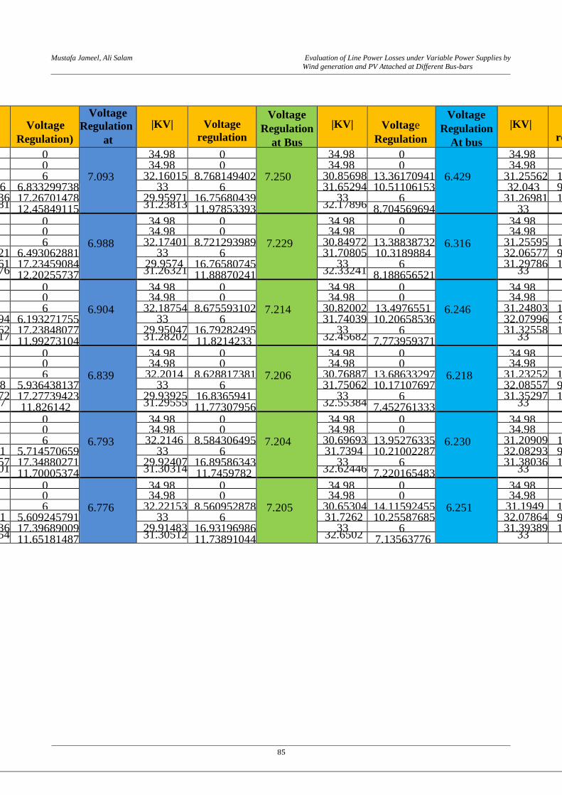
0.5MW

1 34.98 0

7.093

34.98 0

7.250

34.98 0

6.429

34.98 0

6.491

2 34.98 0 34.98 0 34.98 0 34.98 0 3 33 6 32.16015 8.768149402 30.85698 13.36170941 31.25562 11.91587305 4 32.7426 6.833299738 33 6 31.65294 10.51106153 32.043 9.165808445 5 29.82936 17.26701478 29.95971 16.75680439 33 6 31.26981 11.86508648 6 31.10481 12.45849115 31.23813 11.97853393 32.17896 8.704569694 33 6

1.5MW

1 34.98 0

6.988

34.98 0

7.229

34.98 0

6.316

34.98 0

6.461

2 34.98 0 34.98 0 34.98 0 34.98 0 3 33 6 32.17401 8.721293989 30.84972 13.38838732 31.25595 11.91469144 4 32.84721 6.493062881 33 6 31.70805 10.3189884 32.06577 9.088289475 5 29.83761 17.23459084 29.9574 16.76580745 33 6 31.29786 11.76482993 6 31.17576 12.20255737 31.26321 11.88870241 32.33241 8.188656521 33 6

2.5MW

1 34.98 0

6.904

34.98 0

7.214

34.98 0

6.246

34.98 0

6.441

2 34.98 0 34.98 0 34.98 0 34.98 0 3 33 6 32.18754 8.675593102 30.82002 13.4976551 31.24803 11.94305689 4 32.93994 6.193271755 33 6 31.74039 10.20658536 32.07996 9.04003621 5 29.83662 17.23848077 29.95047 16.79282495 33 6 31.32558 11.66592925 6 31.23417 11.99273104 31.28202 11.8214233 32.45682 7.773959371 33 6

3.5MW

1 34.98 0

6.839

34.98 0

7.206

34.98 0

6.218

34.98 0

6.431

2 34.98 0 34.98 0 34.98 0 34.98 0 3 33 6 32.2014 8.628817381 30.76887 13.68633297 31.23252 11.99864756 4 33.0198 5.936438137 33 6 31.75062 10.17107697 32.08557 9.020971109 5 29.82672 17.27739423 29.93925 16.8365941 33 6 31.35297 11.56837773 6 31.2807 11.826142 31.29555 11.77307956 32.55384 7.452761333 33 6

4.5MW

1 34.98 0

6.793

34.98 0

7.204

34.98 0

6.230

34.98 0

6.430

2 34.98 0 34.98 0 34.98 0 34.98 0 3 33 6 32.2146 8.584306495 30.69693 13.95276335 31.20909 12.08272974 4 33.0891 5.714570659 33 6 31.7394 10.21002287 32.08293 9.029942091 5 29.80857 17.34880271 29.92407 16.89586343 33 6 31.38036 11.47099651 6 31.31601 11.70005374 31.30314 11.7459782 32.62446 7.220165483 33 6

5MW

1 34.98 0

6.776

34.98 0

7.205

34.98 0

6.251

34.98 0

6.433

2 34.98 0 34.98 0 34.98 0 34.98 0 3 33 6 32.22153 8.560952878 30.65304 14.11592455 31.1949 12.13371416 4 33.1221 5.609245791 33 6 31.7262 10.25587685 32.07864 9.044523085 5 29.79636 17.39689009 29.91483 16.93196986 33 6 31.39389 11.42295523 6 31.32954 11.65181487 31.30512 11.73891044 32.6502 7.13563776 33 6



86

ble.6 (0.5-5) MW PV Generator applied at each bus and corresponding voltage regulation

Table 7 Total losses of the system and the voltage limits when extra 0.5 MW PV generators added to different buses of the system at the same time

Extra 0.5

PV generator applied

at different buses

simultaneously

Bus

Number

Voltage

(KV)

Phase

Angle

(rad)

Total System losses

Real power

(MVA)

Reactive power

(MVA)

0.5 MW PV generator

at bus 3, 4, 5, and 6

Bus 1 34.98 0

0.7345

2.1695

Bus 2 34.98 0.04524

Bus 3 33 -0.16991

Bus 4 33 -0.12495

Bus 5 33 -0.14815

Bus 6 33 -0.16008

Bus No. Voltage

KV

Active

loss

MVA

Reactive

loss

MVA

1 34.98

0.7581

2.4342

2 34.98

3 31.25298

4 32.07369

5 31.31172

6 33

Table.8 2 MW PV generator at bus 6

ISSN:2664-5564 (print) Vol 11.2( April 2021) ...

Documents

Transcript of ISSN:2664-5564 (print) Vol 11.2( April 2021) ...