ISSN: 0975-766X CODEN: IJPTFI Available Online … · Economic data are influenced by ... based on...

Shaik Khaleel Ahamed* et.al. International Journal Of Pharmacy & Technology

IJPT| June-2016 | Vol. 8 | Issue No.2 | 14666-14678 4666

ISSN: 0975-766X

CODEN: IJPTFI

Available Online through Research Article

www.ijptonline.com DATA MINING –ROBUST NEURAL REGRESSION

Shaik Khaleel Ahamed*1, C. Subba Rami Reddy

2

1PhD Scholar, C.S.E. Dept, S.V.U.College of Engineering, S.V. University, Tirupati, A.P, 517501, India.

2Professor, Statistics.Dept, S.V. University, Tirupati, A.P, 517501, India.

Emails:[email protected]

Received on 05-06-2016 Accepted on 27-06-2016

Abstract:

Robust Neural regression dealt in this article refers to a special class of inputs and outputs that are related

monotonically. The methodology is applicable to all profit and non-profit organizations whose activities can be

grouped into inputs and outputs. The samples, whose number is 145, belong to the inputs and output of Indian

Commercial Banks. The outliers/influential observations are identified using efficient and inefficient Data

Envelopment Analysis. DEA is a linear programming technique. Neural linear and non-linear regressions are fitted to

examine the presence of specification error that we come across in statistical Multiple Linear Regression. The

empirical results reveal mild presence of specification error if linear regression is preferred to non-linear regression.

Keywords: Robust Neural Regression, outliers/influential observations, Data Envelopment Analysis.

1. Introduction:

The property of ‘monotonicity’ between inputs and outputs has an important role to play in profit and non-profit

organizations in which similar inputs are combined to produce similar outputs. In production economics, production

functions represent technological relationships that are assumed to satisfy monotonicity between inputs and outputs.

If x produces y and 'x produces

'y and if 'x x then

'y y .

To fit a parametric production frontier one needs production plans such that each production plan neither dominates

nor dominated by other production plans. But, the firms comprising an industry employ different techniques and

several of them are found to be dominated by a small number of firms. If such empirical data are confronted with a

parametric frontier the statistical estimates often contradict the theoretical postulates such as the property of

monotonicity. The effective alternative to a parametric production function is the non-parametric production function

introduced by Charnes, Cooper and Rhodes (CCR, 1978)1, subsequently generalized by Banker, Charnes and Cooper

(BCC, 1984)2. The particulars of their production frontiers are embedded in linear programming constraints and their

mailto:[email protected]


IJPT| June-2016 | Vol. 8 | Issue No.2 | 14666-14678 Page 14667

structure cannot be visualized as otherwise in the case of parametric frontiers. The CCR production frontier is the

surface of the Production Possibility Set based on the postulates, inclusion, ray unboundedness, free disposability and

minimum extrapolation. Economic data are influenced by returns to scale, constant or increasing or decreasing. The

most ideal version of returns to scale are constant and the CCR frontier admits the same. But, the BCC frontier

accomodates all the three types of returns to scale, whose Production Possibility Set is built on the axioms, inclusion,

convexity, free disposability and minimum extrapolation. The very widely used production functions in production

economics are multiple linear regression equivalents, which can be fitted by the method of least squares.

2. Outliers:

There are several sources which would result in bad multiple linear regression estimates. An important source of

distorted regression results is the presence of outliers which deviate radically from normal observations. In statistical

linear regression estimation, leverages, JackKnife residuals, Studentised residuals and Cook’s Distance3 are employed

to detect outliers. These methods are parametric based.

Data Envelopment Analysis (DEA) proposed by CCR (1978) and generalized by BCC (1984) is a linear

programming based technique that estimates technical efficiency of decision making units (DMUs). DEA efficiency

scores are sensitive to outliers. In order to find robust efficiency scores, the outliers are to be identified and removed.

Andersen and Petersen (1993)3 introduced the concept of super efficiency of extremely efficient decision making

units. Such extremely efficient production plan whose deletion from the reference set contracts the Production

Possibility Set the most is the most influential observation.

Wilson (1995)4 proposed a method based on leave-one-out approach and the search was for outliers among the

extremely efficient production units. Stocic and Sampario de Souza (2003, 2005)5, 6

proposed an outlier detection

method based on a combination of bootstrap and resampling schemes. Trans et.al (2008)7 initiated a methodology

based on peer count and sum of intensity parameters for the identification of DEA outliers/most influential

observations.

Chen and Johnson (2010)8 considered Convex Hull as the Production Possibility Set and provided a leverage based

methodology to identify outliers. Ahmed et.al (2015, 2015, 2016)9, 10, 11

proposed a new method to identify outliers

from among the extremely efficient and extremely inefficient production plans. It is a leave-one-out approach. To

identify efficient outliers efficient frontier and inefficient outliers inefficient frontier based linear programming

problems are to be solved. The present study uses the new method to identify efficient and inefficient suspected

outliers.



3. Artificial Neural Network (ANN) Regression:

Robust regression in this study refers to a special class where inputs are monotone with outputs. Solving the CCR

linear programming problems input technical efficiencies can be estimated for decision making units. The input and

output plans can be arranged in ascending order of technical efficiency scores. Such production units whose input and

output plans are closer to the production frontier (high efficiency scores) satisfy the monotonicity property with

greater probability than those distant from the DEA frontier.

An alternative to statistical multiple linear regression is artificial neural network (ANN) based linear and non-linear

regression. Artificial neural networks are mathematical models mimic the function of human brain trained by

optimization algorithms, while training may be Supervised or Unsupervised. ANN does not explicitly specify the

functional form that is assumed to have generated the samples.

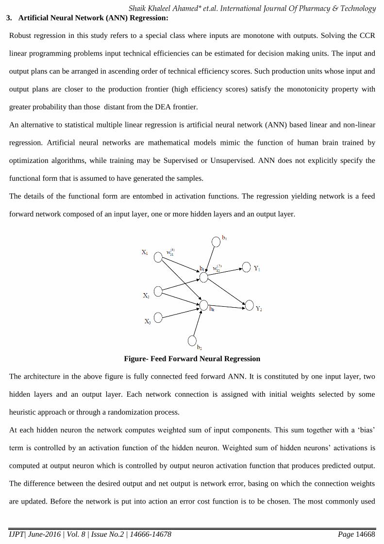
The details of the functional form are entombed in activation functions. The regression yielding network is a feed

forward network composed of an input layer, one or more hidden layers and an output layer.

Figure- Feed Forward Neural Regression

The architecture in the above figure is fully connected feed forward ANN. It is constituted by one input layer, two

hidden layers and an output layer. Each network connection is assigned with initial weights selected by some

heuristic approach or through a randomization process.

At each hidden neuron the network computes weighted sum of input components. This sum together with a ‘bias’

term is controlled by an activation function of the hidden neuron. Weighted sum of hidden neurons’ activations is

computed at output neuron which is controlled by output neuron activation function that produces predicted output.

The difference between the desired output and net output is network error, basing on which the connection weights

are updated. Before the network is put into action an error cost function is to be chosen. The most commonly used



error function is the mean square error, and the same is used in the present study. An alternative to mean square error

is cross entropy, which requires data transformation before it is kept in use. The feed forward networks are trained by

Back Propagation whose algorithm is supported by an optimization technique. In this study the algorithms are

supported by the Conjugate Descent12

, Levenberg-Marquardt13

and Resilient Propagation Method14

.

Activation functions control signals of hidden and output layers. The activation functions implemented in this study

are linear that provides neural linear regression and tangent sigmoid that gives neural non-linear regression.

In ANN it is customary to divide the samples into three sets each serving a different purpose, the purposes being

training, validation and testing. The samples of training set are fed into the network through input layer, which allow

the network to learn the structure of the data. If a network is trained hard it may learn noise leading to over fitting.

Consequently the learned model performs poorly while it is tested. To locate the training point beyond which the

network may over learn, the validation set is used. Weights are not updated on the validation set. If network’s

performance is improved during training, the same is felt in validation. Eventually, a point is reached beyond which

the training error diminishes, but the validation error either remains to be the same or kept increasing. This is the

point at which over fitting commences which signals training to be stopped. The testing set reveals the predictive

capability of the trained neural net. In this study the observations are split such that 70, 15 and 15 percent of the total

number of samples constitute training, validation and testing set respectively.

4. Neural Regression:

Statistical Multiple Linear Regression (MLR) suffers from model specification error. In a single explanatory variable

context consider the following non-linear relationship that is thought to have generated the samples:

( )y f x

From Tailor’s series expansion around 0x , we have,

' 2' ''(0) (0) (0) ....

1 2

x xy f f f

y a bx

where (0)a f

' (0)b f

is the specification error.



The neural non-linear regression is free from specification error, provided that the network, error function and the

activation function are cautiously selected. The ANN regression is non-parametric like DEA, where as its counterpart

statistical MLR is parametric. In ANN regression dimensional increase requires exponential increase in sample size,

while the relationship between number of dimensions and sample size is linear in statistical MLR. In neural

regression the modler shall exercise caution while explanatory variables are chosen, since neural regression cannot

reject an irrelevant variable which is otherwise in statistical regression. Individual explanatory variable impact on the

dependent variable cannot be measured in ANN regression, in sign and magnitude. 2 2( )R or adjusted R is the only

performance indicator of neural regression. No statistical significance tests prevail on neural regression. A neural net

trained by sufficiently large number of samples possesses adequate testing power.

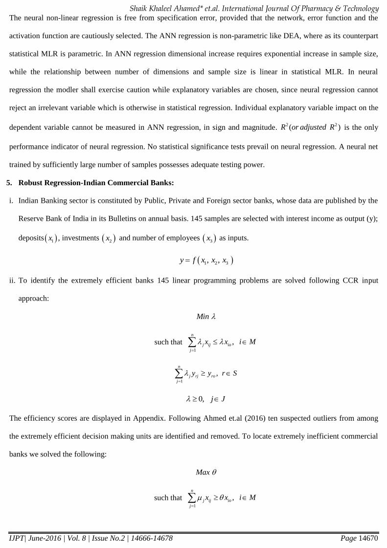
5. Robust Regression-Indian Commercial Banks:

i. Indian Banking sector is constituted by Public, Private and Foreign sector banks, whose data are published by the

Reserve Bank of India in its Bulletins on annual basis. 145 samples are selected with interest income as output (y);

deposits 1x , investments 2x and number of employees 3x as inputs.

1 2 3, ,y f x x x

ii. To identify the extremely efficient banks 145 linear programming problems are solved following CCR input

approach:

Min

such that 1

, n

j ij io

j

x x i M

1

,n

j rj ro

j

y y r S

0, j J

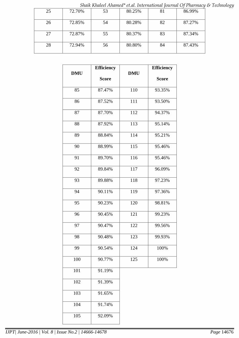
The efficiency scores are displayed in Appendix. Following Ahmed et.al (2016) ten suspected outliers from among

the extremely efficient decision making units are identified and removed. To locate extremely inefficient commercial

banks we solved the following:

Max

such that 1

, n

j ij io

j

x x i M



1

, n

j rj ro

j

y y r S

0, j J

Nine suspected outliers from extremely inefficient production plans were identified and removed. Consequently, we

are left with 125 samples.

iii. The samples are arranged in ascending order of their input technical efficiency scores, then divided into 3 sets, low

efficient layer 1L , medium efficient layer 2L and high efficient layer 3L .The 1L layer consists of the

inputs and outputs of the first 45 commercial banks that are low efficient. The 2L layer contains the input and

of output plans of 35 medium efficient banks. The activities of high efficient group of 45 commercial banks

belong to layer 3L .

iv. Log linear production functions were very widely and successfully used in empirical studies of production

economics. Two such frontier production functions are,

a) Cobb-Douglas production function15

and

b) Transcendental logarithmic production function16

. Keeping this in mind inputs and output are pre-

processed by taking logarithms. For faster convergence of ANN algorithms all variable values are suitably

scaled to fall between zero and one.

v. The low efficient production plans 1L that are well below the frontier may fail to satisfy the monotonicity

property. If network is trained with these 45 samples, the network may not learn monotonicity adequately. Further,

the predictions provide poor targets for banks of layer 1L . The production plans of 2L which satisfy the

monotonicity property fairly were augmented to 1L so that we have 1 2L L (80 samples). Further 1 2L L

provides more observations for training than 1L alone.

vi. The high efficient production plans 3L very fairly satisfy the property of monotonicity as these either fall on the

frontier, if not, distributed very close to frontier. If the samples of 3L are presented to the ANN, it learns

monotonicity property very well, but fail to learn normal samples. Therefore, 2L is augmented to 3L . 2 3L L

provides 80 samples for training, validation and testing.

vii. Finally, all three layers we combined 1 2 3( )L L L and all the 125 observations are fed into the net for training,

validation and testing.



viii. Before the samples were fed into the net, they were randomized. 70-15-15 percent of the samples were

allocated for training, validation and testing respectively.

6. Empirical Performance Of Ann Regression:

The difficulties associated with ANN involve choosing the network’s parameters such as the number of hidden layers

and neurons in each layer, the initial weights, and the step size of learning. The process of determining appropriate

values of these is often an experimental issue and time consuming. On trial and error basis we found 7 neurons feed

forward ANN is appropriate for neural regression estimation. The neural regression results are as follows:

a. (i) Neural Linear Regression-Low efficient and Medium efficient combined 1 2L L :

The activation function administered on ANN is linear and Training Algorithms are based on Gradient Descent,

Levenberg-Marquardt and Resilient Propagation optimization method. 1 2 3

ˆˆ ( , , )y f x x x

SNO OPTIMIZATION

PRINCIPLE

TRAIN R TEST R ALL R MSE

1 LM 0.9867 0.98755 0.9867 0.00206

2 GDM 0.9802 0.9695 0.9785 0.00319

3 RP 0.9809 0.9916 0.9838 0.00198

Table (1)

The activation function administered on the neural network is linear. The best neural linear regression is provided by

the Resilient Propagation, identified basing on its testing performance.

a. (ii) Neural Non-linear Regression for (L1+L2):

The non-linear activation function imposed is Tangent Sigmoid. LM, GDM and RP are the optimization methods

supported the Training Algorithms.

SNO OPTIMIZATION

PRINCIPLE

TRAIN

R

TEST

R

ALL

R

MSE

1 LM 0.9981 0.9868 0.9968 0.000236

2 GDM 0.9499 0.9572 0.9489 0.00669

3 RP 0.9940 0.9894 0.9917 0.00067

Table (2)

1 2 3ˆˆ ( , , )y f x x x



With tangent sigmoid as the activation function, the training algorithm based on Levenberg-Marquardt method and

Resilient Propagation produced best results for neural non-linear regression.

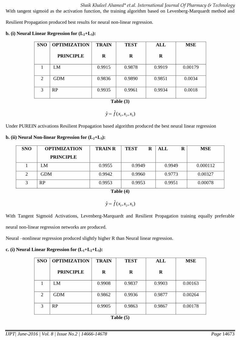
b. (i) Neural Linear Regression for (L2+L3):

SNO OPTIMIZATION

PRINCIPLE

TRAIN

R

TEST

R

ALL

R

MSE

1 LM 0.9915 0.9878 0.9919 0.00179

2 GDM 0.9836 0.9890 0.9851 0.0034

3 RP 0.9935 0.9961 0.9934 0.0018

Table (3)

1 2 3ˆˆ ( , , )y f x x x

Under PUREIN activations Resilient Propagation based algorithm produced the best neural linear regression

b. (ii) Neural Non-linear Regression for (L2+L3):

SNO OPTIMIZATION

PRINCIPLE

TRAIN R TEST R ALL R MSE

1 LM 0.9955 0.9949 0.9949 0.000112

2 GDM 0.9942 0.9960 0.9773 0.00327

3 RP 0.9953 0.9953 0.9951 0.00078

Table (4)

1 2 3ˆˆ ( , , )y f x x x

With Tangent Sigmoid Activations, Levenberg-Marquardt and Resilient Propagation training equally preferable

neural non-linear regression networks are produced.

Neural –nonlinear regression produced slightly higher R than Neural linear regression.

c. (i) Neural Linear Regression for (L1+L2+L3):

SNO OPTIMIZATION

PRINCIPLE

TRAIN

R

TEST

R

ALL

R

MSE

1 LM 0.9908 0.9837 0.9903 0.00163

2 GDM 0.9862 0.9936 0.9877 0.00264

3 RP 0.9905 0.9863 0.9867 0.00178

Table (5)



1 2 3ˆˆ ( , , )y f x x x

Imposing PUREIN activation functions on neural regression network. Levenberg-Marquardt and Resilient

Propagation principle based back propagation provides, best regression results.

c. (ii) Neural Non- Linear Regression for (L1+L2+L3):

SNO OPTIMIZATION

PRINCIPLE

TRAIN

R

TEST

R

ALL

R

MSE

1 LM 0.9971 0.9980 0.9970 0.000428

2 GDM 0.9963 0.9625 0.9370 0.0114

3 RP 0.9910 0.9893 0.9900 0.00120

Table (6)

1 2 3ˆˆ ( , , )y f x x x

Best neural non-linear regression fit is provided by LM based algorithm for Y.

7. Conclusions:

Robust neural Regression requires careful data pre-processing, in terms of elimination of outliers, selection of

relevant explanatory variables, exercising parsimony in dimensional selection, control of variation in inputs and

outputs values. It also requires judicious choice of hidden layers and number of neurons in each of such layers, size of

learning step, error function, activation functions and the optimization principle that supports the training algorithm.

The statistical multiple linear regression suffers from specification error of some degree, serious or negligible. Before

a statistical MLR is selected for estimation, it is better to know if the specification error is serious or negligible,

examining the R (or adjusted R) values of neural linear and non-linear regression. Comparing the best of neural linear

and non-linear regressions we find that specification error is of negligible magnitude, implying the appropriateness of

multiple linear regression in statistical estimation. Neural regression fails to identify irrelevant variables that enter

due to the ignorance of the researcher. Entry of irrelevant variables require samples number to increase at exponential

rate, disturbs model training forcing the training error trapped in local minima. Before neural regression is

implemented, it is appropriate to identify irrelevant variables using adjusted R2 of statistical MLR.

Neural regression fits cannot explicitly reveal if the property of monotonicity17

is really satisfied by the model, since

the model details are buried in the activation functions. The differential impacts of explanatory variables on the

dependent variables cannot be measured in neural regression.



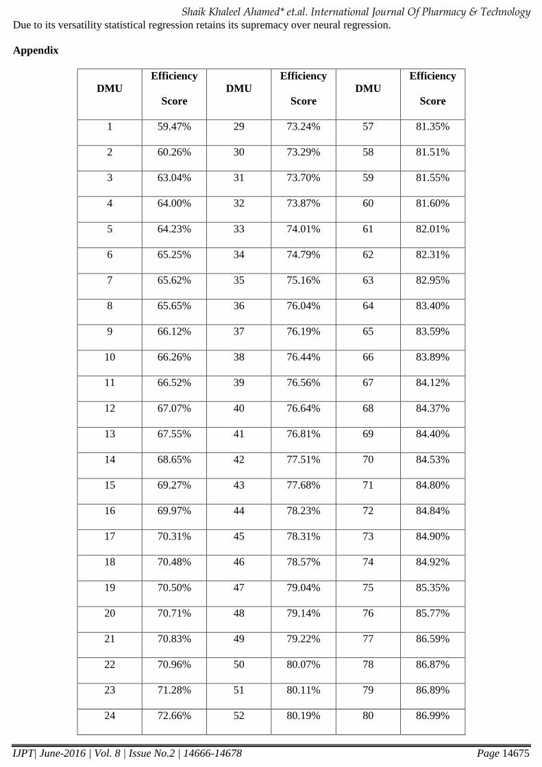
Due to its versatility statistical regression retains its supremacy over neural regression.

Appendix

DMU

Efficiency

Score

DMU

Efficiency

Score

DMU

Efficiency

Score

1 59.47% 29 73.24% 57 81.35%

2 60.26% 30 73.29% 58 81.51%

3 63.04% 31 73.70% 59 81.55%

4 64.00% 32 73.87% 60 81.60%

5 64.23% 33 74.01% 61 82.01%

6 65.25% 34 74.79% 62 82.31%

7 65.62% 35 75.16% 63 82.95%

8 65.65% 36 76.04% 64 83.40%

9 66.12% 37 76.19% 65 83.59%

10 66.26% 38 76.44% 66 83.89%

11 66.52% 39 76.56% 67 84.12%

12 67.07% 40 76.64% 68 84.37%

13 67.55% 41 76.81% 69 84.40%

14 68.65% 42 77.51% 70 84.53%

15 69.27% 43 77.68% 71 84.80%

16 69.97% 44 78.23% 72 84.84%

17 70.31% 45 78.31% 73 84.90%

18 70.48% 46 78.57% 74 84.92%

19 70.50% 47 79.04% 75 85.35%

20 70.71% 48 79.14% 76 85.77%

21 70.83% 49 79.22% 77 86.59%

22 70.96% 50 80.07% 78 86.87%

23 71.28% 51 80.11% 79 86.89%

24 72.66% 52 80.19% 80 86.99%



25 72.70% 53 80.25% 81 86.99%

26 72.85% 54 80.28% 82 87.27%

27 72.87% 55 80.37% 83 87.34%

28 72.94% 56 80.80% 84 87.43%

DMU

Efficiency

Score

DMU

Efficiency

Score

85 87.47% 110 93.35%

86 87.52% 111 93.50%

87 87.70% 112 94.37%

88 87.92% 113 95.14%

89 88.84% 114 95.21%

90 88.99% 115 95.46%

91 89.70% 116 95.46%

92 89.84% 117 96.09%

93 89.88% 118 97.23%

94 90.11% 119 97.36%

95 90.23% 120 98.81%

96 90.45% 121 99.23%

97 90.47% 122 99.56%

98 90.48% 123 99.93%

99 90.54% 124 100%

100 90.77% 125 100%

101 91.19%

102 91.39%

103 91.65%

104 91.74%

105 92.09%



106 92.65%

107 92.68%

108 92.87%

109 92.90%

References:

1. Charnes, A., Cooper, W.W., Rhodes, E, ‘Measuring the efficiency of Decision Making Units’. European Journal

of Operational Research, (1978); 2: 429-444.

2. Banker, R. D., Charnes, R.F, Cooper, W.W, ‘Estimating Most Productive Scale Size Using Data Envelopment

Analysis’. European Journal of Operations Research, (1984); 30: 35-44.

3. Andersen, P., Petersen, N.C, ‘A Procedure for Ranking Efficient Units in Data Envelopment Analysis’,

Management Science, (1993); 39:1261-1264.

4. Wilson, P.W., ‘Detecting Influential Observations in Data Envelopment Analysis’, Journal of Productivity

Analysis, (1995); 4: 27–45.

5. Stosic, B., Sampaio de Sousa, M. C., ‘Jackstrapping DEA Scores for Robust Efficiency Measurement.’ Anais do,

Encontro Brasileiro de Econometria SBE,25; (2003): 1525-1540.

6. Sampaio de Sousa, M. C. and Stosic, B. ‘Technical Efficiency of the Brazilian Municipalities: Correcting

Nonparametric Frontier Measurements for Outliers.’ Journal of Productivity Analysis, (2005); 24: 157-181.

7. Tran, N.A., Sheverly, G., Preckel, P., ‘A New Method for detecting Outliers in DEA’, Applied Economic

Letters, (2008); 15(1): 1-4.

8. Chen, Johnson, ‘A Unified model for detecting Outliers in DEA’, Computers and Operations Research, (2010);

37 :417-425.

9. Ahamed, S.K., Naidu, M.M., Subba Rami Reddy, C, ‘Outliers in Data Envelopment Analysis’, International

Journal of Computer Science and Security (IJCSS), (2015); 9(3): 164-173.

10. Ahamed, S.K., Naidu, M.M., Subba Rami Reddy, C, ‘Most Influential Observations Super Efficiency’,

International Journal on Computer Science and Engineering (IJCSE), (2015); 7(9): 82-96.

11. Ahamed, S.K., Naidu, M.M., Subba Rami Reddy, C, ‘Outliers/Most Influential Observations in Variable Returns

to Scale Data Envelopment Analysis’, Indian Journal of Science and Technology, (2016); 9(2): 1-7.

12. Cobb, C. W., Douglas, P. H. ‘A Theory of Production’. American Economic Review, (1928); 18: 139–165.

https://en.wikipedia.org/wiki/American_Economic_Review



13. Hestenes, Magnus R.; Stiefel, Eduard, "Methods of Conjugate Gradients for Solving Linear Systems" (PDF).

Journal of Research of the National Bureau of Standards,(1952); 49 (6).

14. Kenneth Levenberg, ‘A Method for the Solution of Certain Non-Linear Problems in Least Squares’, Quarterly

Journal of Applied Mathematics, (1944); 2: 164–168.

15. Martin Riedmiller und Heinrich Braun: Rprop – ‘A Fast Adaptive Learning Algorithm’, Proceedings of the

International Symposium on Computer and Information Science VII, (1992).

16. Christensen, L.R., Jorgenson, D.W., Lau, J, ‘Transcendental Logarithmic Production Frontiers’, The Review of

Economics and Statistics, (1973); 55: 28-45.

17. P.C. Pendharkar, “A Data Envelopment Analysis-Based Approach for Data Preprocessing,” IEEE Transactions

on Knowledge & Data Engineering, (2005); 17(10):1379-1388.

Corresponding Author:

Shaik Khaleel Ahamed*,

Emails: [email protected]

https://en.wikipedia.org/wiki/Magnus_Hestenes

https://en.wikipedia.org/wiki/Magnus_Hestenes

https://en.wikipedia.org/wiki/Eduard_Stiefel

http://nvl.nist.gov/pub/nistpubs/jres/049/6/V49.N06.A08.pdf

mailto:[email protected]

ISSN: 0975-766X CODEN: IJPTFI Available Online … · Economic data are influenced by ... based on...

Documents

Transcript of ISSN: 0975-766X CODEN: IJPTFI Available Online … · Economic data are influenced by ... based on...