ISPD’2005 Fast IntervalValued Statistical Interconnect Modeling And Reduction

ISPD’2005

Fast Interval Valued StatisticalInterconnect Modeling And Reduction

ISPD’2005

Fast Interval Valued StatisticalInterconnect Modeling And Reduction

James D. Ma and Rob A. Rutenbar

Dept of ECE, Carnegie Mellon University {jdma, [email protected]}

Funded in part by C2S2, the MARCO Focus Center for Circuit & System Solutions

New Battlefield: Manufacturing Variations

CMOS scaling… Good for speed Good for density

BOXBOX

BOX

Bad for variation Bad for manufacturability Bad for predictability

No longer realistic to regard device or interconnect as deterministic

Continuous random distribution with complex correlations

New Problem: Statistical Analysis

Statistical static timing analysis Propagate correlated

normal distribution A limited number of

operators: sum and maximum

Statistical interconnect timing analysis Require a richer palette

of computations Not easy to represent

statistics and push them through model reduction algorithms

?

?

max,

max,

Approaches to Statistical Interconnect Analysis

Straight-forward Monte Carlo simulation Repeat model reduction algorithms at the outermost loop General, accurate, but computationally expensive

Control-theoretic (model order reduction) Based on perturbation theory [Liu-et al, DAC’99] Multi-parameter moment matching [Daniel-et al, TCAD’04]

Circuit performance evaluation Low-order analytical delay formula [Agarwal-et al, DAC’04] Asymptotic non-normal probability extraction [Li-et al, ICCAD’04] Classical interval delay analysis [Harkness-Lopresti, TCAD’92]

Our interest — new correlated interval technique for representing statistics “inside” algorithms

New Interval Ideas

Classical interval Define two end-points No “inside” information Unable to consider

correlations

Affine interval Define central point and radius Keep source of uncertainties Handles correlations by

uncertainty sharing

hilo

2-2

1-1 1-1

x

x – x

x = x0 + x1 1 + x2 2

R (xa) = | x1 | + | x2 |

x0-x1 x1 x2-x2

x – x = (x0 – x0) +

(x1 – x1) 1 + (x2 – x2) 2

= 0

Should be 0 !

Affine Arithmetic: An Overview

Develop a library for most affine arithmetic operations More accurate or efficient approximations are also available

x = x0 + ∑ xi i

y = y0 + ∑ yi i

z = x0 + y0 + ∑ (xi + yi) iz = x0 y0 + ∑(x0 yi + y0 xi) εi

+ (∑xi εi) (∑xi εi)

z = x0 y0 + ∑(x0 yi + y0 xi) εi + R (xy) ζ

Results are still affine (accurate or conservative)

Replace second-order terms withone new uncertainty term ζ

From Intervals to Statistics

Statistical assumption for the uncertainty symbols?

Choose normal distribution μ = 0, σ2 = 1 for each symbol εi

Probability not equal in the interval Model the central mass of the

infinite, continuous distribution

Uniform distribution? Keep conservative bounds Not realistic for modeling

manufacturing variations

Essential assumption Mechanics of calculation for finite affine intervals are a reasonably good

approximation of how statistics move through the same computations

Putting Altogether: From Intervals to Algorithms

Scalar-valued linear solve Backward substitution

Classical interval-valued linear solve Backward substitution Classical interval arithmetic

=[1 5] 0 [1 7]0 [1 3] [1 5]0 0 [–6 –2]

x1

x2

x3

–1–10 16

= [0.3 55][–7.3 30][–8 –2.7]

x1

x2

x3

3 0 40 2 30 0 –4

x1

x2

x3

= –1–10 16

x1

x2

x3

= 5 1–4

From Intervals to Algorithms (Cont’d)

Affine interval-valued linear solve

Sample matrix element intervals& scalar solve

Polytope for the range of x1, x2, x3A

ffine

Cube for the range of x1, x2, x3

Cla

ssic

al

=3 + ε1 + ε2 0 4 – ε1 + 2ε3

0 2 + ε1 3 + ε1 – ε3

0 0 –4 + ε1 – ε3

x1

x2

x3

–1–10 16

=x1

x2

x3

5 – 3ε1 – 3 ε2 + 1.8ε3 – 2.7ε5 1 + 3.4ε1 – 4ε3 – 2.3ε4

–4 – ε1 + ε3

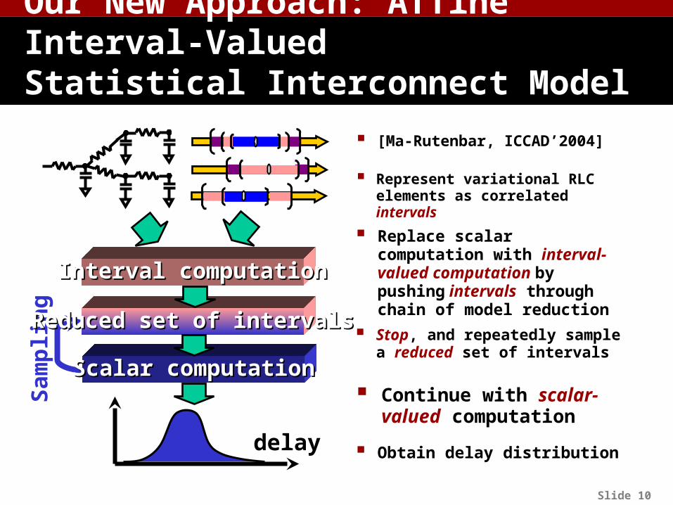
Our New Approach: Affine Interval-Valued Statistical Interconnect Model Reduction

Represent variational RLC elements as correlated intervals

Interval computationInterval computation

Sam

plin

g Reduced set of intervalsReduced set of intervals

Scalar computationScalar computation

delay

Replace scalar computation with interval-valued computation by pushing intervals through chain of model reduction

Stop, and repeatedly sample a reduced set of intervals

Continue with scalar-valued computation

Obtain delay distribution

[Ma-Rutenbar, ICCAD’2004]

Interval Modeling of Interconnect Parameters

Global variations — inter-die Affect all the device and interconnect, in a similar way

Local variations — intra-die Affect device and interconnect close to each other, in a similar way

Linearized combination of global and local variations

One variation source may contribute to multiple RLC’s & lead to correlation

Any variation can have positive or negative impact on RLC

R = R0 + ∑(∆Ri i ) + ∑(∆Rj j) + ∑(∆Rk k)

C = C0 + ∑(∆Ci i ) + ∑(∆Cj j) – ∑(∆Ck k)

L = L0 + ∑(∆Li i ) – ∑(∆Lj j) – ∑(∆Lk k)Affi

ne fo

rms

Interval-Valued AWE: 1st Generation

Interval-valued MNA and LU for model reduction

Interval-valued pole/residue analysis

Mostly fundamental affine operations

Compare intervals based on their central values

Obtain a reduced, small set of interval poles and residues

Sample and continue scalar transient analysis

Monte Carlo sampling over this reduced model is very fast

Similar approach for interval-valued PRIMA

LU decompositionLU decomposition

Solve for residuesSolve for residues

Delay distributionDelay distribution

Solve for polesSolve for poles

MNA formulationMNA formulation

Sam

plin

g Poles/residuesPoles/residues

Transient analysisTransient analysis

Hankel matrix & vectorHankel matrix & vector

Vandemonde matrixVandemonde matrixIn

terv

als

Inte

rval

sSc

alar

sSc

alar

s

Interval-Valued AWE: 2nd Generation

1st improvement Replace MNA formulation & LU decomposition with path-tracing for

tree-structured circuits to compute interval-valued moments much more efficiently

1 2

3 4

5 6

0

0 1 2 3

5

4

6

C

C

C

C

R

R

R

R

R

2nd improvement Stop interval-valued computation at moments, not poles/residues Then switch to sampling and scalar-valued computation

1st Improvement: Interval LU vs. Path-Tracing

Interval estimation errors Like floating-point errors, but more macroscopic, not so easy to ignore The longer the chain of computation, the more errors

LU decomposition

rang

e

Replace interval LU with interval path-tracing Reduce number of approximate affine operations significantly Improve greatly both efficiency and accuracy

Path-tracing

rang

e

Path-tracing — DC analyses for moments via depth-first search Tree topology does not change — DFS only once Tracing order can be stored and “remembered”

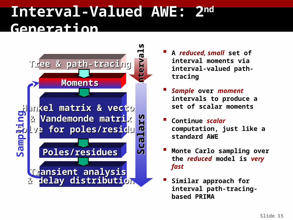
Interval-Valued AWE: 2nd Generation

A reduced, small set of interval moments via interval-valued path-tracing

Sample over moment intervals to produce a set of scalar moments

Continue scalar computation, just like a standard AWE

Monte Carlo sampling over the reduced model is very fast

Similar approach for interval path-tracing-based PRIMA

Inte

rval

sIn

terv

als

MomentsMoments

Hankel matrix & vectorHankel matrix & vector& Vandemonde matrix& Vandemonde matrix

Solve for poles/residuesSolve for poles/residues

Sam

plin

g

Poles/residuesPoles/residues

Transient analysis Transient analysis & delay distribution& delay distribution

Tree & path-tracingTree & path-tracing

Scal

ars

Scal

ars

2nd Improvement: AWE Interval/Scalar Tradeoff

Interval MNA & LUInterval MNA & LU

Interval momentsInterval moments

Interval root findingInterval root finding

Interval poles/residuesInterval poles/residues

Scalar delayScalar delaySam

plin

g

Inte

rval

sIn

terv

als

Scal

ars

Scal

ars

Inte

rval

sIn

terv

als

Scal

ars

Scal

ars

Interval tree Interval tree & path-tracing& path-tracing

Interval momentsInterval moments

Scalar root findingScalar root finding

Scalar poles/residuesScalar poles/residues

Scalar delayScalar delay

Sam

plin

g

1st generation Pervasive interval computation

2nd generation Hybrid interval/scalar strategy

Interval computation for large-scale near-linear model reduction Scalar sampling & small-scale nonlinear root finding Similar tradeoff for 2nd generation of interval-valued PRIMA

Benchmarks

ε1

ε2

ε3

ε4

ε5

3 tree-structured RC(L) interconnects From 120 to 2400 elements Deterministic unit step input

6 — 21 variation symbols One global, shared by all RLC’s Others local, shared by a

cluster of “nearby” RLC’s

Relative σ of global / local vars 20% / 10%, 10% / 20%, 5% / 30%

Able to accommodate Any number of uncertainties, from most types of variation sources Any reasonable combinations of global / local variations

2nd Generation: Implementation

Interval arithmetic library and AWE/PRIMA in C/C++ Compare distribution of 50% delay

2nd generation (statAWE/statPRIMA) vs. RICE 4/5 used in a simple Monte Carlo loop (RMC)

Determine proper number of Monte Carlo samples using standard confidence interval techniques [Burch-et al, TVLSI’93]

Specify accuracy within 1%, with 99% confidence level ~ 3000 samples for each design combination

Sample RC(L)’s Sample RC(L)’s

ScalarScalar AWE/PRIMA AWE/PRIMAMon

te C

arlo

RC(L) intervalsRC(L) intervalsIntervalInterval AWE/PRIMA AWE/PRIMA

Sample intervalsSample intervals

Mon

te C

arlo

vs.

Monte Carlo simulation

10000 samples of RLC’s

Pole Distribution

At the end of 2nd generation interval AWE/PRIMA, an interval-valued reduced model is obtained

How well do the reduced interval model produce scalar poles?

design0, 123 RLC’s, 5% global variation, 30% local variation, 6 variation terms, 8th order AWE, distributions of 4 dominant poles on complex plane

Interval-valued estimation

10000 samples in moment intervals

Interval

Monte Carlo

0%

5%

10%

15%

20%

delay

25%

Accuracy & Efficiency

Mean Delay Err Stdev Err Speed-upstatAWE1.7% 1.8% 11

statPRIMA2.5% 2.6% 10

AWE

0%

5%

10%

15%

20%

25%

delay

Interval

Monte Carlo

PRIMA

Delay PDFs ex: 1275 RC’s, 5% global, 30% local, 4th order models

CPU time: 1 interval analysis ≈ 300 deterministic runs

Interval/Scalar Tradeoff

Interval Path-tracing MNA & LU

Moments I (2nd gen.) II

Poles/residues III IV (1st gen.)

Compare 4 AWE interval strategies

0

0.5

1

1.5

2

2.5

3

3.5

0% 2% 4% 6% 8% 10%mean error

log

(ru

n t

ime

)

IIV

II

III

Run time vs. mean error

0

0.5

1

1.5

2

2.5

3

3.5

0% 2% 4% 6% 8%std error

log

(ru

n t

ime

)

III

IVII

I

Run time vs. std error

If ~5–10% error is OK, one can still use intervals pervasively 1st 2nd generation: ~10X less CPU, ~3–4X less %error

Conclusions and Ongoing Work

Affine interval model & statistical interpretation allow us to Represent the essential mass of a random distribution Preserve 1st-order correlations among uncertainties Retarget classical model reduction to interval-valued computations

Improved 2nd generation Smarter interval linear solves and interval/scalar tradeoffs ~10X faster, and ~3–4X less %error

What’s next? Works well for interconnect reduction – but how general is the idea? Can we bring statistics into arbitrary CAD tools efficiently? In progress: interval-valued physics-based TCAD/DFM modeling

ISPD’2005 Fast IntervalValued Statistical Interconnect Modeling And Reduction

Documents

Transcript of ISPD’2005 Fast IntervalValued Statistical Interconnect Modeling And Reduction