Isolated Word Speech Recognitionpfelber/speechrecognition/report.pdf · SPEECH RECOGNITION Report...
76
SPEECH RECOGNITION Report of an Isolated Word experiment. By Philip Felber Illinois Institute of Technology April 25, 2001 Prepared for Dr. Henry Stark ECE 566 Statistical Pattern Recognition
Transcript of Isolated Word Speech Recognitionpfelber/speechrecognition/report.pdf · SPEECH RECOGNITION Report...

SPEECH RECOGNITION
Report of an Isolated Word experiment.
By Philip Felber
Illinois Institute of Technology
April 25, 2001
Prepared for Dr. Henry Stark
ECE 566 Statistical Pattern Recognition
4/25/2001 ECE566 Philip Felber 2
ABSTRACT
Speech recognition is the analysis side of the subject of machine speech
processing. The synthesis side might be called speech production. These two
taken together allow computers to work with spoken language. My study
concentrates on isolated word speech recognition. Speech recognition, in
humans, is thousands of years old. On our planet it could be traced backed
millions of years to the dinosaurs. Our topic might better be called automatic
speech recognition (ASR). I give a brief survey of ASR, starting with modern
phonetics, and continuing through the current state of Large-Vocabulary
Continuous Speech Recognition (LVCSR). A simple computer experiment,
using MATLAB, into isolated word speech recognition is described in some
detail. I experimented with several different recognition algorithms and I used
training and testing data from two distinct vocabularies. My training and
testing data was collected and recorded with both male and female voices.
4/25/2001 ECE566 Philip Felber 3
BUZZWORDS - OK WORDS
Cepstrum. Coefficients of the Fourier transform representation of the log magnitude of the spectrum; Normally derived from the LPC coefficients. Cepstral analysis provides a method for separating the vocal tract information from the vocal cord excitation.
Formants. Spectral peaks in the sound of a voice. For voiced phonemes, the sound spectrum involves frequency bands with large concentrations of energy called formants.
Linear Predictive Coding (Coefficients). Speech can be modeled as if it were produced by an IIR filter, driven by a pulse source (voiced utterance) or white noise (unvoiced utterance). The LPC coefficients describe such a filter in that they are the best (in a least squares sense) fit over a short time interval.
Phonemes and phones (allophones). Phonemes are the smallest parts of spoken words. A set of phonemes can be defined as the minimum number of symbols needed to describe every possible word in a language. Phonemes are abstract units, and during speech there actual pronunciation varies. These variations are called phones or, more correctly, allophones.
Phons and sones. Human hearing sensitivity varies with frequency. If a given sound is perceived to be as loud as a 60 dB 1000 Hz sound, then it is said to have a loudness of 60 phons. Phons track (at least for a given frequency) with dBs. Sones are spaced as a linear scale. One sone being equivalent to 40 phons (dBs), and doubling for each 10 phons thereafter. 100 phons is then equivalent to 64 sones.
Pre-emphasis filter. Sloped filter used to compensate for the higher energy of the lower (frequency) formants.

4/25/2001 ECE566 Philip Felber 4
1. INTRODUCTION
Historically the sounds of spoken language have been studied at two different
levels: (1) phonetic components of spoken words, e.g., vowel and consonant
sounds, and (2) acoustic wave patterns. A language can be broken down into a
very small number of basic sounds, called phonemes (English has
approximately forty). An acoustic wave is a sequence of changing vibration
patterns (generally in air), however we are more accustom to “seeing” acoustic
waves as their electrical analog on an oscilloscope (time presentation) or
spectrum analyzer (frequency presentation). Also seen in sound analysis are
two-dimensional patterns called spectrograms1, which display frequency
(vertical axis) vs. time (horizontal axis) and represent the signa l energy as the
figure intensity or color.
Generally, restricting the flow of air (in the vocal tract) generates that we call
consonants. On the other hand modifying the shape of the passages through
which the sound waves, produced by the vocal chords, travel generates vowels.
The power source for consonants is airflow producing white noise, while the
power for vowels is vibrations (rich in overtones) from the vocal chords. The
1 The sound spectrograph was first described in Koenig, Dunn, and Lacey in an article by that name in the
Journal of the Acoustical Society of America (18, 19-49) in 1946.

4/25/2001 ECE566 Philip Felber 5
difference in the sound of spoken vowels such as 'A' and 'E' are due to
differences in the formant peaks caused by the difference in the shape of your
mouth when you produce the sounds.
Henry Sweet is generally credited with starting modern phonetics in 1877 with
his publishing of A Handbook of Phonetics. It is said that Sweet was the
model for Professor Henry Higgins in the 1916 play, Pygmalion, by George
Bernard Shaw. 2 You may remember the story of Professor Higgins and Eliza
Doolittle from the musical (and movie) My Fair Lady. The telephone
companies studied speech production and recognition in an effort to improve
the accuracy of word recognition by humans. Remember nine (N AY N vs.
N AY AH N) shown here in one of the “standard” phoneme sets.
Telephone operators were taught to pronounce nine with two syllables as in
“onion”. Also, “niner” (N AY N ER) meaning nine is common in military
communications. Some work was done, during and right after the war, on
speech processing (and recognition) using analog electronics. Digital was not
popular let. These analog processors generally used filter banks to segment
the voice spectrum. Operational amplifiers (vacuum tube based), although an
available technology, were seldom used. The expense was prohibitive because
each amplifier required many tubes at several dollars each. With fairly simple
2 Jurafsky & Martin, Speech and Language Processing.

4/25/2001 ECE566 Philip Felber 6
electronics and passive filters, limited success was achieved for (very) small
vocabulary systems. Speaker identification / verification systems were also
developed. With the advent of digital signal processing and digital computers
we see the beginnings of modern automatic speech recognizers (ASR). A
broad range of applications has been developed. The more common
command-control systems and the popular speech-to-text systems have been
seen (if not used) by all of us. Voice recognition, by computer, is used in
access control and security systems. An ASR coupled (through a bilingual
dictionary) with a text to speech process can be used for automatic spoken
language translation. And the list goes on!

4/25/2001 ECE566 Philip Felber 7
2. SERVEY OF SPEECH RECOGNITION
The general public’s “understanding” of speech recognition comes from such
things as the HAL 9000 computer in Stanley Kubrick’s film 2001: A Space
Odyssey. Notice that HAL is a perversion of IBM. At the time of the movie’s
release (1968) IBM was just getting started with a large speech recognition
project that led to a very successful large vocabulary isolated word dictation
system and several small vocabulary control systems. In the middle nineties
IBM’s VoiceType, Dragon Systems’ DragonDictate, and Kurzweil Applied
Intelligence's VoicePlus were the popular personal computer speech
recognition products on the market. These “early” packages typically required
additional (nonstandard) digital signal processing (DSP) computer hardware.
They were about 90% accurate for general dictation and required a short pause
between words. They were called discrete speech recognition systems. Today
the term isolated word is more common. In 1997 Kurzweil was sold to
Lernout & Hauspie (L&H), a large speech and language technology company
headquartered in Belgium. L&H is working on speech recognition for
possible future Microsoft products. Both IBM and Dragon now have LVCSR
systems on the market. I have IBM ViaVoice installed on my computer at
home. Once you have used a continuous recognizer, you would not want to go
back to “inserting” a pause between each word.
4/25/2001 ECE566 Philip Felber 8
As we scan the literature for information about speech recognition the huge
scale of the subject overwhelms us. In the technology of speech recognition a
number of concepts keep coming up. Generally a speech recognizer includes
the following components.
2.1. Speech waveform capture (analog to digital conversion)
The a-to-d conversion is generally accomplished by digital signal processing
hardware on the computer’s sound card (a standard feature on most computers
today). The typical sampling rate, 8000 samples per second, is adequate. The
spoken voice is considered to be 300 to 3000 Hertz. A sampling rate 8000
gives a Nyquist frequency of 4000 Hertz, which should be adequate for a 3000
Hz voice signal. Some systems have used over sampling plus a sharp cutoff
filter to reduce the effect of noise. The sample resolution is the 8 or 16 bits per
second that sound cards can accomplish.
2.2. Pre-emphasis filtering
Because speech has an overall spectral tilt of 5 to 12 dB per octave, a
pre-emphasis filter of the form 1 – 0.99 z-1 is normally used.3 This first order
filter will compensate for the fact that the lower formants contain more energy
than the higher. If it weren’t for this filter the lower formants would be
preferentially modeled with respect to the higher formants.
3 Stein, Digital Signal Processing.

4/25/2001 ECE566 Philip Felber 9
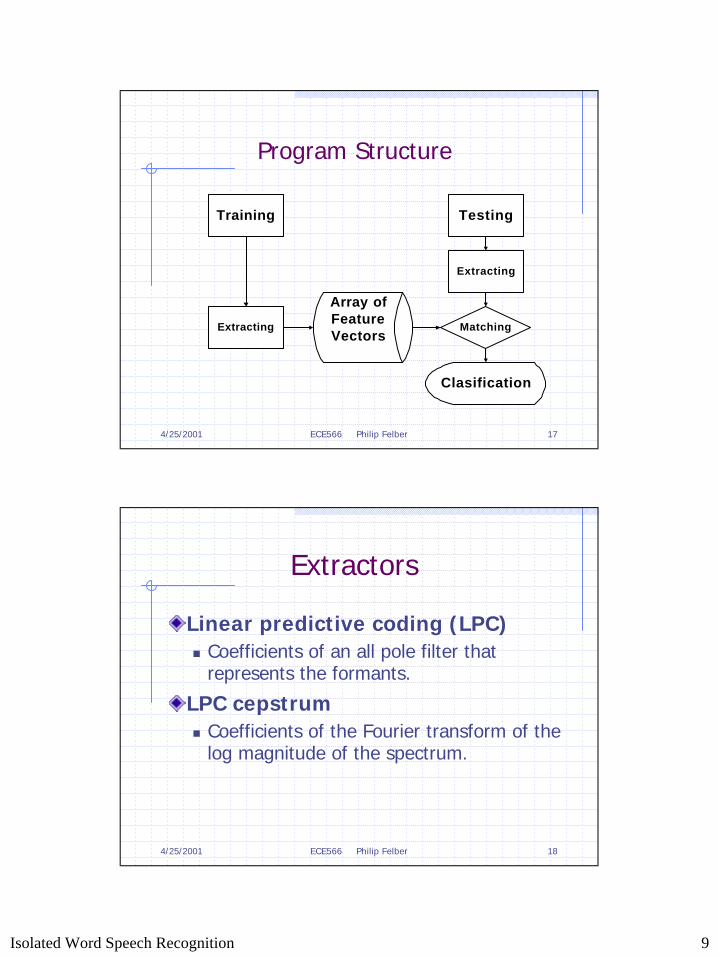
2.3. Feature extraction
Usually the features are derived from Linear Predictive Coding (LPC), a
technique that attempts to derive the coefficients of a filter that (along with a
power source) would produce the utterance that is being studied. LPC is
useful in speech processing because of its ability to extract and store time-
varying formant information. Formants are points in a sound's spectrum
where the loudness is boosted. Does the expression “all pole filter” come to
mind? What we get from LPC analysis is a set of coefficients that describe a
digital filter. The idea being that this filter in conjunction with a noise source
or a periodic signal (rich in overtones) would produce a sound similar to the
original speech. LPC data is often further processed (by recursion) to produce
what are called LPC-cepstrum features. The advantage of LPC-cepstrum
vectors (though they do not contain additional information) is that the
cepstrum vectors tend to place (in feature space) words that “sound” alike
close together. A number of advanced techniques, i.e. Dynamic Time
Warping (DTW) have been employed to improve the performance of feature
extractors. DTW is a non- linearly approach to normalizing time-scales.
2.4. Classification
A library of feature vectors is provided – a “training” process usually builds it.
The classifier uses the spectral feature set (feature vector) of the input
(unknown) word and attempts to find the “best” match from the library of

4/25/2001 ECE566 Philip Felber 10
known words. Simple classifiers, like mine, use a simple “correlation” metric
to decide. While advanced recognizers employ classifiers that utilize Hidden
Markov Models (HMM), Artificial Neural Networks (ANN), and many
others.4 The most sophisticated ASR systems search a huge database of all
“possible” sentences to find the best (most probable) match to an unknown
input.
Most of the work in the literature uses the speech production model as the
primary focus. I would also expect to find (but I did not) some researchers
approaching the problem with a model derived from the hearing process. The
use of the human voice model as opposed to the human hearing might be
explained (reasoned) by noting that the voice evolved primarily to produce
speech for conversation. Apparently hearing evolved to recognize many
sounds (including speech). In some vague sense, speaking is more specialized
than listening.
4 Jurafsky & Martin, Speech and Language Processing.

4/25/2001 ECE566 Philip Felber 11
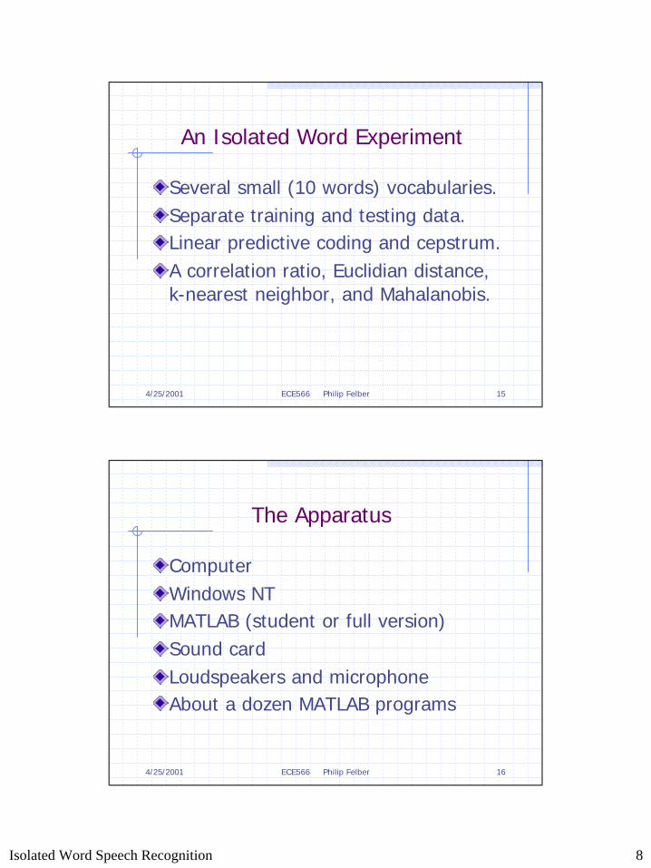
3. AN ISOLATED WORD EXPEREMENT
3.1. The apparatus
The apparatus consists of several MATLAB programs running on the Windows
operating system on a personal computer with a sound card. The programs
can be used interactively. Also, a batch facility is available to run several
experiments, with different recognition parameters, with the same input test
sample. Appendix 5.1 includes a high- level system flowchart and a detailed
flowchart of the feature extraction process. Appendix 5.2 is a complete listing
of the MATLAB programs.
Two feature extractors were employed: (1) straight LPC on the digitized (and
normalized) input, and (2) LPC-cepstrum, computed from the LPC
coefficients.
The current version of the program has four matching algorithms: (1) a
correlation measure (inner-product) between the features of the test vocabulary
(unknown) words and the averages of the features of each word from the
training sets, (2) the Euclidean distance between the features of the test word
and the averages of the words in the training sets, (3) the nonparametric
k-nearest neighbor approach (a natural extension of the single nearest or
closest), and (4) the Mahalanobis distance between the features of the test
4/25/2001 ECE566 Philip Felber 12
word and the words in the training sets. The “correlation” and the “Euclidean”
method both work averages (for each vocabulary word) of the training feature
vectors. The, nonparametric, “k-nearest” does not average the feature vectors.
Instead, it finds the (say three) nearest neighbors and then takes a plurality of
the cases. The “Mahalanobis” method5 uses the population (class) covariance
from the training data. Duda and Hart6 define the Mahalanobis distance
between x (a sample vector) and µ (the class mean or center) as r in
2 Tr -1= (x- µ) S (x-µ) . Using the inverse of the covariance matrix is intended
to account for the shape of the class cluster.
Training and testing data was collected from both male and female speakers.
One set of recordings was used for the training runs – While a different set was
used for testing.
A “script file” named batch controls the running of each experiment. It does a
standard number of trains followed by one or more individual tests. It prints
out the names of the current algorithms in use as well the values of the various
parameters that were used. Batch also accumulates and displays the standard
performance data. We use an accuracy measure that is the number of correct
answers minus the number of incorrect answers divided by the total tries times
5 Named for Prasanta Chandra Mahalanobis, the Indian physicist turned statistician who later became the
brains behind Nehru’s industrialization of India. 6 Duda and Hart, Pattern Classification and Scene Analysis.

4/25/2001 ECE566 Philip Felber 13
a hundred. This method penalizes wrong answers more severely than “don’t
know” returns.
The operating environment includes a rudimentary change or version control
facility. Doing this allows us to work with several different versions that are
in development, while a basic version that is proven is always available for
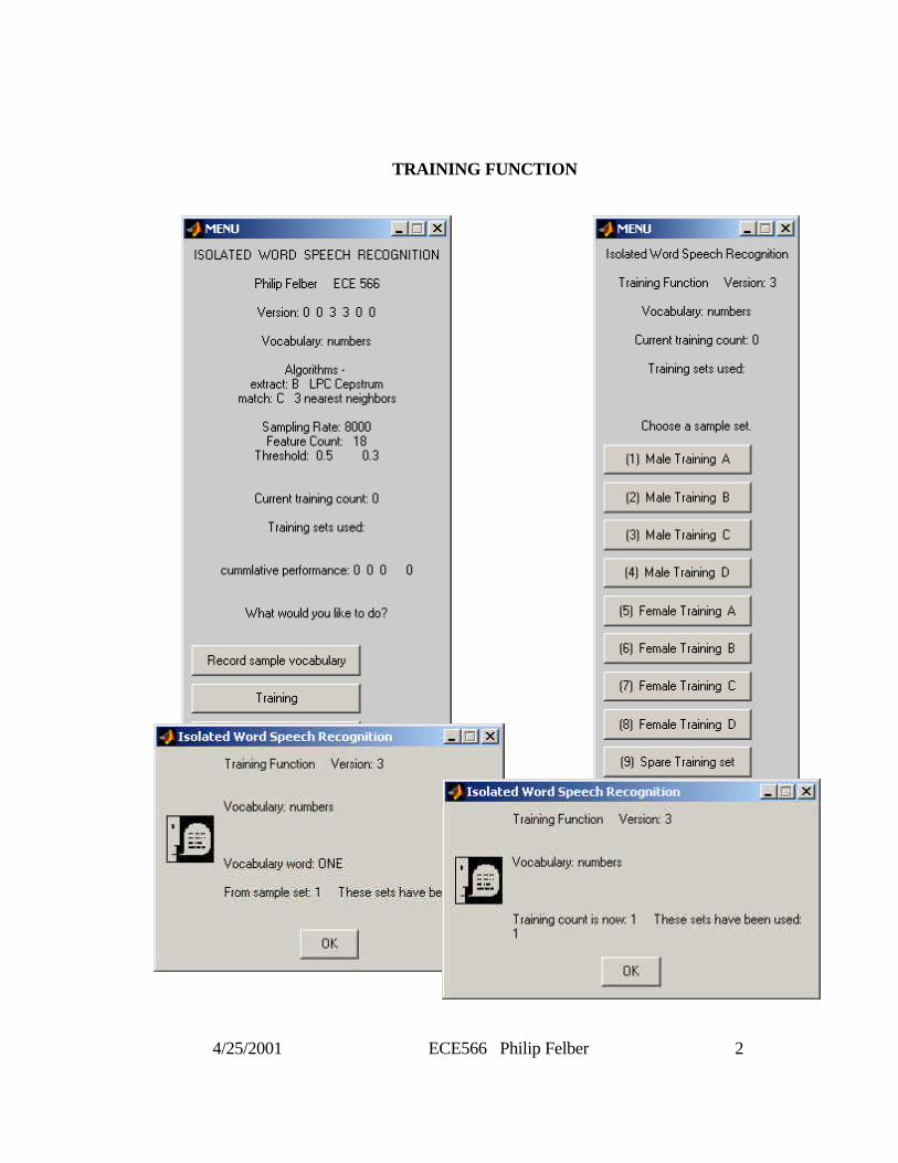
demonstrating. The main functions are training and testing, also a utility
function called recording is available to capture sample vocabulary sets for
training and testing. The training and testing programs use low-level service
routines to perform their functions. Training uses a routine named extracting
to build feature vectors. Testing uses the routine matching to develop the best
match for a test word. Like training, matching will call extracting to get the
feature vector for the test word. Matching then compares that feature vector to
the feature vectors that were developed during training. Matching then
determines the best match along with a figure of merit for that match. Testing
uses a threshold on the figures of merit returned from matching to decide if we
have a match or if we don't have enough information. So at this point testing
can say I have found a word and it is “X” or I “don’t know”. Now, from the
information as to which test word was supplied, the program knows if it is
right or wrong. Testing keeps a count of rights, wrongs and don’t knows.

4/25/2001 ECE566 Philip Felber 14
3.2. The experiments
Each experiment uses several individually recorded samples. Some are used
for training and the others are used for testing. We make a point not to test
with our training data and not to train with our testing data. The programs
allow for parameter variation and algorithm substitution for key items such as
feature extraction and class selection. The package also is designed to ga ther
and record relevant statistics on the accuracy of recognition. The general idea
is to change an algorithm and/or various controlling parameters and rerun the
standard experiment, noticing any improvement or degradation in the statistics
that represent successful recognition. The results that I report are from runs
(experiments) using two voices (one male and one female). Each speaker
recorded eight tapes (four to be use for training and four to be used for testing).
Each tape is a complete pass through the vocabulary words. We used the
digits one through nine and zero but any small vocabulary could be used. We
considered colors, i.e. ‘red’, ‘green’, ‘blue’, and the rest, also names, i.e.
‘John’, ‘Mary’, ‘Henry’, ‘Robin’, ‘Philip’, ‘Karen’, and the like. Partway
through the project I added a second vocabulary (to demonstrate the versatility
of the programs). This second vocabulary is somewhat artificial as it contains
the long vowel sounds, a few colors plus ‘yes’ and ‘no’. A “run”, for

4/25/2001 ECE566 Philip Felber 15
performance measurement against a specific algorithm and parameter setup,
consisted of playing eight training tapes (four male and four female) followed
by the remaining eight testing tapes. For each test tape, performance data
(rights, wrongs and don’t knows) is captured. After all eight testing tapes are
played the performance data is summarized into a single rating. Again, the
measure that was used is: add one point for each correct match; subtract one
for each wrong answer (don’t knows don’t count either way) and then convert
to a percent. This approach allows us to develop a recognizer that would
rather ask for a repeat than make an error.
4/25/2001 ECE566 Philip Felber 16
3.3. The results
An appendix (5.4) contains batch runs for the various algorithm
combinations. All of the relevant results of my experiments are also tabulated
in this appendix.
Two vocabularies were used in the experiments. “Numbers” is a ten word
vocabulary composed of the spoken digits: one, two, three, four, five, six,
seven, eight, nine, and zero. “Aeiou” is an artificial set composed of the
long vowel sounds: A, E, I, O, and U. To these vowel sounds I added these
familiar words: red, green, blue, yes, and no.
This data is for a combination of two speakers (one male and one female).
Each of the sixteen runs (two feature extractors vs. four class matchers for
each of the two vocabularies) consisted of eight trainings followed by eight
“testings”. Thirty-two, individually recorded, tapes were used - Eight training
and eight testing for each of two vocabularies. Each tape contains one
utterance of each of the ten vocabulary words.

4/25/2001 ECE566 Philip Felber 17
4. SUMMARY
Generally, linear prediction worked better than LPC-cepstrum. I would expect
LPC-cepstrum to be better than LPC if used on individual phonemes (as
opposed to complete words).
Laboratory (controlled environment) was better than studio (general use).
The poor performance of the Mahalanobis method is thought to be a result of
my small number of training sets. With just a few trainings (I used eight) for
each class I do get a very good handle on the class mean, but since I need so
many features (in the high teens), I for sure can expect trouble with the
covariance matrix! I needed to reduce my feature count to nine to be
consistent with my eight training samples. Remember, my features are the
filter coefficients (not the poles); therefore my nine features contain at most
eight degrees of freedom. I modified the MATLAB routine mahala to use
pseudoinverse (pinv) to avoid the fatal error in inverse (inv) whenever the
covariance matrix turns out to be singular.
As one might expect, a good noise-canceling microphone improves
performance.

5. APPENDIXES
5.1. Program Flowcharts
Overview of training and testing page 1
Preprocessing and feature extracting page 2

4/25/2001 ECE566 Philip Felber 1

4/25/2001 ECE566 Philip Felber 2
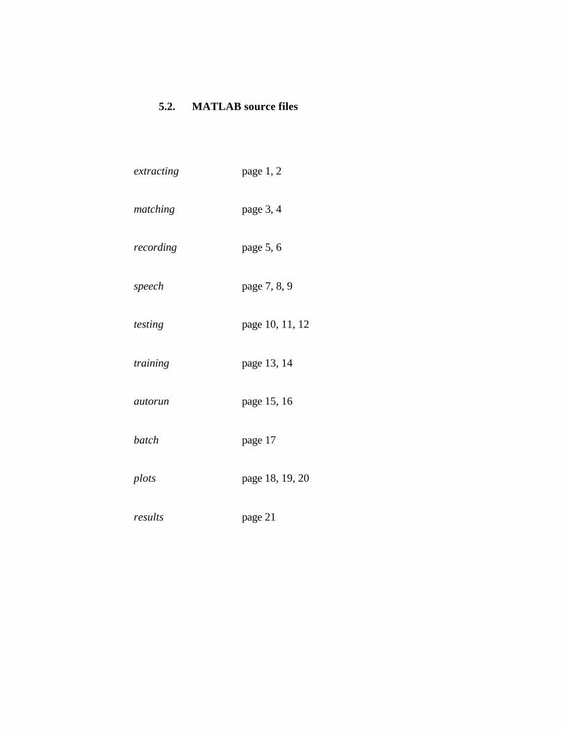
5.2. MATLAB source files
extracting page 1, 2
matching page 3, 4
recording page 5, 6
speech page 7, 8, 9
testing page 10, 11, 12
training page 13, 14
autorun page 15, 16
batch page 17
plots page 18, 19, 20
results page 21
extracting.mApril 25, 2001
Page 18:58:40 PM
function features = extracting(W,data)% feature extraction% called by matching and training% returns feature vector for a sampled word input%global Names Words Feat Cls Fs Fn Tn Tries Thres Test V First Alg St K Vocv = 4; % Version 3-29-01V(1) = v;if Test disp([' extracting(',num2str(W),',data) Ver: ',num2str(v)]);endif sum(Alg{1,1}~='extract'), disp(['error - improper Alg']); pause; endfs = length(data); % sampling rate for this samplesample = double(data);sample = sample - mean(sample); % remove DC componentswitch Alg{1,2} % algorithm code: A,B,... case 'A' % Linear Prediction sample = filter([1 -0.97],[1 0.53],sample); % pre-filter case 'B' % LPC cepstrum sample = filter([1 -0.945],[1],sample); % pre-emphasis filter otherwise disp('Unknown method.');endsample = sample/max(abs(sample)); % standard amplitude% note Fs = 8000 | 11025 | 22050 | 44100wz = 25; % window size for time alignment (works for all FS)wc = fs/wz; % window countws = [1:wz:fs]; % start of each windowwe = [wz:wz:fs]; % end of each windowtc = 0;for n=1:wc energy(n) = sample(ws(n):we(n))'*sample(ws(n):we(n)); tc = tc+n*energy(n);endtc = round(tc/wc/mean(energy(1:wc))); % time center of energytcwz = tc*wz; % computed time center for signaladj = round(fs/2-tcwz); % alignment amountif adj<0 % negative move left, positive move right, zero leave alone sample = [sample([-adj:fs],1);zeros(-adj-1,1)];elseif adj>0 sample = [zeros(adj-1,1);sample([1:fs-adj,1])];endswitch Alg{1,2} % algorithm code: A,B,... case 'A' % Linear Prediction [Lfeatures,Power] = lpc(sample,Fn-1); % Linear Predictor Coeff. Lfeatures = real(Lfeatures); % real part features = Lfeatures; case 'B' % LPC cepstrum [Lfeatures,Power] = lpc(sample,Fn-1); % Linear Predictor Coeff.

extracting.mApril 25, 2001
Page 28:58:41 PM
[Cfeatures,yh] = rceps(Lfeatures); % real cepstrum of LPC features = Cfeatures; otherwise disp('Unknown method.');endif Test disp([' power: ',num2str(Power),' length: '... ,num2str(length(sample))]); figure if W~=0, name = Names{W}; else, name = 'test'; end subplot(221); plot(data); title(name); subplot(222); plot(sample); title('Standardize '); subplot(223); stem(1:length(Lfeatures),Lfeatures); title('LPC'); if exist('Cfeatures') subplot(224); stem(1:length(Cfeatures),Cfeatures); title('LPC cepstrum'); end pauseend
matching.mApril 25, 2001
Page 39:28:35 PM
function [word, match] = matching(W,testdata)% picks best choice% called by "testing"% calls "extracting"% returns word number and match quality%global Names Words Feat Cls Fs Fn Tn Tries Thres Test V First Alg St K Vocv = 4; % Version 4-19-01V(2) = v;if Test, disp([' matching(testdata) Ver: ',num2str(v)]), endif sum(Alg{2,1}~='match'), disp(['error - improper Alg']); pause; endy = extracting(W,testdata); % get feature vector for test wordswitch Alg{2,2} % algorithm code: A,B,...case 'A' % calculate match using correlation ratio if Test, disp([' calculate match using correlation ratio']), end for m=1:length(Names) % each vocabulary word x = sum(Feat(find(Cls==m),:),1)/Tn; % average feature vector R(m) = normr(x) * normc(y'); % Correlation endcase 'B' % calculate match using Euclidean distance if Test, disp([' calculate match using Euclidean dist']), end for m=1:length(Names) % each vocabulary word x = sum(Feat(find(Cls==m),:),1)/Tn; % average feature vector R(m) = sqrt(sum((x-y).^2,2)); % Euclidean distance end R = normr(1./R); % normalize match coefcase 'C' % calculate match using k nearest neighbor if Test, disp([' calculate match using k nearest']), end for n=1:size(Feat,1) % for each feature vector x = Feat(n,:); % one feature vector D(n) = sqrt(sum((x-y).^2,2)); % Euclidean distance end R = sortrows([D',Cls'],1); T1 = tabulate(R(1:K,2)); % K is k of k-nearest T2 = tabulate(R(1:K+1,2)); if max(T1(:,2))<max(T2(:,2)) T = abs(sortrows(-T2,3)); else T = abs(sortrows(-T1,3)); endcase 'D' % Mahalanobis distance if Test, disp([' calculate match using Mahalanobis dist']), end % class = classify(y(:,2:Fn),Feat(:,2:Fn),Cls'); for m=1:length(Names) % each vocabulary word % pmahal is a rework of builtin mahal using pseudo inverse R(m) = pmahal(y(:,2:Fn),Feat(find(Cls==m),2:Fn)); % Mahalanobis end R = normr(1./R); % normalize match coefotherwise

matching.mApril 25, 2001
Page 49:28:35 PM
disp('Unknown method.');endswitch Alg{2,2} % algorithm codecase {'A','B','D'} % correlation ratio | Euclidean dist | Mahalanobis [match(1),word] = max(R); % Match coef for chosen word RR = R; RR(word) = 0; % find coef for second best word match(2) = (match(1) - max(RR)); % Match margin if Test, disp([' ',num2str(R(1:5))]); end if Test, disp([' ',num2str(R(6:10))]); end if Test, disp([' ',num2str(word),' ',num2str(match)]); endcase 'C' % k nearest neighbor word = T(1,1); if size(T,1)<2, T(2,3) = 0; end match = [T(1,3)/100,(T(1,3)-T(2,3))/100]; if Test, disp(T); endotherwise disp('Unknown method.');end
recording.mApril 25, 2001
Page 58:58:59 PM
function recording% records vocabulary sets as sample#.mat (#=1,9)%global Names Words Feat Cls Fs Fn Tn Tries Thres Test V First Alg St K Vocv = 3; % Version 3-14-01V(3) = v;if Test, disp([' recording Ver: ',num2str(v)]), endsample = cell(1,length(Names));M = menu({'Isolated Word Speech Recognition',' '... ,['Recording Function Version: ',num2str(v)],' '... ,'Choose data type.'}... ,'Training Data.'... ,'Testing Data.'... ,'quit');if M==1, DT = ['Training Data\',Voc]; endif M==2, DT = ['Testing Data\',Voc]; end if M==3, return; end M = menu({'Isolated Word Speech Recognition',' '... ,['Recording Function Version: ',num2str(v)],' '... ,['You are working with: ',DT],' '... ,'What would you like to do?'}... ,'Record a new vocabulary sample set.'... ,'Enter a label for an existing sample set.'... ,'quit');if M==3, return; end if M==2 filename = [DT,'\voice']; load(filename,'voice'); while 1 U = menu({'Isolated Word Speech Recognition',' '... ,['Recording Function Version: ',num2str(v)],' '... ,['You are working with: ',DT],' '... ,'Which sample set would you like to label?'}... ,['(1) ',voice{1}],['(2) ',voice{2}],['(3) ',voice{3}]... ,['(4) ',voice{4}],['(5) ',voice{5}],['(6) ',voice{6}]... ,['(7) ',voice{7}],['(8) ',voice{8}],['(9) ',voice{9}]... ,'quit'); if U==10, break; end voice{U} = input(['Enter name for ',DT,' set: '... ,num2str(U),' >'],'s'); end filename = [DT,'\voice']; save(filename,'voice'); return;endwhile 1% listen to one set of vocabulary wordsmsgbox({['Recording Function Version: ',num2str(v)],' ',' '... ,[DT,' Preparation. Say each vocabulary word after the prompt.']}... ,'Isolated Word Speech Recognition','help','replace');beep;

recording.mApril 25, 2001
Page 68:58:59 PM
pause(3);for N = 1:length(Names) msgbox({['Recording Function Version: ',num2str(v)],' ',' '... ,[DT,' Set ACTION. Say the word!',' ',Names{N}],' ',' '... ,[' !!! ',Names{N},' !!!']}... ,'Isolated Word Speech Recognition','help','replace'); pause(0.2) sample{N} = wavrecord(1*Fs,Fs,1,'double'); wavplay(sample{N},length(sample{N})); close all hidden;endfilename = [DT,'\voice']; load(filename,'voice');M = menu({'Isolated Word Speech Recognition',' '... ,['Recording Function Version: ',num2str(v)],' '... ,['You are working with: ',DT],' '... ,'Choose a label for this sample set.'}... ,['(1) ',voice{1}],['(2) ',voice{2}],['(3) ',voice{3}]... ,['(4) ',voice{4}],['(5) ',voice{5}],['(6) ',voice{6}]... ,['(7) ',voice{7}],['(8) ',voice{8}],['(9) ',voice{9}]... ,'quit');if M==10, return; endfilename = [DT,'\sample',num2str(M)]; save(filename, 'sample');M = menu({'Isolated Word Speech Recognition',' '... ,['Recording Function Version: ',num2str(v)],' '... ,['You are working with: ',DT]}... ,'Record a vocabulary sample.'... ,'quit');if M==2, return; endpause(2);end
speech.mApril 25, 2001
Page 79:33:38 PM
%this is the mainline for ECE566 isolated word recognition by Philip Felber% function calls - program names and code numbers% % speech(4)-----.--->recording(3)% |% |--->training(6)------>extracting(1)% |% |--->testing(5)------->matching(2)------>extracting(1)%%% algorithms: EXTRACT - A: Linear Prediction% B: LPC Cepstrum%% MATCH - A: Correlation ratio % B: Euclidean distance% C: k-nearest neighbor% D: Mahalanobis distance%cd('y:\ece566\speech');global Names Words Feat Cls Fs Fn Tn Tries Thres Test V First Alg St K Vocv = 3; % Version 3-12-01if isempty(Test), Test = 0; end % debugging flagif isempty(First), First = 1; end % start upTries = zeros(1,3); % count of tries: ["yes","no","don't know"]tries = Tries; % local accumulator for rolling performanceperformance = 0;if isempty(Fn), First = 1; Fn = 18; end % Feature countif isempty(Fs), First = 1; Fs=[8000, 11025, 22050, 44100]; Fs=Fs(1); endif isempty(Thres), First = 1; Thres = [0.5, 0.300]; endif isempty(Voc), First = 1; Voc = 'numbers'; end % aeiou | numbersif isempty(Alg), First = 1; Alg{1,2} = 'B'; Alg{2,2} = 'C'; endif First First = 0; St =[]; % used training sets V = zeros(1,6); V(4) = v; % version if isempty(Alg), Alg{1,2} = 'B'; Alg{2,2} = 'C'; end Alg{1,1} = 'extract'; Alg{2,1} = 'match'; Tn = 0; % training countif length(Voc)==7 % numbers Names = {'ONE','TWO','THREE','FOUR','FIVE'... ,'SIX','SEVEN','EIGHT','NINE','ZERO'};elseif length(Voc)==5 % aeiou Names = {'A','E','I','O','U'... ,'RED','GREEN','BLUE','YES','NO'};end Words = cell(1,length(Names)); Feat = zeros(0,Fn); % feature vector for each training sample Cls = zeros(1,0); % class for each training sample Go = 0;

speech.mApril 25, 2001
Page 89:33:38 PM
else Go = 1;endswitch Alg{1,2} case 'A' Alg{1,3} = 'Linear Prediction'; case 'B' Alg{1,3} = 'LPC Cepstrum'; otherwise disp('Unknown method.'); return;end switch Alg{2,2} case 'A' Alg{2,3} = 'Correlation ratio'; case 'B' Alg{2,3} = 'Euclidean distance'; case 'C' if isempty(K), K = 3; end Alg{2,3} = strcat(num2str(K),' nearest neighbors'); case 'D' Alg{2,3} = 'Mahalanobis dist'; otherwise disp('Unknown method.'); returnend while Go M = menu({'ISOLATED WORD SPEECH RECOGNITION',' '... ,'Philip Felber ECE 566',' '... ,['Version: ',num2str(V)],' ',['Vocabulary: ', Voc],' '... ,['Algorithms - '],[Alg{1,1},': ',Alg{1,2},' ',Alg{1,3}]... ,[Alg{2,1},': ',Alg{2,2},' ',Alg{2,3}],' '... ,['Sampling Rate: ',num2str(Fs)]... ,['Feature Count: ',num2str(Fn)]... ,['Threshold: ',num2str(Thres)],' ',' '... ,['Current training count: ',num2str(Tn)],' '... ,['Training sets used:'], [num2str(St)],' '... ,['cummlative performance: ',num2str(tries),' '... ,num2str(performance)],' ',' ','What would you like to do?'... ,' '},'Record sample vocabulary','Training','Testing'... ,'Toggle "debug" flag','Quit'); close all hidden; switch M case 1 % 'Record sample words' recording; case 2 % 'Training' training; case 3 % 'Testing' testing;

speech.mApril 25, 2001
Page 99:33:38 PM
tries = tries + Tries; % Roll totals if sum(tries)==0 performance = 0; else performance = 100*(tries(1)-tries(2))/sum(tries); end case 4 % 'Toggle "debug" flag' Test = Test==0; disp(['Test = ',num2str(Test)]); otherwise % quit break; end end

testing.mApril 25, 2001
Page 108:59:17 PM
function testing(T)% Guess the name of word in the test input% calls "matching"%global Names Words Feat Cls Fs Fn Tn Tries Thres Test V First Alg St K Vocv = 3; % Version 3-14-01V(5) = v; % versionif ~exist('T'), T = 0; endif Test, disp([' testing(',num2str(T),') Ver: ',num2str(v)]), endif Tn==0 msgbox({['Testing Function Version: ',num2str(v)],' ',' '... ,'Operational sequence error. Current traning count is ZERO!'}... ,'Isolated Word Speech Recognition','help','replace'); beep; pause(1); return;endTries=zeros(size(Tries)); % reset performance countersDT = ['Testing Data\',Voc];if T==0 filename = [DT,'\voice']; load(filename,'voice'); voice{10}='Microphone'; S = menu({'Isolated Word Speech Recognition',' '... ,['Testing Function Version: ',num2str(v)],' ',' '... ,['Vocabulary: ', Voc],' '... ,['Current training count: ',num2str(Tn)],' '... ,['Training sets used:'], [num2str(St)],' ',' '... ,['Choose a sample set.']}... ,['(1) ',voice{1}],['(2) ',voice{2}],['(3) ',voice{3}]... ,['(4) ',voice{4}],['(5) ',voice{5}],['(6) ',voice{6}]... ,['(7) ',voice{7}],['(8) ',voice{8}],['(9) ',voice{9}]... ,['(10) ',voice{10}],'quit');else S = T;endif S==11, close all hidden; return; endif S~=10 filename = [DT,'\sample',num2str(S)]; load(filename, 'sample');endfor loop=1:length(Names) if S~=10 testdata = sample{loop}; [word, match] = matching(loop,testdata); if sum(match > Thres)>1 if T==0, wavplay(testdata,length(testdata)); end if word==loop Tries(1) = Tries(1) + 1; % count "rights" else Tries(2) = Tries(2) + 1; % count "wrongs" end

testing.mApril 25, 2001
Page 118:59:18 PM
else if T==0, wavplay(testdata,length(testdata)); end Tries(3) = Tries(3) + 1; % count "don't knows" end else msgbox({['Testing Function Version: ',num2str(v)],' ',' '... ,['Vocabulary: ', Voc],' '... ,'Say a test word after the prompt.'}... ,'Isolated Word Speech Recognition','help','replace'); pause(1); beep; pause(0.5); msg = msgbox({['Testing Function Version: ',num2str(v)]... ,' ',' ',' ',' ',' '... ,' !!! NOW !!!'}... ,'Isolated Word Speech Recognition'... ,'help','replace'); pause(0.3); testdata = wavrecord(1*Fs,Fs,1,'double'); pause(0.3); close(msg); [word, match] = matching(0,testdata); if sum(match > Thres)>1 wavplay(testdata,length(testdata)); M = menu({'Isolated Word Speech Recognition',' '... ,['Testing Function Version: ',num2str(v)],' ',' '... ,['Vocabulary: ', Voc],' '... ,['Did you say? ',Names{word}],' '... ,[' Match coef & margin: ',num2str(match)]}... ,'yes','no','quit'); if M==3, loop = 0; end Tries(M) = Tries(M) + 1; % count "rights" and "wrongs" else wavplay(testdata,length(testdata)); M = menu({'Isolated Word Speech Recognition',' '... ,['Testing Function Version: ',num2str(v)],' ',' '... ,['Vocabulary: ', Voc],' '... ,['Do not understand! Match margin: '... ,num2str(match),' ',num2str(word)]},'continue','quit'); if M==2, loop = 0; end Tries(3) = Tries(3) + 1; % accumulate count of "don't knows" end end performance = 100*(Tries(1)-Tries(2))/sum(Tries); % calc performance if loop==0, return; end if T==0 msgbox({['Testing Function Version: ',num2str(v)],' ',' '... ,['Match and Margin: ',num2str(match),' '... ,Names{word}],' ',' '... ,['Set: ',num2str(S),' ',voice{S}],' ',['Word: '... ,Names{loop},' Tries: ',num2str(Tries)]... ,['Performance (right''s - wrong''s): '... ,num2str(round(performance))]}...

testing.mApril 25, 2001
Page 128:59:18 PM
,'Isolated Word Speech Recognition','help','replace'); if loop~=length(Names), pause(2); else, pause(3); end end if loop==0, close all hidden; return; endend
training.mApril 25, 2001
Page 138:59:25 PM
function training(T)% collects data for the vocabulary% calls "extracting"%global Names Words Feat Cls Fs Fn Tn Tries Thres Test V First Alg St K Vocv = 3; % Version 3-12-01V(6) = v;if ~exist('T'), T = 0; endif Test, disp([' training(',num2str(T),') Ver: ',num2str(v)]), endDT = ['Training Data\',Voc];% load one set of vocabulary words from training dataif T~=0 M = T;else filename = [DT,'\voice']; load(filename,'voice'); M = menu({'Isolated Word Speech Recognition',' '... ,['Training Function Version: ',num2str(v)],' '... ,['Vocabulary: ', Voc],' '... ,['Current training count: ',num2str(Tn)],' '... ,['Training sets used:'], [num2str(St)],' ',' '... ,'Choose a sample set.'}... ,['(1) ',voice{1}],['(2) ',voice{2}],['(3) ',voice{3}]... ,['(4) ',voice{4}],['(5) ',voice{5}],['(6) ',voice{6}]... ,['(7) ',voice{7}],['(8) ',voice{8}],['(9) ',voice{9}]... ,'quit'); if M==10, return; endendfilename = [DT,'\sample',num2str(M)]; load(filename, 'sample');% build features for training datafor N=1:length(Names) if N==length(Names) Tn = Tn + 1; % bump training count St = sort([St,M]); % used training sets end Words{N} = sample{N}; % move sample to active Feat(length(Cls)+1,:) = extracting(N,Words{N}); % feature vector Cls(length(Cls)+1) = N; % class for this training sample if T==0 msgbox({['Training Function Version: ',num2str(v)]... ,' ',' ',['Vocabulary: ', Voc],' '... ,' ',' ',['Vocabulary word: ',Names{N}],' '... ,['From sample set: ',num2str(M)... ,' These sets have been used:'], num2str(St)}... ,'Isolated Word Speech Recognition'... ,'help','replace'); pause(0.1); wavplay(Words{N},length(Words{N})); % sound each training word close all hidden; end

training.mApril 25, 2001
Page 148:59:25 PM
end if T==0 msgbox({['Training Function Version: ',num2str(v)]... ,' ',' ',['Vocabulary: ', Voc],' '... ,' ',' ',['Training count is now: ',num2str(Tn)... ,' These sets have been used:'],num2str(St)}... ,'Isolated Word Speech Recognition','help','replace'); pause(3);end
autorun.mApril 25, 2001
Page 158:59:33 PM
% autorun% load training datacd('y:\ece566\speech');close all hiddenclear allglobal Names Words Feat Cls Fs Fn Tn Tries Thres Test V First Alg St K Voc Fn = 18; % Feature Count > 3Thres = [0.5, 0.3]; % Threshold [match, margin] Alg{1,2} = 'B'; % extract - Linear Prediction | LPC cepstrumAlg{2,2} = 'C'; % match - correlation | Euclidean dist | k nearestK =3; % k of k-nearestVoc = 'numbers'; % aeiou | numbersspeech; % initializationfilename = ['Training Data\',Voc,'\voice']; load(filename,'voice');for T=1:8, training(T); disp([voice(T)]); endtries = zeros(1,2);filename = ['Testing Data\',Voc,'\voice']; load(filename,'voice');for S=1:8 filename = ['Testing Data\',Voc,'\sample',num2str(S)]; load(filename, 'sample'); Sample{S} = sample;end loop = 100;while loop>0 S = ceil(8*rand); W = ceil(10*rand); sample = Sample{S}; testdata = sample{W}; wavplay(testdata,length(testdata)); [word, match] = matching(W,testdata); tries(~(W==word)+1) = tries(~(W==word)+1) + 1; % cnt rights & wrongs if W==word, Quess = 'RIGHT'; else, Quess = 'WRONG'; end msg = msgbox... ({'Autorun Function - Random words from random test sets.'... ,' ',['Vocabulary: ', Voc(2:length(Voc))],' '... ,['Algorithms - '],[Alg{1,1},': ',Alg{1,2},' ',Alg{1,3}]... ,[Alg{2,1},': ',Alg{2,2},' ',Alg{2,3}],' '... ,['Sampling Rate: ',num2str(Fs)]... ,['Feature Count: ',num2str(Fn)]... ,['Threshold: ',num2str(Thres)],' ',' '... ,['Current training count: ',num2str(Tn)],' '... ,['Training sets used:'], [num2str(St)],' '... ,['Selected Test Set: ',voice{S}],' ',' '... ,[' Selected word: ',Names{W}],' ',' '... ,['Matched Class: ',Names{word},' ',num2str(mod(word,10))... ,' Confidence: ',num2str(match(1))],' ',' '... ,[' ',Quess],' ',' '... ,['Performance(right, wrong): ',num2str(tries),' '... ,num2str(100*tries(1)/sum(tries,2))]}... ,'Isolated Word Speech Recognition'... ,'help','replace'); pause(2); loop = loop - 1;

autorun.mApril 25, 2001
Page 168:59:33 PM
if mod(loop,10)==0 M = menu({'Isolated Word Speech Recognition',' '... ,' Continue with 10 more tries?'}... ,'yes','no'); if M==2, loop = 0; end end end

batch.mApril 25, 2001
Page 178:59:41 PM
function Sum = batch(ext,mat,fn,thres)% This is a script, used to run multiple studies% 3 % Version 3-15-01cd('y:\ece566\speech');R=[1:8]; % range for this rundisp([ext,' ',mat,' ',num2str(fn),' ',num2str(thres)]);
clear globalglobal Names Words Feat Cls Fs Fn Tn Tries Thres Test V First Alg St K Voc Fn = fn; % Feature Count > 3Thres = thres; % Threshold [match, margin] Alg{1,2} = ext; % extract - Linear Prediction | LPC cepstrumAlg{2,2} = mat; % match - correl. | Euclidean | k nearest | MahalanobisK =3; % k of k-nearestVoc = 'numbers'; % aeiou | numbers
disp(' '); disp([date,' Vocabulary: ',Voc]); disp(' '); speech; % initialization filename = ['Training Data\',Voc,'\voice']; load(filename,'voice'); for T=R, training(T); disp([voice(T)]); end disp(['Training count: ',num2str(Tn),' Right, Wrong, Don''t know',]);disp(' '); filename = ['Testing Data\',Voc,'\voice']; load(filename,'voice');
for S=[1:8] testing(S); results(S,:) = Tries; disp({char(voice(S)),num2str(results(S,:))});end
Sum = sum(results,1); disp(['Sum = ',num2str(Sum),' '... ,'Performance (right''s - wrong''s) = '... ,num2str(100*(Sum(1)-Sum(2))/sum(Sum,2))]); disp(' ');disp(['Version: ',num2str(V)]); disp(' '); % versionsdisp(['Sample Rate: ',num2str(Fs),' Feature Count: ',num2str(Fn)... ,' Threshold: ',num2str(Thres)]); disp(' ');disp('Algorithms - '); disp(Alg); disp(' ');
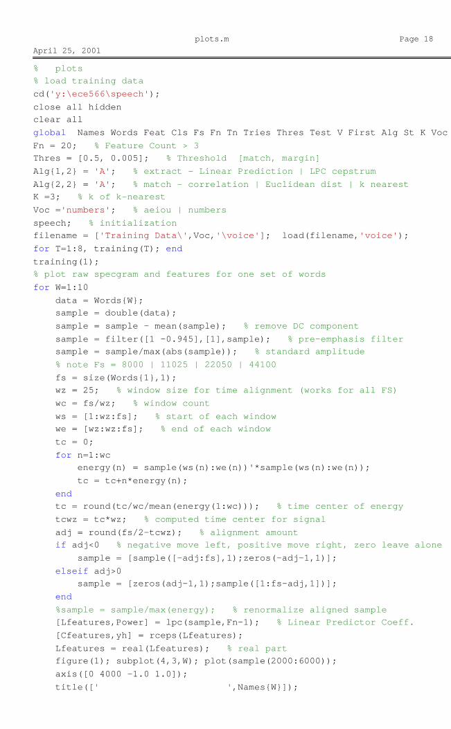
plots.mApril 25, 2001
Page 189:40:31 PM
% plots% load training datacd('y:\ece566\speech');close all hiddenclear allglobal Names Words Feat Cls Fs Fn Tn Tries Thres Test V First Alg St K Voc Fn = 20; % Feature Count > 3Thres = [0.5, 0.005]; % Threshold [match, margin] Alg{1,2} = 'A'; % extract - Linear Prediction | LPC cepstrumAlg{2,2} = 'A'; % match - correlation | Euclidean dist | k nearestK =3; % k of k-nearestVoc ='numbers'; % aeiou | numbersspeech; % initialization filename = ['Training Data\',Voc,'\voice']; load(filename,'voice'); for T=1:8, training(T); endtraining(1);% plot raw specgram and features for one set of wordsfor W=1:10 data = Words{W}; sample = double(data); sample = sample - mean(sample); % remove DC component sample = filter([1 -0.945],[1],sample); % pre-emphasis filter sample = sample/max(abs(sample)); % standard amplitude % note Fs = 8000 | 11025 | 22050 | 44100 fs = size(Words{1},1); wz = 25; % window size for time alignment (works for all FS) wc = fs/wz; % window count ws = [1:wz:fs]; % start of each window we = [wz:wz:fs]; % end of each window tc = 0; for n=1:wc energy(n) = sample(ws(n):we(n))'*sample(ws(n):we(n)); tc = tc+n*energy(n); end tc = round(tc/wc/mean(energy(1:wc))); % time center of energy tcwz = tc*wz; % computed time center for signal adj = round(fs/2-tcwz); % alignment amount if adj<0 % negative move left, positive move right, zero leave alone sample = [sample([-adj:fs],1);zeros(-adj-1,1)]; elseif adj>0 sample = [zeros(adj-1,1);sample([1:fs-adj,1])]; end %sample = sample/max(energy); % renormalize aligned sample [Lfeatures,Power] = lpc(sample,Fn-1); % Linear Predictor Coeff. [Cfeatures,yh] = rceps(Lfeatures); Lfeatures = real(Lfeatures); % real part figure(1); subplot(4,3,W); plot(sample(2000:6000)); axis([0 4000 -1.0 1.0]); title([' ',Names{W}]);
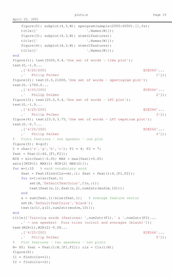
plots.mApril 25, 2001
Page 199:40:31 PM
figure(2); subplot(4,3,W); specgram(sample(2000:6000),[],fs); title([' ',Names{W}]); figure(3); subplot(4,3,W); stem(Lfeatures); title([' ',Names{W}]); figure(4); subplot(4,3,W); stem(Cfeatures); title([' ',Names{W}]);endfigure(1); text(5000,9.4,'One set of words - time plot');text(0,-1.9... ,['4/25/2001 ECE566'... ,' Philip Felber 1']);figure(2); text(0.5,21000,'One set of words - spectogram plot');text(0,-1700.0... ,['4/25/2001 ECE566'... ,' Philip Felber 2']);figure(3); text(25.0,9.4,'One set of words - LPC plot');text(0,-1.9... ,['4/25/2001 ECE566'... ,' Philip Felber 3']);figure(4); text(23.0,3.75,'One set of words - LPC cepstrum plot');text(0,-0.7... ,['4/25/2001 ECE566'... ,' Philip Felber 4']);% Plots features - one speaker - one plotfigure(5); H=gcf;C = char('r','g','b','c'); F1 = 4; F2 = 7;feat = Feat(1:40,[F1,F2]);MIN = min(feat)-0.05; MAX = max(feat)+0.05;axis([MIN(1) MAX(1) MIN(2) MAX(2)]);for m=1:10 % each vocabulary word feat = Feat(find(Cls==m),:); feat = feat(1:4,[F1,F2]); for n=1:size(feat,1) set(H,'DefaultTextColor',C(n,:)); text(feat(n,1),feat(n,2),num2str(mod(m,10))); end x = sum(feat,1)/size(feat,1); % average feature vector set(H,'DefaultTextColor','black'); text(x(1),x(2),num2str(mod(m,10)));endtitle(['Training words (features: ',num2str(F1),' & ',num2str(F2)... ,' - one speaker) Four tries (color) and averages (black)']);text(MIN(1),MIN(2)-0.08... ,['4/25/2001 ECE566'... ,' Philip Felber 5']);% Plot features - two speakers - ten plotsN= 80; feat = Feat(1:N,[F1,F2]); cls = Cls(1:N);figure(6);I1 = find(cls==1);I2 = find(cls==2);
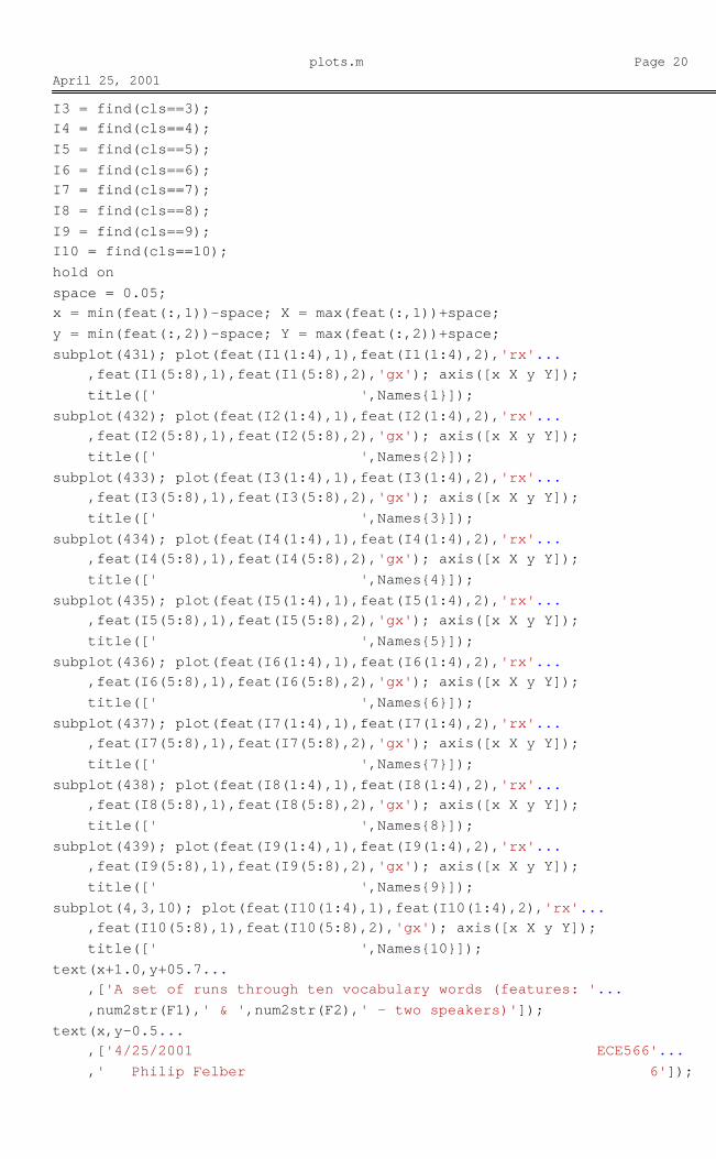
plots.mApril 25, 2001
Page 209:40:31 PM
I3 = find(cls==3);I4 = find(cls==4);I5 = find(cls==5);I6 = find(cls==6);I7 = find(cls==7);I8 = find(cls==8);I9 = find(cls==9);I10 = find(cls==10);hold onspace = 0.05;x = min(feat(:,1))-space; X = max(feat(:,1))+space;y = min(feat(:,2))-space; Y = max(feat(:,2))+space;subplot(431); plot(feat(I1(1:4),1),feat(I1(1:4),2),'rx'... ,feat(I1(5:8),1),feat(I1(5:8),2),'gx'); axis([x X y Y]); title([' ',Names{1}]);subplot(432); plot(feat(I2(1:4),1),feat(I2(1:4),2),'rx'... ,feat(I2(5:8),1),feat(I2(5:8),2),'gx'); axis([x X y Y]); title([' ',Names{2}]); subplot(433); plot(feat(I3(1:4),1),feat(I3(1:4),2),'rx'... ,feat(I3(5:8),1),feat(I3(5:8),2),'gx'); axis([x X y Y]); title([' ',Names{3}]); subplot(434); plot(feat(I4(1:4),1),feat(I4(1:4),2),'rx'... ,feat(I4(5:8),1),feat(I4(5:8),2),'gx'); axis([x X y Y]); title([' ',Names{4}]); subplot(435); plot(feat(I5(1:4),1),feat(I5(1:4),2),'rx'... ,feat(I5(5:8),1),feat(I5(5:8),2),'gx'); axis([x X y Y]); title([' ',Names{5}]); subplot(436); plot(feat(I6(1:4),1),feat(I6(1:4),2),'rx'... ,feat(I6(5:8),1),feat(I6(5:8),2),'gx'); axis([x X y Y]); title([' ',Names{6}]); subplot(437); plot(feat(I7(1:4),1),feat(I7(1:4),2),'rx'... ,feat(I7(5:8),1),feat(I7(5:8),2),'gx'); axis([x X y Y]); title([' ',Names{7}]); subplot(438); plot(feat(I8(1:4),1),feat(I8(1:4),2),'rx'... ,feat(I8(5:8),1),feat(I8(5:8),2),'gx'); axis([x X y Y]); title([' ',Names{8}]); subplot(439); plot(feat(I9(1:4),1),feat(I9(1:4),2),'rx'... ,feat(I9(5:8),1),feat(I9(5:8),2),'gx'); axis([x X y Y]); title([' ',Names{9}]); subplot(4,3,10); plot(feat(I10(1:4),1),feat(I10(1:4),2),'rx'... ,feat(I10(5:8),1),feat(I10(5:8),2),'gx'); axis([x X y Y]); title([' ',Names{10}]); text(x+1.0,y+05.7... ,['A set of runs through ten vocabulary words (features: '... ,num2str(F1),' & ',num2str(F2),' - two speakers)']);text(x,y-0.5... ,['4/25/2001 ECE566'... ,' Philip Felber 6']);
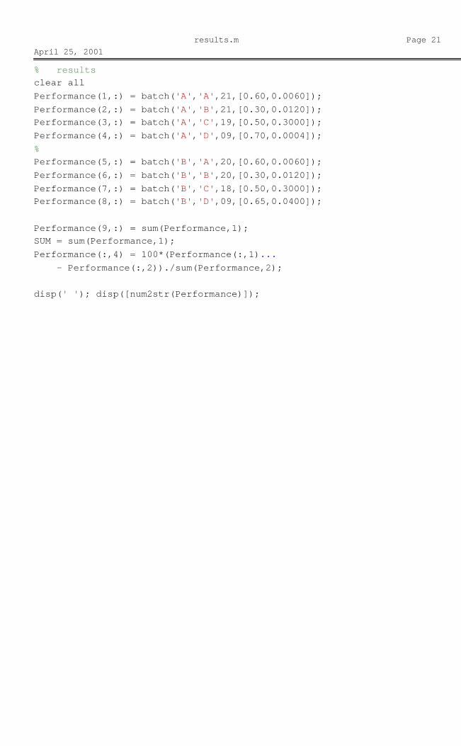
results.mApril 25, 2001
Page 219:28:50 PM
% resultsclear allPerformance(1,:) = batch('A','A',21,[0.60,0.0060]);Performance(2,:) = batch('A','B',21,[0.30,0.0120]);Performance(3,:) = batch('A','C',19,[0.50,0.3000]);Performance(4,:) = batch('A','D',09,[0.70,0.0004]);%Performance(5,:) = batch('B','A',20,[0.60,0.0060]);Performance(6,:) = batch('B','B',20,[0.30,0.0120]);Performance(7,:) = batch('B','C',18,[0.50,0.3000]);Performance(8,:) = batch('B','D',09,[0.65,0.0400]);
Performance(9,:) = sum(Performance,1);SUM = sum(Performance,1);Performance(:,4) = 100*(Performance(:,1)... - Performance(:,2))./sum(Performance,2);
disp(' '); disp([num2str(Performance)]);
5.3. Sample program menus
Recording function page 1
Training function page 2
Testing function page 3

4/25/2001 ECE566 Philip Felber 1
RECORDING FUNCTION
4/25/2001 ECE566 Philip Felber 2
TRAINING FUNCTION

4/25/2001 ECE566 Philip Felber 3
TESTING FUNCTION
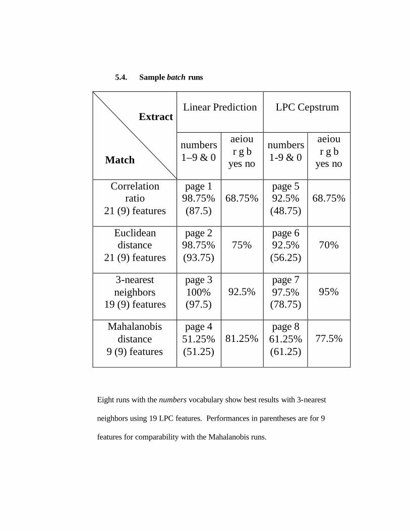
5.4. Sample batch runs
Linear Prediction LPC Cepstrum
Extract
Match numbers 1–9 & 0
aeiou r g b
yes no
numbers 1-9 & 0
aeiou r g b
yes no
Correlation ratio
21 (9) features
page 1 98.75% (87.5)
68.75% page 5 92.5% (48.75)
68.75%
Euclidean distance
21 (9) features
page 2 98.75% (93.75)
75% page 6 92.5% (56.25)
70%
3-nearest neighbors
19 (9) features
page 3 100% (97.5)
92.5% page 7 97.5% (78.75)
95%
Mahalanobis distance
9 (9) features
page 4 51.25% (51.25)
81.25% page 8
61.25% (61.25)
77.5%
Eight runs with the numbers vocabulary show best results with 3-nearest
neighbors using 19 LPC features. Performances in parentheses are for 9
features for comparability with the Mahalanobis runs.

MATLAB Command WindowApril 25, 2001
Page 19:47:52 PM
A A 21 0.6 0.006 19-Apr-2001 Vocabulary: numbers 'Male Training A'
'Male Training B'
'Male Training C'
'Male Training D'
'Female Training A'
'Female Training B'
'Female Training C'
'Female Training D'
Training count: 8 Right, Wrong, Don't know 'Male Testing A' '10 0 0'
'Male Testing B' '10 0 0'
'Male Testing C' '10 0 0'
'Male Testing D' '10 0 0'
'Female Testing A' '10 0 0'
'Female Testing B' '10 0 0'
'Female Testing C' '9 0 1'
'Female Testing D' '10 0 0'
Sum = 79 0 1 Performance (right's - wrong's) = 98.75 Version: 4 4 0 3 3 3 Sample Rate: 8000 Feature Count: 21 Threshold: 0.6 0.006 Algorithms - 'extract' 'A' 'Linear Prediction' 'match' 'A' 'Correlation ratio'
MATLAB Command WindowApril 25, 2001
Page 29:47:52 PM
A B 21 0.3 0.012 19-Apr-2001 Vocabulary: numbers 'Male Training A'
'Male Training B'
'Male Training C'
'Male Training D'
'Female Training A'
'Female Training B'
'Female Training C'
'Female Training D'
Training count: 8 Right, Wrong, Don't know 'Male Testing A' '10 0 0'
'Male Testing B' '10 0 0'
'Male Testing C' '10 0 0'
'Male Testing D' '10 0 0'
'Female Testing A' '10 0 0'
'Female Testing B' '10 0 0'
'Female Testing C' '9 0 1'
'Female Testing D' '10 0 0'
Sum = 79 0 1 Performance (right's - wrong's) = 98.75 Version: 4 4 0 3 3 3 Sample Rate: 8000 Feature Count: 21 Threshold: 0.3 0.012 Algorithms - 'extract' 'A' 'Linear Prediction' 'match' 'B' 'Euclidean distance'

MATLAB Command WindowApril 25, 2001
Page 39:47:52 PM
A C 19 0.5 0.3 19-Apr-2001 Vocabulary: numbers 'Male Training A'
'Male Training B'
'Male Training C'
'Male Training D'
'Female Training A'
'Female Training B'
'Female Training C'
'Female Training D'
Training count: 8 Right, Wrong, Don't know 'Male Testing A' '10 0 0'
'Male Testing B' '10 0 0'
'Male Testing C' '10 0 0'
'Male Testing D' '10 0 0'
'Female Testing A' '10 0 0'
'Female Testing B' '10 0 0'
'Female Testing C' '10 0 0'
'Female Testing D' '10 0 0'
Sum = 80 0 0 Performance (right's - wrong's) = 100 Version: 4 4 0 3 3 3 Sample Rate: 8000 Feature Count: 19 Threshold: 0.5 0.3 Algorithms - 'extract' 'A' 'Linear Prediction' 'match' 'C' '3 nearest neighbors'
MATLAB Command WindowApril 25, 2001
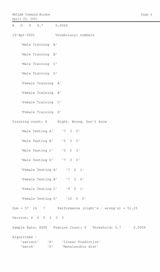
Page 49:47:52 PM
A D 9 0.7 0.0004 19-Apr-2001 Vocabulary: numbers 'Male Training A'
'Male Training B'
'Male Training C'
'Male Training D'
'Female Training A'
'Female Training B'
'Female Training C'
'Female Training D'
Training count: 8 Right, Wrong, Don't know 'Male Testing A' '7 3 0'
'Male Testing B' '5 3 2'
'Male Testing C' '5 2 3'
'Male Testing D' '7 3 0'
'Female Testing A' '7 2 1'
'Female Testing B' '7 3 0'
'Female Testing C' '9 0 1'
'Female Testing D' '10 0 0'
Sum = 57 16 7 Performance (right's - wrong's) = 51.25 Version: 4 4 0 3 3 3 Sample Rate: 8000 Feature Count: 9 Threshold: 0.7 0.0004 Algorithms - 'extract' 'A' 'Linear Prediction' 'match' 'D' 'Mahalanobis dist'
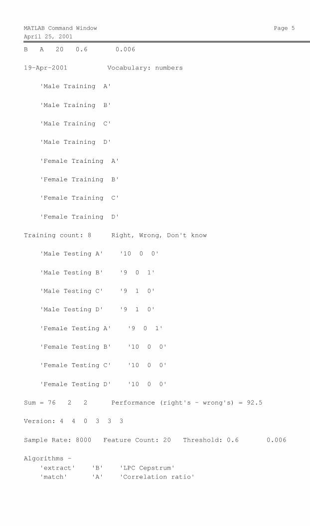
MATLAB Command WindowApril 25, 2001
Page 59:47:52 PM
B A 20 0.6 0.006 19-Apr-2001 Vocabulary: numbers 'Male Training A'
'Male Training B'
'Male Training C'
'Male Training D'
'Female Training A'
'Female Training B'
'Female Training C'
'Female Training D'
Training count: 8 Right, Wrong, Don't know 'Male Testing A' '10 0 0'
'Male Testing B' '9 0 1'
'Male Testing C' '9 1 0'
'Male Testing D' '9 1 0'
'Female Testing A' '9 0 1'
'Female Testing B' '10 0 0'
'Female Testing C' '10 0 0'
'Female Testing D' '10 0 0'
Sum = 76 2 2 Performance (right's - wrong's) = 92.5 Version: 4 4 0 3 3 3 Sample Rate: 8000 Feature Count: 20 Threshold: 0.6 0.006 Algorithms - 'extract' 'B' 'LPC Cepstrum' 'match' 'A' 'Correlation ratio'

MATLAB Command WindowApril 25, 2001
Page 69:47:52 PM
B B 20 0.3 0.012 19-Apr-2001 Vocabulary: numbers 'Male Training A'
'Male Training B'
'Male Training C'
'Male Training D'
'Female Training A'
'Female Training B'
'Female Training C'
'Female Training D'
Training count: 8 Right, Wrong, Don't know 'Male Testing A' '9 1 0'
'Male Testing B' '9 0 1'
'Male Testing C' '10 0 0'
'Male Testing D' '9 1 0'
'Female Testing A' '9 0 1'
'Female Testing B' '10 0 0'
'Female Testing C' '10 0 0'
'Female Testing D' '10 0 0'
Sum = 76 2 2 Performance (right's - wrong's) = 92.5 Version: 4 4 0 3 3 3 Sample Rate: 8000 Feature Count: 20 Threshold: 0.3 0.012 Algorithms - 'extract' 'B' 'LPC Cepstrum' 'match' 'B' 'Euclidean distance'
MATLAB Command WindowApril 25, 2001
Page 79:47:52 PM
B C 18 0.5 0.3 19-Apr-2001 Vocabulary: numbers 'Male Training A'
'Male Training B'
'Male Training C'
'Male Training D'
'Female Training A'
'Female Training B'
'Female Training C'
'Female Training D'
Training count: 8 Right, Wrong, Don't know 'Male Testing A' '10 0 0'
'Male Testing B' '10 0 0'
'Male Testing C' '9 1 0'
'Male Testing D' '10 0 0'
'Female Testing A' '10 0 0'
'Female Testing B' '10 0 0'
'Female Testing C' '10 0 0'
'Female Testing D' '10 0 0'
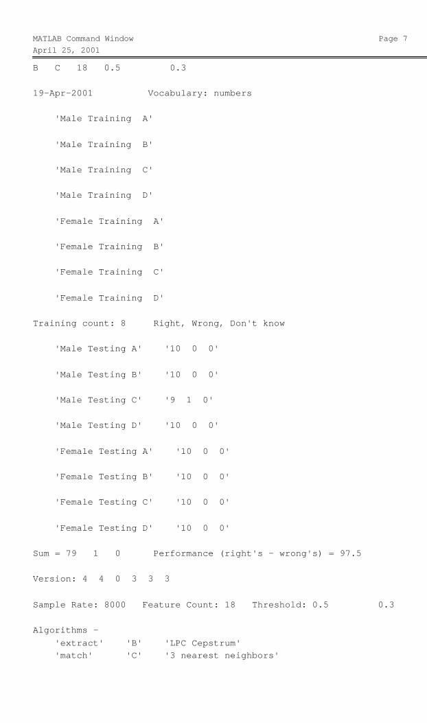
Sum = 79 1 0 Performance (right's - wrong's) = 97.5 Version: 4 4 0 3 3 3 Sample Rate: 8000 Feature Count: 18 Threshold: 0.5 0.3 Algorithms - 'extract' 'B' 'LPC Cepstrum' 'match' 'C' '3 nearest neighbors'

MATLAB Command WindowApril 25, 2001
Page 89:47:52 PM
B D 9 0.65 0.04 19-Apr-2001 Vocabulary: numbers 'Male Training A'
'Male Training B'
'Male Training C'
'Male Training D'
'Female Training A'
'Female Training B'
'Female Training C'
'Female Training D'
Training count: 8 Right, Wrong, Don't know 'Male Testing A' '6 3 1'
'Male Testing B' '7 3 0'
'Male Testing C' '8 2 0'
'Male Testing D' '8 1 1'
'Female Testing A' '8 2 0'
'Female Testing B' '9 0 1'
'Female Testing C' '8 2 0'
'Female Testing D' '9 1 0'
Sum = 63 14 3 Performance (right's - wrong's) = 61.25 Version: 4 4 0 3 3 3 Sample Rate: 8000 Feature Count: 9 Threshold: 0.65 0.04 Algorithms - 'extract' 'B' 'LPC Cepstrum' 'match' 'D' 'Mahalanobis dist'

5.5. Sample data plots
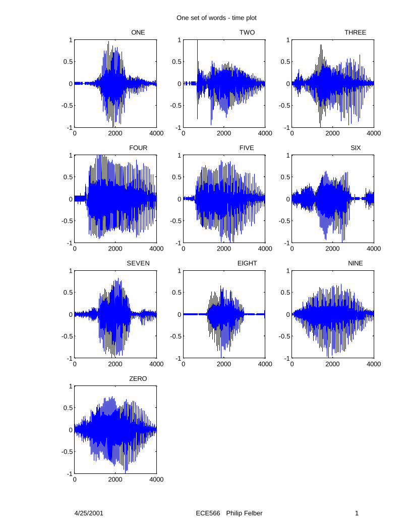
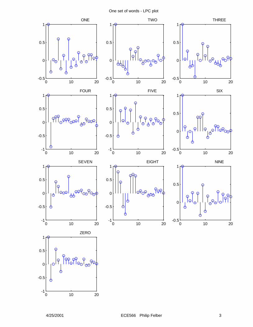
The following pages are sample plots taken from the numbers training data.
The plots on page 1 are time vs. signal amplitude (standardized in both time
and amplitude) for the ten vocabulary words from set: Male Training A. Plot 2
is the same data presented as spectrograms.
The remaining plots were made by extracting linear prediction coefficients
(LPC) from the same data. Note: the first coefficient is always one. Plot 3 is a
stem-plot of the first twenty coefficients from the LPC analysis. Plot 4 is a
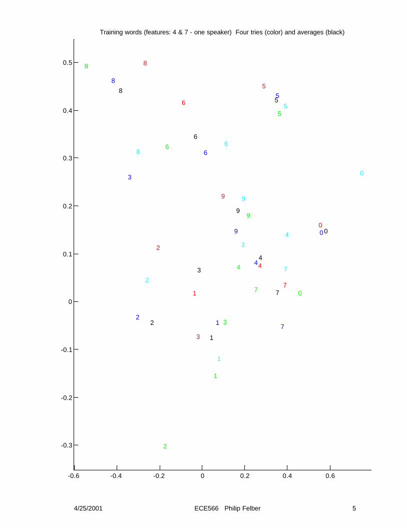
stem of the corresponding LPC-cepstrum data. Plot 5 is a two-dimensional
representation of the fourth vs. the seventh LPC feature (labeled 0-9) spoken
four times by the same male speaker. Each of the four runs is printed in its
own color. The averages (for each word) are printed in black. Plot 6 is similar
to plot 5, but in this case I show data for two speakers. The male speaker is
shown in red while the female is in green, and each vocabulary word is
presented in its own sub-plot.
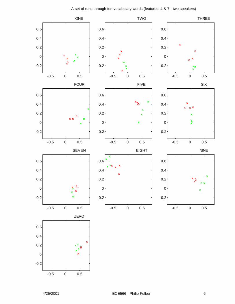
Remember that these charts show only two features where my actual
experiments used a large number (typically twenty). From this limited (two
feature) presentation we can see some clustering of the feature vectors. Also
we see some (speaker) divergence (for some words) in the two-speaker case.
0 2000 4000-1
-0.5
0
0.5
1 ONE
0 2000 4000-1
-0.5
0
0.5
1 TWO
0 2000 4000-1
-0.5
0
0.5
1 THREE
0 2000 4000-1
-0.5
0
0.5
1 FOUR
0 2000 4000-1
-0.5
0
0.5
1 FIVE
0 2000 4000-1
-0.5
0
0.5
1 SIX
0 2000 4000-1
-0.5
0
0.5
1 SEVEN
0 2000 4000-1
-0.5
0
0.5
1 EIGHT
0 2000 4000-1
-0.5
0
0.5
1 NINE
0 2000 4000-1
-0.5
0
0.5
1 ZERO
One set of words - time plot
4/25/2001 ECE566 Philip Felber 1

Time
Fre
quen
cy
ONE
0 0.2 0.40
1000
2000
3000
4000
Time
Fre
quen
cy
TWO
0 0.2 0.40
1000
2000
3000
4000
Time
Fre
quen
cy
THREE
0 0.2 0.40
1000
2000
3000
4000
Time
Fre
quen
cy
FOUR
0 0.2 0.40
1000
2000
3000
4000
Time
Fre
quen
cy
FIVE
0 0.2 0.40
1000
2000
3000
4000
Time
Fre
quen
cy
SIX
0 0.2 0.40
1000
2000
3000
4000
Time
Fre
quen
cy
SEVEN
0 0.2 0.40
1000
2000
3000
4000
Time
Fre
quen
cy
EIGHT
0 0.2 0.40
1000
2000
3000
4000
Time
Fre
quen
cy NINE
0 0.2 0.40
1000
2000
3000
4000
Time
Fre
quen
cy
ZERO
One set of words - spectogram plot
4/25/2001 ECE566 Philip Felber 2
0 0.2 0.40
1000
2000
3000
4000
0 10 20-0.5
0
0.5
1 ONE
0 10 20-0.5
0
0.5
1 TWO
0 10 20-0.5
0
0.5
1 THREE
0 10 20-1
-0.5
0
0.5
1 FOUR
0 10 20-1
-0.5
0
0.5
1 FIVE
0 10 20-0.5
0
0.5
1 SIX
0 10 20-1
-0.5
0
0.5
1 SEVEN
0 10 20-1
-0.5
0
0.5
1 EIGHT
0 10 20-0.5
0
0.5
1 NINE
0 10 20-1
-0.5
0
0.5
1 ZERO
One set of words - LPC plot
4/25/2001 ECE566 Philip Felber 3

0 10 20-0.2
0
0.2
0.4
0.6 ONE
0 10 20-0.4
-0.2
0
0.2
0.4 TWO
0 10 20-0.4
-0.2
0
0.2
0.4 THREE
0 10 20-0.6
-0.4
-0.2
0
0.2 FOUR
0 10 20-0.4
-0.2
0
0.2
0.4 FIVE
0 10 20-0.2
-0.1
0
0.1
0.2
0.3 SIX
0 10 20-0.4
-0.2
0
0.2
0.4 SEVEN
0 10 20-0.4
-0.2
0
0.2
0.4
0.6 EIGHT
0 10 20-0.2
-0.1
0
0.1
0.2 NINE
0 10 20-0.4
-0.2
0
0.2
0.4 ZERO
One set of words - LPC cepstrum plot
4/25/2001 ECE566 Philip Felber 4
-0.6 -0.4 -0.2 0 0.2 0.4 0.6
-0.3
-0.2
-0.1
0
0.1
0.2
0.3
0.4
0.5
1
1
1
1
1
2
2
2
2
2
3
3
3
3
344
4
4
4
5
5
5
556
66
66
77
7
7
7
88
8
8
8
9
9
9
9
9
0
0
0
0
0
Training words (features: 4 & 7 - one speaker) Four tries (color) and averages (black)
4/25/2001 ECE566 Philip Felber 5
-0.5 0 0.5
-0.2
0
0.2
0.4
0.6
ONE
-0.5 0 0.5
-0.2
0
0.2
0.4
0.6
TWO
-0.5 0 0.5
-0.2
0
0.2
0.4
0.6
THREE
-0.5 0 0.5
-0.2
0
0.2
0.4
0.6
FOUR
-0.5 0 0.5
-0.2
0
0.2
0.4
0.6
FIVE
-0.5 0 0.5
-0.2
0
0.2
0.4
0.6
SIX
-0.5 0 0.5
-0.2
0
0.2
0.4
0.6
SEVEN
-0.5 0 0.5
-0.2
0
0.2
0.4
0.6
EIGHT
-0.5 0 0.5
-0.2
0
0.2
0.4
0.6
NINE
-0.5 0 0.5
-0.2
0
0.2
0.4
0.6
ZERO
A set of runs through ten vocabulary words (features: 4 & 7 - two speakers)
4/25/2001 ECE566 Philip Felber 6

5.6. Miniatures of presentation slides
The following PowerPoint slides (some two dozen) were developed for a
forty-five-minute, in class, presentation that includes a short demonstration.

Isolated Word Speech Recognition 1
4/25/2001 ECE566 Philip Felber 1
Speech RecognitionA report of an Isolated Word experiment.
By Philip FelberIllinois Institute of Technology
April 25, 2001Prepared for Dr. Henry StarkECE 566 Statistical Pattern Recognition
4/25/2001 ECE566 Philip Felber 2
Speech Recognition
Speech recognition and production are components of the larger subject of speech processing.Speech recognition is as old as the hills.Survey of speech recognition in general.Description of a simple isolated wordcomputer experiment programmed in MATLAB.

Isolated Word Speech Recognition 2
4/25/2001 ECE566 Philip Felber 3
Sounds of Spoken Language
Phonetic components (1877): Sweetn Voiced, unvoiced and plosiven Vowels and consonantsAcoustic wave patterns (1874): Belln Oscilloscope (amplitude vs. time)n Spectroscope (power vs. frequency)n Spectrogram (power vs. freq. vs. time)
Koenig, Dunn, and Lacey (1946).
4/25/2001 ECE566 Philip Felber 4
Vocabulary (numbers)with Phonetic Spellings
one W AH N six S IH K Stwo T UW seven S EH V AH Nthree TH R IY eight EY Tfour F AO R nine N AY Nfive F AY V zero Z IH R OW

Isolated Word Speech Recognition 3
4/25/2001 ECE566 Philip Felber 5
The Word “SIX”Oscillograph and Spectrogram
0 500 1000 1500 2000 2500 3000 3500 4000-1
-0.8
-0.6
-0.4
-0.2
0
0.2
0.4
0.6
0.8
1 SIX
TimeFr
eque
ncy
SIX
0 0.05 0.1 0.15 0.2 0.25 0.3 0.35 0.4 0.450
500
1000
1500
2000
2500
3000
3500
4000
4/25/2001 ECE566 Philip Felber 6
Contributions toAutomatic Speech Recognizers
Vocoder (1928): DudleyLinear Predictive Coding (1967): Atal, Schroeder, and HanaeurHidden Markov Models (1985): Rabiner, Juang, Levinson, and SondhiContinuous speech (199x): various using ANN and HMM
Isolated Word Speech Recognition 4
4/25/2001 ECE566 Philip Felber 7
Automatic Speech Recognizers
HAL 9000 from Kubrick’s film 2001: A Space OdysseyCommand / ControlSecurity – Access controlSpeech to textTranslation
4/25/2001 ECE566 Philip Felber 8
Survey of Speech to Text
IBM VoiceType – ViaVoiceDragon Systems DragonDictateKurzweil VoicePlus

Isolated Word Speech Recognition 5
4/25/2001 ECE566 Philip Felber 9
Speech Waveform Capture
Analog to digital conversionSound cardSampling rateSampling resolutionStandardized in amplitude and time
4/25/2001 ECE566 Philip Felber 10
Pre-processing
Analog to digital conversion.Speech has an overall spectral tilt of5 to 12 dB per octave.A pre-emphasis filter is normally used.
Normalize or standardize in loudness.Temporal alignment.

Isolated Word Speech Recognition 6
4/25/2001 ECE566 Philip Felber 11
Feature Extraction
Linear predictive coding (LPC)LPC-cepstrum
4/25/2001 ECE566 Philip Felber 12
The Word “SIX”LPC and LPC-Cepstrum
0 2 4 6 8 10 12 14 16 18 20-0.4
-0.2
0
0.2
0.4
0.6
0.8
1 SIX
0 2 4 6 8 10 12 14 16 18 20-0.2
-0.15
-0.1
-0.05
0
0.05
0.1
0.15
0.2
0.25 SIX

Isolated Word Speech Recognition 7
4/25/2001 ECE566 Philip Felber 13
Response of LPC Filterfor “FOUR” and “SIX”
Frequency (Hz)
0 500 1000 1500 2000 2500 3000 3500 4000-10
0
10
20
Frequency (Hz)
Mag
nitu
de (
dB)
Frequency (Hz)
0 500 1000 1500 2000 2500 3000 3500 4000-20
-10
0
10
20
Frequency (Hz)
Mag
nitu
de (
dB)
4/25/2001 ECE566 Philip Felber 14
Classification
Simple metricn distance to mean (parametric)n k-nearest neighbor (non-parametric)
Advanced recognizersn Hidden Markov models (HMM)n Artificial neural networks (ANN)
Isolated Word Speech Recognition 8
4/25/2001 ECE566 Philip Felber 15
Several small (10 words) vocabularies.Separate training and testing data.Linear predictive coding and cepstrum.A correlation ratio, Euclidian distance, k-nearest neighbor, and Mahalanobis.
An Isolated Word Experiment
4/25/2001 ECE566 Philip Felber 16
The Apparatus
ComputerWindows NTMATLAB (student or full version)Sound cardLoudspeakers and microphoneAbout a dozen MATLAB programs
Isolated Word Speech Recognition 9
4/25/2001 ECE566 Philip Felber 17
Program Structure
Array ofFeatureVectors
Training
Extracting
Testing
Matching
Extracting
Clasification
4/25/2001 ECE566 Philip Felber 18
Extractors
Linear predictive coding (LPC)n Coefficients of an all pole filter that
represents the formants.
LPC cepstrumn Coefficients of the Fourier transform of the
log magnitude of the spectrum.
Isolated Word Speech Recognition 10
4/25/2001 ECE566 Philip Felber 19
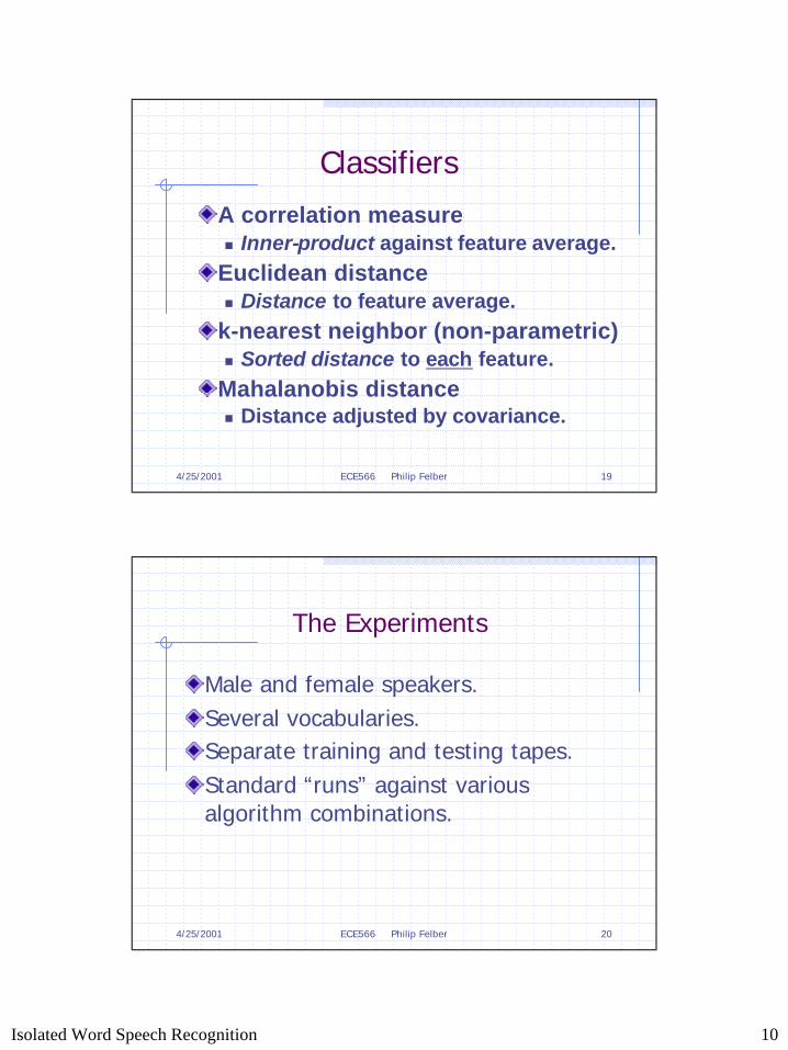
Classifiers
A correlation measuren Inner-product against feature average.
Euclidean distancen Distance to feature average.
k-nearest neighbor (non-parametric)n Sorted distance to each feature.
Mahalanobis distancen Distance adjusted by covariance.
4/25/2001 ECE566 Philip Felber 20
The Experiments
Male and female speakers.Several vocabularies.Separate training and testing tapes.Standard “runs” against various algorithm combinations.
Isolated Word Speech Recognition 11
4/25/2001 ECE566 Philip Felber 21
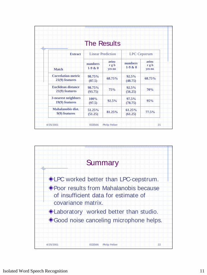
The ResultsExtract
Match
Linear Prediction LPC Cepstrum
numbers1-9 & 0
aeiour g b
yes no
numbers1-9 & 0
aeiour g b
yes no
Correlation metric21(9) features
98.75%(87.5)
68.75% 92.5%(48.75)
68.75%
Euclidean distance21(9) features
98.75%(93.75) 75% 92.5%
(56.25) 70%
3-nearest neighbors 19(9) features
100%(97.5) 92.5% 97.5%
(78.75) 95%
Mahalanobis dist.9(9) features
51.25%(51.25) 81.25% 61.25%
(61.25) 77.5%
4/25/2001 ECE566 Philip Felber 22
Summary
LPC worked better than LPC-cepstrum.Poor results from Mahalanobis because of insufficient data for estimate of covariance matrix.Laboratory worked better than studio.Good noise canceling microphone helps.

Isolated Word Speech Recognition 12
4/25/2001 ECE566 Philip Felber 23
Where To Get More Information
D. Jurafsky and James H. Martin, Speech and Language Processing: An Introduction to Natural Language Processing, Computational Linguistics, and Speech Recognition, Prentice-Hall, 2000.Search the ‘NET’ for speech recognition.
4/25/2001 ECE566 Philip Felber 24
Food for Thought
6. REFFERENCES
R. Duda and P. Hart, Pattern Classification and Scene Analysis, Wiley-Interscience, 1973.
S. Haykin, Neural Networks: A
Comprehensive Foundation, 2nd ed., Prentice-Hall, 1999.
D. Jurafsky and James H. Martin,
Speech and Language Processing: An Introduction to Natural Language Processing, Computational Linguistics, and Speech Recognition, Prentice-Hall, 2000.
H. Stark and J. Woods, Probability, Random Processes, and Estimation Theory for Engineers, 2nd ed., Prentice-Hall, 1994.
J. Y. Stein, Digital Signal
Processing: A Computer Science Perspective, Wiley-Interscience, 2000.