isma2012_0520

Identification and verification of structural nonlinearities based on vibration tests

G.B. Zhang, C. Zang

College of Energy and Power Engineering, Nanjing University of Aeronautics and Astronautics

Nanjing, 210016, China

e-mail: [email protected]

Abstract Practical engineering structures often exhibit nonlinear dynamic behaviour. It is essential to construct an

accurate nonlinear model from measured vibration data in order to predict the nonlinear dynamic

characteristics and response of these structures. This paper develops a novel technique to identify

structural nonlinearity and verify the nonlinear model. The method consists of two dynamic tests which

are constant-amplitude displacement test and constant-amplitude velocity test. Both tests use special

sinusoidal force excitations. The constant-amplitude displacement test is used to measure the nonlinear

stiffness behaviour and identify nonlinear stiffness terms from measured FRFs of the structure subjected to

sinusoidal force excitations which need to ensure the amplitudes of displacement is constant through

adjusting the amplitude of the force over the frequency range. The constant-amplitude velocity test is

similar to the constant-amplitude displacement and used to measure the nonlinear damping behaviour and

identify nonlinear damping terms. The identified nonlinear stiffness and damping terms are included into

the nonlinear model. The verification is done through comparison between predicted nonlinear behaviour

from the nonlinear model with measured nonlinear behaviour. This solution, taking advantage of modal

test and equivalent linearization theory, is direct and accurate. The solution is illustrated and verified

through a framed structure with bolted joints.

1 Introduction

In the dynamic model validation, high quality model can be obtained through establishing detailed finite

element model and further model updating using modal testing data. The updated model can be applied to

predict and analyze the dynamic response of the structure sufficiently and accurately within the interested

frequency range. Generally, most validation methods are based on linear system. The structural

nonlinearities, due to the difficulty to obtain accurate nonlinear parameters in the measurement, are often

ignored completely or considered as uncertain factors to deal with [1-4]. Worden [5] and Kershen [6]

comprehensively discussed nonlinear detection, localization and identification in structural dynamics, but

there still exist difficulties in nonlinear parameter identification suitable for engineering application with

standard vibration test because of the advantages and disadvantages of each method. Recently, sinusoidal

excitation and modal analysis techniques [7-9] have been developed for the nonlinear identification. The

method, based on the equivalent linearization theory [5], is expected to be applied widely in industry

because of its mathematical simplicity and relatively mature technique.

Most recently, Zang, Schwingshackl & Ewins [10] put forward an effective linearity method to deal with

the existed nonlinearity in an approach to the Sandia Structural Dynamics Challenge for model validation

of structural dynamic analysis. They[11] also investigated the influence of nonlinearity on uncertainty and

variability for dynamic models. Based on simulation of three degrees of freedom vibration system with a

weakly nonlinearity, two dynamic tests, namely constant-amplitude displacement test and constant-

amplitude velocity test, are exploited to identify the nonlinear stiffness and damping behaviour

respectively under the sinusoidal force excitations.

2611

This paper will focus on the nonlinearity identification with practical modal test. A framed structure with

bolted joints is used as an example. The constant-amplitude displacement test is used to measure the

nonlinear stiffness behaviour and identify nonlinear stiffness terms from measured FRFs of the structure

subjected to sinusoidal force excitations which need to ensure the amplitudes of displacement is constant

through adjusting the amplitude of the force over the frequency range. Similarly, the nonlinear damping

features and term can be identified through the constant-amplitude velocity test. The verification is

undertaken through comparison between the predicted nonlinear behaviour from the nonlinear model with

the measurement. The results show the effectiveness of the proposed method.

2 Identification of structural nonlinearity

2.1 Equivalent linearization of structural nonlinearity

In the case of a SDOF nonlinear system where the nonlinearity is additively separable, the equation of

motion can be written as:

sind smx f x f x F t (1)

Where df x represents the weak nonlinearity of damping behavior and sf x represents the weakly

nonlinear stiffness feature. Based on equivalent linearization theory, its equivalent linearization is written

as:

sineq eqmx c x k x F t (2)

where eqc is the equivalent linear damping and

eqk is the equivalent linear stiffness. Then, the equivalent

linear FRF is described as:

2

1eq

eq eq

Hm j c k

(3)

Simply assuming that the response to a sinusoidal excitation is a sinusoid at the same frequency, the

displacement and velocity can be expressed as

sinx A t (4)

sin2

x A t

(5)

where A is the amplitude of displacement response at steady state.

The harmonic balance (HB) applied to the equation of motion yields the equivalent stiffness

2

0

1sin sin deq sk f A f A

A

(6)

and the equivalent damping

2

0

1sin cos d ( )eq dc f A g A

A

(7)

According to Eq. (6) and Eq. (7), the equivalent stiffness is the function of displacement amplitude and the

equivalent damping is the function of velocity amplitude, respectively. Therefore, if the amplitudes of

displacement are kept constant through adjusting the amplitude of the sinusoidal force over the interested

frequency range, the influence of the nonlinear stiffness on the measured FRF data can be minimised.

Such test is called as constant displacement test and can be used to measure the relationship between

equivalent stiffness and displacement amplitude. The nonlinear damping behaviour and terms can be also

2612 PROCEEDINGS OF ISMA2012-USD2012

obtained in the same way through acting on the constant velocity test to the structure. Afterwards, the

identified nonlinear properties can be included into the model to predict the response of nonlinear system.

2.2 Dynamic test methods

There are three dynamic test methods using the sinusoidal excitation with amplitude control: constant

force test, constant displacement test, and constant velocity test. The most widely used constant force test

needs to keep the sinusoidal excitation force amplitude constant at various interested frequency points

over the frequency range during the test. The constant displacement and constant velocity tests need to

adjust the amplitude of sinusoidal force in order to keep the displacement or velocity response amplitude

unchanged during the frequency range of excitation. The difficulty in conducting constant displacement

and constant velocity tests are how to determine the amplitude of sinusoidal excitation at each frequency

so that the response amplitudes at the steady state are maintained the same value. Generally, the feedback

control method is effective, but it is time-consuming. Here, a simple method is employed without

feedback control. As the relationship between the sinusoidal excitation and response amplitudes is affected

by nonlinearity at various frequencies, it is generally not linear but remains a monotonic increasing. This

may be true for many nonlinear structures. Therefore, the function can be measured at each interested

frequency, such as

( , ), 1,2,...iX f F i n (8)

1( , ), 1,2,...iF f X i n (9)

So, the response amplitude can be only determined by a given excitation amplitude for a frequency in zero

initial conditions

0( ), , 1,2,...ix f F Freq f i n (10)

If this function has been gained from test data, the excitation amplitude can be only determined by a given

response amplitude

1

0 ( ), , 1,2,...iF f x Freq f i n (11)

In practice, the function can be created by the piecewise spline interpolation polynomial, and will be

further verified in the subsequent experimental research.

Actually, the phase difference between excitation and response is, similar to the amplitude in the zero

initial conditions, a monotonic increasing or decreasing function. Therefore, the excitation amplitude and

phase difference between excitation and response can alternatively be determined by a given response

amplitude using the data from constant force test. Therefore, the FRFs can also be determined. As a result,

the constant-amplitude displacement and constant-amplitude velocity tests can be conducted virtually

from constant force excitation.

3 Experimental study of a framed structure with bolted joints

3.1 Experimental setup

In order to illustrate and verify the nonlinear parameters identification method, a series of tests has been

conducted in a framed structure with bolted joints shown in Figure 1. This structure was originally

intended to represent a 3DOF system and can represent a SDOF system after removing two mass

components. Four rubber rings are installed between the four aluminum beams and the base plate

respectively to enhance the nonlinear stiffness and damping behavior of the SDOF system.

NON-LINEARITIES: IDENTIFICATION AND MODELLING 2613

(a) SDOF system

(b) 3DOF system

Figure 1: Experimental setup

3.2 Nonlinearity detection using swept sine test

To detect the nonlinearity of the SDOF system, a series of swept sinusoidal excitation with various force

levels from 0.1N to 10N are exploited to the frame and the responses of acceleration are measured.

Obviously, the overlay of measured FRFs from Figure 2 shows the distortion characteristic of acceleration

FRFs. With the increase of excitation force levels, the resonant frequency shifts downwards to the

softening system. The zoomed changes in natural frequency and phase between 36Hz and 48Hz are

overlaid in Figure 3. The modal parameters extracted from FRFs using circle fit method from ICATS

software are shown in Figure 4.

20 30 40 50 60 70-100

-80

-60

-40

-20

0

20

Frequency / Hz

Am

plit

ude / g

/N,d

B

0.1N

0.5N

1N

3N

5N

7N

10N

Figure 2: The acceleration FRFs at different force levels

36 38 40 42 44 46 48-50

-40

-30

-20

-10

0

10

Frequency / Hz

Am

plit

ude / g/N

,dB

0.1N

0.5N

1N

3N

5N

7N

10N

36 38 40 42 44 46 480

50

100

150

200

Frequency / Hz

Phase / d

eg

0.1N

0.5N

1N

3N

5N

7N

10N

Figure 3: The acceleration FRFs at different force levels between 36Hz and 48Hz


0 2 4 6 8 1042

42.5

43

43.5

44

44.5

45

Amplitude / N

Natu

ral fr

equency / H

z

0 2 4 6 8 10

1.8

2

2.2

2.4

2.6

2.8

3

3.2

Amplitude / N

Vis

cous d

am

pin

g r

atio

/ %

Figure 4: The modal parameters at different force levels of excitation

It can be seen that the natural frequency shifts from 44.8Hz to 42.4Hz and the viscous damping ratio shifts

from 1.8% to 5.6% respectively, while the excitation force is raised from 0.1N to 10N. Strictly speaking, it

is not suitable to estimate the modal parameters for nonlinear system directly using traditional modal

analysis method such as the circle fit method. The fitting error will be produced because of the Nyquist

plot distortion as shown in Figure 5. Therefore, it is difficult to identify nonlinear parameters accurately

using the swept sine test directly.

(a) 10N

(b) 0.1N

Figure 5: Circle fit at different force levels of excitation

3.3 Constant force test

The parameter setting of the sinusoidal excitation used to conduct constant force test is shown in Table 1.

The accelerance FRFs obtained from constant force test and their amplitudes and phases against frequency

are plotted and shown in Figure 6 and Figure 7. The relationship of both amplitude acceleration and phase

against the force respectively at different frequencies is plotted in Figure 8. A monotonic increasing

function between amplitude and force can be seen clearly while the phase shows the decreasing function

instead.

Frequency span Frequency interval Force levels Sampling Freq Sampling time

40 Hz~47Hz 0.25Hz 0.5,1,2,3,4,5,7,9N 5120Hz 1.6s

Table 1: The parameter setting for constant force test


Figure 6: The 3D plot of amplitude of accelerance FRFs

Figure 7: The 3D plot of phase of accelerance FRFs

1 2 3 4 5 6 7 8 9

1

2

3

4

5

6

7

Force / N

Accele

ration / g

40 Hz

41 Hz

42 Hz

43 Hz

44 Hz

45 Hz

46 Hz

47 Hz

1 2 3 4 5 6 7 8 9

20

40

60

80

100

120

140

160

Force / N

Phase / d

eg

40 Hz

41 Hz

42 Hz

43 Hz

44 Hz

45 Hz

46 Hz

47 Hz

Figure 8: The amplitude and phase of acceleration against excitation levels at different frequencies


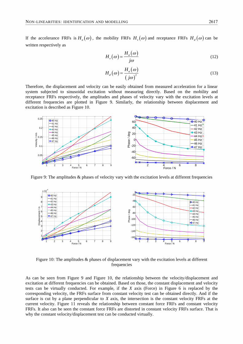
If the accelerance FRFs is aH , the mobility FRFs vH and receptance FRFs dH can be

written respectively as

a

v

HH

j

(12)

2

a

d

HH

j

(13)

Therefore, the displacement and velocity can be easily obtained from measured acceleration for a linear

system subjected to sinusoidal excitation without measuring directly. Based on the mobility and

receptance FRFs respectively, the amplitudes and phases of velocity vary with the excitation levels at

different frequencies are plotted in Figure 9. Similarly, the relationship between displacement and

excitation is described as Figure 10.

1 2 3 4 5 6 7 8 9

0.05

0.1

0.15

0.2

0.25

Force / N

Velo

city / m

/s

40 Hz

41 Hz

42 Hz

43 Hz

44 Hz

45 Hz

46 Hz

47 Hz

2 4 6 8

-60

-40

-20

0

20

40

60

Force / N

Phase / d

eg

40 Hz

41 Hz

42 Hz

43 Hz

44 Hz

45 Hz

46 Hz

47 Hz

Figure 9: The amplitudes & phases of velocity vary with the excitation levels at different frequencies

1 2 3 4 5 6 7 8 9

1

2

3

4

5

6

7

8

9

x 10-4

Force / N

Dis

pla

cem

ent / m

40 Hz

41 Hz

42 Hz

43 Hz

44 Hz

45 Hz

46 Hz

47 Hz

1 2 3 4 5 6 7 8 9

-160

-140

-120

-100

-80

-60

-40

-20

Force / N

Phase / d

eg

40 Hz

41 Hz

42 Hz

43 Hz

44 Hz

45 Hz

46 Hz

47 Hz

Figure 10: The amplitudes & phases of displacement vary with the excitation levels at different

frequencies

As can be seen from Figure 9 and Figure 10, the relationship between the velocity/displacement and

excitation at different frequencies can be obtained. Based on those, the constant displacement and velocity

tests can be virtually conducted. For example, if the X axis (Force) in Figure 6 is replaced by the

corresponding velocity, the FRFs surface from constant velocity test can be obtained directly. And if the

surface is cut by a plane perpendicular to X axis, the intersection is the constant velocity FRFs at the

current velocity. Figure 11 reveals the relationship between constant force FRFs and constant velocity

FRFs. It also can be seen the constant force FRFs are distorted in constant velocity FRFs surface. That is

why the constant velocity/displacement test can be conducted virtually.


Figure 11: Constant force FRFs and constant velocity FRFs

3.4 Nonlinearity identification

3.4.1 Nonlinear stiffness identification

The FRFs of the constant displacement tests under the different excitation levels are shown in Figure 12.

Suppose the equivalent stiffness is

m

eqk a b x (14)

40 41 42 43 44 45 46 47

-90

-88

-86

-84

-82

-80

-78

Frequency / Hz

Am

plit

ude / d

B,m

/N

D1

D2

D3

D4

D5

D6

D7

D8

D9

D10

(a) Amplitude

40 41 42 43 44 45 46 47

-160

-140

-120

-100

-80

-60

-40

-20

Frequency / Hz

Phase / d

eg

D1

D2

D3

D4

D5

D6

D7

D8

D9

D10

(b) Phase

Figure 12: Constant displacement FRFs with different excitations

The parameters a, b, and the index m can be identified by the least squire curve fitting method using the

data from Table 2 obtained through modal analysis. The fitting results are shown in Table 3.


No. Displacement

[10-3

m]

Equivalent Stiffness

[104m/N]

Natural Frequency

[Hz]

D1 0.0719 8.9595 43.9857

D2 0.1211 8.8508 43.7182

D3 0.1703 8.7613 43.4967

D4 0.2195 8.6883 43.3150

D5 0.2688 8.6272 43.1624

D6 0.3180 8.5749 43.0314

D7 0.3672 8.5272 42.9117

D8 0.4164 8.4831 42.8005

D9 0.4656 8.4440 42.7017

D10 0.5149 8.4106 42.6173

Table 2: Constant displacement test results

a b m

9.2719×104

-3.8641×105 1/2

Table 3: Curve fitting results

The curve fitting and the test of both natural frequencies and the equivalent stiffness against the

displacement amplitude respectively is plotted in Figure 13.

0 0.2 0.4 0.6 0.8 1

x 10-3

42

42.5

43

43.5

44

44.5

Displacement / m

Natu

ral fr

equency / H

z

Test

Fit

0 0.2 0.4 0.6 0.8 1

x 10-3

8.2

8.4

8.6

8.8

9

9.2

x 104

Displacement / m

Equiv

ale

nt stiffness / N

/m

Test

Fit

Figure 13: Curve fitting and the test of both natural frequencies and the equivalent stiffness against the

displacement amplitude

3.4.2 Nonlinear damping identification

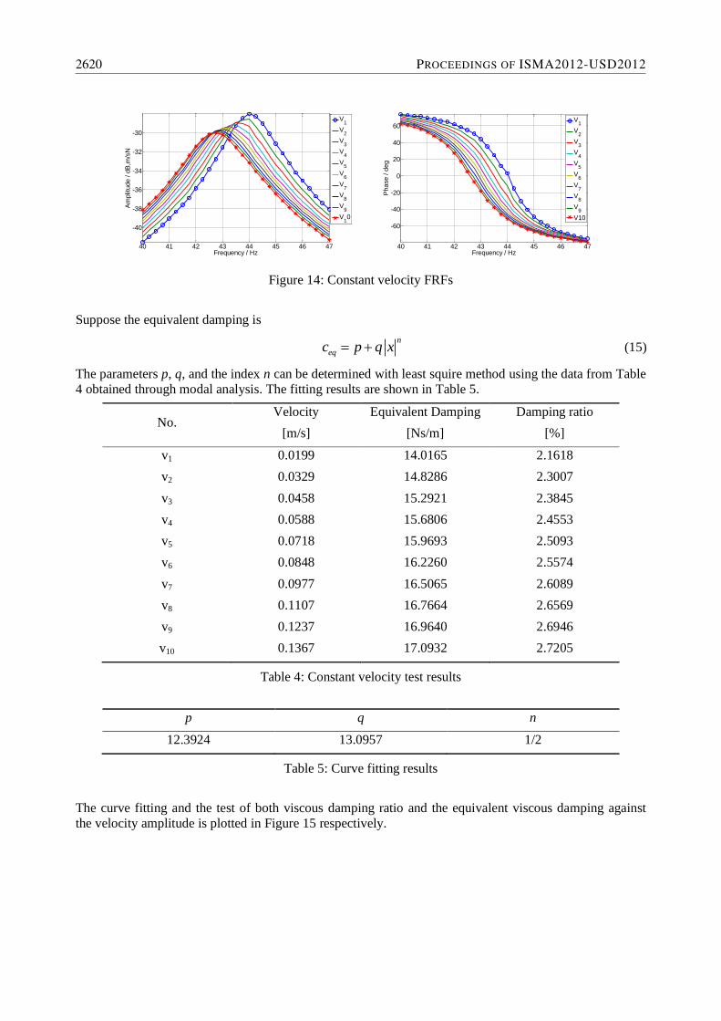
Similar to the nonlinear stiffness identification, the amplitude and phase characteristics of Constant

velocity FRFs within the frequency range from 40 to 47Hz is plotted in Figure 14.


40 41 42 43 44 45 46 47

-40

-38

-36

-34

-32

-30

Frequency / Hz

Am

plit

ude / d

B,m

/sN

V1

V2

V3

V4

V5

V6

V7

V8

V9

V10

40 41 42 43 44 45 46 47

-60

-40

-20

0

20

40

60

Frequency / Hz

Phase / d

eg

V1

V2

V3

V4

V5

V6

V7

V8

V9

V10

Figure 14: Constant velocity FRFs

Suppose the equivalent damping is

n

eqc p q x (15)

The parameters p, q, and the index n can be determined with least squire method using the data from Table

4 obtained through modal analysis. The fitting results are shown in Table 5.

No. Velocity

[m/s]

Equivalent Damping

[Ns/m]

Damping ratio

[%]

v1 0.0199 14.0165 2.1618

v2 0.0329 14.8286 2.3007

v3 0.0458 15.2921 2.3845

v4 0.0588 15.6806 2.4553

v5 0.0718 15.9693 2.5093

v6 0.0848 16.2260 2.5574

v7 0.0977 16.5065 2.6089

v8 0.1107 16.7664 2.6569

v9 0.1237 16.9640 2.6946

v10 0.1367 17.0932 2.7205

Table 4: Constant velocity test results

p q n

12.3924

13.0957 1/2

Table 5: Curve fitting results

The curve fitting and the test of both viscous damping ratio and the equivalent viscous damping against

the velocity amplitude is plotted in Figure 15 respectively.


0 0.05 0.1 0.15 0.2 0.25

2

2.2

2.4

2.6

2.8

3

Velocity / m/s

Vis

cous d

am

pin

g r

atio / %

Test

Fit

0 0.05 0.1 0.15 0.2 0.25

13

14

15

16

17

18

19

Velocity / m/s

Equiv

ale

nt vis

cous d

am

pin

g / N

s/m

Test

Fit

Figure 15: Curve fitting and the test of both the viscous damping ratio and the equivalent viscous damping

against the velocity amplitude

3.5 Verification of nonlinearity identification

Based on the nonlinearity identification of stiffness and damping property, the equation of motion of the

bolted frame can be written as

1 1

2 20 0 sinn nmx c x c x x k x k x x F t (16)

where the equivalent stiffness and damping are described as

1

20 0.9153eq nk k k x (17)

1

20 0.9153eq nc c c x (18)

Then, the stiffness and damping terms are

0

0

/ 0.9153

/ 0.9153

n

n

k a

k b

c p

c q

(19)

The results of parameter identification are shown in Table 6.

m ( kg ) 0k ( N/m ) nk ( N/m1.5

) 0c ( Ns/m ) nc ( Ns1.5

/m1.5

)

1.1730 9.2719×104 -4.2216×10

5 12.3924 14.3074

Table 6: The results of parameter Identification

In order to verify the identified nonlinear model, the comparison of acceleration responses under the

different excitation force levels is undertaken between the prediction of the nonlinear model and measured

nonlinear behaviour. The overlay of the responses is plotted in Figure 16. Obviously, the predicted

responses are closely matched with the measured responses. The amplitudes and phases characteristics of

FRFs are calculated from the prediction model and compared with the experimental measurement. The

overlay of the predicted and measured FRFs under the different excitation force levels are plotted in

Figure 17. It clearly shows that very good agreements between them are obtained. A slight difference in

the resonance zone may be due to the measurement error of excitation in the experimental test. Thus, the

identified nonlinear model can represent the actual nonlinear behaviour of the structure.


40 41 42 43 44 45 46 47

1

2

3

4

5

Frequency /Hz

Acc

eler

atio

n /g

Test - 0.5N

Test - 3N

Test - 7N

Prediction - 0.5N

Prediction - 3N

Prediction - 7N

Figure 16: The overlay of acceleration responses between the model prediction and the measurement

40 41 42 43 44 45 46 47-14

-12

-10

-8

-6

-4

-2

0

Frequency /Hz

Am

plit

ude /dB

,g/N

Test - 0.5N

Test - 3N

Test - 7N

Prediction - 0.5N

Prediction - 3N

Prediction - 7N

40 41 42 43 44 45 46 47

20

40

60

80

100

120

140

160

Frequency /Hz

Phase /deg

Test - 0.5N

Test - 3N

Test - 7N

Prediction - 0.5N

Prediction - 3N

Prediction - 7N

Figure 17: The overlay of acceleration FRFs between the model prediction and the measurement

4 Conclusions

Nonlinearities are very common in real structures. In most cases, the functional types of nonlinearities are

unknown; therefore it becomes crucial to decide the nonlinear functional forms. The constant

displacement test and the constant velocity test under the ssinusoidal force excitations can be used to

identify the nonlinear stiffness and the nonlinear damping behaviours respectively from measured FRFs of

the structure. Both methods are mainly based on equivalent linearization theory and only considered the

first harmonic in the nonlinear identification. The experimental research based on a SDOF system with a

weakly nonlinear system shows the satisfactory results. Future work will extend to a MDOF system and a

FEM model, for example, the bolted joint beam etc.

Acknowledgements

The financial support of the National Natural Science Foundation of China (Project No. 51175244) and

Research Fund for the Doctoral Program of Higher Education of China (Project No. 20093218110008) are

gratefully acknowledged. Zang also acknowledges the project sponsored by the Scientific Research

Foundation for the Returned Overseas Chinese Scholars, State Education Ministry and the Fundamental

Research Funds for the Central Universities of China (Project No. kfjj20110204).


References

[1] R.G. Ghanem, A. Doostan and J. Red-Horse, A probabilistic construction of model validation,

Computer Methods in Applied Mechanics and Engineering, Vol.197 No.29-32 (2008), pp. 2585-2595.

[2] T. Hasselman and G. Lloyd, A top-down approach to calibration, validation, uncertainty

quantification and predictive accuracy assessment, Computer Methods in Applied Mechanics and

Engineering, Vol.197 No.29-32 (2008), pp. 2596-2606.

[3] L.G. Horta, et al., NASA Langley's approach to the Sandia's structural dynamics challenge problem,

Computer Methods in Applied Mechanics and Engineering, Vol.197 No.29-32 (2008), pp. 2607-2620.

[4] J. McFarland and S. Mahadevan, Error and variability characterization in structural dynamics

modeling, Computer Methods in Applied Mechanics and Engineering, 2008. 197(29-32), pp. 2621-

2631.

[5] K. Worden and G.R. Tomlinson, Nonlinearity in structural dynamics: detection, identification, and

modeling, 2001: Taylor & Francis.

[6] G. Kerschen et al., Past, present and future of nonlinear system identification in structural dynamics,

Mechanical Systems and Signal Processing, Vol.20 No.3 (2006), pp. 505-592.

[7] O. Arslan, M. Aykan and H. N Ozguven, Parametric identification of structural nonlinearities from

measured frequency response data, Mechanical Systems and Signal Processing, Vol.25 No.4 (2011),

pp. 1112-1125.

[8] O. Arslan, M. Aykan and H. N Ozguven, Modal identification of non-linear structures and the use of

modal model in structural dynamic analysis, in: 26th International Modal Analysis Conference

IMAC, Orlando, USA, 2008, Paper no.95.

[9] A. Carrella and D.J. Ewins, Identifying and quantifying structural nonlinearities in engineering

applications from measured frequency response functions, Mechanical Systems and Signal

Processing, Vol.25 No.3 (2011), pp. 1011-1027.

[10] C. Zang, C.W. Schwingshackl and D.J. Ewins, Model validation for structural dynamic analysis: An

approach to the Sandia Structural Dynamics Challenge, Computer Methods in Applied Mechanics

and Engineering, Vol.197,No 29-32,(2008), pp. 2645-2659.

[11] C.W. Schwingshackl, C. Zang and D. J. Ewins. The influence of nonlinearity on uncertainty and

variability for dynamic models, Proceedings of the 1st International Conference on Uncertainty in

Structural Dynamics. Sheffield, UK, May 2007, pp. 311-319.


isma2012_0520

Documents

Transcript of isma2012_0520