ISLE Home Page

Improved Rooftop Detection in Aerial Images with MachineLearning

M.A. Maloof ([email protected])Department of Computer Science, Georgetown University, Washington, DC 20057, USA

P. Langley ([email protected])Institute for the Study of Learning and Expertise, 2164 Staunton Court, Palo Alto,CA 94306, USA

T.O. Binford ([email protected])Robotics Laboratory, Department of Computer Science, Stanford University, Stanford,CA 94305, USA

R. Nevatia ([email protected])Institute for Robotics and Intelligent Systems, School of Engineering, University of SouthernCalifornia, Los Angeles, CA 90089, USA

S. Sage ([email protected])Institute for the Study of Learning and Expertise, 2164 Staunton Court, Palo Alto,CA 94306, USA

Abstract. In this paper, we examine the use of machine learning to improve a rooftop de-tection process, one step in a vision system that recognizes buildings in overhead imagery.We review the problem of analyzing aerial images and describe an existing system that detectsbuildings in such images. We briefly detail four algorithms that we selected to improve rooftopdetection. The data sets were highly skewed and the cost of mistakes differed between theclasses, so we used ROC analysis to evaluate the methods under varying error costs. Wereport three experiments designed to illuminate facets of applying machine learning to theimage analysis task. One investigated learning with all available images to determine the bestperforming method. Another focused on within-image learning, in which we derived trainingand testing data from the same image. A final experiment addressed between-image learning,in which training and testing sets came from different images. Results suggest that usefulgeneralization occurred when training and testing on data derived from images differing inlocation and in aspect. They demonstrate that under most conditions, naive Bayes exceededthe accuracy of other methods and a handcrafted classifier, the solution currently used in thebuilding detection system.

Keywords: supervised learning, learning for computer vision, evaluation of algorithms, ap-plications of learning.

1. Introduction

The number of images available to image analysts is growing rapidly, andwill soon outpace their ability to process them. Computational aids will berequired to filter this flood of images and to focus the analyst’s attentionon interesting events, but current image understanding systems are not yet

© 2002 Kluwer Academic Publishers. Printed in the Netherlands.

mlj02.tex; 21/04/2002; 15:56; p.1

2 Maloof, Langley, Binford, Nevatia, and Sage

robust enough to support this process. Successful image understanding relieson knowledge, and despite theoretical progress, implemented vision systemsstill rely on heuristic methods and consequently remain fragile. Handcraftedknowledge about when and how to use particular vision operations can giveacceptable results on some images but not on others.

In this paper, we explore the use of machine learning as a means forimproving knowledge used in the vision process, and thus for producingmore robust software. Recent applications of machine learning in businessand industry (Langley & Simon, 1995) hold useful lessons for applications inimage analysis. A key idea in applied machine learning involves building anadvisory system that recommends actions but gives final control to a humanuser, with each decision generating a training case, gathered in an unobtrusiveway, for use in learning. This setting for knowledge acquisition is similar tothe scenario in which an image analyst interacts with a vision system, findingsome system analyses acceptable and others uninteresting or in error. The aimof our research program is to embed machine learning into this interactiveprocess of image analysis.

This adaptive approach to computer vision promises to greatly reduce thenumber of decisions that image analysts must make per picture, thus improv-ing their ability to deal with a high flow of images. Moreover, the resultingsystems should adapt their knowledge to the preferences of individuals inresponse to feedback from those users. The overall effect should be a newclass of systems for image analysis that reduces the workload on human an-alysts and gives them more reliable results, thus speeding the image analysisprocess.

In the sections that follow, we report progress on using machine learningto improve decision making at one stage in an existing image understandingsystem. We begin by explaining the task domain—identifying buildings inaerial photographs—and then describe the vision system designed for thistask. Next, we review four well-known algorithms for supervised learningthat hold potential for improving the reliability of image analysis in thisdomain. After this, we report the design of experiments to evaluate thesemethods and the results of those studies. In closing, we discuss related andfuture work.

2. Nature of the Image Analysis Task

Image analysts interpret aerial images of ground sites with an eye to unusualactivity or other interesting behavior. The images under scrutiny are usuallycomplex, involving many objects arranged in a variety of patterns. Over-head images of Fort Hood, Texas, collected as part of the RADIUS project(Firschein & Strat, 1997), are typical of a military base and include buildings

mlj02.tex; 21/04/2002; 15:56; p.2

Improved Rooftop Detection with Machine Learning 3

in a range of sizes and shapes, major and minor roadways, sidewalks, park-ing lots, vehicles, and vegetation. A common task analysts face is to detectchange at a site as reflected in differences between two images, as in thenumber of buildings, roads, and vehicles. This in turn requires the ability torecognize examples from each class of interest. In this paper, we focus on theperformance task of identifying buildings in satellite photographs.

Aerial images can vary across a number of dimensions. The most ob-vious factors concern viewing parameters, such as distance from the site(which affects size and resolution) and viewing angle (which affects perspec-tive and visible surfaces). But other variables also influence the nature ofthe image, including the time of day (which affects contrast and shadows),the time of year (which affects foliage), and the site itself (which deter-mines the shapes of viewed objects). Taken together, these factors introduceconsiderable variability into the images confronting analysts.

In turn, this variability can significantly complicate the task of recogniz-ing object classes. Although a building or vehicle will appear different fromalternative perspectives and distances, the effects of such transformations arereasonably well understood. But variations due to time of day, the season,and the site are more serious. Shadows and foliage can hide edges and obscuresurfaces, and buildings at distinct sites may have quite different structures andlayouts. Such variations serve as mere distractions to a human image analyst,yet they provide serious challenges to existing computer vision systems.

This suggests a natural task for machine learning: given aerial imagesas training data, acquire knowledge that improves the reliability of such animage analysis system. However, we cannot study this task in the abstract.We must explore the effect of specific induction algorithms on particularvision software. In the next two sections, we briefly review one such systemfor image analysis and four learning methods that might give it more robustbehavior.

3. An Architecture for Image Analysis

Lin and Nevatia (1998) reported a computer vision package, called the Build-ings Detection and Description System (BUDDS), for the analysis of groundsites in aerial images. Like many programs for image understanding, theirsystem operates in a series of processing stages. Each step involves aggregat-ing lower level features into higher level ones, eventually reaching hypothesesabout the locations and descriptions of buildings. We will consider thesestages in the order that they occur.

Starting at the pixel level, BUDDS uses an edge detector to group pixelsinto edge elements, and then invokes a linear feature detector to group edgeelements into lines. Junctions and parallel lines are identified and combined

mlj02.tex; 21/04/2002; 15:56; p.3


to form three-sided structures, or “U-constructs.” The algorithm then groupsselected U-constructs and junctions to form parallelograms. Each such par-allelogram constitutes a hypothesis about the position and orientation of theroof for some building, so we may call this step rooftop generation.

After the system has completed the above aggregation process, a rooftopselection stage evaluates each rooftop candidate to determine whether it hassufficient evidence to be retained. The aim of this process is to remove can-didates that do not correspond to actual buildings. Ideally, the system willreject most spurious candidates at this point, although a final verification stepmay still collapse duplicate or overlapping rooftops. This stage may also ex-clude candidates if there is no evidence of three-dimensional structure, suchas shadows and walls.

Analysis of the system’s operation suggested that rooftop selection heldthe most promise for improvement through machine learning, because thisstage must deal with many spurious rooftop candidates. This process takesinto account both local and global criteria. Local support comes from fea-tures such as lines and corners that are close to a given parallelogram. Sincethese suggest walls and shadows, they provide evidence that the candidatecorresponds to an actual building. Global criteria consider containment, over-lap, and duplication of candidates. Using these evaluation criteria, the setof rooftop candidates is reduced to a more manageable size. The individualconstraints applied in this process have a solid foundation in both theory andpractice.

The problem is that we have only heuristic knowledge about how to com-bine these constraints. Moreover, such rules of thumb are currently crafted byhand, and they do not fare well on images that vary in their global character-istics, such as contrast and amount of shadow. However, methods of machinelearning, to which we now turn, may be able to induce better conditionsfor selecting or rejecting candidate rooftops. If these acquired heuristics aremore accurate than the existing handcrafted solutions, they will improve thereliability of the rooftop selection process.

4. A Review of Four Learning Techniques

We can formulate the task of acquiring rooftop selection heuristics in termsof supervised learning. In this process, training cases of some concept arelabeled as to their class. In rooftop selection, only two classes exist—rooftopand non-rooftop—which we will refer to as positive and negative examplesof the concept “rooftop.” Each instance consists of a number of attributesand their associated values, along with a class label. These labeled instancesconstitute training data that are provided as input to an inductive learningroutine, which generates concept descriptions designed to distinguish the

mlj02.tex; 21/04/2002; 15:56; p.4


positive examples from the negative ones. Such knowledge structures statethe conditions under which the concept, in this case “rooftop”, is satisfied.

In a previous study (Maloof, Langley, Sage, & Binford, 1997), we evalu-ated a variety of machine learning methods on the rooftop detection task andselected the three that showed promise of achieving a balance between thetrue positive and false positive rates: nearest neighbor, naive Bayes, and C5.0,the commercial successor of C4.5. We also included the perceptron because,as we will see, it is similar to the classifier currently used in BUDDS. Thesemethods use different representations, performance schemes, and learningmechanisms for supervised concept learning, and exhibit different inductivebiases, meaning that each algorithm acquires certain concepts more easilythan others.

The nearest-neighbor method (e.g., Aha, Kibler, & Albert, 1991) uses aninstance-based representation of knowledge that simply retains training casesin memory. This approach classifies new instances by finding the “nearest”stored case, as measured by some distance metric, then predicting the classassociated with that case. For numeric attributes, a common metric (which weuse in our studies) is Euclidean distance. In this framework, learning involvesnothing more than storing each training instance, along with its associatedclass. Although this method is quite simple and has a known sensitivity toirrelevant attributes, in practice it performs well in many domains. Someversions select the k closest cases and predict the majority class. For detectiontasks, such as ours, one typically sets k to an odd number to prevent ties. Weincluded both classifiers in our study.

The naive Bayesian classifier (e.g., John & Langley, 1995; Langley, Iba,& Thompson, 1992) stores a probabilistic concept description for each class.This description includes an estimate of the class probability and the esti-mated conditional probabilities of each attribute value given the class. Themethod classifies new instances by computing the posterior probability ofeach class using Bayes’ rule, combining the stored probabilities by assumingthat the attributes are independent given the class, and predicting the classwith the highest posterior probability. Like nearest neighbor, naive Bayes hasknown limitations, such as sensitivity to attribute correlations, but in practice,it behaves well on many natural domains.

C5.0, the commercial successor of C4.5 (Quinlan, 1993), is a system thatuses training data to induce decision trees, which are n-ary trees with leavesrepresenting classes and with internal nodes corresponding to domain at-tributes. An internal node for a given attribute has links to nodes in the nextlevel of the tree. Each link corresponds to a value or a range of values theattribute takes.

The learning element of C5.0 builds a decision tree by selecting the at-tribute with values that best separate the training examples into the properclasses, by creating a node for that attribute, and by distributing the training

mlj02.tex; 21/04/2002; 15:56; p.5


examples into newly created leaf nodes based on the values of that attribute.If all of the examples in a leaf node are of the same class, then constructionstops; otherwise, the procedure continues recursively. C5.0 selects attributesby maximizing the gain ratio criterion, an information theoretic measureof homogeneity. The learning element also applies a pruning algorithm toinduced trees as a post-processing step, which prevents over-fitting of thetraining data.

To classify an instance, the decision procedure starts at the root of the treeand follows the links as determined by the values that each attribute takes.When it reaches a leaf node, the procedure returns the class label of the nodeas the decision.

The continuous perceptron (e.g., Zurada, 1992) represents concepts usinga vector of weights, w, and a threshold, θ. Training a perceptron involvesfinding the weight vector and threshold by using a gradient descent techniqueto minimize the error between the desired output and the actual output ofthe classifier. Although it is well-known that the training algorithm for adiscrete perceptron (i.e., with binary inputs) is guaranteed to converge to theoptimal solution for linearly separable patterns, this result does not hold forthe continuous version.

To classify an instance, which we represent as a vector of n real numbers,x, we compute the output, o, using the formula:

o � �� 1 if ∑ni � 1 wixi � θ;� 1 otherwise.

(1)

For our application, the classifier predicts the positive class if the output is�

1and predicts the negative class otherwise. Although this classifier did not farewell in previous studies (Maloof, Langley, Binford, & Sage, 1998; Maloofet al., 1997), we included it here because it is very similar to the classificationmethod used in BUDDS, which we discuss next.

Currently, BUDDS uses a handcrafted linear classifier for rooftop detection(Lin & Nevatia, 1998), which is equivalent to a continuous perceptron clas-sifier (Zurada, 1992). Although we did not train this classifier as we did theother methods, we included it in our evaluation for the purpose of comparison.Recall that one motivation of this study was to use learning algorithms toimprove rooftop selection, so it was important to include this method as abaseline. Henceforth, we will refer to the handcrafted linear classifier used inBUDDS as the “BUDDS classifier.”

5. Generating, Representing, and Labeling Rooftop Candidates

We were interested in how well the various induction algorithms could learnto classify rooftop candidates in aerial images. This required three things: a

mlj02.tex; 21/04/2002; 15:56; p.6


Table I. Characteristics of the images and data sets.

Image Positive Negative

Number Location Image Size Aspect Examples Examples

1 A 2055 � 375 Nadir 71 2645

2 A 1803 � 429 Oblique 74 3349

3 B 670 � 645 Nadir 197 982

4 B 704 � 568 Oblique 238 1955

5 C 1322 � 642 Nadir 87 3722

6 C 1534 � 705 Oblique 114 4395

set of images that contain buildings, some means to generate and representplausible rooftops, and labels for each such candidate.

As our first step, we selected six overhead images of Fort Hood, Texas,collected as part of the RADIUS program (Firschein & Strat, 1997). Theseimages were acquired in the visible range of the light spectrum at resolutionsbetween 1.2–1.7 pixels per meter, and quantized to 256 levels of intensity.They covered three different areas but were taken from two different view-points, one from a nadir aspect (i.e., directly overhead) and the other from anoblique aspect, as summarized in Table I. These images contained concentra-tions of buildings, to maximize the number of positive rooftop candidates.

In addition to differences in aspect and in location, these images alsodiffered in their dimensions and in the number, size, shape, and height ofthe buildings therein. Some buildings were rectangular, both small and large,but others were L-shaped or irregularly shaped with rooftops formed of mul-tiple rectangular sections of differing heights. For some buildings, BUDDS

extracted rooftop candidates that aligned perfectly to actual rooftops, but italso produced candidates that only partially covered actual rooftops and thatcorresponded to clusters of cars, to sections of parking lots, to sidewalks andlawns, and to sides and shadows of buildings.

Our aim was to improve rooftop selection in BUDDS, so we used this sys-tem to process the images and generate candidate rooftops, thereby producingsix data sets, one for each image. Following Lin and Nevatia (1998), the datasets described each rooftop candidate in terms of nine continuous featuresthat summarize the evidence gathered from the various levels of analysis.For example, positive indications for the existence of a rooftop included evi-dence for edges and corners, the degree to which a candidate’s opposing linesare parallel, support for the existence of orthogonal trihedral vertices, andevidence of shadows near the corners of the candidate. Negative evidenceincluded the existence of lines that cross the candidate, L-junctions adja-cent to the candidate, similarly adjacent T-junctions, gaps in the candidate’s

mlj02.tex; 21/04/2002; 15:56; p.7


edges, and the degree to which enclosing lines failed to form a parallelogram.L-junctions are a configuration of two linear features extracted from an imagethat form an L-shape. Similarly, T-junctions are such that form a T-shape.

We should note that induction algorithms are often sensitive to the featuresone uses to describe the data, and we make no claims that these nine attributesare the best ones for recognizing rooftops in aerial images. However, becauseour aim was to improve the robustness of BUDDS, we needed to use thesame features as Lin and Nevatia’s handcrafted classifier. Moreover, it seemedunlikely that we could devise better features than the system’s authors haddeveloped during years of research.

The third problem, labeling the generated rooftop candidates, proved themost challenging and the most interesting. BUDDS itself classifies each candi-date, but since we were trying to improve on its ability, we could not use thoselabels. Thus, we tried an approach in which an expert specified the verticesof actual rooftops in the image, then we automatically labeled candidatesas positive or negative depending on the distance of their vertices from thenearest actual rooftop’s corners. We also tried a second scheme that used thenumber of candidate vertices that fell within a region surrounding the actualrooftop. Unfortunately, upon inspection neither approach gave satisfactorylabeling results.

Analysis revealed the difficulties with using such relations to actual roof-tops in the labeling process. One is that these schemes ignore informationabout the candidate’s shape: A good rooftop should be a parallelogram; yetnearness of vertices to a true rooftop is neither necessary nor sufficient forthis form. A second drawback is that they ignore other information containedin the nine BUDDS attributes, such as shadows and crossing lines. The basicproblem is that such methods deal only with the two-dimensional space thatdescribes location within the image, rather than the nine-dimensional spacethat we want the vision system to use when classifying a candidate.

Reluctantly, we concluded that manual labeling by a human was nec-essary, but this task was daunting, as each image produced thousands ofcandidate rooftops. To support the process, we implemented an interactivelabeling system, shown in Figure 1, that successively displays each extractedrooftop to the user. The system draws each candidate over the portion of theimage from which it was extracted, then lets the user click buttons for ‘Roof’or ‘Non-Roof’ to label the example. Table I also lists the number of positiveand negative examples extracted from each of the six images.1

The visual interface itself incorporates a simple learning mechanism—nearest neighbor—designed to improve the labeling process. As the systemobtains feedback from the user about positive and negative examples, it di-

1 Oblique images yielded more negative examples because in these, a building’s walls werevisible. Walls produced parallel, linear features, which BUDDS grouped into parallelograms.During labeling, we designated these constructs as negative.

mlj02.tex; 21/04/2002; 15:56; p.8


Figure 1. Visualization interface for labeling rooftop candidates. The system presents candi-dates to a user who labels them by clicking either the ‘Roof’ or ‘Non-Roof’ button. It alsoincorporates a simple learning algorithm to provide feedback to the user about the statisticalproperties of a candidate based on previously labeled examples.

vides unlabeled candidates into three classes: likely rooftops, unlikely roof-tops, and unknown. The interface displays likely rooftops using green rect-angles, unlikely rooftops as red rectangles, and unknown candidates as bluerectangles. The system includes a sensitivity parameter that affects how cer-tain the system must be before it proposes a label. After displaying a rooftop,the user either confirms or contradicts the system’s prediction by clickingeither the ‘Roof’ or ‘Non-Roof’ button. The simple learning mechanism thenuses this information to improve subsequent predictions of candidate labels.

Our intent was that as the interface gained experience with the user’slabels, it would display fewer and fewer candidates about which it was uncer-tain, and thus speed up the later stages of interaction. Informal studies sug-gested that the system achieves this aim: By the end of the labeling session,the user typically confirmed nearly all of the interface’s recommendations.However, because we were concerned that our use of nearest neighbor mightbias the labeling process in favor of this algorithm, during later studies, wegenerated the data used in the experimental sections—Sections 6 and 8—by setting the sensitivity parameter so the system presented all candidates asuncertain. Even handicapped in this manner, it took the user only about fivehours to label the 17,829 roof candidates extracted from the six images. Thiscomes to under one second per candidate, which is quite efficient.

The consistency of labeling is an important issue, not just for a givenexpert, but also for different experts. Incorporating a learning method intothe labeling system was an attempt to improve consistency for a particular in-dividual. However, more interesting and challenging were the disagreements

mlj02.tex; 21/04/2002; 15:56; p.9


between experts. For instance, one argued that a parallelogram delineating aparking lot should be labeled as a rooftop because it was well-shaped, andBUDDS would remove it in later stages of processing when the system failedto find evidence of walls and shadows. Another argued to designate a mis-shapen parallelogram as a rooftop because it was the only rooftop candidatepresent in the data set for a particular building.

We have investigated disagreements among experts when labeling rooftopsand the effect these have on learning and performance (Ali, Langley, Maloof,Sage, & Binford, 1998). In spite of disagreements on non-rooftops of 31%between experts and of 14% between labeling sessions for one expert, naiveBayesian classifiers built from these data sets performed almost identically.Moreover, these performances were notably better than that of the BUDDS

classifier. This implies that at this stage in our work, such disagreements havelittle effect. However, if it becomes a greater problem in the future, then onesolution is to train classifiers with each expert’s labeled data and use ensemblemethods to combine the outputs into a single decision. Such an approach maybe impractical given the amount of data we have, so we could also use avoting scheme to either remove or weight the rooftop candidates on whichthey disagree.

In summary, what began as a simple task of labeling visual data led us tosome of the more fascinating issues in our work. To incorporate supervisedconcept learning into vision systems that can generate thousands of candi-dates per image, we must develop methods to reduce the burden of labelingthese data. In future work, we intend to measure more carefully the ability ofour adaptive labeling system to speed this process. We also plan to exploreextensions that use the learned classifier to order candidate rooftops (showingthe least certain ones first) and even to filter candidates before they are passedon to the user (automatically labeling the most confident ones). Techniquessuch as selective sampling (Freund, Seung, Shamir, & Tishby, 1997), uncer-tainty sampling (Lewis & Catlett, 1994), or Miller and Uyar’s method forlearning from both labeled and unlabeled training data (Miller & Uyar, 1997)should prove useful toward these ends.

6. Experiment I: Evaluating the Methods Traditionally

After constructing a labeled data set and identifying four learning algorithms,we evaluated the methods empirically to determine which might outperformthe BUDDS classifier. To accomplish this, we randomly split the labeled roof-top data into training (60%) and testing (40%) sets. We then ran each al-gorithm by training using the examples in the training set, by testing theresulting classifier using the examples in the testing set, and by computing theaccuracy, the true positive rate, and the false positive rate. We conducted ten

mlj02.tex; 21/04/2002; 15:56; p.10


Table II. Results for the experiment using all of the image data. Mea-sures are accuracy, true positive (TP) rate, false positive (FP) rate with95% confidence intervals. Italics type shows the best measure in eachcolumn.

Method Accuracy TP Rate FP Rate

C5.0 0.963 � 0.003 0.23 � 0.022 0.0034 � 0.0011

k-NN (k = 17) 0.961 � 0.001 0.19 � 0.015 0.0037 � 0.0003

k-NN (k = 11) 0.960 � 0.001 0.21 � 0.017 0.0056 � 0.0006

k-NN (k = 5) 0.957 � 0.001 0.23 � 0.010 0.0097 � 0.0009

Perceptron 0.957 � 0.001 0.02 � 0.011 0.0001 � 0.0001

BUDDS Classifier 0.917 � 0.001 0.54 � 0.018 0.0657 � 0.0008

Naive Bayes 0.908 � 0.003 0.56 � 0.008 0.0761 � 0.0036

of these learning runs, averaging the performance metrics, which are shownin Table II. We ran k-NN for k � 3 5 �� 19, but for the sake of brevity, wepresent only the three best results for this method. We report these omittedmeasures elsewhere (Maloof et al., 1998).

An analysis of variance (Keppel, Saufley, & Tokunaga, 1992) indicatedthat these results were statistically significant at p � 01. We also used Dun-can’s test (Walpole, Myers, & Myers, 1998) to identify statistically significantsubgroups of performance, also at p � 01. The means of the perceptronand of k-NN, for k � 5, were not significantly different. Further, the meansof k-NN, for k � 7 9 �� 19, were not significantly different. However, thedifferences between naive Bayes and the BUDDS classifier and between C5.0and k-NN, for k � 17, were statistically significant.

Using accuracy as our measure of performance, we concluded that C5.0outperformed the BUDDS classifier by roughly five percent. However, lookingat the false positive rate, we see that much of C5.0’s superiority in perfor-mance was due to its success in identifying non-rooftops and that it was onlyfair at detecting rooftops, as the true positive rate indicates.

Since we were attempting to develop a better rooftop detector, we con-sidered choosing the method that maximized the true positive rate, but thatmethod, naive Bayes, while performing significantly better in the statisticalsense, did not significantly eclipse the original BUDDS classifier in any othersense. As we will see in the following sections, the dissatisfying results thatwe obtained in this experiment were not due to a failing of the learning meth-ods. Rather, they were due to a failing in our initial choice of an evaluationmethodology.

mlj02.tex; 21/04/2002; 15:56; p.11


7. Cost-Sensitive Learning and Skewed Data

Two aspects of the rooftop selection task influenced our subsequent approachto implementation and evaluation. First, BUDDS works in a bottom-up man-ner, so if the system discards a rooftop, it cannot retrieve it later. Conse-quently, errors on the rooftop class (false negatives) are more expensive thanerrors on the non-rooftop class (false positives), so it is better to retain a falsepositive than to discard a false negative. The system has the potential fordiscarding false positives in later stages of processing when it can draw uponaccumulated evidence, such as the existence of walls and shadows. However,since false negatives cannot be recovered, we need to minimize errors on therooftop class.

Second, we have a severely skewed data set, with training examples dis-tributed non-uniformly across classes (781 rooftops vs. 17,048 non-rooftops).Given such skewed data, most induction algorithms have difficulty learningto predict the minority class. Moreover, we have established that errors on ourminority class (rooftops) are most expensive, and the extreme skew only in-creases such errors. This interaction between a skewed class distribution andunequal error costs occurs in many computer vision applications, in whicha vision system generates thousands of candidates but only a handful cor-respond to objects of interest. It also holds in many other applications ofmachine learning, such as fraud detection (Fawcett & Provost, 1997), dis-course analysis (Soderland & Lehnert, 1994), and telecommunications riskmanagement (Ezawa, Singh, & Norton, 1996).

These issues raise two challenges. First, they highlight the need to achievehigher accuracy on the minority class, whether through modified learning al-gorithms or altered distributions. Second, they require an experimental meth-odology that lets us compare different methods on tasks like rooftop detec-tion, in which the classes are skewed and errors have different costs. In theremainder of this section, we further clarify the nature of the problem, afterwhich we describe our cost-sensitive learning methods and an approach toexperimental evaluation.

7.1. FAVORITISM TOWARD THE MAJORITY CLASS

In Section 6 and in a previous study (Maloof et al., 1997), we evaluatedseveral algorithms without taking into account the cost of classification er-rors and obtained confusing experimental results. Some methods, like thestandard error-driven algorithm for revising perceptron weights, learned toalways predict the majority class. The naive Bayesian classifier found a morecomfortable trade-off between the true positive and false positive rates, butstill favored the majority class. For data sets that are skewed, an inductivemethod that learns to predict the majority class will often have a higher

mlj02.tex; 21/04/2002; 15:56; p.12


overall accuracy than a method that finds a balance between the true positiveand false positive rates.2 Indeed, always predicting the majority class for ourproblem yields an accuracy of 0.95, which makes it a misleading measure ofperformance (see also Provost, Fawcett, & Kohavi, 1998).

This bias toward the majority class only causes difficulty when we caremore about errors on the minority class. For the rooftop domain, if the errorcosts for the two classes were the same, then we would not care on whichclass we made errors, provided we minimized the total number of mistakes.Nor would there be any problem if mistakes on the majority class were moreexpensive, since most learning methods are biased toward minimizing sucherrors anyway. However, if the class distribution runs counter to the relativecost of mistakes, as in our domain, then we must take actions both to improveaccuracy on the minority class and to refine our performance measure.

Breiman, Friedman, Olshen, and Stone (1984) noted the close relationbetween the distribution of classes and the relative cost of errors. In particular,they pointed out that one can mitigate the bias against the minority class byduplicating examples of that class in the training data. This also helps explainwhy most induction methods give more weight to accuracy on the majorityclass, since skewed training data implicitly places more weight on errors forthat class. In response, several researchers have explored approaches that alterthe distribution of training data in various ways, including use of weights tobias the performance element (Cardie & Howe, 1997), removing unimportantexamples from the majority class (Kubat & Matwin, 1997), and “boosting”the examples in the under-represented class (Freund & Schapire, 1996). How-ever, as we will see shortly, one can also modify the algorithms themselves tomore directly respond to error costs.

7.2. COST-SENSITIVE LEARNING METHODS

Empirical comparisons of machine learning algorithms seldom focus on thecost of classification errors, possibly because most learning methods do notprovide ways to take such costs into account. Happily, some researchers haveexplored variations on standard algorithms that effectively bias the methodin favor of one class over others. For example, Lewis and Catlett (1994)introduced a loss ratio into C4.5 (Quinlan, 1993) to bias it toward under-represented classes. Pazzani and his colleagues have also done some prelim-inary work along these lines, which they describe as addressing the costs ofdifferent error types (Pazzani et al., 1994). Their method finds the minimum-cost classifier for a variety of problems using a set of hypothetical error costs.Bradley (1997) presented results from an empirical evaluation of algorithms

2 Covering algorithms, like AQ15 (Michalski, Mozetic, Hong, & Lavrac, 1986) or CN2(Clark & Niblett, 1989), may be less susceptible to skewed data sets, but this is highlydependent on their rule selection criteria.

mlj02.tex; 21/04/2002; 15:56; p.13


that take into account the cost of classification error, whereas Turney (1995)addressed the cost of tests to measure attributes. Domingos (1999) recentlyproposed a meta-learning approach for making classifiers cost-sensitive thatinvolves relabeling training examples so their distribution is consistent withthe cost of errors.

If we have n classes, then we can specify a cost matrix C, where ci j , fori j � 1 �� n, is the cost incurred by mistakenly assigning the class label i toan instance from the class j. If x is an example, then the overall risk (Duda &Hart, 1973) of a classifier is simply

n

∑i � 1

n

∑j � 1

P � j � x � ci j (2)

where P � j � x � is the conditional probability that the example x will be labeledj. Naturally, we want to build a classifier that minimizes our risk of makingmistakes.

In practice, it is difficult to find the optimal set of boundaries that partitionthe set of examples in a way that minimizes the overall risk. For example,there is no guarantee that the labels of the training examples will coincidewith the true cost of errors (Domingos, 1999; Maloof et al., 1998). Duda andHart (1973) suggested that we can take error costs into account by adjustinga class’s prior probability, but for some methods, it is not clear how to usealtered priors to influence the process of concept formation. As we mentionedpreviously, we can indirectly change a class’s prior probability by duplicat-ing or removing examples from the training set (Breiman et al., 1984). Butas Domingos (1999) observed, this stratification method is not without itsproblems. If we remove examples, then we have less data for training, and ifwe duplicate examples, then we increase the time required for training.

These difficulties have lead several researchers to devise heuristic ap-proaches for constructing cost-sensitive classifiers. For example, Pazzani andhis colleagues (Pazzani et al., 1994) used a post-processing step to selectand order rules in a decision list to minimize costs. Bradley (1997), for theperceptron, simulates different misclassification costs by using a heuristic tovary the decision threshold.

When implementing cost-sensitive learning methods, the basic idea is tochange the way the algorithm treats instances from the more expensive classrelative to the other instances, either during the learning process or at the timeof testing. We want to incorporate a heuristic into the algorithms so that wecan bias them toward making mistakes on the less costly class rather than onthe more expensive class.

Recall that naive Bayes predicts the class with the highest posterior prob-ability as computed using Bayes’ rule, so in our implementation, we simplycomputed the risk for each class, selecting the one with the least risk. That is,for an example, x, we computed the expected risk, R � i � x � , for the class i using

mlj02.tex; 21/04/2002; 15:56; p.14


the formula:R � i � x � � ∑

jP � j � x � ci j (3)

where P � j � x � is the posterior probability of the jth class given the example.The cost-sensitive version of naive Bayes predicts the class i with the leastexpected risk.

C5.0 uses a method similar to that in CART (Breiman et al., 1984) togrow decision trees in a way that minimizes error cost. C5.0 first estimatesthe prior probability of each class from the training set. We have alreadyestablished the link between the cost of errors and the prior probabilities ofthe classes. C5.0 then uses the estimated priors and the cost matrix to computealtered priors, which are used to bias the selection of attributes during the treegrowing process.

For the remaining algorithms—the perceptron and nearest neighbor class-ifiers—we chose to incorporate a cost parameter into the performance ele-ment of the algorithms, rather than the learning element, so we could vary thedecision threshold, thus simulating different costs of misclassification. Foreach class, we defined a parameter, τ, in the range � 0 0 1 0 � to indicate thecost of making a mistake on the class. Zero indicates that errors cost nothing,and one means that errors are maximally expensive.

Nearest neighbor, as normally used, predicts the class of the example thatis closest to the query. Any cost heuristic should have the effect of movingthe query point closer to the closest example of the more expensive class, andthe magnitude of this change should be proportional to the magnitude of thecost parameter. Therefore, we computed the altered distance, δ j, for the classj using the formula:

δ j� dE � x x j � � τ j dE � x x j �� (4)

where x j is the closest neighbor from class j to the query point, and dE � x y � isthe Euclidean distance function. The cost-sensitive version of nearest neigh-bor returns as its prediction the class label of the closest instance as measuredby the altered distance. This modification also works for k-nearest neighbors,which considers the k closest neighbors as measured by the altered distancewhen classifying unknown instances.

Since the perceptron is a linear discriminant function, we want the costheuristic to adjust the threshold so the hyperplane of discrimination is fartherfrom the hypothetical region of examples of the more expensive class, thusenlarging the decision region of that class. The degree to which the algo-rithm adjusts the threshold is again dependent on the magnitude of the costparameter. The adjusted threshold θ � is computed by:

θ � � θ � 2

∑j � 1

sgn � j � τ jσ j (5)

mlj02.tex; 21/04/2002; 15:56; p.15


where θ is the original threshold for the linear discriminant function, sgn � j �returns

�1 for the positive class and � 1 for the negative class, and σ j is

the maximum value the weighted sum can take for the jth class. The cost-sensitive version of the perceptron predicts the positive class if the weightedsum of an instance’s attributes surpasses the adjusted threshold θ � ; otherwise,it predicts the negative class.

Finally, because our modifications focused on the performance elementsrather than on the learning algorithms, we made similar changes to the BUDDS

classifier. Like the perceptron, it is a linear discriminant function, so we madethe same modifications to the BUDDS classifier that we made to the perceptronalgorithm.

7.3. ROC ANALYSIS FOR EVALUATING PERFORMANCE

Our next challenge was to identify an experimental methodology that wouldlet us compare the behavior of our cost-sensitive learning methods on therooftop data. We have already seen that comparisons based on overall accu-racy are not sufficient for domains that involve non-uniform costs or skeweddistributions. Rather, we must separately measure accuracy on both classes,in terms of false positives and false negatives. Given information about therelative costs of errors, say, from conversations with domain experts or froma domain analysis, we could then compute a weighted accuracy for each al-gorithm that takes cost into account (Fawcett & Provost, 1997; Pazzani et al.,1994).

However, in this case, we had no access to image analysts or enoughinformation about the results of their interpretations to determine the actualcosts for the domain. In such situations, rather than aiming for a single perfor-mance measure, as typically done in machine learning experiments, a naturalsolution is to evaluate each learning method over a range of cost settings.ROC (Receiver Operating Characteristic) analysis (Swets, 1988) provides aframework for carrying out such comparisons. The basic idea is to systemati-cally vary some aspect of the situation, such as the misclassification costs, theclass distribution, or the decision threshold, apply the classifier to test cases,and plot the false positive rate against the true positive rate for each situation.(See Appendix A for more detail.) Although researchers have used such ROCcurves in signal detection and psychophysics for decades (Egan, 1975; Green& Swets, 1974), this technique has only recently begun to filter into machinelearning research (e.g., Bradley, 1997; Ezawa et al., 1996; Maloof et al., 1997;Provost & Fawcett, 1997; Provost et al., 1998).

Figure 2 shows a hypothetical ROC curve generated by varying the de-cision threshold of a cost-sensitive learning algorithm. The lower left cornerof the figure, point (0, 0), represents the situation in which mistakes on thenegative class are maximally expensive (i.e., c � � 0 0 and c � � 1 0). Con-

mlj02.tex; 21/04/2002; 15:56; p.16


0

0.2

0.4

0.6

0.8

1

0 0.2 0.4 0.6 0.8 1

Tru

e Po

sitiv

e R

ate

False Positive Rate

Figure 2. A hypothetical Receiver Operating Characteristic (ROC) curve.

versely, the upper right corner of the ROC graph, point (1, 1), represents thesituation in which mistakes on the positive class are maximally expensive(i.e., c � � 1 0 and c � � 0 0). By varying over the range of cost parametersand plotting the classifier’s true positive and false positive rates, we producea series of points that represents the algorithm’s accuracy trade-off, which isunconfounded by inductive bias, unequal error costs, and skewed data sets.The point � 0 1 � is where classification is perfect, with a false positive rateof zero and a true positive rate of one, so we want ROC curves that “push”toward this corner.

Traditional ROC analysis uses area under the curve as the preferred mea-sure of performance, with curves that cover larger areas generally viewedas better (Hanley & McNeil, 1982; Swets, 1988). Given the skewed natureof the rooftop data, and the different but imprecise costs of errors on thetwo classes, we decided to use area under the ROC curve as the dependentvariable in our experimental studies. This measure is problematic when twocurves have similar areas but are dissimilar and asymmetric, and thus occupydifferent regions of the ROC space. In such cases, other types of analysisare more useful (e.g., Provost & Fawcett, 1997), but area under the curveappears to be most appropriate when curves have similar shapes and whenone curve dominates the other. As we will see, this relation typically holdsfor our cost-sensitive algorithms in the rooftop detection domain.

8. Experiment II: Cost-Sensitive Algorithms and ROC Analysis

With this new perspective, we revisited the rooftop detection task by con-ducting an experiment using the cost-sensitive versions of C5.0, naive Bayes,k-NN, the perceptron, and the BUDDS classifier. As before, we used all of therooftop candidates generated from the six Fort Hood images, since we wanted

mlj02.tex; 21/04/2002; 15:56; p.17


0

0.2

0.4

0.6

0.8

1

0 0.2 0.4 0.6 0.8 1

Tru

e Po

sitiv

e R

ate

False Positive Rate

Naive Bayesk-NN, k = 11

BUDDS ClassifierPerceptron

C5.0

Figure 3. ROC curve for the experiment using all available image data. We ran each methodover a range of costs using a training set (60%) and a testing set (40%) and averaged the truepositive and false positive rates over ten runs. C5.0 produced the curve with the largest area,but all of the other learning methods yielded curves larger in area than that of the BUDDS

classifier.

to replicate our previous experiment reported in Section 6, and trained theinduction methods on data (rooftop candidates) separate from those used totest the learned classifiers.

Combining the rooftop candidates from all six images yielded 17,829instances, 781 labeled positive and 17,048 labeled negative. We ran eachalgorithm ten times over a range of costs, randomly splitting the data eachrun into training (60%) and testing (40%) sets. Because the BUDDS classifierwas hand-configured, it had no training phase, so we applied it directly to theinstances in the test set.

Since our domain involved only two classes and costs are relative (i.e.,τ � � 0 0 and τ � � 0 5 is equivalent to τ � � 0 25 and τ � � 0 75), we variedthe cost parameter for only one class at a time and fixed the other at zero.Furthermore, because cost settings differed between algorithms and betweendata sets due to differences in inductive bias and in the distribution of exam-ples, respectively, we empirically determined for each algorithm the settingsrequired to yield the desired ROC curve. (See Appendix A for more details.)For each of the ten runs, we used the trapezoid rule to approximate the areaunder each ROC curve. Upon completing the runs, we averaged the ten areasfor each method and computed 95% confidence intervals. We also averagedthe true positive and false positive rates for each method over the ten runs toproduce an ROC curve.

Figure 3 shows the resulting ROC curves, which plot the averaged truepositive and false positive rates, whereas Table III gives the average approx-imate area under these curves. To determine if these results were significant,we conducted an analysis using LabMRMC (Dorfman, Berbaum, & Metz,1992). The method uses the Jackknife method (Hinkley, 1983) on case ratings

mlj02.tex; 21/04/2002; 15:56; p.18


Table III. Results for the experiment using allof the image data. We split the data into training(60%) and test (40%) sets and ran each methodover a range of costs. We then computed theaverage area under the ROC curve and 95%confidence intervals over ten runs.

Classifier Area under ROC Curve

C5.0 0.867 � 0.006

Naive Bayes 0.854 � 0.009

Perceptron 0.853 � 0.010

k-NN (k = 11) 0.847 � 0.006

BUDDS Classifier 0.802 � 0.014

to account for case-sample variance and then applies traditional analysis ofvariance (ANOVA) to determine significance. This analysis showed that themeans of C5.0, naive Bayes, the BUDDS classifier, the perceptron, and k-NN,for k � 11, were significantly different (p � 001).

C5.0 performed the best overall, producing a curve with area 0.867. NaiveBayes and the perceptron, while not performing quite as well as C5.0, pro-duced curves with areas roughly equal to 0.85. Of the k-NN classifiers, k � 11performed the best with an area of 0.847. Finally, the BUDDS classifier pro-duced a curve of area 0.802. The important result from this experiment isnot whether C5.0 performed better than naive Bayes. Indeed, the importantresult is that all of the learning methods outperformed the handcrafted BUDDS

classifier, which supports our research hypothesis: that learning methods canoutperform carefully handcrafted heuristics.

In practice, image analysts will not evaluate a classifier’s performanceusing area under the ROC curve, but will have specific error costs in mind,even if they cannot state them formally. We have used ROC curves becausewe do not know these costs in advance, but we can inspect behavior of thevarious classifiers at different points on these curves to give further insightinto how much the learned classifiers are likely to aid analysts during actualuse.

For example, consider the behavior of C5.0 when it achieves a true posi-tive rate of 0.84 and a false positive rate of 0.26. For the same true positiverate, the BUDDS classifier obtained a false positive rate of 0.5. This meansthat for this true positive rate, C5.0 reduced the false positive rate by abouthalf. Hence, for the images we considered, the C5.0 classifier would haverejected 4,432 more non-rooftops than the BUDDS classifier. Similarly, byfixing the false positive rate, C5.0 improved the true positive rate by 0.1 overthe BUDDS classifier. In this case, the C5.0 classifier would have found 78

mlj02.tex; 21/04/2002; 15:56; p.19


0

0.2

0.4

0.6

0.8

1

0 0.2 0.4 0.6 0.8 1

Tru

e Po

sitiv

e R

ate

False Positive Rate



C5.0

0

0.2

0.4

0.6

0.8

1

0 0.2 0.4 0.6 0.8 1

Tru

e Po

sitiv

e R

ate

False Positive Rate



C5.0

Figure 4. ROC curves for two images from within-image experiments. We ran each method bytraining and testing using data derived from the same image over a range of misclassificationcosts. We conducted ten such runs and plotted the average true positive and false positive rates.Left: Image 1, a nadir-view image. Right: Image 2, an oblique-view image.

more rooftops than the BUDDS classifier. Furthermore, if we were willing totolerate more false positives in an effort to increase the true positive rate, thenwe could select points higher on C5.0’s ROC curve where the differences inperformance between C5.0 and the BUDDS classifier are even greater (e.g.,the points at which the false positive rate is 0.4).

8.1. WITHIN-IMAGE LEARNING

We also examined how the various methods behaved given within-imagelearning, that is, when generalizing to test cases taken from the same imageon which we trained them. Our research hypothesis was that the learned clas-sifiers would be more accurate over a range of misclassification costs than thehandcrafted linear classifier. Because our measure of performance was areaunder the ROC curve, this translates into a prediction that the ROC curvesof the learned rooftop classifiers would have larger areas than those of theBUDDS classifier.

For each image and method, we varied the error costs and measured theresulting true positive and false positive rates for ten runs. Each run involvedpartitioning the data set randomly into training (60%) and test (40%) sets,running the learning algorithms on the instances in the training set, and eval-uating the resulting concept descriptions using the data in the test set. Foreach cost setting and each classifier, we plotted the average false positive rateagainst the average true positive rate over the ten runs.

Figure 4 presents the ROC curves for Images 1 and 2, and for these im-ages, naive Bayes produced the best results. The areas under these curves,which we approximated using the trapezoid rule, appear in Table IV. Ratherthan present curves for the remaining four images, we report the areas under

mlj02.tex; 21/04/2002; 15:56; p.20


Table IV. Results for within-image experiments for Images 1and 2. Approximate areas under the ROC curve appear with95% confidence intervals.

Approximate Area under ROC Curve

Classifier Image 1 Image 2

C5.0 0.913 � 0.005 0.882 � 0.008

Naive Bayes 0.952 � 0.010 0.918 � 0.007

Perceptron 0.923 � 0.014 0.874 � 0.012

k-NN, k = 11 0.941 � 0.009 0.858 � 0.014

BUDDS Classifier 0.846 � 0.036 0.915 � 0.009

Table V. Results for within-image experiments for Images 3–6. Approximate areasunder the ROC curve appear with 95% confidence intervals.

Approximate Area under ROC Curve

Classifier Image 3 Image 4 Image 5 Image 6

C5.0 0.894 � 0.004 0.834 � 0.008 0.861 � 0.018 0.837 � 0.009

Naive Bayes 0.838 � 0.004 0.823 � 0.012 0.876 � 0.007 0.852 � 0.007

Perceptron 0.858 � 0.011 0.807 � 0.023 0.860 � 0.020 0.743 � 0.028

k-NN, k = 11 0.846 � 0.005 0.828 � 0.010 0.830 � 0.009 0.783 � 0.009

BUDDS Classifier 0.750 � 0.007 0.771 � 0.012 0.829 � 0.022 0.850 � 0.007

each ROC curve in Table V. For Images 3 and 4, C5.0 produced curves withareas greater than those of the other methods. For Images 5 and 6, naiveBayes again produced curves with the greatest area, although the differencesbetween naive Bayes and the BUDDS classifier for Images 2 and 6 were notnotable. Moreover, with the exception of these two images, all of the learningmethods outperformed the handcrafted classifier, and this outcome generallysupports our research hypothesis.

8.2. BETWEEN-IMAGE LEARNING

We geared our next set of experiments more toward the goals of image anal-ysis. Recall that our motivating problem is the large number of images thatthe analyst must process. In order to alleviate this burden, we want to applyknowledge learned from some images to many other images. But we havealready noted that several dimensions of variation pose problems for transfer-ring such learned knowledge to new images. For example, one viewpoint ofa given site can differ from other viewpoints of the same site in orientation or

mlj02.tex; 21/04/2002; 15:56; p.21


0

0.2

0.4

0.6

0.8

1

0 0.2 0.4 0.6 0.8 1

Tru

e Po

sitiv

e R

ate

False Positive Rate



C5.0

0

0.2

0.4

0.6

0.8

1

0 0.2 0.4 0.6 0.8 1

Tru

e Po

sitiv

e R

ate

False Positive Rate



C5.0

Figure 5. ROC curves for experiments that tested generalization over aspect. Left: For eachlocation, we trained each method on the oblique image and tested the resulting concept de-scriptions on the nadir image. We plotted the average true positive and false positive rates.Right: We followed a similar methodology, except that we trained the methods on the nadirimages and tested on the oblique images.

Table VI. Results for between-image experiment in which we tested generalization overaspect. The labels ‘Nadir’ and ‘Oblique’ indicate the testing condition. We derived analo-gous results for the within-image experiments by averaging the results for each condition.Approximate areas appear with 95% confidence intervals.

Aspect Experiment Average Within Image

Classifier Nadir Oblique Nadir Oblique

C5.0 0.837 � 0.016 0.806 � 0.015 0.889 � 0.008 0.851 � 0.007

Naive Bayes 0.839 � 0.020 0.858 � 0.028 0.889 � 0.012 0.865 � 0.010

Perceptron 0.828 � 0.026 0.835 � 0.019 0.880 � 0.011 0.808 � 0.017

k-NN, k = 11 0.856 � 0.028 0.814 � 0.017 0.872 � 0.012 0.823 � 0.009


in angle from the perpendicular. Images taken at different times and imagesof different areas present similar issues.

We designed experiments to let us better understand how the knowledgelearned from one image generalizes to other images that differ along suchdimensions. Our hypothesis here was a refined version of the previous one:Classifiers learned from one set of images would be more accurate on unseenimages than handcrafted classifiers. However, we also expected that between-image learning would give lower accuracy than the within-image situation,since differences across images would make generalization more difficult.

mlj02.tex; 21/04/2002; 15:56; p.22


8.2.1. Generalizing over AspectOne experiment focused on how the methods generalize over aspect. Recallfrom Table I that we had images from two aspects (i.e., nadir and oblique)and from three locations. This let us train the learning algorithms on an imagefrom one aspect and test on an image from another aspect but from the samelocation. As an example, for the nadir aspect, we chose Image 1 and thentested on Image 2, which is an oblique image of the same location. We ran thealgorithms in this manner using the images from each location, while varyingtheir cost parameters and measuring their true positive and false positive rates.We then averaged these measures across the three locations and plotted theresults as ROC curves, as shown in Figure 5. The areas under these curvesand their 95% confidence intervals appear in Table VI.

One obvious conclusion is that the nadir images appear to pose an eas-ier problem than the oblique images, since the curves for testing on nadircandidates are generally higher than those for testing on data from obliqueimages. For example, Table VI shows that C5.0 generated a curve with anarea of 0.837 for the nadir images, but produced a curve with an area of 0.806for the oblique images. The other two methods show a similar degradationin performance when generalizing from nadir to oblique images rather thanfrom oblique to nadir images. The exception is naive Bayes, which achievedbetter performance when generalizing to oblique images.

Upon comparing the behavior of different methods, we find that for obliqueto nadir generalization, k-NN, for k � 11, with an area under the ROC curveof 0.856, performed better than the BUDDS classifier, with an area of 0.801.In this experimental condition, all of the learning methods outperformed theBUDDS classifier. For nadir to oblique generalization, naive Bayes performedslightly better than the BUDDS classifier, which produced areas of 0.858 and0.841, respectively. In this experimental condition, BUDDS outperformed threeof the learning methods: the perceptron, k-NN, and C5.0.

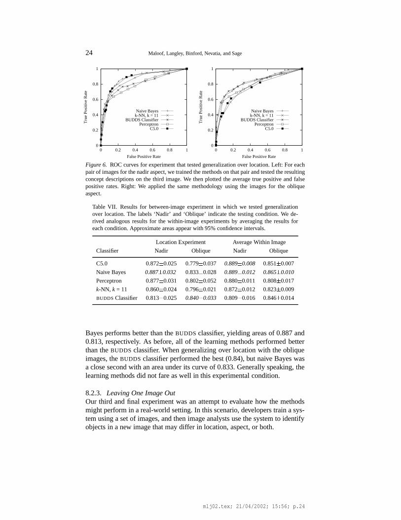
8.2.2. Generalizing over LocationA second experiment examined generalization over location. To this end, wetrained the learning methods on pairs of images from one aspect and tested onthe third image from the same aspect. As an example, for the nadir images,one of the three learning runs involved training on rooftop candidates fromImages 1 and 3, then testing on candidates from Image 5. We then ran eachof the algorithms across a range of costs, measuring the false positive andtrue positive rates. We plotted the averages of these measures across all threelearning runs for one aspect in an ROC curve, as shown in Figure 6.

In this context, we again see evidence that the oblique images presenteda more difficult recognition task than the nadir aspect, since areas for theoblique images are less than those for the nadir images. Comparing the be-havior of the various methods, Table VII shows that for the nadir aspect, naive

mlj02.tex; 21/04/2002; 15:56; p.23


0

0.2

0.4

0.6

0.8

1

0 0.2 0.4 0.6 0.8 1

Tru

e Po

sitiv

e R

ate

False Positive Rate



C5.0

0

0.2

0.4

0.6

0.8

1

0 0.2 0.4 0.6 0.8 1

Tru

e Po

sitiv

e R

ate

False Positive Rate



C5.0

Figure 6. ROC curves for experiment that tested generalization over location. Left: For eachpair of images for the nadir aspect, we trained the methods on that pair and tested the resultingconcept descriptions on the third image. We then plotted the average true positive and falsepositive rates. Right: We applied the same methodology using the images for the obliqueaspect.

Table VII. Results for between-image experiment in which we tested generalizationover location. The labels ‘Nadir’ and ‘Oblique’ indicate the testing condition. We de-rived analogous results for the within-image experiments by averaging the results foreach condition. Approximate areas appear with 95% confidence intervals.

Location Experiment Average Within Image

Classifier Nadir Oblique Nadir Oblique

C5.0 0.872 � 0.025 0.779 � 0.037 0.889 � 0.008 0.851 � 0.007

Naive Bayes 0.887 � 0.032 0.833 � 0.028 0.889 � 0.012 0.865 � 0.010

Perceptron 0.877 � 0.031 0.802 � 0.052 0.880 � 0.011 0.808 � 0.017

k-NN, k = 11 0.860 � 0.024 0.796 � 0.021 0.872 � 0.012 0.823 � 0.009


Bayes performs better than the BUDDS classifier, yielding areas of 0.887 and0.813, respectively. As before, all of the learning methods performed betterthan the BUDDS classifier. When generalizing over location with the obliqueimages, the BUDDS classifier performed the best (0.84), but naive Bayes wasa close second with an area under its curve of 0.833. Generally speaking, thelearning methods did not fare as well in this experimental condition.

8.2.3. Leaving One Image OutOur third and final experiment was an attempt to evaluate how the methodsmight perform in a real-world setting. In this scenario, developers train a sys-tem using a set of images, and then image analysts use the system to identifyobjects in a new image that may differ in location, aspect, or both.

mlj02.tex; 21/04/2002; 15:56; p.24


0

0.2

0.4

0.6

0.8

1

0 0.2 0.4 0.6 0.8 1

Tru

e Po

sitiv

e R

ate

False Positive Rate



C5.0

Figure 7. ROC curve for the experiment in which we left each image out as a test imageand trained using the remaining five images. Naive Bayes produced the curve with the largestarea, but all of the other learning methods yielded curves larger in area than that of the BUDDS

classifier.

Table VIII. Results for the experiment in which we left images out fortesting and trained using the remaining five images. We held out eachimage, each nadir image, and each oblique image. Average areas underthe ROC curve appear with 95% confidence intervals.

Area under ROC Curve

Classifier Each Nadir Oblique

Naive Bayes 0.887 � 0.040 0.911 � 0.065 0.863 � 0.051

Perceptron 0.874 � 0.044 0.909 � 0.071 0.855 � 0.082

C5.0 0.854 � 0.042 0.880 � 0.062 0.828 � 0.059

k-NN (k � 11) 0.845 � 0.043 0.872 � 0.075 0.819 � 0.042

BUDDS Classifier 0.828 � 0.039 0.829 � 0.068 0.828 � 0.069

For this experiment, we evaluated the learning methods under three exper-imental conditions. In the first, we selected each of the images for testingand used the remaining images for training. In the second, we proceededsimilarly, but left out each of the nadir images. In the third, we left out eachof the oblique images. For each data set in each condition, we applied eachlearning method, testing the resulting classifiers over a range of error costson rooftop candidates from the test image, with each method producing anROC curve. We repeated this procedure for each image remaining in the setand averaged over the runs. Plots of the ROC curves for the first conditionappear in Figure 7. We also approximated the area under the curves for allthree conditions and computed 95% confidence intervals, and these measuresappear in Table VIII.

mlj02.tex; 21/04/2002; 15:56; p.25


As in the previous experiments, the learning methods generally outper-formed the handcrafted BUDDS classifier, which produced a curve with anarea of roughly 0.828 for each of the three experimental conditions. NaiveBayes, as in the previous settings, performed the best with an area under theROC curve of 0.887 for the first condition, 0.911 for the condition in whichwe held our nadir images, and 0.863 for the condition in which we held outoblique images. In this experiment, we again see evidence that the obliqueimages posed a more difficult learning problem than the nadir images. Finally,for the condition in which we left out each of the oblique images, naive Bayesand the perceptron outperformed the BUDDS classifiers, but this was not trueof C5.0 and k-NN, for k � 11.

8.2.4. SummaryIn experiments testing performance on unseen images, the results of the naiveBayesian classifier support our main hypothesis. In most experimental condi-tions, this method fared better than the BUDDS linear classifier. On the otherhand, we were disappointed that the learning methods performed worse thanthe BUDDS classifier in the hardest experimental condition: generalizing tonew locations with an oblique viewpoint, which went against our originalexpectations.

Recall that we also anticipated that generalizing across images wouldgive lower accuracies than generalizing within images. To test this hypoth-esis, we must compare the results from these experiments with those fromthe within-image experiments. Simple calculation shows that for the within-image condition, naive Bayes produced an average ROC area of 0.889 forthe nadir images and 0.865 for the oblique images. Similarly, C5.0 aver-aged 0.889 for the nadir images and 0.851 for the oblique images. Most ofthese average areas, which appear in the two rightmost columns of Tables VIand VII, are larger than the analogous areas that resulted when these methodsgeneralized across location and aspect. One exception is that naive Bayes,C5.0, and the perceptron performed almost as well when generalizing overlocation for the nadir image (see Table VII), but the results generally supportour prediction.

Finally, in perhaps the most realistic experimental condition in which wetrained methods on a collection of images and tested on new images, thelearning methods, especially naive Bayes, performed quite well. Althoughthis outcome supports our hypothesis that learning methods can outperformhandcrafted heuristics, it highlights the need for incorporating learning mech-anisms into systems for image analysis.

mlj02.tex; 21/04/2002; 15:56; p.26


0

0.2

0.4

0.6

0.8

1

0 0.2 0.4 0.6 0.8 1

Tru

e Po

sitiv

e R

ate

False Positive Rate



C5.0

Figure 8. Results from Experiment I plotted in an ROC graph.

9. Discussion of the Experimental Results

In the first experiment, we evaluated the four learning methods traditionally,without taking into account the cost of errors and using accuracy as our mea-sure of performance. Based on these results, there was no clear choice forthe best performing classifier. C5.0 did achieve the highest overall predictiveaccuracy, but naive Bayes, while doing poorly overall, performed the best onthe most important class, the rooftops. Nevertheless, naive Bayes’ true posi-tive rate was not significantly better than the handcrafted BUDDS classifier’s,the method we were attempting to improve upon.

If we plot the true positive and false positive rates from the first experimentin an ROC graph, as shown in Figure 8, we gain additional insights into therelative performances of the methods. We see that each of the points lie onsome unknown ROC curve and that the first experiment charted little of theROC space.

In the second experiment, because of an improved evaluation method-ology that involved cost-sensitive learning algorithms, ROC analysis, and asingle measure of performance—area under the ROC curve—we had a muchbetter understanding of how each method performed. Although we may havebeen able to conclude based on the results of the first experiment that C5.0was the best method for detecting rooftops, the results from the second ex-periment more clearly demonstrated this fact, and we were able to draw thisconclusion with greater certainty.

Comparing the performances of naive Bayes in the first and second exper-iments, we see how the ROC methodology elucidated important but hiddenaspects of performance. Based on the results from the first experiment, weconcluded that the performance of naive Bayes was no better than that ofthe BUDDS classifier. Yet, the results from the second experiment revealeda very different picture and showed that over a range of costs and in an

mlj02.tex; 21/04/2002; 15:56; p.27


important region of the ROC space (i.e, where the true positive rate is greaterthan 0.6 and the false positive rate is less than 0.4), naive Bayes significantlyoutperformed the BUDDS classifier.

As we discussed previously, the skewed distribution of the data set con-siderably affected the performance of the perceptron, which simply learnedto predict the negative class, but did not affect as greatly the performanceof naive Bayes, which found a more acceptable trade-off between the falsepositive and true positive rates. We speculate that each learning method op-erates under the influence of an inherent but unknown set of cost parametersassociated with its inductive bias. These differences may have caused naiveBayes to be less effected than the perceptron by the skewed distribution ofthe data set and may partially account for the differences in performance ofthe methods in Experiment I.

Although the perceptron did quite poorly in the first experiment, the resultsfrom the second experiment showed ultimately that its ROC curve did indeeddominate that of the BUDDS classifier. Therefore, a problem with using accu-racy as the sole measure of performance is that under certain conditions, wemay conclude that a given method is superior to other methods, when in fact,the ROC curves for the same methods, for the same task, reveal completelydifferent phenomena.

From the within-learning experiments, in which we trained and tested thelearning methods using data derived from the same image, it was apparentthat at least one machine learning method, naive Bayes, showed promise ofimproving the detection of rooftops over the handcrafted linear classifier. Theresults from this experiment also established baseline performance conditionsfor the methods because they controlled for differences in aspect and location.

In an effort to test the learning methods for their ability to generalize to un-seen images, we found that rooftop detection for oblique images posed a moredifficult problem than for nadir images. This could be because BUDDS wasinitially developed using nadir images and then extended to handle obliqueimages. Thus, the features may be biased toward nadir-view rooftops. A morelikely explanation is that oblique images are simply harder than nadir images.As we indicated previously, oblique images yield more negative examples,and we believe these additional negative examples pose a more difficult learn-ing problem. Nevertheless, under all but one circumstance, the performanceof naive Bayes was better than that of the handcrafted linear classifier.

10. Related Work

Research on learning in computer vision has become increasingly commonin recent years. Some work in visual learning takes an image-based approach(e.g., Beymer & Poggio, 1996), in which the images themselves, usually nor-

mlj02.tex; 21/04/2002; 15:56; p.28


malized or transformed in some way, are used as input to a learning process,which is responsible for forming the intermediate representations necessaryto transform the pixels into a decision or classification. Researchers haveused this approach extensively for face and gesture recognition (e.g., Chan,Nasrabadi, & Mirelli, 1996; Gutta, Huang, Imam, & Weschler, 1996; Osuna,Freund, & Girosi, 1997; Segen, 1994), although it has seen other applicationsas well (e.g., Nayar & Poggio, 1996; Pomerleau, 1996; Viola, 1993).

A slightly different approach relies on handcrafted vision routines to ex-tract relevant image features, based on intensity or shape properties, thenrecognizes objects using learned classifiers that take these features as in-puts. For example, Shepherd (1983) used decision-tree induction to constructclassifiers for chocolate shapes in an industrial vision application. Cromwelland Kak (1991) took a similar approach to recognizing electrical compo-nents, such as transistors, resistors, and capacitors. Maloof and Michalski(1997) examined various methods of learning shape characteristics for detect-ing blasting caps in X-ray images, whereas additional work (Maloof, Duric,Michalski, & Rosenfeld, 1996) discussed learning in a multi-step vision sys-tem for the same detection problem.

Researchers have also investigated structural approaches, which we di-vide into two categories: model-based and hierarchical. The former approachrelies on features computed from images, but combines elementary visualconstructs extracted from images to form higher-level constructs, which thesystem compares to a database of object models. Connell and Brady (1987)incorporated learning into a model-based vision system. Using the vision taskof classifying airplanes from aerial views, their method converts objects intosemantic networks, which serve as training examples for a learning processthat produces generalized object descriptions. However, the authors do notappear to have tested experimentally their algorithm’s ability to classify ob-jects in new images. Binford, Levitt, and colleagues, in a series of papers,examined Bayesian methods for inference in a model-based system usinggeneralized cylinders as the primitive (Binford, Levitt, & Mann, 1987; Levitt,Agosta, & Binford, 1989).

Hierarchical vision systems work similarly to model-based systems buteliminate the requirement of a model-base and model matching by usingperceptual grouping operations to combine visual constructs and by usingheuristics to select the most promising constructs for further processing (Mo-han & Nevatia, 1989). Grouping and selection continues until the systemforms a view-dependent representation of the object detected in the image.Researchers have successfully applied this approach to building detection insingle images (Lin & Nevatia, 1998) and in multiple images (Noronha &Nevatia, 1997). Recent work on learning within this framework has concen-trated on single levels of the hierarchy (Maloof, Langley, Binford, & Nevatia,1998; Maloof et al., 1997; Kim & Nevatia, 1999, 2000), with two exceptions

mlj02.tex; 21/04/2002; 15:56; p.29


being that of Maloof (2000) and of Pope and Lowe (2000). Finally, Sarkarand Soundararajan (2000) used learning automata to acquire the knowledgenecessary for perceptual grouping.

Several researchers have also investigated learning for three-dimensionalvision systems. Papers by Conklin (1993), Cook, Hall, Stark, and Bowyer(1993), Woods, Cook, Hall, Bowyer, and Stark (1995), Provan, Langley, andBinford (1996), and Sengupta and Boyer (1993) all describe inductive ap-proaches aimed at improving object recognition. The objective of this ap-proach is to learn the three-dimensional structure that characterizes an objector object class, rather than its appearance. Another line of research, whichfalls midway between this approach and image-based schemes, instead at-tempts to learn a small set of characteristic views, each of which can be usedto recognize an object from a different perspective (e.g., Gros, 1993; Pope &Lowe, 1996).

Much of the research on visual learning uses images of scenes or objectsviewed at eye level (e.g., Draper, 1997; Sarkar & Soundararajan, 2000; Teller& Veloso, 1997). One exception is the SKICAT system (Fayyad, Smyth,Burl, & Perona, 1996), which catalogs celestial objects, such as galaxiesand stars, using images from the Second Palomar Observatory Sky Survey.A related system, JARTool (Fayyad et al., 1996), also analyzes aerial images,in this case to detect Venusian volcanos, using synthetic aperture radar on theMagellan spacecraft.

Burl and his colleagues extended JARTool by using an ensemble of 48neural networks to improve performance (Burl et al., 1998). Using ROCcurves, they demonstrated that the ensemble achieved better performancethan either the individually learned classifiers or the one used originally inJARTool. They also documented some of the difficulties associated with ap-plying machine learning techniques to real-world problems, such as featureselection and instance labeling, which were similar to those we encountered.

Kubat, Holte, and Matwin (1998) used the SHRINK system (Kubat, Holte,& Matwin, 1996) to detect oil spills in overhead images. They too dealt withimbalanced data sets, but also coped with a scarcity of data that was notpresent in our domain. Luckily, we were able to select images that containedsufficient concentrations of buildings, but oil spills, especially those capturedin satellite images, proved to be a rarity. Their images from a synthetic aper-ture radar covered 3500 square kilometers and contained as few as two oilspills. Although they had more images than we—nine versus our six—oursystem extracted many more objects: 17,829 positive and negative examplesof rooftops as compared to 937 positive and negative examples of oil spills.Interestingly, the relative proportion of positive examples in these data setswas identical: approximately 4.38%.

Finally, Draper (1996) conducted a careful study of learning in the contextof analyzing aerial images. His approach adapted methods for reinforcement

mlj02.tex; 21/04/2002; 15:56; p.30


learning to assign credit in multi-stage recognition procedure (for softwaresimilar to BUDDS), then used an induction method (back-propagation in neu-ral networks) to learn conditions on operator selection. He presented initialresults for detecting rooftops as part of the RADIUS project (Firschein &Strat, 1997), which we discussed previously in Section 2. Our frameworkshares some features with Draper’s approach, but assumes that learning isdirected by feedback from a human expert. We predict that our supervisedmethod will be more computationally tractable than his use of reinforcementlearning, which is well known for its high complexity. Our approach doesrequire more interaction with users, but we believe this interaction will beunobtrusive if cast within the context of an advisory system for image analy-sis. Indeed, we have recently formulated a design for incorporating machinelearning algorithms into hierarchical vision systems, and preliminary resultsfor simple, compositional objects are encouraging (Maloof, 2000).

Interest in cost-sensitive learning and in ROC analysis has become in-creasingly common in recent years, and our work along these lines has someprecedents. We have already mentioned the work of Pazzani and his col-leagues (Pazzani et al., 1994), who used a hypothetical cost analysis andconstructed minimal-cost classifiers. Similarly, Draper, Brodley, and Utgoff(1994) incorporated the cost of errors into their algorithm for constructing andpruning multivariate decision trees. They tested this approach on the task oflabeling pixels from outdoor images for use by a road-following vehicle. Theydetermined that in this context, labeling a road pixel as non-road was morecostly than the reverse, and showed experimentally that their method couldreduce such errors on novel test pixels. Woods, Kegelmeyer, and Bowyer(1997), as well as Rowley, Baluja, and Kanade (1996), reported similar worktaking into account the cost of errors.

Researchers have begun using ROC analysis to measure performance ofclassifiers when costs are unknown or when data sets are skewed. Bradley(1997) incorporated mechanisms to adjust the decision threshold of severallearning algorithms and used ROC analysis to measure performance on sev-eral UCI data sets (Blake & Merz, 1998). Provost et al. (1998) conducted asimilar study but emphasized the problems with using accuracy as a measureof performance. We have used ROC analysis to measure the ability of variousclassifiers to generalize on a rooftop detection task when unseen images var-ied in aspect and in location (Maloof et al., 1998). As mentioned previously,we have also conducted a comparative study that examined the errors expertsmade when labeling training data using our visual interface and the effect ofsuch errors on learning (Ali et al., 1998).

In terms of the statistical analysis of ROC curves, Bradley (1997) usedANOVA and Duncan’s test to analyze the means and subgroups of means,respectively, of classifier performance, as measured by area under the curve.However, this analysis treats a classifier’s performance on an individual case

mlj02.tex; 21/04/2002; 15:56; p.31


in the testing set as a fixed effect, and as a result, we cannot generalize theseresults to the population from which the test cases were drawn (Metz, 1989).We can generalize them only to the population of test sets. Furthermore,empirical results from a Monte Carlo simulation suggest that, since ANOVAdoes not adequately account for case-sample variance, especially when sam-ple sizes are small, it fails to reject the null hypothesis more frequently thanmethods designed to account for this variance. Therefore, ANOVA may beoverly optimistic for machine-learning experiments using area under the ROCcurve as the performance metric (Maloof, 2002).

Estimating or accounting for case-sample variance can be difficult, but aswe have described, Dorfman et al. (1992) detailed a methodology in whichone uses the Jackknife method (Hinkley, 1983) to account for case-samplevariance and then applies traditional ANOVA to test significance. Recently,Beiden, Wagner, and Campbell (2000) proposed a nonparametric methodfor comparing means of areas that involves conducting a series of bootstrapexperiments to estimate components of variance, like the case-sample vari-ance. Although developed for human-reader experiments in medical imaging,researchers have begun to apply this method to the analysis of learning al-gorithms (Beiden, Maloof, & Wagner, 2002; Maloof, Beiden, & Wagner,2002). There has also been work on the analysis of portions of ROC curves(Thompson & Zucchini, 1986; Woods et al., 1997) and in situations in whichno single ROC curve dominates in all parts of the ROC space (e.g., Provost &Fawcett, 1997). Researchers have also proposed extensions to ROC analysisfor the case of multiple decision categories (Hand & Till, 2001; Mossman,1999; Swets & Pickett, 1982).

11. Concluding Remarks

Although this study has provided some insight into the role of cost-sensitivealgorithms and ROC analysis in systems for image understanding, much stillremains to be done. For example, we may want to consider other measures ofperformance that take into account the presence of multiple valid candidatesfor a given rooftop. Classifying one of these candidates correctly is sufficientfor the purpose of image analysis.

As we mentioned earlier, in order to automate the collection of trainingdata for learning, we also hope to integrate learning routines into BUDDS. Thissystem was not designed initially to be interactive, but we intend to modifyit so that the image analyst can accept or reject recommendations made bythe image understanding system, generating training data in the process. Atintervals the system would invoke its learning algorithms, producing revisedknowledge that would alter the system’s behavior in the future and, hopefully,

mlj02.tex; 21/04/2002; 15:56; p.32


reduce the user’s need to make corrections. The interactive labeling systemdescribed in Section 5 could serve as an initial model for this interface.

Although the rooftop selection stage was a natural place to start in ap-plying our methods, we intend to work at both earlier and later levels of thebuilding detection process. The goal here is not only to increase classificationaccuracy, which could be handled entirely by candidate selection, but alsoto reduce the complexity of processing by removing poor candidates beforethey are aggregated into larger structures. With this aim in mind, we plan toextend our work to all levels of the image understanding process. We mustaddress a number of issues before we can make progress on these otherstages. One involves identifying the cost of different errors at each level,and taking this into account in our modified induction algorithms. Anotherconcerns whether we should use the same induction algorithm at each levelor use different methods at each stage. We could also use multiple methodsat each level and apply ensemble methods, such as stacking (Wolpert, 1992)or bagging (Breiman, 1996), to produce a single decision and to take intoaccount contextual cues, such as aspect.

In conclusion, our studies suggest that machine learning has an importantrole to play in improving the accuracy and the robustness of image analysissystems. We need to extend learning to additional levels of the image under-standing process, and before we can build a system that truly aids the humanimage analyst, we must further develop unobtrusive ways to collect trainingdata to support learning. Nevertheless, as more and more vision systems relyon learning and adaptive mechanisms, it will become increasingly importantto properly measure the performance of such systems.

Appendix

A. Generating ROC Curves

We are aware of three methods of generating ROC curves (Metz, 1978). First,if we modify the performance element of a learning method to produce anumeric rating for each test case—for example, with naive Bayes, we mightselect the posterior probability of the positive class—then we can use a para-metric approach by assuming a binormal distribution (i.e., observations ofeach of the two classes are normally distributed) and fitting the ROC curveof maximum likelihood (Dorfman & Alf, 1969). It is then a simple matter ofcomputing the area under this curve (Bamber, 1975; Thompson & Zucchini,1986).

Second, with such ratings, we can also use a nonparametric approach inwhich we map the sorted case ratings into, say, 10–12 discrete categories(Wagner, Beiden, & Metz, 2001) and use the number of actually positive

mlj02.tex; 21/04/2002; 15:56; p.33


cases and actually negative cases of each category to calculate the true posi-tive and false positive rates of an ROC curve.

With these points, we can use the trapezoid rule to compute the approx-imate area under the curve, A, but researchers have shown this measure tobe equal to the Mann-Whitney two-sample statistic (DeLong, DeLong, &Clarke-Peterson, 1988), which is convenient for numeric case ratings. Givenm ratings of negative cases, r � , and n ratings of positive cases, r � ,

A � 1mn

m

∑i � 1

n

∑j � 1

I � r �i r �j ��where

I � r � r � � �� 1 if r � � r � ;12 if r � � r � ;0 if r � r �

For some algorithms, it is easy to modify the performance element toproduce these ratings. For this purpose, we have used for naive Bayes theposterior probability of the positive class, for k-NN, the number of majorityvotes for the positive class, and for linear and quadratic discriminants, theoutput of the discriminant function (Maloof et al., 2002).

However, when we attempted to modify C4.5 (Quinlan, 1993) in this man-ner by using as ratings the weights that the performance element computesfor test instances, the resulting ROC curves were either degenerate or not ofthe correct area (which we established through further experimentation). Itappears the problem is that C4.5, like many learning methods, partitions therepresentation space to form decision regions with instances in each regionbeing equiprobable. If the number of decision regions is few, then there willbe little information present in the case ratings for constructing the ROCcurve.

The third method of generating ROC curves, which we used in this study,involves varying some aspect of the learning method or the experiment to biasthe learner toward one class versus the other. Unfortunately, such schemestend to be specific to a learning method (cf. Domingos, 1999) and can in-crease the running time, but include varying the prior probabilities of eachclass, the error cost of each class, the decision threshold, and the class distri-bution of examples in the training set.

In this study, we chose to introduce a mechanism into the performanceelement that adjusts the decision threshold. Once we have modified the al-gorithm in this fashion, then it should be a simple matter to select variousthresholds, to evaluate the examples in the test set at each, and to produce aset of true positive and false positive rates that form an ROC curve. Unfor-tunately, many things conspire to make selecting a set of decision thresholdsdifficult, such as the distribution of the training examples and the inductive

mlj02.tex; 21/04/2002; 15:56; p.34


bias of the learner. For instance, it can be difficult to predict which thresholdwill produce a given point on an ROC curve. A set of parameters for varyingthe decision threshold for one algorithm will not necessarily produce the sameROC curve for another algorithm. Finally, for a given algorithm and set ofdecision thresholds, different splits of the data set will yield different ROCcurves. This was especially true when we trained on nadir images and testedon oblique images.

Reluctantly, we concluded that setting these thresholds by trial and errorfor each algorithm would be necessary. We split all of the available data intosingle training (60%) and testing (40%) sets, and applied each learning algo-rithm. For each method, we began with the decision threshold implying thatmistakes on the positive class were maximally expensive, which producedthe point � 0 0 � on the ROC graph. We repeatedly added new cost parametersthat increasingly favored the positive class until the performance elementswept out a curve that was well-shaped with points distributed evenly alongits length.

This third method of generating ROC curves can be disadvantageous foralgorithms with a costly performance element, such as k-NN. We must cyclethrough the training examples, finding the k closest neighbors, for each costparameter. For our data set, this was expensive. Other methods performedquickly. For instance, the perceptron computes a simple weighted sum, andevaluating this sum for each example and over the cost parameters requiredlittle time. Nevertheless, we contend that the nonparametric method of pro-ducing ROC curves is more efficient and more principled, but as we havedescribed, it may not work well for all learning methods without significantmodification.

Acknowledgements

The authors thank Wayne Iba for assistance with naive Bayes, Dan Shapirofor discussions about decision theory, Yan Bulgak for proofreading a draft ofthe paper, Ross Quinlan for describing the cost-sensitive mechanisms in C5.0,and Andres Huertas and Andy Lin for advice and assistance in obtaining theimages and data used for experimentation. Robert Wagner provided valuablecomments regarding ROC analysis, and Sergey Beiden conducted the anal-ysis of the learning algorithms using LabMRMC. We are grateful to DougFisher and the anonymous reviewers, who provided constructive and collegialadvice that notably improved an earlier version of the manuscript. We thankthe Department of Computer Science at Georgetown University for their sup-port of this work. This research was conducted at the Institute for the Study ofLearning and Expertise and in the Computational Learning Laboratory, Cen-ter for the Study of Language and Information, at Stanford University. The

mlj02.tex; 21/04/2002; 15:56; p.35


work was supported by the Defense Advanced Research Projects Agency, un-der grant N00014-94-1-0746, administered by the Office of Naval Research,and by Sun Microsystems through a generous equipment grant.

References

Aha, D., Kibler, D., & Albert, M. (1991). Instance-based learning algorithms.Machine Learning, 6, 37–66.

Ali, K., Langley, P., Maloof, M., Sage, S., & Binford, T. (1998). Improvingrooftop detection with interactive visual learning. In Proceedings ofthe Image Understanding Workshop (pp. 479–492). San Francisco,CA: Morgan Kaufmann.

Bamber, D. (1975). The area above the ordinal dominance graph and thearea below the receiver operating characteristic graph. Journal ofMathematical Psychology, 12, 387–415.

Beiden, S., Maloof, M., & Wagner, R. (2002). Analysis of competing clas-sifiers in terms of components of variance of ROC summary accuracymeasures: Generalization to a population of trainers and a populationof testers. In Proceedings of the SPIE International Symposium onMedical Imaging: Image Processing (Vol. 4684).

Beiden, S., Wagner, R., & Campbell, G. (2000). Components-of-variancemodels and multiple-bootstrap experiments: An alternative method forrandom-effects Receiver Operating Characteristic analysis. AcademicRadiology, 7, 341–349.

Beymer, D., & Poggio, T. (1996). Image representations for visual learning.Science, 272, 1905–1909.

Binford, T., Levitt, T., & Mann, W. (1987). Bayesian inference in model-based machine vision. In Proceedings of the Third Annual Conferenceon Uncertainty in Artificial Intelligence (UAI-87) (pp. 73–97). NewYork, NY: Elsevier Science.

Blake, C., & Merz, C. (1998). UCI Repository of machine learning databases([http://www.ics.uci.edu/ mlearn/MLRepository.html]). Departmentof Information and Computer Sciences, University of California,Irvine.

Bradley, A. (1997). The use of the area under the ROC curve in the eval-uation of machine learning algorithms. Pattern Recognition, 30(7),1145–1159.

mlj02.tex; 21/04/2002; 15:56; p.36


Breiman, L. (1996). Bagging predictors. Machine Learning, 24, 123–140.

Breiman, L., Friedman, J., Olshen, R., & Stone, C. (1984). Classification andregression trees. Boca Raton, FL: Chapman & Hall/CRC Press.

Burl, M., Asker, L., Smyth, P., Fayyad, U., Perona, P., Crumpler, L., &Aubele, J. (1998). Learning to recognize volcanoes on Venus. MachineLearning, 30, 165–194.

Cardie, C., & Howe, N. (1997). Improving minority class prediction usingcase-specific feature weights. In Proceedings of the Fourteenth Inter-national Conference on Machine Learning (pp. 57–65). San Francisco,CA: Morgan Kaufmann.

Chan, L., Nasrabadi, N., & Mirelli, V. (1996). Multi-stage target recogni-tion using modular vector quantizers and multilayer perceptrons. InProceedings of the IEEE Conference on Computer Vision and PatternRecognition (CVPR ’96) (pp. 114–119). Los Alamitos, CA: IEEEPress.

Clark, P., & Niblett, T. (1989). The CN2 induction algorithm. MachineLearning, 3, 261–284.

Conklin, D. (1993). Transformation-invariant indexing and machine discov-ery for computer vision. In Papers from the the AAAI Fall Symposiumon Machine Learning in Computer Vision: What, Why, and How?Technical Report No. FS-93-04 (pp. 10–14). Menlo Park, CA: AAAIPress.

Connell, J., & Brady, M. (1987). Generating and generalizing models ofvisual objects. Artificial Intelligence, 31, 159–183.

Cook, D., Hall, L., Stark, L., & Bowyer, K. (1993). Learning combination ofevidence functions in object recognition. In Papers from the the AAAIFall Symposium on Machine Learning in Computer Vision: What, Why,and How? Technical Report No. FS-93-04 (pp. 139–143). Menlo Park,CA: AAAI Press.

Cromwell, R., & Kak, A. (1991). Automatic generation of object classdescriptions using symbolic learning techniques. In Proceedings ofthe Ninth National Conference on Artificial Intelligence (pp. 710–717).Menlo Park, CA: AAAI Press.

DeLong, E., DeLong, D., & Clarke-Peterson, D. (1988). Comparing the areasunder two or more correlated receiver operating characteristic curves:A nonparametric approach. Biometrics, 44, 837–845.

mlj02.tex; 21/04/2002; 15:56; p.37


Domingos, P. (1999). MetaCost: A general method for making classifierscost-sensitive. In Proceedings of the Fifth International Conference onKnowledge Discovery and Data Mining (pp. 155–164). New York, NY:ACM Press.

Dorfman, D., & Alf, E., Jr. (1969). Maximum likelihood estimation ofparameters of signal-detection theory and determination of confidenceintervals—rating method data. Journal of Mathematical Psychology,6, 487–496.

Dorfman, D., Berbaum, K., & Metz, C. (1992). Receiver Operating Char-acteristic rating analysis: Generalization to the population of readersand patients with the Jackknife method. Investigative Radiology, 27,723–731.

Draper, B. (1996). Learning grouping strategies for 2D and 3D objectrecognition. In Proceedings of the Image Understanding Workshop(pp. 1447–1454). San Francisco, CA: Morgan Kaufmann.

Draper, B. (1997). Learning control strategies for object recognition. InK. Ikeuchi & M. Veloso (Eds.), Symbolic visual learning (pp. 49–76).New York, NY: Oxford University Press.

Draper, B., Brodley, C., & Utgoff, P. (1994). Goal-directed classificationusing linear machine decision trees. IEEE Transactions on PatternAnalysis and Machine Intelligence, 16(9), 888–893.

Duda, R., & Hart, P. (1973). Pattern classification and scene analysis. NewYork, NY: John Wiley & Sons.

Egan, J. (1975). Signal detection theory and ROC analysis. New York, NY:Academic Press.

Ezawa, K., Singh, M., & Norton, S. (1996). Learning goal-oriented Bayesiannetworks for telecommunications risk management. In Proceedingsof the Thirteenth International Conference on Machine Learning (pp.139–147). San Francisco, CA: Morgan Kaufmann.

Fawcett, T., & Provost, F. (1997). Adaptive fraud detection. Data Miningand Knowledge Discovery, 1, 291–316.

Fayyad, U., Smyth, P., Burl, M., & Perona, P. (1996). Learning to catalogscience images. In S. Nayar & T. Poggio (Eds.), Early visual learning(pp. 237–268). New York, NY: Oxford University Press.

Firschein, O., & Strat, T. (Eds.). (1997). RADIUS: Image understanding forimagery intelligence. San Francisco, CA: Morgan Kaufmann.

mlj02.tex; 21/04/2002; 15:56; p.38


Freund, Y., & Schapire, R. (1996). Experiments with a new boosting al-gorithm. In Proceedings of the Thirteenth International Conferenceon Machine Learning (pp. 148–156). San Francisco, CA: MorganKaufmann.

Freund, Y., Seung, H., Shamir, E., & Tishby, N. (1997). Selective samplingusing the Query by Committee algorithm. Machine Learning, 28, 133–168.

Green, D., & Swets, J. (1974). Signal detection theory and psychophysics.New York, NY: Robert E. Krieger Publishing.

Gros, P. (1993). Matching and clustering: Two steps towards automatic objectmodel generation in computer vision. In Papers from the the AAAI FallSymposium on Machine Learning in Computer Vision: What, Why, andHow? Technical Report No. FS-93-04 (pp. 40–44). Menlo Park, CA:AAAI Press.

Gutta, S., Huang, J., Imam, I., & Weschler, H. (1996). Face and hand ges-ture recognition using hybrid classifiers. In Proceedings of the SecondInternational Conference on Automatic Face and Gesture Recognition(pp. 164–169). Los Alamitos, CA: IEEE Press.

Hand, D., & Till, R. (2001). A simple generalisation of the area underthe ROC curve for multiple class classification problems. MachineLearning, 45, 171–186.

Hanley, J., & McNeil, B. (1982). The meaning and use of the area under aReceiver Operating Characteristic (ROC) curve. Radiology, 143, 29–36.

Hinkley, D. (1983). Jackknife methods. In S. Kotz, N. Johnson, & C. Read(Eds.), Encyclopedia of statistical sciences (Vol. 4, pp. 280–287). NewYork, NY: John Wiley & Sons.

John, G., & Langley, P. (1995). Estimating continuous distributions inBayesian classifiers. In Proceedings of the Eleventh Conference onUncertainty in Artificial Intelligence (pp. 338–345). San Francisco,CA: Morgan Kaufmann.

Keppel, G., Saufley, W., & Tokunaga, H. (1992). Introduction to design andanalysis (2nd ed.). New York, NY: W.H. Freeman.

Kim, Z., & Nevatia, R. (1999). Uncertain reasoning and learning for featuregrouping. Computer Vision and Image Understanding, 76(3), 278–288.

mlj02.tex; 21/04/2002; 15:56; p.39


Kim, Z., & Nevatia, R. (2000). Learning Bayesian networks for diverse andvarying numbers of evidence sets. In Proceedings of the SeventeenthInternational Conference on Machine Learning (pp. 479–486). SanFrancisco, CA: Morgan Kaufmann.

Kubat, M., Holte, R., & Matwin, S. (1996). Learning when negative examplesabound. In Proceedings of the 1997 European Conference on MachineLearning.

Kubat, M., Holte, R., & Matwin, S. (1998). Machine learning for thedetection of oil spills in satellite images. Machine Learning, 30,195–215.

Kubat, M., & Matwin, S. (1997). Addressing the curse of imbalancedtraining sets: One-sided selection. In Proceedings of the FourteenthInternational Conference on Machine Learning (pp. 179–186). SanFrancisco, CA: Morgan Kaufmann.

Langley, P., Iba, W., & Thompson, K. (1992). An analysis of Bayesian clas-sifiers. In Proceedings of the Tenth National Conference on ArtificialIntelligence (pp. 223–228). Menlo Park, CA: AAAI Press.

Langley, P., & Simon, H. (1995). Applications of machine learning and ruleinduction. Communications of the ACM, 38(11), 54–64.

Levitt, T., Agosta, J., & Binford, T. (1989). Model-based influence diagramsfor machine vision. In Proceedings of the Fifth Annual Conferenceon Uncertainty in Artificial Intelligence (UAI-89) (pp. 371–388). NewYork, N.Y.: Elsevier Science.

Lewis, D., & Catlett, J. (1994). Heterogeneous uncertainty sampling forsupervised learning. In Proceedings of the Eleventh InternationalConference on Machine Learning (pp. 148–156). San Francisco, CA:Morgan Kaufmann.

Lin, C., & Nevatia, R. (1998). Building detection and description from asingle intensity image. Computer Vision and Image Understanding,72(2), 101–121.

Maloof, M. (2000). An initial study of an adaptive hierarchical visionsystem. In Proceedings of the Seventeenth International Conferenceon Machine Learning (pp. 567–573). San Francisco, CA: MorganKaufmann.

Maloof, M. (2002). On machine learning, ROC analysis, and statisticaltests of significance. In Proceedings of the Sixteenth InternationalConference on Pattern Recognition. Los Alamitos, CA: IEEE Press.

mlj02.tex; 21/04/2002; 15:56; p.40


Maloof, M., Beiden, S., & Wagner, R. (2002). Analysis of com-peting classifiers in terms of components of variance of ROCaccuracy measures (Technical Report No. CS-02-01). Washing-ton, DC: Department of Computer Science, Georgetown University.(http://www.cs.georgetown.edu/ maloof/pubs/cstr-02-01.html)

Maloof, M., Duric, Z., Michalski, R., & Rosenfeld, A. (1996). Recognizingblasting caps in X-ray images. In Proceedings of the Image Under-standing Workshop (pp. 1257–1261). San Francisco, CA: MorganKaufmann.

Maloof, M., Langley, P., Binford, T., & Nevatia, R. (1998). Generalizing overaspect and location for rooftop detection. In Proceedings of the FourthIEEE Workshop on Applications of Computer Vision (WACV ’98) (pp.194–199). Los Alamitos, CA: IEEE Press.

Maloof, M., Langley, P., Binford, T., & Sage, S. (1998). Learning to detectrooftops in overhead imagery (Technical Report No. 98-1). Palo Alto,CA: Institute for the Study of Learning and Expertise.

Maloof, M., Langley, P., Sage, S., & Binford, T. (1997). Learning to detectrooftops in aerial images. In Proceedings of the Image UnderstandingWorkshop (pp. 835–845). San Francisco, CA: Morgan Kaufmann.

Maloof, M., & Michalski, R. (1997). Learning symbolic descriptions ofshape for object recognition in X-ray images. Expert Systems withApplications, 12(1), 11–20.

Metz, C. (1978). Basic principles of ROC analysis. Seminars in NuclearMedicine, VIII(4), 283–298.

Metz, C. (1989). Some practical issues of experimental design and dataanalysis in radiological ROC studies. Investigative Radiology, 24, 234–245.

Michalski, R., Mozetic, I., Hong, J., & Lavrac, H. (1986). The multi-purposeincremental learning system AQ15 and its testing application to threemedical domains. In Proceedings of the Fifth National Conference onArtificial Intelligence (pp. 1041–1045). Menlo Park, CA: AAAI Press.

Miller, D., & Uyar, H. (1997). A mixture of experts classifier with learningbased on both labeled and unlabeled data. In M. Mozer, M. Jordan, &T. Petsche (Eds.), Advances in neural information processing systems(Vol. 9). Cambridge, MA: MIT Press.

mlj02.tex; 21/04/2002; 15:56; p.41


Mohan, R., & Nevatia, R. (1989). Using perceptual organization to extract3-D structures. IEEE Transactions on Pattern Analysis and MachineIntelligence, 11(11), 1121–1139.

Mossman, D. (1999). Three-way ROCs. Medical Decision Making, 19,78–89.

Nayar, S., & Poggio, T. (Eds.). (1996). Early visual learning. New York,NY: Oxford University Press.

Noronha, S., & Nevatia, R. (1997). Detection and description of buildingsfrom multiple aerial images. In Proceedings of the IEEE Conference onComputer Vision and Pattern Recognition (CVPR ’97) (pp. 588–594).Los Alamitos, CA: IEEE Press.

Osuna, E., Freund, R., & Girosi, F. (1997). Training Support Vector Ma-chines: An application to face detection. In Proceedings of the IEEEConference on Computer Vision and Pattern Recognition (CVPR ’97)(pp. 130–136). Los Alamitos, CA: IEEE Press.

Pazzani, M., Merz, C., Murphy, P., Ali, K., Hume, T., & Brunk, C. (1994).Reducing misclassification costs. In Proceedings of the Eleventh In-ternational Conference on Machine Learning (pp. 217–225). SanFrancisco, CA: Morgan Kaufmann.

Pomerleau, D. (1996). Neural network vision for robot driving. In S. Nayar& T. Poggio (Eds.), Early visual learning (pp. 161–181). New York,NY: Oxford University Press.

Pope, A., & Lowe, D. (1996). Learning probabilistic appearance modelsfor object recognition. In S. Nayar & T. Poggio (Eds.), Early visuallearning (pp. 67–97). New York, NY: Oxford University Press.

Pope, A., & Lowe, D. (2000). Probabilistic models of appearance for 3-Dobject recognition. International Journal of Computer Vision, 40(2),149–167.

Provan, G., Langley, P., & Binford, T. (1996). Probabilistic learning ofthree-dimensional object models. In Proceedings of the Image Un-derstanding Workshop (pp. 1403–1413). San Francisco, CA: MorganKaufmann.

Provost, F., & Fawcett, T. (1997). Analysis and visualization of classifierperformance: Comparison under imprecise class and cost distributions.In Proceedings of the Third International Conference on KnowledgeDiscovery and Data Mining (pp. 43–48). Menlo Park, CA: AAAIPress.

mlj02.tex; 21/04/2002; 15:56; p.42


Provost, F., Fawcett, T., & Kohavi, R. (1998). The case against accu-racy estimation for comparing induction algorithms. In Proceedingsof the Fifteenth International Conference on Machine Learning (pp.445–453). San Francisco, CA: Morgan Kaufmann.

Quinlan, J. (1993). C4.5: Programs for machine learning. San Francisco,CA: Morgan Kaufmann.

Rowley, H., Baluja, S., & Kanade, T. (1996). Neural network-based facedetection. In Proceedings of the IEEE Conference on Computer Visionand Pattern Recognition (CVPR ’96) (pp. 203–208). Los Alamitos,CA: IEEE Press.

Sarkar, S., & Soundararajan, P. (2000). Supervised learning of large percep-tual organization: Graph spectral partitioning and learning automata.IEEE Transactions on Pattern Analysis and Machine Intelligence,22(5), 504–525.

Segen, J. (1994). GEST: A learning computer vision system that recognizeshand gestures. In R. Michalski & G. Tecuci (Eds.), Machine learning:A multistrategy approach (Vol. 4, pp. 621–634). San Francisco, CA:Morgan Kaufmann.

Sengupta, K., & Boyer, K. (1993). Incremental model base updating: Learn-ing new model sites. In Papers from the the AAAI Fall Symposiumon Machine Learning in Computer Vision: What, Why, and How?Technical Report No. FS-93-04 (pp. 1–5). Menlo Park, CA: AAAIPress.

Shepherd, B. (1983). An appraisal of a decision tree approach to image clas-sification. In Proceedings of the Eighth International Joint Conferenceon Artificial Intelligence (pp. 473–475). San Francisco, CA: MorganKaufmann.

Soderland, S., & Lehnert, W. (1994). Corpus-driven knowledge acquisitionfor discourse analysis. In Proceedings of the Twelfth National Confer-ence on Artificial Intelligence (pp. 827–832). Menlo Park, CA: AAAIPress.

Swets, J. (1988). Measuring the accuracy of diagnostic systems. Science,240, 1285–1293.

Swets, J., & Pickett, R. (1982). Evaluation of diagnostic systems: Methodsfrom signal detection theory. New York, NY: Academic Press.

mlj02.tex; 21/04/2002; 15:56; p.43


Teller, A., & Veloso, M. (1997). PADO: A new learning architecture forobject recognition. In K. Ikeuchi & M. Veloso (Eds.), Symbolic visuallearning (pp. 77–112). New York, NY: Oxford University Press.

Thompson, M., & Zucchini, W. (1986). On the statistical analysis of ROCcurves. Statistics in Medicine, 18, 452–462.

Turney, P. (1995). Cost-sensitive classification: Empirical evaluation of ahybrid genetic decision tree induction algorithm. Journal of ArtificialIntelligence Research, 2, 369–409.

Viola, P. (1993). Feature-based recognition of objects. In Papers from thethe AAAI Fall Symposium on Machine Learning in Computer Vision:What, Why, and How? Technical Report No. FS-93-04 (p. 60–64).Menlo Park, CA: AAAI Press.

Wagner, R., Beiden, S., & Metz, C. (2001). Continuous versus categoricaldata for ROC analysis: Some quantitative considerations. AcademicRadiology, 8, 328–334.

Walpole, R., Myers, R., & Myers, S. (1998). Probability and statistics forengineers and scientists (6th ed.). Upper Saddle River, NJ: Prentice-Hall.

Wolpert, D. (1992). Stacked generalization. Neural Networks, 5, 241–259.

Woods, K., Cook, D., Hall, L., Bowyer, K., & Stark, L. (1995). Learningmembership functions in a function-based object recognition system.Journal of Artificial Intelligence Research, 3, 187–222.

Woods, K., Kegelmeyer, W., & Bowyer, K. (1997). Combination of mul-tiple classifiers using local accuracy estimates. IEEE Transactions onPattern Analysis and Machine Intelligence, 19(4), 405–410.

Zurada, J. (1992). Introduction to artificial neural systems. St. Paul, MN:West Publishing.

mlj02.tex; 21/04/2002; 15:56; p.44

ISLE Home Page

Documents

Transcript of ISLE Home Page