ISEN 315 Spring 2011 Dr. Gary Gaukler. Demand Uncertainty How do we come up with our random variable...
20
ISEN 315 Spring 2011 Dr. Gary Gaukler
-
Upload
hilary-peters -
Category
Documents
-
view
216 -
download
1
Transcript of ISEN 315 Spring 2011 Dr. Gary Gaukler. Demand Uncertainty How do we come up with our random variable...

ISEN 315Spring 2011
Dr. Gary Gaukler

Demand Uncertainty
How do we come up with our random variable of demand?
Recall naïve method:

Demand Uncertainty

Demand Uncertainty and Forecasting
Using the standard deviation of forecast error:

Lot Size Reorder Point Systems
Assumptions– Inventory levels are reviewed continuously (the
level of on-hand inventory is known at all times)– Demand is random but the mean and variance of
demand are constant. (stationary demand)– There is a positive leadtime, τ. This is the time that
elapses from the time an order is placed until it arrives.
– The costs are: • Set-up each time an order is placed at $K per order• Unit order cost at $c for each unit ordered• Holding at $h per unit held per unit time ( i. e., per year)• Penalty cost of $p per unit of unsatisfied demand
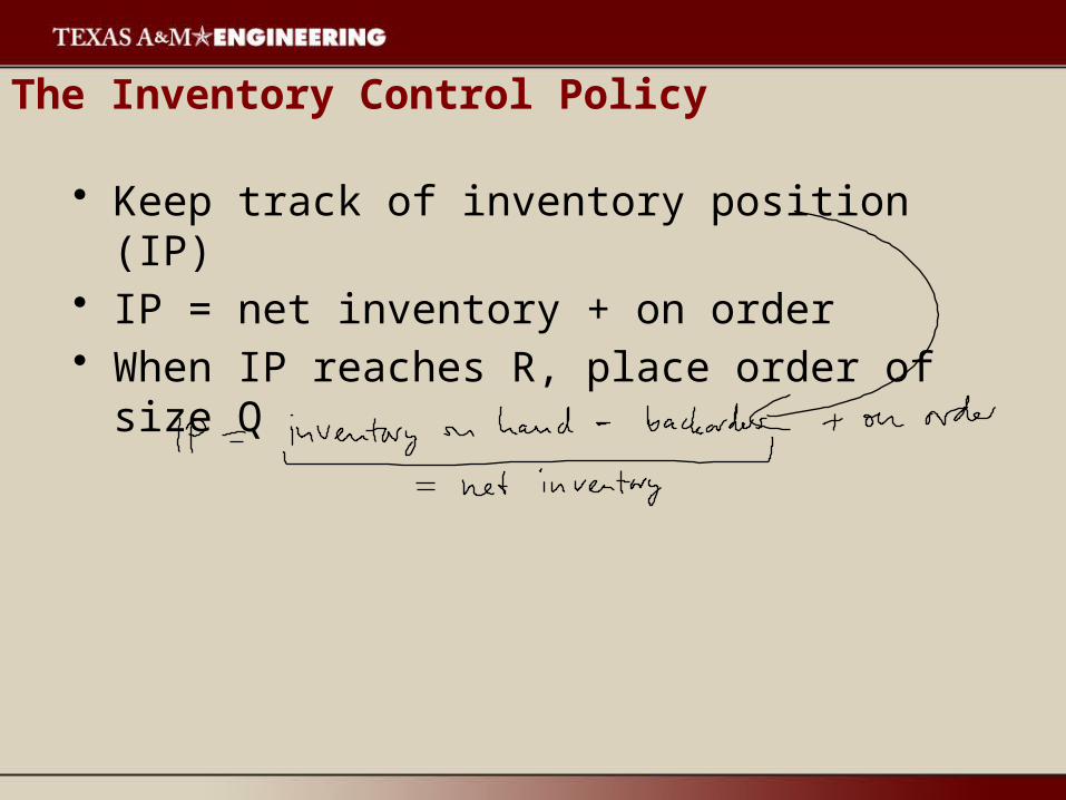
The Inventory Control Policy
• Keep track of inventory position (IP)• IP = net inventory + on order• When IP reaches R, place order of size Q

Inventory Levels

Describing Demand
• The response time of the system in this case is the time that elapses from the point an order is placed until it arrives. – The uncertainty that must be protected against is
the uncertainty of demand during the lead time. • Assume that D represents the demand during
the lead time and has probability distribution F(t).
• Although the theory applies to any form of F(t), we assume that it follows a normal distribution for calculation purposes.

Decision Variables
• Basic EOQ model:– Single decision variable Q
• Q,R model:– Q and R interdependent decision variables.
Essentially, R is chosen to protect against uncertainty of demand during the lead time, and Q is chosen to balance the holding and set-up costs

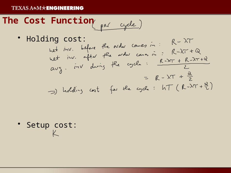
The Cost Function
Approach:• Obtain an expression of expected cost per cycle, as a
function of Q,R
• Expected annual cost =
The Cost Function
• Holding cost:
• Setup cost:

The Cost Function
• Backorder cost:
• Procurement cost:

The Cost Function
• Expected cost per cycle:
• Expected annual cost:

Derivation of Optimal Parameters

Derivation of Optimal Parameters

Review
Optimal (Q,R):

Solution Procedure
• The optimal solution procedure requires iterating between the two equations for Q and R until convergence occurs (which is generally quite fast).
• A cost effective approximation is to set Q=EOQ and find R from the second equation.
• In this class, we will use the approximation.
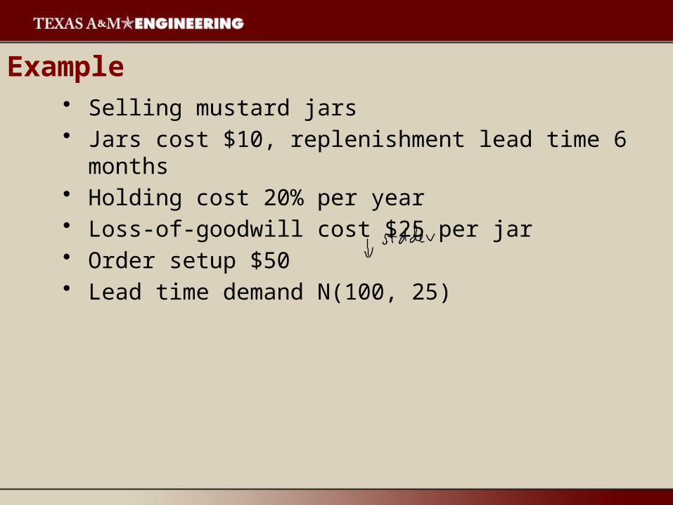
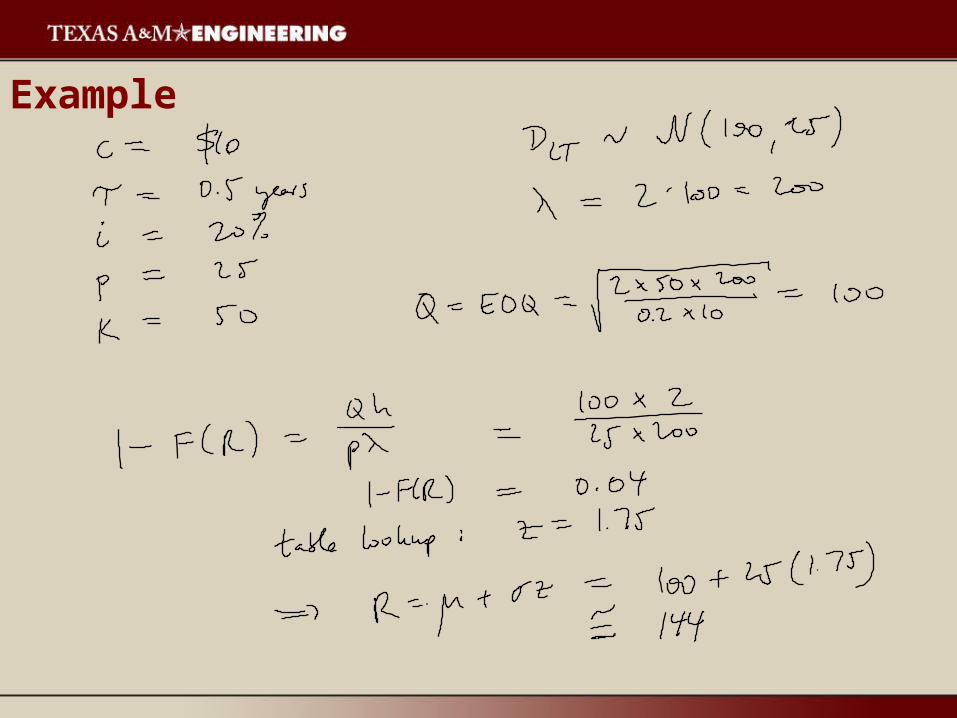
Example• Selling mustard jars• Jars cost $10, replenishment lead time 6 months• Holding cost 20% per year• Loss-of-goodwill cost $25 per jar• Order setup $50• Lead time demand N(100, 25)
Example

Example


![INTERNATIONAL ISEN SPIRITUAL EMERGENCE NETWORK · 2017. 5. 9. · ISEN SPIRITUAL EMERGENCE NETWORK . Title: SpiritualCrisisNetworkFLY-Folded [27381] Author: WensumPrint Created Date:](https://static.fdocuments.in/doc/165x107/60dc55f4ce3a8f4b09262226/international-isen-spiritual-emergence-2017-5-9-isen-spiritual-emergence-network.jpg)