A Compact Introduction to Isabelle/HOL

Tobias Nipkow

TU Munchen

– p.1

Overview

1. Introduction

2. Datatypes

3. Logic

4. Sets

– p.2

Overview of Isabelle/HOL

– p.3

System Architecture

ProofGeneral (X)Emacs based interface

Isabelle/HOL Isabelle instance for HOL

Isabelle generic theorem prover

Standard ML implementation language

– p.4

HOL

HOL = Higher-Order LogicHOL = Functional programming + Logic

HOL has• datatypes• recursive functions• logical operators (∧, −→, ∀, ∃, . . . )

HOL is a programming language!

Higher-order = functions are values, too!

– p.5

Formulae

Syntax (in decreasing priority):

form ::= (form) | term = term | ¬form

| form ∧ form | form ∨ form | form −→ form

| ∀x. form | ∃x. form

Scope of quantifiers: as far to the right as possible

Examples• ¬ A ∧ B ∨ C ≡ ((¬ A) ∧ B) ∨ C• A = B ∧ C ≡ (A = B) ∧ C• ∀ x. P x ∧ Q x ≡ ∀ x. (P x ∧ Q x)• ∀ x. ∃ y. P x y ∧ Q x ≡ ∀ x. (∃ y. (P x y ∧ Q x))

– p.6

Types and Terms

– p.7

Types

Syntax:

τ ::= (τ)

| bool | nat | . . . base types| ’a | ’b | . . . type variables| τ ⇒ τ total functions| τ × τ pairs (ascii: *)| τ list lists| . . . user-defined types

Parentheses: T1 ⇒ T2 ⇒ T3 ≡ T1 ⇒ (T2 ⇒ T3)

– p.8

Terms: Basic syntax

Syntax:

term ::= (term)

| a constant or variable (identifier)| term term function application| λx. term function “abstraction”| . . . lots of syntactic sugar

Examples: f (g x) y h (λx. f (g x))

Parantheses: f a1 a2 a3 ≡ ((f a1) a2) a3

– p.9

Terms and Types

Terms must be well-typed(the argument of every function call must be of the right type)

Notation: t :: τ means t is a well-typed term of type τ .

– p.10

Type inference

Isabelle automatically computes (“infers”) the type of eachvariable in a term.

In the presence of overloaded functions (functions withmultiple types) not always possible.

User can help with type annotations inside the term.

Example: f (x::nat)

– p.11

Currying

Thou shalt curry your functions

• Curried: f :: τ 1 ⇒ τ2 ⇒ τ

• Tupled: f’ :: τ 1 × τ2 ⇒ τ

Advantage: partial application f a1 with a1 :: τ1

– p.12

Terms: Syntactic sugar

Some predefined syntactic sugar:

• Infix: +, -, * , #, @, . . .• Mixfix: if _ then _ else _, case _ of , . . .

Prefix binds more strongly than infix:

! f x + y ≡ (f x) + y 6≡ f (x + y) !

– p.13

Base types: bool, nat, list

– p.14

Type bool

Formulae = terms of type bool

True :: boolFalse :: bool∧, ∨, . . . :: bool ⇒ bool ⇒ bool...

if-and-only-if: =

– p.15

Type nat

0 :: natSuc :: nat ⇒ nat+, *, ... :: nat ⇒ nat ⇒ nat...

! Numbers and arithmetic operations are overloaded:0,1,2,... :: ’a, + :: ’a ⇒ ’a ⇒ ’a

You need type annotations: 1 :: nat, x + (y::nat)

. . . unless the context is unambiguous: Suc z

– p.16

Type list

• [] : empty list

• x # xs: list with first element x ("head")and rest xs ("tail")

• Syntactic sugar: [x1,. . . ,xn]

Large library:hd, tl, map, size, filter, set, nth, take, drop, distinct, . . .

Don’t reinvent, reuse!; HOL/List.thy

– p.17

Isabelle Theories

– p.18

Theory = Module

Syntax:

theory MyTh = ImpTh1 + . . .+ ImpThn:

(declarations, definitions, theorems, proofs, ...)∗

end

• MyTh: name of theory. Must live in file MyTh.thy

• ImpThi: name of imported theories. Import transitive.

Unless you need something special:

theory MyTh = Main:

– p.19

Proof General

An Isabelle Interface

by David Aspinall

– p.20

Proof General

Customized version of (x)emacs:• all of emacs (info: C-h i)• Isabelle aware (when editing .thy files)• mathematical symbols (“x-symbols”)

Interaction:• via mouse• or keyboard (key bindings see C-h m)

– p.21

X-Symbols

Input of funny symbols in Proof General• via menu (“X-Symbol”)• via ascii encoding (similar to LATEX): \<and>, \<or>, . . .

• via abbreviation: /\, \/, -->, . . .

x-symbol ∀ ∃ λ ¬ ∧ ∨ −→ ⇒

ascii (1) \<forall> \<exists> \<lambda> \<not> /\ \/ --> =>

ascii (2) ALL EX % ˜ & |

(1) is converted to x-symbol, (2) stays ascii.

– p.22

Demo: terms and types

– p.23

An introduction to recursion and induction

– p.24

A recursive datatype: toy lists

datatype ’a list = Nil | Cons ’a "’a list"

Nil: empty list

Cons x xs: head x :: ’a, tail xs :: ’a list

A toy list: Cons False (Cons True Nil)

Predefined lists: [False, True]

– p.25

Concrete syntax

In .thy files:Types and formulae need to be inclosed in "..."

Except for single identifiers, e.g. ’a

"..." normally not shown on slides

– p.26

Structural induction on lists

P xs holds for all lists xs if• P Nil• and for arbitrary x and xs, P xs implies P (Cons x xs)

– p.27

Demo: append and reverse

– p.28

Proofs

General schema:

lemma name: "..."apply (...)apply (...)...done

If the lemma is suitable as a simplification rule:

lemma name[simp]: "..."

– p.29

Proof methods

• Structural induction• Format: (induct x)

x must be a free variable in the first subgoal.The type of x must be a datatype.

• Effect: generates 1 new subgoal per constructor• Simplification and a bit of logic

• Format: auto• Effect: tries to solve as many subgoals as possible

using simplification and basic logical reasoning.

– p.30

The proof state

1.∧

x1 . . . xp. [[ A1; . . . ; An ]] =⇒ B

x1 . . . xp Local constantsA1 . . . An Local assumptionsB Actual (sub)goal

– p.31

Notation

[[ A1; . . . ; An ]] =⇒ B

abbreviates

A1 =⇒ . . . =⇒ An =⇒ B

; ≈ “and”

– p.32

Type and function definition in Isabelle/HOL

– p.33

Datatype definition in Isabelle/HOL

– p.34

The example

datatype ’a list = Nil | Cons ’a "’a list"

Properties:

• Types: Nil :: ’a listCons :: ’a ⇒ ’a list ⇒ ’a list

• Distinctness: Nil 6= Cons x xs• Injectivity: (Cons x xs = Cons y ys) = (x = y ∧ xs = ys)

– p.35

The general case

datatype (α1, . . . , αn)τ = C1 τ1,1 . . . τ1,n1

| . . .| Ck τk,1 . . . τk,nk

• Types: Ci :: τi,1 ⇒ · · · ⇒ τi,ni⇒ (α1, . . . , αn)τ

• Distinctness: Ci . . . 6= Cj . . . if i 6= j

• Injectivity:(Ci x1 . . . xni

= Ci y1 . . . yni) = (x1 = y1 ∧ . . . ∧ xni

= yni)

Distinctness and Injectivity are applied automaticallyInduction must be applied explicitly

– p.36

case

Every datatype introduces a case construct, e.g.

(case xs of [] ⇒ . . . | y#ys ⇒ ... y ... ys ...)

In general: one case per constructor

Same order of cases as in datatype

No nested patterns (e.g. x#y#zs)But nested cases

Needs ( ) in context

– p.37

Case distinctions

apply(case_tac t)creates k subgoals

t = Ci x1 . . . xp =⇒ . . .

one for each constructor Ci.

– p.38

Function definition in Isabelle/HOL

– p.39

Why nontermination can be harmful

How about f x = f x + 1 ?

Subtract f x on both sides.=⇒ 0 = 1

! All functions in HOL must be total !

– p.40

Function definition schemas in Isabelle/HOL

• Non-recursive with defs/constdefsNo problem

• Primitive-recursive with primrecTerminating by construction

• Well-founded recursion with recdefUser must (help to) prove termination(; later)

– p.41

primrec

– p.42

The example

primrec"app Nil ys = ys"

"app (Cons x xs) ys = Cons x (app xs ys)"

– p.43

The general case

If τ is a datatype (with constructors C1, . . . , Ck) thenf :: · · · ⇒ τ ⇒ · · · ⇒ τ ′ can be defined by primitive recursion:

f x1 . . . (C1 y1,1 . . . y1,n1) . . . xp = r1

...f x1 . . . (Ck yk,1 . . . yk,nk

) . . . xp = rk

The recursive calls in ri must be structurally smaller,i.e. of the form f a1 . . . yi,j . . . ap

– p.44

nat is a datatype

datatype nat = 0 | Suc nat

Functions on nat definable by primrec!

primrecf 0 = ...f(Suc n) = ... f n ...

– p.45

Demo: trees

– p.46

Proof by Simplification

– p.47

Term rewriting foundations

– p.48

Term rewriting means . . .

Using equations l = r from left to right

As long as possible

Terminology: equation ; rewrite rule

– p.49

An example

Equations:

0 + n = n (1)

(Suc m) + n = Suc (m + n) (2)

(Suc m ≤ Suc n) = (m ≤ n) (3)

(0 ≤ m) = True (4)

Rewriting:

0 + Suc 0 ≤ Suc 0 + x(1)=

Suc 0 ≤ Suc 0 + x(2)=

Suc 0 ≤ Suc (0 + x)(3)=

0 ≤ 0 + x(4)=

True

– p.50

Interlude: Variables in Isabelle

– p.51

Schematic variables

Three kinds of variables:• bound: ∀ x. x = x• free: x = x• schematic: ?x = ?x (“unknown”)

Can be mixed: ∀b. f ?a y = b

• Logically: free = schematic• Operationally:

• free variables are fixed• schematic variables are instantiated by substitutions

(e.g. during rewriting)– p.52

From x to ?x

State lemmas with free variables:

lemma app_Nil2[simp]: "xs @ [] = xs"...done

After the proof: Isabelle changes xs to ?xs (internally):?xs @ [] = ?xs

Now usable with arbitrary values for ?xs

– p.53

Term rewriting in Isabelle

– p.54

Basic simplification

Goal: 1. [[ P1; . . . ; Pm ]] =⇒ C

apply(simp add: eq1 . . . eqn)

Simplify P1 . . . Pm and C using• lemmas with attribute simp• rules from primrec and datatype

• additional lemmas eq1 . . . eqn

• assumptions P1 . . . Pm

– p.55

auto versus simp

• auto acts on all subgoals• simp acts only on subgoal 1• auto applies simp and more

– p.56

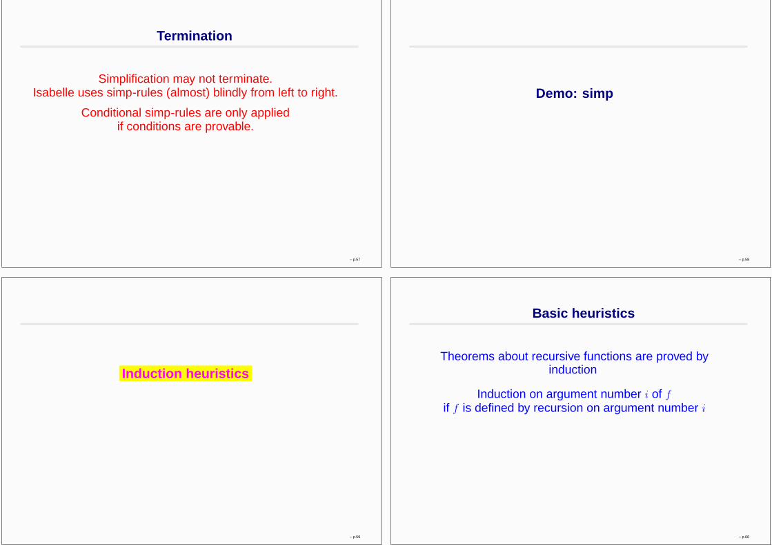
Termination

Simplification may not terminate.Isabelle uses simp-rules (almost) blindly from left to right.

Conditional simp-rules are only appliedif conditions are provable.

– p.57

Demo: simp

– p.58

Induction heuristics

– p.59

Basic heuristics

Theorems about recursive functions are proved byinduction

Induction on argument number i of f

if f is defined by recursion on argument number i

– p.60

A tail recursive reverse

consts itrev :: ’a list ⇒ ’a list ⇒ ’a listprimrec

itrev [] ys = ysitrev (x#xs) ys = itrev xs (x#ys)

lemma itrev xs [] = rev xs

Why in this direction?

Because the lhs is “more complex” than the rhs.

– p.61

Demo: first proof attempt

– p.62

Generalisation (1)

Replace constants by variables

lemma itrev xs ys = rev xs @ ys

– p.63

Demo: second proof attempt

– p.64

Generalisation (2)

Quantify free variables by ∀(except the induction variable)

lemma ∀ ys. itrev xs ys = rev xs @ ys

– p.65

HOL: Propositional Logic

– p.66

Overview

• Natural deduction• Rule application in Isabelle/HOL

– p.67

Rule notation

A1 . . . An

A instead of [[A1 . . . An]] =⇒ A

– p.68

Natural Deduction

– p.69

Natural deduction

Two kinds of rules for each logical operator ⊕:

Introduction: how can I prove A ⊕ B?

Elimination: what can I prove from A ⊕ B?

– p.70

Natural deduction for propositional logic

A BA ∧ B

conjIA ∧ B [[A;B]] =⇒ C

CconjE

AA ∨ B

BA ∨ B

disjI1/2 A ∨ B A =⇒ C B =⇒ CC

disjE

A =⇒ BA −→ B

impI A −→ B A B =⇒ CC

impE

A =⇒ B B =⇒ AA = B iffI A=B

A =⇒ B iffD1 A=BB =⇒ A iffD2

A =⇒ False¬ A

notI ¬ A AC

notE

– p.71

Operational reading

A1 . . . An

A

Introduction rule:To prove A it suffices to prove A1 . . . An.

Elimination ruleIf I know A1 and want to prove A

it suffices to prove A2 . . . An.

– p.72

Classical contradiction rules

¬ A =⇒ FalseA

ccontr ¬ A =⇒ AA classical

– p.73

Proof by assumption

A1 . . . An

Aiassumption

– p.74

Rule application: the rough idea

Applying rule [[ A1; . . . ; An ]] =⇒ A to subgoal C:• Unify A and C• Replace C with n new subgoals A1 . . . An

Working backwards, like in Prolog!

Example: rule: [[?P; ?Q]] =⇒ ?P ∧ ?Qsubgoal: 1. A ∧ B

Result: 1. A2. B

– p.75

Rule application: the details

Rule: [[ A1; . . . ; An ]] =⇒ ASubgoal: 1. [[ B1; . . . ; Bm ]] =⇒ C

Substitution: σ(A) ≡ σ(C)New subgoals: 1. σ( [[ B1; . . . ; Bm ]] =⇒ A1)

...n. σ( [[ B1; . . . ; Bm ]] =⇒ An)

Command:

apply(rule <rulename>)

– p.76

Proof by assumption

apply assumptionproves

1. [[ B1; . . . ; Bm ]] =⇒ C

by unifying C with one of the Bi (backtracking!)

– p.77

Demo: application of introduction rule

– p.78

Applying elimination rules

apply(erule <elim-rule>)

Like rule but also• unifies first premise of rule with an assumption• eliminates that assumption

Example:Rule: [[?P ∧ ?Q; [[?P; ?Q]] =⇒ ?R]] =⇒ ?R

Subgoal: 1. [[ X; A ∧ B; Y ]] =⇒ ZUnification: ?P ∧ ?Q ≡ A ∧ B and ?R ≡ Z

New subgoal: 1. [[ X; Y ]] =⇒ [[ A; B ]] =⇒ Zsame as: 1. [[ X; Y; A; B ]] =⇒ Z

– p.79

How to prove it by natural deduction

• Intro rules decompose formulae to the right of =⇒.

apply(rule <intro-rule>)• Elim rules decompose formulae on the left of =⇒.

apply(erule <elim-rule>)

– p.80

Demo: examples

– p.81

=⇒ vs −→

• Write theorems as [[A1; . . . ; An]] =⇒ Anot as A1 ∧ . . . ∧ An −→ A (to ease application)

• Exception (in apply-style): induction variable must notoccur in the premises.

Example: [[A; B(x) ]] =⇒ C(x) ; A =⇒ B(x) −→ C(x)

Reverse transformation (after proof):lemma abc[rule_format] : A =⇒ B(x) −→ C(x)

– p.82

Demo: further techniques

– p.83

HOL: Predicate Logic

– p.84

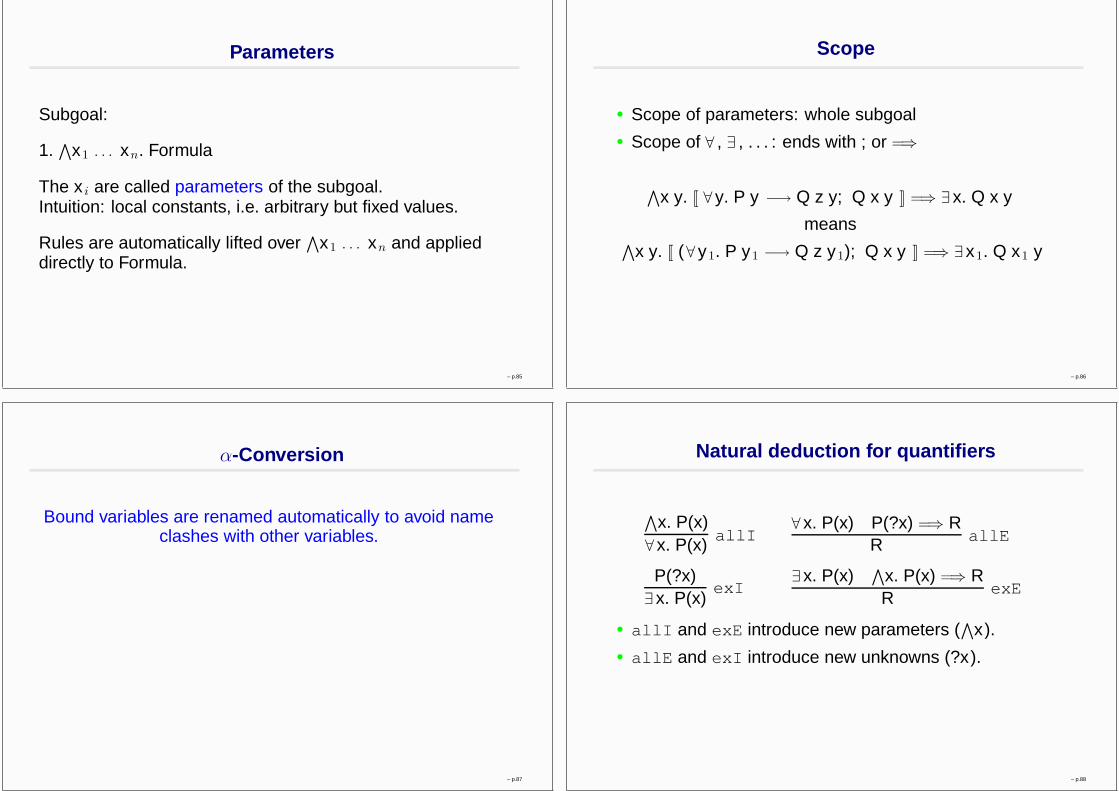
Parameters

Subgoal:

1.∧

x1 . . . xn. Formula

The x i are called parameters of the subgoal.Intuition: local constants, i.e. arbitrary but fixed values.

Rules are automatically lifted over∧

x1 . . . xn and applieddirectly to Formula.

– p.85

Scope

• Scope of parameters: whole subgoal• Scope of ∀ , ∃ , . . . : ends with ; or =⇒

∧x y. [[ ∀ y. P y −→ Q z y; Q x y ]] =⇒ ∃ x. Q x y

means∧

x y. [[ (∀ y1. P y1 −→ Q z y1); Q x y ]] =⇒ ∃ x1. Q x1 y

– p.86

α-Conversion

Bound variables are renamed automatically to avoid nameclashes with other variables.

– p.87

Natural deduction for quantifiers

∧x. P(x)

∀ x. P(x)allI

∀ x. P(x) P(?x) =⇒ RR allE

P(?x)∃ x. P(x)

exI∃ x. P(x)

∧x. P(x) =⇒ RR

exE

• allI and exE introduce new parameters (∧

x).• allE and exI introduce new unknowns (?x).

– p.88

Instantiating rules

apply(rule_tac x = "term" in rule)

Like rule, but ?x in rule is instantiated by term beforeapplication.

Similar: erule_tac

! x is in rule, not in the goal !

– p.89

Two successful proofs

1. ∀ x. ∃ y. x = yapply(rule allI)

1.∧

x. ∃ y. x = ybest practice explorationapply(rule_tac x = "x" in exI) apply(rule exI)1.

∧x. x = x 1.

∧x. x = ?y x

apply(rule refl) apply(rule refl)?y 7→ λu. u

simpler & clearer shorter & trickier

– p.90

Demo: quantifier proofs

– p.91

Safe and unsafe rules

Safe allI, exE

Unsafe allE, exI

Create parameters first, unknowns later

– p.92

Demo: proof methods

– p.93

Sets

– p.94

Overview

• Set notation• Inductively defined sets

– p.95

Set notation

– p.96

Sets

Type ’a set : sets over type ’a

• {}, {e1,. . . ,en}, {x. P x}• e ∈ A, A ⊆ B• A ∪ B, A ∩ B, A - B, - A•

⋃x∈A B x,

⋂x∈A B x

• {i..j}• insert :: ’a ⇒ ’a set ⇒ ’a set• . . .

– p.97

Proofs about sets

Natural deduction proofs:• equalityI: [[A ⊆ B; B ⊆ A]] =⇒ A = B• subsetI: (

∧x. x ∈ A =⇒ x ∈ B) =⇒ A ⊆ B

• . . . (see Tutorial)

– p.98

Demo: proofs about sets

– p.99

Inductively defined sets

– p.100

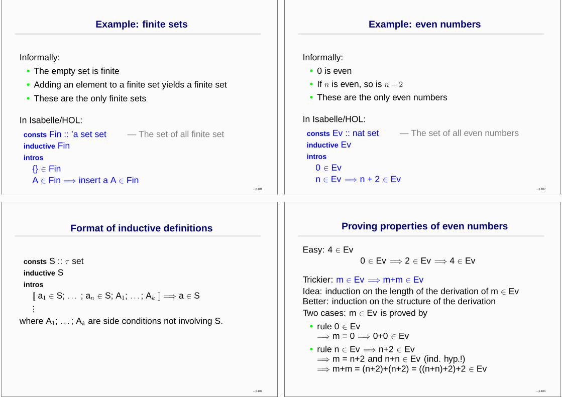
Example: finite sets

Informally:• The empty set is finite• Adding an element to a finite set yields a finite set• These are the only finite sets

In Isabelle/HOL:

consts Fin :: ’a set set — The set of all finite setinductive Finintros

{} ∈ FinA ∈ Fin =⇒ insert a A ∈ Fin

– p.101

Example: even numbers

Informally:• 0 is even• If n is even, so is n + 2

• These are the only even numbers

In Isabelle/HOL:

consts Ev :: nat set — The set of all even numbersinductive Evintros

0 ∈ Evn ∈ Ev =⇒ n + 2 ∈ Ev

– p.102

Format of inductive definitions

consts S :: τ setinductive Sintros

[[ a1 ∈ S; . . . ; an ∈ S; A1; . . . ; Ak ]] =⇒ a ∈ S...

where A1; . . . ; Ak are side conditions not involving S.

– p.103

Proving properties of even numbers

Easy: 4 ∈ Ev0 ∈ Ev =⇒ 2 ∈ Ev =⇒ 4 ∈ Ev

Trickier: m ∈ Ev =⇒ m+m ∈ EvIdea: induction on the length of the derivation of m ∈ EvBetter: induction on the structure of the derivationTwo cases: m ∈ Ev is proved by• rule 0 ∈ Ev

=⇒ m = 0 =⇒ 0+0 ∈ Ev• rule n ∈ Ev =⇒ n+2 ∈ Ev

=⇒ m = n+2 and n+n ∈ Ev (ind. hyp.!)=⇒ m+m = (n+2)+(n+2) = ((n+n)+2)+2 ∈ Ev

– p.104

Rule induction for Ev

To prove

n ∈ Ev =⇒ P n

by rule induction on n ∈ Ev we must prove• P 0• P n =⇒ P(n+2)

Rule Ev.induct:

[[ n ∈ Ev; P 0;∧

n. P n =⇒ P(n+2) ]] =⇒ P n

An elimination rule

– p.105

Rule induction in general

Set S is defined inductively.To prove

x ∈ S =⇒ P x

by rule induction on x ∈ Swe must prove for every rule

[[ a1 ∈ S; . . . ; an ∈ S ]] =⇒ a ∈ Sthat P is preserved:

[[ P a1; . . . ; P an ]] =⇒ P a

In Isabelle/HOL:apply(erule S.induct)

– p.106

Demo: inductively defined sets

– p.107