DI

SC

US

SI

ON

P

AP

ER

S

ER

IE

S

Forschungsinstitut zur Zukunft der ArbeitInstitute for the Study of Labor

Is Universal Child Care Leveling the Playing Field? Evidence from Non-Linear Difference-in-Differences

IZA DP No. 4978

May 2010

Tarjei HavnesMagne Mogstad

Is Universal Child Care Leveling the

Playing Field? Evidence from Non-Linear Difference-in-Differences

Tarjei Havnes ESOP, University of Oslo

Magne Mogstad

Statistics Norway, ESOP and IZA

Discussion Paper No. 4978 May 2010

IZA

P.O. Box 7240 53072 Bonn

Germany

Phone: +49-228-3894-0 Fax: +49-228-3894-180

E-mail: iza@iza.org

Any opinions expressed here are those of the author(s) and not those of IZA. Research published in this series may include views on policy, but the institute itself takes no institutional policy positions. The Institute for the Study of Labor (IZA) in Bonn is a local and virtual international research center and a place of communication between science, politics and business. IZA is an independent nonprofit organization supported by Deutsche Post Foundation. The center is associated with the University of Bonn and offers a stimulating research environment through its international network, workshops and conferences, data service, project support, research visits and doctoral program. IZA engages in (i) original and internationally competitive research in all fields of labor economics, (ii) development of policy concepts, and (iii) dissemination of research results and concepts to the interested public. IZA Discussion Papers often represent preliminary work and are circulated to encourage discussion. Citation of such a paper should account for its provisional character. A revised version may be available directly from the author.

IZA Discussion Paper No. 4978 May 2010

ABSTRACT

Is Universal Child Care Leveling the Playing Field? Evidence from Non-Linear Difference-in-Differences*

Advocates of a universal child care system offer a two-fold argument: Child care facilitates children’s long-run development, and levels the playing field by benefiting in particular disadvantaged children. Therefore, a critical element in evaluating universal child care systems is to measure the impact on child development in a way that allows the effects to vary systematically over the outcome distribution. Using non-linear DD methods, we investigate how the introduction of large-scale, publicly subsidized child care in Norway affected the earnings distribution of exposed children as adults. We find that mean impacts miss a lot: While child care had a small and insignificant mean impact, effects were positive over the bulk of the earnings distribution, and sizable below the median. This is an important observation since previous empirical studies of universal child care have focused on mean impacts. We further demonstrate that the essential features of our empirical findings could not have been revealed using mean impact analysis on typically defined subgroups. This is because the intragroup variation in the child care effects is relatively large compared to the intergroup variation in mean impacts. JEL Classification: J13, H40, I28, D31 Keywords: universal child care, child development, non-linear difference-in-differences,

heterogeneity, distributional effects Corresponding author: Magne Mogstad Research Department Statistics Norway P.O. Box 8131 Dep. N-0033 Oslo Norway E-mail: magne.mogstad@ssb.no

* Thanks to Rolf Aaberge, Erling Barth, Nabanita Datta Gupta, Halvor Mehlum, Hilary Hoynes, Kalle Moene, Mari Rege and Kjetil Telle, as well as participants at a number of seminars and conferences for useful comments and suggestions. Financial support from the Norwegian Research Council (194347/S20) is gratefully acknowledged. The project is also part of the research activities at the ESOP center at the Department of Economics, University of Oslo. ESOP is supported by The Research Council of Norway.

1 Introduction

The increased demand for child care associated with the rise of maternal employment isattracting the attention of policy makers and researchers alike. Indeed, access to childcare has gone up in many developed countries over the last years (OECD, 2004), and thereis a heated debate about a move towards subsidized, universally accessible child care orpre-school, as offered in the Scandinavian countries. For example, the European Union’sPresidency formulated in 2002 as a policy goal “to provide childcare by 2010 to at least90% of children between 3 years old and the mandatory school age and at least 33% ofchildren under 3 years of age” (EU, 2002, p. 13). In the US, the so-called ’Zero to FivePlan’ of US President Obama aims at making states move towards voluntary universalpreschool. Advocates of such a universal child care system argue that it is important infacilitating children’s long-run development. Moreover, it is claimed to be leveling theplaying field by benefiting especially disadvantaged children (see e.g. Karoly et al. 2005).Therefore, a critical element in evaluating universal child care systems is to measure theimpact on children’s outcomes in a way that allows for heterogeneous treatment effects.That is the focus of this study.

In this paper, we provide first evidence on the distributional effects of universal childcare on children’s outcomes. As in Baker et al. (2008) and Havnes and Mogstad (2009),universal child care is taken to mean large-scale, publicly subsidized child care arrange-ments open for everyone; not that all children were in fact using child care. Specifically,we analyze how a Norwegian child care reform from late 1975 affected the earnings dis-tribution of exposed children as adults. The reform assigned responsibility for child careto local governments and increased federal subsidies, which immediately generated largevariation in child care coverage for children 3–6 years old, both across time and betweenmunicipalities.1 As discussed below, formal child care both before the reform period andduring the expansion was severely rationed, with informal care arrangements (such asfriends, relatives, and unlicensed care givers) servicing the excess demand. In our analy-sis, we will focus on years immediately after the reform, when child care coverage increasedfrom 10 to 28 percent, most likely reflecting an abrupt slackening of constraints on thesupply side, rather than a spike in the local demand.

Our empirical analysis utilizes high-quality panel data from administrative registerscovering the entire resident population and all licensed care givers in Norway. To identifythe child care effects, we exploit that the supply shocks to formal care were larger insome areas than others. Specifically, we use standard (DD) methods to estimate meanimpacts, comparing the adult earnings for 3 to 6 year olds before and after the reform,from municipalities where child care expanded a lot (i.e. the treatment group) and munic-

1Throughout this paper, child care coverage rates refer to formal care, including publicly and privatelyprovided child care institutions as well as licensed care givers, all eligible to subsidies from the government.

1

ipalities with little or no increase in child care coverage (i.e. the comparison group). In asimilar vein, we use non-linear DD methods to map out the child care effects on the entireearnings distribution of exposed children as adults. This allows us to move beyond meanimpacts, examining whether the effect of child care is constant across the distribution, orwhether it leads to larger changes in certain parts of the distribution.

In our empirical analysis, we use two different non-linear DD methods. First, wetake the method proposed by Firpo et al. (2009) for estimating unconditional quantiletreatment effects (under the conditional independence assumption) to a DD framework,controlling also for unobserved time and group effects. Their method turns the difficultestimation problem of estimating the treatment effect on unconditional quantiles of theoutcome distribution, into the simple estimation problem of estimating the treatmenteffect on the probability of being above a certain threshold of the outcome distribution.We further provide empirical results using an alternative approach to analyze the distri-butional effects of policy changes within a DD framework: the quantile DD model.2 Bothmethods estimate the counterfactual distribution, which we use to map out the child careeffects on the long-run earnings distribution of the children. It’s heartening to find thateven though the identifying assumptions are different, the results are quite similar. Tofurther increase the confidence in our empirical strategies, we run a battery of specificationchecks.

The insights from our empirical results may be summarized with three conclusions.First, mean impacts miss a lot, concealing major heterogeneity: While child care had asmall and insignificant mean impact, effects were positive over the bulk of the earningsdistribution, and sizable below the median. This is an important observation since previ-ous empirical studies of universal child care have focused on mean impacts.3 Second, theestimated heterogeneity in child care effects is consistent with predictions from economictheory. In particular, formal child care is predicted to reduce the importance of familybackground for child development by serving as a substitute for parental care or informalcare arrangements, in end effect leveling the playing field. Third, the essential featuresof our empirical findings could not have been revealed using mean impact analysis ontypically defined subgroups. This is because the intragroup variation in the child careeffects is relatively large compared to the intergroup variation in mean impacts.4

In sum, our study shows that non-linear DD methods can play a useful role in as-sessing policy changes, when only non-experimental data is available and theory predictsheterogeneous treatment effects. Our analysis also serves as an example of how the pivotalargument in favor of universal child care might not be that it, on average, improves the

2See Athey and Imbens (2006) for a detailed discussion of the quantile DD method, and Poterba etal. (1995) and Meyer et al. (1995) for applications.

3For a recent review, see Almond and Currie (2010).4This finding echoes the conclusion drawn in Bitler et al. (2006), who evaluate the labor supply

responses to the Jobs First welfare reform.

2

long-run prospects of children, but rather that it levels the playing field.This paper proceeds as follows. Section 2 discusses our study in relation to previous

research on child care and child development. Section 3 describes the 1975 child carereform and the succeeding expansion in child care, before outlining a parsimonious the-oretical framework making predictions about the effects of the policy changes on childdevelopment. Section 4 outlines the empirical strategy and Section 5 presents our data.Section 6 presents the main empirical findings, and reports results from specificationchecks. Section 7 concludes with a discussion of policy implications.

2 Child care and child development

Recent research from a number of fields suggests that investments in early childhood havehigh returns, especially for disadvantaged children (Knudsen et al., 2006). Studies in neu-roscience and development psychology indicate that learning is easier in early childhoodthan later in life (Shonkoff and Phillips, 2000). In the economics literature, Becker (1964)points out that the returns to investments in early childhood are likely to be relativelyhigh, simply because of the long time to reap the rewards. Taking this argument onestep further, Carneiro and Heckman (2004) argue that investments in human capital havedynamic complementarities, implying that learning begets learning.

On this background, Currie (2001) suggests that governments should aim to equalizeinitial endowments through early childhood development, rather than compensate for dif-ferences in outcomes later in life. The role of governments in facilitating child developmentis particularly important, both from positions on equity and efficiency, if families under-invest in early childhood due to market failures such as liquidity constraints, informationfailures, and externalities (Gaviria, 2002).

Child care institutions are important arenas for child development, and expandingchild care coverage is an explicit goal in many countries. This has been motivated byevidence showing that early childhood educational programs can generate learning gainsin the short-run and, in many cases, improve the long-run prospects of children from poorfamilies.5 While the results from these studies are encouraging, the programs evaluatedwere unusually intensive and involved small numbers of particularly disadvantaged chil-dren from a few cities in the US. A major concern is therefore that this evidence may tellus little about the effects of universal child care systems offered to the entire population(Baker et al., 2008). Nonetheless, it has fuelled an increasing interest in universal pro-vision of child care as a means of advancing child development and improving children’slong-run outcomes.

5The Perry Preschool and Abecedarian programs are commonly cited examples of how high-qualitypreschool services can improve the lives of disadvantaged children. See Barnett (1995) and Karoly et al.(2005) for surveys of the literature.

3

Our paper contributes to a small but rapidly growing literature on the effects ofuniversal child care programs. Almost all the evidence is limited to short-run outcomesand the findings are mixed. Loeb et al. (2007), for instance, find that pre-primaryeducation in the US is associated with improved reading and mathematics skills at primaryschool entry. However, Magnuson et al. (2007) suggest that these effects dissipate for mostchildren by the end of first grade. Positive effects of child care on children’s short-runoutcomes are also found by Gormley and Gayer (2005), Fitzpatrick (2008), Melhuish et al.(2008), and Berlinski et al. (2008, 2009). On the other hand, Baker et al. (2008) analyzethe introduction of subsidized, universally accessible child care in Quebec, finding noimpact on children’s short-run cognitive skills but substantial negative effects on children’sshort-run non-cognitive development. These negative effects echo the results in Herbst andTekin (2008), while Datta Gupta and Simonsen (2007) find that compared to home care,being enrolled in preschool does not lead to significant difference in child non-cognitiveoutcomes.

While the evidence on short-run effects of universal child care programs is of interest,a crucial question is whether these effects persist, and perhaps are amplified, over time.As noted by Baker et al. (2008), negative short-run effects could reflect that children havedifficulties in their first interactions with other children. In that case, child care attendancemay expose children to these costs earlier on, so that they are better prepared for attendingschool. In addition, evidence from early intervention programs targeting particularlydisadvantaged children suggests that even though the short-run gains in test-scores tendedto dissipate over time, there were strong and persistent impacts on long-run outcomes(Heckman et al., 2006). Havnes and Mogstad (2009) and Cascio (2009) circumvent theseissues by investigating the impact of universal child care on adult outcomes that are ofintrinsic importance. In doing so, they also avoid reliance on test scores and changes intest scores that have no meaningful cardinal scale (see Cunha and Heckman, 2008).

Havnes and Mogstad (2009) find that universal child care in Norway had strong pos-itive impacts on children’s educational attainment and labor market participation asadults. Their subsample analysis indicates that girls and children with low educatedparents benefit the most from child care. In terms of mechanisms, they find that the in-crease in formal child care largely displaced informal care, without much effect on mother’slabor force participation. Cascio (2009) uses data from four decennial censuses to analyzethe introduction of public preschools in the US. Using a cohort-based design, her base-line specification suggests that white children born after the reform in states that beganfunding kindergartens, largely in the South, were less likely to drop out of high-school.Yet she finds no effect on several other outcomes, like employment, college attendance,and earnings. Nor does she find any effects for blacks. She interprets the general lack ofprogram effects as a result of (i) the low-intensity nature of the program, (ii) significantcrowding out of participation in federally-funded programs, such as Head Start, and (iii)

4

cut-backs in state expenditure on schools to fund kindergartens.However, the policy debate on universal child care policies is not restricted to whether

child care, on average, improves child development: Distributional considerations alsocome to play. As emphasized by Almond and Currie (2010), formal child care is likely toreduce the importance of family background for child development by serving as a sub-stitute for parental care or informal care arrangements, in end effect leveling the playingfield. A concern is therefore that the estimated mean impacts may average together ef-fects of different sign and magnitude, possibly obscuring the extent of child care’s effects.The focus of our study is to address this concern. Specifically, we follow Havnes andMogstad (2009) in considering a Norwegian child care reform from late 1975, introducingsubsidized, universally accessible child care. We also use the same data, administrativeregisters covering the entire population. Our point of departure is to use non-linear DDmethods to map out the child care effects on the entire earnings distribution of exposedchildren as adults, rather than using a standard DD approach to estimate mean impactslike previous studies.

3 Background and Theoretical Framework

In this section, we describe the Norwegian child care system before and after the 1975reform,6 before outlining a parsimonious theoretical framework making predictions aboutthe effects of the policy changes on child development.

The child care reform. In the post-WWII years in Norway, the gradual entry on thelabor market of particularly married women with children, caused growing demand forout-of-home child care. In a survey from 1968, when child care coverage was less thanfive percent, about 35% of mothers with 3 to 6 year olds stated demand for formal childcare (NOU, 1972). In the same survey, only 34% of the latter group of respondents statedthat they were in fact using out-of-home child care on a regular basis. Out of these, just14 percent were in formal child care, while more than 85 percent were using informalarrangements.7

The severe rationing of formal child care acted as a background for political progresstowards public funding of child care.8 In the early 1950s, grants and subsidized loans weretemporarily made available for construction and refurbishment of child care institutions,and their operation was regulated by law in 1954. Federal subsidies to formal child

6The description of the reform draws heavily on Havnes and Mogstad (2009). See also Leira (1992,ch. 4) for a detailed survey of the history of Norwegian child care policies since WWII.

7Relatives stand out as the largest group of informal care givers at 35 percent, followed by play parksat 20 percent, maids at 14 percent, other unlicensed care givers at 10 percent, and finally more irregulararrangements (such as neighbors and friends) at 7 percent (NOU, 1972).

8See Leira (1992, ch. 4) and The Norwegian Ministry of Children and Family Affairs (1998) for detailedsurveys of the history of Norwegian child care policies since WWII.

5

care were assigned a permanent post on the national budget in 1962, and increased overthe subsequent ten years from a modest USD 50 per child care place to a maximum ofmore than USD 1,200 annually.9 The child care subsidies were contingent on a federallydetermined maximum price to be paid by the parents, which in 1972 was about USD 215per month for full time care (NOU, 1972).

In 1972, the Norwegian government presented the Kindergarten White Paper (NOU,1972), proposing radical changes in public child care policies. To (i) create positive arenasfor child development, (ii) free labor market reserves among mothers, and (iii) lessen theburden on parents and relieve stress in the home, it was argued that child care shouldbe made universally available. This marked a strong shift in child care policies, fromfocusing on children with special needs (in particular disabled children and children fromdisadvantaged families) to a focus on a child care system open to everyone.

In June 1975, The Kindergarten Act was passed by the Norwegian parliament withbroad bipartisan political support. It assigned the responsibility for child care to localmunicipalities, but included federal provisions on educational content, group size, staffskill composition, and physical environment. By increasing the level of federal subsidiesfor both running costs in general and investment costs for newly established institutions,the government aimed at quadrupling the number of child care places to reach a total of100,000 by 1981.10

In the years following the reform, the child care expansion was progressively rolledout at a strong pace, with federal funding more than doubling from USD 34.9 millionin 1975 to 85.8 million in 1976, before reaching 107.3 million in 1977.11 This impliedan increase in the federal coverage of running costs from about 10% in 1973 to 17,6% in1976, and further to 30% in 1977. From 1976, newly established child care places receivedadditional federal funds for a period of five years. Municipalities with relatively low childcare coverage rates were awarded 60% more subsidies, whereas other municipalities wereawarded 40% extra.

Altogether, the reform constituted a substantial positive shock to the supply of formalchild care, which had been severely constrained by limited public funds. In succeedingyears, the previously slow expansion in subsidized child care accelerated rapidly. Froma total coverage rate of less than 10% for 3 to 6 year olds in 1975, coverage had shotup above 28% by 1979. Over the period, a total of almost 38,000 child care places wereestablished, more than a doubling from the 1975-level. By contrast, there was almost nochild care coverage for 1 and 2 year olds during this period. Figure 1 draws child care

9Throughout this paper, all monetary figures are fixed at 2006-level. For the figures expressed in USdollars, we have used the following exchange rate: NOK/USD = 6.5.

10In addition, the price-setting was delegated to local municipalities, abolishing the federally determinedmaximum parental price for child care subsidies. However, Gulbrandsen et al. (1981) report survey datasuggesting that the maximum price to be paid by the parents actually changed little in the years followingthe reform, and formal child care remained rationed well into the 90s

11Source: National budgets 1975/76 through 1978/79.

6

Figure 1: Child care coverage rate in Norway 1960–1996 for children 3–6 years old.Sources: Administrative data for 1972–1996. Data for 1960–1972 from NOU (1972), Table II.1.

coverage rates in Norway from 1960 to 1996 for 3 to 6 year olds. As is apparent from thefigure, there has been strong growth in child care coverage rates since 1975, particularlyin the early years. In our analysis, we will focus on the early expansion, which likelyreflects an abrupt slackening of constraints on the supply side, rather than a spike in thelocal demand.

We might worry about confounding the estimated child care effects with other reformsor changes taking place in the same period. However, we have found no significant reformsor breaks in trends that could be of concern for our estimations. An extension in ma-ternity leave implemented in 1977 did not affect the children in our sample directly, butcould potentially influence family size, which could in turn matter for child development.However, the reform was nationwide, and should be controlled for by cohort fixed-effects.In addition, our rich set of controls may pick up potentially remaining effects of this pol-icy change. Importantly, there were no significant changes in the Norwegian educationalpolicies affecting the cohorts of children we consider. On the contrary, Norway was knownfor its unified public school system based on a common national curriculum, rooted ina principle of equal rights to high-quality education, regardless of social and economicbackground or residency. This is mirrored in very similar expenditure levels per studentacross municipalities and virtually no private schools.12

The Organization of Formal Child Care. To interpret our results, we must understandthe type of care we are studying. The Ministry of Consumer Affairs and Administrationwas responsible for overall regulation of formal child care. Specifically, the Kindergarten

12See Telhaug et al. (2006), Volckmar (2008), and Havnes and Mogstad (2009) for an in-depth discus-sion of the Norwegian educational system relevant for the cohorts of children we consider.

7

Act regulated the authorisation, operation and supervision of formal child care institu-tions. The act defined formal child care institutions as care and educationally orientedenterprises for pre-school children, where an educated preschool teacher was responsiblefor the education. Formal child care institutions were run either by the municipalities orby firms, public institutions or private organisations, under the approval and monitoringof local authorities in the municipality. Table 1 reports child care institutions by ownerbiannually from 1975 through 1981, and shows the strong growth in municipal and coop-erative child care centers. Over the period, the share of private centers decreased from 28to 22 percent, driven almost entirely by a decline in the share of centers run by privateorganizations.

Regardless of ownership, formal child care institutions were required to satisfy federalprovisions on educational content and activities, group size, staff skill composition andphysical environment. The Kindergarten Act specified regulations, and guidelines wereformulated for activities and content. To be eligible for subsidies, institutions were obligedto meet the requirements and follow the guidelines. To secure opportunities for parentalinvolvement and promote cooperation between staff and parents, the Kindergarten Actrequired that every institution must have a parent council and a coordinating commit-tee. Local authorities were required by law to monitor the fulfillment of these federalprovisions.

As discussed above, formal child care institutions were financed jointly by the federalgovernment, municipalities and parents. All approved institutions received subsidies forrunning and establishment costs from the federal government. Subsidies were determinedon the basis of the number and age of children, and the amount of time they spent in formalchild care. In general, formal child care institutions were open during normal workinghours. All children were eligible, and open slots were in general allocated according tolength of time on the waiting list and age. Only under special circumstances could a childgain priority on the waiting list.

Table 1: Child care institutions by ownership structure

1975 1977 1979 1981Private (%) 28.4 26.7 26.3 21.9Municipality (%) 48.6 45.4 46.9 51.2Church (%) 7.3 8.0 8.6 8.6Cooperatives (%) 5.6 8.2 9.7 10.0

No. of child care institutions 880 1,469 2,294 2,754No. of children in child care (3–6 y.o.) 25,536 43,239 63,218 73,152Coverage rate (3–6 y.o., %) 10.0 17.6 28.1 34.2Notes: Private ownership indicates ownership by a private firm, organisation or foundation. Cooper-atives are parental or residential. Categories not reported are ownership by state, regions and other.

8

Every formal child care institution had to be run by an educated pre-school teacherresponsible for day-to-day management. The pre-school teacher education is a collegedegree, including supervised practice in a formal child care institution. Through hisor her position and training, this head teacher was responsible for ensuring satisfactoryplanning, observation, collaboration and evaluation of the work. The head teacher wasalso in charge of staff guidance, as well as collaboration with parents and local authorities,such as health stations, child welfare services and educational/psychological services. Inaddition, formal child care institutions were required to have at least one educated pre-school teacher per 16 children aged 3–6. Teachers typically worked closely with one ortwo assistants, and were responsible for the educational programmes in separate groupsand for day-to-day interaction with parents. There were no educational requirements forassistants.

In terms of educational content, a social pedagogy tradition dominated the child carepractices, according to which children where supposed to develop social, language andphysical skills mainly through play and informal learning.13 The informal learning wastypically carried out in the context of day-to-day social interaction between children andstaff, in addition to specific activities for different age groups.

Overall, formal child care in Norway (along with other Nordic countries) was charac-terized by relatively high expenditure levels per child compared to large-scale programsin other countries. For example, the average yearly expenditure for a slot in formal childcare was approximately USD 6,600.14 This is, for instance, substantially higher thanthe expenditures for the Head Start Program in the US aimed at low-income families,which cost around USD 5,000 per year (Currie, 2001). The high expenditure levels weremirrored in fairly extensive requirements to qualifications of child care staff and physicalenvironment, as well as a relatively low number of children per staff. For example, theaverage staff–child ratio was about 1:8 in 1977. In comparison, in the US and Canada,the corresponding ratio is 1:12, in Spain 1:13, and France 1:19 (see Datta Gupta andSimonsen, 2007).

Theoretical framework. As discussed in Currie and Almond (2010), formal child care islikely to reduce the importance of family background for child development by servingas a substitute for parental care or informal care arrangements, in end effect levelingthe playing field. Specifically, our child care reform may be interpreted as a subsidy toparents for choosing out-of-home care of a particular quality, generating at least one and

13The social pedagogy tradition to early education has been especially influential in the Nordic coun-tries and Central-Europe. In contrast, a so-called pre-primary pedagogic approach to early educationhas dominated many English and French-speaking countries, favoring formal learning processes to meetexplicit standards for what children should know and be able to do before they start school.

14Estimated annual budgetary cost per child care place from NOU (1972) is about USD 5,400 per child3–6 years old. In addition, investment costs are estimated at about USD 12,000 per child care place,adding USD 1,200 to the annual cost if written down over ten years.

9

possibly two convex kinks in the family’s budget constraint. Figure 2 illustrates thispoint by drawing family budget frontiers between child quality and parental consumptionbefore and after the reform. The parents trade off their own consumption, c, and childquality, q, given their budget constraint. For instance, parents could invest in children bydecreasing labor supply, by paying for higher quality out-of-home care, or by purchasingchild goods. The budget frontier of feasible combinations of consumption and child qualitythen resembles a standard production possibilities frontier.15

In Panel (a) of Figure 2, subsidized child care is not available. Trading off child qualitywith their own consumption, parents optimize by choosing a point in the tangency ofan indifference curve and the budget frontier. Panel (b) and (c) draw two examples ofalternative budget frontiers (dotted curves), in a situation with subsidized child care. Thedecision to (apply for and) take up a child care place is discrete. In reality, parents couldtypically choose to pay for either a full or a half day of care. For simplicity, we assumefull discreteness where parents either use formal child care or they don’t. Because parentscould choose not to spend money on formal child care and get higher consumption, thefrontiers using formal child care will be below the frontier without formal child care atthe c-axis. Further, if parents choose to purchase formal child care, they must be betteroff. That is, for parent’s to accept the offer of subsidized formal care, the budget frontierswith formal child care must be outside the frontier without formal child care, generatingat least one convex kink where the latter curve is steeper than the former curve at thepoint of intersection. Introduction of formal child care must therefore have a positiveeffect on child quality around this point. This is illustrated in Panels (b) and (c): Parentswho were previously located in a point like A will now optimally locate in a point like A′,where child quality is higher. Their children will benefit from the reform, at a decreasingrate in their pre-reform q.

If the maximum feasible child quality is lower with formal child care than without,the two frontiers will intersect again, generating a second convex kink.16 However, in thiscase the frontier with formal child care will be steeper than the curve without formal childcare. The introduction of formal care will, therefore, have an unambiguously negativeeffect on child quality around this point. This is illustrated in Panel (b): Parents whowere previously located in a point like B will now optimally move to point B′, trading offchild quality for parental consumption. The reform will be detrimental for their children’squality, and at an increasing rate in their pre-reform q. In comparison, Panel (c) considers

15Formally, with fixed wages w and unit consumer prices and time endowment, the budget constraintis w(1 − h) ≤ c + p(q), where h is home care, and p(q) reflects the cost-minimizing price of providingchild quality q. With child quality produced from a standard child production function, p(q) should beincreasing and convex in quality.

16The existence of a second intersection depends on the possibility and efficiency of topping up formalcare investments with market goods or informal care. While using formal care should exclude additionalinvestments during a substantial portion of the day, suggesting lower maximal quality, parents can bethought to be somewhat richer since formal care is subsidized, pulling in the opposite direction.

10

(a) Pre-reform (b) Post-reform, Case I (c) Post-reform, Case II

Figure 2: Family budget frontiers between child quality and parental consumption beforeand after the reform.Notes: Panel (a) displays budget frontier without subsidized formal child care. Panels (a) and (b) displaybudget frontiers with and without subsidized formal child care. In the panel (b), the maximum feasiblechild quality is lower with formal child care than without. In the panel (a), the maximum feasible childquality is lower without formal child care than with.

a situation where the two budget frontiers do not intersect a second time. In this case, theoverall effect is ambiguous, and depends on parental preferences. Specifically, the reformeffect on children from families who were previously investing heavily in child quality,located in points like B, will be ambiguous and depend on income and substitution effects.Finally, parents that prior to the reform choose a q far left of A or far right of B will notbe affected by the child care reform, because they will not use any formal care offered.

In sum, the predicted effects on children’s outcome distribution of the child care reformare heterogeneous: There should be no change at the bottom, increases in the lower andmiddle parts, decreases at the upper part, and perhaps no change at the very top. Insuch a situation, the mean impact would average together effects of different sign andmagnitude across the distribution, possibly obscuring the extent of child care’s effects.

4 Empirical strategy

To estimate the effects of universal child care on children’s earnings as adults, we followthe previous literature closely in using a DD framework. In particular, our identificationexploits that the supply shocks to formal child care were larger in some areas than others.Below, we describe our treatment definition, before specifying our standard and non-linearDD approaches. As always in policy evaluation using non-experimental data we cannotcompletely guard against such omitted variables bias. Yet to increase the confidence inour identification strategies, we run a battery of specification checks which are discussedafter the main results, in Section 6.

Treatment definition. Our main empirical strategy is the following: We compare adultearnings for children who were 3 to 6 year olds before and after the reform, from munic-ipalities where child care expanded a lot (i.e. the treatment group) and municipalities

11

Figure 3: Child care coverage rates 1972–1985 for 3–6 year olds in treatment and com-parison municipalitiesNotes: Treatment (comparison) municipalities are above (below) the median in child care coverage growthfrom 1976 to 1979.

with little or no increase in child care coverage (i.e. the comparison group).The child care expansion started in 1976, affecting the post-reform cohorts born 1973–

1976 with full force, and to a lesser extent the phase-in cohorts born 1970–1972. Thepre-reform cohorts consist of children born in the period 1967–1969. We consider theperiod 1976–1979 as the child care expansion period. In the robustness analysis, we takeseveral steps to ensure that our results are robust to the exact child care coverage cut-off,defining treatment and comparison groups.

To define the treatment and comparison group, we order the municipalities accordingto the percentage point increase in child care coverage rates from 1976 to 1979. Wethen separate the sample at the median, letting the upper half constitute the treatmentmunicipalities and the lower half the comparison municipalities. Figure 3 displays childcare coverage before and after the 1975 reform in treatment and comparison municipalities(weighted by population size). The graphs move almost in parallel before the reform, whilethe child care coverage of the treatment municipalities kinks heavily after the reform. Thisillustrates that our study compares municipalities that differ distinctly in terms of changesin child care coverage within a narrow time frame. In the robustness analysis, we considerwhether variations in treatment intensity affects our results, by changing the child carecoverage cut-off defining the treatment and comparison municipalities.

12

4.1 Mean impact estimation

When estimating mean impacts in the population of children as a whole and in subgroupsby child and parental characteristics, we use the same DD specification as Havnes andMogstad (2009). Our baseline regression model, estimated by OLS over the sample ofchildren born during the period 1967–1976, can be defined as

Yijt = ψt + γ1Treati + γ2(Treati × Phaseint) + θ(Treati × Postt) +X ′ijtβ + ϵijt, (1)

where Y is the earnings in 2006, i indexes child, j indexes family, and t indexes the year thechild turns 3 years old. The vector of covariates X includes parental age, their educationwhen the child is 2 years old, their age at first birth, the number of older siblings (also cap-turing birth order) and relocation between municipalities within treatment/comparisonarea, the child’s sex and immigrant status, as well as municipality-specific fixed effects.The error term ϵijt is clustered on the mother, allowing for dependence in the residualsof siblings.17 The dummy variable Treatedi is equal to 1 if child i lives in the treatmentarea, Phaseint and Postt are dummy variables equal to 1 when t ∈ [1973, 1975] andt ∈ [1976, 1979] respectively, while ψt are cohort-specific fixed effects.

The parameter of interest, θ, captures the average effect on children who reside inthe treatment area in the post-reform period, of additional child care slots following thereform in the treatment municipalities compared to the comparison municipalities. Thereare two types of averaging underlying this average causal effect. First, there is averagingover the impacts on children from different municipalities in the treatment area. Andsecond, there is averaging across the marginal effects of the additional child care slots.

Like in Baker et al. (2008) and Havnes and Mogstad (2009), we will interpret θ asthe mean intention-to-treat effect (ITT), since our regression model estimates the reducedform impacts on all children from post-reform cohorts who reside in the treatment area.An advantage of the ITT parameter is that it captures the full reform impact of changesin both formal and informal care arrangements, as well as any peer effects on children whowere not attending child care. However, since this parameter averages the reform effectsover all children in the municipality, it reflects poorly the size of the child care expansion.To arrive at the treatment-on-the-treated (TT) effect, we follow Baker et al. and Havnesand Mogstad and scale the ITT parameter with the probability of treatment. Specifically,we divide the ITT parameter with the increase in child care coverage following the reformin the treatment group relative to the comparison group. For example, TT = ITT/0.1785in our baseline specification. The TT parameter gives us the effect of child care exposure –per child care place – on children born in post-reform cohorts who reside in the treatment

17Bertrand et al. (2004) show that the standard errors in DD regressions may suffer from serialcorrelation. As their analysis demonstrates, we reduce the problem of serial correlation considerably bycollapsing the time-series dimension into three periods: pre-reform, phase-in, and post-reform.

13

area. For ease of interpretation, we will throughout the paper report the TT parameters(and their standard errors).

4.2 Non-linear difference-in-differences estimation

To map out the child care effects on the earnings distribution of exposed children asadults, we use non-linear DD methods. Our main empirical strategy extends the methodproposed by Firpo et al. (2009) for estimating unconditional quantile treatment effects(under the conditional independence assumption) to a DD framework, controlling alsofor unobserved time and group effects. To define this threshold DD estimator, let Fgt

denote the earnings distribution in group g at time t, where g = 1 indicates the treatmentgroup (and g = 0 the comparison group) and t = 1 indicates the post-reform cohorts(and t = 0 pre-reform cohorts). The estimator (without covariates) for the counterfactualpost-reform distribution in the treatment group in the absence of the child care reform,F̃ T

11, can be defined as

F̃ T11(y) = F10(y) +

[F01(y) − F00(y)

].

The reform effect at a particular earnings level y, denoted τT (y), is then given by thedifference between the actual (observed) earnings distribution and the estimated counter-factual distribution at this point, that is τT (y) = F11(y) − F̃ T

11(y).Following Firpo et al. (2009), the analogous regression model with covariates can be

specificed as

Pr(Yijt ≥ y) = ψyt + γy

1Treati + γy2 (Treati × Phaseint) + θy(Treati × Postt) (2)

+X ′ijtβ

y + ϵyijt,

where X is the same set of controls as in the mean impact estimation. As shown by Firpoet al. (2009), this turns the difficult estimation problem of estimating the treatmenteffect on unconditional quantiles of the outcome distribution, into the easy estimationproblem of estimating the treatment effect on the probability of being above a certainthreshold of the outcome distribution. The reason is that, unlike the conditional quantile,the conditional mean averages up to the unconditional mean, due to the law of iteratedexpectations. As a result, the OLS estimate of θ in equation (2) gives the unconditionalreform impact on the probability of earning at least y.18 In our empirical analysis, weestimate the reform effects at the earnings levels of all percentiles 1-99 in the pre-reformdistribution in the treatment group.

18Our linear probability model will be the best least-squares approximation of the true conditionalexpectation function. As noted by Angrist (2001), if there are no covariates or they are discrete, as inour case, linear models are no less appropriate for limited dependent variables than for other types ofdependent variables.

14

To examine the robustness of our results, we also report estimation results from anothernon-linear DD approach, the quantile DD method which is described in detail in Atheyand Imbens (2006). As before, we estimate the counterfactual earnings distribution bytaking the observed distribution among pre-reform cohorts from the treatment groupand adjusting for the growth from pre-reform to post-reform cohorts in the earningsdistribution of the comparison group. However, we adjust by using the change in thequantiles, rather than the change in population shares as in the threshold DD estimator.Specifically, the quantile DD estimator (without covariates) for the counterfactual post-reform distribution in the treatment group in the absence of the reform, F̃Q

11, can bedefined as

F̃Q−111 (q) = F−1

10 (q) +[F−1

01 (q) − F−100 (q)

]The estimated reform effect at a particular quantile is then given analagously to the above,by τQ(q) = F−1

11 (q) − F̃Q−111 (q).

The two non-linear DD methods are similar, but rely on different dimensions of thedistributions in the identifying assumptions. To compare them more explicitly, Figure4 draws the observed earnings distributions in 2006 separately for pre- and post-reformcohorts from treatment and comparison municipalities. Since post-reform cohorts areyounger, it is not surprising that they have lower earnings than those from pre-reform co-horts. Further, it is evident that the pre-reform cohorts in the treatment and comparisongroups have very similar earnings, until about the 70th percentile. At higher percentiles,earnings levels in the treatment group are somewhat higher than in the comparison group.This suggests that a direct comparison of children from treatment and comparison munic-ipalities would be likely to overestimate the effect of the reform on these higher quantiles.The DD methods, however, achieve identification from the changes in these differences,so we are not concerned with differences between the treatment and comparison group inthe earnings levels as such.

15

Figu

re4:

Earn

ings

dist

ribut

ion

inpr

e-re

form

and

post

-ref

orm

coho

rts

intr

eatm

ent

and

com

paris

onm

unic

ipal

ities

(NO

K1,

000)

.N

otes

:Pr

e-re

form

coho

rtsa

rebo

rn19

67–1

969,

and

post

-ref

orm

coho

rtsa

rebo

rn19

73–1

976.

Trea

tmen

t(co

mpa

rison

)mun

icip

aliti

esar

eab

ove

(bel

ow)t

hem

edia

nin

child

care

cove

rage

grow

thfr

om19

76to

1979

.

16

With threshold DD, we compare the horizontal differences in Figure 4. Consider,for example, the earnings level at the pre-reform 90th percentile, Yq90. The thresholdDD estimator compares the difference in population shares below this level of earningsamong individuals from pre-reform cohorts, TDID0, with the corresponding differenceamong children from post-reform cohorts, TDID1. The reform effect at Yq90 is estimatedas TDID1 − TDID0. Holding the level of earnings fixed, our threshold DD compareschanges in the distributions around Yq90, that is, we compare the population shares withearnings below a certain threshold. The identifying assumption boils down to the earningsgrowth from pre-reform to post-reform cohorts around this particular earnings level beingthe same in the treatment group as in the comparison group, in the absence of the reform.

In contrast, the quantile DD holds the quantile fixed, and compares changes in thelevel of earnings around this quantile. Considering again the 90th percentile markedin the figure, the quantile approach considers the difference in earnings at this quan-tile among pre-reform cohorts, QDID0, and compares this to the difference in earningsamong post-reform cohorts at the same quantile, QDID1. The identifying assumptionis that the growth in earnings from pre-reform to post-reform cohorts at this particularquantile would have been the same in the treatment group as in the comparison group,in the absence of the reform. However, as is evident at the 90th percentile in Figure 4,the earnings levels at these quantiles may be quite different between the treatment andcomparison group. If the earnings levels at a given quantile differ between the treatmentand comparison group and the growth in earnings depends on the earnings levels, it islikely that the identifying assumption of the quantile DD model is violated. In our view,this makes the quantile DD estimator somewhat less attractive than the threshold DDestimator.

Another advantage of the threshold DD estimator is that it is straightforward tocontrol for differences between the treatment and comparison group in child and parentalcharacteristics. Unlike conditional means, conditional quantiles do no average up to theirunconditional counterparts. As a result, a conditional quantile regression cannot in generalbe used to identify the unconditional quantile treatment effects (see Firpo et al., 2009).To handle covariates in our quantile DD method, we therefore follow Firpo (2007) inusing an inverse propensity score re-weighting procedure, with weights determined by thepropensity for treatment depending on X. Appendix B describes our implementation ofthis procedure, and compares the results from the two non-linear DD methods, with andwithout covariates.

It should finally be noted that the non-linear DD methods identify the child care effecton the earnings distribution, which will, in general, differ from the distribution of childcare effects, unless the effects are rank-preserving (see Heckman et al. 1997). However,our focus is on the distributional effects of the child care reform: For this purposes, theeffect on the outcome distribution is what we are after. Also, any differences in the TT

17

parameters between subgroups and at different parts of the outcome distribution, may re-flect both differences in child care take-up and potentially heterogenous impacts of uptake,in line with the predictions from our theoretical framework. Adjusting for differences intake-up across the earnings distribution would require strong assumptions about how thechild care reform shifts the ranks of the children. Making such assumptions is, however,unnecessary since our focus is on the distributional effects of the child care reform. Inany case, we do not have data on child care use by child and parental characteristics.

5 Data

Like Havnes and Mogstad (2009), our data are based on administrative registers fromStatistics Norway covering the entire resident population of Norway from 1967–2006.The data contains unique individual identifiers that allow us to match parents to theirchildren. As we observe each child’s date of birth, we are able to construct birth cohortindicators for every child in each family. The family and demographic files are mergedthrough the unique child identifier with data on his or her annual earnings in 2006.Our earnings measure includes all market income, from wages and self-employment. In aplacebo test, we will also use data on adult height. Information on adult height is collectedfrom military records and is only available for males, since military service is compulsoryfor men only. Before entering military service, medical and psychological suitability isassessed, including a measurement of height.19

Importantly, we also have administrative register data on all formal child care institu-tions and their location from 1972, reported directly from the institutions themselves toStatistics Norway. All licensed care givers are required to report annually the number ofchildren in child care by age. Merging this data with the demographic files containing in-formation about the total number of children according to age and residency, we constructa time series of annual child care coverage (by age of child) in each of the 418 munici-palities. The reliability of Norwegian register data is considered to be very good, as isdocumented by the fact that they received the highest rating in a data quality assessmentconducted by Atkinson et al. (1995).

We start with the entire population of children born during the period 1967–1976,who were alive and resident in Norway in 2006. This sample consists of 575,300 children,spanning these 10 birth cohorts. The choice of cohorts serves three purposes. Since ouroutcomes are measured in 2006 and 2007, the treated children are 30-33 and 31-34 yearsold at the time of measurement, which should be suitable when assessing adult earnings

19Eide et al. (2005) examine patterns of missing data in military records for males from the 1967-1987cohorts. Of those, 1.2% died before 1 year and 0.9% died between 1 year of age and registering with themilitary at about age 18. About 1% of the sample of eligible men had emigrated before age 18, and 1.4%of the men were exempted because they were permanently disabled. An additional 6.2% are missing fora variety of reasons including foreign citizenship and missing observations.

18

prospects (see Haider and Solon, 2006; Böhlmark and Lindquist, 2006). Second, sincetreatment and comparison groups are defined by the expansion in child care from 1976 to1979, the regional and time variation between the two groups breaks down as we moveaway from 1979. Indeed, the coverage rates do converge slowly after 1979. Finally, toensure comparability of children before and after the reform, we do not want the cohortsto be too far apart.

We restrict the sample to children whose mothers were married at the end of 1975,which makes up about 92 percent of the above sample. The reason for this choice is thatour family data does not allow us to distinguish between cohabitants and single parentsin these years. As parents’ family formation may be endogenous to the reform, we onlycondition on pre-reform marital status. To avoid migration induced by the child carereform, we also exclude children from families that move between treatment and com-parison municipalities during the expansion period, which makes up less than 5 percentof the above sample. To minimize the sensitivity of the mean estimations to outliers,we exclude a small number of children with earnings above NOK 5 million. Finally, wedrop a handful of children whose mother had a birth before she was aged 16 or after shewas 49. Rather than excluding observations where information on parents’ education ismissing, we include a separate category for missing values. The education of the parentsis measured when the child is 2 years old. The number of older siblings relates to childrenborn to each mother. The final sample used in the estimations consists of 498,956 childrenfrom 318,345 families, which makes up about 87 percent of the children from each cohort.When interpreting our results, it is necessary to have these sample selection criteria inmind: We focus on children of married mothers, and our results do not speak to theliterature on early childhood educational programs targeting special groups like childrenof single mothers – but these are not the central focus of the current policy debate.

Descriptive statistics. Table 2 shows mean earnings in 2006, as well as earnings levelsat different percentiles. As is evident from the table, there are systematic changes inthe differences in the earnings of the treatment and comparison group between the pre-reform, phase-in and post-reform cohorts. In our DD framework, this pattern is suggestiveof significant effects of child care on children’s earnings. In particular, Table 2 indicatespositive effects at the lower and central parts and negative effects at the upper parts ofthe earnings distribution.

Our DD framework identifies the effects of child care by comparing the change in earn-ings before and after the reform of children residing in treatment and comparison areas.Substantial changes over time in the differences in the observable characteristics of thetwo groups may suggest unobserved compositional changes, calling our empirical strategyinto question. Table 3 shows means of our control variables for characteristics of thechild and the parents. It turns out that the treatment and comparison groups have fairly

19

Table 2: Descriptive statistics: Outcome variable– Level – – Differences –Treated Treated – Comparison

Pre-reform Pre-reform Phase-in Post-reform

5th percentile 0 0 0 010th percentile 31,685 -13 3,211 8,08125th percentile 215,559 2,735 3,424 9,35250th percentile 328,825 3,601 4,083 6,34675th percentile 431,591 7,650 8,713 7,66890th percentile 588,319 20,891 18,489 14,40195th percentile 718,938 30,293 23,727 19,812Mean (SD) 343,361 (270,402)Notes: Pre-reform cohorts are born 1967–1969, phase in-cohorts are born 1970–1972, and post-reformcohorts are born 1973–1976. Treatment (comparison) municipalities are above (below) the median inchild care coverage growth from 1976 to 1979. Outcome variable is defined in Section 5. Standarddeviation in paranthesis.

similar characteristics. More importantly, there appears to be small changes over time inthe relative characteristics of the two groups. We have also run our baseline specificationreplacing the dependent variable with each control variable. With the exception of reloca-tion between municipalities within the treatment/comparison area, the results show small– and mostly insignificant – differences over time in the characteristics of children residingin the treatment and comparison areas. We have also performed all estimations excludingall families that relocate between municipalities within the treatment/comparison area.These estimations yield very similar results.

A concern in applying linear regressions is lack of overlap in the covariate distribution.As emphasized by Imbens and Wooldridge (2009), this can be assessed by the (scale-invariant) normalized difference measure. For each covariate, the normalized difference isdefined as the difference in averages by treatment status, scaled by the square root of thesum of variances. Imbens and Wooldridge suggest as a rule of thumb that linear regressionmethods tend to be sensitive to the functional form assumption if the normalized differenceexceeds one quarter. Table 3 displays normalized differences for our controls in curlybrackets, indicating that lack of overlap should be of little concern for the estimatedeffects. In any case, we use a flexible specification for the vector of covariates, as discussedabove.

Because we control for municipality-specific fixed effects, it is not necessary that thechild care expansion is unrelated to municipality characteristics. However, if determinantsof the expansion are systematically related to underlying trends in children’s potentialoutcomes, we may be worried about differences in the characteristics of treatment andcomparison municipalities. For example, if expansive municipalities are aiming at coun-teracting a particularly negative trend in child development, or if they are taking some

20

Table 3: Descriptive statistics: Control variables

– Level – – Differences –Treated Treated – Comparison

Pre-reform Pre-reform Phase-in Post-reform

Male 0.5069 -0.0014 0.0036 0.0017[0.5000] {-0.0020} {0.0051} {0.0024}

No. of older siblings 2.1319 -0.0818 -0.0736 -0.1118[1.2343] {-0.0456} {-0.0432} {-0.0718}

Mother’s age at 23.3286 0.5671 0.5916 0.6472first birth [4.0432] {0.1021} {0.1119} {0.1223}

Father’s age at 26.5592 0.4936 0.4867 0.5444first birth [5.2946] {0.0675} {0.0705} {0.0823}

Mother’s education when 9.6618 0.2805 0.2817 0.3072child 2 y.o. [2.0739] {0.0987} {0.0992} {0.1066}

Father’s education when 10.3715 0.3730 0.3787 0.4044child 2 y.o. [2.8162] {0.0971} {0.0995} {0.1065}

Immigrant 0.0566 0.0110 0.0165 0.0162[0.2311] {0.0355} {0.0535} {0.0534}

Relocated 0.0358 -0.0016 0.0021 0.0070[0.1858] {-0.0061} {0.0061} {0.0172}

No. of children (level) 77,933 – 87,832 74,182 – 83,621 84,052 – 91,406

Notes: Pre-reform cohorts are born 1967–1969, phase in-cohorts are born 1970–1972, and post-reformcohorts are born 1973–1976. Treatment (comparison) municipalities are above (below) the median inchild care coverage growth from 1976 to 1979. Control variables are defined in Section 5. Standarddeviations are in square brackets, and normalized differences are in curly brackets.

of the child care investment funds from other policies affecting child development, thenour estimates will be biased downwards. Similarly, if municipalities expand in order tostimulate a particularly positive trend or if expansive municipalities also invest in othermeans of stimulating child development, then our estimates will be biased upwards. It isuseful, therefore, to understand the determinants of the expansion across municipalities.

In Appendix A, we include a map of Norway, marking the treatment and comparisonmunicipalities in Figure A1. The map shows that the municipalities are reasonably wellspread out, covering urban and rural municipalities. In our baseline specification, five ofthe ten largest cities – by the number of children in our sample – are defined as treat-ment municipalities (Oslo, Bergen, Stavanger, Bærum and Fredrikstad), while the othersare defined as comparison municipalities (Trondheim, Kristiansand, Tromsø, Skien andDrammen). Further, Table A1 in Appendix A display characteristics of the municipalitiesin the treatment and comparison area. There appears to be no substantial differences interms of local government expenditure per capita, in total or on primary school in par-ticular. This is most likely because of strict federal provisions for minimum standards ofdifferent local public services, and considerable ear-marked grants-in-aid from the centralgovernment. The same holds for local government income, consisting largely of grants-in-aid from the central government, local income taxes, and user fees. This comes as no

21

surprise, as the federal government determines the tax rate and the tax base of the incometax. Also, the federal government used equalization transfers to redistribute income fromrich to poor municipalities, such that local differences in revenues are largely offset (Løken,2009). Interestingly, there are no noticeable differences in the share of female voters be-tween the municipalities of the treatment and comparison area, nor is there significantdisparity in the socialist shares of voters. This conforms well to the fact that there wasbroad bipartisan support for child care expansion in Norway in the 1970s. Further, we donot find any substantial differences in population size or the population shares of neither0 to 6 year olds, nor females of fecund age (19–35 or 36–55 years old).

There are, however, a couple of notable differences between treatment and comparisonmunicipalities. Most importantly, the ratio of child care coverage to employment rate ofmothers of 3-6 year olds prior to the reform, is substantially lower in treatment municipal-ities than in comparison municipalities. In treatment municipalities, there is on averagemore than four employed mothers for each child care place, while the same ratio is lessthan three-to-one in comparison municipalities. This conforms well to intuition, sincefederal subsidy rates were higher for municipalities with low child care coverage prior tothe reform, but also because the local political pressure for expansion of formal care islikely to be stronger in areas where child care was severely rationed. We also see that twoof the variables reflecting rurality indicate a small positive relationship with the child careexpansion (average distance to zone center and ear marks per capita). This might be dueto the discreteness of child care expansion; Establishing a typical child care institutionincreases the child care coverage rate more in smaller than in larger municipalities. InNorway, there was a very slow process of urbanization until the mid 1980s (Berg, 2005),which implies that rurality status is likely to be more or less constant during the period weconsider, and should, therefore, be picked up by the municipality-specific fixed effects.20

6 Empirical results

This section reports our main findings, before presenting results from a battery of speci-fication checks.

6.1 Main results

Figure 5 draws the estimated effect from the threshold DD model, defined in equation (2).This figure shows the estimated effects per child care place on the probability of earnings

20We have also regressed the change in the municipality’s child care coverage between 1976 and 1979on the characteristics of the municipalities listed in Table A1. Consistent with the descriptive statistics,there is little evidence of systematic relationships between the child care expansion and most of thesecharacteristics. Again, the most notable exception is the ratio of child care to maternal employment rateprior to the reform.

22

Figure 5: Threshold DD estimate and 90%-confidence interval of the effect of the childcare reform on the probability of earning above pre-treatment percentiles 1–99, includingcovariates.Notes: Estimations are based on OLS on equation (2) with controls listed in Table 3. The dependentvariable is an indicator for earnings above the observed percentiles in treatment municipalities amongpre-reform cohorts. Estimates and standard errors are corrected for intention to treat equal to .1785, seeSection 4. The sample size is 498,956. Asymptotic standard errors are robust to within family clusteringand heteroscedasticity.

above pre-treatment percentiles, with a 90-percent two-sided confidence bound. The pre-treatment percentiles used in the estimations can be seen in the earnings distributions ofFigure 4.

Figure 5 reveals major heterogeneity in the child care effects. The estimated effectsare zero or positive for all percentiles until the 69th, before turning negative at the upperpart of the distribution. This heterogeneity is consistent with our theoretical predictions:Children from disadvantaged families benefit the most from the child care reform, whereasit is less important or even detrimental for children from families with monetary andhuman capital to facilitate alternative arenas for child development of relatively highquality. While the negative effects at the top of the distribution are quite substantialwith a decrease between 1 and 3.5 percentage points above the 77th percentile, the effectsat the bottom and in the middle are generally larger: The distribution is lifted by 4.6percentage points at the median, by 5.9 percentage points at the 20th percentile and noless than 2.8 percentage points between the 10th percentile and the 60th percentile. It isalso clear that the estimated effects are fairly precise, with significant positive effects atevery percentile between the 10th and the 60th, and significant negative effects from the81st percentile (according to significance level of .05 for a two-sided test).

Having estimated the impact of the child care reform on the entire earnings distributionenables us to map out the associated counterfactual distribution that would have prevailed

23

Figure 6: Actual earnings distribution (NOK 1,000) among post-reform cohorts fromtreatment municipalities, and counterfactual earnings distribution in the absence of thereform, estimated using the Quantile DD- and the Threshold DD-approach.Notes: The difference between actual and counterfactual earnings distributions are based on estimates inFigure 5 and Figure B1. Post-reform cohorts are born 1973–1976. Treatment (comparison) municipalitiesare above (below) the median in child care coverage growth from 1976 to 1979.

in the absence of the reform. Figure 6 draws the actual and counterfactual earningsdistributions observed among post-reform cohorts from treatment municipalities. Thehorizontal distance reflect the child care effects measured in earning levels at differentquantiles, while the vertical distance displays the child care effects measured in populationshares at different earnings thresholds.

The figure reveals that the counterfactual distribution lies above the actual distributionup to the intersection point at the 68th percentile, and after that below. It is alsoevident that the differences in population shares are largest below the median, whereas thedifferences in earnings levels are highest in the upper part of the distributions. However,the percentage change in earnings because of the reform is much larger at the lower partof the distribution than at the upper part of the distribution. For example, our findingssuggest that earnings increase by more than 30 percent per child care place below the21st percentile percentile and by more than 7 percent below the median.

Mean effects. When comparing the results from the threshold DD method with theestimated mean impact for the population as a whole, it is clear that mean impacts missa lot. Panel A in Table 4 shows a mean impact of NOK –3,194, indicating that thechild care reform was, on average, harmful to children’s earnings as adults. However, themean impact is imprecisely estimated, and we cannot rule out a positive average effect

24

Table 4: Mean effectsEstimate SE Mean N

Panel A. Full sampleEarnings -3,194 7,790 322,893 498,956

Panel B. Father’s earnings’– under median 24,594∗ 13,348 314,709 252,735’– over median -2,869 22,205 331,293 246,221’– under 25th perc. 51,627∗∗ 21,288 303,935 126,738’– over 75th perc. 34,948 50,133 336,638 121,946

Panel C. Parental educationMother, junior high or less 14,650∗ 8,168 311,375 397,110’– more than junior high -25,212 21,860 367,804 101,846Father, junior high or less 15,960∗ 8,857 304,586 312,578’– more than junior high -20,410 14,758 353,595 186,378

Panel D. Child sexGirls 6,533 8,636 252,445 245,270Boys -14,238 12,793 391,004 253,686Notes: Estimations are based on OLS on equation (1) with controls listed in Table 3 with earningsas the dependent variable. Estimates and standard errors are corrected for intention to treat equalto .1785, see Section 4. The sample size is 498,956. Asymptotic standard errors are robust to withinfamily clustering and heteroscedasticity.

on children’s earnings. Nevertheless, our non-linear DD results suggest that we shouldinterpret the mean impact estimate with caution, as it masks substantial heterogeneityin the child care effects.

The most common way to allow for such heterogeneity is to perform sub-sample anal-ysis. To investigate whether the essential features of our findings from the non-linear DDmethod can be revealed by sub-sample analysis, we follow the previous literature closelyin estimating equation (1) separately by child and parental characteristics. Panel B–D inTable 4 reports the sub-sample results.21

Panel B displays sub-sample results according to father’s average earnings in the yearsthe child were eligible for child care, that is when the child was between 3 and 6 years old.22

21We have also performed sub-sample analysis by number of siblings, parents’ age at birth, and mother’searnings. The sub-sample results by parental age suggest that children of younger parents benefittedslightly, while children of older parents are estimated to lose from the child care reform. These resultsconform well to the sub-sample results by parental education and father’s earnings, which are positivelyassociated with parental age. The results for mother’s earnings and family size are close to zero, but veryimprecise.

22Arguably father’s earnings is potentially endogenous to the reform. Ideally, we should therefore usefather’s earnings in the years prior to child care eligibility. Unfortunately, we do not have data on father’searnings for the pre-reform cohorts before the child is 3 years old. Also, Havnes and Mogstad (2009) showthat the child care had little, if any, effect on maternal (part-time and full-time) employment. Insteadof increasing mothers’ labor supply, the new subsidized child care mostly crowds out informal child care

25

Conforming to the theoretical predictions, our result suggests different effects dependingon fathers’ earnings. Children of father’s with above-median earnings suffer a loss fromthe reform estimated at NOK –2,869 per child care place. In contrast, children of fathersbelow the 25th percentile are estimated to benefit by NOK 51,627 per child care place.Given the large body of evidence suggesting a strong intergenerational transmission inearnings, in particular from father to child (see e.g. Dearden et al., 1997), these sub-sample results indicate that the child care reform had an equalizing effect, which alignswell with the findings from the non-linear DD methods. The results in Panel C supportthis contention: Most of the benefits associated with universal child care relate to childrenof low educated parents, whereas children of high educated parents actually experience aloss from the child care reform.

Finally, Panel D splits the sample by the sex of the child. Although our theoreticalframework makes no predictions about heterogeneity in the effects according to sex ofthe child, previous studies suggest that girls benefit the most from child care exposure(see e.g. Melhuish et al., 2008), and boys may actually lose (see e.g. Datta Gupta andSimonsen, 2007). Our sub-sample results echo these findings: While the earnings of girlsexposed to the child care reform are estimated to increase by NOK 6,533 per child careplace, the earnings of boys decreased by NOK –14,238 per child care place. Given thatfemales earn, in general, less than males, these sub-sample results also indicate that thechild care reform had an equalizing effect on the earnings distribution.

The general picture from Table 4 is that the sub-sample results reveal some hetero-geneity. Moreover, the heterogeneous effects are broadly consistent with our theoreticalpredictions and the non-linear DD results. However, the sub-sample results are too im-precise to draw firm conclusions about heterogeneous effects, let alone judge whether childcare was leveling the playing field or not. Further, the evidence from the non-linear DDmethods of positive effects on most of the earnings distribution is not mirrored particularlywell in the sub-sample analysis. As suggested by Bitler et al. (2006), estimating sub-groupmean impacts may miss essential heterogeneity and, moreover, suffer from imprecision,if the intra-group variation in effects is relatively large compared to the inter-group vari-ation. Figure 7 explores this issue, estimating the threshold DD method separately bysubgroup.23 The results reveal large intra-group variation in the child care effects: thewithin-group heterogeneity is characterized by sizable positive effects on the lower andthe central parts of the earnings distribution.

arrangements. Since most fathers were already working, we would expect the impact to be even smalleron them.

23Estimations are performed on 20 quantiles for computational simplicity.

26

(a) Mom low educated (b) Mom high educated

(c) Dad earnings below median (d) Dad earnings above median

(e) Girls (f) Boys

Figure 7: Threshold DD-estimates by subsample.Notes: Estimations are based on OLS on equation (2) with controls listed in Table 3. The dependentvariable is an indicator for earnings above the observed percentiles in treatment municipalities amongpre-reform cohorts. Estimates and standard errors are corrected for intention to treat equal to .1785, seeSection 4. Asymptotic standard errors are robust to within family clustering and heteroscedasticity.

27

6.2 Robustness analysis

This section reports results from our robustness analysis. In general, the results from thelarge number of specification checks align well with our main findings from the thresholdDD method, showing positive effects at the lower and central parts and negative effectsat the upper parts of the earnings distribution. Also the mean impact estimates are, byand large, quite similar across the specifications – though suffering from imprecision, justlike the mean impacts estimation in our main results. As the focus of our study is ondistributional effects, we will concentrate our discussion below on the robustness resultsfrom the threshold DD method, reported in Table 5. Since the threshold DD methodis computationally burdensome, the specification checks are only performed at certainpercentiles, covering different parts of the earnings distribution. For brevity, we do notreport robustness results for the mean effects.

Time trend. The DD approach controls for unobserved differences between children bornin different years as well as between children from treatment and comparison municipali-ties. The identifying assumption is that the change in earnings for 3 to 6 year olds beforeand after the reform would have been the same in the treatment municipalities as in thecomparison municipalities, in the absence of the reform. A concern is that our estimatedeffects may reflect differential time trends between the treatment and comparison munic-ipalities, rather than true policy impact. To investigate the common trend assumption,we perform a number of specification checks.

Our first robustness check is to estimate equation (1) with and without the set of con-trols X. This investigates whether the time trend in children’s outcomes differs by, say,parent’s education, while there are systematic changes over time in parental educationin treatment municipalities compared to comparison municipalities. Substantial changesover time in the differences in the observable characteristics of the two groups may suggestunobserved compositional changes, calling our empirical strategy into question. Column(2) reports estimation results without controls, whereas Column (1) repeats our baselineresults for comparison. In line with the results from the baseline specification, the thresh-old DD estimates without controls suggest positive effects in the lower and middle partsof the earnings distribution and negative effects at the upper part.

Next, we perform two placebo tests. In the first placebo test, we pretend that the childcare expansion took place in the pre-reform period. Specifically, we add interaction termsbetween treatment status and cohort dummies for children born in 1968 and 1969 (withthe 1967-cohort as the omitted category) to equation (2). The placebo test turns on theestimated treatment effects for cohorts born in 1968 and 1969, relative to 1967. Column(3) shows that none of the placebo reform effects for cohorts born in 1969 is significantat conventional levels. The same is true for placebo reform effects for the 1968 cohort,which are omitted for brevity.

28

Although it is reassuring to find that the trends are not systematically deviating inthe pre-reform period, we may worry about breaks in the underlying trends coincidingwith the reform. If we could find a variable that is strongly correlated with earnings, butunlikely to be affected by the child care reform, then we could tackle this by performing aplacebo test within the reform period. Our second placebo test therefore exploits variationin adult height. Height should be a promising candidate for two reasons. First, a largenumber of twin and adoptive studies have shown that genetic factors are the overwhelmingdeterminant of variation in height within developed countries. For example, Silventoinenet al. (2003) report heritability estimates around 0.9 for Norwegian males born between1967 and 1978, implying that within this population about 90% of the variance in adultheight can be accounted for by the variance of genes.

Second, it has long been recognized that taller adults have, on average, higher earnings.This also holds true in our sample where the correlation between height and earningsis strong and significant: For example, a one standard deviation increase in height isassociated with an increase in earnings of almost USD 3,400 (over NOK 22,000). Caseand Paxson (2008) offer an explanation: On average, taller people take higher educationand earn more because they are smarter. As early as age 3 – before child care has had achance to play a role – and throughout childhood, they find that taller children performsignificantly better on cognitive tests. Moreover, they demonstrate that the correlationbetween height in childhood and adulthood is very high, so that tall children are muchmore likely to become tall adults.

Significant effects of the child care reform on children’s adult height would thereforeraise concern that effects on other outcomes reflect omitted variables bias, like unobservedheterogeneity in innate ability, rather than true policy impacts. It is therefore re-assuringthat the estimates reported in Column (4) are close to zero and insignificant, suggestingno effect of the child care reform on children’s adult height.

To make sure that results are not driven by secular changes between urban and ruralareas coinciding with the reform, we further drop the three big cities (Oslo, Bergen, andTrondheim) from our analysis. Column (5) reports estimation results excluding thesecities. The fact that our estimates vary little between the specifications increases ourconfidence in the empirical strategy.

Although municipality-specific fixed effects picks up the direct effects of pre-determinedfactors of the municipalities, like differences in rationing of formal child care prior to thereform, we may worry about the determinants of the child care expansion being sys-tematically related to underlying trends in child outcome. To address this concern, wefollow Duflo (2001) in allowing differential inter-cohort time trends across municipalitiesin the DD estimation. Specifically, we interact the cohort fixed effects with a large setof pre-reform municipality characteristics, such as male and female education and laborsupply, primary school expenditures, and population density. These characteristics are

29

listed in Table A1 in the Appendix, and discussed in Section 5. In doing so, we allow fordifferent underlying trends in children’s potential outcomes, depending on the pre-reformcharacteristics of the municipality. Column (9) reports estimates from this specification,which conform well to the results from the baseline specification.

Selective migration. Although location decisions based on unobservable characteristicsmay affect our estimates, the direction of the bias is not obvious.24 On the one hand,education-oriented or labor market attached parents may be more likely to move to mu-nicipalities with high child care coverage rate. On the other hand, parents with childrenwho need special attention or supervision may be more inclined to move to municipal-ities with good access to child care. Though recent empirical work finds little supportfor Tiebout sorting across states or municipalities according to public good provision likeschool quality,25 we take several steps to avoid that selective migration of families intotreatment and comparison municipalities confounds our results.

To address the concern for in-migration induced by the reform, we excluded in ourmain analysis children from families that move between treatment and comparison mu-nicipalities during the expansion period. In addition, we control for relocation betweenmunicipalities within the treatment/comparison area; We have also performed all estima-tions excluding families that relocate, and the results are unchanged. However, one couldargue that even the sample of stayers is selective, as out-migration could be endogenousto the child care expansion. To address this issue, we follow Hægeland et al. (2008) inusing children’s municipality of birth to determine whether they belong to treatment orcomparison municipalities. Column (6) shows that the effects of the child care expansionis fairly robust to using municipality of birth to determine treatment status. This findingconforms well with the results from Hægeland et al. (2008), which suggest that schoolquality matters little, if anything, for location decisions in Norway.

Alternative treatment definitions. In our baseline specification, we define the treatmentand comparison areas by ordering municipalities according to the increase in child carecoverage rate in the period 1976–1979, and then separating them at the median. Below,we make sure that our results are not artifacts of this choice of treatment definition.

In Column (7), we use the same expansion period, 1976–1979, but divide the sampleat the 33rd and 67th percentiles of child care growth. Municipalities below the lowerthreshold are in the comparison group, while those above the upper threshold are in thetreatment group. Children from municipalities in between the thresholds are excludedfrom the sample used for estimation. In Column (8), we define the treatment and com-parison according to the median child care growth, but alter the expansion period to

24Note that families living on the municipal borders could not take advantage of the child care expansionin neighboring municipalities without relocating, since eligibility was based on municipality of residency.

25See e.g. Rhode and Strumpf (2003) who find little support for Tiebout sorting across municipalitiesand counties using about 150 years of data.

30

Tabl

e1:

Rob

ustn

ess:

Thr

esho

ldD

D(1

)(2

)(3

)(4

)(5

)(6

)(7

)(8

)(9

)(1

0)B

asel

ine

No

Pla

cebo

Hei

ght

No

Sele

ctiv

e19

76–7

919

77–7

9F

lexi

ble

Lin

ear

inco

vari

ates

citi

esm

igra

tion

33rd

/67t

h50

th/5

0th

tren

dsch

ildca

re

5th

perc

entil

e0

00

-0.0

004

00

00

00

––

–(0

.002

5)–

––

––

–10

thpe

rcen

tile

0.03

35∗∗

∗0.

0288

∗∗0.

0054

-0.0

031

0.03

35∗∗

∗0.

0189

0.01

660.

0288

∗∗0.

0256

∗∗0.

0120

(0.0

114)

(0.0

114)

(0.0

201)

(0.0

032)

(0.0

114)

(0.0

117)

(0.0

160)

(0.0

114)

(0.0

122)

(0.0

077)

25th

perc

entil

e0.

0558

∗∗∗

0.05

99∗∗

∗-0

.005

6-0

.000

10.

0558

∗∗∗

0.04

59∗∗

∗0.

0654

∗∗∗

0.03

58∗∗

0.05

27∗∗

∗0.

0374

∗∗∗

(0.0

164)

(0.0

169)

(0.0

282)

(0.0

045)

(0.0

164)

(0.0

168)

(0.0

236)

(0.0

164)

(0.0

178)

(0.0

114)

50th

perc

entil

e0.

0463

∗∗∗

0.06

21∗∗

∗0.

0360

-0.0

001

0.04

63∗∗

∗0.

0273

0.07

52∗∗

∗0.

0373

∗∗0.

0427

∗∗0.

0250

∗∗

(0.0

176)

(0.0

192)

(0.0

307)

(0.0

048)

(0.0

176)

(0.0

181)

(0.0

255)

(0.0

176)

(0.0

192)

(0.0

122)

75th

perc

entil

e-0

.002

00.

0125

0.04

33-0

.001

9-0

.002

0-0

.007

20.

0162

-0.0

031

0.00

80-0

.011

9(0

.014

8)(0

.015

8)(0

.026

8)(0

.004

1)(0

.014

8)(0

.015

2)(0

.021

4)(0

.014

8)(0

.016

1)(0

.010

1)90

thpe

rcen

tile

-0.0

283∗∗

∗-0

.021

5∗∗0.

0075

-0.0

006

-0.0

283∗∗

∗-0

.036

3∗∗∗

-0.0

355∗∗

-0.0

297∗∗

∗-0

.016

2-0

.030

1∗∗∗

(0.0

099)

(0.0

101)

(0.0

190)

(0.0

028)

(0.0

099)

(0.0

102)

(0.0

144)

(0.0

099)

(0.0

106)

(0.0

066)

95th

perc

entil

e-0

.024

1∗∗∗

-0.0

202∗∗

∗0.

0069

-0.0

013

-0.0

241∗∗

∗-0

.023

1∗∗∗

-0.0

227∗∗

-0.0

204∗∗

∗-0

.015

7∗∗-0

.021

2∗∗∗

(0.0

070)

(0.0

071)

(0.0

139)

(0.0

019)

(0.0

070)

(0.0

072)

(0.0

101)

(0.0

070)

(0.0

074)

(0.0

046)

ITT

0.17

850.

1785

0.17

850.

1785

0.17

850.

1785

0.29

460.

1171

0.17

85–

No.

ofch

ildre

n49

8,95

649

8,95

649

8,95

624

6,51

649

8,95

648

3,32

725

9,65

849

8,95

645

1,53

049

8,95

6∗

p<

0.10

,∗∗p

<0.

05,∗∗

∗p

<0.

01N

otes

:Ea

chen

try

repo

rts

the

trea

tmen

teff

ect

corr

ecte

dfo

rin

tent

ion

totr

eat

(IT

T),

see

Sect

ion

4.In

colu

mns

1-9,

estim

atio

nsar

eba

sed

onO

LSon

equa

tion

(2)

with

cont

rols

liste

din

Tabl

e3.

The

depe

nden

tva

riabl

eis

anin

dica

tor

for

earn

ings

abov

eth

eob

serv

edpe

rcen

tiles

intr

eatm

ent

mu-

nici

palit

ies

amon

gpr

e-re

form

coho

rts,

exce

ptin

colu

mn

3w

here

the

depe

nden

tva

riabl

eis

defin

edfr

omth

edi

strib

utio

nof

heig

ht.

Col

umn

1re

peat

sou

rba

selin

ees

timat

es.

Inco

lum

n2,

we

repo

rtre

sults

whe

nex

clud

ing

our

set

ofco

ntro

ls.In

colu

mn

3,th

etr

eatm

ent

effec

tis

estim

ated

for

the

pre-

refo

rmco

hort

born

in19

69.

Inco

lum

n4,

the

depe

nden

tva

riabl

eis

defin

edfr

omth

edi

strib

utio

nof

heig

htam

ong

mal

esat

age

18.

Inco

lum

n5,

the

thre

ela

rges

tci

ties

are

drop

ped.

Inco

lum

n6,

trea

tmen

tis

defin

edby

the

child

’sbi

rth

mun

icip

ality

(chi

ldre

nw

ithm

issin

gva

lues

drop

ped)

.In

col-

umn

7,tr

eatm

ent

mun

icip

aliti

esar

eab

ove

the

67th

perc

entil

ein

child

care

cove

rage

grow

th,

whi

leco

mpa

rison

mun

icip

aliti

esar

ebe

low

the

33rd

.In

col-

umn

8,th

eex

pans

ion

perio

dis

1977

–197

9.In

colu

mn

9,th

eco

hort

fixed

effec

tsar

ein

tera

cted

with

pre-

refo

rmm

unic

ipal

itych

arac

teris

tics

liste

din

Ta-

ble

A1.

Inco

lum

n10

,es

timat

esar

eba

sed

oneq

uatio

n(3

).A

sym

ptot

icst

anda

rder

rors

are

robu

stto

with

infa

mily

clus

terin

gan

dhe

tero

sced

astic

ity.

31

1977–1979. To be consistent with this new definition of the expansion period, the 1970cohort is now defined as a pre-reform instead of a phase-in cohort. The results in Columns(7) and (8) echo our main results.

To sidestep the issue of how to draw the line between treatment and comparisonmunicipalities, we follow Berlinski et al. (2009) in regressing children’s earnings on childcare coverage rate in each municipality, controlling for cohort and municipality fixed-effects, as well as a set of controls. This non-linear DD specification restricts the marginaleffects of additional child care slots to be constant, and can be defined as

Pr(Yijt ≥ y) = δyt + ζyCCit +X ′

ijtφy + ϵy

ijt (3)

where CCit is the average child care rate in the municipality of child i from the year twhen the child turns 3 years old until, but not including, year t+ 4 when he or she turns7 and starts primary school. In line with the results from the baseline specification, thefindings reported in Column (10) suggest positive effects in the lower and middle parts ofthe earnings distribution and negative effects at the upper part.

Definition of earnings. A concern is that individuals’ earnings may fluctuate over timedue to transitory shocks, as well as institutional factors such as accounting and tax rules.Columns 2 and 3 in Table 6 report results from the threshold DD method, using annualearnings in 2007 and average earnings between 2006 and 2007 as the dependent variable.The estimates confirm the picture of positive effects at the lower and central parts andnegative effects at the upper parts of the earnings distribution.

Quantile DD results. Our final specification check employs the quantile DD method toestimate the distributional effects of the child care reform. Even though the identifyingassumption is different, the results from the quantile DD method reported in the pan-els of Figure B1 in Appendix B are quite similar to the findings from the threshold DDmethod.26 Specifically, the quantile treatment effects are positive at most percentiles,before turning negative at the uppermost part of the distribution. Figure 6 draws theactual and counterfactual earnings distributions among post-reform cohorts from treat-ment municipalities, according to the quantile DD method and the threshold DD method,showing a very similar picture.

It should be noted that panel (b) in Figure B1 displays major fanning-out of the con-fidence interval at the upper end of the distribution. This is most likely due to the useof inverse propensity score-weighting to handle covariates. A drawback with this proce-dure is that the results may become rather unstable as the propensity tends towards 0

26It should be noted that quantile DD results are reported in NOK, whereas threshold DD results arereported in percentage points. Also, the earnings levels at which threshold DD-estimation is performedare defined from the pre-reform earnings distribution in the treatment group, which is not a cardinalscale. Specifically, the distance between quantiles is usually increasing as we move up in the distribution,see Figure 4. For a direct comparison of results from quantile and threshold DD, see Figure 6

32

Table 6: Alternative income measures: TDID(1) (2) (3)

Baseline Earnings Earnings2006–2007 2007

5th percentile 0 0 0– – –

10th percentile 0.0335∗∗∗ 0.0266∗∗ 0.0279∗∗

(0.0114) (0.0113) (0.0112)25th percentile 0.0558∗∗∗ 0.0460∗∗∗ 0.0423∗∗∗

(0.0164) (0.0163) (0.0162)50th percentile 0.0463∗∗∗ 0.0392∗∗ 0.0474∗∗∗

(0.0176) (0.0176) (0.0176)75th percentile -0.0020 -0.0171 -0.0123

(0.0148) (0.0149) (0.0149)90th percentile -0.0283∗∗∗ -0.0217∗∗ -0.0228∗∗

(0.0099) (0.00999) (0.0101)95th percentile -0.0241∗∗∗ -0.0248∗∗∗ -0.0209∗∗∗

(0.00699) (0.00705) (0.00715)No. of children 498,956 495,523 495,523Notes: Estimations are based on OLS on equation (2) with controls listed in Table 3. The dependentvariable is an indicator for earnings above the observed percentiles in treatment municipalities amongpre-reform cohorts. Estimates and standard errors are corrected for intention to treat equal to .1785,see Section 4. Asymptotic standard errors are robust to within family clustering and heteroscedasticity.

or 1.27 Panel (a) therefore reports results from a quantile DD-estimation without covari-ates, which can be compared to the results from the threshold DD-estimation withoutcovariates reported in Figure A2 in Appendix B. While the results from the threshold DDmethod is robust to inclusion and exclusion of covariates, the results from the quantile DDmethod are sensitive to this choice at the upper end of the distribution. Specifically, theestimated effects are very similar until the upper most part of the distribution, where thequantile DD estimates with covariates in panel (b) do not shoot down, as when covariatesare excluded in panel (a). The results in panel (b) also never turn significantly negative.

7 Conclusion

There is a heated debate in the US and Canada, as well as in many European countries,about a move towards subsidized, universally accessible child care or preschool. Advocatesof a universal child care system offer a two-fold argument: Universal child care is claimedto both facilitate children’s long-run development, and level the playing field by benefitingin particular disadvantaged children. Therefore, a critical element in evaluating universalchild care systems is measuring the impact on child development in a way that allows the

27See Frölich (2004) for a discussion and Monte Carlo-evidence.

33

effects to vary systematically across the outcome distribution.This paper contributes by providing first evidence on the distributional effects of uni-

versal child care on child outcome. Using non-linear DD methods, we investigate howthe introduction of subsidized, universally accessible child care in Norway affected theearnings distribution of exposed children as adults. Our robust findings lead to threeconclusions. First, mean impacts miss a lot, concealing major heterogeneity: While childcare had a small and insignificant mean impact, effects were positive over the bulk of theearnings distribution, and sizable below the median. This is an important observationsince previous empirical studies of universal child care have focused on mean impacts.Second, the estimated heterogeneity in child care effects is consistent with a simple the-oretical framework where parents trade off own consumption with investment in childquality. Third, the essential features of our empirical findings could not have been re-vealed using mean impact analysis on typically defined subgroups. This is because theintragroup variation in the child care effects is relatively large compared to the intergroupvariation in mean impacts.

In sum, our study shows that non-linear DD methods can play a useful role in as-sessing policy changes, when only non-experimental data is available and theory predictsheterogenous treatment effects. The results from our study are also of interest from apolicy perspective: Although the child care reform failed to improve, on average, chil-dren’s earnings prospects, it did succeed in leveling the playing field. This illustrateshow the conclusions drawn from policy evaluations of universal child care policies mightdepend crucially on the trade-off between the mean and (in)equality in the distributionof children’s outcomes.

34

References

Almond, D., and J. Currie (2010): “Human Capital Development Before Age Five,”NBER Working Papers 15827, National Bureau of Economic Research, Inc.

Angrist, J. D. (2001): “Estimations of Limited Dependent Variable Models withDummy Endogenous Regressors: Simple Strategies for Empirical Practice,” Journalof Business & Economic Statistics, 19(1), 2–16.

Athey, S., and G. W. Imbens (2006): “Identification and Inference in NonlinearDifference-in-Differences Models,” Econometrica, 74(2), 431–497.

Atkinson, A. B., L. Rainwater, and T. M. Smeeding (1995): Income distributionin OECD countries : evidence from the Luxembourg Income Study. OECD Publicationsand Information Center, Paris.

Baker, M., J. Gruber, and K. Milligan (2008): “Universal Child Care, MaternalLabor Supply, and Family Well-Being,” Journal of Political Economy, 116(4), 709–745.

Barnett, W. S. (1995): “Long-Term Effects of Early Childhood Programs on Cognitiveand School Outcomes,” The Future of Children, 5(3), 25–50.

Becker, G. S. (1964): Human Capital: A Theoretical and Empirical Analysis, WithSpecial Reference to Education. Univ of Chicago Press, Boston, MA.

Berlinski, S., S. Galiani, and P. Gertler (2009): “The effect of pre-primary edu-cation on primary school performance,” Journal of Public Economics, 93(1-2), 219–234.

Berlinski, S., S. Galiani, and M. Manacorda (2008): “Giving children a betterstart: Preschool attendance and school-age profiles,” Journal of Public Economics,92(5-6), 1416–1440.

Bertrand, M., E. Duflo, and S. Mullainathan (2004): “How Much ShouldWe Trust Differences-in-Differences Estimates?,” The Quarterly Journal of Economics,119(1), 249–275.

Bitler, M. P., J. B. Gelbach, and H. W. Hoynes (2006): “What Mean ImpactsMiss: Distributional Effects of Welfare Reform Experiments,” American Economic Re-view, 96(4), 988–1012.

Bohlmark, A., and M. J. Lindquist (2006): “Life-Cycle Variations in the Associationbetween Current and Lifetime Income: Replication and Extension for Sweden,” Journalof Labor Economics, 24(4), 879–900.

35

Buchinsky, M. (1995): “Estimating the asymptotic covariance matrix for quantile re-gression models a Monte Carlo study,” Journal of Econometrics, 68(2), 303–338.

Carneiro, P., and J. J. Heckman (2004): “Inequality in America: What Role forHuman Capital Policies?,” in Human Capital Policy, ed. by J. J. Heckman, and A. B.Krueger. The MIT Press.

Cascio, E. U. (2009): “Do Investments in Universal Early Education Pay Off? Long-term Effects of Introducing Kindergartens into Public Schools,” NBER Working Papers14951, National Bureau of Economic Research, Inc.

Case, A., and C. Paxson (2008): “Stature and Status: Height, Ability, and LaborMarket Outcomes,” Journal of Political Economy, 116(3), 499–532.

Chen, Y., and L.-A. Zhou (2007): “The long-term health and economic consequencesof the 1959-1961 famine in China,” Journal of Health Economics, 26(4), 659–681.

Cunha, F., and J. J. Heckman (2008): “Formulating, Identifying and Estimatingthe Technology of Cognitive and Noncognitive Skill Formation,” Journal of HumanResources, 43(4), 738–782.

Currie, J. (2001): “Early Childhood Education Programs,” Journal of Economic Per-spectives, 15(2), 213–238.

Datta-Gupta, N., and M. Simonsen (2007): “Non-cognitive Child Outcomes andUniversal High Quality Child Care,” IZA Discussion Papers 3188, Institute for theStudy of Labor (IZA).

Dearden, L., S. Machin, and H. Reed (1997): “Intergenerational Mobility inBritain,” The Economic Journal, 107(440), 47–66.

Duflo, E. (2001): “Schooling and Labor Market Consequences of School Construction inIndonesia: Evidence from an Unusual Policy Experiment,” American Economic Review,91(4), 795–813.

Eide, M., N. Øyen, R. Skjærven, S. Nilsen, T. Bjerkedal, and G. Tell (2005):“Size at Birth and Gestational Age as Predictors of Adult Height and Weight,” Epi-demiology, 16, 175.

EU (2002): “Presidency Conclusions,” Barcelona European Council 15 and 16 March2002, Barcelona.

Firpo, S. (2007): “Efficient Semiparametric Estimation of Quantile Treatment Effects,”Econometrica, 75(1), 259–276.

36

Firpo, S., N. M. Fortin, and T. Lemieux (2009): “Unconditional Quantile Regres-sions,” Econometrica, 77, 953–973.

Fitzpatrick, M. D. (2008): “Starting School at Four: The Effect of Universal Pre-Kindergarten on Children’s Academic Achievement,” B.E. Journal of Economic Anal-ysis and Policy, 8(1), 1–38.

Frlich, M. (2004): “Finite-Sample Properties of Propensity-Score Matching and Weight-ing Estimators,” The Review of Economics and Statistics, 86(1), 77–90.

Gaviria, A. (2002): “Intergenerational mobility, sibling inequality and borrowing con-straints,” Economics of Education Review, 21(4), 331–340.

Gormley, William T., J., and T. Gayer (2005): “Promoting School Readiness inOklahoma: An Evaluation of Tulsa’s Pre-K Program,” Journal of Human Resources,40(3), 533–558.

Gulbrandsen, L., J. A. Lea, and S. Stokke (1982): “Barnetilsyn hos smbarnsfam-ilier,” INAS notat 82:13, Institutt for anvendt sosialvitenskapelig forskning, Oslo.

Haider, S., and G. Solon (2006): “Life-Cycle Variation in the Association betweenCurrent and Lifetime Earnings,” American Economic Review, 96(4), 1308–1320.

Havnes, T., and M. Mogstad (2009): “No Child Left Behind. Universal Child Careand Children’s Long-Run Outcomes,” Discussion Papers 582, Statistics Norway.

Heckman, J. J., J. Smith, and N. Clements (1997): “Making the Most Out ofProgramme Evaluations and Social Experiments: Accounting for Heterogeneity in Pro-gramme Impacts,” Review of Economic Studies, 64(4), 487–535.

Heckman, J. J., J. Stixrud, and S. Urzua (2006): “The Effects of Cognitive andNoncognitive Abilities on Labor Market Outcomes and Social Behavior,” Journal ofLabor Economics, 24(3), 411–482.

Herbst, C. M., and E. Tekin (2008): “Child Care Subsidies and Child Development,”IZA Discussion Papers 3836, Institute for the Study of Labor (IZA).

Hgeland, T., O. Raaum, and K. G. Salvanes (2005): “Pupil Achievement, SchoolResources and Family Background,” IZA Discussion Papers 1459, Institute for theStudy of Labor (IZA).

Imbens, G., and J. Wooldridge (2009): “Recent Developments in the Econometricsof Program Evaluation,” Journal of Economic Literature, 47(1), 5–86.

37

Karoly, L. A., M. R. Kilburn, and J. S. Cannon (2005): Early Childhood Inter-ventions: Proven Results, Future Promise. RAND Corporation, Santa Monica, CA.

Knudsen, E. I., J. J. Heckman, J. L. Cameron, and J. P. Shonkoff (2006):“Economic, neurobiological, and behavioral perspectives on building America’s futureworkforce,” Proceedings of the National Academy of Sciences, 103(27), 10155–10162.

Koenker, R. (2005): Quantile Regression, Econometric Society Monographs. CambridgeUniversity Press, Cambridge, MA.

Leira, A. (1992): Welfare States and Working Mothers. Cambridge University Press.

Lken, K. V. (2009): “Family income and children’s education: Using the Norwegian oilboom as a natural experiment,” Labour Economics, In Press.

Loeb, S., M. Bridges, D. Bassok, B. Fuller, and R. W. Rumberger (2007):“How much is too much? The influence of preschool centers on children’s social andcognitive development,” Economics of Education Review, 26(1), 52 – 66.

Magnuson, K. A., C. Ruhm, and J. Waldfogel (2007): “Does prekindergartenimprove school preparation and performance?,” Economics of Education Review, 26(1),33–51.

Melhuish, E., K. Sylva, P. Sammons, I. Siraj-Blatchford, B. Taggart, M. B.Phan, and A. Malin (2008): “The Early Years: Preschool Influences on MathematicsAchievement,” Science, 321(5893), 1161–1162.

Meyer, B. D., W. K. Viscusi, and D. L. Durbin (1995): “Workers’ Compensa-tion and Injury Duration: Evidence from a Natural Experiment,” American EconomicReview, 85(3), 322–40.

NOU (1972:39): “Preschools,” White paper, Ministry of children’s and family affairs.

OECD (2004): “Female Labour Force Participation: Past Trends and Main Determi-nants in OECD Countries,” Mcm background paper, OECD Economics Department,Barcelona.

Poterba, J. M., S. F. Venti, and D. A. Wise (1995): “Do 401(k) contributionscrowd out other personal saving?,” Journal of Public Economics, 58(1), 1–32.

Rhode, P. W., and K. S. Strumpf (2003): “Assessing the Importance of TieboutSorting: Local Heterogeneity from 1850 to 1990,” American Economic Review, 93(5),1648–1677.

38

Shonkoff, J. P., and D. A. Phillips (2000): From Neurons to Neighborhoods: TheScience of Early Childhood Development. National Academy Press.

Silventoinen, K., S. Sammalisto, M. Perola, D. I. Boomsma, B. K. Cornes,C. Davis, L. Dunkel, M. de Lange, J. R. Harris, J. V. Hjelmborg, M. Lu-ciano, N. G. Martin, J. Mortensen, L. Nistico, N. L. Pedersen, A. Skyt-the, T. D. Spector, M. A. Stazi, G. Willemsen, and J. Kaprio (2003): “Her-itability of Adult Body Height: A Comparative Study of Twin Cohorts in Eight Coun-tries,” Twin Research, 6, 399–408(10).

Telhaug, A. O., O. A. Medis, and P. Aasen (2006): “The Nordic Model in Edu-cation: Education as part of the political system in the last 50 years,” ScandinavianJournal of Educational Research, 50(3), 245 – 283.

The Norwegian Ministry of Children and Family Affairs (1998): “OECDThematic Review of Early Childhood Education and Care Policy: Background Reportfrom Norway,” Report, Ministry of children’s and family affairs.

Volckmar, N. (2008): “Knowledge and Solidarity: The Norwegian social-democraticschool project in a period of change, 1945-2000,” Scandinavian Journal of EducationalResearch, 52(1), 1–15.

39

Appendices

Appendix A

Figure A1: Geographic location of treatment (white) and comparison (dark) municipali-ties

Table A1: Descriptive statistics for treatment and comparison municipalities in 1976Treatment Comparison

Child care/maternal employment rate 0.2471 [0.4596] 0.3542 [0.6213]Child care coverage rate 0.0534 [0.0899] 0.0695 [0.0968]Years of education, males 9.2256 [0.5514] 9.2174 [0.4699]–, females 8.8198 [0.3820] 8.7672 [0.3313]Earnings, males 0.3917 [0.0762] 0.4081 [0.0734]–, females 0.1080 [0.0349] 0.1121 [0.0321]Labor force part., males 0.8324 [0.0591] 0.8367 [0.0665]–, females 0.2919 [0.0844] 0.2997 [0.0813]–, mothers of 3–6 year olds 0.1903 [0.0753] 0.1953 [0.0710]Expenditure (2006-USD/capita)Total 959.65 [291.05] 909.72 [229.55]Primary school 241.78 [107.40] 223.40 [90.83]Revenue (2006-USD/capita)Ear marks, total 569.54 [217.95] 546.49 [174.11]–, primary school 87.78 [33.31] 87.45 [36.12]Fees, total 124.65 [90.03] 105.02 [63.80]–, primary school 0.86 [1.38] 0.97 [1.80]Taxes 379.00 [105.00] 379.09 [114.75]GeographyIn densely populated areas 0.4049 [0.2915] 0.4827 [0.2979]Ave. distance to zone center 0.8876 [0.7789] 0.7732 [0.6788]– to neighboring center 3.7768 [2.6130] 3.4297 [2.8039]PopulationTotal 9846 [36400] 9476 [13267]Married 0.4664 [0.0277] 0.4618 [0.0346]Divorced 0.0144 [0.0081] 0.0153 [0.0080]Immigrant 0.0098 [0.0096] 0.0095 [0.0086]0 to 6 years old 0.1077 [0.0177] 0.1141 [0.0177]7 to 10 years old 0.0673 [0.0099] 0.0708 [0.0097]11 to 18 years old 0.1293 [0.0127] 0.1314 [0.0133]Females: 19 to 35 years old 0.1021 [0.0187] 0.1082 [0.0170]–: 36 to 55 years old 0.1027 [0.0101] 0.1019 [0.0095]Males: 19 to 35 years old 0.1175 [0.0152] 0.1227 [0.0137]–: 36 to 55 years old 0.1096 [0.0091] 0.1077 [0.0092]PoliticsRegistered voters 6480 [26654] 5863 [8488]–, female 0.4896 [0.0169] 0.4928 [0.0167]Election participation 0.7243 [0.0587] 0.7093 [0.0563]–, females 0.7094 [0.0666] 0.6962 [0.0632]Female elected representatives 0.1521 [0.0807] 0.1394 [0.0635]Socialist vote share 0.3864 [0.1654] 0.4031 [0.1651]Socialist mayor 0.3140 [0.4652] 0.3671 [0.4832]Female mayor 0.0097 [0.0981] 0.0145 [0.1198]∗ p < 0.10, ∗∗ p < 0.05, ∗∗∗ p < 0.01 (one-tailed)Notes: Columns 1–4 report means and standard deviations across treatment and comparison munic-ipalities, not weighted by population size. Earnings denotes pensionable income in NOK 100,000.Socialist parties are defined as RV, SV and DNA. Densely populated areas are contiguous zones ofat least 200 people where the distance between houses is generally less than 50 meters (400 meters ifseparated by e.g. parks, rivers or industrial zones). Average distance to zone center is the mean pre-dicted travel distance in km from a citizen’s home to the most populous census area in a contiguouszone of more than 2,000 people within the municipality. Distance to neighboring center is the meantravel distance from the center of a census area to the closest center in another census area within thesame economic zone. Standard deviations are in brackets.

Figure A2: Threshold DD estimates and 90%-confidence interval of the effect of the childcare reform on the probability of earning above pre-treatment percentiles 1–99, withoutcovariates.Notes: Estimations are based on OLS on equation (2) without covariates. The dependent variable isan indicator for earnings above the observed percentiles in treatment municipalities among pre-reformcohorts. Estimates and standard errors are corrected for intention to treat equal to .1785, see Section4. The sample size is 498,956. Asymptotic standard errors are robust to within family clustering andheteroscedasticity.

Appendix B: Quantile DD

To handle covariates in the quantile DD model, we follow Firpo (2007) in using an inversepropensity score method. Specifically, the weights, ω, are given by

ω̂(Xi; Treati) = Treati

Np̂(Xi)+ 1 − Treati

N(1 − p̂(Xi))(B1)

where N is the size of the estimation sample, and p̂(Xi) is the estimated propensity scorefor individual i from a logit regression. Let quantile q- in group g at time t in the weightedsample be denoted F̂ −1

gt (q; X). On the basis of the weighted sample, the quantile DD isestimated as

τQ(q; X) =[F̂ −1

11 (q; X) − F̂ −110 (q; X)

]−

[F̂ −1

01 (q; X) − F̂ −100 (q; X)

]. (B2)

In our empirical analysis, we estimate the reform effects at all percentiles 1-99.1 Thestandard errors are bootstrapped based on samples of m = 10, 000 observations drawnwith replacement from each of the pre- and post-reform cohorts. The standard deviationsof the bootstrapped estimates are then adjusted by a factor of

√2m/n, where n is the

number of individuals in these cohorts (see Buchinsky,1995; Koenker, 2005).

1Estimations are implemented using the ivqte-package detailed in Frölich, M. and B. Melly (2008).Estimation of quantile treatment effects with STATA. Mimeo.

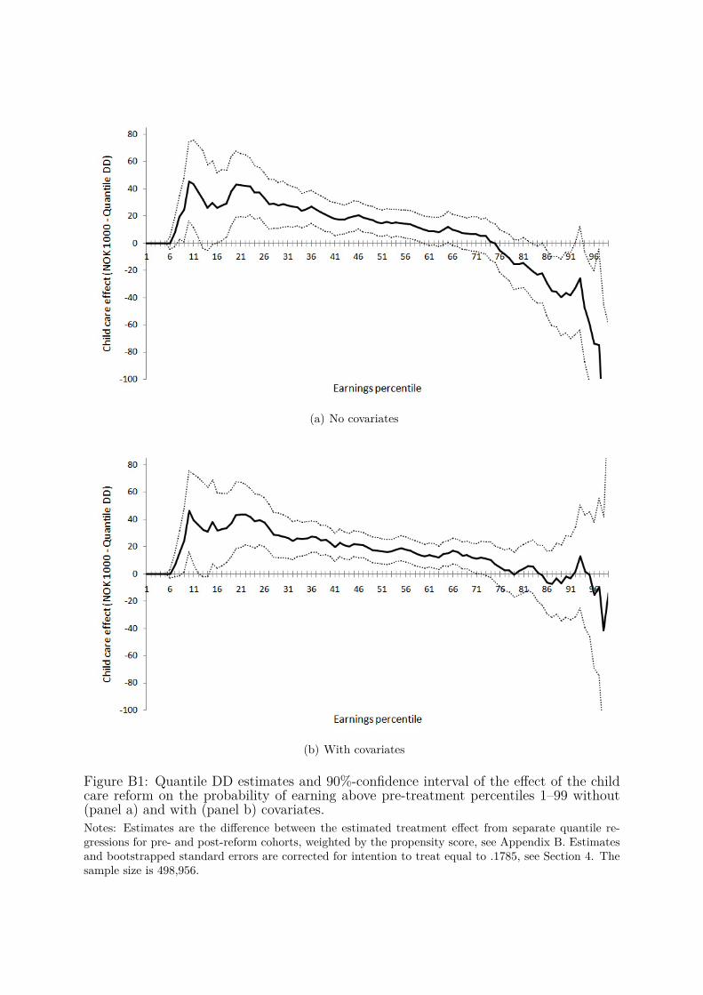
(a) No covariates

(b) With covariates

Figure B1: Quantile DD estimates and 90%-confidence interval of the effect of the childcare reform on the probability of earning above pre-treatment percentiles 1–99 without(panel a) and with (panel b) covariates.Notes: Estimates are the difference between the estimated treatment effect from separate quantile re-gressions for pre- and post-reform cohorts, weighted by the propensity score, see Appendix B. Estimatesand bootstrapped standard errors are corrected for intention to treat equal to .1785, see Section 4. Thesample size is 498,956.