Is it statistically

significant? Chi-square test

Dr Sam Cheadle and Dr Gosia Turner Student Data Management and

Analysis team

Tuesday 27 September 2016

This session:

• Theory behind chi-square test (20 minutes)

• Statistical and practical significance (5 minutes)

• Using the excel template to perform calculations (35

minutes)

• Questions (15 minutes)

Categorical variables• A basic unit that cannot be subdivided

indefinitely into equal units (gender, ethnicity, school type, division)

– Nominal

• Cannot be ranked (gender, ethnicity)

– Ordinal

• Can be ranked in some way (1st, 2.1, 2.2, 3)

The majority of data analysed by administrators at Oxford are categorical

Chi-square test

• The most appropriate statistical test to check if two categorical variables are independent.

– Gender difference in proportion of Firsts

– Differences in proportion of Firsts between divisions

– Differences in proportion of Firsts between Oxford Law and Cambridge Law

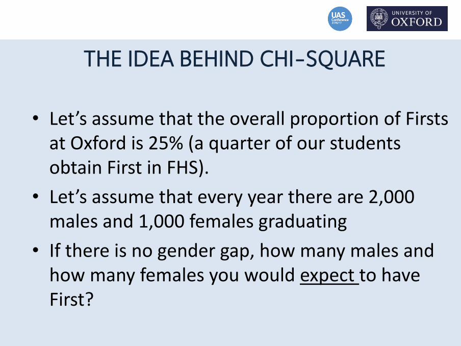
THE IDEA BEHIND CHI-SQUARE

• Let’s assume that the overall proportion of Firsts at Oxford is 25% (a quarter of our students obtain First in FHS).

• Let’s assume that every year there are 2,000 males and 1,000 females graduating

• If there is no gender gap, how many males and how many females you would expect to have First?

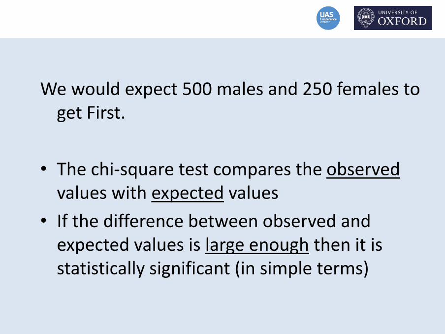
We would expect 500 males and 250 females to get First.

• The chi-square test compares the observed values with expected values

• If the difference between observed and expected values is large enough then it is statistically significant (in simple terms)

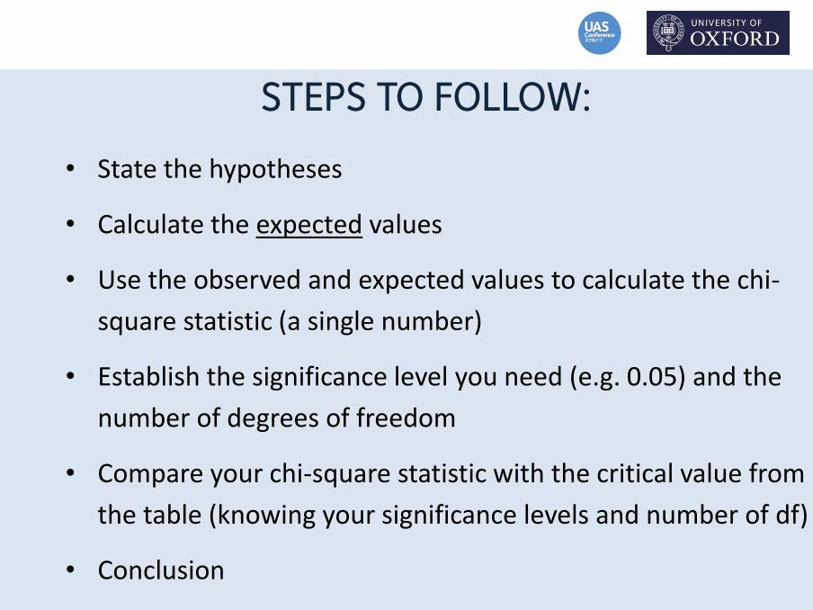
STEPS TO FOLLOW:

• State the hypotheses

• Calculate the expected values

• Use the observed and expected values to calculate the chi-

square statistic (a single number)

• Establish the significance level you need (e.g. 0.05) and the

number of degrees of freedom

• Compare your chi-square statistic with the critical value from

the table (knowing your significance levels and number of df)

• Conclusion

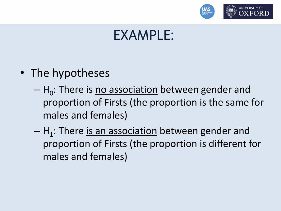
EXAMPLE:

• The hypotheses

– H0: There is no association between gender and proportion of Firsts (the proportion is the same for males and females)

– H1: There is an association between gender and proportion of Firsts (the proportion is different for males and females)

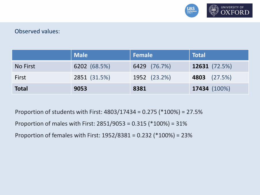
Observed values:

Male Female Total

No First 6202 (68.5%) 6429 (76.7%) 12631 (72.5%)

First 2851 (31.5%) 1952 (23.2%) 4803 (27.5%)

Total 9053 8381 17434 (100%)

Proportion of students with First: 4803/17434 = 0.275 (*100%) = 27.5%

Proportion of males with First: 2851/9053 = 0.315 (*100%) = 31%

Proportion of females with First: 1952/8381 = 0.232 (*100%) = 23%

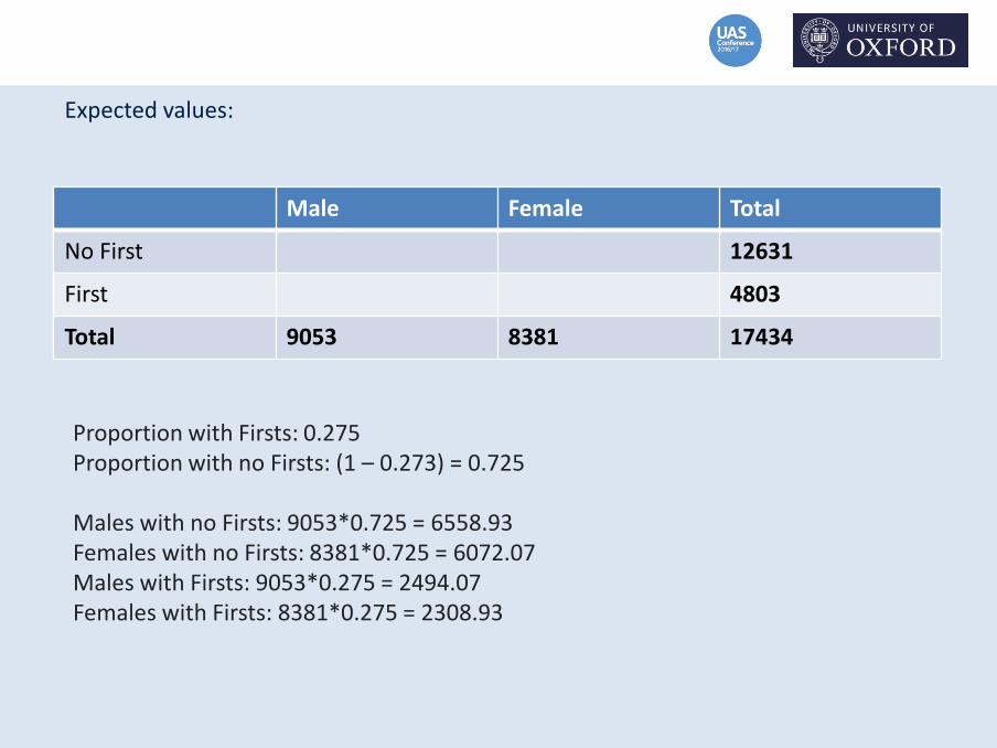
Expected values:

Male Female Total

No First 12631

First 4803

Total 9053 8381 17434

Proportion with Firsts: 0.275Proportion with no Firsts: (1 – 0.273) = 0.725

Males with no Firsts: 9053*0.725 = 6558.93Females with no Firsts: 8381*0.725 = 6072.07Males with Firsts: 9053*0.275 = 2494.07Females with Firsts: 8381*0.275 = 2308.93

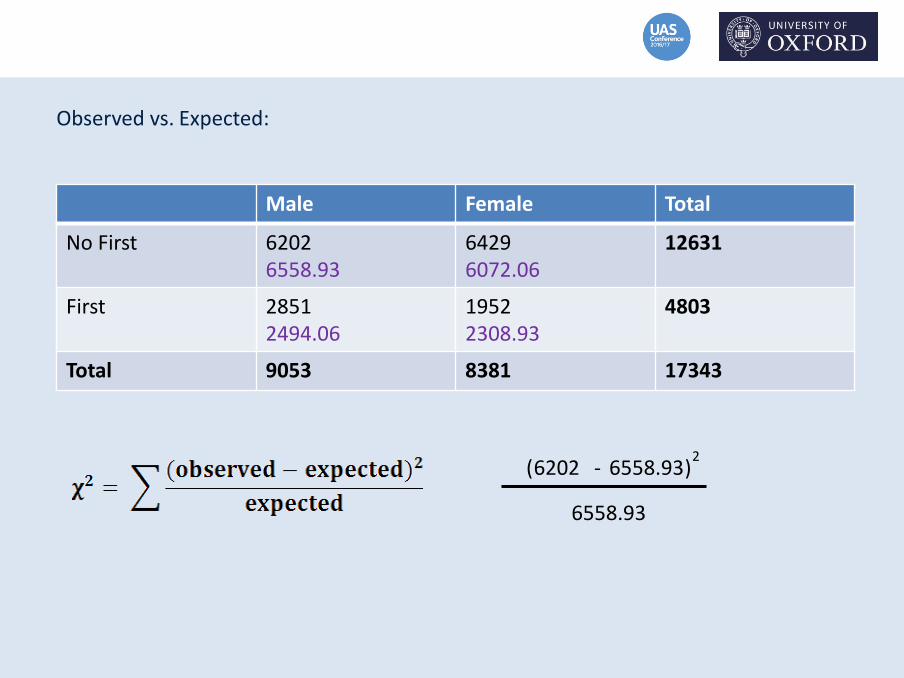
Observed vs. Expected:

Male Female Total

No First 62026558.93

64296072.06

12631

First 28512494.06

19522308.93

4803

Total 9053 8381 17343

6202 -( )

6558.93

26558.93

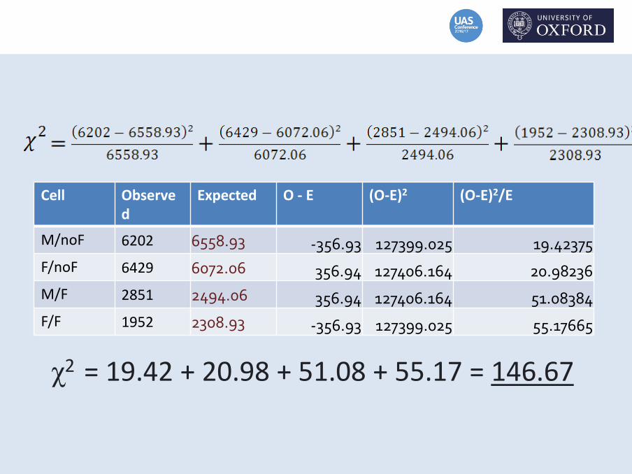
Cell Observed

Expected O - E (O-E)2 (O-E)2/E

M/noF 6202 6558.93 -356.93 127399.025 19.42375

F/noF 6429 6072.06 356.94 127406.164 20.98236

M/F 2851 2494.06 356.94 127406.164 51.08384

F/F 1952 2308.93 -356.93 127399.025 55.17665

χ2 = 19.42 + 20.98 + 51.08 + 55.17 = 146.67

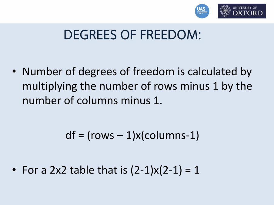
DEGREES OF FREEDOM:

• Number of degrees of freedom is calculated by multiplying the number of rows minus 1 by the number of columns minus 1.

df = (rows – 1)x(columns-1)

• For a 2x2 table that is (2-1)x(2-1) = 1

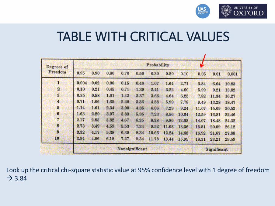
TABLE WITH CRITICAL VALUES

Look up the critical chi-square statistic value at 95% confidence level with 1 degree of freedom 3.84

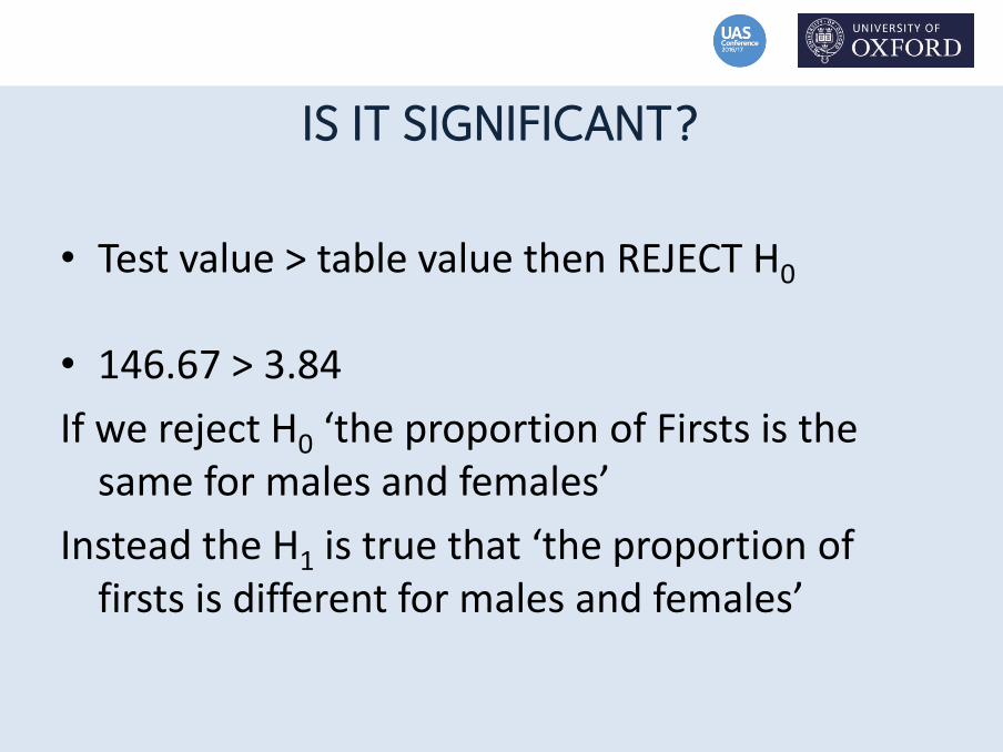
IS IT SIGNIFICANT?

• Test value > table value then REJECT H0

• 146.67 > 3.84

If we reject H0 ‘the proportion of Firsts is the same for males and females’

Instead the H1 is true that ‘the proportion of firsts is different for males and females’

RECAP

• Hypothesis

• Calculate table of expected values

• Calculate the test statistic

• Establish the number of df

• Find the critical value in the table (considering the significance level and the number of df)

• Compare your test value with the table value and make a decision

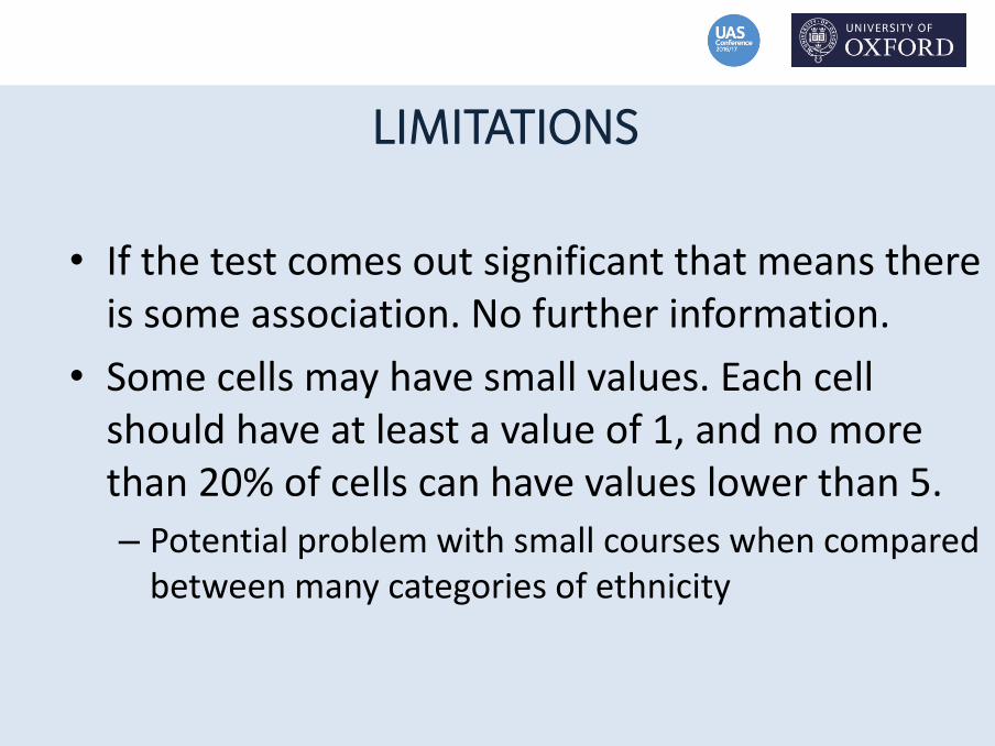
LIMITATIONS

• If the test comes out significant that means there is some association. No further information.

• Some cells may have small values. Each cell should have at least a value of 1, and no more than 20% of cells can have values lower than 5.

– Potential problem with small courses when compared between many categories of ethnicity

PRACTICAL VS STATISTICAL SIGNIFICANCE

Is it statistically

significant?

PRACTICAL VS STATISTICAL SIGNIFICANCE

Is it statistically

significant?Is it important?

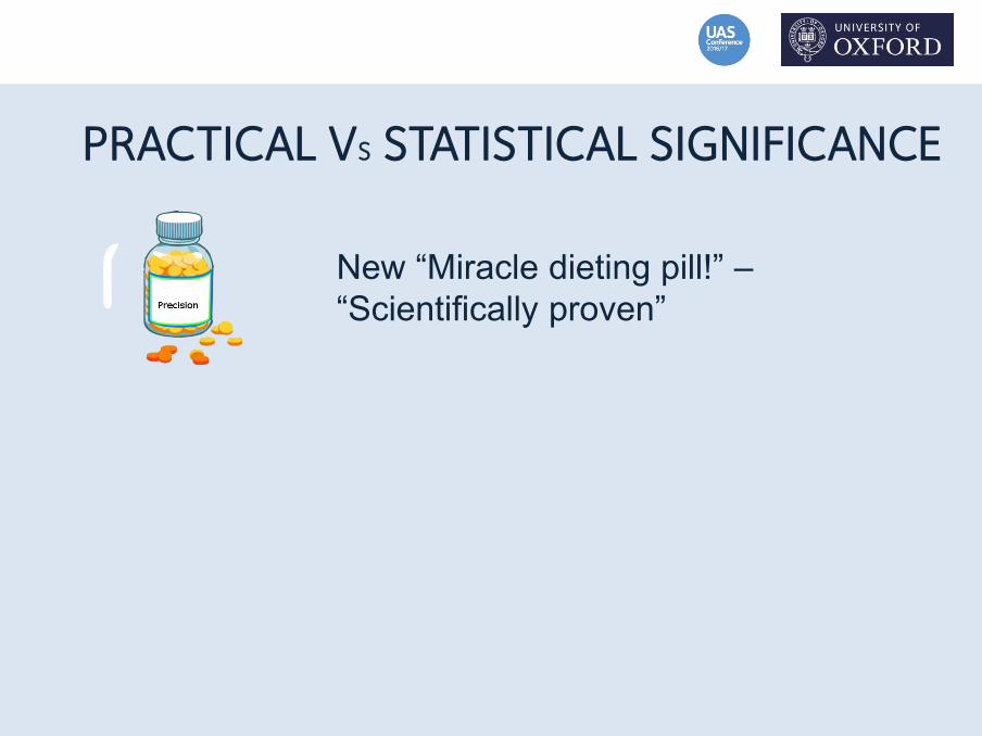
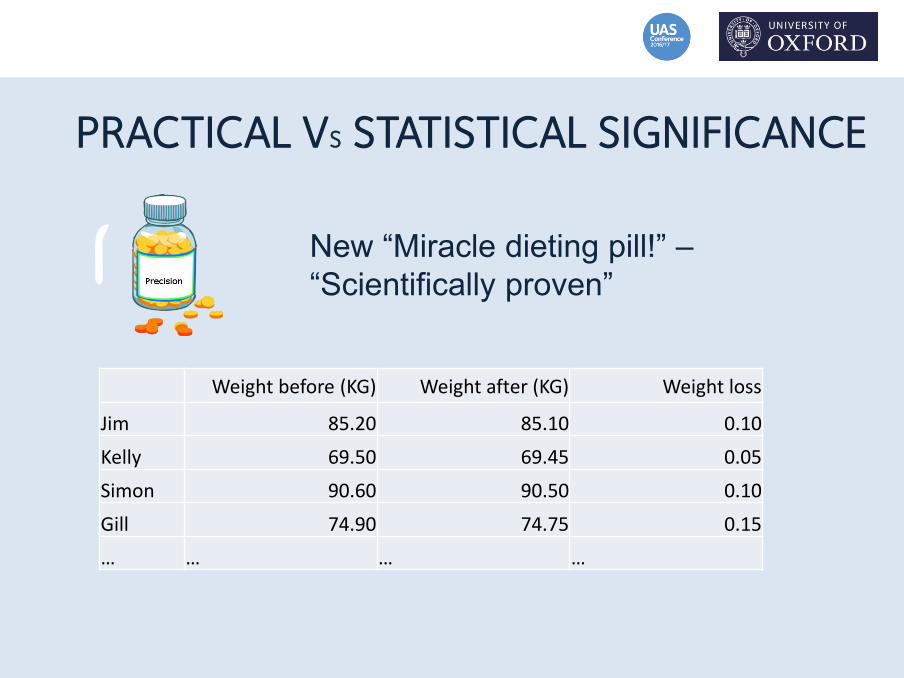
PRACTICAL VS STATISTICAL SIGNIFICANCE

New “Miracle dieting pill!” –

“Scientifically proven”

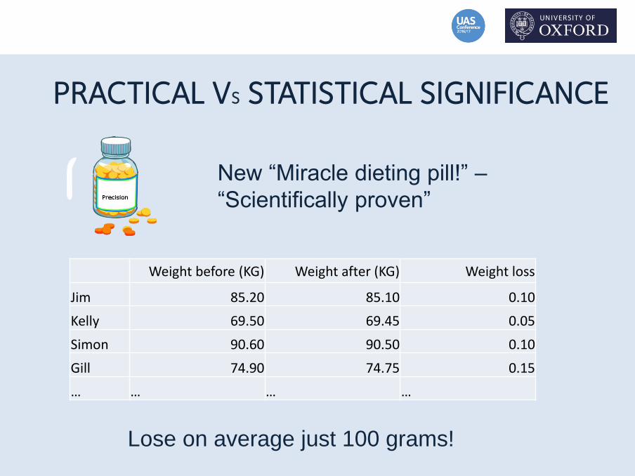
PRACTICAL VS STATISTICAL SIGNIFICANCE

New “Miracle dieting pill!” –

“Scientifically proven”

Weight before (KG) Weight after (KG) Weight loss

Jim 85.20 85.10 0.10

Kelly 69.50 69.45 0.05

Simon 90.60 90.50 0.10

Gill 74.90 74.75 0.15

… … … …

PRACTICAL VS STATISTICAL SIGNIFICANCE

New “Miracle dieting pill!” –

“Scientifically proven”

Weight before (KG) Weight after (KG) Weight loss

Jim 85.20 85.10 0.10

Kelly 69.50 69.45 0.05

Simon 90.60 90.50 0.10

Gill 74.90 74.75 0.15

… … … …

Lose on average just 100 grams!

PRACTICAL VS STATISTICAL SIGNIFICANCE

• Statistically significant effects are not

necessarily large.

PRACTICAL VS STATISTICAL SIGNIFICANCE

• Statistically significant effects are not

necessarily large.

• Statistical without practical significance.

PRACTICAL VS STATISTICAL SIGNIFICANCE

• Statistically significant effects are not

necessarily large.

• Statistical without practical significance.

• Practical without statistical significance (be

careful!).

QUESTIONS?