Is It Possible to Beat the Random Walk - redalyc.org · de previsões na tentativa de melhorar a...

Revista Brasileira de Finanças

ISSN: 1679-0731

[email protected]

Sociedade Brasileira de Finanças

Brasil

Fernandes Marçal, Emerson; Hadad Junio, Eli

Is It Possible to Beat the Random Walk Model in Exchange Rate Forecasting? More

Evidence for Brazilian Case

Revista Brasileira de Finanças, vol. 14, núm. 1, marzo, 2016, pp. 65-88

Sociedade Brasileira de Finanças

Rio de Janeiro, Brasil

Available in: http://www.redalyc.org/articulo.oa?id=305845303004

How to cite

Complete issue

More information about this article

Journal's homepage in redalyc.org

Scientific Information System

Network of Scientific Journals from Latin America, the Caribbean, Spain and Portugal

Non-profit academic project, developed under the open access initiative

http://www.redalyc.org/revista.oa?id=3058


http://www.redalyc.org/articulo.oa?id=305845303004

http://www.redalyc.org/comocitar.oa?id=305845303004

http://www.redalyc.org/fasciculo.oa?id=3058&numero=45303

http://www.redalyc.org/articulo.oa?id=305845303004


http://www.redalyc.org

Is It Possible to Beat the Random WalkModel in Exchange Rate Forecasting? MoreEvidence for Brazilian Case(É Possível Bater o Passeio Aleatório na Previsão da Taxa de Câmbio?Mais Evidência para o Caso Brasileiro)

Emerson Fernandes Marçal*Eli Hadad Junior**

Abstract The seminal study of Meese and Rogoff on exchange rate forecastabilityhad a great impact on the international finance literature. The authors showed thatexchange rate forecasts based on structural models are worse than a naive randomwalk. This result is known as the Meese–Rogoff (MR) puzzle. Although the vali-dity of this result has been checked for many currencies, studies for the Braziliancurrency are not common. In 1999, Brazil adopted the dirty floating exchange rateregime. Our goal is to run a “pseudo real-time experiment” to investigate whetherforecasts based on econometric models that use the fundamentals suggested by theexchange rate monetary theory of the 80s can beat the random model for the case ofthe Brazilian currency. Our work has three main differences with respect to Rossi(2013). We use a bias correction technique and forecast combination in an attemptto improve the forecast accuracy of our projections. We also combine the randomwalk projections with the projections of the structural models to investigate if it ispossible to further improve the accuracy of the random walk forecasts. However,our results are quite in line with her results. We show that it is not difficult to beatthe forecasts generated by the random walk with drift using Brazilian data, but thatit is quite difficult to beat the random walk without drift. Our results suggest that itis advisable to use the random walk without drift, not only the random walk withdrift, as a benchmark in exercises that claim the MR result is not valid.Keywords: Meese-Rogoff puzzle, forecasting, exchange rate.JEL Codes: F31, F32, F41, C51.

Submetido em 21 de fevereiro de 2016. Aceito em 24 de fevereiro de 2016. Publi-cado on-line em 21 de Abril de 2016. O artigo foi avaliado segundo o processo de duploanonimato além de ser avaliado pelo editor. Editor responsável: Márcio Laurini.

*Head of Center for Applied Macroeconomic Research at Sao Paulo School of Eco-nomics and CSSA-Mackenzie. E-mail: [email protected]

**Mackenzie Presbyterian University E-mail: [email protected]

Rev. Bras. Finanças (Online), Rio de Janeiro, 14, No. 1, March 2016, pp. 65-88ISSN 1679-0731, ISSN online 1984-5146

c©2016 Sociedade Brasileira de Finanças, under a Creative Commons Attribution 3.0 license -http://creativecommons.org/licenses/by/3.0

Marçal, E. F., Junior, E. H.

Resumo

O trabalho seminal de Meese e Rogoff sobre previsibilidade da taxa de câmbio tevegrande impacto na literatura de finanças internacionais. Os autores mostraram queprevisões baseadas em modelos econômicos estruturais tinham um desempenhopior que um passeio aleatório ingênuo. Este resultado é conhecido na literaturacomo o quebra-cabeça de Meese-Rogoff. Ainda que a validade deste resultadotenha sido checado para um número grande de moedas, estudos para a moeda bra-sileira ainda não são tão comuns pois o Brasil adotou o regime de câmbio flexívelapenas a partir de 1999. Rossi (2013) realizou um estudo amplo do quebra-cabeçaproposto pelos autores mas não fez a análise dos dados brasileiros. O objetivodeste trabalho é simular um exercício de tempo real para investigar se as previsõesbasedas em modelos econômicos de determinação de taxa de câmbio que usam osfundamentos dos modelos desenvolvidos nos anos oitenta tem desempenho melhorque o modelo de passeio aleatório. O trabalho tem três diferenças principais emrelação ao feito por ela. Utiliza-se a técnica de correção de viés e de combinaçãode previsões na tentativa de melhorar a precisão das previsões. Também combina-se as previsões do passeio aleatório com as dos modelos estruturais. Entretanto osresultados obtidos continuam em linha com da autora. O presente trabalho mostraque não é difícil gerar previsões com melhor desempenho que um passeio aleatóriocom tendência (drift) mas é extremamente difícil bater o desempenho do passeioaleatório ingênuo (sem tendência). O trabalho sugere que é fortemente recomen-dado utilizar o passeio aleatório sem tendência em exercícios que visem avaliar oquebra-cabeça de Meese e Rogoff.Palavras-chave: Meese-Rogoff puzzle, previsão, taxa de câmbio.

1. Introduction

The seminal study of Meese & Rogoff (1983) on exchange rate fore-castability had a great impact on international finance literature. The au-thors compared exchange rate projections obtained from structural modelsagainst a naive random walk. They used structural monetary models of the80s.1 Their main result showed that it is not easy to outperform forecasts ofa naive random walk model. Subsequently, an extensive literature emerged,but the result of Meese & Rogoff (1983) still holds. This is the so-calledMeese–Rogoff (MR) puzzle.

In a recent paper, Rossi (2013) reviewed the literature that followedthe work of Meese and Rogoff, aiming to confirm and explain their result.Rossi (2013) showed that it is still difficult to beat the random walk, partic-ularly in an out-of-sample exercise. She ran a comprehensive exercise with

1See, for example, Frenkel (1976), Dornbusch (1976), Frankel (1979), and Hooper &Morton (1982).

66 Rev. Bras. Finanças (Online), Rio de Janeiro, V14, No. 1, March 2016

Is It Possible to Beat the Random Walk Model in Exchange Rate Forecasting? More Evidencefor Brazilian Case

different sets of fundamentals, econometric model specifications, samples,and countries. She showed that the MR puzzle still holds, particularly in anout-of-sample exercise. However, she did not include Brazil in her research.

The purpose of our paper is to run an exercise similar to Rossi (2013)using Brazilian data. We focus our analysis on multivariate econometricmodels with monetary fundamentals. In addition, we opt to run a forecastexercise using bias correction and forecasting combination techniques. Wecombine the forecasts of the models among themselves and with the ran-dom walk. We perform a pseudo real-time exercise to replicate, as closelyas possible, the forecast that one could have carried out at a particular timein the past. We use the Model Confidence Set (MCS) algorithm developedby Hansen et al. (2011) to evaluate the predictive equivalence of the fore-casts.

Our results suggest that the MR puzzle holds for Brazilian data. It ishard to beat the random walk without drift for almost all analysed horizonsfrom one up to six quarters. Moreover, it is much easier to beat the randomwalk with drift than without drift.

The paper is divided into six sections. The first section is this introduc-tion. The second section discusses the strategy for constructing forecastsusing the fundamentals suggested by the model of the 80s. In the thirdsection, the MCS algorithm is described. In the fourth section, we brieflydiscuss the results of Rossi (2013) and some key references regarding theMR puzzle. The fifth section presents the results of our empirical exerciseand compares them with the literature. Finally, some concluding remarksare drawn.

2. Constructing a strategy to forecast exchange rate

In this section, we briefly describe the equation used to construct fore-casts based on the monetary exchange rate models of the 80s as well as oneconometric models.

2.1 The random walk model

In this study, the goal is to compare forecasts obtained from the randomwalk models with and without drift against a wide array of econometricmodels. The random walk model with drift is given by

yt = yt−1 + a+ εt (1)

Rev. Bras. Finanças (Online), Rio de Janeiro, V14, No. 1, March 2016 67


where εt is a random variable with zero mean that is independent overtime. The model without drift can be obtained by assuming that a=0.

The k steps ahead forecast is given by

Et[yt+k] = yt + a ∗ k (2)

2.2 The structural models of the 80s

In addition to the aforementioned random walk models, this study usesvector autoregressive models with and without an error correction mech-anism in order to construct forecasts.2 The choice of which explanatoryvariables to include in the models is made based on the economic modelsof the 80s and 90s that served as a basis for the article of Meese and Rogoff.Some key references are Frenkel (1976), Bilson (1978), Dornbusch (1976),and Frankel (1979).

These models link the exchange rate to a set of fundamentals. Themodel of the 80s implies an equation similar to (3), with different restric-tions imposed on the coefficients according to variants of the basic model:

et=β0+β1(yt−y∗t )+β2(it−i∗t )+β3(mt−m∗t )+β4(πt−π∗

t )+β5(pt−p∗t )+vt (3)

where et denotes an exchange rate between countries i and j, yt−y∗t thedifference in the real income,mt−m∗t the difference in monetary aggregate,and πt − π∗t the difference in inflation rates. vt is a random variable withzero mean.

2.3 Single-equation models

The first step in constructing a forecast based on (3) is to estimate theparameters using some econometric technique. Ordinary least square is onecommon choice in the literature, but others techniques can be used as well.

We calculate the expectations based on the information available at timet-1.

Et−1(et)=β0+Et−1[β1(yt−y∗t )+β2(it−i∗t )+β3(mt−m∗t )+β4(πt−π∗

t )+β5(pt−p∗t )] (4)

Assuming that it is not possible to predict any change in the fundamen-tal using the information available until t-1, the forecast for the exchangerate in t based on information t-1 is given by (5):

2One can see Enders (2008) for a textbook explanation.



Et−1(et) = β0 + β1(yt−1 − y∗t−1) + β2(it−1 − i∗t−1) + β3(mt−1 −m∗t−1)+

β4(πt−1 − π∗t−1) + β5(pt−1 − p∗t−1)]

(5)

The forecasts are constructed using (5). It is also possible to predicta change in fundamentals using past information. If this is the case, aneconometric model can be formulated, which leads us to the multivariateequation approach.

2.4 Multiple-equations models

Two different econometrics models are used in this paper. The first isthe vector autoregressive (VAR) model, and the second is the vector errorcorrection (VEC) model.

2.4.1 VAR model

One possible way of modelling the exchange rate and the fundamentalis to use a VAR model:

Yt = Π1Yt−1 + ...+Πk−1Yt−k+1 + τ + εt (6)

where εt are random normal and uncorrelated errors, Ω denotes the varianceand covariance matrix of the errors that do not vary with time, and θ =[Π1, ...,Πk, τ ] contains the parameters of the model. The vector Yt containsthe exchange rate and set of fundamentals chosen by the analyst.

2.4.2 VEC model

We assume that the local data generation process for the exchange rateand a set of fundamentals is given by the following VAR model:

∆Yt = Γ1∆Yt−1 + ...+ Γk−1∆Yt−k+1 + αβ′Y t−1 + µ+ εt (7)

where εt are random normal and uncorrelated errors, Ω denotes the varianceand covariance matrix of the errors that do not vary with time, and θ =[Γ1, ...Γk−1, α, β, µ] contains the parameters of the model. The vector Ytcontains the exchange rate and set of fundamentals chosen by the analyst.∆denotes the first difference.



2.5 Bias correction approach

One way to improve the forecast performance of a particular model isthe bias correction approach. If one model systematically forecasts in onewrong direction, the analyst can, ideally, correct the forecast by adding aterm to avoid the bias.

Our approach is inspired by the paper of Issler & Lima (2009). Supposethat we want to forecast the exchange for t+1 with information availableuntil t. We compute forecasts for a window of length τ from t− τ to t andcollect all errors of these forecasts. Using an average of these errors (bc)and under certain conditions, this simple average will provide a consistentestimate of the bias.

Our bias-corrected forecast is calculated by the following formula:

tFBCt+h =t F t+h − bc (8)

where h>0 denotes the horizon of the forecast.

2.6 Combined forecast techniques

Granger & Ramanathan (1984) and Bates & Granger (1969) suggestedthat a combination of two forecasts can generate more precise forecasts.There is extensive literature discussing alternative methods for combiningforecasts. In this paper, we opt to use a simple combination technique. Wecombine each pair of forecasts using a simple average. We aim to evaluatewhether this simple technique pays off. In her empirical exercise, Rossi(2013) did not use any forecast combination; nor did the seminal paper ofMeese & Rogoff (1983).

We explore two types of combinations. The first is a combination ofall possible pairs of structural model forecasts. The second combines therandom walk forecast with each structural model forecast. If any structuralmodel contains relevant information regarding the future, it may not beable to beat the random walk; however, combined with it, the projectionmay outperform the random walk. We aim to investigate if it is possible tofurther improve the predictive power of the random walk.

3. How to choose among different forecast models

In this section, we discuss two criteria used to compare the predictiveforecasts of different models. The first is the classical Diebold-Marianotest Diebold & Mariano (1995). The second is the model confidence set



developed by Hansen et al. (2011). The latter can be seen as a refinementof the former test.

3.1 Classical Diebold–Mariano test

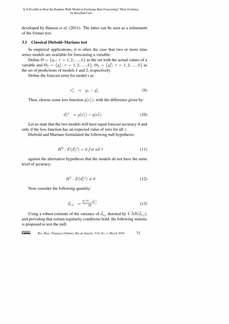
In empirical applications, it is often the case that two or more timeseries models are available for forecasting a variable:

Define Θ = yτ ; τ = 1, 2, ...., k as the set with the actual values of avariable and Θ1 = y1

τ ; τ = 1, 2, ...., k, Θ2 = y2τ ; τ = 1, 2, ...., k as

the set of predictions of models 1 and 2, respectively.Define the forecast error for model i as:

eiτ = yτ − yiτ (9)

Then, choose some loss function g(eiτ ), with the difference given by:

di,jτ = g(eiτ )− g(ejτ ) (10)

Let us state that the two models will have equal forecast accuracy if andonly if the loss function has an expected value of zero for all τ .

Diebold and Mariano formulated the following null hypothesis:

H0 : E(di,jτ ) = 0 for all τ (11)

against the alternative hypothesis that the models do not have the samelevel of accuracy:

H1 : E(di,jτ ) 6= 0 (12)

Now consider the following quantity:

di,j =∑Mτ=1 d

i,jτ

M (13)

Using a robust estimate of the variance of di,j denoted by ˆV AR(di,j),and providing that certain regularity conditions hold, the following statisticis proposed to test the null:



DM =di,j√ˆV AR(di,j)

a∼ N(0, 1) (14)

One serious limitation of the Diebold-Mariano framework is that it isnot designed to deal with many different competing models simultaneously.If there is a benchmark, all remaining models could be compared againstthe benchmark. However, if the analyst wants to rank the models and hasno particular interest in choosing a benchmark, another framework shouldbe tried. Hansen et al. (2011) tries to fill this gap.

3.2 The model confidence set

The model confidence set (MCS) is a model selection technique de-veloped by Hansen, Lunde, and Nason (2011). It consists of an algorithmthat ranks the forecasts from models. M∗ contains the best model(s) cho-sen from a collection of models, M0, in which the “best model” is definedusing criteria related to prediction quality.

Definition 1: The set of superior objects is defined by:M∗ ≡ i εM0 : E(di,jτ ) ≤ 0 for all j εM0In the following, we let M † denote the complement to M∗. That is,

M † ≡ i εM0 : E(di,jτ ) > 0 for all j εM0The MCS selects a model using an equivalence test, δM , and an elimi-

nation rule, %M . The equivalence test is applied to the set M = M0. If theequivalence hypothesis is rejected, then there is evidence that there is a setof inferior models in terms of forecast accuracy. Therefore, the rule %M isused to eliminate the models with poor predictive quality. The procedure isrepeated until the equivalence test, δM , is accepted. Then, the model (M∗F )is selected to be the set of the best final models.

The null hypothesis of the test is:

H0M : E(di,jτ ) = 0 for all i, j ε M (15)

where M ⊂M0.The alternative hypothesis is:

H1M : E(di,jτ ) 6= 0 for some i, j ε M (16)

Note that there might be better models outside of the set of “candidatemodels”, M0. The goal of the MCS is to determine M∗.



The null hypothesis can be tested using the following statistic:3

TD =∑i εM

t2i (17)

where ti = di√ˆV AR(di)

and di ≡M−1∑

j εM dij

The statistic given by (17) has a non-standard distribution that can besimulated using bootstrap techniques.

The elimination rule is:

%M = argmaxi(ti) (18)

3.2.1 The algorithm

The MCS algorithm takes the following steps:(i) Initially set M = M0;(ii) Test H0

M using δM at level α;(iii) If H0

M is not rejected then the procedure ends and the final set isM∗1−α = M , otherwise we use %M to eliminate an object from M andrepeat step (i).

The authors show that the MCS has the following statistical properties:(i) limn→∞P (M∗ ⊂ M∗1−α) > 1− α and(ii) limn→∞P (i† ε ⊂ M∗1−α) = 0 for all i† ε ⊂M †

3.2.2 Ranking the models: MCS p-values

The elimination rule, %M , defines a sequence of random sets, M0 =M1 ⊃M2 ⊃ ... ⊃Mm0, whereMi = %i, ..., %m0 andm0 are the numberof elements inM0. %M0 is the first to be eliminated, %M1 is the second to beeliminated, and so forth. At the end, only one model survives. We set thep-value of this model as 1. We collect the p-value of the eliminated modelif it is higher than the p-value of the previously eliminated model. If it isnot, we opt to maintain the p-values of the previous rejections.

The MCS p-values are convenient because they make it easier for theanalyst to determine whether a particular object is in M∗1−α.

3There are others possible choices.



3.3 Pseudo real-time exercise

The data gathered for the countries is used to create many variants ofthe structural models in order to forecast the exchange rate. The sampleis split into two parts. The first half of the sample is used to estimate themodels, and the second half is used to evaluate the forecast performance ofthe models in various horizons. In the exercise, we attempt to simulate areal-time operation. We use an information set that reflects, as closely aspossible, the one available to agents at the time of the forecast. In otherwords, the models are re-estimated at each point in order to incorporate thenew information arriving at each instant of time. For each model, forecastsare generated for up to six quarters (a year and a half). All of the projectionsperformed by the models are grouped according to time horizon. Thus,there are six groups — one for each horizon.

Some of the data we collected are revised from the initial publicationin their original sources. The values we use to run our projections are notexactly the same as those available to agents at that time. We run projec-tions in our pseudo real-time experiment with a slightly better informationset. This may result in better forecast accuracy compared to the projectionsgenerated in real time. Because a dataset with original published data is notavailable, this is the best we can do to simulate a real exercise.

4. Meese–Rogoff Puzzle

A comprehensive survey on the literature that followed the study ofMeese & Rogoff (1983) was conducted by Rossi (2013). Her main conclu-sions are as follows:

1. There is a consensus in the literature that models based on the Taylorrule and that use the net foreign assets position produce better fore-casts outside the sample than do other traditional fundamentals, suchas interest rates, inflation, gross domestic product, and differentialsbetween monetary aggregates. The monetary fundamentals in longhorizons and the interest rate differentials in short horizons have pre-dictive power in some studies, but not in others. However, there aredifferences of opinion regarding whether monetary fundamentals areuseful, as suggested by Meese and Rogoff.

2. Among all the classes of model, those with the best performanceare linear and error-correction models. For single-equations models,



explanatory variables are more relevant than lagged, contemporary,or historical data are.

3. Data transformations, such as seasonal adjustments, lags, de-trending,and differentiations can substantially affect the predictive power ofthe model, and can explain why there are differences in results be-tween studies. For example, consider the forecasting ability of themonetary model in long horizons. For some fundamentals, the fore-casting ability changes significantly when historical data is replacedwith real-time data. For some models, the forecasting ability alsoappears to depend on the chosen country. With few exceptions, thefrequency of data and whether they are historical or projected appearnot to affect the forecasting ability of the model.

4. The choices of benchmark, projection time horizon, data sample, andprojection method are very important. The random walk without driftis the most difficult benchmark to beat.

5. On one hand, the empirical analysis confirms most of the foreignexchange studies. Due to instability in the parameters of the modelsused, some variables have forecasting ability within the sample butdo not have projection relevance outside of the sample. Moreover,the predictive power of models varies between countries, models andvariables used, period of time analysed, and data sample. Althoughthe Taylor rule and the net foreign assets variable have forecastingability for short periods of time, and other models based on monetaryfundamentals (error-correction models) have forecasting ability forlonger time horizons, none of them appears to discard the conclusionsof Meese and Rogoff.

Another important point to be addressed comes from the papers of En-gel & West (2005) and Engel et al. (2007). They showed that under reason-able parameters configuration, the exchange rate models reflect dynamicsthat are similar to those a near random walk. If they were correct, oneimplication of the monetary exchange rate approach is poor out-of-samplepredictive performance. They suggested that the MR puzzle should not beseen as evidence against these models.



5. Results

5.1 Database description

The study aims to analyse the forecast performance of a set of mod-els to predict the nominal exchange rates between the Real and a set ofcurrencies: Real–Dollar, Real–Yen, and Real–Pound pairs are analysed.The datasets for the analysis were collected from the DATASTREAM datasystem (Thomson-Reuters) and the International Monetary Fund’s (IMF’s)International Financial Statistics (IFS) database.

The frequency of the data is quarterly. The period covers the years from1995 to 2013. The fundamentals are gross domestic product (GDP), mon-etary aggregates (M1 and M2), consumer price index (CPI, and net foreignasset position as a share of GDP. The data of the net foreign asset posi-tion are gathered from Lane & Milesi-Ferretti (2001) and updated basedon the IFS database. All of the models are estimated using the STATA-12program. The analysis of the results and the choice of the best models areperformed via the MCS Hansen et al. (2011) and implemented in the Ox-metrics 6 program through the code made available by the authors via theirwebpage.

5.2 Results and Discussion

5.2.1 The U.S. Dollar–Brazilian Real case

We estimated a VAR model and a VEC model with and without sea-sonal dummies for 18 different combinations of the fundamentals. Thisresulted in a total of 72 models. We then performed the bias correction pro-cedure for all of these models, bringing the total to 144 models. Next, wecombined all of the models in pairs. We also combined the random walkforecast with and without drift with each previous model. This yielded atotal of 10,730 model forecasts. The forecasts were ranked by their meanforecast squared error (MFSE). The random walk with and without driftwere also included. We collected the forecasts for all horizons from one tosix quarters ahead. All of these models were re-estimated at each point intime in our pseudo real-time data experiment.

Because we had too many forecasts to compare, we opted to run a pre-liminary selection round using the MFSE. The forecasts were ranked bytheir MFSE in ascending order. The first 250 best models were selectedand classified for the second round. In the second round, we ran the MCSalgorithm to define the best forecasts. If the random models with or with-



out drift were not classified in the first round, we opted to award them awildcard. They were always included in the MCS round.

Multivariate models versus random walk The results of this pseudoreal-time experiment can be seen in Table 1. The MCS algorithm classi-fied the random walk without drift as the best forecast for all horizons. Forshorter horizons, there were other forecasts that could be seen as at leastas good as the random walk, but with higher MFSE. As for the forecastsfrom one to three quarters, some models were considered equivalent to therandom walk. However, for horizons from four to six quarters, the randomwalk was the best model to forecast the exchange rate. All other modelswere eliminated from the final set. The set of fundamentals that seemedto generate some forecastability contained monetary aggregates, gross do-mestic product, and net foreign asset position. Finally, the random walkwith drift was eliminated from all final sets. This last result is in line withRossi (2013). She claimed that the random walk without drift is the hardestbenchmark to beat.

Full set of forecasts versus random walk The results of the completedpseudo real-time experiment can be seen in Table 2. The MCS algorithmclassifies the random walk without drift as the best forecast for all horizons.Contrary to the previous case, there are other forecasts that can be seen as atleast as good as the random walk, but with higher MFSE, up to five quarters.For the six-quarters-ahead forecast, the random walk is the only model inthe MCS final set. The random walk with drift was eliminated from allfinal sets. This last result is line with Rossi (2013). The bias correctionprocedure did not seem to add relevant forecastability to the models. Noneof them were selected in all horizons. Some combined forecast models arein the final set. The finalists include pairs of multivariate models as well aspairs that combine a multivariate model with a random walk without drift.Nonetheless, even in this broader experiment, it is not possible to beat therandom walk if the mean squared error is the metric.

5.3 Robustness check

Almost all transactions that involved the Brazilian currency were per-formed against the Dollar. However, we ran a similar exercise, looking tothe bilateral exchange rate of the Real against the British Pound and theJapanese Yen.



Tabl

e1

MC

Sre

sults

fort

heca

seof

mul

tivar

iate

mod

els

vers

usra

ndom

wal

k—

Bra

zila

ndth

eU

nite

dSt

ates

.



Tabl

e2

MC

Sre

sults

fort

heca

seof

the

full

seto

ffor

ecas

tsve

rsus

rand

omw

alk

—B

razi

land

the

Uni

ted

Stat

es.



5.3.1 The Japanese Yen–Brazilian Real case

Multivariate models versus random walk Table 3 shows the results ofthe pseudo real-time experiment regarding the exchange rate of Brazil andJapan. For all horizons, the random walk is not the best model when themetric is the MFSE. For one, two, and five quarters ahead, the random walkhas the lowest mean squared error. For the other periods, the random walkis not the best model. Looking at the MCS results, the random walk is partof the final set at all horizons. The models that beat the random walk interms of mean squared error contain the following fundamentals: monetaryaggregates, net foreign asset position, and interest rate differential. Thelist of fundamentals that generates models with predictive power includesmonetary aggregates and net foreign asset position.

Full set of forecasts versus random walk Table 4 shows the results ofthe exercise using all of the forecasts. Here, the random walk is no longerthe best model. For the horizons one, two, three, and five quarters ahead, thebest model using the MFSE criteria is a model that combines the randomwalk and some structural model. For the four quarters ahead forecast, thebest model is a combination of two structural models with bias correction.Finally, for six quarters ahead, the best model is a structural model. Thefinal set contains many models at all horizons, but random walk is amongthem. These results contrast with the Brazil–United States case analysedpreviously. However, we must stress that Japan and Brazil are not engagedin major trade and financial relationships with each other.

5.3.2 The British Pound–Brazilian Real case

Multivariate models versus random walk Table 5 shows the results forBrazil and the United Kingdom. The random walk model is the best modelwhen the criteria is the MFSE. At shorter horizons, from one up to threequarters ahead, the final set contains not only the random walk but someothers models as well. At the horizon from four to six quarters ahead, therandom walk is the only element in the final set. The fundamentals that mayhelp to forecast the exchange rate are monetary aggregates, net foreign assetposition, real GDP, and interest rate.

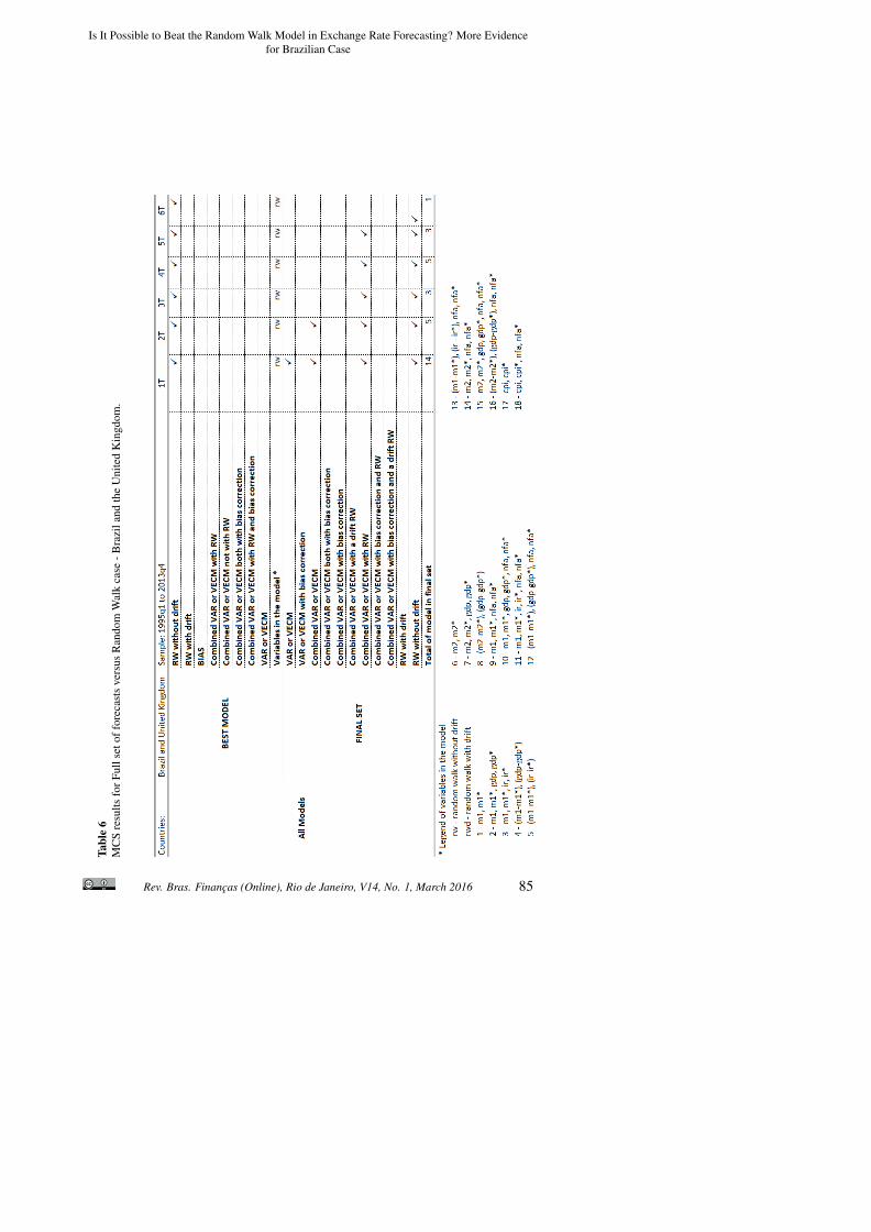
Full set of forecasts versus random walk Table 6 shows the results forBrazil and the United Kingdom using all of the models. The random walkmodel is the best model when the criteria is the MFSE for all horizons. The



Tabl

e3

MC

Sre

sults

fort

heca

seof

mul

tivar

iate

mod

els

vers

usra

ndom

wal

k—

Bra

zila

ndJa

pan.



Tabl

e4

MC

Sre

sults

fort

heca

seof

the

full

seto

ffor

ecas

tsve

rsus

rand

omw

alk

—B

razi

land

Japa

n.



final set includes combined models that have a random walk without driftin the pair. None of the models with bias correction appears in the final set.At six quarters ahead, the random walk is the lone element in the final set.In the horizons from one to five quarters ahead, the random walk is not theonly model in the final set.

5.4 Limitations, comparison with other studies, and paths for futureresearch

Some studies have investigated the MR puzzle using Brazilian data.Perdomo & Botelho (2007) tested the random walk hypothesis for the Brazil-ian case by comparing the error of exchange rate projections performed bybanks, consulting firms, and financial institutions. They used forecast datacollected by the Brazilian Central Bank (FOCUS) from the top-5 forecast-ers. Their study included projections of a random walk model for threeforecast horizons. The authors concluded that the random walk is moreaccurate than the models used by financial institutions.

Moura et al. (2008) reported the results of an out-of-sample exercise topredict the Brazilian exchange rate using the fundamentals and techniquesemployed for this paper. They also investigated Taylor rule models,4 in-spired by the papers of Engel, Mark, and West (2007), Mark (2007), Clar-ida and Waldman (2007), and Molodtsova and Papell (2007). They ran theDM test to compare the forecasts of the model with the benchmark of a ran-dom walk with drift. They reported that some models beat the benchmarkfor horizons up to 12 months. However, they did not report an exercise thatuses the random walk without drift as a benchmark. Based on our results,their benchmark may not be the hardest one to beat. It is possible that thattheir results may have been different if they opted to use the random walkwithout drift as a benchmark. In our exercise, we show that the randomwalk with drift is an easy benchmark to beat for Brazil.

Galimberti & Moura (2013) also reported results for Brazil. They anal-ysed a group of emerging market countries using a panel data technique.They showed evidence in favour of Taylor rule models and against the ran-dom walk with drift for Brazil and others countries. However, they too didnot report results for the toughest benchmark (i.e., the random walk withoutdrift).

Our paper focuses on models based on purchasing power parity, a mon-etary approach to the exchange rate. However, in future research, we can

4Taylor (1993)



Tabl

e5

MC

Sre

sults

fort

heca

seof

mul

tivar

iate

mod

els

vers

usra

ndom

wal

k—

Bra

zila

ndth

eU

nite

dK

ingd

om.



Tabl

e6

MC

Sre

sults

forF

ulls

etof

fore

cast

sve

rsus

Ran

dom

Wal

kca

se-B

razi

land

the

Uni

ted

Kin

gdom

.



investigate whether Taylor rule–based models can help to predict the ex-change rate in Brazil and whether they can outperform the random walkmodels both with and without drift.

One source of forecast failure in economics is a not-modelled change inthe mean of the data generation process (DGP). An automatic model selec-tion algorithm, such as Autometrics5 can be helpful in improving forecastaccuracy. Castle et al. (2014) discussed how to increase the robustness of aforecast obtained from a VEC model with a change in mean. This approachcan be tested to investigate whether forecasts from a VEC model with mon-etary exchange rate fundamentals can be improved using their procedure.

6. Final Remarks

The main goal of this paper was to investigate whether the models ofthe 80s can outperform the predictions from the random walk model forBrazil. The main conclusion of our paper is that the random walk modelwithout drift is the most difficult benchmark to be beat. In our exercise,we were able to outperform the random walk with drift, but not the randomwalk without drift.

Our results are in line with Rossi (2013), but our work differs from hersin the following aspects: (a) we used the MCS algorithm to investigate theforecast equivalence among the models; (b) we implemented a bias forecastcorrection in order to improve the forecasts; and (c) we also attempted asimple forecast combination technique. The random walk puzzle seems tohold for Brazilian data. The investigation of the predictive power of Taylorrule models is left for future research.

References

Bates, John M, & Granger, Clive WJ. 1969. The combination of forecasts.Or, 451–468.

Bilson, John FO. 1978. Rational expectations and the exchange rate. Theeconomics of exchange rates: Selected studies, 75–96.

Castle, Jennifer, Hendry, David, & Clements, Michael P. 2014 (Jan.). Ro-bust Approaches to Forecasting. Economics Series Working Papers 697.University of Oxford, Department of Economics.

5Hendry & Doornik (2013)



Diebold, Francis X, & Mariano, Robert S. 1995. Comparing PredictiveAccuracy. Journal of Business & Economic Statistics, 13(3), 253–263.

Dornbusch, Rudiger. 1976. Expectations and exchange rate dynamics. TheJournal of Political Economy, 1161–1176.

Enders, Walter. 2008. Applied econometric time series. John Wiley & Sons.

Engel, Charles, & West, Kenneth D. 2005. Exchange Rates and Fundamen-tals. Journal of Political Economy, 113(3), 485–517.

Engel, Charles, Mark, Nelson C., & West, Kenneth D. 2007 (Aug.). Ex-change Rate Models Are Not as Bad as You Think. NBER Working Pa-pers 13318. National Bureau of Economic Research, Inc.

Frankel, Jeffrey A. 1979. On the mark: A theory of floating exchange ratesbased on real interest differentials. The American Economic Review,610–622.

Frenkel, Jacob A. 1976. A monetary approach to the exchange rate: doc-trinal aspects and empirical evidence. the scandinavian Journal of eco-nomics, 200–224.

Galimberti, Jaqueson K., & Moura, Marcelo L. 2013. Taylor rules andexchange rate predictability in emerging economies. Journal of Interna-tional Money and Finance, 32(0), 1008 – 1031.

Granger, Clive WJ, & Ramanathan, Ramu. 1984. Improved methods ofcombining forecasts. Journal of Forecasting, 3(2), 197–204.

Hansen, Peter R, Lunde, Asger, & Nason, James M. 2011. The modelconfidence set. Econometrica, 79(2), 453–497.

Hendry, David F., & Doornik, Jurgen A. 2013. Empirical Model Discoveryand Theory Evaluation. MIT Press.

Hooper, Peter, & Morton, John. 1982. Fluctuations in the dollar: A modelof nominal and real exchange rate determination. Journal of Interna-tional Money and Finance, 1(0), 39 – 56.

Issler, João Victor, & Lima, Luiz Renato. 2009. A panel data approach toeconomic forecasting: The bias-corrected average forecast. Journal ofEconometrics, 152(2), 153–164.



Lane, Philip R, & Milesi-Ferretti, Gian Maria. 2001. The external wealthof nations: measures of foreign assets and liabilities for industrial anddeveloping countries. Journal of international Economics, 55(2), 263–294.

Meese, Richard A, & Rogoff, Kenneth. 1983. Empirical exchange ratemodels of the seventies: Do they fit out of sample? Journal of interna-tional economics, 14(1), 3–24.

Moura, Marcelo, Lima, Adauto, & Mendonca. 2008. Exchange rate andfundamentals: the case of Brazil. Journal of International Money andFinance, 12(0), 395 – 413.

Perdomo, Juan Pedro Jensen, & Botelho, Fernando Balbino. 2007. Messe-Rogoff revisitados: uma análise empírica das projeções para a taxa decâmbio no Brasil. Encontro Nacional de Economia da Associação Na-cional dos Centros de Pós-Graduação em Economia–ANPEC, 35.

Rossi, Barbara. 2013. Exchange Rate Predictability. Journal of EconomicLiterature, 51(4), 1063–1119.

Taylor, John B. 1993. Discretion versus policy rules in practice. Carnegie-Rochester Conference Series on Public Policy, 39(0), 195 – 214.


Is It Possible to Beat the Random Walk - redalyc.org · de previsões na tentativa de melhorar a...

Documents

Transcript of Is It Possible to Beat the Random Walk - redalyc.org · de previsões na tentativa de melhorar a...