Is a Money-financed Fiscal Stimulus Desirable?

Chiara Punzo1, Lorenza Rossi2

June 2021, WP 818

ABSTRACT

We analyse the redistribution channel of a money-financed versus debt-financed fiscal stimulus in a Borrower-Saver frammework. The redistribution channel is larger when we consider a money-financed fiscal stimulus. However, it generates also larger welfare losses than a debt-financed fiscal stimulus, particularly in a borrower-saver framework due to the additional presence of the consumption gap with respect to a representative agent model.3

Keywords: Borrowers-Savers; Fiscal Stimuli; Welfare; Fiscal Multipliers

JEL classification: E3; E5; E62

1 Banque de France chiara.punzo@banque-france.fr 2 University of Pavia, lorenza.rossi@unipv.it 3 Acknowledgments and disclaimer: We are very grateful to Guido Ascari, Florin Bilbiie, Andrea Boitani, Fabrice Collard, Davide Debortoli, Jordi Gali, Tommaso Monacelli and Salvatore Nistico for very helpful feedback and discussions. We also thank participants to 22nd Conference on Theories and Methods in Macroeconomics, 24th Conference on Computing in Economics and Finance, the 5th Macro, Banking and Finance Workshop, the Conference on Finance and Economic Growth in the Aftermath of Crisis, the 22nd Annual Workshop on Economic Science with Heterogeneous Interacting Agents, the Catalan Economic Society Conference, the 8th RCEA Macro-Money-Finance Workshop and the XXV Rome Conference on Money, Banking and Finance. Potential errors are our own.

Working Papers reflect the opinions of the authors and do not necessarily express the views of the Banque de France. This document is available on publications.banque-france.fr/en

Banque de France WP #818 ii

NON-TECHNICAL SUMMARY

We analyze the redistribution channel of a money-financed (MFFS) versus debt-financed fiscal stimulus (DFFS) in a model where a fraction of agents is borrowing constrained. We find that a money-fonanced fiscal stimulus is able to redistribute from savers to borrowers around the double of what a debt-financed fiscal stimulus does. The redistribution channel of the stimuli can be decomposed in what Auclert (2019) calls the Fisher effect and the interest rate exposure effect. The unexpected increase in the price level due to the injection of liquidity of a money financed fiscal stimulus revalues nominal balance sheets with nominal creditors losing and nominal debtors gaining (Fisher effect). In addition, the real interest rate fall redistributes away from savers to borrowers (interest rate exposure effect). However, a money-financed fiscal stimulus generates larger fluctuations than a DFFS in the output gap, inflation gap and consumption gap. Consequently a MFFS generates larger welfare losses than a DFFS. The consumption equivalent welfare losses are particularly large in a borrower-saver framework due to the presence of the consumption gap that characterizes the welfare function, which is instead absent in a representative agent model. To sum up, the redistributive effects are welfare detrimental. But, the larger the redistributive effects, the higher the impact and cumulative fiscal multipliers are and more effective the stimulus is (see Figure). Finally, differently from Galì (2020), we show a liquidity trap scenario amplifies the differences between money-financed and debt-financed fiscal stimuli.

Fiscal Multipliers. Value of dynamic instantaneous (left figures) and cumulative (right figures) fiscal multipliers of consumption (top figures) and output (bottom figures), as a function of the share of borrowers.

Banque de France WP #818 iii

Une relance budgétaire financée par création monétaire est-elle souhaitable ?

RÉSUMÉ

Nous analysons le canal de redistribution d'une relance budgétaire financée par création monétaire par rapport à celle financée par la dette dans un cadre emprunteur-épargnant. Le canal de redistribution est plus large lorsque l'on considère une relance budgétaire financée par création monétaire. Cependant, il génère également des pertes de bien-être plus importantes qu'une relance budgétaire financée par la dette, en particulier dans un cadre emprunteur-épargnant en raison de la présence supplémentaire de l'écart de consommation par rapport à un modèle d'agent représentatif.

Mots-clés : Emprunteurs-épargnants ; stimuli fiscaux ; Bien-être; Multiplicateurs fiscaux.

Les Documents de travail reflètent les idées personnelles de leurs auteurs et n'expriment pas nécessairement la position de la Banque de France. Ils sont disponibles sur publications.banque-france.fr

1 INTRODUCTION

The current health and economic crisis calls for a urgent �scal intervention ina scenario in which debt ratios are already large despite policy rates hit theirzero lower bound for a relatively long time now. Giavazzi and Tabellini (2020)proposed the issue of irredeemable or very long maturity Eurobonds backed bythe ECB to keep the �nancing burden low. Galì (2020b) proposed to providestruggling �rms with unrepayable central bank funding, without raising their�nancial liabilities. As stated by the same author, if the central bank wouldagree voluntarily to participate only in the face of the current exceptional situa-tion and to provide money to well de�ned measures restricted to the emergencyperiod, the independency is preserved. In the same vein, Galì (2020a) andEnglish et al. (2017) analyze a money-�nanced �scal stimulus (MFFS, here-inafter). Galì (2020a) analyzes the e¤ects of a money-�nanced �scal stimulusand compares them with those resulting from a conventional debt-�nanced �s-cal stimulus (DFFS, hereinafter), showing the stronger e¤ectiveness of a MFFS.Also it shows that the di¤erence in e¤ectiveness of the two stimuli persists butit is much smaller under a ZLB. In the same framework, English et al. (2017)highlight how money-�nanced �scal programs, if communicated successfully andcredibly, could provide a signi�cant stimulus in a Representative Agent New-Keynesian model (RANK, hereinafter).The above mentioned papers are mainly concerned by the aggregate e¤ects

of a MFFS and are con�ned to a representative agent setting. They thereforeignore the potential redistribution channel of a MFFS. Also they do not analyzethe welfare e¤ect implied by the two stimuli. However, empirical evidence1 onmonetary stimuli shows large redistributive e¤ects if they are not compensatedby e¤ects of opposite sign triggered by a �scal stimulus. It results in some agentsbeing better o¤ and others being worse o¤. However, what are the overall e¤ectsof a MFFS on welfare? Is there any trade-o¤between redistribution and welfare?To understand better these issues is the goal of our paper.The main interest of the paper lies indeed in the redistribution channel of

a money-�nanced versus debt-�nanced �scal stimulus in a heterogenous agenteconomy, and how this channel is key to in�uence welfare. As we show in thepaper, taking the redistribution channel and its welfare implication into accountmay lead to revise policy conclusions on the implementability of unconventionalmonetary policy and on the combination of monetary and �scal expansion. Thismay be relevant since a MFFS is considered illegal in many jurisdictions due tocentral bank independence and mandate that do not permit them to monetize

1Sterk and Tenreyro (2018) provide empirical evidence of the non-Ricardian e¤ects ofunconventional monetary policy and �scal policy interaction, due to the redistribution channel.They document a substantial response of public debt to a monetary policy shock. Kaplanet al.(2018) argue that the aggregate e¤ect of monetary policy shocks depends on the typeof �scal policy reaction. In addition, if low-income agents more than proportionately bene�tfrom increases in aggregate income - as suggested by Coibion et al.(2017) - the earningsheterogeneity channel also ampli�es the e¤ects of a monetary and �scal interaction, as aMFFS. See also Auclert (2019), Doepke and Schneider (2006) and Adam and Zhu (2016)among others.

1

public debt.We model the redistribution channel via Borrower-Saver framework à la

Bilbiie et al. (2013). The two agents di¤er in their degree of impatience, theyare both intertemporal maximizers so that borrowing and lending take placein equilibrium, and �nancial markets are imperfect. Borrowers face a suitablede�ned borrowing limit, and it is important to highlight that, di¤erently fromthe standard rule of thumb framework, the distribution of debt/saving acrossagents is endogenous. Thus, the paper analyzes the redistribution e¤ects of amoney-�nanced versus debt-�nanced government expenditure increase - whichhas more uniform e¤ects on the two agents than tax cuts would have - andinvestigates how these e¤ects can in�uence welfare. To isolate the redistributionchannel, we also keep as benchmark the analysis of such stimuli in a standardRANK model (Galì, 2020a).We compare the redistribution channel of a MFFS versus the one of a DFFS

- both in normal times and at the zero lower bound. We compute instantaneousand cumulative �scal multipliers as the share of borrowers increases and forthree alternative types of steady state borrowing constraints: i) our baselineframework, which considers net borrowers; no borrowing possibility (i.e. rule ofthumb agents); no borrowing limit. Finally, for the welfare analysis we derivethe second order approximation of the welfare-loss function using the LinearQuadratic method of Woodford (2002) and Benigno and Woodford (2003). Inline with Ferrero et al. (2018), we show that, in a Borrowers-Savers framework,the loss function not only depends on output gap and in�ation but also on theconsumption gap between borrowers� and savers� consumption. This impliesthat any redistributive policy may either reduce or increase welfare dependingon its e¤ect on the consumption gap. Ceteris paribus, as long as the policyis able to reduce the consumption gap, welfare increases. If instead the policyincreases the gap, welfare reduces. We show that a MFFS strongly increases theconsumption gap between the two agents by redistributing income from saversto borrowers, thus resulting detrimental for welfare.More in details, we �nd that a MFFS is able to redistribute from savers to

borrowers around the double of what a DFFS does. The redistribution channelof the stimuli can be decomposed in what Auclert (2019) calls the Fisher e¤ectand the interest rate exposure e¤ect. The unexpected increase in the price leveldue to the injection of liquidity of a MFFS revalues nominal balance sheetswith nominal creditors losing and nominal debtors gaining (Fisher e¤ect). Inaddition, the real interest rate fall redistributes away from savers to borrowers(interest rate exposure e¤ect). Hence, a MFFS has a double redistributive e¤ectcompared to a DFFS. However, for the same reasons, a MFFS generates larger�uctuations than a DFFS in the output gap, in�ation gap and consumption gap.Consequently, a MFFS generates larger welfare losses than a DFFS, particularlyin a borrower-saver framework due to the additional presence of the consumptiongap with respect to a RANK model. To sum up, the redistributive e¤ects arewelfare detrimental. But, the larger the redistributive e¤ects, the higher theimpact and cumulative �scal multipliers.Finally, di¤erently from Galì (2020a), we show a liquidity trap scenario am-

2

pli�es the di¤erences between MFFS and DFFS because, di¤erently from normaltimes, the Fisher channel moves in opposite direction according to the type of�nancing regime we analyze. In a liquidity trap scenario, the lower expected in-�ation induced not only by the adverse demand shock, but also by the downwardpressure exerted by borrowers, is not compensated by the upward in�ationarypressure of a DFFS. On the contrary, a MFFS in a TANK model2 is e¤ectiveat dampening the negative e¤ects of the adverse demand shock on output andin�ation, after the second quarter.The outline of the paper is as follows. Section 1 sets out the baseline model.

In Section 2, we formally present the alternative combinations of monetary and�scal policies that are object of our analysis. Section 3 presents the comparisonbetween the redistributive dynamics of a MFFS and the ones of a DFFS innormal times and in liquidity trap, while Section 4 provides an analytical andnumerical welfare analysis of these stimuli.

2 THE MODEL ECONOMY

We build a DSGE model that follows closely Bilbiie et al. (2013)3 : it featuresheterogeneous agents, who di¤er in their degree of impatience, and imperfect�nancial markets. Both agents are intertemporal maximizers - so that borrowingand lending take place in equilibrium - but a fraction of agents face a suitablyde�ned borrowing limit. In addition, the distribution of debt/saving acrossagents is endogenous. This setup is labelled Borrower-Saver model4 . Below weintroduce the key details of the model. All the equations characterizing theequilibrium of the economy are reported in Table(1) :

2.1 Households

All households have preferences de�ned over private consumption, c�;t , real bal-ances, m�;t = M�;t=Pt;and labor services, n�;t , according to the following sepa-rable period utility function,

ln (c�;t)�n1+'�;t

1 + '� �

1 + �

��x� M�;t

ca�;t

�1+�; with ' > 0; � > 0 and � > 0:

2Under a money-�nancing regime, the presence of borrowers exerts an upward pressure onin�ation that is absent in a RANK model (see Galì, 2020a).

3This model is a variant of the RBC-type borrower-saver framework proposed by Kiyotakiand Moore(1997), and extended to a New Keynesian environment by Iacoviello(2005) andMonacelli(2009). See also, Eggertsson and Krugman(2012) and Monacelli and Perotti(2011).

4See also Mankiw (2000) for a slightly di¤erent model in which only one agent optimizesintertemporally, and coexists with a myopic agent, who merely consumes her income - it islabelled savers-spenders model for �scal policy. The classic savers-spenders model has beenextended by, among others, Galì et al.(2007) and Bilbiie(2008) to include nominal rigiditiesand other frictions to study questions ranging from the e¤ects of government spending tomonetary policy analysis and equilibrium determinacy.

3

The agents di¤er only in their discount factors �� 2 (0; 1) : Speci�cally, weassume that there are two types of agents � = s; b and �s > �b: FollowingEnglish et al. (2017), the �nal term of the equation implies that real balances -expressed as a ratio to ��s consumption - are valued at the margin until reachinga stochastic bliss point of �x. The scaling factor is aggregate consumption ofeach type of agents, ca�;t, which is taken as given by household; this formulationimplies that the consumption Euler equation doesn�t depend on the level of realbalances, consistent with most empirical analysis.1 � � is the share of patient households: we label them savers, discounting

the future at �s:Consistent with the equilibrium outcome (discussed below) thatpatient agents are savers (and hence will hold the bonds issued by impatientagents), we impose that patient agents also hold all the shares in �rms andmoney holdings. Each saver chooses consumption, hours worked, money hold-ings5 and asset holdings (bonds and shares), solving the intertemporal problemsubject to the sequence of constraints.

cs;t + bhs;t + as;t +s;tvt +ms;t � 1 + it�1

�tbhs;t�1 +

1 + it�1�t

as;t�1

+s;t�1 (vt +�t)

+ms;t�1�t

+ wtns;t � � s;t

where wt is the real wage, as;t is the real value of total private assets ( �t isthe gross in�ation rate), a portfolio of one-period bonds issued in t�1 on whichthe household receives nominal interest rate, it: vt is the real market value attime t of shares in intermediate good �rms, �t are real dividend payo¤s of theseshares, s;t are share holdings, � s;t are per capita lump-sum taxes paid by thesaver, and bhs;t�1 are the savers�holdings of real public bonds which deliver thesame nominal interest rate as private bonds.The rest of the households on the [0; �] interval are impatient (and will

borrow in equilibrium, hence we index them by b for borrowers). They face theintertemporal constraint:

cb;t + ab;t +mb;t �1 + it�1�t

ab;t�1 +mb;t�1�t

+ wtnb;t � � b;t

as well as the additional borrowing constraint6 (on borrowing in real terms)at all times t :

5Given the opportunity cost of holding money balances when the (net) interest rate ispositive, real money demand (expressed relative to consumption) is less than its satiationlevel �x: As in Eggertsson and Woodford (2003), the money demand function is continuous at

it = 0 withMs;t

Cs;t� �x if it = 0: Under log utility over consumption, real money balances vary

directly with consumption with a unit coe¢ cient.6The Lagrangian multiplier associated to the borrowing constraint, t; takes a positive

value whenever the constraint is binding. Indeed, because of our assumption on the relativesize of the discount factors, the borrowing constraint will bind in steady state.

4

�ab;t � �d:

We assume that borrowers do not hold money, mb;t = 0 because they arenet borrowers at all times t:

2.2 Firms

There are in�nitely many �rms indexed by z on the unit interval [0,1], and eachof them produces a di¤erentiated variety of goods. Following Rotemberg(1982),

we assume that �rms face quadratic price-adjustment costs, �2

�pt(z)pt�1(z)

� 1�2;

expressed in the units of consumption goods and � � 07 : Assuming that �rmsdiscount at the same rate as savers implies that Qt;t+i = �s

cs;tcs;t+i�t+i

: Each

�rm faces the following demand function: yt (z) =�pt(z)pt

��"ydt ; where y

dt is

aggregate demand and it is taken as given by �rm z:

2.3 The �scal and monetary policy framework

The government - henceforth understood as combining the �scal and monetaryauthority, acting in a coordinated way - is assumed to �nance its expendituresthrough three sources: (i) lump-sum taxes, (ii) the issuance of riskless one-periodbonds with a nominal yield it; which are held only by savers and (iii) the issuanceof (non-interest bearing) money8 . Let bt = Bt�B

Y ; gt =Gt�GY ; and � t = �t��

Ydenote, respectively, deviations of government debt, government purchases, andtaxes from their steady state values, expressed as a fraction of steady stateoutput. In what follows we interpret B as an exogenously given long run debttarget (denoted by b � B=Y when expressed as a share of steady state output).Thus, we introduce a �scal rule, according to which tax variation is endogenousand varies in response to deviations of the debt ratio from its long run target.

2.4 Equilibrium

In an equilibrium of this economy, all agents take prices as given (with theexception of monopolists who reset their price in a given period), as well as theevolution of exogenous processes. A rational expectations equilibrium is then(as usual) a sequence of processes for all prices and quantities introduced abovesuch that the optimality conditions hold for all agents and all markets clearat any given time t: Private debt is in zero net supply

R 10a�;t = 0; and hence,

since agents of a certain type make symmetric decisions: �ab;t+(1� �) as;t = 0:Equity market clearing implies that share holdings of each saver are: s;t+1 =s;t = = 1

1�� : Finally, by Walras� Law the goods market also clear. All

7The benchmark of �exible prices can easily be recovered by setting the parameter � = 0:8�Mt+1 � Mt

�t

�represents period t�s seigniorage, i.e. the purchasing power of newly issued

money

5

Description EquationsBudget Constraint, S cs;t + b

hs;t + as;t +s;tvt +ms;t

� 1+it�1�t

bhs;t�1 +1+it�1�t

as;t�1+s;t�1 (vt +�t) +

ms;t�1�t

+wtns;t � � s;tEuler equation for bond, S c�1s;t = �sEt

�1+it�t+1

c�1s;t+1

�Euler equation for share holdings, S vt = �sEt

hcs;tcs;t+1

(vt+1 +�t+1)i

Labor supply, S n's;tcs;t = wt

Money demand, S ���x� ms;t

cs;t

��= it

1+it

Labor supply, B n'b;tcb;t = wtMoney demand, B mb;t = 0

Euler equation, B c�1b;t = �bEt

�1+it�t+1

c�1b;t+1

�+ t

Production function yt = nt

Firm�s pro�ts �t = yt � wtnt � �2

��t�t�1

� 1�2

Labor demand mct = wt

Phillips curve �t (�t � 1) = �sEt

hCs;tCs;t+1

�t+1 (�t+1 � 1)i

+ "Nt

�

�mct � "�1

"

�Government�s consolidated real budget constraint gt +

1+it�1�t

bt�1 = bt + � t +�mt � mt�1

�t

�Fiscal rule � t = �B bt�1Labor market clearing condition nt = �nb;t + (1� �)ns;tResource constraint yt = ct + gt +

�2 (�t � 1)

2

Aggregate consumption ct � �cb;t + (1� �) cs;tAggregate tax � t � �� b;t + (1� �) � s;tMarket clearing for money (1� �)ms;t = mt

Market clearing for public debt (1� �) bhs;t = bt

Table 1: Summary of the Model

bonds issued by the government will be held by savers. And, considering thatmb;t = 0, all money issued by the government will be also held by savers.

3 MONEY VERSUS DEBT-FINANCEDFISCAL STIMULUS

3.1 Money-�nanced �scal stimulus (MFFS)

In the present paper we analyze the redistribution channel of a MFFS, and itsimpact on the aggregate e¤ectiveness of the stimulus itself. The interventiontakes the form of an exogenous increase in government purchases. We assume

6

that such �scal stimulus follows the exogenous AR(1) process:

gt = �g gt�1 + "gt : (1)

The stimulus we investigate requires neither an increase in the stock of gov-ernment debt nor higher taxes, current or future. Thus, following Galì(2020a),we de�ne our MFFS as a regime in which seigniorage is adjusted every periodin order to keep real debt bt unchanged. In terms of the notation above, thisrequires

bt = 0 (2)

Note that, combined with the �scal rule, taxes need not be adjusted as a re-sult of an increase in government purchases relative to their initial level, neitherin the short run nor in the long run.

3.2 Debt-�nanced �scal stimulus (DFFS)

As an alternative to the �scal monetary regime described above, and with thepurpose of having a benchmark, we also analyze the e¤ects of a debt-�nanced�scal stimulus in a (more conventional) environment in which the central bankfollows a simple interest rate rule given by

log

�1 + it1 + i

�= �� log

��t�

�for all t (3)

where �� = 1:59 determines the strength of the central bank�s response ofin�ation deviations from the zero long-term target. An interest rate like (3) givesthe central bank a tight control over in�ation in response to a �scal stimulus,through its choice of coe¢ cient ��:

4 MODEL DYNAMICS

This section is divided in three parts. First, it reports the parameterization.Second, it compares the model dynamics implied by a money-�nanced �scalstimulus to the model dynamics implied by a debt-�nanced �scal stimulus, andtheir respective �scal multipliers, in normal times. Third, we compare the twoalternative �nancing regimes of a government expenditure increase in liquiditytrap.

4.1 Parameterization

We solve the model by taking a �rst order approximation around the steadystate. The model parameterization is summarized in Table (2). We assume

9The coe¢ cient �� in the interest rate rule could play a key role in these comparison.This is the reason why in Appendix A, we analyze the results under alternative values of theparameter �� :

7

the following settings for the household related parameters in line with thoseof Bilbiie et al.(2013): discount factors of borrowers and savers are set respec-tively �b = 0:95 and �s = 0:99: Analogously, as in BMP, we set the borrowingconstraint �d = 0:5. Parameter �, denoting the share of impatient agents, is setto 0:25:The remaining parameters are kept at their baseline values. We assume

the elasticity of substitution among goods " = 6 and the curvature of labordisutility ' = 1: The model�s main frictions are given by price stickiness andmarket power in goods market. We assume a baseline setting of � = 0:75,an average price duration of four quarters, a value consistent with much of theempirical micro and macro evidence10 . Further, we assume the following settingfor the parameters related to money demand in utility function. The weight ofreal balances in utility function is set � = 0:018, in line with Annicchiaricoet al.(2012). The speci�cation of money demand implies a unitary long-runelasticity with respect to consumption. We impose a short-run interest ratesemi-elasticity of money demand equal to 2.5 (when expressed at an annualrate), in line with English et al.(2017).The �scal parameters are in line with Galì (2019). We set the tax adjust-

ment parameter, b, equal to 0.02. That calibration can be seen as a roughapproximation to the �scal adjustment speed required for euro area countries,as established by the so-called �scal compact adopted in 2012. With regard tothe target/steady state debt ratio, b, we assume a baseline setting of 2.4, whichis consistent with the 60 percent reference value speci�ed in EU agreements.Finally, with regard to the persistence parameter �g; we choose 0.5 as a baselinesetting, while the steady state share of government purchases in output equals0.2.

4.2 Normal times

Figure 1 displays the response over time of output, in�ation, debt and othermacroeconomic variables of interest to an exogenous increase in governmentpurchases, under the baseline calibration introduced above and ignoring theZLB constraint. The red lines with circles display the responses under themoney �nancing (MFFS) scheme, while the blue lines with diamonds show theresponse under the debt �nancing (DFFS). For debt and taxes, we display thepercent response of, respectively, real debt and real taxes.

10That parameter, �, is the Calvo price parameter. In our model, we adopt Rotembergprice stickiness. That�s the reason why we derive �, Rotemberg�s parameter, in function ofthe well-estimated � : � = �("�1)Y

(1��)(1���) :

8

Description ValueNK Model�b Borrower�s discount factor 0.95�s Saver�s discount factor 0.99�d SS private debt 0.5� Share of impatient agents 0.25� Weight of money in utility function 0.018�x Money satiation level 1� short run interest rate semi-elasticity of money demand 2.5 SS share government purchases in output 1/5�g Fiscal stimulus persistence 0.5bH Steady state debt ratio (quarterly) 2.4� Elasticity of substitution (goods) 6� Index of price rigidities 0.75�B Debt feedback coe¢ cient 0.02

Table 2: Baseline parameters

0 5 10 150

1

2output

MFFSDFFS

0 5 10 150

0.5

1consumption

0 5 10 15­0.2

0

0.2real rate

0 5 10 150

0.2

0.4

inflation

0 5 10 150

2

4

6debt

0 5 10 150

0.1

0.2

nominal rate

0 5 10 15­40

­20

0

20money growth

0 5 10 150

0.05

0.1

taxes

0 5 10 150

0.5

1gov ernment purchases

Fig. 1. Dynamic E¤ects of an Increase in Government Purchases: Debt vs. MoneyFinancing.

Figure 2 displays the response over time of the disaggregated consumptionand disaggregated labor supply as well as the consumption ratio (Cb=Cs) andlabor ratio (Nb=Ns) to an exogenous increase in government purchases.Consider �rst the case of a debt-�nanced increase in government purchases,

with monetary policy pursuing an in�ation targeting strategy. If the monetaryauthority is assumed to pursue an independent price stability mandate, or inother words the money supply adjusts endogenously in order to bring about theinterest rate required to stabilize prices, as the blue line with diamonds shows,the real interest rate will increase on impact because the in�ation targetinginterest rate rule implies that the nominal interest rate increases more than one

9

to one with in�ation. And, it explains also the money demand collapse.Figure 2 underlines the redistributive e¤ects of the alternative �scal and

monetary policy combinations. We can observe how the redistributive e¤ectsin�uence the e¤ectiveness of these combinations, particularly of our benchmarkMFFS. In relative terms, if we measure the redistribution channel as the ratio ofborrower�s consumption over saver�s consumption, we can observe that a MFFShas a larger e¤ect than a DFFS. In any case, both the stimuli bring about aredistribution from savers to borrowers. However, a MFFS is able to redistributearound 200% of what a DFFS is able to do. This result can be explained by theredistribution channel (Auclert, 2019) - particularly by two of its components,the Fisher e¤ect and the interest rate exposure e¤ect. The unexpected increasein the price level due to the injection of liquidity of a MFFS revalues nominalbalance sheets with nominal creditors losing and nominal debtors gaining (Fishere¤ect). In addition, the real interest rate fall redistributes away from savers toborrowers (interest rate exposure e¤ect), i.e. the c-ratio (Cb=Cs) increases.

0 5 10 150

0.5

1consumption

MFFSDFFS

0 5 10 150

1

2hours

0 5 10 150

1

2

3real wages

0 5 10 150

2

4borr.consumption

0 5 10 15­0.4

­0.2

0

0.2

sav er consumption

0 5 10 150

1

2

c­ratio

0 5 10 15

­0.4

­0.2

0

borr.labor supply

0 5 10 150

1

2

sav er labor supply

0 5 10 15­4

­2

0labor ratio

Fig. 2. Dynamic E¤ects of an Increase in Government Purchases: Debt vs. MoneyFinancing.

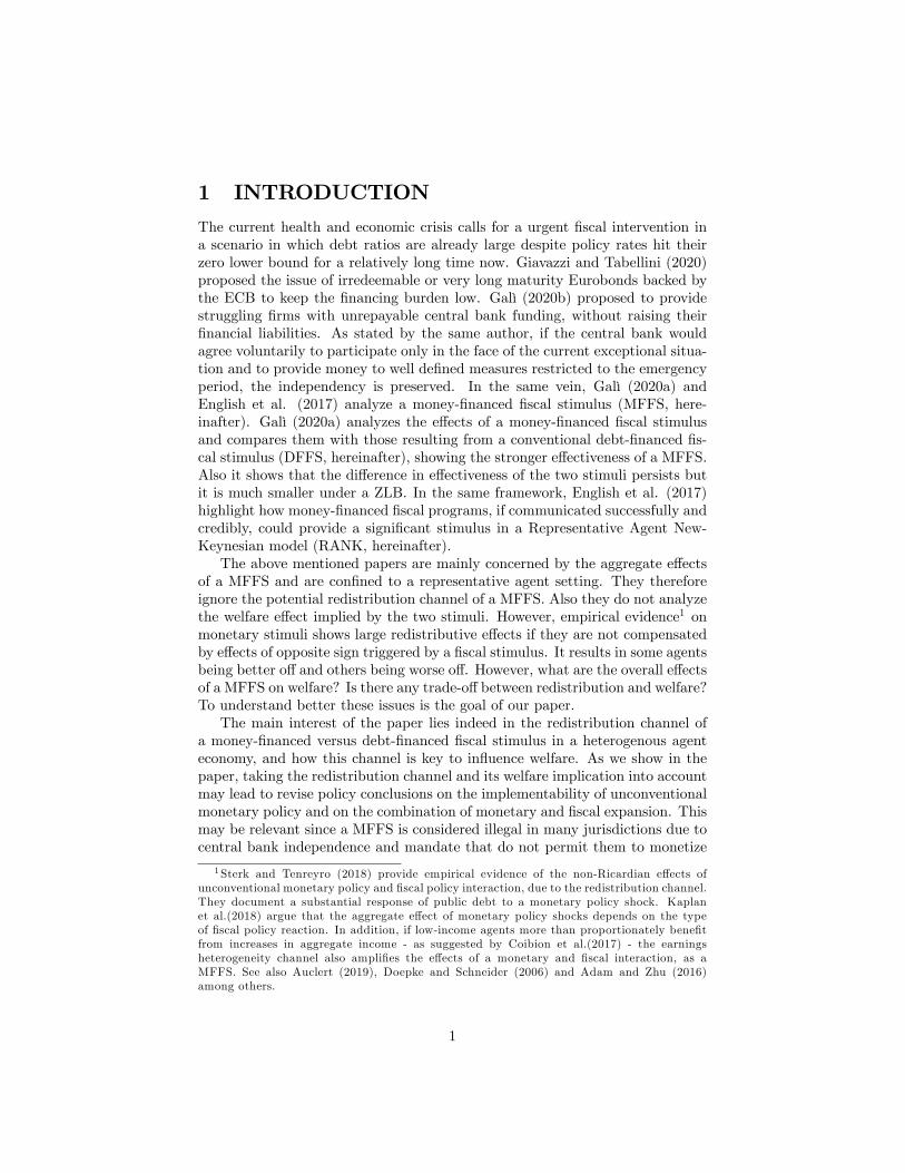
Consequently, the expansionary e¤ects of a MFFS are larger than those of aDFFS. Debt increases widely in the latter case, returning to its initial valueslowly, as guaranteed by �scal policy rule (through higher taxes). Under themoney �nancing scheme, the larger expansion in output and consumption leadsto an increase of in�ation, which reinforces the expansion in aggregate demandby lowering the real rate.As shown in Figure 3, if we compare the response of output and consumption

in a TANK model with the same responses in a RANK model - both a MFFSand a DFFS are more e¤ective in a TANK model, particularly a MFFS.

10

0 2 4 6 8 10 120

0.5

1

1.5

2Output ­ MFFS

RANKTANK

0 2 4 6 8 10 120

0.2

0.4

0.6

0.8

1Output ­ DFFS

0 2 4 6 8 10 120

0.2

0.4

0.6

0.8

1Consumption ­ MFFS

0 2 4 6 8 10 12

­0.2

­0.15

­0.1

­0.05

0

0.05Consumption ­ DFFS

RANKTANK

Fig. 3. Dynamic E¤ects of an Increase in Government Purchases: RepresentativeAgent (dotted lines) vs. Two-Agent (solid lines).

4.2.1 Multipliers

Next we discuss the sensitivity of some of the qualitative �ndings on the ef-fectiveness of �scal policy, particularly focusing on the share of borrowers. We�rstly compute the �scal multipliers of output and consumption associated toan increase in government purchases under the money-�nancing and the debt-�nancing regimes presented above. Then, in order to understand the role playedby the �nancial constraint, we evaluate the same multipliers under di¤erent val-ues of the steady state borrowing limit, �d:To di¤erentiate between the immediate impact of a change in �scal spending

and its long-run implications for the economy, we compute both the instanta-neous and the cumulative �scal multiplier, following Uhlig (2010).The Instantaneous Fiscal Multiplier (IFM, hereinafter) measures, in each

period, the percentage deviation of a generic variable Xt from its steady statein response to a change in government purchases that, on impact, amounts toone percent of the SS value of output. That is:

IFM(x) � xt

gT�G�Y

;8t � T

where xt = xt��x�x ; gT =

GT� �G�G

with t being the time index for the periodsfollowing the initial �scal shock in period T. �G and �Y are, respectively, thesteady state values of government spending and output. In particular, we willconsider the instantaneous multipliers associated to t = T; and we refer to themas Instantaneous Multipliers of x:As stressed in Uhlig (2010), policymakers cannot solely rely on the instanta-

neous multiplier since it can be misleading as it ignores the cumulated impact

11

of the initial �scal policy measure on the economy over time. Thus, in order tocapture the cumulative impact on the variable of interest of the �scal shock, weconsider also the cumulative �scal multiplier according to Uhlig (2010).The Cumulative Fiscal Multiplier (CFM, hereinafter) identi�es, in each pe-

riod, the discounted cumulative change of a variable xt measured in terms ofpercentage deviation from its steady state with respect to the discounted cu-mulative deviation of government spending from its steady state value. Thatis,

CFM(x) �Pt

s=T�R�(s�t)xs

�G�Y

Pts=T

�R�(s�t)gs;8t � T

where R being the steady state of the nominal interest rate used as discountrate.Figure 4 shows the IFM and CFM for consumption and output under money-

�nancing and debt-�nancing schemes, as � changes from 0:1 to 0:45: As ex-pected, consumption and output multipliers (both the impact and the cumu-lative ones) are higher under a MFFS than under a DFFS. The intuition isthe following one. A MFFS, having a crowding-in e¤ect on consumption ofboth agents, is associated to multipliers that are always higher than multipliersrelated to a DFFS.

0.1 0.15 0.2 0.25 0.3 0.35 0.4 0.450

2

4

6

Instanteneous Fiscal Multiplier of Consumption IFMC

MFFSDFFS=1

0.1 0.15 0.2 0.25 0.3 0.35 0.4 0.450

1

2

3

Cumulativ e Fiscal Multiplier of Consumption CFMC

0.1 0.15 0.2 0.25 0.3 0.35 0.4 0.45

2

4

6

Instantaneous Fiscal Multiplier of Output IFMY

0.1 0.15 0.2 0.25 0.3 0.35 0.4 0.451

1.5

2

2.5

3

3.5

Cumulativ e Fiscal Multiplier of Output CFMY

Fig. 4. Fiscal Multipliers. Value of dynamic instantaneous (left �gures) andcumulative (right �gures) �scal multipliers of consumption (top �gures) and output

(bottom �gures), as a function of the share of borrowers.

The impact and cumulative �scal multipliers of output related to a MFFS arealways greater than one, while those ones related to a DFFS need at least 20%of borrowers to be larger than one. Further, all multipliers considered increaseexponentially as the share of borrowers, �, increases, particularly the impactmultipliers. The multipliers of consumption, on the other hand, are larger than

12

� MFFS DFFSIFMC 24% 43%CFMC 29% 46%

Table 3: Share of borrowers associated to unitary �scal multipliers of consump-tion

one for values which depend on the type of multiplier that we analyze (instan-taneous or cumulative) and on the regime analyzed. Table (3) summarizes theresults.Finally, Figure 5 shows the CFM for three di¤erent values of the steady

state private debt: i) rule of thumb agents case (no borrowing, �d = 0); ii) netborrowers ( �d = 0:5); iii) no borrowing limit ( �d = 1), under the money-�nancingand the debt-�nancing scheme.Notice that, in all cases, �scal multipliers increase as �d increases. By relax-

ing the borrowing constraint in steady state, the borrower�s consumption canincrease more, and it generates higher �scal multipliers.

0.1 0.15 0.2 0.25 0.3 0.35

0.8

1

1.2

1.4

CFM Consumption ­ MFFS

d = 0d = 0.5d = 1

0.1 0.15 0.2 0.25 0.3 0.35

1.6

1.8

2

2.2CFM Output ­ MFFS

0.1 0.15 0.2 0.25 0.3 0.35

­0.1

0

0.1

0.2

0.3

CFM Consumption ­ DFFS

d = 0d = 0.5d = 1

0.1 0.15 0.2 0.25 0.3 0.35

0.9

1

1.1

1.2

CFM Output ­ DFFS

Fig. 5. Fiscal Multipliers. Value of dynamic cumulative �scal multipliers ofconsumption (left �gures) and output (right �gures) under a money-�nancing regime(top �gures) and a debt-�nancing regime (bottom �gures), as a function of the share

of borrowers.

To sum up, a MFFS implies always higher impact and cumulative �scal mul-tipliers than a DFFS. Under both �nancing schemes, �scal multipliers are anincreasing function of the share of borrowers and of the steady state borrowinglimit.

13

4.3 In a liquidity trap

Next we explore the e¤ectiveness of a money-�nanced �scal stimulus in stabiliz-ing the economy in face of a temporary adverse shock. The latter is assumed tobe large enough to prevent the central bank from fully stabilizing output, dueto a zero lower bound (ZLB) constraint on nominal interest rate. That MFFSis compared to a DFFS.Note that under the notation introduced above the ZLB constraint takes the

form 1 + it 1 1 for all t. The baseline experiment assumes that, "dt = � < 1for t = 0; 1; 2; :::T and "dt = 0 for t = T + 1; T + 2; ::In words, this describesa temporary adverse demand shock that brings the natural rate into negativeterritory up to period T: After period T;the shock vanishes and the naturalrate returns to its initial (positive) value. The shock is assumed to be fullyunanticipated but, once it is realized, the trajectory of "dt and the correspondingpolicy responses are known with certainty.In the case of a MFFS, the ZLB constraint can be incorporated formally

in the set of equilibrium conditions listed in Table (1) by replacing the saver�smoney demand with the complementarity slackness condition:

�1 + it � ��1s

� ��

��x� ms;t

cs;t

��� it1 + it

�= 0

for all t, where

1 + it 1 1is the ZLB constraint and

�

��x� ms;t

cs;t

��� it1 + it

1 0 (4)

represents the demand for real balances. As long as the nominal rate ispositive, (4) holds with equality (but it with inequality once the nominal ratereaches the ZLB and real balances overshoot their satiation level).By contrast, in the case of a DFFS, condition (3) must be replaced with

(1 + it � 1)�log

�1 + it1 + i

�� �� logEt

��t+1�

��= 0 for all t

together with

�log

�1 + it1 + i

�� �� logEt

��t+1�

��= 0 for t = T + 1; T + 2; ::

Thus, the zero in�ation target is assumed to be met once the shock vanishes;until that happens the nominal rate is assumed to be kept at the ZLB, i.e.1 + it = 1 for t = 0; 1; 2; :::TMoney-�nanced and debt-�nanced scenarios are analyzed next as a response

to the demand shock described above. We assume "dt = �0:065 and T = 6:

14

Thus, the experiment considered corresponds to an unanticipated drop of thenatural interest rate to �1% for �ve quarters, and a subsequent reversion backto the initial value of +1%:We start by considering the debt-�nanced government expenditure increase

(gt = 0:01, for t = 0; 1; :::; 5). The blue lines with diamonds in Figures 6 and7 show the economy�s responses to the adverse demand shock when the �scalauthority increases government expenditure by 1 per cent of steady state output�nancing the resulting de�cit through debt issuance and it lasts for the durationof the shock. The ZLB prevents the central bank from lowering the nominalrate to match the decline in the natural rate. As a result, we see that a debt-�nanced increase in government purchases is e¤ective at dampening the negativee¤ects of the adverse demand shock on output only in the �rst quarter. Notealso that real debt, and consequently taxes, increase considerably due to therise in real interest rates, which increases the government�s �nancial burden.Once the natural rate returns to its usual value, in�ation and the output gapare immediately stabilized at their zero target. The main reason for the lowe¤ectiveness of debt-�nanced government purchases in a liquidity trap (relativeto normal times) lies in the higher real interest rates relative to an identicalpolicy in "normal" times, combined with the lower expected in�ation induced,not only by the adverse demand shock, but also by the downward pressureexerted by borrowers.However, when the increase in government purchases (of the same size) is

money-�nanced (see red lines with circles), the impact on output and in�a-tion is substantial. A money-�nanced increase is now e¤ective at dampeningthe negative e¤ects of the adverse demand shock on output, after the secondquarter11 , and in�ation on impact - a �nding which complies with the resultsin normal times (see Fig.1). In other words, ceteris paribus a TANK modelrequires the adverse demand to be substantially larger to reproduce the resultsof a RANK model. The key di¤erence is again in the response of the aggregateconsumption. The greater e¤ectiveness of money-�nancing in the liquidity trapscenario can be traced to the associated lower real rate, due to the accumulatedliquidity resulting from the money-�nancing rule. These dynamics activate theredistribution channel described above.

11 In the �rst quarter, the absence of the Ricardian equivalence in a money-�nancing regimeand the decline of real wages, leads savers to decrease their labor supply on impact.

15

0 2 4 6 8 10­10

0

10output

MFFSDFFS

0 2 4 6 8 10­30

­20

­10

0

consumption

0 2 4 6 8 10­5

0

5

10real rate

0 2 4 6 8 10­10

­5

0

inflation

0 2 4 6 8 100

20

40

60

debt

0 2 4 6 8 100

1

2nominal rate

0 2 4 6 8 10­100

0

100

200money grow th

0 2 4 6 8 100

0.5

1

taxes

0 2 4 6 8 100

0.5

1gov ernment purchases

Fig. 6. Dynamic E¤ects of an Increase in Government Purchases in a LiquidityTrap: Debt vs. Money Financing.

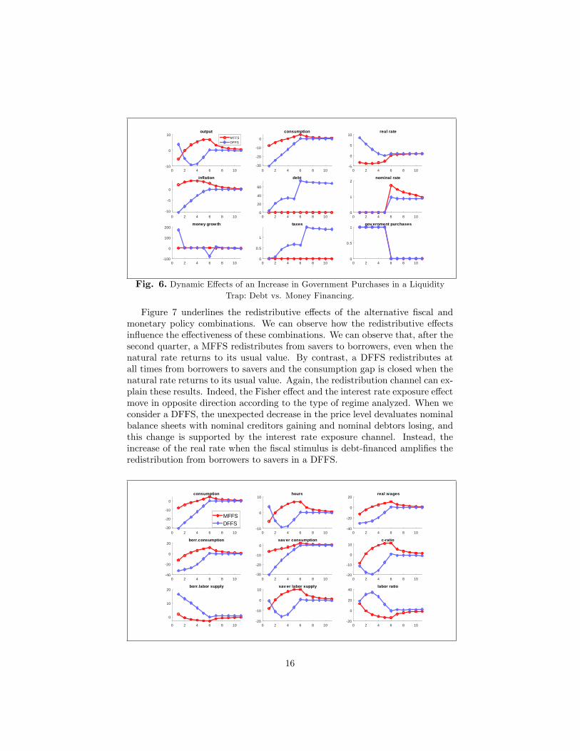
Figure 7 underlines the redistributive e¤ects of the alternative �scal andmonetary policy combinations. We can observe how the redistributive e¤ectsin�uence the e¤ectiveness of these combinations. We can observe that, after thesecond quarter, a MFFS redistributes from savers to borrowers, even when thenatural rate returns to its usual value. By contrast, a DFFS redistributes atall times from borrowers to savers and the consumption gap is closed when thenatural rate returns to its usual value. Again, the redistribution channel can ex-plain these results. Indeed, the Fisher e¤ect and the interest rate exposure e¤ectmove in opposite direction according to the type of regime analyzed. When weconsider a DFFS, the unexpected decrease in the price level devaluates nominalbalance sheets with nominal creditors gaining and nominal debtors losing, andthis change is supported by the interest rate exposure channel. Instead, theincrease of the real rate when the �scal stimulus is debt-�nanced ampli�es theredistribution from borrowers to savers in a DFFS.

0 2 4 6 8 10­30

­20

­10

0

consumption

0 2 4 6 8 10­10

0

10hours

0 2 4 6 8 10­40

­20

0

20real wages

0 2 4 6 8 10­40

­20

0

20borr.consumption

0 2 4 6 8 10­30

­20

­10

0sav er consumption

0 2 4 6 8 10­20

­10

0

10c­ratio

MFFSDFFS

0 2 4 6 8 10

0

10

20borr.labor supply

0 2 4 6 8 10­20

­10

0

10sav er labor supply

0 2 4 6 8 10­20

0

20

40labor ratio

16

Fig. 7. Dynamic e¤ects of an Increase in Government Purchases in a LiquidityTrap: Debt vs. Money Financing.

However, as shown in Figure 8, under a money-�nancing regime, the presenceof borrowers exerts an upward pressure on in�ation that is absent in a RANKmodel. Hence, the redistribution under a money-�nancing regime is explained bythe Fisher channel. By contrast, under a debt-�nancing regime, the magnitudeof the redistribution channel is solely explained by borrower�s labor supply.The absence of borrowers in a RANK model makes the economy to enter in arecession from the �rst quarter.

0 2 4 6 8 10 12­10

­5

0

5

10Output ­ MFFS

RANKTANK

0 2 4 6 8 10 12­10

­5

0

5Output ­ DFFS

0 2 4 6 8 10 12­20

­15

­10

­5

0

5Consumption ­ MFFS

2 4 6 8 10­30

­20

­10

0Consumption ­ DFFS

RANKTANK

Fig. 8. Dynamic E¤ects of an Increase in Government Purchases in a LiquidityTrap: Representative Agent vs. Two-Agent Model.

We can therefore summarized the result as follows. A liquidity trap scenarioampli�es the di¤erences between MFFS and DFFS. A MFFS in a TANK modelis e¤ective at dampening the negative e¤ect of the adverse demand shock. Thisis not valid in a RANK model (see Galì, 2020).

5 WELFARE

This section provides a welfare evaluation of the two alternative �nancing regimesof a government expenditure increase, the money-�nancing regime and the debt-�nancing. A formal evaluation of the performance of a MFFS with respect toa DFFS requires the use of some quantitative criterion. Following the semi-nal work of Woodford (2002) and Benigno and Woodford (2003), we adopt awelfare-based criterion, relying on a second-order approximation of the utilitylosses due to the deviations from the e¢ cient allocation. In particular, in linewith Ferrero et al. (2018), we derive the welfare-based loss function of theaverage per-period utility functions of borrowers and savers in an utilitarianperspective, by weighting the utility of each type of agent according to their

17

share in the population. Further, we assume that the policy maker discountsthe future by using savers�discount factor. The second order approximationyields the following welfare-loss function:12

fWt '1

2E0�

ts

1Xt=0

� xex2t + Cec2t + ��2t �+ t:i:p: (5)

where welfare losses are expressed in terms of the equivalent permanent con-sumption, measured as a fraction of steady state consumption. Notice that, asin Ferrero et al. (2018), the loss function not only depends on output gap andin�ation but also on the consumption gap between borrowers�consumption andsavers�one. The term ect = bcbt�bcst is indeed the gap between borrowers�consump-tion and savers�one; ext = yt�yEfft measures the output gap between the actualoutput and the e¢ cient equilibrium output13 and �t measures the in�ation gapbetween the actual in�ation and the long run rate, set equal to 1 in gross terms.Since all terms are squared terms, the larger the gaps the higher will be the

implied welfare losses. The coe¢ cients x = (� + �) ; C =�(1��)�('+�)

�1+�+'1+'

�and � = �P represent the weights attached respectively to output gap, con-sumption gap and in�ation gap.The average welfare loss per period is thus given by the following linear

combination of the variances of output gap, in�ation and consumption gap:

L = ('+ �)

2[ xvar(ext) + Cvar (ect) + �var (�t)] : (6)

Given our particular policy regimes (MFFS versus DFFS) and the calibrationof the model�s parameters, one can determine the implied variance of in�ation,output gap, consumption gap and the corresponding welfare losses associatedwith each policy regime.Table 4 displays some statistics for the three alternative regimes: i) a MFFS;

2) a DFFS with a Central Bank implementing a standard Taylor rule with �� =1:5; iii) a DFFS with a Central Bank implementing a strict in�ation targetingrule, �t = 0: The remaining parameters are calibrated at their baseline valuesas in the rest of the paper. For each policy regime, Table 4 shows the impliedstandard deviations of output gap, in�ation and consumption gap, expressedin percent terms, as well as the welfare losses resulting from the associateddeviations from the e¢ cient allocation, expressed as a fraction of steady stateconsumption. The same statistics are shown for the baseline model and for theRANK model. In the latter case, the average welfare loss function becomes:

LRANK =1

2[ xvar(ext) + �var (�t)] (7)

Several results stand out. First, in a way consistent with the analysis presentedin Section 3 on IRFs and consumption and income multipliers, a MFFS generates12Technical details on the derivation of the objective function are left to the Appendix.13This is true when yEfft = 1+'

1+�at is the e¢ cient output under the assumption that yt =

Atnt and At is an exogenous productivity shock.

18

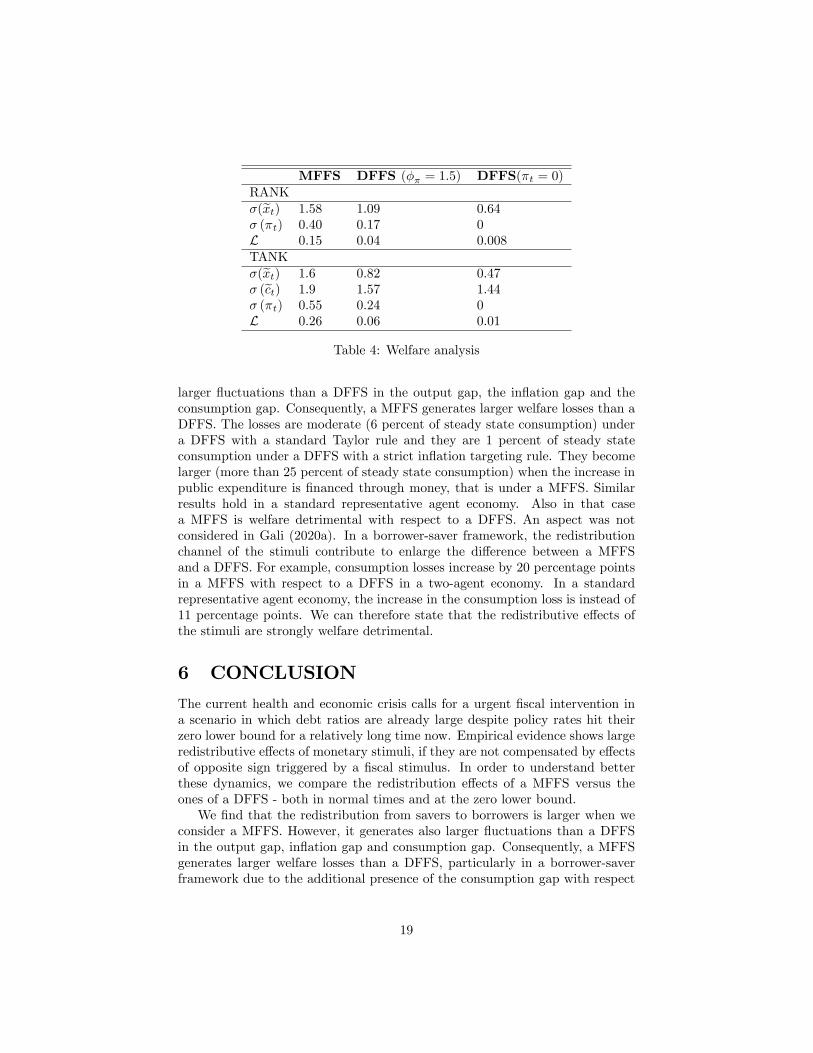
MFFS DFFS (�� = 1:5) DFFS(�t = 0)RANK�(ext) 1:58 1:09 0:64� (�t) 0:40 0:17 0L 0:15 0:04 0:008TANK�(ext) 1:6 0:82 0:47� (ect) 1:9 1:57 1:44� (�t) 0:55 0:24 0L 0:26 0:06 0:01

Table 4: Welfare analysis

larger �uctuations than a DFFS in the output gap, the in�ation gap and theconsumption gap. Consequently, a MFFS generates larger welfare losses than aDFFS. The losses are moderate (6 percent of steady state consumption) undera DFFS with a standard Taylor rule and they are 1 percent of steady stateconsumption under a DFFS with a strict in�ation targeting rule. They becomelarger (more than 25 percent of steady state consumption) when the increase inpublic expenditure is �nanced through money, that is under a MFFS. Similarresults hold in a standard representative agent economy. Also in that casea MFFS is welfare detrimental with respect to a DFFS. An aspect was notconsidered in Gali (2020a). In a borrower-saver framework, the redistributionchannel of the stimuli contribute to enlarge the di¤erence between a MFFSand a DFFS. For example, consumption losses increase by 20 percentage pointsin a MFFS with respect to a DFFS in a two-agent economy. In a standardrepresentative agent economy, the increase in the consumption loss is instead of11 percentage points. We can therefore state that the redistributive e¤ects ofthe stimuli are strongly welfare detrimental.

6 CONCLUSION

The current health and economic crisis calls for a urgent �scal intervention ina scenario in which debt ratios are already large despite policy rates hit theirzero lower bound for a relatively long time now. Empirical evidence shows largeredistributive e¤ects of monetary stimuli, if they are not compensated by e¤ectsof opposite sign triggered by a �scal stimulus. In order to understand betterthese dynamics, we compare the redistribution e¤ects of a MFFS versus theones of a DFFS - both in normal times and at the zero lower bound.We �nd that the redistribution from savers to borrowers is larger when we

consider a MFFS. However, it generates also larger �uctuations than a DFFSin the output gap, in�ation gap and consumption gap. Consequently, a MFFSgenerates larger welfare losses than a DFFS, particularly in a borrower-saverframework due to the additional presence of the consumption gap with respect

19

to a RANK model. To sum up, the redistributive e¤ects are welfare detrimental.This the reason why only a borrower-saver framework can highlight the trade-o¤faced by a government to �nance a �scal stimulus by money creation, if it isnot forbidden by the legislation. A MFFS has larger redistributive e¤ects thana DFFS but it also implies a larger welfare loss due to the redistributive e¤ectitself. A corollary of this result is that a MFFS implies always higher impactand cumulative �scal multipliers than a DFFS. Under both �nancing schemes,�scal multipliers are an increasing function of the share of borrowers and of thesteady state borrowing limit.In addition, a liquidity trap scenario ampli�es the di¤erences between MFFS

and DFFS. A MFFS is e¤ective at dampening the negative e¤ect of the adversedemand shock in a TANK model. This is not valid in a RANK model (see Galì,2020a).Debortoli and Galì (2017) show that TANK models can provide a good

and tractable approximation of the HANK models. They show that a TANKmodel approximates well, both quantitatively and qualitatively the dynamics ofan HANK model in response to aggregate shocks. For this reason we believethat our results will be robust to the introduction of a more structured HANKmodel, even though studying the e¤ects of this stimulus by using the latestgeneration of HANK models is also part of our research agenda. Considering anon-Walrasian labor market or investigating the e¤ects of a MFFS in a mediumscale model, as well as considering the possibility of relaxing the assumption ofrational expectations are all important research questions that are left to futureresearch.

20

References

[1] Adam, Klaus and Junyi Zhu (2016). Price Level Changes and the Redistri-bution of Nominal Wealth Across the Euro Area, Journal of the EuropeanEconomic Association, 14(4), 871-906.

[2] Annicchiarico, Barbara, Nicola Giammarioli, and Alessandro Piergallini(2012). Budgetary Policies in a DSGEModel with Finite Horizons, Researchin Economics, 66(2).

[3] Auclert, Adrien. (2019). Monetary Policy and the Redistribution Channel,American Economic Review, 109, 2333-2367.

[4] Benigno, Pierpaolo and Michael Woodford (2003). Optimal Monetary andFiscal Policy: A Linear-Quadratic Approach in M. Gertler and K. Rogo¤,eds., NBER Macroeconomics Annual 2003, Cambridge (US), MIT Press,18, 271-333.

[5] Bilbiie, Florin.O.(2008). Limited asset market participation, monetary pol-icy, and (inverted) aggregate demand logic, Journal of Economic Theory,140(1), 162-196.

[6] Bilbiie, Florin O., Tommaso Monacelli, and Roberto Perotti (2013). PublicDebt and Redistribution with Borrowing Constraints, Economic Journal,123, 64-98.

[7] Coibion, Olivier, Yuriy Gorodnichenko, Lorenz Kueng, and John Silvia(2017). Innocent Bystanders? Monetary policy and Inequality in the U.S.,Journal of Monetary Economics, 88, 70-89.

[8] Debortoli, Davide, and Jordi Galí (2017). Monetary policy with hetero-geneous agents: Insights from TANK models, Economics Working Papers1686, Department of Economics and Business, Universitat Pompeu Fabra.

[9] Doepke, Matthias, and Martin Schneider (2006). Aggregate Implicationsof Wealth Redistribution: The Case of In�ation, Journal of the EuropeanEconomic Association, 4, 493-502.

[10] Eggertsson, Gauti B, and Paul Krugman (2012). Debt, Deleveraging, andthe Liquidity Trap: a Fisher-Minsky-Koo Approach, The Quarterly Journalof Economics, 127(3), 1469-1513.

[11] English William B., Christopher J. Erceg, and David Lopez-Salido. (2017).Money-Financed Fiscal Programs: A Cautionary Tale, FEDS Working Pa-per No. 2017-060.

[12] Ferrero, Andrea, Richard Harrison and Ben Nelson (2018). Concerted ef-forts? Monetary policy and macro-prudential tools, Bank of England work-ing papers 727.

21

[13] Giavazzi, Francesco and Guido Tabellini (2020). Covid Perpetual Eu-robonds: Jointly guaranteed and supported by the ECB, VoxEu.org, 24March 2020.

[14] Galì, Jordi (2020a). The e¤ects of a money-�nanced �scal stimulus, Journalof Monetary Economics, 115, 1-19.

[15] Galì, Jordi (2020b). Helicopter money. The time is now, VoxEu.org, 17March 2020.

[16] Galì, Jordi, David Lopez-Salido, and Javier Vallés (2007). Understandingthe E¤ects of Government Spending on Consumption, Journal of the Eu-ropean Economic Association, 5(1), 227-270.

[17] Iacoviello, Matteo (2005). House Prices, Borrowing Constraints and Mon-etary Policy in the Business Cycle, American Economic Review, 95(3),739-764.

[18] Kaplan, Greg, Benjamin Moll, and Giovanni L.Violante (2018). MonetaryPolicy According to HANK, American Economic Review, 108(3), 697-743.

[19] Kiyotaki, Nobuhiro, and John Moore (1997). Credit cycles, Journal of Po-litical Economy, 105, 211-248.

[20] Mankiw, N.Gregory (2000). The Savers-Spenders Theory of Fiscal Policy,American Economic Review, 90(2), 120-125.

[21] Monacelli, Tommaso (2009). New Keynesian models, durable goods, andcollateral constraints, Journal of Monetary Economics, 56(2), 242-254.

[22] Monacelli, Tommaso, and Roberto Perotti (2011). Redistribution and theMultiplier, IMF Economic Review, 59(4), 630-651.

[23] Sterk, Vincent, and Silvana Tenreyro. (2018). The Transmission of Mon-etary Policy Operations through Redistributions and Durable Purchases,Journal of Monetary Economics, 99, 124-137.

[24] Uhlig, Harald. (2010). Some Fiscal Calculus, American Economic Review,100(2), 30-34.

[25] Woodford, Michael (2002). In�ation Stabilization and Welfare, The B.E.Journal of Macroeconomics, 2(1), 1-53.

22

A SENSITIVITY ANALYSIS

Under debt �nancing, monetary policy is assumed to pursue an in�ation tar-geting mandate implying Equation (3) :However, a key parameter in these com-parisons is the coe¢ cient in the interest rate rule (�� = 1:5 is our benchmark) :Next, we discuss the sensitivity of the redistribution channel of a DFFS regard-ing that coe¢ cient.We consider two alternative values with respect to our benchmark: i) �� =

5;ii) �� !1, as in Galì (2019). Fig. 9 displays the response over time of output,in�ation, debt and other macroeconomic variables of interest to an exogenousincrease in government purchases, under the baseline calibration. The red lineswith circles display the responses under the money-�nancing scheme, while theblue lines with diamonds show the response under the debt-�nancing schemewhen �� = 1:5; the dotted blue lines when �� = 5 and the dashed blue lineswhen �� ! 1;or in other words, �t = 0: For debt and taxes, we display thepercent response of, respectively, real debt and taxes.

0 2 4 6 8 100

1

2output

MFFSDFFS (Pai = 0)DFFS (phipai = 1.5)DFFS (phipai = 5)

0 2 4 6 8 10­0.5

0

0.5

1consumption

0 2 4 6 8 10­0.2

0

0.2

0.4

real rate

0 2 4 6 8 100

0.2

0.4

inflation

0 2 4 6 8 100

5

10debt

0 2 4 6 8 100

0.2

0.4

nominal rate

0 2 4 6 8 10

­50

0

50money grow th

0 2 4 6 8 100

0.1

0.2taxes

0 2 4 6 8 100

0.5

1gov ernment purchases

Fig. 9. Redistribution channel: The Role of IT rule.

Fig. 10 displays the response over time of the disaggregated consumptionand disaggregated labor supply as well as the consumption ratio (Cb=Cs) andlabor ratio (Nb=Ns) to an exogenous increase in government purchases. Thehigher the coe¢ cient in the interest rate rule, the higher is the increase in nom-inal rates. It creates a consumption crowding-in solely when �� = 1:5 (and ina money-�nancing regime). The higher ��; the higher the crowding out e¤ecton aggregate consumption will be (and the money demand collapse). Figure10 underlines the redistributive e¤ects. The higher ��; the lower redistributionchannel is, also if whatever combination we analyze it brings about a redistri-bution from savers to borrowers. However, an IT rule with �� ! 1 is ableto redistribute 30% of what an IT rule with �� = 1:5 is able to do, because ofthe interest rate exposure e¤ect. The latter is increasing with the size of ��;

23

but it redistributes from borrowers to savers. In other words, the higher ��;the higher is the ability of the interest rate exposure e¤ect of compensating theFisher e¤ect and minimizing it.

0 5 10

­0.5

0

0.5

1consumption

0 5 10­1

0

1

2

3

4borr.consumption

0 5 10­1

­0.5

0

0.5sav er consumption

0 5 100

1

2

3c­ratio

0 5 100

0.5

1

1.5

2hours

0 5 10­0.6

­0.4

­0.2

0

0.2

0.4borr.labor supply

0 5 100

1

2

3sav er labor supply

0 5 10­4

­3

­2

­1

0

1labor ratio

MFFSDFFS (Pai = 0)DFFS (phipai = 1.5)DFFS (phipai = 5)

Fig. 10. Redistribution channel: The Role of IT rule.

This is the reason why, as shown in Figure 11, the interest rate exposuree¤ect is perfectly able to compensate the Fisher channel when �� !1:

0 5 100

0.5

1

1.5

2Output ­ MFFS

RANKTANK

0 5 100

0.2

0.4

0.6

0.8

1Output ­ DFFS(phipai = 1.5)

RANKTANK

0 5 100

0.2

0.4

0.6

0.8Output ­ DFFS(phipai = 5)

RANKTANK

0 5 100

0.2

0.4

0.6Output ­ DFFS(Pai = 0)

0 5 100

0.2

0.4

0.6

0.8

1Consumption ­ MFFS

0 5 10

­0.2

­0.15

­0.1

­0.05

0

Consumption ­ DFFS(phipai = 1.5)

0 5 10­0.4

­0.3

­0.2

­0.1

0Consumption ­ DFFS(phipai = 5)

0 5 10­0.6

­0.4

­0.2

0Consumption ­ DFFS(Pai = 0)

RANKTANK

Fig. 11. RANK vs TANK: The role of IT rule

B WELFARE DERIVATIONS

B.1 Derivation of the E¢ cient Steady State

Let us to consider the steady state e¢ cient equilibrium. It establishes theconditions under which a zero in�ation (� = 1) steady state is e¢ cient. Indeed,

24

it measures the subsidy/tax needed in the decentralized equilibrium in order toobtain the e¢ ciency of the steady state allocation. First of all, we consider aSocial Planner that maximizes the following welfare function in steady state

U = e�U �cb; nb�+ �1� e��U (cs; ns) (8)

where e� is a Pareto weight e� 2 [0; 1] and where U �cj ; nj� is the per-period utilityfunction of type j = fb; sg household. As in the numerical analysis, we assumethat real balances have a negligible weight in utility relative to consumption oremployment, so that they do not a¤ect welfare results.14 The Social Plannermaximizes the welfare function under the constraints given by the productionfunction,

y = n; (9)

the resource constraint,c+ g = y; (10)

and the aggregations of consumption and labor given respectively by:

c = �cb + (1� �) ch; (11)

n = �nb + (1� �)ns: (12)

Combining the constraints in a unique constraint, we get

�cb + (1� �) ch + g = �nb + (1� �)ns: (13)

The Lagrangian implied is

U = e�U �cb; nb�+�1� e��U (cs; ns)��1 ��cb + (1� �) ch + g � �nb � (1� �)ns� :(14)

Taking the �rst order conditions with respect to cb; nb; cs; ns; we gete�U bc = �1�;e�U bn = �1�;�1� e��Usc = ��1 (1� �) ; and�1� e��Usn = ��1 (1� �) :

Notice that FOCs imply

U bc = U bc

U bn = U bn

and that

cb = cs = c; and

nb = ns = n:14We assume that �! 0 . We do not want that welfare results on MFFS are driven by the

presence of real balances in the utility function. We adopt a conservative assumption.

25

Hence,U bnU bc

=UsnUsc

= � yn= �1

that comes from y = n:It can be shown that the standard subsidy applies. Indeed, in the decentral-

ized equilibrium of the labor market, the labor supply choices are given by thefollowing equations

w = ��bU bnU bc

w = ��sUsnUsc

while the labor demand is given according to

w = mc =�

�� 1 :

The equilibrium in the labor market implies

�

�� 1 = �

���b

U bnU bc

�+ (1� �)

���s

UsnUsc

�:

And, if as we have assumed in our model �b = �s = 1; then

� �

�� 1 = �

�U bnU bc

�+ (1� �)

��sUsnUsc

�:

To get the e¢ cient equilibrium, it must hold that ���1 = 1. Thus, a standard

employment subsidy is su¢ cient to get the result, so that in the decentralizedequilibrium, the labor demand becomes

w (1� �L) = mc =�� 1�

: (15)

It implies that the decentralized equilibrium will be equal to the e¢ cient one if:

�1 = � �� 1� (1� �L)

= �

�U bnU bc

�+ (1� �)

��sUsnUsc

�implying

1 = � �� 1� (1� �L)

and thus, solving for �L we get the optimal subsidy,

�L = 1��� 1�

=1

�: (16)

26

B.2 Derivation of the Welfare Based Loss Function

We can now move to the second order approximation of the household utilityfunction

W0 = E0

1Xt=0

�tsUt

!(17)

whereUt = e�U �cbt ; nbt�+ �1� e��U (cst ; nst ) (18)

Following Woodford (2002), we take the second order approximation aroundthe e¢ cient steady state, ignoring terms of order three and higher, and alsoexogenous terms, so that

Ut � U ' e� �U bc �cbt � cb�+ 12U bcc �cbt � cb�2�+

+�1� e���Usc (cst � cs) + 12Uscc (cst � cs)2

�+e� �U bn �nbt � nb�+ 12U bnn �nbt � nb�2

�+

+�1� e���Usn (nst � ns) + 12Usnn (nst � ns)2

�Now, factoring out the marginal utility of consumption and labor for each typeof household:

Ut � U ' e�U bc ��cbt � cb�+ 12 U bccU bc �cbt � cb�2�+�1� e��Usc �(cst � cs) + 12 UsccUsc (cst � cs)2

�+e�U bn ��nbt � nb�+ 12 U bnnU bn �nbt � nb�2

�+�1� e��Usn �(nst � ns) + 12 UsnnUsn (nst � ns)

2

�:

By using the FOCs of the e¢ cient steady state, that is for

e�U bc = �1�e�U bn = �1��1� e��Usc = ��1 (1� �)�1� e��Usn = ��1 (1� �)

it becomes

Ut � U ' ��1

��cbt � cb

�+1

2

U bccU bc

�cbt � cb

�2�+ (1� �)�1

�(cst � cs) +

1

2

UsccUsc

(cst � cs)2

����1

��nbt � nb

�+1

2

U bnnU bn

�nbt � nb

�2�� (1� �)�1 �(nst � ns) + 12 UsnnUsn (nst � ns)2

�:

27

Given the preferences in the period utility of each household

U bccU bc

=UsccUsc

= � �C

U bnnU bn

=UsnnUsn

='

n;

substituting above and collecting �rst order terms, we obtain:

Ut � U ' �1���cbt � cb

�+ (1� �) (cst � cs)

���1

���nbt � nb

�+ (1� �) (nst � ns)

���1

1

2

�

C

h��cbt � cb

�2+ (1� �) (cst � cs)

2i

��11

2

'

n

h��nbt � nb

�2+ (1� �) (nst � ns)

2i:

By considering aggregate consumption, ct = �cbt+(1� �) cst ; and taking the �rstorder approximation around the e¢ cient steady state, the previous objectivefunction can be rewritten as

Ut � U ' �1 (ct � c)��1

���nbt � nb

�+ (1� �) (nst � ns)

���1

1

2

�

C

h��cbt � cb

�2+ (1� �) (cst � cs)

2i

��11

2

'

n

h��nbt � nb

�2+ (1� �) (nst � ns)

2i:

Given the resource constraint implied by the Rotemberg model, the secondorder approximation of that constraint implies

C

�bct + 12bc2t� = y

�byt + 12by2t�� �P

2y�2t

Then, under the e¢ cient steady state15 ,

ct � c = bct + 12bc2t = byt + 12by2t � �P

2y�2t

the welfare function becomes

Ut � U ' �1y

�byt + 12by2t � �P

2y�2t

���1

���nbt � nb

�+ (1� �) (nst � ns)

���1

1

2

�

C

h��cbt � cb

�2+ (1� �) (cst � cs)

2i

��11

2

'

n

h��nbt � nb

�2+ (1� �) (nst � ns)

2i;

15As in Benigno and Woodford (2003), we can omit exogenous terms like gt. Also noticethat its steady state is zero in the e¢ cient steady state.

28

from

nbt � nb = nb�bnbt + 12 �bnbt�2

�= n

�bnbt + 12 �bnbt�2�

nst � ns = ns�bnst + 12 (bnst )2

�= n

�bnst + 12 (bnst )2�

and then

Ut � U ' �1y

�byt + 12by2t � �P

2�2t

���1

��n

�bnbt + 12 �bnbt�2�+ (1� �)n

�bnst + 12 (bnst )2��

��11

2

�

C

h��cbt � cb

�2+ (1� �) (cst � cs)

2i

��11

2

'

n

h��nbt � nb

�2+ (1� �) (nst � ns)

2i

or

�1 (Ut � U) ' y

��byt + 12by2t�� �P

2�2t

��n��bnbt + (1� �) bnst�� 12n h� �bnbt�2 + (1� �) (bnst )2i

�12

�

c

h��cbt � cb

�2+ (1� �) (cst � cs)

2i

�12

'

n

h��nbt � nb

�2+ (1� �) (nst � ns)

2i

Knowing that in steady state cb = cs = c = y and nb = ns = n = y andfrom �

cbt � cb�2

=�cb�2 �bcbt�2 = (c)2 �bcbt�2

(cst � cs)2= (cs)

2(bcst )2 = (c)2 (bcst )2�

nbt � nb�2

=�nb�2 �bnbt�2 = (n)2 �bnbt�2

(nst � ns)2= (ns)

2(bnst )2 = (n)2 (bnst )2

Substituting and rearranging

�1 (Ut � U)y

'�byt + 1

2by2t�� �P

2�2t

���bnbt + (1� �) bnst�� 12 h� �bnbt�2 + (1� �) (bnst )2i

�12�h��bcbt�2 + (1� �) (y)2 (bcst )2i

�12'h��bnbt�2 + (1� �) (bnst )2i :

29

Further, from the production function we know that

byt = bnt = �bnbt + (1� �) bnstand therefore, simplifying and collecting terms, the objective function is

�1 (Ut � U)y

' 1

2by2t � �P

2�2t �

1

2�h��bcbt�2 + (1� �) (bcst )2i

�12(1 + ')

h��bnbt�2 + (1� �) (bnst )2i :

Notice that, at this point, the welfare-based loss function is fully quadratic. Fol-lowing Ferrero et al.(2018), we rewrite it to obtain terms with a more meaningfuleconomic interpretation. Hence, we combine terms in output and consumption,as follows

�1 (Ut � U)y

' �12

n�h��bcbt�2 + (1� �) (bcst )2i� by2to

�12(1 + ')

h��bnbt�2 + (1� �) (bnst )2i� �P

2�2t�

Now we rewrite the objective function adding and subtracting 12 (� + ') by2t

�1 (Ut � U)y

' �12

n�h��bcbt�2 + (1� �) (bcst )2i� by2to� 12 (1 + ') h� �bnbt�2 + (1� �) (bnst )2i

+1

2(� + ') by2t � 12 (� + ') by2t � �P

2�2t + t:i:p:

where t:i:p collects all terms independent of policy. We can put 12�by2t into the

consumption terms and 12 (1 + ') by2t into the labor terms

eUt ' �12

��h��bcbt�2 + (1� �) (bcst )2i+ �by2t + 12 (1 + ') h� �bnbt�2 + (1� �) (bnst )2 � by2t i� (� + ') by2t�

�+

��P2�2t �

�P2�2t + t:i:p:

where eUt = �1(Ut�U)y :

Now notice that

��bcbt�2 + (1� �) (y)2 (bcst )2 � by2t = �

��bcbt�2 � by2t �+ (1� �)�(bcst )2 � by2t �using again the resource constraint to replace the di¤erences between each type�sconsumption and output, we can rewrite

��bcbt�2 + (1� �) (y)2 (bcst )2 � by2t = � (1� �)

�bcbt � bcst�2Then from the labor supply conditions,

wt =�nbt�' �

cbt��

wt = (nst )'(cst )

�

30

then �nbt�' �

cbt��= (nst )

'(cst )

�;

and also from

wtnbt =

�nbt�1+' �

cbt��

wtnst = (nst )

1+'(cst )

�

then, the �rst order approximation gives us:

(1 + ') bnbt + �bcbt = wt + bnbt(1 + ') bnst + �bcst = wt + bnst

Then, by aggregating

��wt + bnbt�+ (1� �) (wt + bnst ) = wt + bnt = (1 + ') bnt + �bct

��wt + bnbt�+ (1� �) (wt + bnst ) = wt + bnt = (1 + ') bnt + �byt

and given that bnt = �bnbt + (1� �) bnst ;wt + bnt = (1 + ') bnt + �byt = (1 + ') ��bnbt + (1� �) bnst�+ �byt

consequently,

(1 + ')��bnbt + (1� �) bnst�+ �byt = (1 + ') bnbt + �bcbt

and by collecting terms in bnbtbnbt = bnst � �

1 + ' (1� �)�bcbt � byt�

and bnst = �bnt � �bnbt�1� �and by substituting the last one into the previous one and solving for bnbt ;

bnbt = bnt � �

1 + '

�bcbt � byt� = byt � �

1 + '

�bcbt � byt�Similarly, we �nd bnst = byt � �

1 + '(bcst � byt)

Then, using the �rst order approximation of the resource constraint we canrewrite

bnbt = byt � �

1 + '(1� �)

�bcbt � bcst�bnst = byt + �

1 + '��bcbt � bcst�

31

substituting everything into the objective function

eUt ' �12

8>>>>><>>>>>:

�� (1� �)�bcbt � bcst�2+

+ 12 (1 + ')

264 ��byt � �

1+' (1� �)�bcbt � bcst��2+

+(1� �)�byt + �

1+'��bcbt � bcst��2 � by2t

375� (� + ') by2t � �P

2 �2t + t:i:p:

9>>>>>=>>>>>;Let us to consider only the terms in the squared brackets"�

�byt � �

1 + '(1� �)

�bcbt � bcst��2 + (1� �)�byt + �

1 + '��bcbt � bcst��2 � by2t

#and expand the two squared terms

�

by2t + � �

1 + '(1� �)

�bcbt � bcst��2 � 2 �

1 + '(1� �)

�bcbt � bcst� by2t!+

+(1� �) by2t + � �

1 + '��bcbt � bcst��2 + 2 �

1 + '��bcbt � bcst� by2t

!� by2t :

By simplifying, we obtain:

by2t + � (1� �) (1� �) � �

1 + '

�bcbt � bcst��2 + (1� �)��� �

1 + '

�bcbt � bcst��2 � by2t= � (1� �)

��

1 + '

�bcbt � bcst��2and by substituting in the objective function and by collecting terms

eUt ' �12

�('+ �) by2t + � (1� �)��1 + � + '1 + '

��bcbt � bcst�2�� �P2�2t + t:i:p:

where t:i:p: indicates terms independent from policy. In particular, with aproduction function where yt = Atnt and At representing an exogenous TFPshocks, the implied welfare function would be

eUt ' � ('+ �)2

E0�ts

1Xt=0

�('+ �) ex2t + � (1� �)��1 + � + '1 + '

�ec2t + �P�2t�+t:i:p:(19)

where, we de�ne ect = bcbt � bcst as the consumption gap we have de�ned ext =byt � yEfft , with yEfft = 1+��+�at and at = ln (At=A) the log-deviation of the

TFP from its steady state. Otherwise, in the absence of this shock, as in ourparticular model economy, ext = byt: Multiplying everything by -1, the Lossfunction becomes

fWt '1

2E0�

ts

1Xt=0

�('+ �) ex2t + � (1� �)��1 + � + '1 + '

�ec2t + �P�2t�+ t:i:p:(20)

32

Notice that as in Ferrero et al (2018) the welfare function depends, not onlyon standard output gap and in�ation but also on the consumption gap betweenborrower and saver consumption. Since all terms are squared terms, the largerthe gaps the higher will be the welfare loss. To interpret our numerical results intable (4) ; it is indeed important to analyze the role played by the redistributivechannel of each stimulus in a¤ecting not only in�ation and output but also theconsumption gap, which is indeed crucial to explain the results.

33