IRRIIS Integrated Risk Reduction of Information-based ...

IST Project N° 027568

Project co-funded by the European Commission within the Sixth Framework

Programme (2002-2006)

Integrated Project

IRRIIS

Integrated Risk Reduction of Information-based

Infrastructure Systems

Deliverable D 2.1.1

Intermediate report on LCCI topology and

vulnerability assessment

Due date of deliverable: 31 July 2006

Actual submission date: 31 July 2006

Revision 1.0

Technical University Dresden

Dissemination Level

PU Public

Start date of project: 01 February 2006 Duration: 3 years

D 2.1.1: Intermediate report on LCCI topology and vulnerability assessment

2

Author(s) Ester Ciancamerla (ENEA)

Niels von Festenberg (TUD)

Pekka Koponen (VTT)

Gwendal Le Grand (ENST)

Michele Minichino (ENEA)

Peter Popov (CU)

Vittorio Rosato (ENEA)

Kizito O. Salato (CU)

Ingve Simonsen (TUD)

Contributor(s) Sandro Bologna (ENEA)

Dirk Helbing (TUD)

Karsten Peters (TUD)

ENEA

Siemens

Work package WP 2.1 : “LCCI topology analysis: data and scenario understanding”

Task(s) Task 2.1.1: “Collection, modelling and analysis of LCCI topology data”

Quality Manager Dietmar Huber

Approval Date 31 July 2006

Remarks

IRRIIS Contents

Contents

1 Introduction and motivation 5

2 What is a network? 6

3 An introduction to network studies 73.1 A historical perspective . . . . . . . . . . . . . . . . . . . . . . . . . . . . . . . 73.2 Modern approaches . . . . . . . . . . . . . . . . . . . . . . . . . . . . . . . . . 8

4 Network topology: how to characterize and study properties of networks? 94.1 Growing networks . . . . . . . . . . . . . . . . . . . . . . . . . . . . . . . . . . 104.2 Topological properties and measures . . . . . . . . . . . . . . . . . . . . . . . 10

4.2.1 Spectral properties . . . . . . . . . . . . . . . . . . . . . . . . . . . . . 114.2.2 The random walk approach . . . . . . . . . . . . . . . . . . . . . . . . 11

5 Network reliability 135.1 Small scale network analysis . . . . . . . . . . . . . . . . . . . . . . . . . . . . 145.2 Qualitative and quantitative algorithms . . . . . . . . . . . . . . . . . . . . . . 15

6 Minpath and mincut search 166.1 Binary Decision Diagrams . . . . . . . . . . . . . . . . . . . . . . . . . . . . . 166.2 Complementary reliability analysis techniques . . . . . . . . . . . . . . . . . . 17

7 Models of common mode/cause failures 187.1 Hughes model . . . . . . . . . . . . . . . . . . . . . . . . . . . . . . . . . . . . 207.2 β-factor approach . . . . . . . . . . . . . . . . . . . . . . . . . . . . . . . . . . 207.3 Conceptual models of reliability of fault-tolerant software . . . . . . . . . . . . 21

8 Critical infrastructures 218.1 Public power supply networks . . . . . . . . . . . . . . . . . . . . . . . . . . . 228.2 The telecommunication networks . . . . . . . . . . . . . . . . . . . . . . . . . 238.3 The Internet . . . . . . . . . . . . . . . . . . . . . . . . . . . . . . . . . . . . . 24

9 Collected data sets 24

10 The LCCI network analysis 2510.1 Topological analysis . . . . . . . . . . . . . . . . . . . . . . . . . . . . . . . . . 26

10.1.1 The Italian high–voltage (380 kV) electrical transmission network . . . 2610.1.2 The world–wide Internet network at the autonomous system–level (AS)

routers . . . . . . . . . . . . . . . . . . . . . . . . . . . . . . . . . . . . 28

11 Further work 31

12 Summary and conclusions 32

A Detailed data description 32A.1 Power grid data . . . . . . . . . . . . . . . . . . . . . . . . . . . . . . . . . . . 33

D2.1.1 Intermediate report on LCCI topology and vulnerability assessment 3

IRRIIS Contents

A.1.1 European transmission power grid overview data . . . . . . . . . . . . . 33A.1.2 National high voltage transmission power grid data . . . . . . . . . . . 33A.1.3 Selected power grid test data at distribution level . . . . . . . . . . . . 33

A.2 Internet adjacency data at AS-router level . . . . . . . . . . . . . . . . . . . . 33A.3 Telecommunication network . . . . . . . . . . . . . . . . . . . . . . . . . . . . 34A.4 Miscellaneous data . . . . . . . . . . . . . . . . . . . . . . . . . . . . . . . . . 34


IRRIIS 1 Introduction and motivation

1 Introduction and motivation

Our contemporary societies are examples of highly complex systems with many interactingconstituents that are organized in ways that often are hard to grasp. Their organizationalsystems and infrastructures are time–dependent and highly interconnected. Thus, what mayappear as different parts of our societies, does indeed depend on and influence each other.

The main purpose of the Integrated Risk Reduction of Information-based Infrastructure Sys-tems (IRRIIS) project is to focus on the Large Complex Critical Infrastructures (LCCI). Theseare highly relevant technological systems which are ”central” for the correct societal operations(transportation, energy supply, health, financial operation, communications etc.). LCCIs arethus strategic (in the wider sense of the term); as such, an enormous care should be takento keep them operational and efficient, preventing their failure due to accidents or intentionalattacks. A further major issue is the high level of interdependency, i.e. the fact that eachLCCI interacts (in a more or less explicit way) with the others. This may have the implicationthat a disturbance in one of them might affect the functionality of the others.

It is indeed desirable to have the best possible control on single infrastructure and on theirinterdependency, in order to prevent faults and to predict (and prevent) the effects whichemerge from LCCI interdependency.

Historically, in Europe (at least), the LCCI’s were often national monopolies that were typ-ically owned and/or controlled by the national governments. Over the last decades, thissituation has changed to a large extent; many LCCI sectors have been deregulated and thusthe monopolistic state removed. This opened up for new market players that together withthe former monopolists (of a given region) could compete. Notice that this situation was not(in principle) restricted to a geographical (national) region, but also international competitionwas encouraged by the market liberalization. For instance, one prominent example of thelatter is the European power market. The formal basis of the deregulation of the Europeanelectricity market was laid out in the 1996 EU Directive 96/92. However, about three yearslater, on 19 February 1999, the electricity market in thirteen countries in the European Union(EU) and the European Economic Area (EEA) began to open up on an international basis.A competitive European Power market was born!

With the deregulation of the European LCCI sector, new challenges were created. Now (big)consumers could, say, buy there electrical power from any market participant. This impliedthat the backbone of the European transmission grid had to be fully interconnected, andthat it should be able to handle rising loads. However, the European transmission grids werenot designed for this purpose (and volume) in mind. Connections to neighboring states weretypically there for backup reasons, and to handle short term import-export scenarios. Hence,the new business model that was put in place (due to the liberalization) made some technicallyminded people to question the robustness of the ever more complex power transmission grid.This concern became strengthened by the increased terrorism threat as well as the recentItalian September 2003 blackout, and the similar previous cases from London, North America,Sweden and Denmark. For instance, the cause of the London blackout was traced back toa badly-installed fuse at a power station; indeed all the others happened for similar reasons.Furthermore, it was realized, by a careful analysis of the cause of events, that problems


IRRIIS 2 What is a network?

typically start one place and propagate over large geographical distances, like a domino effect.For instance, the blackout in New York initially was triggered by an event in the mid-west(Ohio) [1].

This situation, and similar situations found for other LCCIs, have prompted calls for improveco-ordination of the evaluation and design tools at a multi-national level. In this respect,IRRIIS address such questions.

In the present document, one intends to make a first assessment of several major LCCIs interms of basic questions, which can be tackled by making use of mathematical models andnumerical methods, with the aim of producing results allowing for the understanding of somefundamental questions related to their structure.

This report is organized as follows. The first sections will be devoted to the introduction ofthe graphs, which are the network’s basic model which will be the object of the present study.Then a number of sections will be devoted to introduce the topological quantities which willbe evaluated on the networks’ graphs, and their information content. Further sections will bedevoted to introduce vulnerability quantities, which can be extracted from graphs data. Thelast sections will be devoted to summarize the results which have been obtained in applyingthe proposed methods and technique to the analysis of a few examples of LCCI networks.

2 What is a network?

The term network is used in every-day life, so most of us have an impression of what is meantby it. As we will attempt to reply to basic questions on these networks, also the metaphorswhich will be used to describe networks will be at an high level of abstraction. However, herewe will put a specific meaning to that word. By a network we will mean a set of objects, N ,referred to as nodes or vertices, that are related by what typically is known as links, arcs oredges (L). A network G will be thus indicated as a collection of objects G = (N, L) (in theseterms, the network can be also represented as a mathematical Graph which is indicated byexplicitating the same entities). Some simple networks are sketched in Fig. 1. In this figure,the nodes are indicated by red (or grey) filled circles, while the links are black lines between thenodes. WP2.1 will mainly deal with similar structures. For instance, for the power networks,nodes correspond to power generators or distribution (or transmission) stations, while linksrepresent the power transmission lines connecting the nodes.

It should be noticed that links do not have to be physical connections; they might also representlogical connections between nodes, such as in the case of a so-called friendship network.Here the nodes are the persons, and a link exists between two persons if they are considered(in some way) to be friends. With respect to LCCIs, this situation is faced for instance intelecommunication where typically the logical interconnection is as important as the physicalstructure.


IRRIIS 3 An introduction to network studies

Figure 1: Examples of complex networks. Fig. 1(A) depicts a random network, while a scale-free network is shown in Fig. 1(B). The typical degree distribution, P (k) of each class ofnetwork is shown in the lower part of the figure, i.e. the distribution of the number of links, kthat is associated with each node. Notice in particular the marked difference in topology thatresults from the change in the degree distribution. (After Ref. [2])

3 An introduction to network studies

In this section we will present a brief overview of previous and present focuses in networkstudies. Detailed discussions of each of the different approaches will not be given herein. In-stead, such information can be found partly in the following section. Both the topological andfunctional features, like information flow, reliability and cascading features will be addressed.Furthermore, reference to some of the central literature will be given.

3.1 A historical perspective

The analysis of complex networks has been and still is a interdisciplinary field. However, inthe past, the networks that were typically analyzed often consisted of only a few tens of nodes(maximum a hundred). This situation was faced for instance in social sciences where, say,sociologists studied friendships between individuals in a group of people that they have beenstudying over some period of time. A classic example of such a study is the “karate club


IRRIIS 3 An introduction to network studies

study” of Zachary [3]. For such small networks, much of the analysis, like identifying clusters,could be done easily by visual inspection of the (network) graph drawn on a piece of paper.

However, with the advent of the computer, typical networks that were interesting to studygrew fast in size. A visual inspection was no longer possible, and the type of questions that onewould like to answer chanced somewhat, even leaving some of the “old questions” irrelevant.It was at this stage in the development of network analysis that the interest of the (statistical)physicist was sparked. Today, the analysis of complex networks is a fast–growing field withinthe physics community. The main questions that has been approached are more or less relatedto the statistical properties of networks, and how to characterize them. An important aspecthas been to develop efficient algorithms (for large networks) for measuring quantities used inthe characterizing process. In the following section we will briefly review some of these recentdevelopments, and in particular focus on what is relevant for large complex networks, in termsof what information can be gained by the analysis of their structure (at the topological level).

3.2 Modern approaches

Networks represent the natural starting point for modelling infrastructures. As mentionedabove investigations of networks have received an increasing attention in the last decade inthe science community. Genuinely, the field was embodied in mathematics as graph theory, butdue to progress in computer power and growing consciousness that both man-made structuresand human interactions can be viewed as networks the interest in the field was enhanced toa wider scientific audience. The field experienced a strong push forward when the famous“small-world” paper by Watts and Strogatz was published in 1998 [4] by delivering examplesof networks where seemingly distant nodes actually are surprisingly close to each other suitingthe situation of globalized world where local events can have global impact.Recently, several comprehensive reviews about general network research appeared in the lit-erature [5–8] displaying the current state of the art. Most of the work so far was focusedon static properties and behaviour of networks, e.g. the question of network robustness [9].A newer section in the field is looking at dynamics on networks on an abstract level. Ger-mane to the IRRIIS project here is the paradigm of error cascading. It was introduced inseveral formulations (e.g. Refs. [10–13]) essentially based on subsequent breakdowns due toload rerouting and limited connection capacities. Some authors are backing the models withdefense strategies in case of attacks (e.g. Ref. [14]).

Apart from purely theoretical approaches there exists a wide range of models designed tomatch the properties of real infrastructures.The most relevant models for the IRRIIS describe power grids (e.g. Refs. [15,16]) and computernetworks (e.g. Ref. [17]). To our knowledge most of the models representing telecommunica-tion networks are restricted to Internet-based communication, whereas traditional telephonyor cell phone networks received very little attention in terms of theoretical research. Reportson specific work on the problem of critical infrastructures can be found in the “InternationalJournal of Critical Infrastructures” [18].


IRRIIS 4 Network topology: how to characterize and study properties of networks?

Interdependency between different network structures is a newly addressed question. Mostworks rely on the so-called Leontief-Ansatz [19], e.g. Refs. [20–22], but there are also alter-native approaches [23]. But up to now there is no generally accepted technique to modelinterdependencies (cf. [24])

Another idea that might turn out to be fruitful for future work is described by Kurant etal. [25] . In their model they explicitely divde a network into physical and logical layer takinginto account that usage and structure of a network can differ drastically in reality. Thisparticularly fits to the situation of telecommunication networks.

4 Network topology: how to characterize and study

properties of networks?

As pointed to in the previous section, there is a wide literature, to date, concerning theanalysis of the topology of the structure of complex systems in terms of the analysis of thegraph associated to them. This has been triggered by seminal papers, appeared at the end oflast decade, which dealt with the structure of self-organized networks [4]. The reader shouldrefer to two major reviews on this topic which, at different times, have attempted to make atheoretical assessment and to present a comprehensive report of the wide literature producedduring the years. We are referring to the basic Barabasi’s review [5] and that recently producedby an italian–spanish collaboration [7]. The latter provides a huge bibliography which accountsfor most of the work published in the last five years on this subject.

The main property of a graph stems from its classification as belonging to a specific topologicalclass. These are related to the specific form displayed by the distribution of the node’s degreek of the network, P (k). The degree k of a node is the number of nodes to which it is directly(physically or logically) connected. The most relevant topological classes relevant for LCCIstructures are:

• Random networks

• Scale–Free networks

In the first case (see Fig. 1A), P (k) has a Poissonian shape; the network is thus composed ofalmost equivalent nodes, with an average degree 〈k〉 and a given standard deviation. In thesecond case (see Fig. 1B), the situation is more complex, as P (k) follows a power-law, i.e.

P (k) ∼ k−γ (1)

where γ is a real positive constant. This situation occurs when nodes are highly non-equivalent.Such networks have been named Scale-Free (SF hereafter) networks because a power-lawhas the property of having the same functional form at all scales. In fact, power-laws arethe only functional forms f(x) that remain unchanged, apart from multiplicative factors,under a rescaling of the independent variable x. They are the only solutions to the equationf(αx) = βf(x). SF-networks, having a highly inhomogeneous degree distribution, result inthe simultaneous presence of a few nodes (the hubs) linked to many other nodes, and a largenumber of poorly connected elements (the leaves). Each of these network-classes occurs in



specific cases; there are, however, other topological classes which will be referred to, in thefollowing, when they will be eventually mentioned.

4.1 Growing networks

Up to the eighties, the current opinion was that the large technological infrastructures and thesocial networks could be ascribed to the class of Random networks. After all, they were thoughtof as resulting from un-supervised growth processes and, as such, believed to be produced bya growth mechanism where new nodes stuck randomly to existing nodes (random–growthmechanisms). Relevant studies, at the end of the last decade, have shown the failure ofthis scenario: they have demonstrated that, although resulting from un–supervised growthprocesses, a large number of networks grow under the action of some effective selective

pressure whose resulting effect is the realization of a structure more appropriately ascribedto the SF class. They have demonstrated, in fact, that if the growth mechanisms defining theprobability P (n + 1) → i that a new node n + 1 sticks on the (already existing) i-th nodeobeys to the following rule:

P (n + 1) → i ∼ kin∑

j=1

kj

(2)

that is that the probability of sticking depends on the degree of the node, the process producesa network with a SF topology (this growth mechanisms is known as preferential attachment) [5].

4.2 Topological properties and measures

Apart from the topological class, networks can be characterized by a number of differenttopological properties and/or measures (cf. Refs. [5, 6]). One of the more relevant is theclustering coefficient, C, which measures the propensity of nodes to form small-scalecommunities. In fact, C is defined as

C =N∑

i=1

ci =N∑

i=1

l(ni)

ni(ni − 1)(3)

where l(ni) is the number of links existing among the ni neighbors of node i. Clustering isthus a measure of the fraction of neighbors of a node which are also neighbors each other; thisis the example of a local community.

By mixing up the preferential attachment mechanism with that controlling the resulting Cvalue (called Triad formation mechanism [26]), it is possible to build up a large variety ofnetworks with required topological properties.

Another quantity which can be evaluated on the network’s graph is the network’s diameter

d which is the longest among the shortest paths connecting each pair on nodes.

An useful measure of the “diversity” of the structural elements of a network (i.e. nodes andlinks) is constituted by the centrality quantities. In fact, there are many quantities which



provide an estimate of the importance of a given node or link. A prototype of the centralitymeasures is the betweenness centrality b which can be defined for nodes and links, asfollows. If one assumes for a given couple of nodes j, k that njk is the total number of shortestpaths connecting them and njk(i) is the subset of shortest paths passing through node i, onedefines the betweenness centrality of node i, bi the ratio

bi =N∑

j,k=1

njk(i)

njk

(4)

This definition (which could be also issued for link centrality) provides a measure to evaluatethe relevance that the node i (or a link jk) has in ensuring the communication (through theshortest paths) between all the node pairs in the network. For an extensive definition andevaluation methods of centrality measures, see Ref. [27].

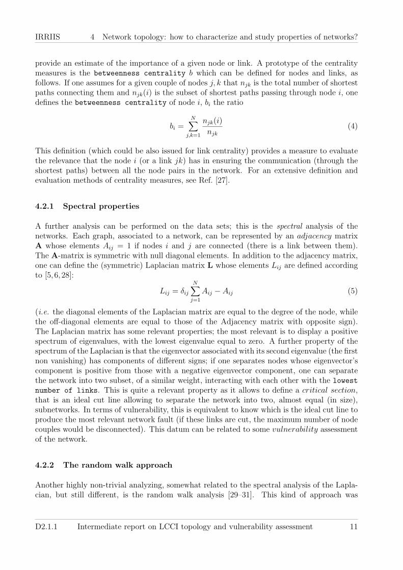
4.2.1 Spectral properties

A further analysis can be performed on the data sets; this is the spectral analysis of thenetworks. Each graph, associated to a network, can be represented by an adjacency matrixA whose elements Aij = 1 if nodes i and j are connected (there is a link between them).The A-matrix is symmetric with null diagonal elements. In addition to the adjacency matrix,one can define the (symmetric) Laplacian matrix L whose elements Lij are defined accordingto [5, 6, 28]:

Lij = δij

N∑j=1

Aij − Aij (5)

(i.e. the diagonal elements of the Laplacian matrix are equal to the degree of the node, whilethe off-diagonal elements are equal to those of the Adjacency matrix with opposite sign).The Laplacian matrix has some relevant properties; the most relevant is to display a positivespectrum of eigenvalues, with the lowest eigenvalue equal to zero. A further property of thespectrum of the Laplacian is that the eigenvector associated with its second eigenvalue (the firstnon vanishing) has components of different signs; if one separates nodes whose eigenvector’scomponent is positive from those with a negative eigenvector component, one can separatethe network into two subset, of a similar weight, interacting with each other with the lowest

number of links. This is quite a relevant property as it allows to define a critical section,that is an ideal cut line allowing to separate the network into two, almost equal (in size),subnetworks. In terms of vulnerability, this is equivalent to know which is the ideal cut line toproduce the most relevant network fault (if these links are cut, the maximum number of nodecouples would be disconnected). This datum can be related to some vulnerability assessmentof the network.

4.2.2 The random walk approach

Another highly non-trivial analyzing, somewhat related to the spectral analysis of the Lapla-cian, but still different, is the random walk analysis [29–31]. This kind of approach was



originally designed in order to reveal the large scale structure of large complex network struc-tures, like community structures [7,32–34], but has shown to be useful also for other purposes.The main idea is to introduce an auxiliary dynamic process of random walkers on the networkthat one wants to analyze. These walkers diffuse randomly around on the graph, and theywill finally reach a state of equilibrium (for undirected networks) where the density of walkersper node, or equivalently, walker current on links, reach time-independent values. What is ofinterest is on what time scale this well-defined equilibrium is reached. Mathematically thisprocess can be described by the “diffusion-like” equation:

∂tρ(t + 1) = Dρ(t) (6)

where ρ(t) is the density vector of walkers at time t, and D what can be called the diffusionmatrix (operator) for the system. This matrix is related to the adjacency matrix Aij in thefollowing way

Dij =Aij

kj

− δij, (7)

where kj refers to the connectivity of node j, and δij is the Kronecker delta function. Noticethat D is non-symmetric, unlike the adjacency and Laplacian matrices. The solution to Eq. (6)

should be readily obtained as the linear combination of v(α)exp(−λ(α)t

)where v(α) and λ(α)

are corresponding pairs of eigenvectors and eigenvalues, respectively, of the diffusion matrix.The index α is used to label the ordered sequence of eigenvalues so that α = 1 corresponds tothe largest one (that can be shown to be exactly one), α = 2 to the next-to-largest and so on.Hence one realizes that the terms corresponding to increasing α’s (where λ(α) > 0 correspondsto faster-and-faster decaying modes for the system). The interpretation of this observation isthat the largest α’s different from one (the stationary state), the slowly decaying modes, canbe related to the large scale topological features of the network. This has been demonstratedin recent publications [29–31] by plotting e.g. the current of walkers, c

(α)i = ρ

(α)i /ki, leaving

node i for an increasing number of modes α. For a given (small) mode α, the signs of the

corresponding currents, c(α)i , indicate a partitioning (into two parts) that may, or may not,

correspond to a well-defined module or cluster for the network. To determine if a givenpartitioning can be characterized as a cluster we have used the so-called modularity. It isdefined for a weighted network (of weighted adjacency matrix Wij) as [6, 35, 36]

Q =1

W∑ij

(Wij −

wiwj

W

)δκiκj

, (8)

where W =∑

ij Wij is the total “directed” weight of the graph,1 wi =∑

j Wji the weight ofoutgoing edges from vertex i, and κi denotes the community to which vertex i is assigned.If the modularity for a given partitioning is large, one says that the partitioning is a “good”module, otherwise not. By repeating this process for higher and higher (diffusive) modes, αa rather rich community structure can be identified (cf. Ref. [31] and Sec. 10 for additionaldetails).

This type of analysis may in addition give valuable information about nodes/links centralfor the stability of a network. Such nodes/links will typically be associated with the inter-connections between more-or-less well-defined modules (partitions). Furthermore, nodes/links

1For an undirected, unweighted network W is equal to two times the number of edges.


IRRIIS 5 Network reliability

corresponding to the “outer periphery” of the current mapping space are of less importancewhen dealing with stability issues. Below, one will give examples to illustrate this statement.

5 Network reliability

The present section deals with the study and development of specific algorithms for relia-bility analysis of networks, described in a form of graphs. Networks are characterized by aset of nodes (vertices) connected by directed or undirected arcs (edges). Telco, ElectricalPower Grids and Internet, all in the scope of IRRIIS, are networks that can be represented asgraphs, since the basic elements, which compose the network, can be seen as the vertices (i.e.computers or mobile nodes) of the graphs and the links (wired or wireless) the edges.

Traditional graph techniques are used to look at networks of tens or hundreds of vertices [37,38]. These techniques are based on exhaustive search algorithms intended to provide qualita-tive and quantitative information on the network connectivity, dependability, and vulnerabil-ity. In particular, the exhaustive algorithms are based on the search for all the minimal paths(minpath) connecting any pair of nodes and for all the minimal cuts (mincut) disconnectingany pair on nodes. The knowledge of all the minpaths and mincuts can be utilized to quanti-tatively evaluate the probability of connection of two nodes (reliability) or the probability ofdisconnection of two nodes (unreliability).

The present section discusses various algorithms and quantitative techniques for the exhaus-tive analysis of networks. However, the complexity of networks which are in the focus ofIRRIIS (the internet, the electrical power grids, the public telecommunication networks), canreach millions of vertices. This change of scale forces a corresponding change in the analyticapproach. Many of the approaches that have been applied in small scale networks, and manyof the questions that have been answered are simply not feasible in much larger networks.Recent years have witnessed a substantial new movement in network research [5, 8], with thefocus shifting away from the analysis of small graphs to consideration of large-scale statisticalproperties of graphs and with the aim of predicting what the behaviour of complex networkedsystems will be on the basis of measured structural properties and the local rules govern-ing individual vertices. The shift, experienced in the past few years in the understanding ofcomplex networks, was rather swift and unexpected. Empirical studies, models and analyticapproaches have revealed that real networks display generic organizing principles shared byrather different systems. These advances have created a prolific branch of statistical mechan-ics, followed with equal interest by sociologists, biologists and computer scientists. Moreover,the structural organization of a complex network influences how the system dependability andhow the system reacts to occasional failures and robust to intentional attacks.

Initially our effort, inside IRRIIS project, will be devoted to small scale networks (from tensto hundreds of nodes) for which exhaustive analysis algorithms can be implemented. Theanalytical techniques and algorithms will be described. Then we will explore the limits andthe applicability of such techniques on large scale networks.



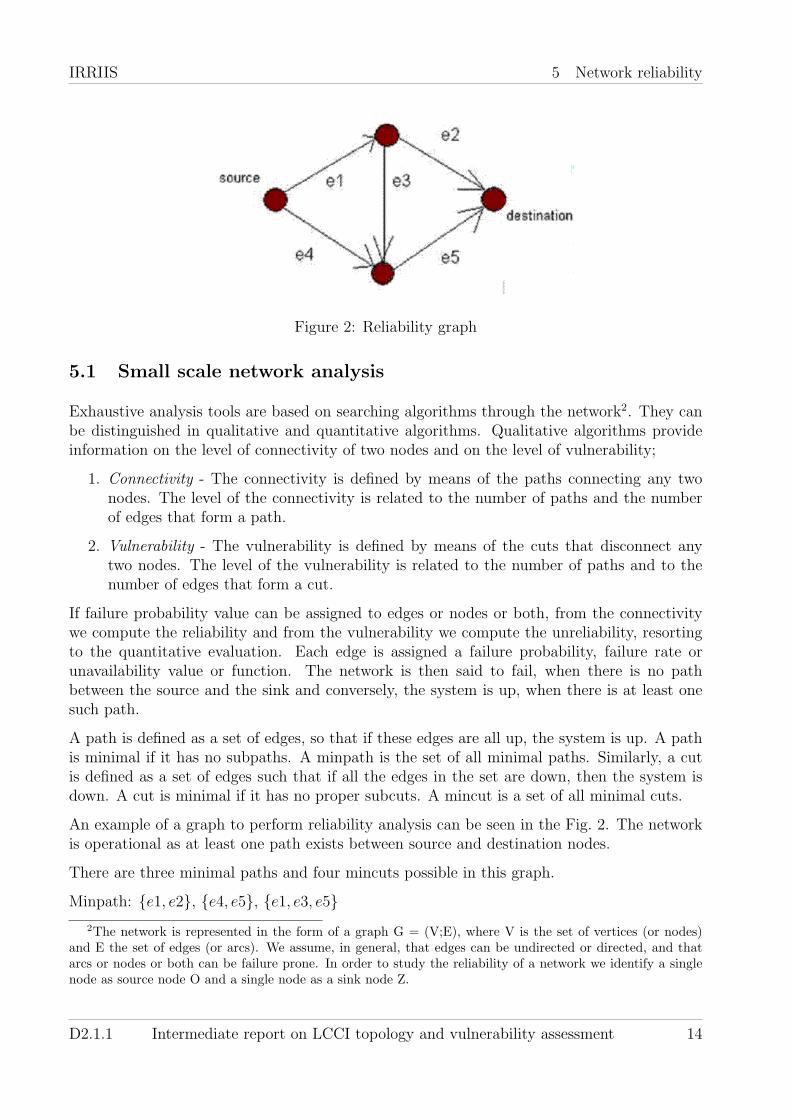
Figure 2: Reliability graph

5.1 Small scale network analysis

Exhaustive analysis tools are based on searching algorithms through the network2. They canbe distinguished in qualitative and quantitative algorithms. Qualitative algorithms provideinformation on the level of connectivity of two nodes and on the level of vulnerability;

1. Connectivity - The connectivity is defined by means of the paths connecting any twonodes. The level of the connectivity is related to the number of paths and the numberof edges that form a path.

2. Vulnerability - The vulnerability is defined by means of the cuts that disconnect anytwo nodes. The level of the vulnerability is related to the number of paths and to thenumber of edges that form a cut.

If failure probability value can be assigned to edges or nodes or both, from the connectivitywe compute the reliability and from the vulnerability we compute the unreliability, resortingto the quantitative evaluation. Each edge is assigned a failure probability, failure rate orunavailability value or function. The network is then said to fail, when there is no pathbetween the source and the sink and conversely, the system is up, when there is at least onesuch path.

A path is defined as a set of edges, so that if these edges are all up, the system is up. A pathis minimal if it has no subpaths. A minpath is the set of all minimal paths. Similarly, a cutis defined as a set of edges such that if all the edges in the set are down, then the system isdown. A cut is minimal if it has no proper subcuts. A mincut is a set of all minimal cuts.

An example of a graph to perform reliability analysis can be seen in the Fig. 2. The networkis operational as at least one path exists between source and destination nodes.

There are three minimal paths and four mincuts possible in this graph.

Minpath: {e1, e2}, {e4, e5}, {e1, e3, e5}2The network is represented in the form of a graph G = (V;E), where V is the set of vertices (or nodes)

and E the set of edges (or arcs). We assume, in general, that edges can be undirected or directed, and thatarcs or nodes or both can be failure prone. In order to study the reliability of a network we identify a singlenode as source node O and a single node as a sink node Z.



Mincut: {e1, e4}, {e1, e5}, {e2, e5}, {e2, e3, e4}

5.2 Qualitative and quantitative algorithms

Reliability analysis may be either qualitative or quantitative:

• Qualitative analysis in which connectivity or vulnerability properties between sourcenode O and sink node Z are identified. Qualitative analysis will be based on the exhaus-tive search for the minpath (connectivity) and mincuts (vulnerability).

• Quantitative analysis in which, given the probability of failure of the nodes, or arcs orboth the probability of a live connection between source node O and sink node Z (reli-ability) is computed, or alternatively, the probability of a disconnection (unreliability)between source node O and sink node Z.

It is argued that conventionally two classes of methods are used. One is the factoring algorithm,in which first an edge is chosen. Then the reliability graph is split into two graphs for eachof the cases when the chosen edge is present or absent. Then, another edge is chosen and theprocess is repeated so that finally they can be analyzed using series parallel formulas. Thusfor a graph with n edges, such a method will result in 2n cases.

The alternative conventional method is by first directly obtaining the minpaths and mincutsof the reliability graph. Then the inclusion exclusion method or the sum of disjoint productsmethod is applied to calculate the reliability. However such a method involves large numbersof minpaths and mincuts for large number of edges. This becomes too large to be stored orprocessed.

Another complimentary method is based on Binary Decision Diagrams. Binary DecisionDiagrams (BDD) have been used to represent and manipulate Boolean expressions quicklyand explicitly. They have been already used in hardware design and verification as well asreliability analysis for fault trees.

Our effort inside IRRIIS will be carried out resorting to three alternative techniques:

1. by representing the connectivity as the logical OR of the minpaths and using standardformulas for the computation of the reliability by combining the probabilities of inde-pendent events;

2. by representing the vulnerability as the logical OR of the mincuts and using standardformulas for the computation of the unreliability by combining the probabilities of inde-pendent events;

3. by representing the network connectivity by means of Binary Decision Diagrams [6], andthen computing the probabilities by searching through the BDD.

We use an algorithm which generates the BDD representing the reliability of the system as ittraverses its reliability graph. To generate a BDD, an ordering strategy is developed and theBDD is then generated with respect to that ordering strategy.


IRRIIS 6 Minpath and mincut search

6 Minpath and mincut search

The search for all the minpaths between a source node and a sink node could be implementedresorting to the Dijkstra algorithm [39], modified for the recovery of all the minimal paths ina graph. Indeed, the Dijkstra algorithm finds the minimal path, between two nodes and everyarc has associated a weight. In our case, all the arcs have weight 1 but the search must findall the minpaths.

It is expected that the algorithm for the minpath search will have the same complexity in timeas the Dijkstra algorithm, but a greater space complexity. In fact, at any step, we expect tomemorize the found paths that can be minimal and those that are incomplete.

There are various techniques and algorithms to find the mincuts of a network; we will considertwo of them:

• The first ones are based on the property that every mincut contains at least one elementof every minpath [40]) and computes all the mincuts by an exhaustive combination ofthe elements of the minpaths. Such an algorithm requires a preliminary evaluation ofall the minpaths (using, for instance the Dijkstra algorithm), and has an exponentialcomplexity because it calculates all the combinations of the minpaths elements.

• The second ones search directly the mincuts on the graph of the network [41].

6.1 Binary Decision Diagrams

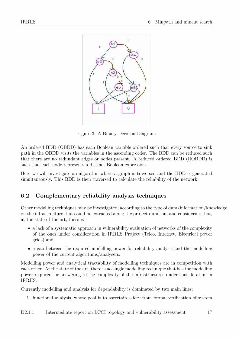
Binary Decision Diagrams are directed acyclic graphs based on Shannon’s decomposition. Thegraph has two sink nodes labelled 0 and 1 representing the two constant Boolean expressions.Each non sink note is labelled by the Boolean variable it represents and has two outgoingedges called the 0 edge (else edge) or the 1 edge (then edge) (Fig. 6.1).

To understand the representation of BDD let us look first look into Shannon’s Decomposition.

Shannon’s decomposition and the ite format

Theorem1: Let f be a Boolean expression on {x}, and x1 be a variable of {x}, then,

f = x1 · fx1=1 + x1ˆ· fx1=0,

where f evaluated in x = v is denoted by fx=v.

It can also be represented in the If-Then-Else (ite) format as

f = ite(x, F1, F2) = x1 · F1 + x1ˆ· F2,

where F1 = fx1=1 and F2 = fx1 = 0.

So looking down from the node, say of Boolean variable x. Going down the 1 edge representsthe expression when x=1 while going down the 0 edge represents the expression when x=0. Soeach node actually represents an If-Then-Else condition on the Boolean variable representedby that node.


IRRIIS 6 Minpath and mincut search

Figure 3: A Binary Decision Diagram.

An ordered BDD (OBDD) has each Boolean variable ordered such that every source to sinkpath in the OBDD visits the variables in the ascending order. The BDD can be reduced suchthat there are no redundant edges or nodes present. A reduced ordered BDD (ROBDD) issuch that each node represents a distinct Boolean expression.

Here we will investigate an algorithm where a graph is traversed and the BDD is generatedsimultaneously. This BDD is then traversed to calculate the reliability of the network.

6.2 Complementary reliability analysis techniques

Other modelling techniques may be investigated, according to the type of data/information/knowledgeon the infrastructure that could be extracted along the project duration, and considering that,at the state of the art, there is

• a lack of a systematic approach in vulnerability evaluation of networks of the complexityof the ones under consideration in IRRIIS Project (Telco, Internet, Electrical powergrids) and

• a gap between the required modelling power for reliability analysis and the modellingpower of the current algorithms/analysers.

Modelling power and analytical tractability of modelling techniques are in competition witheach other. At the state of the art, there is no single modelling technique that has the modellingpower required for answering to the complexity of the infrastructures under consideration inIRRIIS.

Currently modelling and analysis for dependability is dominated by two main lines:

1. functional analysis, whose goal is to ascertain safety from formal verification of system


IRRIIS 7 Models of common mode/cause failures

properties. Functional analysis allows the description of the evaluation arguments interms of continuous/discrete (hybrid) automata:

• hybrid models contain discrete as well as continuous variables in the same model;

• typical examples are discrete controllers that control continuous variables;

• obtainable measures are reachability properties and computer aided verification viamodel checking;

• recent techniques Hybrid Automata and Fluid Petri Nets;

2. stochastic analysis, whose aim is to provide reliability and dependability measures. Thepossibility of using a sequence of models of increasing semantically complexity to modelstochastic events of the system could be explored:

• from combinatorial models: assume statistically independent events/components(tools under consideration: Fault Tree);

• to models with localised dependencies (tools under consideration: e.g. BayesianNetworks);

• to models based on the state space: specification of all possible states of the system(for n binary events: 2n system states)

• (Tools under consideration e.g. Stochastic Petri Nets and extensions).

Along the project a significant effort will be performed for the identification of the appropriatealgorithms/tool/combination of tools to build suitable models of the infrastructures underconsideration in IRRIIS.

7 Models of common mode/cause failures

Failures of complex infrastructures (CIs) may have dramatic consequences, both organizationaland economic. The first issue that probably comes to mind in this respect is power blackouts.In Fig. 4 we depict the distribution of reported blackouts from the North American powertransmission system as an example. It is observed that the large blackouts are much lessfrequent than the smaller ones (as one probably would have expected). However, risk of anevent is normally measured by the product of its cost times its probability of occurring. Infact, it turns out that the infrequent large blackouts are more risky than the small frequentones. So in this perspective it is worth focusing on the large events.

The causes of serious CI incidents have been well documented, e.g. Knight and Amman [43]give concise summaries and pointers to the extensive reports produced by respective investi-gations. In these documented cases, adverse events occurred resulting in system failure. CIsshould be able to deal with these events in isolation as well as any coincident combination ofthese. Whether the events are likely to occur coincidentally or not depends on the nature ofthe event and, very important, on whether there are “root” events, in some cases unknown inadvance, which may cause failure in multiple, system components. Had such a common causeevent not existed then the events might have occurred independently and the likelihood of



100

101

102

103

104

Power lost in units of MW (P)

10-3

10-2

10-1

100

1-C

DF

(P)

Data (1984-2002)Data (1984-1998)

y = const. · x-1

Figure 4: The complimentary cumulative distribution (1−CDF(P)) of power lost (P) due toblackouts for the North-American electric power transmission system. (After Ref. [42])

their occurring coincidentally might have been very low. Finding out if common-cause eventsexist is important because the defenses may differ significantly depending on whether theyare truly independent or caused by a likely common cause. In the former case the combinedimpact of these events on the system may be ignored (as unlikely to occur). In the lattercase, however, adequate mechanisms of dealing with the set of common-caused events must bedevised, which may require significantly higher sophistication of the defense mechanisms thanif the events are dealt with in isolation. Even if there is no “physical”, common cause to si-multaneously trigger a set of adverse events, there might be “reasons”, e.g. hidden intellectualdifficulty, which would make it likely that the same design fault might exist in componentsacross large parts of the CIs. Thus, whenever an event triggers a design fault in one part of aCI it could also trigger it in other parts of the CI, in which the same design fault is present.

In the case of interdependent CIs, e.g. power grid and telecommunications, the CIs are part ofeach other’s environment. Thus, models of common cause/mode failure, in which the adverseeffect of the environment on the technical artefacts/systems is taken into account, are directlyapplicable to analyzing interdependencies between CIs. Simplistically put the power grid ispart of the environment in which the telecommunications system is operating and vice versa— the adequate service from the telecommunications system is part of the environment, inwhich the power grid is operating.

Over the years similar considerations to the ones outlined above for LCCIs have been studiedfor safety-critical systems. This has led to the development of various models that haveprovided useful insight into the effects of diversity on system reliability. Indeed, it is naturalto expect that similar modelling approaches will provide useful insight into resilience issuessurrounding CIs. Some relevant, notable models are

• Hughes Model,

• β-factor approach and



• Conceptual models of reliability in fault-tolerant software.

These models are briefly explained below.

7.1 Hughes model

Failure in an LCCI could be due to “unusual” environmental conditions. For instance, a nat-ural disaster such as flooding can affect the reliability of the power supply CI. A conceptuallysimilar scenario is described in the neat model due to Roger Hughes [43] in which the authoranalyses the effect of variation of the operational environment on the reliability of hardwarecomponents.3 The key conclusion from the Hughes model is that hardware components, whichmight fail independently for a given stable environment (e.g. normal conditions) are going tofail dependently, in his case of identical devices necessarily more frequently than under thenaıve assumption of failures being independent. More recently, Littlewood generalized theHughes model for the case of using diverse components, e.g. pumps from different manu-facturers [43]. The environment may affect the failure behaviour of the diverse componentsdifferently. As a result it is possible to obtain a significantly better reliability from a pairof diverse components than what is attainable with mere redundancy. Consider componentssuch that when a particular state of the environment is harmful for one of the components (i.e.leads to an increase of its conditional probability of failure) it is at the same time favorablefor the other component (its probability of failure drops down). In this case the diverse pairmay be more reliable than the non-diverse one.

7.2 β-factor approach

β-factor methodology is widely used in the safety critical industries when assessing the prob-ability of system failure of a “multi-channel systems”. The gist of the methodology is toallow for estimating the probability of common cause failure using the probability of randomhardware failure. Using β-factor methodology is an explicit recognition of the fact that as-suming independence of channel failures is unreasonable. The β-factor methodology is also anattempt to provide a feasible engineering solution for calculating the system unreliability, e.g.Ref. [43]. In practice, the use β-factor, e.g. Ref. [43], entails applying a scoring procedure tothe system being evaluated, according to some dependability-relevant criteria.4

Somewhat related to β-factor approach are other engineering approaches to assessing theimpact of common cause failures. Some guidelines, such as “Safety Assessment Principlesfor nuclear facilities”5, go on further to specify a “cut-off” value for the probability of failureachievable using identical, redundant components. A cut-off value of up to 10−5 represents ajudgement by NII6 of the best limit, which could reasonably be supported for a simple system

3In his context Hughes refers to components used in electrical power production plants such as water pumps.4Criteria such as diversity/redundancy, complexity/design/application/maturity/experience, assess-

ment/analysis and feedback of data, competence/training/safety culture and environmental control.5This is a recent document published for comment by the Crown Health and Safety Executive, Ref. [43],

p.31, explicitly discusses the use of redundancy, diversity and segregation ’? within the design of structuressystems and components important to safety so as to achieve the required level of reliability?’.

6Nuclear Installations Inspectorate.


IRRIIS 8 Critical infrastructures

by currently available data and methods of analysis [43]. Values smaller than 10−5 can only beaccepted in exceptional circumstances; when the “duty holders” present the regulators with astrong case to support the claim. The value 10−5, however, should not be used automatically.Depending on the complexity of the system larger cut-off values can be used (10−4 and even10−3 are explicitly mentioned in Ref. [43]. Using cut-off values is a mechanism complementaryto β-factors, trying to alleviate the difficulties in assessing the probabilities of failures in caseswhen common cause failures are a concern.

7.3 Conceptual models of reliability of fault-tolerant software

Conceptual probabilistic models of fault-tolerant software have been developed in the secondhalf of the 1980s and provide a convincing explanation of the limitations of design diversity:essentially they explain that via design diversity one should only expect modest improvementof software reliability. The first major breakthrough in stochastic modelling of diversity camein a paper by Eckhardt and Lee [43]. The key idea here was that the different demandsthat a program might receive during operation would vary in “difficulty” — specifically theprobability of failure upon execution of a demand would be different for different demands.7

From this insight it is possible to show that if more than one version executes each demand,the failures of the versions cannot be independent: in fact they will exhibit dependence infailure behaviour which ensures that fault tolerant systems built from the versions will be lessreliable, on average, than if independence could be assumed.

The model was later generalized [43] to take account of forced diversity (LM model), where thedifferent teams would be required by a higher design authority to use different methodologies:for example different programming languages, testing and analysis techniques, etc. Here theintent was to exploit the possibility that what might be “difficult” for one methodology maybe easy for another. In this model, it can be shown that it is no longer inevitable that a faulttolerant system will be less reliable than would be the case if the versions failed independently.Some empirical studies, e.g. Ref. [43], have confirmed that negative correlation can indeedoccur in practice.

8 Critical infrastructures

It should now be rather clear that the topic of this report is Critical Infrastructures. But whatmakes an infrastructure critical? Within IRRIIS one has adopted the following definition8: Acritical infrastructure is a large scale infrastructure which if degraded, disrupted or destroyed,would have a serious impact on health, safety, security or well-being of citizens or the effectivefunctioning of governments and/or economy.

Accordingly to this definition the following infrastructures may be labeled as critical:

7In the original papers by Knight and Amman [43] the term “input” was used instead of “demand”. Herewe refer to demand to avoid the confusion surrounding the term ’input’ used in different contexts. A demandcan consist of a single or many inputs to the software depending on the system context.

8This definition was originally formulated by Walter Schmitz.



• Public power supply network

• The Telecommunication network

• The Internet

Below we will briefly describe these networks, and say something about what is characteristicfor them.

8.1 Public power supply networks

The public power supply network transmits power from generation to loads thereby providingthe link between producers and consumers. The network connects large numbers of gener-ators and loads together thus i)improving the reliability of the power supply, ii) reducingneeds for reserve, peak, control and storage capacity, iii) enabling more efficient and economicpower production, and iv) providing a necessary platform for the electricity market. Thestrengthening of the cross border transmission capacity has made the public power supplynetwork increasingly international and spatially very extended. The power supply network isan essential, but often very international part of the national critical infrastructure.

The power supply network is hierarchically organized to transmission and distribution net-works. Transmission networks cover very wide geographical areas, and has typically very highvoltage levels and big power flows. It is operated as a meshed network. Distribution net-works, on the other hand, connect the loads and distributed generation with the transmissionnetwork. The distances are traditionally shorter and the voltage level lower than in the trans-mission network. The distribution networks are normally organized in a radial way althoughredundancy is provided by a meshed network topology. Low voltage customers are connectedto the distribution network via low voltage distribution networks.

About one third of the cost of power supply comes from the distribution of power. The powerdistribution network has also a much higher impact on the reliability and power quality thanthe power transmission network. The transmission network failures are relatively rare, buttheir impact can influence much wider areas than distribution failure impacts.

Power network is characterized by the fact that it has very little buffering storage capacityand the physical balance of supply and demand must be maintained or the power transmissionsystem will collapse. The deregulated electricity market is an important tool for finding acost efficient initial solution for this balancing problem. Operation of the power network ishighly and increasingly dependent on protection, automation, information and communicationsystems.

Distributed generation, intermittent generation from renewable energy sources (e.g. windenergy), pressures to cost reductions and power quality improvements, ever bigger generationand transmission units are expected challenges to the power network. These call for significantchanges in the power distribution systems and their automation and operation, but the powerdistribution systems have much inertia. The required lifetime of the power network relatedinvestments is very long. Thus rapid fundamental changes are seldomly possible.



From the topological point of view, the graphs representing electrical transmission networkscannot be properly ascribed to random nor to SF networks. In fact, as it happens fornetworks whose structure is constrained (i.e. by geographical reasons) or who cannot presentan arbitrarily large node’s degree (as it happens for roads, for instance, where there is avery low maximum degree), electrical networks have an exponential distribution of node’sdegree [44,45].

8.2 The telecommunication networks

The PSTN (Public Switched Telephone Network) is mainly defined by ITU-T standards. Itconsists of an almost entirely digital network, only the last mile being still analog. In recentyears, digital services have been increasingly rolled out to end users using services such as DSLover the analog line. A typical telephone call represents 64 kbit/s (1 byte every 125 micro-seconds). As far as a connection is concerned in the classical PSTN, it may involve merelyvoice-frequency transmission through a single end office or it may involve a multiplicity oflinks including several offices, voice-frequency paths and carrier systems. The telephone setconverts acoustic energy into an electrical analog signal and also converts the received signalto its acoustic form. In addition, it generates supervisory signals (like on-hook and off-hook)and the address information used by the switching system to establish connections. Thecustomer loop provides a path for the two way speech signals and the ringing, switching, andthe supervisory signals. The small percentage of the time that the customer loop is actuallyused has led to the consideration of line concentrators for introduction between the customerand the central office. This concentrator allows many customers to share a limited numberof lines to the central office. The audio sound is digitized at an 8 kHz sample rate using8-bit pulse code modulation. The call is then transmitted in the digital network. The linefrom the concentrator to the central office is a trunk, whose main difference with a loop isthat a loop is permanently associated with a customer whereas a trunk is a common usageconnection. Trunks of various types are used to connect end offices and toll centers. A directinteroffice trunk connects one end office to another end office; a tandem trunk connects anend office to an intermediate or tandem office; and a toll connecting trunk connects an endoffice to a toll office. Up to the point where the signals are connected to intertoll trunksin the toll office, the message and supervisory signals may be handled on a two-wire basis(the same pair of wires is used for both directions of transmission), or on a four-wire basis(separate transmission paths for each direction). At the toll office after appropriate switchingand routing, the signals are generally connected to intertoll trunks by means of a four-wireterminating set, which splits apart the two directions of transmission so that the long-haultransmission may be accomplished on a four-wire basis. Through these intertoll trunks, thesignals are transmitted to remote toll-switching centers (which in turn may be connectedby intertoll trunks to other switching centers) and ultimately reach the recipient of the callthrough a toll-connecting trunk an end office, another four-wire terminating set and localswitching equipment, and a final customer loop. There are five ranks or classes of switchingcenters (the regional center, the sectional center, the primary center, the toll center, and theend office which is the telephone exchange where the customer loop terminates). This offersseveral possible routes from a source to a destination, based on the chain of switching thatis selected. The access network and inter-exchange transport of the PSTN use synchronous


IRRIIS 9 Collected data sets

optical transmission (SONET and SDH) technology, although some parts still use the olderPDH technology.

8.3 The Internet

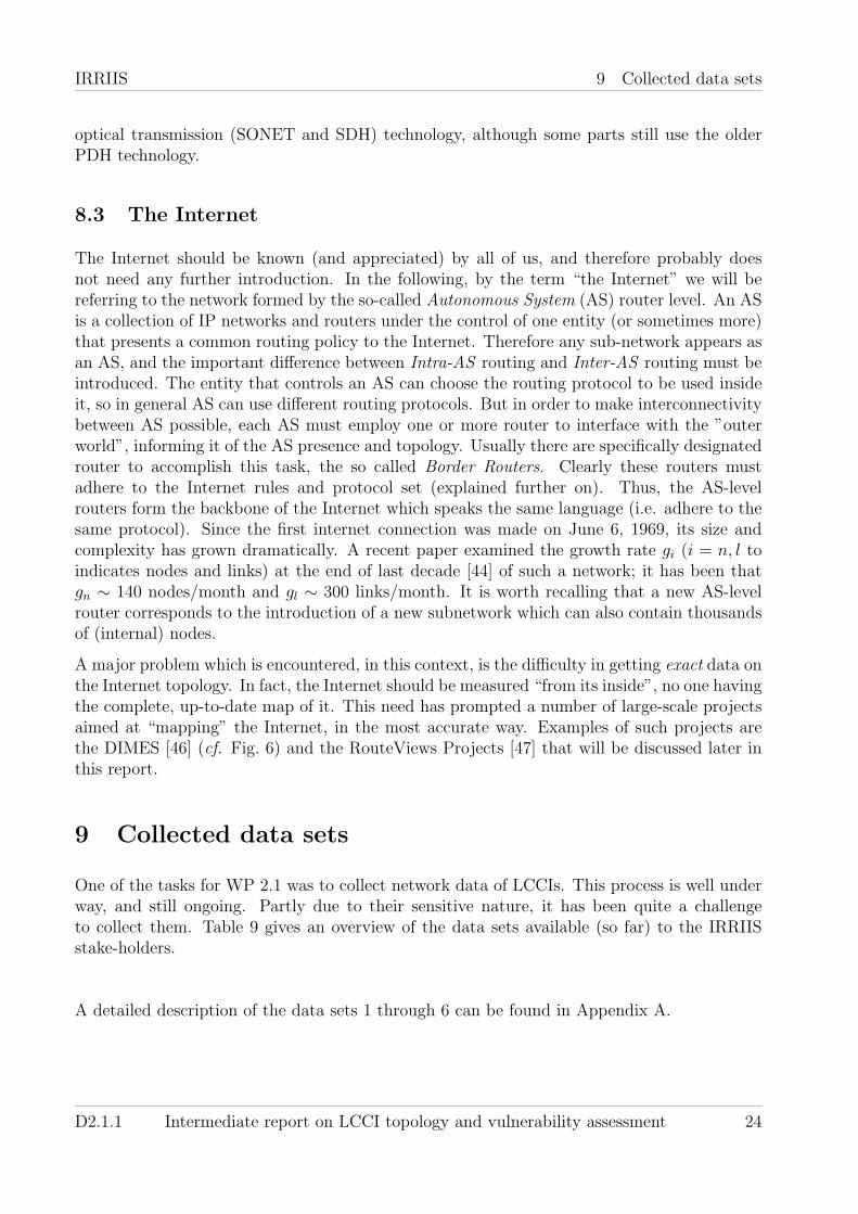
The Internet should be known (and appreciated) by all of us, and therefore probably doesnot need any further introduction. In the following, by the term “the Internet” we will bereferring to the network formed by the so-called Autonomous System (AS) router level. An ASis a collection of IP networks and routers under the control of one entity (or sometimes more)that presents a common routing policy to the Internet. Therefore any sub-network appears asan AS, and the important difference between Intra-AS routing and Inter-AS routing must beintroduced. The entity that controls an AS can choose the routing protocol to be used insideit, so in general AS can use different routing protocols. But in order to make interconnectivitybetween AS possible, each AS must employ one or more router to interface with the ”outerworld”, informing it of the AS presence and topology. Usually there are specifically designatedrouter to accomplish this task, the so called Border Routers. Clearly these routers mustadhere to the Internet rules and protocol set (explained further on). Thus, the AS-levelrouters form the backbone of the Internet which speaks the same language (i.e. adhere to thesame protocol). Since the first internet connection was made on June 6, 1969, its size andcomplexity has grown dramatically. A recent paper examined the growth rate gi (i = n, l toindicates nodes and links) at the end of last decade [44] of such a network; it has been thatgn ∼ 140 nodes/month and gl ∼ 300 links/month. It is worth recalling that a new AS-levelrouter corresponds to the introduction of a new subnetwork which can also contain thousandsof (internal) nodes.

A major problem which is encountered, in this context, is the difficulty in getting exact data onthe Internet topology. In fact, the Internet should be measured “from its inside”, no one havingthe complete, up-to-date map of it. This need has prompted a number of large-scale projectsaimed at “mapping” the Internet, in the most accurate way. Examples of such projects arethe DIMES [46] (cf. Fig. 6) and the RouteViews Projects [47] that will be discussed later inthis report.

9 Collected data sets

One of the tasks for WP 2.1 was to collect network data of LCCIs. This process is well underway, and still ongoing. Partly due to their sensitive nature, it has been quite a challengeto collect them. Table 9 gives an overview of the data sets available (so far) to the IRRIISstake-holders.

A detailed description of the data sets 1 through 6 can be found in Appendix A.


IRRIIS 10 The LCCI network analysis

Set No. Short Description No. of nodes Format Delivered by1 Power Grid: European High and

Highest Voltage∼ 300 PS (partly ASCII) Glueckauf-Verlag

2 Power Grid: National High Volt-age

100–10000 PDF/ASCII World Wide Web

3 Power Grid: Regional Distribu-tion Networks

∼ 100 MS-Access Siemens

4 Internet: AS-router level > 10000 ASCII ENEA5 TelCo-Networks: principal

sketch of national networkText Telecom Italia

6 Miscellaneous

Table 1: On overview of the LCCI network data sets that are available within IRRIIS.

10 The LCCI network analysis

In this section, we will present the present results for the topological analysis that has beenperformed on the collected LCCI networks that were described in the previous section (Sec. 9).The description of the methods used have already been presented in Sec. 4 and referencestherein.

(a) The Italian transmission grid (b) The min-cut of the Italian grid

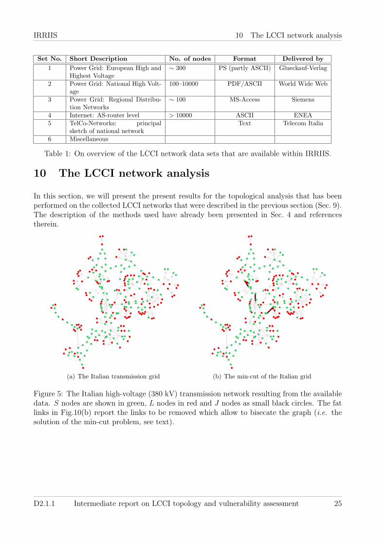
Figure 5: The Italian high-voltage (380 kV) transmission network resulting from the availabledata. S nodes are shown in green, L nodes in red and J nodes as small black circles. The fatlinks in Fig.10(b) report the links to be removed which allow to bisecate the graph (i.e. thesolution of the min-cut problem, see text).



Figure 6: The network of AS collected by the Dimes Project [46]. The network consists ofN = 14, 154 nodes, located all over the world, and nearly L = 40, 000 links inter-connectingthem. This graph shows one example of why visualizing a large network is not fully uncoveringits topology.

10.1 Topological analysis

10.1.1 The Italian high–voltage (380 kV) electrical transmission network

We have analyzed power grid data relative to the Italian high-voltage (380 kV) transmissionline (HVIET, hereafter). Data have been deduced from the analysis of the public documen-tation (Gazzetta Ufficiale) where the network owners must constantly indicate the currentnetwork configuration (in terms of nodes and lines, length, ownerships etc.) and its updates.HVIET can be represented by an undirected graph of N nodes and E edges or links (i.e. powertransmission lines). The available data do allow to simply attribute to each node the qualityof being a source node (or generator) S (where part of the power is inserted in the network),a load node L (where part of the power is extracted from the network) and a junction node J(which is neither an S nor an L node). The topology of the HVIET is reported in Fig. 10(a)where S nodes are green, L nodes are red and J nodes are small black circles. HVIET consistsof N = 310 nodes and E = 359 links. There are S = 117 nodes, L = 139 nodes and J = 54



1 10k

1

10

100

P(k)

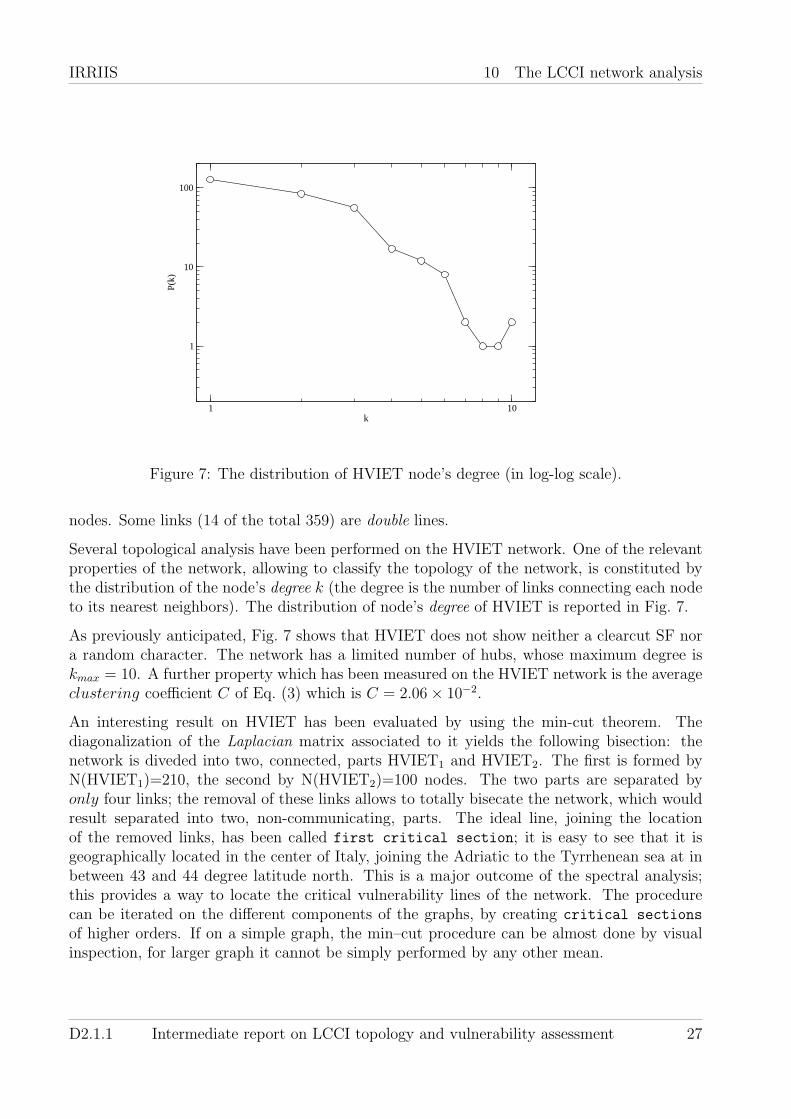
Figure 7: The distribution of HVIET node’s degree (in log-log scale).

nodes. Some links (14 of the total 359) are double lines.

Several topological analysis have been performed on the HVIET network. One of the relevantproperties of the network, allowing to classify the topology of the network, is constituted bythe distribution of the node’s degree k (the degree is the number of links connecting each nodeto its nearest neighbors). The distribution of node’s degree of HVIET is reported in Fig. 7.

As previously anticipated, Fig. 7 shows that HVIET does not show neither a clearcut SF nora random character. The network has a limited number of hubs, whose maximum degree iskmax = 10. A further property which has been measured on the HVIET network is the averageclustering coefficient C of Eq. (3) which is C = 2.06× 10−2.

An interesting result on HVIET has been evaluated by using the min-cut theorem. Thediagonalization of the Laplacian matrix associated to it yields the following bisection: thenetwork is diveded into two, connected, parts HVIET1 and HVIET2. The first is formed byN(HVIET1)=210, the second by N(HVIET2)=100 nodes. The two parts are separated byonly four links; the removal of these links allows to totally bisecate the network, which wouldresult separated into two, non-communicating, parts. The ideal line, joining the locationof the removed links, has been called first critical section; it is easy to see that it isgeographically located in the center of Italy, joining the Adriatic to the Tyrrhenean sea at inbetween 43 and 44 degree latitude north. This is a major outcome of the spectral analysis;this provides a way to locate the critical vulnerability lines of the network. The procedurecan be iterated on the different components of the graphs, by creating critical sections

of higher orders. If on a simple graph, the min–cut procedure can be almost done by visualinspection, for larger graph it cannot be simply performed by any other mean.



10.1.2 The world–wide Internet network at the autonomous system–level (AS)routers

Data have been collected from two different sources [46,47] related to two independent projects,DIMES and RouteViews, funded by EU and US, respectively. In the present document, wedo not report details on the technical methods at the basis of the search and the assembly ofthe Internet maps (for that, the reader could refer to [48, 49]). We will focus, in turn, on theanalysis of the resulting graphs (cf. Fig. 6), constructed on the basis of the available data.Data usually consist of snapshots of the map taken at a given date (in terms of couples onconnected nodes). A repository of several snapshots, collected at different times, is usuallycontained in the projects web sites. These are useful as they allow to monitor the growth of thenetwork (or, at least, its time variation); these data could be used to infer growth mechanismsunderlying the time variation of the networks properties (size, degree, clustering etc.) [44].

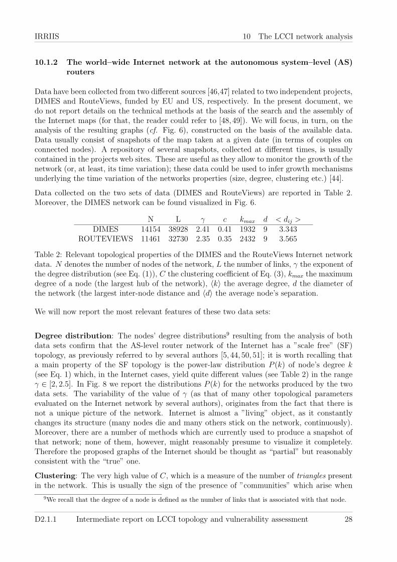
Data collected on the two sets of data (DIMES and RouteViews) are reported in Table 2.Moreover, the DIMES network can be found visualized in Fig. 6.

N L γ c kmax d < dij >DIMES 14154 38928 2.41 0.41 1932 9 3.343

ROUTEVIEWS 11461 32730 2.35 0.35 2432 9 3.565

Table 2: Relevant topological properties of the DIMES and the RouteViews Internet networkdata. N denotes the number of nodes of the network, L the number of links, γ the exponent ofthe degree distribution (see Eq. (1)), C the clustering coefficient of Eq. (3), kmax the maximumdegree of a node (the largest hub of the network), 〈k〉 the average degree, d the diameter ofthe network (the largest inter-node distance and 〈d〉 the average node’s separation.

We will now report the most relevant features of these two data sets:

Degree distribution: The nodes’ degree distributions9 resulting from the analysis of bothdata sets confirm that the AS-level router network of the Internet has a ”scale free” (SF)topology, as previously referred to by several authors [5, 44, 50, 51]; it is worth recalling thata main property of the SF topology is the power-law distribution P (k) of node’s degree k(see Eq. 1) which, in the Internet cases, yield quite different values (see Table 2) in the rangeγ ∈ [2, 2.5]. In Fig. 8 we report the distributions P (k) for the networks produced by the twodata sets. The variability of the value of γ (as that of many other topological parametersevaluated on the Internet network by several authors), originates from the fact that there isnot a unique picture of the network. Internet is almost a ”living” object, as it constantlychanges its structure (many nodes die and many others stick on the network, continuously).Moreover, there are a number of methods which are currently used to produce a snapshot ofthat network; none of them, however, might reasonably presume to visualize it completely.Therefore the proposed graphs of the Internet should be thought as “partial” but reasonablyconsistent with the “true” one.

Clustering: The very high value of C, which is a measure of the number of triangles presentin the network. This is usually the sign of the presence of ”communities” which arise when

9We recall that the degree of a node is defined as the number of links that is associated with that node.



1 10 100Node degree, k

1

10

100

1000

10000

Nod

e de

gree

occ

urra

nce,

P(k

)

RouteViews network, N = 11461DIMES network, N = 14154

Figure 8: The distribution of node degree of the networks generated by the DIMES and theRouteViews data.

neighbors of a common node become neighbors of each other. The value of C is usually verylow for random networks. Further details on how the Internet is structured can be obtainedby the analysis of the correlation between the clustering and the degree of each node.

Diameter: The network’s diameter which, as in a typical case of a ”small world” system, isquite low. The expected value of the

drand =logN

log 〈k〉(9)

which, in our cases, would have produced similar values such as drand = 9.14 for DIMES anddrand = 8.92 for RouteViews. This is a quite controversial point in the literature. Standingon their analysis, some authors have claimed an Internet diameter higher than that predictedfor a random networks [50], others have measured a slightly lower diameter [5]. For thiscontroversy, the same point raised above holds (there are many pictures of the Internet).However, the relevant issue is that the Internet, although being a scale-free network and, assuch, with an expected diameter larger than that of a random network of similar size, has, inturn, the diameter which is as low as that of a random network. This is relevant observationas the growth mechanism of the network is “clever” enough to produce such a property (whichis indeed a relevant property for a network to have). Fig. 9 reports the distribution of theinter–node distances for the DIMES and the RouteViews graphs.

Growth mechanisms: We have attempted to define an “empirical” growth mechanismsallowing to reproduce the most relevant features (the value of γ of the P (k) distribution andthe very high value of C). We succeded in this task: the resulting recipe for growing sucha network comes out from a suitable combination of the “preferential attacchment” (PA)mechanism, introduced by Barabasi [5] and its further modifications, and the so–called ”triadformation” (TF), introduced by Holme [26] and already used to define a growth mechanismfor the Internet [44]. In our case, the rule for growing the Internet is the following: if P(n+1)→j



0 2 4 6 8node distance

0

1e+07

2e+07

3e+07

4e+07

5e+07

6e+07

node

dis

tanc

e oc

curr

ance

DIMES network, N = 14154RouteViews network, N = 11461

Figure 9: The distribution of inter-node distances in the DIMES and the RouteViews graphs.

is the probability that a new node (n + 1) sticks on the node j belonging to the network,presently composed of n nodes, it will be as follows:

P(n+1)→j = (1− β)PAα + βTF (10)

It means that the new node will stick with a probability (1−β) with a modified PA algorithm(indicated as PAα) or with probability β with a TF mechanism. The modification of the PAmechanism (indicated in Eq. (10 ) as PAα) consists in the following: the node j of the existingnetwork is linked with a probability

P(n+1)→j =kα

jn∑i

ki

. (11)

In our cases the value of the parameters providing the best agreement with the DIMES dataset are: β = 0.93 and α = 1.44.

The random walk approach : We will now analyze the topology of the Internet by therandom walk current mapping technique described in Sec. 4.2.2. We here consider an AS-dataset obtained from Ref. [52]. It consists of about 6 500 nodes from various parts of the world.

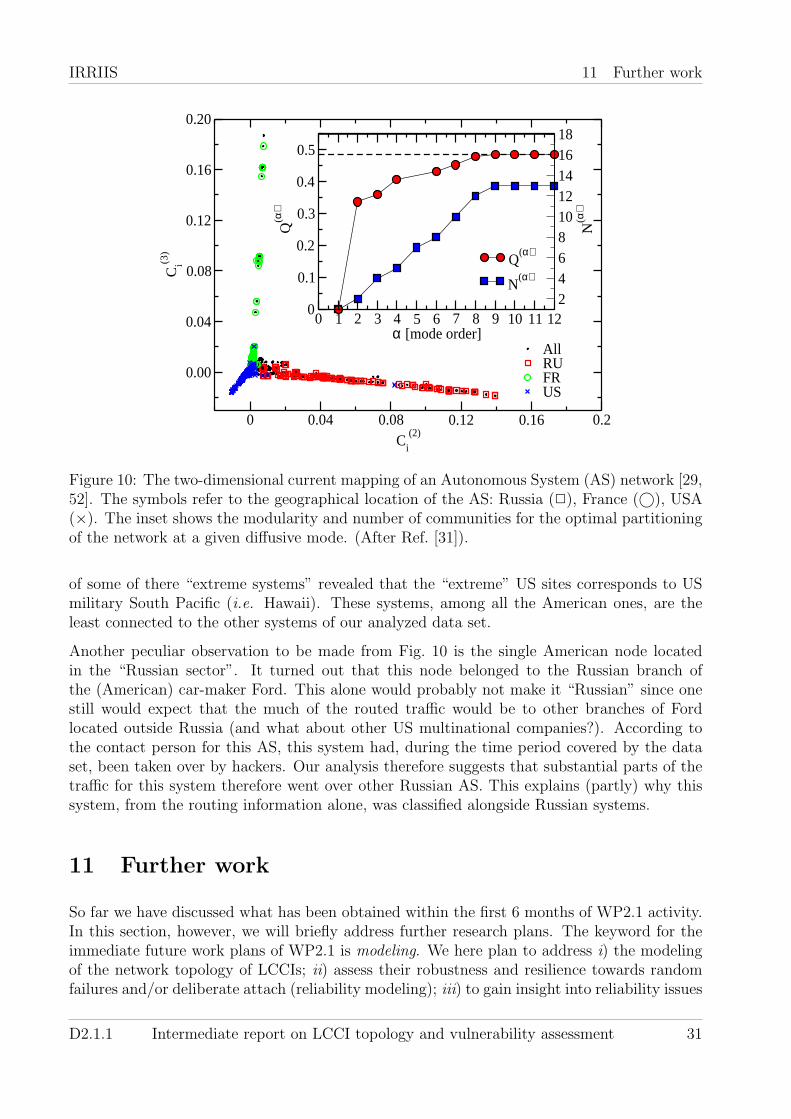
Fig. 10 shows the 2-dimensional current mapping of the networks using the two slowest de-caying diffusive modes, i.e. α = 2, 3. All system have been labelled with black dots. Laterall nodes from some selected nations have in addition been labeled differently for convenience.The star-like structure indicates that there is a hierarchy of vertices where those located thefurthest away from the origin of the current plot are the most peripheral vertices of the net-work. Furthermore, each hierarchy corresponds roughly to the national division of the ASnetwork. Fig. 10 shows that the three legs of the star-structure correspond to Russia, the USand France. For the AS-network we identified 13 communities resulting in a modularity ofabout one-half (inset to Fig. 10).

This analysis indicates that the extreme edges of the Internet corresponds to US (blue crossesin Fig. 10) and Russian (red squares) AS. A closer investigation into the location and purpose


IRRIIS 11 Further work

24681012141618

N(α

)

N(α)

0 1 2 3 4 5 6 7 8 9 10 11 12α [mode order]

0

0.1

0.2

0.3

0.4

0.5

Q(α

)Q

(α)

0 0.04 0.08 0.12 0.16 0.2C

i

(2)

0.00

0.04

0.08

0.12

0.16

0.20

Ci(3

)

AllRUFRUS

Figure 10: The two-dimensional current mapping of an Autonomous System (AS) network [29,52]. The symbols refer to the geographical location of the AS: Russia (2), France (©), USA(×). The inset shows the modularity and number of communities for the optimal partitioningof the network at a given diffusive mode. (After Ref. [31]).

of some of there “extreme systems” revealed that the “extreme” US sites corresponds to USmilitary South Pacific (i.e. Hawaii). These systems, among all the American ones, are theleast connected to the other systems of our analyzed data set.

Another peculiar observation to be made from Fig. 10 is the single American node locatedin the “Russian sector”. It turned out that this node belonged to the Russian branch ofthe (American) car-maker Ford. This alone would probably not make it “Russian” since onestill would expect that the much of the routed traffic would be to other branches of Fordlocated outside Russia (and what about other US multinational companies?). According tothe contact person for this AS, this system had, during the time period covered by the dataset, been taken over by hackers. Our analysis therefore suggests that substantial parts of thetraffic for this system therefore went over other Russian AS. This explains (partly) why thissystem, from the routing information alone, was classified alongside Russian systems.

11 Further work

So far we have discussed what has been obtained within the first 6 months of WP2.1 activity.In this section, however, we will briefly address further research plans. The keyword for theimmediate future work plans of WP2.1 is modeling. We here plan to address i) the modelingof the network topology of LCCIs; ii) assess their robustness and resilience towards randomfailures and/or deliberate attach (reliability modeling); iii) to gain insight into reliability issues


IRRIIS A Detailed data description

via modeling of cascading failures. Such works rely on the network topologies of LCCIs beingwell known, and therefore, such studies have only very recently started to be addressed withinWP2.1. In the future, more and more of the work of this Work Package will be focused ontothese tasks. One of the goals is to identify possible failure indicators.

12 Summary and conclusions

Large Complex Critical Infrastructures (LCCI) are national — or international — wide tech-nological systems whose correct functioning has an high social impact. Among them, thenetworks for the transmission and the distribution of electrical power and those allowing com-munications to occur (in all its forms, from phones to the Internet) play a central role; as mostof the LCCIs are tightly interdependent, energy and communication networks have the largestimpacts on the correct functioning of many other networks. This report is mainly addressedto the analysis of these classes of networks by using methods and models provided by theanalysis of their basic structure.

The analysis of LCCIs can be carried out at different levels. The basic level is provided bythe analysis of their topological structure which can be carried out on basic (sharable andunrestricted) structural data. In fact, LCCIs can be mapped onto complex graphs which canbe analysed by methods recently developed in Graph Theory. These analyses might provideinteresting insights on the networks’ properties, particularly on their “structural vulnerability”and be the starting point for the definition of dynamical model of the networks’ functioning tobe used for the study of more complex properties, such as, for instance, LCCI interdependency.

In this intermediate report, we have documented the current activity, focus, and achievementsobtained during the first 6 months period of the Working Package WP2.1 of the IRRIISproject. Furthermore, the direction of further research has been briefly outlined. We canconclude that the work of WP2.1 is very much on-going, and in accordance with the workplan outline in the IRRIIS proposal. Future research in addition to the ongoing activity ontopological analysis will focus on robustness and reliability studies and modeling of LCCIs.Interesting and important results are expected in the near future.

A Detailed data description

In this appendix, a more detailed overview is given of the (network) data sets that have beencollected so far within IRRIIS.

For those that have access to the BSCW server, the available data sets can be downloadedfrom https://bscw.sit.fraunhofer.de/bscw/bscw.cgi/692344. Most data sets are equipped witha short text header describing the data and from where they were obtained.


IRRIIS A Detailed data description

A.1 Power grid data

Several data sets of different size and level of detail have been collected both for the transmis-sion and the distribution level.

A.1.1 European transmission power grid overview data

This data set originally is a digital map in the pdf-format that was purchased from the GermanGlueckauf-Verlag. The map contains highest voltage power lines from 300 to 750kV, powerstations larger 500MW and transforming stations. With less then 1000 nodes it seems obviousthat the map is not comprehensive and contains a selection of the mentioned devices only.Moreover, the pdf-format makes mathematical analysis cumbrous, but feasible.

A.1.2 National high voltage transmission power grid data

For three regions in Europe we were able to find more detailed highest and high voltage maps onthe Web, also in pdf-format. These are Spain, Germany, and north western Europe includingneighboring countries. Basically, the content is the same as in data set 1, although morenodes are depicted. For Italy and the US, in addition we have been able to collect adjacencymatrices for the highest voltage grid with approximately 300 and 5000 nodes respectively. Thenetwork edges are not weighted and both sets do not contain any geographical data. For theUS data set, no additional information is given about the node type, while such informationis available for the Italian data set.

A.1.3 Selected power grid test data at distribution level

Delivered by Siemens, we acquired two test data sets designed for usage with the softwarepackages SINCAL and NETOMAC. The first set contains the power grid of a (for us unknown)20, 000 inhabitant town in central Europe containing power lines down to 400V interlinkingabout 120 nodes. The data set is available in the MS ACCESS format. The second distributionlevel data set is optimized for dynamic simulations with NETOMAC representing a 30 bus testcase called “New England” and presumably equivalent to the real network in New England(USA) in the 1960’s.

A.2 Internet adjacency data at AS-router level

From the DIMES-Project [46] an adjacency matrix of the Internet at AS-level was collected.This data set contains about 14, 000 nodes and ca. 40, 000 edges (cf. Tab. 2 The same datawas gathered using a different method by the RouteViews initiative [47]. It was lead by theUniversity of Oregon. Both data sets are comparable in size. Notice that there is also dataavailable from an older (no longer maintained) project at Ref. [52].


IRRIIS References

A.3 Telecommunication network

To collect telecommunication network data is a challenging and an ongoing process withinIRRIIS. So far no data set has been made available to IRRIIS, but discussion with IRRIISstake-holders are under way for this purpose. One expects to have available such data setsin the near future. The main challenges to be overcome have been security issues relatedto the sensitive nature of such data. Moreover, much effort was required to improve thecommunication between various partners of IRRIIS in order to make sure that “one speaks thesame language”. This is important in order to be able to gain a better understanding of whatkind of data are available, and which are the interesting ones from an IRRIIS perspective.This has been a somewhat time consuming process due to the fact that, for instance, thepower and telecommunication networks are rather different in many respects. People from thedifferent communities need time to be able to realize and grasp the consequences and maybeeven appreciate the differences between these two classes of LCCI networks. For the powernetworks the physical layer is the dominating one. For the telecommunication counterpart,however, there are many more layers and they are much more complex in the way they areorganized. For this latter network type, the logical layer often plays an as important role asthe physical.

A.4 Miscellaneous data

For dynamical simulations of power grids an exhaustive archive of test cases can be foundat [53]. Though not considered in the analysis so far, these data sets might turn out to befruitful for further investigations.

References

[1] US-Canada Power System Outage Task Force. Final report of the august 14th blackoutin us and canada. Technical report, United States Department of Energy and NationalResources Canada, April 2004.

[2] Source:. http://mit.edu/vdb/www/6.977/l-blondel.pdf.

[3] W.W. Zachary. J. Anthropol. Res., 33:452473, 1977.

[4] D.J. Watts and S.H. Strogatz. Collective dynamics of ’small-world’ networks. Nature,393(6684):440–443, 1998.

[5] R. Albert and A.-L. Barabsi. Statistical mechanics of complex networks. Rev. Mod. Phys.,74:47–97, 2002.

[6] M.E.J. Newman. The structure and function of complex networks. SIAM Review,45(2):167–256, 2003.

[7] S. Boccaletti, Y. Moreno, V. Latora, M. Chavez, and D.U. Hwang. Complex networks:Structure and dynamics. Phys. Rep., 424:175–308, 2006.


IRRIIS References

[8] S.N. Dorogovtsev and J.F.F. Mendes. Evolution of networks. Adv. Phys., 51:1079–1187,2002.

[9] R. Albert, H. Jeong, and A. L. Barabsi. Error and attack tolerance of complex networks.Nature, 406:378 – 382, 2000.

[10] Y. Moreno, J.B. Gomez, and A.F. Pacheco. Instability of scale-free networks under node-breaking avalanches. Europhys. Lett., 58:630–636, 2002.

[11] Y.C. Lai A.E. Motter. Cascade-based attacks on complex networks. Phys. Rev. E,66:065102, 2002.

[12] X.F. Wang and J. Xu. Cascading failures in coupled map lattices. Phys. Rev. E,58(1):056113, 1998.

[13] P. Crucitti, V. Latora, and M. Marchiori. Model for cascading failures in complex net-works. Phys. Rev. E, 69:045104, 2004.

[14] A.E. Motter. Cascade control and defense in complex networks. Phys. Rev. Lett.,93:098701, 2004.

[15] B.A. Carreras, V.E. Lynch, I. Dobson, and D.E. Newman. Critical points and transitionsin an electric power transmission model for cascading failure blackouts. Chaos, 12(4):985–994, 2002.

[16] R. Albert, I. Albert, and G.L. Nakarado. Structural vulnerability of the north americanpower grid. Rev. Mod. Phys., 74:47–97, 2002.

[17] T. Ohira and R. Sawatari. Phase transition in a computer network traffic model. Phys.Rev. E, 58(1):193–195, 1998.

[18] International journal of critical infrastructures. http://www.inderscience.com/browse /in-dex.php?journalID=58.

[19] W.W. Leontief. Input-Output Economies. Oxford University Press, New York, 2nd edi-tion, 1986.

[20] L. Issacharoff, S. Bologna, V. Rosato, G. Dipoppa, R. Setola, and E. Tronci. A dynamicalmodel for the study of complex systems’ interdependence. In CNIP 2006, Rome, 2006.

[21] S. Panzieri, R. Setola, and G. Ulivi. An approach to model complex interdependentinfrastructures. In 16th IFAC World Congress, Praha, 2005.

[22] P. Jiang and Y.Y. Haimes. Risk management for leontief-based interdependent systems.Risk Analysis, 24(5):1215–1229, 2004.

[23] L. Buzna, K. Peters, and D. Helbing. Modelling the dynamics of disaster spreading innetworks. Phys. A, 363:132–140, 2006.

[24] S.M. Rinaldi, J.P. Peerenboom, and T.K. Kelly. Critical infrastructure interdependencies.IEEE Control Systems Magazine, Dec. 2001.

[25] M. Kurant and P. Thiran. Layered complex networks. Phys. Rev. Lett., 96(13):138701,2006.


IRRIIS References

[26] P. Holme and B.J.Kim. Phys. Rev. E, 65:026107, 2002.

[27] M.E.J. Newman. Phys. Rev. E, 64:016132, 2001.

[28] R. Monasson. Eur. Phys. J., 12:555, 1999.

[29] K.A. Eriksen, I. Simonsen, S. Maslov, and K. Sneppen. Phys. Rev. Lett., 90:147801, 2003.

[30] I. Simonsen, K.A. Eriksen, S. Maslov, and K. Sneppen. Phys. A, 336:167, 2003.

[31] I. Simonsen. Phys. A, 357:317, 2005.

[32] M. Girvan and M.E.J. Newman. Proc. Natl. Acad. Sci. USA, 99:7821, 2002.

[33] J.Kleinberg. In Proc. 9th ACM-SIAM Symposium on Discrete Algorithms, 1998.

[34] D. Gibson, J. Kleinberg, and P. Raghavan. In Proc. 9th ACM Conference on Hypertextand Hypermedia, 1998.

[35] M.E.J. Newman and M. Girvan. Phys. Rev. E, 69:026113, 2004.

[36] M.E.J. Newman. Phys. Rev. E, 70:056131, 2004.

[37] A.O. Balan and L. Traldi. Preprocessing minpaths for sum of disjoint products. IEEETransaction on Reliability, 52:289–295, 2003.

[38] A. Bobbio, C. Ferraris, and R. Terruggia. New challenges in network reliability analysis.2006. International Workshop on Complex Network and Infrastructure Protection - CNIP06.

[39] T.A. Cormen, C.E. Leiserson, and R.L. Rivest. Introduzione agli algoritmi. Jacson Libri,1999.

[40] A. Kaufmann, D. Grouchko, and R. Cruon. Mathematical Models for the Study of theReliability of Systems. Academic Press, 1977.

[41] Li Yan, Hamdy A.Taha, and Thomas L. Landers. A recursive approach for enumeratingminimal cutset in a network. IEEE Transaction on Reliability, 43:383–387, 1994.

[42] R. Weron and I. Simonsen. Practical Fruits of Econophysics, chapter Blackouts, risk, andfat-tailed distributions, pages 215–219. Springer Verlag, 2006. (arXiv:physics/0510077).

[43] J.C. Knight and P.E. Amman. An experimental evaluation of simple methods for seedingprogram errors. In International Conference on Software Engineering. IEEE ComputerSociety Press, 1985.

[44] V.Rosato and F. Tiriticco. Europhys. Lett., 66:471, 2004.

[45] L.A.N. Amaral et al. Proc. Natl. Acad. Sci., 97:11149, 2000.

[46] DIMES is a EU–funded project for the worldwide mapping of the Internet(www.netdimes.org).

[47] RouteViews is the US–funded project for the worldwide mapping of the Internet(www.routeviews.org).

[48] Y. Shavit and E.Shir. arXiv:cs.NI/0506099v1, 28Jun2005.


IRRIIS References

[49] see cited literature on www.routeviews.org.

[50] M. Faloutsos et al. Proc. acm sigcomm. Comput. Commun. Rev., 29:251, 1999.

[51] A. Vasquez et al. Phys. Rev. E, 65:066130, 2002.

[52] The data set can be obtained from. http://moat.nlanr.net/AS/.

[53] http://www.ee.washington.edu/research/pstca/.


IRRIIS Integrated Risk Reduction of Information-based ...

Documents

Transcript of IRRIIS Integrated Risk Reduction of Information-based ...