IRRIGATED LANDS N77-315 - NASA 71 (E77-1f0222) AN INVENTORY OF IRRIGATED LANDS N77-315 7 6 FOR...
61
r 71 (E77-1f0222) AN INVENTORY OF IRRIGATED LANDS N77-315 7 6 FOR SELECTED COUNTIES WITHIN THE STATE OF A&4- / MF CALIFORNIA- BASED ON- LANDSAT, AND SUPPORTING AIRCBRFT DATA Final Report, 15 Apr. 1975.- anclas 15 Jan. 1977 (California Univ.) 61 p HC G3/43 00222 'IIS 0 AN INVENtORY OF IRRIGATED LANDS FOR SELECTED COUNTIES WITHIN THE' STATE OF CAEIPORNIA BASED ON LANDSAT AND SUPPORTING AIRCRAFT DATA 'Principal Investigator: Robert -N. Col~wel,__ &i -/ q/4' Proj ect Manager: Sharon L. Wall "Ha&-vaIl~e under NASA "'"rt: 'in th interest of earland wile d 1 Contributors: Dennis James M. 'K. Sharp Noren sernina6Uo uiat.i dt fat eore UO Eerth Rsources Survey StJahes M. Sharp~P irogram information and withot liably tephefJ; T tu ar -de thereoJT" Prepared for Goddard Space Flight Center ,Greenbelt,, Maryland by scientists at the - Remote Sensing Research.Po'g~am under NASA Contract No. NAS 5-20969 JJ ii Finil R-port 15' April 1975 - 15 January 1977 Space Sc-iences Laboratory Series 18, Issue-50 . UINIVERSITY OF CALIFORNIA,,BERKELEY I REPRODUCED BY NATIONAL TECHNICAL INFORMATION SERVICE U.S. DEPARTMENT OF COM Enc 1 -SPRINGFIELD.,W .211&ER https://ntrs.nasa.gov/search.jsp?R=19770024632 2018-07-13T15:12:18+00:00Z
Transcript of IRRIGATED LANDS N77-315 - NASA 71 (E77-1f0222) AN INVENTORY OF IRRIGATED LANDS N77-315 7 6 FOR...

r 71
(E77-1f0222) AN INVENTORY OF IRRIGATED LANDS N77-315 7 6 FOR SELECTED COUNTIES WITHIN THE STATE OF Aamp4-MF CALIFORNIA- BASED ON- LANDSAT AND SUPPORTING AIRCBRFT DATA Final Report 15 Apr 1975- anclas 15 Jan 1977 (California Univ) 61 p HC G343 00222
IIS
0 AN INVENtORY OF IRRIGATED LANDS FOR SELECTED COUNTIES WITHIN THE
STATE OF CAEIPORNIA BASED ON LANDSAT AND SUPPORTING AIRCRAFT DATA
Principal Investigator Robert -N Col~wel__ ampi - q4
Proj ect Manager Sharon L Wall Haamp-vaIl~e under NASA rt in th interest of earland wile d1
Contributors DennisJames MK SharpNoren sernina6Uouiati dtfat eore UOEerth Rsources Survey StJahes M Sharp~Pirogram information and withot liablytephefJ T tu ar -de thereoJT
Prepared for Goddard Space Flight Center Greenbelt Maryland by scientists at the -Remote Sensing ResearchPog~am under NASA Contract No NAS 5-20969 JJ
ii
Finil R-port 15 April 1975 - 15 January 1977 Space Sc-iences Laboratory Series 18 Issue-50
UINIVERSITY OF CALIFORNIABERKELEY I REPRODUCED BYNATIONAL TECHNICAL
INFORMATION SERVICE US DEPARTMENT OF COM Enc1
-SPRINGFIELDW211ampER
httpsntrsnasagovsearchjspR=19770024632 2018-07-13T151218+0000Z
TECHNICAL REPORT STANDARD TITLE PAGE 1 Report No Space Science2 Government Accession No 3 Recipients Catalog No Lab Series 18Issue
acld--Title SubtitleAW Inventory of Irrigated Lands within the 15 January 1977 State of California Based on Landsat and 6 J ana Code Supporting Aircraft Data 6 Performing Organization Code
7 Author(s) Sharon L Wall Dennis K Noren James 8Performing Organization Report No M Sharpm Stephen J Titus-RN Colwell Pi
Perfrr Or Nizotca m and Addressnemo~ee Menfteeeic Pirogram 10 Work Unit No
260 Space Sciences Laboratoryof Contract or Gant NoUnivrsitalifrnia11University of California NAS 5-20969 Berkeley CA 94720 13 5-20 n
Wra9loa nnaucs ana Space Administration l April 1975 -Goddard Space Flight Center 15 January 1977Greenbelt Road GRc(lbelt Maryland 20771 14 Sponsoring Agency Code
IS Supplementary Notes Pul iUt j C TAiNS pustnaEROS Data Center e 2LOR1L WMATVOS Sioux Pat gO 57198
ct The primary objective of the project was to develop an operashytionally feasible process by which the Calif Dept of Water Resources(DNR) could use information derived from the analysis of Thxndsat image ytogether with supporting large scale aerial photography andto irrigated acreage state wide) The methods developed
obtain statistics ona regional basis (ieground dat
ten California counties were demonstratedtested in a survey of(13745000 acres) Three dates of Lanudsat iagery were chosen for the estination June August and September 19 5
A three-phase sample design with cluster units chosenstudy and involved Landsat interpretation (Phase I)was for thelarge scale aerphotography interpretation (Phase II) and ground measmrement (Phase II) The sample units at each phase were a sub-sample of the sample units athe previous phase Since estimates were required on a county basis iastratification by county was also used
iManual17Key wr interpretationose n fA0ors) techniques wereJnAstdevelopedatmnand etmer 9518eDestiibtio utilized tote the proportion of the final population est(3707000 acres) that was rigated Of samplinwthcutrunt hoe hAti ephase oaoe irrigated (2971827the finalacres)population interpreted 8017 was estimated t( as
The relative error of these estimates273 igatedale ns tacreageinventorya of te sp u s
unclgat fedthfiapoulasifieted 87 wa estimated
19 Scuritynclassife (o tion 0 y Clssifdl 21 Nopor) ri (ofultis pge) of Pogs 2 hri be irigted(27127 cre) he ei veerroshs siae
Preface
The Irrigated Lands Project had three main objectives (1) to develop an operationally feasible process whereby satellite imagery of the type procuredfrom Landsat can be used to provide irrigated acreage statistics on a regionalbasis (2) to develop a technique that wuld allow the California Department of Water Resources (DWR) to perform this inventory for the entire state of California in a one year period and have the data available for publication within six months following the end of the calendar year of the inventoryand (3) to achieve a level of accuracy for the test area and the state to within + 37l at the 99 level of confidence
In conjunction with DWR ten counties representatative of much the agricultural diversity found in California were selected for investigationThe population of linterest for sampling purposes was extracted from the total area (13744640 acres) of these ten counties A number of land uses found in these counties were not subject to irrigation and therefore were excluded from consideration Additionally areas where information on irrigation practices was so good as to make sampling unnecessary were also excluded (eg established orchards vineyards wildlife refuges) After exclusion the total population subject to sampling and interpretation was 3706726 acres
The selected sampling strategy was a three phase sampling design based on a sampling frame of area units (clusters) with stratification by county Therefore within each county (stratum) of the N units in the sample area nPhase I sample units (SU) were chosen at random Each of these n units were interpreted on Landsat imagery to determine the proportion of its land that was irrigated From the n units n Phase II SUs were chosen at random Interpretation of large scale aerial photography was performed on these n units Finally n Phase III sample units were randomly selectedfrm the n units for ground measurement In total 1292 Phase I 90 Phase II and 18 Phase III sample units were used A regression model link was used to relate the larger scale photo and Landsat variables and an additional regression link was used to relate the ISP data to actual ground measurements
Fran the outset the advantages offered by the multidate capacity of Landsat for monitoring an agricultural growing season were obvious Three time periods were selected for analysis early June to monitor small grains and establish a base for multi-cropping August when maximum canopy cover was expected for many irrigated crops in this area and September for further observations on multiple cropping The three-phase three-date measurement procedure called for large scale aerial photography to be acquired on three dates for each of the randomly selected Phase II sample units A Twin Comanche aircraft equipped with a vertical closed-circuit tv system and Nikon 35fmn camera set-up was used After enlargement (11-9000 - 122500) the photography was mosaiced into strips that covered each sample unit Each SU was one mile wide and varied in length from four to nine miles Ground data for a sample of the Phase II units was collected simultaneously or within several days of the acquisition of the large scale photography
LPreceding pageblank
Interpretation was done on mltidate Landsat mosaics (enlarged to approximately 1154000) and the large scale aerial- photography to estimate the proportion irrigated The -resulting information was tabulated and input to a fortran program QPHASE) so that statistical correlations between the matched sample units at all three phases could be made MPHASE was used to calculate the multiphase estimate the variance standard error and relative -error as well as the sample correlation coefficients for each county Of the total land in the population (3706726 acres) 8017 was estimated to be irrigated The relative error of these estimates is 2737 Since the populationsampled in this study representsless than hald the agricultural land in California itwould be assumed that a similar sample covering all the land would achieve a smaller error ten An error term on the order of the + 3 percent at the 99 level of confidence desired by 3WR would be expected-ifsuch a state-wide inventory was performed
An evaluation as to the meaning of ILPs results led to three general conclusions (1)as far as unit costs are concerned 112 compared favorablywith a hypothetical DWR-style survey of irrigated lands (2) lI-P results when considered for the entire study area closely approximate those of comparable surveys and they do so at relatively high accuracy and (3) experience from ILP indicates that its design objectives concerning timeliness are still realistic
One major recommendation suggesteditselt in the course of the projectthat of applying a detailed stratification for more optirmn allocation of sample units -his stratification would be based on cropping practicesenvironmental conditions as they affect both irrigation procedures and interpretation techniques
The success of the project has depended greatly on the continuing growthof interest and participation by tMR This strengthening cooperativeinteraction has led to follow-on project work in hich we (DWR and the University of California) will implement the recommendations derived from this research on a larger regional demonstration and expand the research to include computer-assisted analysis techniquees and crop identification procedures
iv
Table of Contents
Page
10 Introduction and Objectives 1
20 Definition of Study-Area and Sanpling Design 4
30 Acquisition of Imagery and Ground Data 16
40 Interpretation and Tabulation of Landsat and Aerial Imagery 18
50 Statistical Analysis and Results 25
60 Evaluating accctplishments of the Irrigated Lands Project 31
70 Sumiary and Recomendations 48
Appendix A 50
v
List of Illustrations
I Legend developed by the California Department of Water Resources and employed in their land use surveys 3
2 A representative example of a completed 7-k minute quadrangle land use map as prepared by DWR 3
3 The ten county study area within California that was selected for estimation of irrigated land 5
4 Sutter County with the final population delineated The final population consisted of the entire area of the county less exclusions The exclusions which were made up of orchard urban and wildland areas are marked as T 7
5 Schematic design describing the sampling system used in the Irrigated Lands Project 9
6 Sutter County with the three phase sample units illustrated In Sutter County all the Phase I (Landsat) SUs were interpreted therefore the total county acreage less exclusions (X)was interpreted The Phase II (large scale aerial photography) sample units are the eight rectangles delineated above The two Phase II sample units outlined with the heavy line are the Phase III (ground data) sample units 15
7 The Landsat orbital paths and dates of imagery used for the study The squlare delineated on the most northern track illustrates the approximate area encompassed by one Landsat frame 17
8 Multidate large scale aerial photography used for the Phase II estimate of proportion irrigated This sample unit SU08 is the southern of the two units outlined by the heavy line on Figure 6 A comparison of the appearance of the fields seen above with their appearance on mnltidate Landsat imagery is possible by reference to Figure 10 20
9 Ground data (Phase III) collected on sample unit SU08 seen as Figure 8 The land use code utilized is that which was developed by DWR and is enployed in their current surveys (Figures 1 and 2) The i symbol indicates that the field was irrigated at least once during the growing season 21
10 Multidate Landsat enlargementsused for the estimate of irrigated acreage in Sutter County The success of the project was based largely on being able to monitor crops through thegrowing season and inventory areas of multiple cropping As can be seen an estimate based solely on one of the dates shown above would not provide the comprehensive data desired by DR 24
vi
List of Illustrations
11 Comparison of areas surveyed 39
12 Comparative unit costs ILP survey vs DWR survey of Stanislaus County 1975 41
vii
List of Tables
1 Preliminary sample size summary for the ten county study area (based on historical information) 1i
2 Definitions of notation (for a particular stratun) 12
3 Intrepretation code for Phase II large scale aerial photography sample units 19
4 The weight in grams proportion irrigated and acreage as interpreted on Landsat These figures were then used to input to MPHASE to calculate the final estimate 26
5 Final sample size summary 27
6 Final results of the multiphase estimate as calculated using MPHASE 29
7 Summary of stratified estimates of proportion irrigated 30
8 Summary of estimates for the ten county area 32
9 Cost data on DWR land use survey - Stanislaus County 1975 36
10 Cost data on ILP survey - 10 counties 1975 37
11 Comparison of ILP irrigated acreage results with other surveys 43
viii
Acknowledgments
Special acknowledgment is given to personnel of the California Departmentof Water Resources for their advice suggestions and continual support throughout the project In particular special thanks go to Mr Glenn Sawyer and Mr James Wardlow of the state offices in Sacramento to Mr Charles Ferchaud Mr Jack Berthelot Mr John Kono Mr Bob McGill and Mr Fred Stumpf who prepared exclusion maps and participated in the Landsat and aerial photography interpretation phases and to other personnel of DWR who were involved in the measurement and tabulation of the interpretation
Grateful acknowledgment is also given to Mr Barry Brown Dr William Draeger and Mr David Huston who participated in the initiation of the project and to Mr Steve Harui Mr Vincent Vesterby Mr David Larrabee Ms Hortencia VanGelder and Ms Betsy Ringer who aided greatly in their capacity as colleagues at the Remote Sensing Research Program University of California Berkeley
ix
10 Introduction and Objectives
For more than 25 years the California Department of-Water Resources (DWR)and- its-predecessor agencies have conducted-surveys designed to monitor the development of the states lahds to assess the changing needs for water management California receives an annual average of 200 million-acre-teet of precipitation most of the runoff (aimounting to approximately 35-of the
shy
total precipitation) occurs in areas with the-lowest population densities Because of this-the state has constructed large-scale systems to store and transport water from areas of surplus to areas of scarcity
California Water Code Section 10005 established the-California Water Plan in 1957 It is a comprehensive master plan to guide and coordinate the planning and construction of works required for the control protectionconservation and distribution of the water of California to meet present and future needs forall beneficial uses and purposes in -all areas of the -State In addition to establishing the California Water Plan Water Code Section 10005 assigns to DWR the responsibility for updating and supplementing the Plan
The Department carries out this responsibility through a statewide planning program which guides the selection of the most favorable pattern for the use of the States water resources considering all reasonable alternative courses of action Such alternatives are evaluated on the -basis of technical feasibility and economic social and institutional factors The program comprises
Periodic reassement of existing and future demands for water for all uses in the hydrologic study areas of California
Periodic reassessment of local water resources water uses and the magnitude and timing of the need for additional water supplies that cannot be provided locally
Appraisal of various alternative sources of water - ground water surface water reclaimed waste water desalting geothermal resources etc - to meet future demands in areas of water deficiency
Deterination of the need for protection and preservation of water in keeping with protection and enhancement of the environment
Evaluation of water development plans 2
TO meet these needs the DWR has long recognized the need for specific land use data as an aid to state water planning Since theilate 1940s the Department has been performing a continuing survey on a five to ten yearcycle to monitor land use changes over the state Because of the costs and
Bulletin No 160-74 The California Water Plan Outlook in 1974 Department of-Water Resources November 1974
2 Ibid
1
manpower efforts involved only a portion of the state is surveyed during a given year The Department has conducted two kinds of surveys (1)land use surveys to record the nature and extent of present water-related land development and (2)land classification surveys to determine the location and extent of lands with physical characteristics suited to specific kinds of development Land use surveys which are the most pertinent to the Irrigated Lands ProjectLP) described in this report are compiled through the interpretation of current aerial photography (35 m slides) supplemented with field inspections The acreage of each specific category of land use or class is determined for each county portion of the survey area for each quadrangle map and for-other area subdivisions such as water agencies or hydrographic areas Figures 1 and 2 show the land use legend and a completed land use map respectively as compiled by DR
As can be seen from Figures I and 2 each parcel of agricultural land has as a prefix a symbol designating that parcel as either irrigated i or non-irrigated n This condition is determined from the aerial photography acquired for each county on a single date basis (usually early July) and the supplementary field data Due to the limitations of the one date survey DWR is not able to determine the proportion of acreage devoted to multiple cropping or the acreage of small grains (these nay be irrigated or dry farmed) which are often-harvested by the date of the survey
Because of the important need on the part of DWR for periodic tabulation of the statewide acreage of agricultural land receiving irrigation the Remote Sensing Research Program (RSRP) of the University of California at Berkeley working closely with personnel of DW1R engaged in an investigation of the feasibility of using Landsat imagery for the inventory and monitoring of irrigated agricultural lands in the state of California Judging from the results of this investigation information acquired from the analysis of satellite imagery such as that to be collected by the ILP can become a valuable supplement to the land use information presently collected by DWR Satellite image analysis offers DWR the opportunity to collect data on several dates during the growing season and the opportunity to collect data over the entire state in one year The ILP is designed to collect data for only one parameter that of irrigated acreage and) therefore is designed to enhance not replace the present DWR Land Use Surveys
11 Objectives Several meetings between DWR and IL personnel were held to determine how theILP could best be structured to meet the needs of DWR The major objectives accuracy requirements timeline requirenents and operational processes were outlined through this cooperative effort The results of these meetings are as follows
2
AGRICULTURE me
Each porcai of agricltural lnd UqQ lot labeled with a notation connistiod basically or three symbols h a (I of the o lowor case I or an Indicating whether the porcl I irrigated or nirrigated This Is foiwed by
capital lottor sod uhr which denols tho use group and specific use as shown below
_t25 ItOlrainee trock
19 Dusthunalo$ C SUBTROPICAL FRUITS F FIELD CROPS
I Cotton I Loas 2 Shtiower An Sty rr r fa
rno
OAspsfnilt
3 Fle 21 Peppers (all typt)
4 Dat 4 Hnps vq k -o Avmrests 5 u butt P PASTURE s I Oily Cor (f eld or two i
7 htANitooihamo s11 tropiaA Grain 1 d t[ aln2luroeoAlfalfa frill Sudan 2 OlW
9 Castor 3lnwised pastureadi -D DECIDUOUS FRUITS AND NUTS 1O an (dry) 43 M tva p sre
1 Apples IA MtIscellss ue field V VINEYARDSSAprlcot
3 CAterric T TRUCK AND BERRY CROPS V RICEYARDS~ ilt ~ f
I Peach saw Noierln I Attilet p a I Aspasa I IDLE r-
3 B (Saen) I Lnd cropped within sit pal is shypruns 4 Cote crop ltec years but not tilled at
0 ilt tlmeoasmL-Nam- aaarmst o f tOIlacolanesuas o iixrd dec Id- ICelery 2 NtW letl aeing prepared Our et i S so
Au8s L tac rop production I n(511 type) et-12 modl 9 MIrlan squaind cucumber IS WIil (ill kinds)
o d S SEMIAGRICULTURALANDINCI u----GORAIN AND HAY CROPS I0 pti OENTAL TO AGRICULTURE
I Dar i2 Potatoes I sfamtesds 2 hlt 13 Sweet potato 2 Pedloles(lvtock andI-
6 Allelnous andmned ha i Tomto 3 Deie As I ad aght 16 rI otes and nursery 4 L- ores
Special conditions are indicated by the followng addttlonnl syImolo and combinations of ybols a -
A ABA0NE OCHARDS AND VINEYARDS Y YOUNG ORCHARDS AND VINEYARDS
FALLOW (Illad buotor eopped at time ao y) X PARTIALLY IRRIGATED CROPS
$SEED CROPS
INTENCRDPPING (or intrplononIn) is led as (OliasI )13ev Amelon crop storied between
T9 rows Of youn walnut trho
URBAN
UC n URBAN COMMERCIAI UV URBAN VACANT a
UC
UCtiC
I III
3 1otelA Mate
libmneseabilhmnot taleo)UV
(otli sdou U I t npavd sa tss ans paced
OR URBAN RESIDENTIAL i us
tC 4 Ap4nments bsariae (three family units and One and two family units Including trailsr courts o
iC 5 Inatution (hoespital Itt alItt I tt h0me reel redent poputl
Ieestree bia In)
214 RECREATION
ANMC 7 otliMuhlelpsi murltoilumo thatter churches buidi g ad iand soctated wilt rIe tracks football adlU5s sseba i pr odeo
-4oatrsati-ii-prmarily ectIlonsi number of bout a-number In thesymbol 1t
hoos trat it A ares (The estimated
acre 1 indicated by-VI - C
U
l
At nmemo MC hil eltlhous high wat ae itndicates
ltreeoscsnertd above)d Or-reaiItsalshya hitgh AC COMMERCIAL
Commecisi arews lri r m
III Ut
U[- URBAN INDUSTRIAL I AMpiuet mhiii rad orroIs pI-
centeasab2 ltlaties [ndestrial foielld roll tuoie ieo BT
era rncludea ott l resorts hotels iuxes
inc) CAMP AND TRAILER SITESc sp end teatier ateS mapprmaciyrorerattona I - [A
i
geasol pise public dumps eork and av-l peoesIn plait eta)
3Sfi ge and distelbuLlno (worshiuaee tub ststlons t drown iliac yad tont
P
area see PARKs
NATIVE Ultr 6 SawmllslV Oil refinere NV NATIVE VEGETATION A AND USE Ui pper mi MR RIPARIAN VEGETATION wteIs Ui Most Pagec 11001
S ltoSlee sad lumii I 0Tnampa US I Fuilnd vegeablsciieries
pe2C AualgheU1 12 I locl aieouo it~ rereee
and genrsi rood
t idicates blhhb NW
Nt NRt 2 WATER
ondmrahe Meadowland SURFACE
wswe too
YUBA CITY hUADRANGLE
Wilr us ot ove Ibot) NC NATIVE CLASSES UNSEOREOATED
Figure 1 Legend developed by the California Department Water Resources and employed in their land use surveys
of Figure 2 A representative example of a completed 7 minute quadrangle land use map as prepared by DWR
The primary objective of this investigation is the development of an operationally feasible process whereby satellite imagery of the type to be obtained from Landsat can be used to provide irrigated land acreage statistics on a regional basis The information required by DWR is the acreage of land by county that is irrigated at least once during the calendar year Tor purposes of achieving this primary objective the number of water applications need notbe determined
The technique developed should be one that will enable DWR to perform such an inventory for the entire state of California in a one year period and to do so every fourth year The data collected should be available for publication ithin six months following the end of the calendar year of the inventory The primary intended use of the satellite-based irrigated acreage is in aiding DWR to assess current and probable future water demands Present Land Use Surveys alone do not enable DWR to directly establish any single given year as a base year for irrigated acreage statistics
The desired accuracy for the test area and ultimately the entire state is to within plusmn3 at the 99 level of confidence
20 Definition of Study Area and Sampling Design
21 Study Area Although ultimately the universe of -interest is The entire state for the scope of this project and in conjunction with DWR ten counties representative of nnch of the agricultural diversity found in California wereselected for investigation (see Figure 3) Sites located in the SacramentoSan Joaquin River Delta Sacramento Valley San Joaquin Valley Sierra Nevada Mountains and Pacific Coast provided the opportunity to test the procedures in a number of environmentally different areas The counties found in each of the areas mentioned above are as follows
Geographical Area County
SacramentoSan Joaquin Sacramento River Delta San Joaquin
Pacific Coast Monterey
Sacramento Valley Sacramento Sutter
San Joaquin Valley San Joaquin Basin (N) San Joaquin
Stanislaus Merced Madera
Tulare Basin (S) - Fresno
Sierra-Nevada Mountains Sierra Elumas
4
PI=I
Figue 3 The ten county study area within Caiornia that was selected
for estinntion ofirrigated land
5
The population of interest for sampling-purposes was extracted from the total area of these ten counties A number of land uses found in these counties were not subject to irrigation and therefore were excluded from consideration The exclusion areas were prinmrly (1) urban areas (2) non-agricultural wildlands and (3) hilly agricultural areas not subject to irrigation Additionally areas-where information on irrigation practices was so good as to make sampling unnecessary were also excluded (eg established orchards vineyards wildlife refuges and military reservations) The exact mapped region of each county (the total area was stratified by county) which comprised the population of interest was specified jointly by DWR personnel and RSRP An example of one of the counties with the final population delineated is shown in Figure 4
22 Sampling Design With the parameter of interest defined and the sampling popultio specied it was possible to consider alternative sampling systems Feasible sampling strategies may be identified as combinations of the following factors (1) sampling frame and sampling -unit-specifications (2) stratification and (3) the use of auxiliary variables For geographic areas sampling frames usually are constructed as either a point system referenced by coordinates an arbitrary clustering of areas into some convenient size unit (eg rectangular areas) or a combination of point centered clusters which my overlap In this investigation three obvious geographic reference systems could be used to identify and locate sampling units (1) The state plane coordinate system (2) UI coordinate system or (3) the rectangular land survey system Similarly stratification could be based on political subshydivisions (such as county boundaries) DWR planning units or any number of physiographicbiological subdivisions (eg geologic soil agricultural field size) In this situation lopl auxiliary variables which should relate closely to the actual variable proportion irrigated) would-be intershypretations made of large scale aerial photography (LSP) and Landsat imagery These auxiliary variables could then be utilized to construct selection -probabilities eg probability-proportional-to-size (PPS) sampling andor they could be utilized in a ratio or regression predictive model
The project objective (estimation of irrigated acreage) as well as statistical and implementation considerations all enter into decisions which lead to the optimnm strategy for sampling the population Given that photo related variables are a major part of the system the sampling frame should allow maximum use of the photographic capabilities for a given expenditure of effort For this reason point systems are not-practical to photograph a large number of different points with a single or pair of images is very costly A cluster system is more economical since larger units allow additional information to be obtained at little incremental cost In this case a cluster system referenced to the rectangular land survey was deemed advantageous
Stratification by counties was selected based on its importance to DWR personnel for estimates by this population subdivision In addition advance information on irrigation practices was available by county This was useful in the process of determining appropriate sample sizes for the selected strategy Further stratification such as that based on field size was not utilized since irrigation practices in this area did not seem to be related to this variable
6
ORIGINAL PAGE IS OR POOR QUALrIY
Figue 4 Sutter County with the linal nopulation delineated The final nouation consisted of the entire area of the coutvt less exclusions The exclusions i+ch uvre made up of orchard urban and wildland areas are rarled as I
7
ORIGINAL PAGE IS OF POOR QUAL1TY
In surveys where a single parameter is to be estimated or where additional
estimates are made for parameters of minor importance variable selection on auxiliary variables can lead to substantial Cains inprobabilities based
precision This technique however requires measuring the auxiliary variable
for each sampling unit in the population With a manual system of this size
cost and the associated amount of effort required to implement a PPS system of interest atare substantial A number of additional parameters also are
For these reasons variable probabilityleast from an experimental point of view sampling was not considered Instead equal selection probabilities were used
and the auxiliary variables were employed to generate ratio or regression a usedtype estimators In particular a regression model was to relate
the large scale photo art Landsat variables and an adMaoonal regression link was used to relate the ESP data to actual ground eGasurerents
Two final questions remained to be answered irst with an area sampling
unit (a cluster) should the auxiliary variable be measured for the entire population or for only a sample As discussed above costs for measuring every sampling unit would be great However if only the population proportion
was desired an estimate could be obtained without requiring a proportion for every sampling unit It still would be desirable to use a sample however unless the sample size required approached the population size Second should the auxiliary variables be measured for the entire cluster or should
Since thesubsanpling be used to generate estimates of sampling unit values whole sampling unit was readily available for measurement there was really no need to consider subsampling which would add an additional component of variability into the estimates
In summary then the selected sampling strategy was based on a sampling S frame of area units (clusters) with stratification by county Therefore within each county (stratum) of the N units in the sample area n Phase I sample units (SU) were chosen at random Each of these n units was interpreted on Landsat imagery to determine the proportion of its land which was irrigated From the n units n Phase II sample units were chosen at random The interpretation of large scale photos was performed on these n units to
determine the proportion of irrigated acreage In cases where the Phase I
sample size was not much smaller than the number of units in the population all Phase I units were measured Finally n Phase III sample units were randomly selected from the n units for ground measurement of proportion of area irrigated This then was a three phase sampling design since the n
units were a subset of the n units which were in tur a subset of n units A schematic of the sampling system is shown in Firure 5
Optimization in sampling systems is difficult because there are so rfrly unkrnoKn factors A number of assumptions and approxIrat ions of unrnown parameters rust be made in an attempt to arrive at a reasonable and near optimal survey system Two particular parts to t system need to be addressed cluster size and szaple allocation With no information on variability associated with various sizes art shapes of cluster units the decisions on size and shape were based largely on practical considerations A one by five mile sampling unit size was selected because (1) a one mile wide area is
covered by a strip of 35 rm photography at a scale (162500 negative scale) considered sufficient for interpreting irrigated acreage data (negatives or transparencies can be enlarged or projected to provide a good work base) and
(2) a five mile length is easily located and accurately flown ever several dates
_____
Phase Schematic of County h Stratification is by Counties
n Phase I S-0s (1 by 5 mile units) selected at random for LNDSKT measurement of proportion irriatea(ye) are shown in black In some cases rather than have a samplethe entire county was measured on
n Phase I SUs (a subset of Phase - I SUs) selected at random for large
scale photograph measurement ofproportion irrigated (y)nltltnshy
n Phase III SU s (a subset of Phase__I ] SUJs) selected at rancdom for _ _ound measurement of proportion
irrigated (y)ngt2
Figure 5 Schematic desiji describinz the ssstw used in the Irrigated L-nds Froject
9
For design purposes a preliminary population model was constructed sample sizes (number of sample units) and allocations were based on rough parameter estimates of proportion of area irrigated by county rough cost ratios and a non-linear prograrrnng algorithm which minimizes cost subject to constraints on variance California Experiment Station Bulletin 847 and 1974 County Agricultural Conmission reports provided most of the numerical data on irrigated acreage Results of this analysis are shown in Table 1
Following the formulation of the multiphase sampling scheme described above a literature search was conducted to determine what had been published relative to this estimation procedure There has been considerable Work completed by many sources on double (two-phase) sampling but comparatively little on mltiphase saonling in general However a very detailed and thoroughdoctoral thesis and a later article by Bhagwan D Tikkiwal covered the subject very well The thesis was comfpleted at North Carolina State College in 1955 and the article appeared in the Review of the International Statistical Institute Volume 353 1967 Both treat multiphase sampling on several occasions Other helpful references were Cochran (1953) and Raj (1964)
The estimators are of the regression type That is the model assumes a linear relationship between certain variables and sample estimates of the model parameters are generated The estimators are also iterative such that the Phase III (ground) estimator uses the Phase II (LSP) estimator which in turn uses the Phase I (Landsat) estimator The parameters requiring estishymation are the proportions-of irrigated land within the sampling region of each county using all three phases together In order to estimate these parameters it is necessary to obtain estimates based only on Phases I and II and estimates based only on Phase I Therefore foreach countythere will be a set of three population parameters (1) irrigation proportion determined from Phase I (Y) (2) irrigation proportion determined from Phases I and II (Y) and (3) irrigation proportion determined from all three phases (Y) Their corresponding estimators are denoted 2 and Y The last of these is the end result T and 7 are only used as needed to obtain Y
The fact that the sample units are considered as clusters and that these clusters are of unequal size affects the estimators It requires accurate measures of the sizes of the individual sample units Weighted means may then be used in the estimators rather than unweighted means (unweighted means would increase the variance of the estimates) -
The Phase I estimator is a simple weighted average (see Table 2 for an explanation of the following notation) n
n n ai ()=I a in i I n (I)
1=1 y il 5fi
i=l
10
Table 1 Preliminary sample size sunrary -for the tencounty study area (based on historical information)
Assumptions Based on computer run of FCDPAK on 14 May 75 094645
1 Desired error = 3 for the entire state (assuming 10 counties represents half of the agricultural land in California)
2 Probability level = 99 t = 2567
3 Correlation between Landsat and LSP = 090
4 Cost ratio (LandsatLSP)= 110 (and LSPGround as well)
5 Correlation between ESP and ground = 095
6 Stratification data and sample sizes
Sample Sizes
Strata (county) N P W n n n
( 3wi= 5) Landsat LSP Ground
Fresno 350 9146 1585 215 25 2
Madera 79 9870 0355 28 7 2
Merced 149 9463 06725 68 9 2
Monterey 91 9050 0408 72 7 2
PluMs 54 5855 0235 49 6 2
Sacramento 82 8597 63705 65 7 2
San Joacuin 187 9101 08435 86 14 2
Sierra 20 6748 0087 14 4 2
Stanislaus - 150 - 50 9 2
Sutter 98 8663 04435 78 8 2
1260 5000 725+ 96 20
measure whole county
7 n and n were determined by NLP routine FCDPAK3 n is the minimum desired samle size considering the very high correlation that is expected between LSP and ground measurements
3A nonlinear allocation algorithn developed by M J Best at the University of Waterloo Canada It has been adapted for use on the University of California CDC 6400 computer
11
Table 2 Definitions of notation (fora
particular stratum)
Symbol Meaning
N Population size of units to be samoled n Phase I (LANDSAT) sanple size -
n Phase II (Large-scale photo) sample size
n Phase III (Ground) sanpfe size
Size of sample unit i (any consistent unit of measure)
14 Mean phase I saple unit size M-= -n Mi n
Mean phase II sample unit size 1 = 2- Mi
Mean phase III sample unit size =
ai Irrigated area in sample unit i of phase I
a Irrigated area in sample unit i of phase II i
a Irrigated area in sample unit i of phase III
Y 1
Irrigation proportion in sample unit i of phase I Y I
= a II
Y Irrigation proportion in sample unit of phase II Y = aM
Y Irrigation proportion in sample unit i of phase III Y = a MI
y Saplusmnple standard deviation for weighted phase I observations
y Sample standard deviation for weighted phase II observations
9v Sanple standard deviation for weighted phase III observations
9y y Sample correlation between weighted phases I and II 2 lYY Sample correlation between weighted phases II and II
12
The Phase II estimntor is
Zn + X-a (2)
Note that this (eq 2) uses the Phase I estimator Y The first term is the weighted Phase II mean and the second is its regression correction The regression coefficient is the term involving the correlation and the standard deviations It may be seen from this that higher correlations between Phases I and II increase the effect of the correlation term (which may be either positive or negative) Also the smaller the Phase II standard deviation is in relation to the Phase I standard deviation the smaller the effect of the correction term becomes These same remarks apply to the Phase III estimator which is of exactly the same form
A = + n (3)
ZN i
This final estimator introduces a difficulty because of the small Phase III sample sizes used in the ILP (n ranges from one to three) The sample standard deviations and correlations either are not defined (in the case of n=l) or there are not enough observations to produce reliable values (in the cases of n=2 or n=3) To avoid this difficulty the standard deviations and correshylations used in the Phase III estimator are computed from the combined observations of all the strata (counties) This insures enough degrees of freedom to get stable estimates at the cost of using observations from alien strata The estimator is the end result needed It is the best estimator in the sense that it has the minimum variance of any unbiased estimator of the given linear form
The variance estimators are also computed in an iterative manner The Phase I estimator is simply the variance of the weighted observations for simple random sampling with a finite population
VAR amp -7j12 N n (4)
The second phase variance estimator is
A [A Y ___+)AA W1nA 2 VAR M(
13
ORIGINAL PAGE IS
1F1 ROOlb QTAL14
This depends directly on the Phase II standard deviation and uses the Phase I variance estimate The last term (- amph 2N) is te decrease in the variance caused by sampling from a finite population The Phase III variance estimator is of the same form
A2[li ly 2 A tA I
S+ V = (YY (6)
A single FORTRAN program named MPHASE was written to compute three phase estimates and the associated variance estimates It was designed- to handle as many as seven variables of interest in a single run so that variables other than irrigated proportion (ie snail grain and multiple cropping proportions) can be estimated if desired These variables need not be input directly A special FORTRAN subroutine is ihsed to transform the input variables into the variables of interest This is convenient for this project because dot counts may be used as input and changed to proportions within the program In the absence of a third level of information MPHASE can be used for two phase estimates also In either case there is the option to combine the observations from different strata for the two phases with the least observations in order to obtain more stable standard deviation and correlation estimates Modifications to the original MPHASE allow it to accept variable cluster sizes and to weight the proportions appropriately as well
23 Allocation of Sample Units The three phase sample design required sample unit selection at all three phases A description of the total population from which the sample units were chosen is found in section 21 The appropriate county boundaries and exclusion areas were delineated on 11000000 scale Landsat color composite transparencies and 1250000 scale USGS quadrangles The county boundaries weie tranifered from the USGS quads to the Landsat transparencies using a Bausch and Lomb Photograrmetric Rectifier Bausch and Lomb Zoom Transferscope and visual location The exclusion boundaries were delineated directly on 1250000 maps by DWR district personnel and were transfered to the satellite imagery using the same methods Once the population had been accurately definedshyselection of the SUs proceeded
A grid of east-west oriented one by five mile units (as described in secshytion 22) was superimposed on the population County and stratification boundary irregularities caused a practical range of grid sizes from one-byshyfour miles to one-by-nine miles Each unit was then numbered and random number tables were used to select the Phase I (Landsat) SUs
From this newly defined and smaller set the appropriate number of Phase II (LSP) sample units was randomly selected for eacl-county Following this selection two SUs from each county were randomly chosen from the set of Phase II sample units to be the Phase III (ground data) SUs Figure 6 shows Sutter County with the Phase I II and III SUs delineated
14
ORIGINAL PAGE 1
01 POOR QUALzTU
0N
Si
Figure 6 Sutter County Ndith the three phase sample units illustrated InSutter County all the Phase I (Landsat) 3Us were interpretedtherefore the total county acreage less exclusions CX) wasinterpreted The Phase II (large scale aeral pictography) samleunits are the eight rectangles delineated above The twsamle units outlined with the heavy Phase II
line are the Phase III (Qrounddata) sanle units
15
30 Acquisition ofImyaer and Ground Data
31 The Selection of Phase I Landsat Photographic Data From the outset the advantage offered by the nultidate capability of Landsat for
i 2r an agricultual g owr eason wer bois To proW facreage n oexpot tils feature or an eo factors were considered before the selection of the optimum dates for intershy
pretation (1)expected crop calendar (2)county cropping practices (3) historical cropping trends and (4)Irvest dates (especially critical for
crops that are in a multi-crop sequence) Based on these factors as well
as prior experience in this geographic area and meetings with D1R district personnel and University Agricultural Extension officials three tirne periods of Landsat imagery were selected for analysis These periods were early June to monitor small grains and establish a base for i ulti-cropping August when maximum canopy cover was expected for many irrigated crops in this area and September for further observations on double cropping and its implication on the total irrigated acreage Due to the orientation of Landsats orbit with respect to the northwest-southeast trend of the SacramentoSan Joaquin Valley three passes of the satellite were needed to provide coverage in each time period
Figure 7 illustrates the orientation of the orbital passes in relation to the ten county study area and the dates of imagery for each pass that were used in the study
Scale Aerial Photography The32 The AcquisitionfRtT e- ofe ~~auumePhase II Largeo e ~ecal ed for la escalethr__- tnf
aes or each o randomly Each photo mission Tasto correspond withselected Phase II sample units
the Landsat overpasses used in the study On the first date (June 2-6 1975) the pilot located the one-by-five mile SUs (which had been delineated on county topographic maps) and obtained photography for all counties but
the Sierra Nevada Mountain counties which werePlunas and Sierra (these are still snow covered) For this flight as well as the remaining flights a Twin Ccmmanche aircraft equipped with a vertical closed circuit IV systam and Nikon 35 rm camera set-up was used After enlargement to the standard 3R size (scale 119000) the June photography was mosaiced into strips that covered each sample unit On the subsequent dates the pilot was able to precisely locate the starting ending and center line of the flight lines by using the June flight line photo mosaics and the vertical closed circuit TV system Comparison of ground features on the TV screen with the photo mosaic enabled this precise location To ensure coverage the second and third dates of photography were flown at a slightly higher altitude with a resulting scale of 122500 after enlargement
The second flights planmed to correspo-d with the rtaxiianu canopy cover expected in August took place on August 3 13 and 15 for all counties but onterey Plums and Sierra Coverage of Monterey as obtained on August 29
and coverage of Plumas and Sierra counties on September 5 1975 Final and Stanislaus counties vas obtained
coverage for Fresno Madera Merced on September 29 and October 2 1975 ronterey Pluras Sacramento San Joacuin Sierra and Sutter counties were completed on October 14 16 and 0-15 Poor weather conditions in September delayed the accuisition of the Phase II
16
June 14 1975 August 7 1975 September 30 1975
etrJune13 1975 August 6 1975August 24 1975
SepteSeeer 293 1975
i June 12 1975
Sta August 5 1975 qurine August 23 1975toni u September 30 1975
f0
Figure 7 The Iandsat orbital paths and dates of imagery used for the studyThe square delineated on the most northern track illustrates the approximate area encompassed by one Landsat frame
17
ORIGINAL PAGE IS OF POOR QUALITY
photography until after what was considered the ctifnum time frame
For each date and for each sample unit mosaics of the large scale photoshygraphy were made Each mosaic had the sample unit precisely delineated and was labeled by county date sample unit number and direction of flight The mosaics were then stored in looseleaf binders for ease of removal and multishydate comparison Figure 8 shows a representative exanple of the Phase II multidate aerial photography used in the estimation of irrigated lands
33 The Acquisition of Phase III Ground Data In order to correct the estimations made ot irrigated acreage on the large scale aerial photography and landsat imagery samplesof the Pb-ase II SUs were visited on the ground In each county two Phase II sample units were randomly selected for the collection of ground data Field maps were prepared from the photography acquired on the June LSP missions Crop type and irrigatednon-irrigated information for each field for each of the three dates vas annotated on the field maps The DWR land use code (Figures 1 -and 2)-was utilized for the ground data collection Figure 9 shows the ground data collected to correspond with -the three dates of LSPIs seen on Figure 8 For shythe June collection of ground data several days elapsed between the acquisition processing and mosaicing of the ISP and actual collection of data On the subsequent dates the first date mosaics were used as ground maps and the fieldviews collected ground data (Phase III) sin-ltaneously with the acquisition of the Phase II large scale aerial photos
40 Interpretation of Landsat and Aerial Imagery
41 Phase II Large Scale Aerial Photography Interpretation and Tabulation Procedures - - - Each Phase 11 sample unit was interpreted on the large scale aerial photography (1) to obtain an estimate of the proportion of the agricultural area with the SU that was irrigated and (2)to obtain an estimate of the irrigated area within the entire SU The estimations were made on mosaics of each SU constructed from the 35 nM aerial photography for each of the June August and SeptemberOctober dates On each of these mosaics the perimeter of the sample units was first delineated A clear acetate overlay was placed over the fall date photography and registration and identification symbols and numbers were annotated
Once the photos were prepared for interpretation each SU was assigned to an appropriate field size class Measurements were made on the most westerly one-square-mile area of the sample unit The average field size within the one-square-mile area was determined and the area assigned to one of four field size classes Class I lt40 acres 16 or more fields per square mile Class II 41-80 acres 8-15 fields per square mile Class III 81-159 acres 5-7 fields per square mile and Class IV gt160 acres 4 or fewer fields per square mile The purpose of assigning-field size categories was to determine ifthere was a positive correlation between field size and percent non-crop acreage To further define the area of the SU into agriculture or non-agriculture classes boundaries were drawna around urban area major highways large irrigation and drainage canals large areas of riparian vegetation swamps marshes and meadowland After these areas were excluded the remaining area was the actual agricultural acreage that was to be analyzed
18
An interpretation procedure was developed for the remaining agricultural acreage that utilized the benefits of a multi-date system to evaluate the use of each field in the sample unit Lookir at each field or group of fields in the SU on all three dates the analyst interpreted the use of the field from the classification listed below and coded the use on the acetate overlay
Table 3 Interpretation code for Phase II large scale
aerial photography samle units
Syo Use of Field
NA Non-agriculture
I Irrigated2
Not irrigated3 NI
G Small grain (barley wheat oats miscellaneous and mixed hay and grain)
GI Small grain followed by an irrigated crop
MC Multiple cropping
1 In practice color-coded symbols were used 2 1ost crops actively growing in the Central Valley during the summer months
are irrigated Therefore a signature which indicated the presence of an actively growing crop in August was called irrigated Wet soil also indicated irrigation
3 Non-irrigated areas included abandoned orchards and vineyards fallow fields non-irrigated often native pasture and new lard being prepared for crop production
Following the interpretation of all the Phase II sample units from the eight major agricultural counties by DWIR and RSRP tabulation of the results for input to MPHASE was completed Two methods of measurement were used to compile the results from this phase (1) T4R tabulated the results of the Phase II SU interpretations using the standard cut-and-weigh method and (2)
PBs interpretations were measured using an electronic coordinate digitizer (GRAFPEN) and an area computer routine (IMhEBY) Te GRAFPEN system utilizes a tablet pen and control box The tablet has a grid of 2000 x 2000 points over a 14 x 14 inch area When the pen is pressed against the tablet the coordinates of the nearest grid intersection are sonically recorded A field can be defined by recording the coordinates of its corners if it is regularly shaped or by tracing an irregular edge The ccmputer program (NTIEBY) uses the coordinates to cowute the area of the field expressed as the number of grid points within the field A simple scaling factor is then applied to the point count to convert to acres Tabulation of the ground dath results was also completed using the GRAFPEN system
19
Fiure S Multidate large scale aerial photographv used for the phase II estimate of proportion irrigated This sample unit SUOS is the southern of the tn units outlined by the heavy line on Figure 6 A ccmarison of the appearance of the fields seen above with their appearance on rultidate landsat imagery is possible by reference ti rigire 10
ho
bU00 ilililiiiU
0000
S0600 S 0 0 00
June 1975
iR
[a
IT15 MI
2
T2
1T15
Mi
--
CR M
0
-
5
IR
-T5
- -N
n
iR iR iR iR
Agust 1975
3T15 1 iR
M
M5
iF iF
10 iT15
in
M5 iR iR iR iR
October 1975
iTS5
FF
I1p
IF
IF
113T6 1310 iF
IF iR
iR M 5i i N i n xR i n
FiPgure 9 qrond data (Phase III) collected on sanple unit StT08 seen as Fimure 8 The land use code utilized is that which was developed bv UR and is employed in their current surveys(Figures 1 and 2) The i symbol indicates that the field was irripated at least once during the growin season
1
Using MPHASE with the measurements as described above sample between the large-scale photo (Phase II) interpretation andcorrelations
ground measurement (Phase III) were arrived at as follows
Irrigation proportion 8714 Multiple crop proportion 971 Small grain and safflower proportion 850 IG ONLTo Av
These values (based on 14 observations from eight counties Oierra and
Plumas were excluded from this preliminary test)) indicated that there was and Phase III observationssufficiently high correlation between Phase II
for accurate three-phase estimation
and Tabulation Procedures The analysis42 Phase I Landsat Analysisot the Landsat test area was the last interpretation phase that needed
Color prints enlarged to a scale of approximatelyto be completed in-house from the transparencies Extreme attention1154000 were produced
each date of iragery at exactly the was paid to reproducing each county on same scale The enlargements were then carefully mosaiced together so that
each county could be viewed in entirety on each date
County boundaries taken from USGS 1250000 topographic sheets and date mosaicexclusion areas provided by DWR were located on the August
was done with the aid of a Baush and LombLocation of all the boundaries high altitude aerial photographyZoom Transferscope and reference to NASA-flown
In most cases highflight photography of the areawhen it was available in the RSRP film library Althoughwastaken within the last six years found
design scheme norhigh flight photography was not an integral part of the it was very useful in was it used in the interpreta-tion phase of this study
the location of county and exclusion boundaries Since NASA high flight
photography is generally available for the agricultural areas of California
it can be used to great advantage in a project such as this
In order to develop a general technique for the interpretation of the
Landsat imagery the Phase III (ground data) sample units for each county
were located on Landsat mosaics A comparison between the appearance of and that same field on the Phase IIeach field on the satellite imagery
large scale aerial photography could then be made It is important to a Phase
remember here that the Phase III ground data SUs were sample of the
II large scale aerial photography The ground data collected for each of
these fields provided the training necessary for describing the tones and the
that allowed discrimination between irrigatedmultidate sequence of tones with the three phasesand non-irrigated areas Following thds initial review
of infonnation a technique for the analysis of the Landsat iWery was is followsestablished This technique as
I An acetate overlay with appropriate registration marks county Landsat image ionshyboundaries and exclusion areas was placed on the August
irrigated acreage was then delineated Any crop in a vigorous state of
growth in the Central Valley of California in August and thereby exhibiting be irrigated Since on Landsat imagery was ass-med to a bright red color
area was assumred to bethe vast majority of the acreage within the study
0
0
0
4
22
irrigated most of the area was interpreted as irrigated on this August date and hence was removed fron further consideration on the June andor October dates Only fields not showing the bright red color were delineated
2 The overlay annotated with the delineations and interpretations was transferred to the June date of Landsat imagery and the fields previously called non-irrigated were checked Where necessary fields included in the non-irrigated population were added to the irrigated acreage
3 The overlay was transferred to the September Landsat data and the
remaining non-irrigated fields were rechecked
4 A final check of the interpretations was made
This use of the mfltidate imagery was central to the success of the project The added information nde possible by being able to monitor the growing season and to inventory areas of multiple cropping was critical to achieving the objectives of estimating total irrigated acreage and providing pertinent information for the classification of crop type as well
In order to test the operational use of the Phase I interpretation techniques and to obtain soe preliminary figures on the correlation between the three phases Sutter County was selected for a test case study Through use of the training and interpretation techniques previously described the Phase I interpretation was completed Measurements of the entire county the DWR exclusion areas major canals and non-irrigated areas were extracted using the GRAFPEN and were then utilized in the statistical analysis
A three-phase estimate of the proportion of irrigated land within Sutter County was computed The sample region was divided into 91 sample units each of which was interpreted on the Landsat imagery for proportion of irrigated land Phase II Interpretation was performed on eight of these units and Phase III ground data collected for two of the eight Phase IT units
This combination option of MIASE was used to obtain the relation between Phase II and Phase III In total nine Phase II - Phase III pairs were used from 5 counties The correlation between these was 951 The correlation between Phases I and II was also high 950 Te high correlation meant that there was a possibility of a sigificant correction to the Phase III mean by the Phase II and Phase I infornation The means were
Phase I mean 762 Phase II mean 673 Phase III mean 834
The three-phase estimate was 808 with a standard error of 058 Mhe results of the Sutter County test case demonstrated that the training and Interpretation techniques were providing reliable results and that further modifications to the techniques would not be necessary Fitrre 10 shows the imlttdate Landsat enlargements used for the estizrate of irrt ated acreage in Sutter County
23
roi
to
S
Figure 10
June 1975 August 1975 September 1975
lItitiate Tandsat enlarpements used for the estimate of irrigated acreae in Sutter County The success of the proiect was based largely on being able to monitor crops through the growing season and inventory areas of multiple cropping As can be seen an estimate based solely on one of the dates shown above would not provide the comprehensive data desired by DWR
0 S 0 0 0 0 0 0 0
On May 18 -and 19 1976 a training session was held at DWRs facilities an Sacramento The main objective of this meeting iwas to transfer interpretation procedures to the DNR persorinel who would be cooperating in the Phase I interpretation The objective was met through the presentation of training exercises and materials practical demonstrations and discussion Following the training multidate Landsat mosaics with the final population delineated on them were distributed In addition to the DWR analysts who would be participating in the interpretation of Madera Monterey Sacramento and Stanislaus counties other DNR district personnel attended the session to become familiar vith the project goals and procedures
In all DWR personnel interpreted 1071163 acres of the total 3706726 acres analyzed in the Phase I step Interpreters at the RSRP completed the remaining 2635563 acres In addition to this cooperative effort DR employeestabulated the acreages of irrigated and non-irrigated areas for 30911000 of the 3706726 acres RSRP personnel tabulated the remaining acreages The traditional cut-and-weigh technique was used for this measureshyment In this method paper prints are made of the interpreted area and then cut into segments of irrigated and non-irrigated areas These segnents are then weighed using a Mettler balance Since the size of the total sample area had been determined simple proportions of irrigated to non-irrigated acres were easily derived from the weighed segments Either the proportions or the-weight of each segment (in grains) could be input to the MPH1ASE program Table 4 lists the weight in grams proportions and acreages for each county as measured by DWR and RSRP Weights and proportions for each of the Phase II and Phase III sample units as they were interpreted on the Landsat imagery were recorded separately as well These individual measurements were needed as input to IJYHASE so that statistical correlations between the matched sample units atall three phases could be made For a table listing the proportion irrigated for all three phases see Appendix A
50 Statistical Analysis and Results
With the numerical data calculated by DWR and RSRP the MPHASE progran was run for each county Section 22 of this report describes the sampling scheme used in detail The main features are repeated here The evels of information corresponding to the phases are Landsat image interpretation (Phase I)large-scale aerial photo interpretation (Phase II) and ground measurement (Phase III) Multi-phase sampling is characterized by the sample units at each phase being a subsample of the sample units at the previous phase The units then are the same size for each phase An assumption of this design is that there are strongly positive correlations between adjacent phases The units are considered as clusters because it is desired to find results about irrigation proportions per unit area rather than in terms of the particular sample units
Since estimates are required on a county basis a stratification by county was used Witbin each county there were areas removed from the region whether because the area was lmo1 to be non-agricultural or because DWR already possessed reliable irrigationinornation about the area A gridof 1 x 5 mile sample units oriented in an east-west direction was placed over each county The size and shape was chosen for practical considerations involved in collecting and analyzing the data at all three phases hen a
25
Table 4 The weight in grams proportion irrigated and acreage as interpreted on Landsat These figures were then usedto input to MPIASE to calculate the final estimate
Total Interpreted as Irrigated Total Interpreted
Count Weight (grams) Total Interpretedy Proportion
Acreage
104425 12453 116878 Fresno 8935 1065 100
1034936 123419 1158355
17809 7701 25510 Madera 6981 3019 100
170748 73835 244583 42055 8476 50531
Merced 8323 1677 100 416780 84023 500803
13333 1364 14697Monterey 9072 0928 100
124028 12688 136716
4911 4260 9171 Plumas 5355 4645 100
34279 29201 63480 22688 22431 45119
Sacramento 5028 4972 100 171360 169418 340778 49474 10813 60287
San Joaquin 8206 1794 100 488873 106848 595721
1926 0464 2390 Sierra 8059 1941 1000
17321 4172 21493 32845 3809 36654
Stanislaus 8961 1039 10000 312810 36276 349086 23336 7294 30630
Sutter 7619 2383 10000 225302 70409 295711
TOTAL ACREAGE 2996437 710289 37061-726
boundary of the sample region fell within one of the rectangular units of
the grid a convention was used which allowed the sizes of the sample units
to vary between 4 and 9 square miles Once this was completed the population
of units to be sampled was well defined The number of sample units to be
allocated at each phase within each county was then determined based on
rough irrigation proportion estimates cost ratios and desired accuracy A
non-linear programming routine which minimized cost subject to these constraints
was used to do this Simple random sampling was then used to select the
sample units at each phase In some counties the number of Phase I sample
units was so close to the total numbei of sample units in the population that
all the units in the population at the Phase I level were sampled (see Table
1) In performance of the Phase I interpretation it was found to be much
more convenient and time saving to interpret the entirepopulation of sample
units rather than having to select and precisely locate each of the randomly
selected Phase I SUs Therefore for each county the total population (N)
was interpreted at the Phase I level The final sample size summary is
shown in Table 5
Table S Final sample size summary
- N n n nStratum (County) Populahtion - Landsat LSP Ground
3Fresno 348 25
7 1Madera 79
2Merced 135 9
Monterey 233 7 2
18 2 2
1 Plumas
106 7Sacramento
San Joaquin 166 14 1
7 2 2Sierra
Stanislaus 109 9 2
91 8 2
18 Sutter
1292 90TOTAL
27 OF-P ~ IR
DWHASE was used to calculate the nultiphase estimate the variance standard
error and relative error as well as the sample correlation coefficients for
each county The final results are shown in Table 6 A detailed summary of
the estimates by stratum or counties is provided in Table 7 Table 7 shows
the total sample population area in acres Nh the proportion of the total
ten-county population each county represented Wh (eg Fresno County represented
3125 of the total ten-county population) the estimate of proportion of the
population that ras irrigated Yh (eg 9038r of the sample population in
Fresno County was irrigated) the standard error of the estimate Y designated
as S (the standard error is an absolute estimate of the magnitude of variability
in sample estimates which would occur if repeated samoles were taken from the
same population and this sampling technique was used) the stratum sample size
nA (eg Fresno County had 25 Phase II samples) the estimated acreage of
irrigated la-nd (the product of the population area in acres Nh and the estimated
proportion of the population that was irrigated Y Using Fresno County as an
example 1158355 acres x 9038) the relative standard error this calculation
facilitates comparisons of the error associated with sampling between different
counties It is arrived at by dividing the standard error SYh by the estimate
Yh therefore for Fresno 04308 j 9038 In studying Table 7 it can be seen
that -Iadera and Sacramento Counties show a much higher percentage error (128
and 137 percent respectively) than the other counties If interoretation
competence is assumed to be equal for all the counties it ray be inferred from
tbis that in the future additional sampling effort would be required in these two
counties The table continues with the total county acreage and finally the
proportion of the total county acreage that is irrigated The estimates by
county can be used in planning on a county basis as well as an indicator of the
level of samling wTich miglit be required in future surveys ithin these -same
counties
28
Table 6 Final results of the multiphase estimate as calculated using MPHASE
Multiphase Estimates and Variances SampleCorrelation Coefficients Correlation Covariance Correlation Covariance
between between between between County Estimate Variance St Deviation Relative Error Phases I and II Phases I and II Phases It and III Phases II and III
Fresno 9038 0019 0431 0477 7849 0169 9820 0044
Madera 5917 0057 0758 1282 8387 0267 0 0
Merced 7973 0030 0551 0690 8216 0212 10000 0071
Monterey 8996 0026 0507 0563 9923 1228 10000 1907
Plumas 5649 0021 0454 0790 10000 0101 10000 1000
Plumas-Sierra 6390 0021 0462 0723 10000 1009 i0000 0999
Sacramento 5354 0054 0735 1373 9300 0411 0 0
San Joaquin 8163 0b48 0692 0847 9821 0736 0 0
Stanislaus 8463 0025 0499 0589 9894 0926 10000 1070
Sutter 8097 0034 0575 0717 9505 0864 -10000 -0018
Lumped Standard Deviation and Correlation
Lumped Phase II Standard Deviation matching Phase III samples
2500
Lumped Phase III Standard Deviation
2668
Lumped Correlation between Phases II and III
9669
Table 7 Summary of stratified estimates of proportion irrigated
h County
Population Area(Acres)
N
Population Proportion
h
Estimated Proportion of Population Irrigated
h
Standard Error ofd
Eh Sh
Stratum Sample Size
Estimated Irrigated Acreage
Relative Standard Error
Total County Area (Acres)
Estimated Proportion of total county area irrigated
LO a
I
2
3
4
S
6 7
8
9
Fresno 1158355
Madera 244583
Morced 500803
Monterey 136716
Plumas Sierra 84973
Sacramento 340778 San Joaquin 595721
Stnnislaus 349086
Sutter 295711
3125
0660
1351
0369
0229
0919
1607
0942
0798
9038
5917
7973
8996
6390
5354
8163
8463
8097
04308
07580
05505
05067
04620
07351
06918
04986
05749
25
7
9
7
2
7 14
9
8
1046921
144720
399290
122990
54298
182453 486287
295431
239437
04767
12811
06905
05653
07230
13730
08475
05892
07100
3830400
1374720
1269120
2127360
2257920
630400 902400
963840
388840
27332
10527
31462
05781
02405
28942
53888
30651
61634
TOTAL 3706726 10000 8017 02188 88 2971827 02730 13744640 21622
LPor Monterey county only the Salinas Valley was included as a major agricultural area
Table 8 sumiarizes the estimates of proportion irrigated (within the sample population) the estimated total acreage irrigated and the relative error as calculated for the combined ten county area Confidence statements are also given for various levels of confidence (eg the 95A 6f level of confidence or 1 - a = 95) Of the total land area in the ten counties (137446110 acres) 2971827 acres or 216 percent of the total land area is estimated to be irrigated The relative error of these estimates is 273 percent assuming acreage measurements were without error Since the population sampled in this study represented less than half the agricultural land in California it would be assumed that a similar sample covering all the land would achieve a much smaller error term since the sampling portion of the state would be sampled at about the same rate An error on the order of the + 3 percent at the 995 level of confidence desired by DR would be-expected if such a state-wide inventory was performed
An additional calculation mas computed to determine the accuracy gains obtained by allocating the sample units by county This stratification led to a 1757 decrease in variance and thus represents a positive gain It can be assumed that a more sophisticated stratification based on such environmental factors as field size or agricultural cropping practices as well as a county stratification would cause an even greater decrease in variance
60 Evaluating accomplishments of the Irrigated Lands Project 3
A well-designed project often will generate more questions than it-sets out to answer So far this report has dealt with queries relating to the ends and means of the Irrigated Lands Project (ILP) What were we trying to do How did we go about it What happened In contrast this section deals with questions relating to ILPs meaning ie So what
The open-ended nature of this third line of inquiry should be apparent since the purpose of most evaluation exercises is to produce information that might be useful in guiding choices among alternative programs and policies No guarantee is implied that the information actually will be useful All evaluative techniques regardless of how quantitative they appear are deeply infused with human values As a consequence such techniques are prone to all the failings comonly associated with human judgement Wise users thus will emDloy these techniques as exploratory tools for revealing assumptions values and judgements for exposing uncertainties and for formulating new questions
Results from the Irrigated lands Project are examined in this same spirit of inquiry A framework for evaluation is created by assuming that ILP results are roughly comparable with portions of the land use survey conducted by Calishyf6rnias Department of Water Resources (DWR) The following questions ensue How do the two approaches compare interms of their objectives products users costs accuracies and timeliness How fair is the comparison What do these results imply Answers to these questions are necessarily tentative and parshytial pending further experimentation with more directly comparable data Nevertheless a thoughtful evaluation at this stage can help guide work to f61shylow the Irrigated Lands Project
3 This section was orepared by James M Sharp resource economist for the Social Sciences Group at the Space Sciences Laboratory
31
Table 8 Summary of estimates for the 10 county area
Standard Parameter Estimate Error
Relative STD Error
CONFIDENCE INTERVAL HALF WIDTH EXPRESSED as percent of the estimate i-a amp 68 i-a 95 1-M bull 99 t = 100 t = 198 t 258
Overall Proportion I Irrigated within the sample population 8017 02188 0273 273 541 704
Total irrigated land 297182 (acres)
77119 (acres)
0273 273 541 704
61 bbjebtivds An evaluation of ILP accomplishments cannot overlook the hierarchy of objectives that surrounds the project and related DWR activities Objectives within the project itself are research-oriented aimed at developing an operationally feasible process for-producing irrigated acreage statistics with the help of satellite imagery Similar statistics though usually disshyaggregated by crop type are routinely gathered as part of the DVTR surveys of water-related land use When they were initiated in the late 1940s theseshysurveys were intended to identify the nature location and extent of present
land use and lands suitable for various kinds of water-using development
In recent years the Department has supported the land use surveys as part of their ongoing planning and management activities The surveys presshyently serve a variety of purposes as baseline information for statewide long-range forecasts of water and power needs as a check on comparable US Census of Agriculture statistics as special inventories of agricultural water uses under exceptional conditions like the current drought or as general information of use to non-DWR agencies and individuals
-The numerous objectives served by the DWR land use surveys in combinashytion with their greater statistical disaggregation obviously complicate any attempt to subject ILP results to comparative evaluation In addition there is the problem of estimating the value of updated land use information against the full range of DWR objectives What impact for instance would less dostshyly more accurate or more timely irrigated acreage statistics actually have on DWR water demand forecasting activities Could other agencies or organizashytions also benefit from the improved statistics Are there alternatives other than improved land use information that would better achieve DWR objectives It is clear an evaluation of ILP can easily lead past mere apples and oranges questions to a cornucopia of considerations beyond
6 - Products The illusory nature of land use planning considerations is illustrated by DWRs land use quandrangles As the most tangible representashytion of the Departments survey effdrts the maps are tempting surrogates for output products More correctly the maps are intermediate products to be used in forecasting and planning processes to follow Nearly all the materials produced in the course of DWRs survey work - photos cut and weigh pieces quad sheets - fall into this category They are media for storing information and not ends in themselves The ultimate products if there are any materialshyize along with countless administrative decisions in the form of dams irrigashytion channels fish screens etc Land use survey information thus must be seen as just one node in an entire network of planning and decision-raking proshycesses
Irrigated Lands Project results should be viewed similarly On a supershyficial level LPs product might be considered the irrigated acreage stashytistics produced for ten counties But examination of the projects objectives reveals that ILP is concerned more with developing an operationally feasible orocess than with producing statistical products To evaluate ILP strictly on the basis of its product runs the risk of overlooking its process considerashytions How well is the IL process lik_ly to mesh with DWRs land use survey
4Department of Water ResourcesLand Use in California Bulletin No 176 December 1971 p 3
33
ORIGINAL PAGE 14
r) POORQUAuIT
activities What special technology transfer difficulties or opportunitiesare apparent Are there ways of restructuring land use inforition cquisition procedures within either ILP or DWR to better serve the Departments needs Questions such as these are unlikely to arise if attention is focused exclushysively on product contributions
63 Users Organizations other than DWR enlarge the decision network in which the land use information products are used An informal listing reshycently prepareg by DWR indicates a wide variety of uses and users of their land use maps In addition to DWR the list includes the following organishyzations
US Bureau of Reclamation State Department of Employment Development State Department of Fish and Game State Department of Health University of California Economic Research Service Fresno County Assessor Merced County Association of Governments Stanislaus Area Association of Governments Tulare County Planning Association Los Angeles Department of Water and Power Pacific Gas amp Electric
The Bureau of Reclamation and DWR both use the land use quadrangles in their water demand forecasting activities mainly for estimating present water reshyquirements for projecting future crop acreage and for locating remaining irrigable lands Other agencies use the maps to locate the acreages of various crops prime agricultural areas or wildlife habitat to facilitate local planshyning functions land appraisal or environmental assessment and to estimate farm labor requirements or to establish ground truth
These diverse applications suggest a land use survey system patterned after ILP might be able to supply information useful to other organizations as well as DWR Evaluation of the current ILP however should proceed by assuming DWR would be the sole user of information resulting from an operashytional system incorporating ILP procedures To do otherwise would require far more intensive research into the nature and extent of the applications outside DWR
64 Costs To knowonly the purpose outputs and intended beneficiaries of particular programs is insufficient for evaluating them Alternative approaches not only imply certain impacts or effects but also include associated sacrifices or costs Cost estimates supply much of the fabric from which program evaluations are woven As a result the assumtions and accuracies surrounding a programs estimated costs deserve special scrutiny Far too many evaluative tapestries it turns out are composed of shoddy materials or conceal numerous imperfections The fact is there is no standard set of rules to be mastered in the evaluation trade Instead there is a set of general principles to be combined on an ad hoc basis with an analysts- sensitivity ingenuity and good jVdgeTment
5 Department of Water Resources Staff Memorandum 1976
34
Approach An evaluation of the cost picture surrounding IL leads directshyly back to the original so what question The objective here is todetershymine at- least from the standpoint of cost whether-an UP approach appears shy-worthwhile This necessarily implies comparisons vith alternative approaches In the context of this project it means a comparison with DWRs land use survey approach the only operational alternative available in California
- At first inspection the two survey systems appear poorly suited to a comparative evaluative framework Their differences with regard to objectives products and users have already been described One system is developmentaland aimed toward frequent inventories of irrigated lands while the other has been employed for years to produce less frequent but far more detailed land use inventories Moreover meaningful cost comparisons are hard to come by because of differing compensation scales and a lack of directly comparable data
Stanislaus County provides the principal source of comparable DWR cost information Not only is Stanislaus County one of the 10 ILP test areas but it was also the site for DWRs land use survey inventory-effort for 1975the base year for ILP Stanislaus County is in essence the only point of geographical and temporal overlap between the two survey systems -Fortushynately the countys land use diversity enhances its use as a point of comshyparison All that is needed is the assumption that DURs costs per acre surveyed in Stanislaus County are representative of the unit costs DWR would have incurred had they themselves surveyed all 10 ILP counties in 1975
Attention to the conceptual nature of these costs is necessary before plunging blindly ahead with an analysis When one normally thinks of costs there is a tendency to focus on direct expenditures Or what are defined usually as accountinE costs To properly evaluate programs from a social perspective however one needs broader concepts such as opportunity costs to better represent the social sacrifices associated with choices among alshyternatives DWRs contributions of photo interpretation and tabulation time for example did not appear on IL s budget but were nevertheless part of the projects costs Similarly one needs to exclude certain accounting costs to establish a fair basis of comparison- ILPs budget contains numershyous development costs of a research nature that have no equivalent in DWRs land use surveys These costs cover project monitoring special testing and experimentation software development periodic progress reports and analytical postmortems like this section
Some preliminary attention should also go toward constructing a suitshyable framework for deriving cost information The method of cost estimashytion used here is an ingredients approach consisting of two phases The first phase involves writing a task-by-task description of the program deciding what resource inputs or ingredients are accounted for Tygpical ingredients include personnel facilities and equipment materials and
35
-Table 9 Cost data on DWR hand use survey - Stanislaus County 1975
All LU Categories IrrigatedLU Only
Assume 20 25 all LU all LU
PLANNING amp ADMINISTRATION
coordination 5d sect $70d $ 350 DWR overhead 105 of salary 370
$ 700
PHOTO ACQUISITION
pilot amp aircraft 16h Q $75H $1200 photographer 20h sect $18h 360 observer 3d $70d 210 DWRoverhead 105 of salary 220gt travel expenses 100 film 70 processing 280
-$ 2400
PHOTO INTERPRETATION
field w6rk 70d $65d $4550 DWR overhead 105ofsalary 4780 travel expenses 1960 In-house work 45d $70d 3150
DWR benefits 105 of salary 3310
-$17700
a$20800 -$4200 -$5200
TABULATION
cut amp weigh (all LU) 65d $5Od $3250 $ cut amp weigh (irrig LU) 5d $50d -- 250 DWR overhead 65 of salary 2120 160 materials 20 20
-$ 5400 -$ 400 -S 400
-$26200 $4600 -$5600
Unit Costs (includes orchards amp vineyards) 4
600000 acres observed 4 euroac 08ac - 094ac 4000OO-irrigated acres 124ac - 144ac
36
Table 10 Costdata on ILP survey - 10 counties 1975
PLANNING amp ADMINISTRATION
coordination 75d P $451d + sample design 25d $60d RSRP overhead 50 of salary
DWR overhead 65 of salary computer time
iSd g $70d $4430 )500 2440
68O l0
$ 9200
PHOTO ACQUISiTION
Aerial coordination 12Sd $60d pilot amp aircraft - 75h $50h observer 12d $50d RSRP overhead 50 of salary travel expenses film processing
$ 750 3750 -
6oo 940 90
210 1060
Landsat $74o
coordination 10d $45d RSRP overhead 0 50of salary imagery processing
450 220
3830 200
$4700
PHOTO INTERPRETATION $12100
Ground Data collection 54h $45d compilation 20d $45d RSRP overhead 50 of salary travel expenses
N
300 900 6oo 450
Aerial preparation 17d $45d training 8h $45d + 20h $70d Interpretation 72h $45d + 50h $70d RSRP overhead S0 of salary
DWR overhead 105 of salary
770 220 850 610 650
$2250
Landsat -$3100 preparation 34d $50d training 16h $60d-+ 7d $70d Intepretation 60h $50d + 52h $70a RSRP overhead 50 of salary
OWR overhead 105t of salary travel expenses
1700 610 830
1100 1000
60
$5300
TABULATION $10700
aerial 49h t45d + 99h $60d Landsat 32h $50d + 48h $50d RSRP overhead 50 of salary
DWR overhead 65of salary
1020 oo 240 68o
t 2400
A S34400
Unit Costs (excludes orchards vineyards)
3707000 acres observed 0Seac2968000irrigated acres -2ac
37
miscellaneous inputs The second phase involves determining who bears the costs and which costs should be taken -into account Client time for inshystance is a cost often neglected in such calculations
Results The two accompanying tables set forth cost estimates associated with the major ingredients of DWRs 1975 Stanislaus County survey and RSRPs 10-county Irrigated Lands Project Activities within both surveys are orshyganized into similar groupings administration photo acquisition photo interpretation ard tabulation In Table 9 costs estimated for the full Stanislaus County survey are reduced to reflect what the survey might have cost had it inventoried just irrigated and non-irrigated land use categories Based on discussions with DWR personnel it was assumed that the less abishytious survey could be performed at roughly 20 to 25 of full survey costs The resulting unit costs appear at the bottom of Table 9 Since DWRs 1975 survey located some 400000 irrigated acres in Stanislaus County this works out to a cost of around 12 to 14 for each irrigated acre observed
Table 10 portrays a corresponding set of costs for ILP The cost cateshygories generally follow the activities outlined in the ILP progress reports except that developmental costs are omitted What remains are cost estimates associated with the operational components of ILP ie those tasks directshyly concerned with producing irrigated acreage statistics The sum of these estimated costs is roughly $34000 of this the time and expenses contributed by DWR accounts for some 20 With nearly 3000000 irrigated acres included in the 10-county survey ILP unit costs amount to about 12b for each irrigated acre observed
Comparability Superficially the two sets of unit costs may appear directly comparable Closer examination however reveals certain differences that complicate comparisons One difficulty reminiscent of classic apples and oranges problems is actually an orchards and vineyards problem Simply stated the DWR survey included orchards and vineyards while the IL survey excludes them Regions known to contain relatively static parcels of irrigated acreage were eliminated from the ILP sample design at the suggestion of DWR personnel These acreages comprise mainly orchards vineyards wildlife refuges and military reservations All DWR and ILP irrigated acres in other words are not equal
The consequence of this dissimilarity on unit cost comparisons depends on the extra effort required to survey the excludable acreage If the goal is just to separate irrigated from non-irrigated acreage fruit trees are among the easiest irrigated land uses to identify from aerial photography Large seg ents of unirrigated pasture and fallow land also are easily identifiable especially with theaid of multidate imagery A graphical comparison of the acreages involved in the two surveys appears in Figure 11 DWRts survey included around 606000 acres in Stanislaus County of which 23 was irrigated (including
38
DWR Stanislaus County 1975 400k 200k
600k acres total
297k RA
orchadsamp
vineyards
irrigated unirrigated acreage pasture amp
miscellaneous
ILP 10 counties 1975
2969k3707k acrestotal
J295kI
Stanislaus County
Figure 11 Comparison of areas surveyed
39
DRIGINAL 1PM
some 100000 acres in orchard6) and 13 unirrigated The 10-county ILP survey covered an area roughly 6 times larger divided 8020 orchardless irrigated acres to nonirrigated acres Stanislaus County acreage accounted for about 8 of the ILP survey total From such facts and figures one might expect that if the two surveys had looked at the same kind of irrigated acreage ILps relative unit cost picture if anything would be enhanced
Other inconsistencies emerge when the two lists of cost data (Tables 9 and 10) are scrutinized For instance not all the estimates are of equalshyprecision Photo acquisition costs because they leave relatively tangible records are the easiest to pin down Photo interpretation and tabulation activities consisting mainly of well-defined and repetitive tasks provide the next most reliable level of cost data Planning and administrative costs are the most difficult to untangle from the other categories and hence the least precise The task of isolating administrative costs in ILP is complishycated further by the abundance of development costs related to research adshyministration A heavy reliance on subjective judgement is thus essential for sorting out these intermingled expenses Yet care must be exercised to avoid judgements that unfairly bias the comparative framework Examination of the work here shouldshow that most judgements if they exhibit bias at all lean in favor of DWR1 s survey system The amorphous area of planning and -administrative activities for example accounts for 27 of the ILP surveys total costs in the comparative DWR system these tasks are estimated to consume only around 3 of total costs
Additional differences become apparent upon inspection of the individual cost data ingredients DWR salaries and overhead rates generally exceed those applicable within the Universitys Remote Sensing Research Program (RSRP) The higher rates however usually suggest greater experience capabilities benefits or indirect costs For example the higher of DWRs two overhead rates reflect added costs associated with maintaining fi 1d operations In another case it is obvious the two systems have differing photo acquisition costs DWRs aerial surveys originated in Merced close to the survey site using a pilot plus two men whereas RSRPs two-man team flew from Oakland while surveying the ILP counties The two systems also show divergent photo intershypretation and tabulation costs mainly because of the methodologies employed The DWR system designed to differentiate between many crops involves conshysiderable direct observation of resources Similarly the DWR system favors a cut-and-weigh tabulation method (over Graf pen for example) because it provides a permanent file of land uses
6 The Stanislaus County Annual Crop Report for 1975 shows 102848 acres of
bearing fruit and nut crops of which about 25000 acres are vineyards
40
IrrgatedAcresOnly - Total Acreage-In Survey Reg-lonshy
acre acreshy20 orhad -gt_o- 20 - S -1 ----
r2 -_orchardso- - - shycrwos DWR GO
= survey- bull
ranges wo orchards DWR
1 with orchards cost i 10 uranges i
It with orchidos
I - 0 0 4$ 60 0 $k0
ILP costs ILP costs
A- estimated non-developmental ILP costs excluding administration
5= estimated total non-developmental ILP-costs
Figure 12 Comparative unit costs ILP survey vs DWR survey of Stanislaus County 1975
41
- Sunmary Clearly an assessment of the results and comparability issues associated with costs demands an analytical balancing act on one hand it is important that the trees of comparative questions do not obscure the evaluashytive forest on the other hand it is essential that any conclusions are inshyterpreted with knowledge of the shortcomings built into the evaluative frameshywork Figure 12 draws on the unit cost information in Tables 9 and 10 to illustrate comparisons between the two survey systems Costs are compared using two views of the units involved irrigated acres only (left graph) and total acreage in the sample region (right graph) The unit costs of both survey systems (in cents per acre) appear on the vertical axes while the horishyzontal axes register the full costs of ILP (in thousands of dollars) Each graph shows two cost ranges for the DWR survey the lower range includingshyorchards and vineyards and the upper excluding them Since the second cost range implicitly assumes the additional cost of surveying the excluded acreage is zero it represents an outside limit to estimates of DWR costs The diagoshynal lines indicate the range of unit costs that would result for an ILP survey (excluding orchards) at various budget levels Point A near the t25000 level shows the unit costs expected from an ILP budget including cost estimates for photo acquisition photo interpretation and tabulation activities -Point B- near the $34000 level shows the same thing given the total estimate of nonshydevelopmental 11 costs Planning and administrative cost estimates in other words account for the difference from A to B
Figure 12 provides a natural opportunity to return to the so what quesshytion By momentarily putting aside structural dissimilarities and comparability difficulties it is possible to reach a general conclusion namely as far as unit costs are concerned ILP compares favorably with a hypothetical DWR-style survey of irrigated lands In other words Figure 12 shows estimated ILP costs falling into roughly the same ballpark as DWR costs This conclusion holds for comparisons involving both types of units using either the entire acreage surveyed or just irrigated acres alone
65 Accuracies Unit costs furnish one set of criteria for evaluating irrishygated lands survey methodologies Information on survey accuracies provides another Both criteria sets depend strongly on comparative judgements and the results of these judgements in turn depend on what is being compared There are two basic ways of judging the accuracies achieved in ILP acreage estimates (1) through an internal analysis of their statistical consistency or (2) through an external comparison with the results of independent surveys of the same region
Since a description of the first approach appears in an earlier section (pp 25-31) little on this subject needs repetition here It should suffice to say that although ILP failed to attain the accuracy levels established at the proshyjects outset the accuracies demonstrated under imperfect test conditions were
42
Table-il Comparisonof ILP irrigated acreage results with other surveys
1975 lS9l 1975 1975 Relative tWl-If- W-Et IN-M
County tLP Census of Annual Crop
Agriculture1 Report OWR
LU Survey Standard Error 5 f0
Fresno - 1046921a 1102534a 1012949 a 48 - 50 + 34
Madera 144720 224121 212525 128 -354 -319
Merced 399290 387222 389655 69 + 31 + 25
Monterey 12299D 206041 231288 56 -403 7 - -468 7
Plumes 36495 213622 49100 72s -- 8 -257
Sacramento 182453 148738 230867 137 +227- -210
San Joaquin 486287 448268 505500 84 + 85 - 38
Sierra 13734 56922 22600 726 --- 8 -392
Stanislaus 295431 -300449 272398 2970004a 59 - 17 + 85 -05
Sutter 239437 196220 307174 71 +220 -221
Total 296775B a 3040647a 3234056 a - 24 - 82
1 1974 Census of Agriculture Preliminary Report
2 From 1969 Census of Agriculture unavailable for 1974 Census until mid-1977
3 Increased by 500 acres to reflect addition of nursery crops
Stanislaus is the only county here surveyed by DWi in 1975 total equals 400000 acres less orchards and vineyards 5 Prom Table 8 no signs because figures are ratios
6 Pluras and Sierra Counties combined
7 Low figures reflect the exclusion of Monterey County lands outside the Salinas Valley 8 Omitted for lack of 1974 base year
43
nonetheless encouraging The original accuracy requirements discussed in earlier progress reports were set at t-3 for a 99 level of confidence This means an observer should find irrigated acreage estimates to be within plusmn3 of the actual acreages in 99 out of 100 cases ILP accuracies and conshy
fidence intervals were displayed in Table 8 There results at the 99 level of confidence were 704 Further improvement in these accuracy levels would have been likely had IL sampled lands throughout the state As it was the ILP test area included roughly 13 of Californias 9000000 irrishygated acres and thus about 13 of the strata needed to inventory the entire state Other things equal more strata would mean a lower standard error of estimate and hence greater overall accuracies Similarly experience with ILP indicates that restratification of certain counties would signifishycantly reduce interpretation errors
A county-by-county comparison of ILP acreages with those of three inshydependent surveys appears within the eight columns of Table 11 Taken in their entirety acreage estimates for the IL counties (column 1) are about 2 less than comparable estimates from the 1974 Census of Agriculture (columns 2 and 6) and around 8 les6 than combined estimates from the 1975 county crop reports (columns 3 and 7)- The IL acreage estimates for Stanislaus County are almost the same as in DWRs 1975 survey minus the county crop report estishymate of orchards and vineyards (columns 4 and 8) Results for individual counties show considerably more variation between surveys The list of ILP relative standard errors (column 5) is useful for reviewing the internal accuracy of county estimates beside their external counterparts A comshyparison that emphasizes irrigated acreage estimates within individual counties however overlooks ILPs fundamental objective ie that of surveying irrishygated agriculture across very large regions The bottom lines in Table 11 suggest that ITS did that job fairly well By adding to this the results concerning ILPs internal statistical consistency it is again possible to generalize ILP results when considered for the entire study area closely approkimate those of comparable surveys and they do so at relatively high levels of accuracy This statement is meant as another ballpark assertion implying that aggregate IL results demonstrate a range of credibility similar to that of more intensive surveys
66 Timeliness The concept of timeliness introduces an important third dimension into the evaluation of any information-producing system It is this perishable quality that can mean the difference between accurate cost-efficient information and irrelevant words and digits Obviously what is timely and what is not must be determined by the purposes and priorities of the information users Often decisions -about timeliness are dominated byother decisions concerning the desired level of information detail For example the coprehensiveness (and associated expense) of DWRs land use inventory program has tended to restrict the coverage of their annual surveys On the average around 10 to 20 of DWRs survey area is updated each year Statewide estimates of irrigated lands when required are constructed from a mosaic of annual surveys each adjusted and extrapolated to reflect recent
44
land use changes
Parallel information from two other statewide surveys also present timeshyliness and reliability difficulties The Census of Agriculture repeated at five-year intervals (1969 1974) is unavailable until two to three years after the census year Moreover DWR personnel have found that the Census Bureaus estimates of irrigated land in California farms when they finally appear often fall below DWRs own estimates Crop reports from each of the County Agricultural Commissioners also provide a source of information on irrigated acreage While these reports are filed within a year following the growing season DWR finds that their reliability depends strongly on the county involved Furthermore neither the Census nor the crop reports furnish irrigated lards information in a spatial context consistent with DWs own surveys
The possibility of establishing a relatively inexpensive consistent and timely data base for monitoring statewide changes in irrigated land uses was the motivating idea behind ILP At the outset the IL approach was to be capable of completing a statewide survey of irrigated lands within one year wthresults available six months later Experience from ILP indicates that its design objectives concerning timeliness are still realistic This conclusion bears little relationship to the projects actual duration As in many prototypes the bulk of time spent on ILP was consumed by research and development details Nevertheless 1LP has increased the likelihood that an operatinnalized ILP could indeed deliver a statewide inventory of irrishylands within 18 months Compared with existing surveys this sort 6f perforshymance would place the IL approach in a timeliness ballpark all its own
67 Conclusions The foregoing paragraphs tables and figures have alshyready outlined the fundamental conclusions apparent from an evaluation of ILP A comparison with DWRs land use survey program reveals numerous difshyferences in objectives products and users Despite these and other disshysimilarities it is possible to advance several tentative generalizations about the two approaches In terms of costs and accuracies the prototype system produces results in roughly the same range as the operational system In terms of timeliness an 11P approach promises an improvement over existing surveys but an actual demonstration of this ability has yet to be performed In terms of all these areas it is possible to identify improvements that could further enhance the relative performance of the IP approach eg lower administrative expenses could greatly reduce costs greater stratificashytion could significantly improve accuracies and additional practice would insure more timely results
AtS
It is important however to recognize that the sowhat question really encompasses more than the basic evaluative measures of cost accuracy and timeliness Herein lies the subtle distinction between evaluation of a technologys results and the more comprehensive notion of technology assessshyment Mere measures of relative performance can often overlook critical characteristics of the social environment into which a new technology is being introduced While a thoroughgoing assessment of an ILP-style approach reaches beyond the scope of the study here a glance at two assessment-related questions is in order What types of changes could implementation of an ILP system produce In what areas would an ILP system be of greatest value to DWR
The first question relates to the probable side effects associated with a transfer of 112 technology These considerations frequently escape more formalized evaluative procedures because they possess poor visibility or defy meaningful quantification or both Failure to adequately assess and anticipate such intangibles can deny sudcess to any technology transfer effort From DWRs standpoint implementation of an irrigated lands program patterned after ILP might be expected to raise legitimate concerns about the following sorts of changes
Changes in activities A reexamination of the cost data in Tables
9 and 10 indicates some of the activity differences between the two survey approaches ILP involves less direct observation of the agricultural resource and more in-house photo interpretation work For those who prefer windshield surveys to stereoscopes such activity changes might result in lower job satisfaction Of the DWR employees who participated in the ILP photo interpretation work most had favorable comments about the activity although several admitted it was somewhat tedious and should be performed in smaller doses
o Changes in budget The possibility that any savingsgenerated
by new methods would result in reduced budgetary discretion is a concern very real to agencies exploring new technologies Whether ILP is likely to have any effect (positive or negative) on DWRs budgeted resources is unanswerable at this time Much depends on the reaction of state officials to the post-ILP survey work
o Changes in equipment For the most part an ILP approach is immune
from the sorts of people vs machine controversies that accompanyshymany high technology applications Outside of extra stereoscopes and acetate overlays ILP-uses very little equipment or material not already used by DWR in their own surveys ILP in its present form requires only a small amount of computer time for its sample
2designY nd statistical package although the approach could be adapted to automatic analysis procedures The greatest equipment
difference between the two survey systems is one of format DWR relies almost exclusively on 35m low altitude photography while ILP uses color prints Concern that an ILP-style system would force DWR to use or lose their 35m equipment seems unfounded Changes in information fLPs product -- irrigated acreage estimates
over large areas -- differs in scope and detail from its DWR countershypart Should an ILP successor be integrated into DWRs land use survey program it is conceivable that the new informationA mfx would differ from the existing configuration How this might affect DWR operations and the interests of outside users is problematic Preshysumably DWR would not implement an ILP approach if the result did not yield some information improvement
o Changes in jurisdiction A related issue concerns the possibility
that new information combinations might alter existing jurisdictions overinformation sources Land use information of various types is commonto many government agencies and changes initiated by one agency sometimes affect the others Efforts to consolidate the informashytion-gathering activities of state agencies undergo periodic revival and it is possible that an ILP-style system because of its synoptic data base could either influence or be influenced by such developments
Changes in skills One of the successes of ILP has been a demonstrashy
tion of ease with which interpretative skills -maybe transferred to DWR employees The project involved some 70 hours of training and interpretation designed to acquaint DWR land use survey specialists with the ILP methodology Prestumably the familiarity of these emshyployees with aerial photographs and the resources in their respective areas greatly simplified the skills transfer task Longer training sessions probably would be required for persons with less of a head start
The second assessment-related question is really the bottom line in all technology transfer programs Where will technology X be of greatest value to user Y It is one thing deciding whether ILP represents a better mousetrap It is quite another thing deciding whether there are enough mice to justify the trap There is also the possibility that the contraption should be entirely redesigned for some other kind of pest
Recent DWR activities give clues to their interest in pest control matters The current drought in California underway since 1975 has served to increase the value of information on irrigated agriculture Last year DWR undertook one of the largest land use surv-eys they have conducted in years - the entire Sacramento Valley This year it is likely DWIR will perform a similar survey covering the San Joaquin Valley Much of this
7For example see Legislative Analyst State of California ater Resources Planning and Agricultural Water Needs January 1973
47
accelerated survey activity is a reaction to changing (and drought-related) information needs DWR is particularly interested in determining how a record dry year affects their hydrological models Also they hope to observe how cropping patterns change given the prospect of reduced water deliveries Common to both interests is the desire to survey large areas during the same growing season
Perhaps DWR desire for frequent and extensive land use information will subside when more normal water years return But if it achieved little else ILP has provided state agency employees first-hand experience with an alternative procedure for accomplishing some of their land use surshyveying responsibilities The fact that the procedure uses spaceage remote sensing technology is not so important as its ability to help real users solve their information collection problems
Several ILP follow-on projects - one in progress others in planning stages -- demonstrate that ILP will be more than a one-shot research project Outside its cost accuracy and timeliness performance characteristics ILPs versatility and fundamental simplicity appear to be its strongest attributes Crop identification abilities can be incorporated into the ILP approach with relative ease Similarly automatic analysis procedures can be introduced into the procedure if the scope and diversity of the sample area is suitable Both of these variations will receive greater attention in the post-ILP proshyjects Yet while experimentation with refinements ultimately should help the ILP approach better match DWRs needs it is certain little progress could be made without the continued support and understanding of DWR bersonnel And here as usual the keys are understandability and responsiveness to user
needs Without these qualities firmly built into their core-few mfisetaps no matter how elaborate can expect to succeed at stateand local user levels
70 Summary of the Research Project
Irrigated Lands Project had three main goals that guided the design and implementation of the research (1) to develop an operationally feasible process whereby satellite imagery of the type obtained from Landsat can be used to inrovide irrigated land acreage statistics on a regional basis (2) to develop a technique that would enable DWR to perform this inventory for the entire state of California in a one year period and have the data available for publication within six months following the end of the calendar year of the inventory and (3) to achieve a level of accuracy for the test area and the state to within + 3 at the 99 level of confidence 1bThese goals were addressed by the design and implementation of a multiphase sampling schene that was founded on the utilization of a Landsat-based remote sensing system The synoptic coverage of Landsat and the eighteen day orbit cycle allowed the project to study agricultural test sites in a variety of environmental regions and monitor the development of crops throughout the major growing season The-capability to utilize multidate imagery is crucial to the reliable estimation of irrigated acreage in California where multiple cropping is widespread and current estimation systems must rely on single date survey techniques In addition the magnitude of agricultural acreage in California (DWR estimates it to be 12
million acres) makes estimation by conventional methods impossible The project
48
demonstrated that reliable estimates of-irrigated acreage could be made using a Landsat-based remote sensing system and the mltiphasd sampling design Since hIR is accustcmed both to flying their own large scale aerial photography and collecting ground data the implementation ofthese two phases in their operational survey system should-be relatively easy Furthermore DWR personnel activelyparticipated in the interpretation and tabulation phases and are cognizant of the techniques required for this part of the estimation
In terms of costs and accuracies this initial IfL system produced results in approximately the same range as the operational DWR system Although an actual demonstration of the timeliness of- the IL system has Vet to be Preformed it appears that the landsat based system promises an improvement over existing surveys Based on the results of the study it is possible to offer some recameridations that could improve the performance of the ILP approach
One major reccunendation is that of applying a detailedstratification for more optimn allocation of sample units This stratification would be based on cropping practicesenvironmental conditions as they affect both irrigationprocedures and interpretation techniques Minor revisions such as reorientingthe direction of the Phase II sample i nits to north-south are also suggested This reorientation does not affect the sampling design and importantly does integrate into DWRs standard county survey techniques
The success of the project has depended greatly on the continuing growthof interest- and participation by the California Department of Water Resources This strengthening cooperative interaction has led to follow-on project work in which we (DWR and the University of California) will implement the recomendations derived from this research on a larger regional demonstration and expand the research to include computer assisted analysis techniques and crop identification procedureg
49
Appendix A Matched phases used in MPHASE to compute the estimate of irrigated acreage The numbers shown are the proportion of each sample unit interpreted as irrigated at each phase
County Sample Unit
Fresno FF03 FR05 FR14 FR01 FR02 FF04 FR06 FR07 FR08 FR09 FR10 F11 FR12 FR13 FR15 FRI6 FPF-7 FR18 FRI9 FR20 FR21 FR22 FR23 FR24 F 25
Madera MA03 IdA01 MA02 14A04 MA05 mAo6 MA07
Merced 0E6 107 ME1o ME02 1E03 E04 ME05 E08 E09
Phase I (landsat)
91
84
90
97 100 88 72 68
100 65 90 81 81 95 94
100 85 92 66 73 67 85 93 96 95
48
90
51
79
78
35
76
91
68
77
82
44
86
87
68
63
Phase II Phase III (Large scale aerial (Ground Data)
photography)
91 94
83 83
92 93
98 100 100 71 70
100 70
100 79 96 94
100 99 88 88 99 78 54 66 76 95 94
69 56
92
51
67
90
43
76
87 88
89 86
75
73
41
79
86
79
76
50
Appendix A Continued
County Sarple Unit
Monterey M002 M003 O01 moo4 M005 iMoo6 M007
Plumas PL01 PL02
Sacramento SA01 SA02 SA03 SAo4 SA05 SA6 SA07
San Joaquin SJ08 SJO1 SJ02 Sj03 S304 SJo5 sio6 s507 SJ09 I10
Sill SJ12 SJ13 sJl4
Stanislaus ST03 ST06 SOI ST02 S=04 ST05 ST07 ST08 SF09
Phase I (Landsat)
81
82
81
67
62
10
82
27
06
51
34
02
45
75
37
58
51
97
64
43
30
82
94
13
73
83
95
87
81
46
96
58
96
83
92
94
34
56
4O
Phase II Phase III (Large scale aerial (Ground Data)
photography)
88 86
77 82
79
73 614 08 83
30 27
05 05
51 54
50
o6
42
77
36
50
53 56
83
67
113
30
78
95
14
65
77
94
83
88
47
97 98
66 bull57
92
88
89
88
34
59
Ali
Plumas matching phases were aiso used for Sierra County
51
Appendix A Continued
County Sample Unit Phase I (Landsat)
Sutter SU07 SU08 SUOl SU02 SU03 SU04 SU05 SU06
100 73 50 73 57 42 75 98
Phase II Phase III (Large scale aerial- (Ground Data)
photography)
79 98
68 72
59
52
51 140 80 92
52

List of Illustrations
11 Comparison of areas surveyed 39
12 Comparative unit costs ILP survey vs DWR survey of Stanislaus County 1975 41
vii
List of Tables
1 Preliminary sample size summary for the ten county study area (based on historical information) 1i
2 Definitions of notation (for a particular stratun) 12
3 Intrepretation code for Phase II large scale aerial photography sample units 19
4 The weight in grams proportion irrigated and acreage as interpreted on Landsat These figures were then used to input to MPHASE to calculate the final estimate 26
5 Final sample size summary 27
6 Final results of the multiphase estimate as calculated using MPHASE 29
7 Summary of stratified estimates of proportion irrigated 30
8 Summary of estimates for the ten county area 32
9 Cost data on DWR land use survey - Stanislaus County 1975 36
10 Cost data on ILP survey - 10 counties 1975 37
11 Comparison of ILP irrigated acreage results with other surveys 43
viii
Acknowledgments
Special acknowledgment is given to personnel of the California Departmentof Water Resources for their advice suggestions and continual support throughout the project In particular special thanks go to Mr Glenn Sawyer and Mr James Wardlow of the state offices in Sacramento to Mr Charles Ferchaud Mr Jack Berthelot Mr John Kono Mr Bob McGill and Mr Fred Stumpf who prepared exclusion maps and participated in the Landsat and aerial photography interpretation phases and to other personnel of DWR who were involved in the measurement and tabulation of the interpretation
Grateful acknowledgment is also given to Mr Barry Brown Dr William Draeger and Mr David Huston who participated in the initiation of the project and to Mr Steve Harui Mr Vincent Vesterby Mr David Larrabee Ms Hortencia VanGelder and Ms Betsy Ringer who aided greatly in their capacity as colleagues at the Remote Sensing Research Program University of California Berkeley
ix
10 Introduction and Objectives
For more than 25 years the California Department of-Water Resources (DWR)and- its-predecessor agencies have conducted-surveys designed to monitor the development of the states lahds to assess the changing needs for water management California receives an annual average of 200 million-acre-teet of precipitation most of the runoff (aimounting to approximately 35-of the
shy
total precipitation) occurs in areas with the-lowest population densities Because of this-the state has constructed large-scale systems to store and transport water from areas of surplus to areas of scarcity
California Water Code Section 10005 established the-California Water Plan in 1957 It is a comprehensive master plan to guide and coordinate the planning and construction of works required for the control protectionconservation and distribution of the water of California to meet present and future needs forall beneficial uses and purposes in -all areas of the -State In addition to establishing the California Water Plan Water Code Section 10005 assigns to DWR the responsibility for updating and supplementing the Plan
The Department carries out this responsibility through a statewide planning program which guides the selection of the most favorable pattern for the use of the States water resources considering all reasonable alternative courses of action Such alternatives are evaluated on the -basis of technical feasibility and economic social and institutional factors The program comprises
Periodic reassement of existing and future demands for water for all uses in the hydrologic study areas of California
Periodic reassessment of local water resources water uses and the magnitude and timing of the need for additional water supplies that cannot be provided locally
Appraisal of various alternative sources of water - ground water surface water reclaimed waste water desalting geothermal resources etc - to meet future demands in areas of water deficiency
Deterination of the need for protection and preservation of water in keeping with protection and enhancement of the environment
Evaluation of water development plans 2
TO meet these needs the DWR has long recognized the need for specific land use data as an aid to state water planning Since theilate 1940s the Department has been performing a continuing survey on a five to ten yearcycle to monitor land use changes over the state Because of the costs and
Bulletin No 160-74 The California Water Plan Outlook in 1974 Department of-Water Resources November 1974
2 Ibid
1
manpower efforts involved only a portion of the state is surveyed during a given year The Department has conducted two kinds of surveys (1)land use surveys to record the nature and extent of present water-related land development and (2)land classification surveys to determine the location and extent of lands with physical characteristics suited to specific kinds of development Land use surveys which are the most pertinent to the Irrigated Lands ProjectLP) described in this report are compiled through the interpretation of current aerial photography (35 m slides) supplemented with field inspections The acreage of each specific category of land use or class is determined for each county portion of the survey area for each quadrangle map and for-other area subdivisions such as water agencies or hydrographic areas Figures 1 and 2 show the land use legend and a completed land use map respectively as compiled by DR
As can be seen from Figures I and 2 each parcel of agricultural land has as a prefix a symbol designating that parcel as either irrigated i or non-irrigated n This condition is determined from the aerial photography acquired for each county on a single date basis (usually early July) and the supplementary field data Due to the limitations of the one date survey DWR is not able to determine the proportion of acreage devoted to multiple cropping or the acreage of small grains (these nay be irrigated or dry farmed) which are often-harvested by the date of the survey
Because of the important need on the part of DWR for periodic tabulation of the statewide acreage of agricultural land receiving irrigation the Remote Sensing Research Program (RSRP) of the University of California at Berkeley working closely with personnel of DW1R engaged in an investigation of the feasibility of using Landsat imagery for the inventory and monitoring of irrigated agricultural lands in the state of California Judging from the results of this investigation information acquired from the analysis of satellite imagery such as that to be collected by the ILP can become a valuable supplement to the land use information presently collected by DWR Satellite image analysis offers DWR the opportunity to collect data on several dates during the growing season and the opportunity to collect data over the entire state in one year The ILP is designed to collect data for only one parameter that of irrigated acreage and) therefore is designed to enhance not replace the present DWR Land Use Surveys
11 Objectives Several meetings between DWR and IL personnel were held to determine how theILP could best be structured to meet the needs of DWR The major objectives accuracy requirements timeline requirenents and operational processes were outlined through this cooperative effort The results of these meetings are as follows
2
AGRICULTURE me
Each porcai of agricltural lnd UqQ lot labeled with a notation connistiod basically or three symbols h a (I of the o lowor case I or an Indicating whether the porcl I irrigated or nirrigated This Is foiwed by
capital lottor sod uhr which denols tho use group and specific use as shown below
_t25 ItOlrainee trock
19 Dusthunalo$ C SUBTROPICAL FRUITS F FIELD CROPS
I Cotton I Loas 2 Shtiower An Sty rr r fa
rno
OAspsfnilt
3 Fle 21 Peppers (all typt)
4 Dat 4 Hnps vq k -o Avmrests 5 u butt P PASTURE s I Oily Cor (f eld or two i
7 htANitooihamo s11 tropiaA Grain 1 d t[ aln2luroeoAlfalfa frill Sudan 2 OlW
9 Castor 3lnwised pastureadi -D DECIDUOUS FRUITS AND NUTS 1O an (dry) 43 M tva p sre
1 Apples IA MtIscellss ue field V VINEYARDSSAprlcot
3 CAterric T TRUCK AND BERRY CROPS V RICEYARDS~ ilt ~ f
I Peach saw Noierln I Attilet p a I Aspasa I IDLE r-
3 B (Saen) I Lnd cropped within sit pal is shypruns 4 Cote crop ltec years but not tilled at
0 ilt tlmeoasmL-Nam- aaarmst o f tOIlacolanesuas o iixrd dec Id- ICelery 2 NtW letl aeing prepared Our et i S so
Au8s L tac rop production I n(511 type) et-12 modl 9 MIrlan squaind cucumber IS WIil (ill kinds)
o d S SEMIAGRICULTURALANDINCI u----GORAIN AND HAY CROPS I0 pti OENTAL TO AGRICULTURE
I Dar i2 Potatoes I sfamtesds 2 hlt 13 Sweet potato 2 Pedloles(lvtock andI-
6 Allelnous andmned ha i Tomto 3 Deie As I ad aght 16 rI otes and nursery 4 L- ores
Special conditions are indicated by the followng addttlonnl syImolo and combinations of ybols a -
A ABA0NE OCHARDS AND VINEYARDS Y YOUNG ORCHARDS AND VINEYARDS
FALLOW (Illad buotor eopped at time ao y) X PARTIALLY IRRIGATED CROPS
$SEED CROPS
INTENCRDPPING (or intrplononIn) is led as (OliasI )13ev Amelon crop storied between
T9 rows Of youn walnut trho
URBAN
UC n URBAN COMMERCIAI UV URBAN VACANT a
UC
UCtiC
I III
3 1otelA Mate
libmneseabilhmnot taleo)UV
(otli sdou U I t npavd sa tss ans paced
OR URBAN RESIDENTIAL i us
tC 4 Ap4nments bsariae (three family units and One and two family units Including trailsr courts o
iC 5 Inatution (hoespital Itt alItt I tt h0me reel redent poputl
Ieestree bia In)
214 RECREATION
ANMC 7 otliMuhlelpsi murltoilumo thatter churches buidi g ad iand soctated wilt rIe tracks football adlU5s sseba i pr odeo
-4oatrsati-ii-prmarily ectIlonsi number of bout a-number In thesymbol 1t
hoos trat it A ares (The estimated
acre 1 indicated by-VI - C
U
l
At nmemo MC hil eltlhous high wat ae itndicates
ltreeoscsnertd above)d Or-reaiItsalshya hitgh AC COMMERCIAL
Commecisi arews lri r m
III Ut
U[- URBAN INDUSTRIAL I AMpiuet mhiii rad orroIs pI-
centeasab2 ltlaties [ndestrial foielld roll tuoie ieo BT
era rncludea ott l resorts hotels iuxes
inc) CAMP AND TRAILER SITESc sp end teatier ateS mapprmaciyrorerattona I - [A
i
geasol pise public dumps eork and av-l peoesIn plait eta)
3Sfi ge and distelbuLlno (worshiuaee tub ststlons t drown iliac yad tont
P
area see PARKs
NATIVE Ultr 6 SawmllslV Oil refinere NV NATIVE VEGETATION A AND USE Ui pper mi MR RIPARIAN VEGETATION wteIs Ui Most Pagec 11001
S ltoSlee sad lumii I 0Tnampa US I Fuilnd vegeablsciieries
pe2C AualgheU1 12 I locl aieouo it~ rereee
and genrsi rood
t idicates blhhb NW
Nt NRt 2 WATER
ondmrahe Meadowland SURFACE
wswe too
YUBA CITY hUADRANGLE
Wilr us ot ove Ibot) NC NATIVE CLASSES UNSEOREOATED
Figure 1 Legend developed by the California Department Water Resources and employed in their land use surveys
of Figure 2 A representative example of a completed 7 minute quadrangle land use map as prepared by DWR
The primary objective of this investigation is the development of an operationally feasible process whereby satellite imagery of the type to be obtained from Landsat can be used to provide irrigated land acreage statistics on a regional basis The information required by DWR is the acreage of land by county that is irrigated at least once during the calendar year Tor purposes of achieving this primary objective the number of water applications need notbe determined
The technique developed should be one that will enable DWR to perform such an inventory for the entire state of California in a one year period and to do so every fourth year The data collected should be available for publication ithin six months following the end of the calendar year of the inventory The primary intended use of the satellite-based irrigated acreage is in aiding DWR to assess current and probable future water demands Present Land Use Surveys alone do not enable DWR to directly establish any single given year as a base year for irrigated acreage statistics
The desired accuracy for the test area and ultimately the entire state is to within plusmn3 at the 99 level of confidence
20 Definition of Study Area and Sampling Design
21 Study Area Although ultimately the universe of -interest is The entire state for the scope of this project and in conjunction with DWR ten counties representative of nnch of the agricultural diversity found in California wereselected for investigation (see Figure 3) Sites located in the SacramentoSan Joaquin River Delta Sacramento Valley San Joaquin Valley Sierra Nevada Mountains and Pacific Coast provided the opportunity to test the procedures in a number of environmentally different areas The counties found in each of the areas mentioned above are as follows
Geographical Area County
SacramentoSan Joaquin Sacramento River Delta San Joaquin
Pacific Coast Monterey
Sacramento Valley Sacramento Sutter
San Joaquin Valley San Joaquin Basin (N) San Joaquin
Stanislaus Merced Madera
Tulare Basin (S) - Fresno
Sierra-Nevada Mountains Sierra Elumas
4
PI=I
Figue 3 The ten county study area within Caiornia that was selected
for estinntion ofirrigated land
5
The population of interest for sampling-purposes was extracted from the total area of these ten counties A number of land uses found in these counties were not subject to irrigation and therefore were excluded from consideration The exclusion areas were prinmrly (1) urban areas (2) non-agricultural wildlands and (3) hilly agricultural areas not subject to irrigation Additionally areas-where information on irrigation practices was so good as to make sampling unnecessary were also excluded (eg established orchards vineyards wildlife refuges and military reservations) The exact mapped region of each county (the total area was stratified by county) which comprised the population of interest was specified jointly by DWR personnel and RSRP An example of one of the counties with the final population delineated is shown in Figure 4
22 Sampling Design With the parameter of interest defined and the sampling popultio specied it was possible to consider alternative sampling systems Feasible sampling strategies may be identified as combinations of the following factors (1) sampling frame and sampling -unit-specifications (2) stratification and (3) the use of auxiliary variables For geographic areas sampling frames usually are constructed as either a point system referenced by coordinates an arbitrary clustering of areas into some convenient size unit (eg rectangular areas) or a combination of point centered clusters which my overlap In this investigation three obvious geographic reference systems could be used to identify and locate sampling units (1) The state plane coordinate system (2) UI coordinate system or (3) the rectangular land survey system Similarly stratification could be based on political subshydivisions (such as county boundaries) DWR planning units or any number of physiographicbiological subdivisions (eg geologic soil agricultural field size) In this situation lopl auxiliary variables which should relate closely to the actual variable proportion irrigated) would-be intershypretations made of large scale aerial photography (LSP) and Landsat imagery These auxiliary variables could then be utilized to construct selection -probabilities eg probability-proportional-to-size (PPS) sampling andor they could be utilized in a ratio or regression predictive model
The project objective (estimation of irrigated acreage) as well as statistical and implementation considerations all enter into decisions which lead to the optimnm strategy for sampling the population Given that photo related variables are a major part of the system the sampling frame should allow maximum use of the photographic capabilities for a given expenditure of effort For this reason point systems are not-practical to photograph a large number of different points with a single or pair of images is very costly A cluster system is more economical since larger units allow additional information to be obtained at little incremental cost In this case a cluster system referenced to the rectangular land survey was deemed advantageous
Stratification by counties was selected based on its importance to DWR personnel for estimates by this population subdivision In addition advance information on irrigation practices was available by county This was useful in the process of determining appropriate sample sizes for the selected strategy Further stratification such as that based on field size was not utilized since irrigation practices in this area did not seem to be related to this variable
6
ORIGINAL PAGE IS OR POOR QUALrIY
Figue 4 Sutter County with the linal nopulation delineated The final nouation consisted of the entire area of the coutvt less exclusions The exclusions i+ch uvre made up of orchard urban and wildland areas are rarled as I
7
ORIGINAL PAGE IS OF POOR QUAL1TY
In surveys where a single parameter is to be estimated or where additional
estimates are made for parameters of minor importance variable selection on auxiliary variables can lead to substantial Cains inprobabilities based
precision This technique however requires measuring the auxiliary variable
for each sampling unit in the population With a manual system of this size
cost and the associated amount of effort required to implement a PPS system of interest atare substantial A number of additional parameters also are
For these reasons variable probabilityleast from an experimental point of view sampling was not considered Instead equal selection probabilities were used
and the auxiliary variables were employed to generate ratio or regression a usedtype estimators In particular a regression model was to relate
the large scale photo art Landsat variables and an adMaoonal regression link was used to relate the ESP data to actual ground eGasurerents
Two final questions remained to be answered irst with an area sampling
unit (a cluster) should the auxiliary variable be measured for the entire population or for only a sample As discussed above costs for measuring every sampling unit would be great However if only the population proportion
was desired an estimate could be obtained without requiring a proportion for every sampling unit It still would be desirable to use a sample however unless the sample size required approached the population size Second should the auxiliary variables be measured for the entire cluster or should
Since thesubsanpling be used to generate estimates of sampling unit values whole sampling unit was readily available for measurement there was really no need to consider subsampling which would add an additional component of variability into the estimates
In summary then the selected sampling strategy was based on a sampling S frame of area units (clusters) with stratification by county Therefore within each county (stratum) of the N units in the sample area n Phase I sample units (SU) were chosen at random Each of these n units was interpreted on Landsat imagery to determine the proportion of its land which was irrigated From the n units n Phase II sample units were chosen at random The interpretation of large scale photos was performed on these n units to
determine the proportion of irrigated acreage In cases where the Phase I
sample size was not much smaller than the number of units in the population all Phase I units were measured Finally n Phase III sample units were randomly selected from the n units for ground measurement of proportion of area irrigated This then was a three phase sampling design since the n
units were a subset of the n units which were in tur a subset of n units A schematic of the sampling system is shown in Firure 5
Optimization in sampling systems is difficult because there are so rfrly unkrnoKn factors A number of assumptions and approxIrat ions of unrnown parameters rust be made in an attempt to arrive at a reasonable and near optimal survey system Two particular parts to t system need to be addressed cluster size and szaple allocation With no information on variability associated with various sizes art shapes of cluster units the decisions on size and shape were based largely on practical considerations A one by five mile sampling unit size was selected because (1) a one mile wide area is
covered by a strip of 35 rm photography at a scale (162500 negative scale) considered sufficient for interpreting irrigated acreage data (negatives or transparencies can be enlarged or projected to provide a good work base) and
(2) a five mile length is easily located and accurately flown ever several dates
_____
Phase Schematic of County h Stratification is by Counties
n Phase I S-0s (1 by 5 mile units) selected at random for LNDSKT measurement of proportion irriatea(ye) are shown in black In some cases rather than have a samplethe entire county was measured on
n Phase I SUs (a subset of Phase - I SUs) selected at random for large
scale photograph measurement ofproportion irrigated (y)nltltnshy
n Phase III SU s (a subset of Phase__I ] SUJs) selected at rancdom for _ _ound measurement of proportion
irrigated (y)ngt2
Figure 5 Schematic desiji describinz the ssstw used in the Irrigated L-nds Froject
9
For design purposes a preliminary population model was constructed sample sizes (number of sample units) and allocations were based on rough parameter estimates of proportion of area irrigated by county rough cost ratios and a non-linear prograrrnng algorithm which minimizes cost subject to constraints on variance California Experiment Station Bulletin 847 and 1974 County Agricultural Conmission reports provided most of the numerical data on irrigated acreage Results of this analysis are shown in Table 1
Following the formulation of the multiphase sampling scheme described above a literature search was conducted to determine what had been published relative to this estimation procedure There has been considerable Work completed by many sources on double (two-phase) sampling but comparatively little on mltiphase saonling in general However a very detailed and thoroughdoctoral thesis and a later article by Bhagwan D Tikkiwal covered the subject very well The thesis was comfpleted at North Carolina State College in 1955 and the article appeared in the Review of the International Statistical Institute Volume 353 1967 Both treat multiphase sampling on several occasions Other helpful references were Cochran (1953) and Raj (1964)
The estimators are of the regression type That is the model assumes a linear relationship between certain variables and sample estimates of the model parameters are generated The estimators are also iterative such that the Phase III (ground) estimator uses the Phase II (LSP) estimator which in turn uses the Phase I (Landsat) estimator The parameters requiring estishymation are the proportions-of irrigated land within the sampling region of each county using all three phases together In order to estimate these parameters it is necessary to obtain estimates based only on Phases I and II and estimates based only on Phase I Therefore foreach countythere will be a set of three population parameters (1) irrigation proportion determined from Phase I (Y) (2) irrigation proportion determined from Phases I and II (Y) and (3) irrigation proportion determined from all three phases (Y) Their corresponding estimators are denoted 2 and Y The last of these is the end result T and 7 are only used as needed to obtain Y
The fact that the sample units are considered as clusters and that these clusters are of unequal size affects the estimators It requires accurate measures of the sizes of the individual sample units Weighted means may then be used in the estimators rather than unweighted means (unweighted means would increase the variance of the estimates) -
The Phase I estimator is a simple weighted average (see Table 2 for an explanation of the following notation) n
n n ai ()=I a in i I n (I)
1=1 y il 5fi
i=l
10
Table 1 Preliminary sample size sunrary -for the tencounty study area (based on historical information)
Assumptions Based on computer run of FCDPAK on 14 May 75 094645
1 Desired error = 3 for the entire state (assuming 10 counties represents half of the agricultural land in California)
2 Probability level = 99 t = 2567
3 Correlation between Landsat and LSP = 090
4 Cost ratio (LandsatLSP)= 110 (and LSPGround as well)
5 Correlation between ESP and ground = 095
6 Stratification data and sample sizes
Sample Sizes
Strata (county) N P W n n n
( 3wi= 5) Landsat LSP Ground
Fresno 350 9146 1585 215 25 2
Madera 79 9870 0355 28 7 2
Merced 149 9463 06725 68 9 2
Monterey 91 9050 0408 72 7 2
PluMs 54 5855 0235 49 6 2
Sacramento 82 8597 63705 65 7 2
San Joacuin 187 9101 08435 86 14 2
Sierra 20 6748 0087 14 4 2
Stanislaus - 150 - 50 9 2
Sutter 98 8663 04435 78 8 2
1260 5000 725+ 96 20
measure whole county
7 n and n were determined by NLP routine FCDPAK3 n is the minimum desired samle size considering the very high correlation that is expected between LSP and ground measurements
3A nonlinear allocation algorithn developed by M J Best at the University of Waterloo Canada It has been adapted for use on the University of California CDC 6400 computer
11
Table 2 Definitions of notation (fora
particular stratum)
Symbol Meaning
N Population size of units to be samoled n Phase I (LANDSAT) sanple size -
n Phase II (Large-scale photo) sample size
n Phase III (Ground) sanpfe size
Size of sample unit i (any consistent unit of measure)
14 Mean phase I saple unit size M-= -n Mi n
Mean phase II sample unit size 1 = 2- Mi
Mean phase III sample unit size =
ai Irrigated area in sample unit i of phase I
a Irrigated area in sample unit i of phase II i
a Irrigated area in sample unit i of phase III
Y 1
Irrigation proportion in sample unit i of phase I Y I
= a II
Y Irrigation proportion in sample unit of phase II Y = aM
Y Irrigation proportion in sample unit i of phase III Y = a MI
y Saplusmnple standard deviation for weighted phase I observations
y Sample standard deviation for weighted phase II observations
9v Sanple standard deviation for weighted phase III observations
9y y Sample correlation between weighted phases I and II 2 lYY Sample correlation between weighted phases II and II
12
The Phase II estimntor is
Zn + X-a (2)
Note that this (eq 2) uses the Phase I estimator Y The first term is the weighted Phase II mean and the second is its regression correction The regression coefficient is the term involving the correlation and the standard deviations It may be seen from this that higher correlations between Phases I and II increase the effect of the correlation term (which may be either positive or negative) Also the smaller the Phase II standard deviation is in relation to the Phase I standard deviation the smaller the effect of the correction term becomes These same remarks apply to the Phase III estimator which is of exactly the same form
A = + n (3)
ZN i
This final estimator introduces a difficulty because of the small Phase III sample sizes used in the ILP (n ranges from one to three) The sample standard deviations and correlations either are not defined (in the case of n=l) or there are not enough observations to produce reliable values (in the cases of n=2 or n=3) To avoid this difficulty the standard deviations and correshylations used in the Phase III estimator are computed from the combined observations of all the strata (counties) This insures enough degrees of freedom to get stable estimates at the cost of using observations from alien strata The estimator is the end result needed It is the best estimator in the sense that it has the minimum variance of any unbiased estimator of the given linear form
The variance estimators are also computed in an iterative manner The Phase I estimator is simply the variance of the weighted observations for simple random sampling with a finite population
VAR amp -7j12 N n (4)
The second phase variance estimator is
A [A Y ___+)AA W1nA 2 VAR M(
13
ORIGINAL PAGE IS
1F1 ROOlb QTAL14
This depends directly on the Phase II standard deviation and uses the Phase I variance estimate The last term (- amph 2N) is te decrease in the variance caused by sampling from a finite population The Phase III variance estimator is of the same form
A2[li ly 2 A tA I
S+ V = (YY (6)
A single FORTRAN program named MPHASE was written to compute three phase estimates and the associated variance estimates It was designed- to handle as many as seven variables of interest in a single run so that variables other than irrigated proportion (ie snail grain and multiple cropping proportions) can be estimated if desired These variables need not be input directly A special FORTRAN subroutine is ihsed to transform the input variables into the variables of interest This is convenient for this project because dot counts may be used as input and changed to proportions within the program In the absence of a third level of information MPHASE can be used for two phase estimates also In either case there is the option to combine the observations from different strata for the two phases with the least observations in order to obtain more stable standard deviation and correlation estimates Modifications to the original MPHASE allow it to accept variable cluster sizes and to weight the proportions appropriately as well
23 Allocation of Sample Units The three phase sample design required sample unit selection at all three phases A description of the total population from which the sample units were chosen is found in section 21 The appropriate county boundaries and exclusion areas were delineated on 11000000 scale Landsat color composite transparencies and 1250000 scale USGS quadrangles The county boundaries weie tranifered from the USGS quads to the Landsat transparencies using a Bausch and Lomb Photograrmetric Rectifier Bausch and Lomb Zoom Transferscope and visual location The exclusion boundaries were delineated directly on 1250000 maps by DWR district personnel and were transfered to the satellite imagery using the same methods Once the population had been accurately definedshyselection of the SUs proceeded
A grid of east-west oriented one by five mile units (as described in secshytion 22) was superimposed on the population County and stratification boundary irregularities caused a practical range of grid sizes from one-byshyfour miles to one-by-nine miles Each unit was then numbered and random number tables were used to select the Phase I (Landsat) SUs
From this newly defined and smaller set the appropriate number of Phase II (LSP) sample units was randomly selected for eacl-county Following this selection two SUs from each county were randomly chosen from the set of Phase II sample units to be the Phase III (ground data) SUs Figure 6 shows Sutter County with the Phase I II and III SUs delineated
14
ORIGINAL PAGE 1
01 POOR QUALzTU
0N
Si
Figure 6 Sutter County Ndith the three phase sample units illustrated InSutter County all the Phase I (Landsat) 3Us were interpretedtherefore the total county acreage less exclusions CX) wasinterpreted The Phase II (large scale aeral pictography) samleunits are the eight rectangles delineated above The twsamle units outlined with the heavy Phase II
line are the Phase III (Qrounddata) sanle units
15
30 Acquisition ofImyaer and Ground Data
31 The Selection of Phase I Landsat Photographic Data From the outset the advantage offered by the nultidate capability of Landsat for
i 2r an agricultual g owr eason wer bois To proW facreage n oexpot tils feature or an eo factors were considered before the selection of the optimum dates for intershy
pretation (1)expected crop calendar (2)county cropping practices (3) historical cropping trends and (4)Irvest dates (especially critical for
crops that are in a multi-crop sequence) Based on these factors as well
as prior experience in this geographic area and meetings with D1R district personnel and University Agricultural Extension officials three tirne periods of Landsat imagery were selected for analysis These periods were early June to monitor small grains and establish a base for i ulti-cropping August when maximum canopy cover was expected for many irrigated crops in this area and September for further observations on double cropping and its implication on the total irrigated acreage Due to the orientation of Landsats orbit with respect to the northwest-southeast trend of the SacramentoSan Joaquin Valley three passes of the satellite were needed to provide coverage in each time period
Figure 7 illustrates the orientation of the orbital passes in relation to the ten county study area and the dates of imagery for each pass that were used in the study
Scale Aerial Photography The32 The AcquisitionfRtT e- ofe ~~auumePhase II Largeo e ~ecal ed for la escalethr__- tnf
aes or each o randomly Each photo mission Tasto correspond withselected Phase II sample units
the Landsat overpasses used in the study On the first date (June 2-6 1975) the pilot located the one-by-five mile SUs (which had been delineated on county topographic maps) and obtained photography for all counties but
the Sierra Nevada Mountain counties which werePlunas and Sierra (these are still snow covered) For this flight as well as the remaining flights a Twin Ccmmanche aircraft equipped with a vertical closed circuit IV systam and Nikon 35 rm camera set-up was used After enlargement to the standard 3R size (scale 119000) the June photography was mosaiced into strips that covered each sample unit On the subsequent dates the pilot was able to precisely locate the starting ending and center line of the flight lines by using the June flight line photo mosaics and the vertical closed circuit TV system Comparison of ground features on the TV screen with the photo mosaic enabled this precise location To ensure coverage the second and third dates of photography were flown at a slightly higher altitude with a resulting scale of 122500 after enlargement
The second flights planmed to correspo-d with the rtaxiianu canopy cover expected in August took place on August 3 13 and 15 for all counties but onterey Plums and Sierra Coverage of Monterey as obtained on August 29
and coverage of Plumas and Sierra counties on September 5 1975 Final and Stanislaus counties vas obtained
coverage for Fresno Madera Merced on September 29 and October 2 1975 ronterey Pluras Sacramento San Joacuin Sierra and Sutter counties were completed on October 14 16 and 0-15 Poor weather conditions in September delayed the accuisition of the Phase II
16
June 14 1975 August 7 1975 September 30 1975
etrJune13 1975 August 6 1975August 24 1975
SepteSeeer 293 1975
i June 12 1975
Sta August 5 1975 qurine August 23 1975toni u September 30 1975
f0
Figure 7 The Iandsat orbital paths and dates of imagery used for the studyThe square delineated on the most northern track illustrates the approximate area encompassed by one Landsat frame
17
ORIGINAL PAGE IS OF POOR QUALITY
photography until after what was considered the ctifnum time frame
For each date and for each sample unit mosaics of the large scale photoshygraphy were made Each mosaic had the sample unit precisely delineated and was labeled by county date sample unit number and direction of flight The mosaics were then stored in looseleaf binders for ease of removal and multishydate comparison Figure 8 shows a representative exanple of the Phase II multidate aerial photography used in the estimation of irrigated lands
33 The Acquisition of Phase III Ground Data In order to correct the estimations made ot irrigated acreage on the large scale aerial photography and landsat imagery samplesof the Pb-ase II SUs were visited on the ground In each county two Phase II sample units were randomly selected for the collection of ground data Field maps were prepared from the photography acquired on the June LSP missions Crop type and irrigatednon-irrigated information for each field for each of the three dates vas annotated on the field maps The DWR land use code (Figures 1 -and 2)-was utilized for the ground data collection Figure 9 shows the ground data collected to correspond with -the three dates of LSPIs seen on Figure 8 For shythe June collection of ground data several days elapsed between the acquisition processing and mosaicing of the ISP and actual collection of data On the subsequent dates the first date mosaics were used as ground maps and the fieldviews collected ground data (Phase III) sin-ltaneously with the acquisition of the Phase II large scale aerial photos
40 Interpretation of Landsat and Aerial Imagery
41 Phase II Large Scale Aerial Photography Interpretation and Tabulation Procedures - - - Each Phase 11 sample unit was interpreted on the large scale aerial photography (1) to obtain an estimate of the proportion of the agricultural area with the SU that was irrigated and (2)to obtain an estimate of the irrigated area within the entire SU The estimations were made on mosaics of each SU constructed from the 35 nM aerial photography for each of the June August and SeptemberOctober dates On each of these mosaics the perimeter of the sample units was first delineated A clear acetate overlay was placed over the fall date photography and registration and identification symbols and numbers were annotated
Once the photos were prepared for interpretation each SU was assigned to an appropriate field size class Measurements were made on the most westerly one-square-mile area of the sample unit The average field size within the one-square-mile area was determined and the area assigned to one of four field size classes Class I lt40 acres 16 or more fields per square mile Class II 41-80 acres 8-15 fields per square mile Class III 81-159 acres 5-7 fields per square mile and Class IV gt160 acres 4 or fewer fields per square mile The purpose of assigning-field size categories was to determine ifthere was a positive correlation between field size and percent non-crop acreage To further define the area of the SU into agriculture or non-agriculture classes boundaries were drawna around urban area major highways large irrigation and drainage canals large areas of riparian vegetation swamps marshes and meadowland After these areas were excluded the remaining area was the actual agricultural acreage that was to be analyzed
18
An interpretation procedure was developed for the remaining agricultural acreage that utilized the benefits of a multi-date system to evaluate the use of each field in the sample unit Lookir at each field or group of fields in the SU on all three dates the analyst interpreted the use of the field from the classification listed below and coded the use on the acetate overlay
Table 3 Interpretation code for Phase II large scale
aerial photography samle units
Syo Use of Field
NA Non-agriculture
I Irrigated2
Not irrigated3 NI
G Small grain (barley wheat oats miscellaneous and mixed hay and grain)
GI Small grain followed by an irrigated crop
MC Multiple cropping
1 In practice color-coded symbols were used 2 1ost crops actively growing in the Central Valley during the summer months
are irrigated Therefore a signature which indicated the presence of an actively growing crop in August was called irrigated Wet soil also indicated irrigation
3 Non-irrigated areas included abandoned orchards and vineyards fallow fields non-irrigated often native pasture and new lard being prepared for crop production
Following the interpretation of all the Phase II sample units from the eight major agricultural counties by DWIR and RSRP tabulation of the results for input to MPHASE was completed Two methods of measurement were used to compile the results from this phase (1) T4R tabulated the results of the Phase II SU interpretations using the standard cut-and-weigh method and (2)
PBs interpretations were measured using an electronic coordinate digitizer (GRAFPEN) and an area computer routine (IMhEBY) Te GRAFPEN system utilizes a tablet pen and control box The tablet has a grid of 2000 x 2000 points over a 14 x 14 inch area When the pen is pressed against the tablet the coordinates of the nearest grid intersection are sonically recorded A field can be defined by recording the coordinates of its corners if it is regularly shaped or by tracing an irregular edge The ccmputer program (NTIEBY) uses the coordinates to cowute the area of the field expressed as the number of grid points within the field A simple scaling factor is then applied to the point count to convert to acres Tabulation of the ground dath results was also completed using the GRAFPEN system
19
Fiure S Multidate large scale aerial photographv used for the phase II estimate of proportion irrigated This sample unit SUOS is the southern of the tn units outlined by the heavy line on Figure 6 A ccmarison of the appearance of the fields seen above with their appearance on rultidate landsat imagery is possible by reference ti rigire 10
ho
bU00 ilililiiiU
0000
S0600 S 0 0 00
June 1975
iR
[a
IT15 MI
2
T2
1T15
Mi
--
CR M
0
-
5
IR
-T5
- -N
n
iR iR iR iR
Agust 1975
3T15 1 iR
M
M5
iF iF
10 iT15
in
M5 iR iR iR iR
October 1975
iTS5
FF
I1p
IF
IF
113T6 1310 iF
IF iR
iR M 5i i N i n xR i n
FiPgure 9 qrond data (Phase III) collected on sanple unit StT08 seen as Fimure 8 The land use code utilized is that which was developed bv UR and is employed in their current surveys(Figures 1 and 2) The i symbol indicates that the field was irripated at least once during the growin season
1
Using MPHASE with the measurements as described above sample between the large-scale photo (Phase II) interpretation andcorrelations
ground measurement (Phase III) were arrived at as follows
Irrigation proportion 8714 Multiple crop proportion 971 Small grain and safflower proportion 850 IG ONLTo Av
These values (based on 14 observations from eight counties Oierra and
Plumas were excluded from this preliminary test)) indicated that there was and Phase III observationssufficiently high correlation between Phase II
for accurate three-phase estimation
and Tabulation Procedures The analysis42 Phase I Landsat Analysisot the Landsat test area was the last interpretation phase that needed
Color prints enlarged to a scale of approximatelyto be completed in-house from the transparencies Extreme attention1154000 were produced
each date of iragery at exactly the was paid to reproducing each county on same scale The enlargements were then carefully mosaiced together so that
each county could be viewed in entirety on each date
County boundaries taken from USGS 1250000 topographic sheets and date mosaicexclusion areas provided by DWR were located on the August
was done with the aid of a Baush and LombLocation of all the boundaries high altitude aerial photographyZoom Transferscope and reference to NASA-flown
In most cases highflight photography of the areawhen it was available in the RSRP film library Althoughwastaken within the last six years found
design scheme norhigh flight photography was not an integral part of the it was very useful in was it used in the interpreta-tion phase of this study
the location of county and exclusion boundaries Since NASA high flight
photography is generally available for the agricultural areas of California
it can be used to great advantage in a project such as this
In order to develop a general technique for the interpretation of the
Landsat imagery the Phase III (ground data) sample units for each county
were located on Landsat mosaics A comparison between the appearance of and that same field on the Phase IIeach field on the satellite imagery
large scale aerial photography could then be made It is important to a Phase
remember here that the Phase III ground data SUs were sample of the
II large scale aerial photography The ground data collected for each of
these fields provided the training necessary for describing the tones and the
that allowed discrimination between irrigatedmultidate sequence of tones with the three phasesand non-irrigated areas Following thds initial review
of infonnation a technique for the analysis of the Landsat iWery was is followsestablished This technique as
I An acetate overlay with appropriate registration marks county Landsat image ionshyboundaries and exclusion areas was placed on the August
irrigated acreage was then delineated Any crop in a vigorous state of
growth in the Central Valley of California in August and thereby exhibiting be irrigated Since on Landsat imagery was ass-med to a bright red color
area was assumred to bethe vast majority of the acreage within the study
0
0
0
4
22
irrigated most of the area was interpreted as irrigated on this August date and hence was removed fron further consideration on the June andor October dates Only fields not showing the bright red color were delineated
2 The overlay annotated with the delineations and interpretations was transferred to the June date of Landsat imagery and the fields previously called non-irrigated were checked Where necessary fields included in the non-irrigated population were added to the irrigated acreage
3 The overlay was transferred to the September Landsat data and the
remaining non-irrigated fields were rechecked
4 A final check of the interpretations was made
This use of the mfltidate imagery was central to the success of the project The added information nde possible by being able to monitor the growing season and to inventory areas of multiple cropping was critical to achieving the objectives of estimating total irrigated acreage and providing pertinent information for the classification of crop type as well
In order to test the operational use of the Phase I interpretation techniques and to obtain soe preliminary figures on the correlation between the three phases Sutter County was selected for a test case study Through use of the training and interpretation techniques previously described the Phase I interpretation was completed Measurements of the entire county the DWR exclusion areas major canals and non-irrigated areas were extracted using the GRAFPEN and were then utilized in the statistical analysis
A three-phase estimate of the proportion of irrigated land within Sutter County was computed The sample region was divided into 91 sample units each of which was interpreted on the Landsat imagery for proportion of irrigated land Phase II Interpretation was performed on eight of these units and Phase III ground data collected for two of the eight Phase IT units
This combination option of MIASE was used to obtain the relation between Phase II and Phase III In total nine Phase II - Phase III pairs were used from 5 counties The correlation between these was 951 The correlation between Phases I and II was also high 950 Te high correlation meant that there was a possibility of a sigificant correction to the Phase III mean by the Phase II and Phase I infornation The means were
Phase I mean 762 Phase II mean 673 Phase III mean 834
The three-phase estimate was 808 with a standard error of 058 Mhe results of the Sutter County test case demonstrated that the training and Interpretation techniques were providing reliable results and that further modifications to the techniques would not be necessary Fitrre 10 shows the imlttdate Landsat enlargements used for the estizrate of irrt ated acreage in Sutter County
23
roi
to
S
Figure 10
June 1975 August 1975 September 1975
lItitiate Tandsat enlarpements used for the estimate of irrigated acreae in Sutter County The success of the proiect was based largely on being able to monitor crops through the growing season and inventory areas of multiple cropping As can be seen an estimate based solely on one of the dates shown above would not provide the comprehensive data desired by DWR
0 S 0 0 0 0 0 0 0
On May 18 -and 19 1976 a training session was held at DWRs facilities an Sacramento The main objective of this meeting iwas to transfer interpretation procedures to the DNR persorinel who would be cooperating in the Phase I interpretation The objective was met through the presentation of training exercises and materials practical demonstrations and discussion Following the training multidate Landsat mosaics with the final population delineated on them were distributed In addition to the DWR analysts who would be participating in the interpretation of Madera Monterey Sacramento and Stanislaus counties other DNR district personnel attended the session to become familiar vith the project goals and procedures
In all DWR personnel interpreted 1071163 acres of the total 3706726 acres analyzed in the Phase I step Interpreters at the RSRP completed the remaining 2635563 acres In addition to this cooperative effort DR employeestabulated the acreages of irrigated and non-irrigated areas for 30911000 of the 3706726 acres RSRP personnel tabulated the remaining acreages The traditional cut-and-weigh technique was used for this measureshyment In this method paper prints are made of the interpreted area and then cut into segments of irrigated and non-irrigated areas These segnents are then weighed using a Mettler balance Since the size of the total sample area had been determined simple proportions of irrigated to non-irrigated acres were easily derived from the weighed segments Either the proportions or the-weight of each segment (in grains) could be input to the MPH1ASE program Table 4 lists the weight in grams proportions and acreages for each county as measured by DWR and RSRP Weights and proportions for each of the Phase II and Phase III sample units as they were interpreted on the Landsat imagery were recorded separately as well These individual measurements were needed as input to IJYHASE so that statistical correlations between the matched sample units atall three phases could be made For a table listing the proportion irrigated for all three phases see Appendix A
50 Statistical Analysis and Results
With the numerical data calculated by DWR and RSRP the MPHASE progran was run for each county Section 22 of this report describes the sampling scheme used in detail The main features are repeated here The evels of information corresponding to the phases are Landsat image interpretation (Phase I)large-scale aerial photo interpretation (Phase II) and ground measurement (Phase III) Multi-phase sampling is characterized by the sample units at each phase being a subsample of the sample units at the previous phase The units then are the same size for each phase An assumption of this design is that there are strongly positive correlations between adjacent phases The units are considered as clusters because it is desired to find results about irrigation proportions per unit area rather than in terms of the particular sample units
Since estimates are required on a county basis a stratification by county was used Witbin each county there were areas removed from the region whether because the area was lmo1 to be non-agricultural or because DWR already possessed reliable irrigationinornation about the area A gridof 1 x 5 mile sample units oriented in an east-west direction was placed over each county The size and shape was chosen for practical considerations involved in collecting and analyzing the data at all three phases hen a
25
Table 4 The weight in grams proportion irrigated and acreage as interpreted on Landsat These figures were then usedto input to MPIASE to calculate the final estimate
Total Interpreted as Irrigated Total Interpreted
Count Weight (grams) Total Interpretedy Proportion
Acreage
104425 12453 116878 Fresno 8935 1065 100
1034936 123419 1158355
17809 7701 25510 Madera 6981 3019 100
170748 73835 244583 42055 8476 50531
Merced 8323 1677 100 416780 84023 500803
13333 1364 14697Monterey 9072 0928 100
124028 12688 136716
4911 4260 9171 Plumas 5355 4645 100
34279 29201 63480 22688 22431 45119
Sacramento 5028 4972 100 171360 169418 340778 49474 10813 60287
San Joaquin 8206 1794 100 488873 106848 595721
1926 0464 2390 Sierra 8059 1941 1000
17321 4172 21493 32845 3809 36654
Stanislaus 8961 1039 10000 312810 36276 349086 23336 7294 30630
Sutter 7619 2383 10000 225302 70409 295711
TOTAL ACREAGE 2996437 710289 37061-726
boundary of the sample region fell within one of the rectangular units of
the grid a convention was used which allowed the sizes of the sample units
to vary between 4 and 9 square miles Once this was completed the population
of units to be sampled was well defined The number of sample units to be
allocated at each phase within each county was then determined based on
rough irrigation proportion estimates cost ratios and desired accuracy A
non-linear programming routine which minimized cost subject to these constraints
was used to do this Simple random sampling was then used to select the
sample units at each phase In some counties the number of Phase I sample
units was so close to the total numbei of sample units in the population that
all the units in the population at the Phase I level were sampled (see Table
1) In performance of the Phase I interpretation it was found to be much
more convenient and time saving to interpret the entirepopulation of sample
units rather than having to select and precisely locate each of the randomly
selected Phase I SUs Therefore for each county the total population (N)
was interpreted at the Phase I level The final sample size summary is
shown in Table 5
Table S Final sample size summary
- N n n nStratum (County) Populahtion - Landsat LSP Ground
3Fresno 348 25
7 1Madera 79
2Merced 135 9
Monterey 233 7 2
18 2 2
1 Plumas
106 7Sacramento
San Joaquin 166 14 1
7 2 2Sierra
Stanislaus 109 9 2
91 8 2
18 Sutter
1292 90TOTAL
27 OF-P ~ IR
DWHASE was used to calculate the nultiphase estimate the variance standard
error and relative error as well as the sample correlation coefficients for
each county The final results are shown in Table 6 A detailed summary of
the estimates by stratum or counties is provided in Table 7 Table 7 shows
the total sample population area in acres Nh the proportion of the total
ten-county population each county represented Wh (eg Fresno County represented
3125 of the total ten-county population) the estimate of proportion of the
population that ras irrigated Yh (eg 9038r of the sample population in
Fresno County was irrigated) the standard error of the estimate Y designated
as S (the standard error is an absolute estimate of the magnitude of variability
in sample estimates which would occur if repeated samoles were taken from the
same population and this sampling technique was used) the stratum sample size
nA (eg Fresno County had 25 Phase II samples) the estimated acreage of
irrigated la-nd (the product of the population area in acres Nh and the estimated
proportion of the population that was irrigated Y Using Fresno County as an
example 1158355 acres x 9038) the relative standard error this calculation
facilitates comparisons of the error associated with sampling between different
counties It is arrived at by dividing the standard error SYh by the estimate
Yh therefore for Fresno 04308 j 9038 In studying Table 7 it can be seen
that -Iadera and Sacramento Counties show a much higher percentage error (128
and 137 percent respectively) than the other counties If interoretation
competence is assumed to be equal for all the counties it ray be inferred from
tbis that in the future additional sampling effort would be required in these two
counties The table continues with the total county acreage and finally the
proportion of the total county acreage that is irrigated The estimates by
county can be used in planning on a county basis as well as an indicator of the
level of samling wTich miglit be required in future surveys ithin these -same
counties
28
Table 6 Final results of the multiphase estimate as calculated using MPHASE
Multiphase Estimates and Variances SampleCorrelation Coefficients Correlation Covariance Correlation Covariance
between between between between County Estimate Variance St Deviation Relative Error Phases I and II Phases I and II Phases It and III Phases II and III
Fresno 9038 0019 0431 0477 7849 0169 9820 0044
Madera 5917 0057 0758 1282 8387 0267 0 0
Merced 7973 0030 0551 0690 8216 0212 10000 0071
Monterey 8996 0026 0507 0563 9923 1228 10000 1907
Plumas 5649 0021 0454 0790 10000 0101 10000 1000
Plumas-Sierra 6390 0021 0462 0723 10000 1009 i0000 0999
Sacramento 5354 0054 0735 1373 9300 0411 0 0
San Joaquin 8163 0b48 0692 0847 9821 0736 0 0
Stanislaus 8463 0025 0499 0589 9894 0926 10000 1070
Sutter 8097 0034 0575 0717 9505 0864 -10000 -0018
Lumped Standard Deviation and Correlation
Lumped Phase II Standard Deviation matching Phase III samples
2500
Lumped Phase III Standard Deviation
2668
Lumped Correlation between Phases II and III
9669
Table 7 Summary of stratified estimates of proportion irrigated
h County
Population Area(Acres)
N
Population Proportion
h
Estimated Proportion of Population Irrigated
h
Standard Error ofd
Eh Sh
Stratum Sample Size
Estimated Irrigated Acreage
Relative Standard Error
Total County Area (Acres)
Estimated Proportion of total county area irrigated
LO a
I
2
3
4
S
6 7
8
9
Fresno 1158355
Madera 244583
Morced 500803
Monterey 136716
Plumas Sierra 84973
Sacramento 340778 San Joaquin 595721
Stnnislaus 349086
Sutter 295711
3125
0660
1351
0369
0229
0919
1607
0942
0798
9038
5917
7973
8996
6390
5354
8163
8463
8097
04308
07580
05505
05067
04620
07351
06918
04986
05749
25
7
9
7
2
7 14
9
8
1046921
144720
399290
122990
54298
182453 486287
295431
239437
04767
12811
06905
05653
07230
13730
08475
05892
07100
3830400
1374720
1269120
2127360
2257920
630400 902400
963840
388840
27332
10527
31462
05781
02405
28942
53888
30651
61634
TOTAL 3706726 10000 8017 02188 88 2971827 02730 13744640 21622
LPor Monterey county only the Salinas Valley was included as a major agricultural area
Table 8 sumiarizes the estimates of proportion irrigated (within the sample population) the estimated total acreage irrigated and the relative error as calculated for the combined ten county area Confidence statements are also given for various levels of confidence (eg the 95A 6f level of confidence or 1 - a = 95) Of the total land area in the ten counties (137446110 acres) 2971827 acres or 216 percent of the total land area is estimated to be irrigated The relative error of these estimates is 273 percent assuming acreage measurements were without error Since the population sampled in this study represented less than half the agricultural land in California it would be assumed that a similar sample covering all the land would achieve a much smaller error term since the sampling portion of the state would be sampled at about the same rate An error on the order of the + 3 percent at the 995 level of confidence desired by DR would be-expected if such a state-wide inventory was performed
An additional calculation mas computed to determine the accuracy gains obtained by allocating the sample units by county This stratification led to a 1757 decrease in variance and thus represents a positive gain It can be assumed that a more sophisticated stratification based on such environmental factors as field size or agricultural cropping practices as well as a county stratification would cause an even greater decrease in variance
60 Evaluating accomplishments of the Irrigated Lands Project 3
A well-designed project often will generate more questions than it-sets out to answer So far this report has dealt with queries relating to the ends and means of the Irrigated Lands Project (ILP) What were we trying to do How did we go about it What happened In contrast this section deals with questions relating to ILPs meaning ie So what
The open-ended nature of this third line of inquiry should be apparent since the purpose of most evaluation exercises is to produce information that might be useful in guiding choices among alternative programs and policies No guarantee is implied that the information actually will be useful All evaluative techniques regardless of how quantitative they appear are deeply infused with human values As a consequence such techniques are prone to all the failings comonly associated with human judgement Wise users thus will emDloy these techniques as exploratory tools for revealing assumptions values and judgements for exposing uncertainties and for formulating new questions
Results from the Irrigated lands Project are examined in this same spirit of inquiry A framework for evaluation is created by assuming that ILP results are roughly comparable with portions of the land use survey conducted by Calishyf6rnias Department of Water Resources (DWR) The following questions ensue How do the two approaches compare interms of their objectives products users costs accuracies and timeliness How fair is the comparison What do these results imply Answers to these questions are necessarily tentative and parshytial pending further experimentation with more directly comparable data Nevertheless a thoughtful evaluation at this stage can help guide work to f61shylow the Irrigated Lands Project
3 This section was orepared by James M Sharp resource economist for the Social Sciences Group at the Space Sciences Laboratory
31
Table 8 Summary of estimates for the 10 county area
Standard Parameter Estimate Error
Relative STD Error
CONFIDENCE INTERVAL HALF WIDTH EXPRESSED as percent of the estimate i-a amp 68 i-a 95 1-M bull 99 t = 100 t = 198 t 258
Overall Proportion I Irrigated within the sample population 8017 02188 0273 273 541 704
Total irrigated land 297182 (acres)
77119 (acres)
0273 273 541 704
61 bbjebtivds An evaluation of ILP accomplishments cannot overlook the hierarchy of objectives that surrounds the project and related DWR activities Objectives within the project itself are research-oriented aimed at developing an operationally feasible process for-producing irrigated acreage statistics with the help of satellite imagery Similar statistics though usually disshyaggregated by crop type are routinely gathered as part of the DVTR surveys of water-related land use When they were initiated in the late 1940s theseshysurveys were intended to identify the nature location and extent of present
land use and lands suitable for various kinds of water-using development
In recent years the Department has supported the land use surveys as part of their ongoing planning and management activities The surveys presshyently serve a variety of purposes as baseline information for statewide long-range forecasts of water and power needs as a check on comparable US Census of Agriculture statistics as special inventories of agricultural water uses under exceptional conditions like the current drought or as general information of use to non-DWR agencies and individuals
-The numerous objectives served by the DWR land use surveys in combinashytion with their greater statistical disaggregation obviously complicate any attempt to subject ILP results to comparative evaluation In addition there is the problem of estimating the value of updated land use information against the full range of DWR objectives What impact for instance would less dostshyly more accurate or more timely irrigated acreage statistics actually have on DWR water demand forecasting activities Could other agencies or organizashytions also benefit from the improved statistics Are there alternatives other than improved land use information that would better achieve DWR objectives It is clear an evaluation of ILP can easily lead past mere apples and oranges questions to a cornucopia of considerations beyond
6 - Products The illusory nature of land use planning considerations is illustrated by DWRs land use quandrangles As the most tangible representashytion of the Departments survey effdrts the maps are tempting surrogates for output products More correctly the maps are intermediate products to be used in forecasting and planning processes to follow Nearly all the materials produced in the course of DWRs survey work - photos cut and weigh pieces quad sheets - fall into this category They are media for storing information and not ends in themselves The ultimate products if there are any materialshyize along with countless administrative decisions in the form of dams irrigashytion channels fish screens etc Land use survey information thus must be seen as just one node in an entire network of planning and decision-raking proshycesses
Irrigated Lands Project results should be viewed similarly On a supershyficial level LPs product might be considered the irrigated acreage stashytistics produced for ten counties But examination of the projects objectives reveals that ILP is concerned more with developing an operationally feasible orocess than with producing statistical products To evaluate ILP strictly on the basis of its product runs the risk of overlooking its process considerashytions How well is the IL process lik_ly to mesh with DWRs land use survey
4Department of Water ResourcesLand Use in California Bulletin No 176 December 1971 p 3
33
ORIGINAL PAGE 14
r) POORQUAuIT
activities What special technology transfer difficulties or opportunitiesare apparent Are there ways of restructuring land use inforition cquisition procedures within either ILP or DWR to better serve the Departments needs Questions such as these are unlikely to arise if attention is focused exclushysively on product contributions
63 Users Organizations other than DWR enlarge the decision network in which the land use information products are used An informal listing reshycently prepareg by DWR indicates a wide variety of uses and users of their land use maps In addition to DWR the list includes the following organishyzations
US Bureau of Reclamation State Department of Employment Development State Department of Fish and Game State Department of Health University of California Economic Research Service Fresno County Assessor Merced County Association of Governments Stanislaus Area Association of Governments Tulare County Planning Association Los Angeles Department of Water and Power Pacific Gas amp Electric
The Bureau of Reclamation and DWR both use the land use quadrangles in their water demand forecasting activities mainly for estimating present water reshyquirements for projecting future crop acreage and for locating remaining irrigable lands Other agencies use the maps to locate the acreages of various crops prime agricultural areas or wildlife habitat to facilitate local planshyning functions land appraisal or environmental assessment and to estimate farm labor requirements or to establish ground truth
These diverse applications suggest a land use survey system patterned after ILP might be able to supply information useful to other organizations as well as DWR Evaluation of the current ILP however should proceed by assuming DWR would be the sole user of information resulting from an operashytional system incorporating ILP procedures To do otherwise would require far more intensive research into the nature and extent of the applications outside DWR
64 Costs To knowonly the purpose outputs and intended beneficiaries of particular programs is insufficient for evaluating them Alternative approaches not only imply certain impacts or effects but also include associated sacrifices or costs Cost estimates supply much of the fabric from which program evaluations are woven As a result the assumtions and accuracies surrounding a programs estimated costs deserve special scrutiny Far too many evaluative tapestries it turns out are composed of shoddy materials or conceal numerous imperfections The fact is there is no standard set of rules to be mastered in the evaluation trade Instead there is a set of general principles to be combined on an ad hoc basis with an analysts- sensitivity ingenuity and good jVdgeTment
5 Department of Water Resources Staff Memorandum 1976
34
Approach An evaluation of the cost picture surrounding IL leads directshyly back to the original so what question The objective here is todetershymine at- least from the standpoint of cost whether-an UP approach appears shy-worthwhile This necessarily implies comparisons vith alternative approaches In the context of this project it means a comparison with DWRs land use survey approach the only operational alternative available in California
- At first inspection the two survey systems appear poorly suited to a comparative evaluative framework Their differences with regard to objectives products and users have already been described One system is developmentaland aimed toward frequent inventories of irrigated lands while the other has been employed for years to produce less frequent but far more detailed land use inventories Moreover meaningful cost comparisons are hard to come by because of differing compensation scales and a lack of directly comparable data
Stanislaus County provides the principal source of comparable DWR cost information Not only is Stanislaus County one of the 10 ILP test areas but it was also the site for DWRs land use survey inventory-effort for 1975the base year for ILP Stanislaus County is in essence the only point of geographical and temporal overlap between the two survey systems -Fortushynately the countys land use diversity enhances its use as a point of comshyparison All that is needed is the assumption that DURs costs per acre surveyed in Stanislaus County are representative of the unit costs DWR would have incurred had they themselves surveyed all 10 ILP counties in 1975
Attention to the conceptual nature of these costs is necessary before plunging blindly ahead with an analysis When one normally thinks of costs there is a tendency to focus on direct expenditures Or what are defined usually as accountinE costs To properly evaluate programs from a social perspective however one needs broader concepts such as opportunity costs to better represent the social sacrifices associated with choices among alshyternatives DWRs contributions of photo interpretation and tabulation time for example did not appear on IL s budget but were nevertheless part of the projects costs Similarly one needs to exclude certain accounting costs to establish a fair basis of comparison- ILPs budget contains numershyous development costs of a research nature that have no equivalent in DWRs land use surveys These costs cover project monitoring special testing and experimentation software development periodic progress reports and analytical postmortems like this section
Some preliminary attention should also go toward constructing a suitshyable framework for deriving cost information The method of cost estimashytion used here is an ingredients approach consisting of two phases The first phase involves writing a task-by-task description of the program deciding what resource inputs or ingredients are accounted for Tygpical ingredients include personnel facilities and equipment materials and
35
-Table 9 Cost data on DWR hand use survey - Stanislaus County 1975
All LU Categories IrrigatedLU Only
Assume 20 25 all LU all LU
PLANNING amp ADMINISTRATION
coordination 5d sect $70d $ 350 DWR overhead 105 of salary 370
$ 700
PHOTO ACQUISITION
pilot amp aircraft 16h Q $75H $1200 photographer 20h sect $18h 360 observer 3d $70d 210 DWRoverhead 105 of salary 220gt travel expenses 100 film 70 processing 280
-$ 2400
PHOTO INTERPRETATION
field w6rk 70d $65d $4550 DWR overhead 105ofsalary 4780 travel expenses 1960 In-house work 45d $70d 3150
DWR benefits 105 of salary 3310
-$17700
a$20800 -$4200 -$5200
TABULATION
cut amp weigh (all LU) 65d $5Od $3250 $ cut amp weigh (irrig LU) 5d $50d -- 250 DWR overhead 65 of salary 2120 160 materials 20 20
-$ 5400 -$ 400 -S 400
-$26200 $4600 -$5600
Unit Costs (includes orchards amp vineyards) 4
600000 acres observed 4 euroac 08ac - 094ac 4000OO-irrigated acres 124ac - 144ac
36
Table 10 Costdata on ILP survey - 10 counties 1975
PLANNING amp ADMINISTRATION
coordination 75d P $451d + sample design 25d $60d RSRP overhead 50 of salary
DWR overhead 65 of salary computer time
iSd g $70d $4430 )500 2440
68O l0
$ 9200
PHOTO ACQUISiTION
Aerial coordination 12Sd $60d pilot amp aircraft - 75h $50h observer 12d $50d RSRP overhead 50 of salary travel expenses film processing
$ 750 3750 -
6oo 940 90
210 1060
Landsat $74o
coordination 10d $45d RSRP overhead 0 50of salary imagery processing
450 220
3830 200
$4700
PHOTO INTERPRETATION $12100
Ground Data collection 54h $45d compilation 20d $45d RSRP overhead 50 of salary travel expenses
N
300 900 6oo 450
Aerial preparation 17d $45d training 8h $45d + 20h $70d Interpretation 72h $45d + 50h $70d RSRP overhead S0 of salary
DWR overhead 105 of salary
770 220 850 610 650
$2250
Landsat -$3100 preparation 34d $50d training 16h $60d-+ 7d $70d Intepretation 60h $50d + 52h $70a RSRP overhead 50 of salary
OWR overhead 105t of salary travel expenses
1700 610 830
1100 1000
60
$5300
TABULATION $10700
aerial 49h t45d + 99h $60d Landsat 32h $50d + 48h $50d RSRP overhead 50 of salary
DWR overhead 65of salary
1020 oo 240 68o
t 2400
A S34400
Unit Costs (excludes orchards vineyards)
3707000 acres observed 0Seac2968000irrigated acres -2ac
37
miscellaneous inputs The second phase involves determining who bears the costs and which costs should be taken -into account Client time for inshystance is a cost often neglected in such calculations
Results The two accompanying tables set forth cost estimates associated with the major ingredients of DWRs 1975 Stanislaus County survey and RSRPs 10-county Irrigated Lands Project Activities within both surveys are orshyganized into similar groupings administration photo acquisition photo interpretation ard tabulation In Table 9 costs estimated for the full Stanislaus County survey are reduced to reflect what the survey might have cost had it inventoried just irrigated and non-irrigated land use categories Based on discussions with DWR personnel it was assumed that the less abishytious survey could be performed at roughly 20 to 25 of full survey costs The resulting unit costs appear at the bottom of Table 9 Since DWRs 1975 survey located some 400000 irrigated acres in Stanislaus County this works out to a cost of around 12 to 14 for each irrigated acre observed
Table 10 portrays a corresponding set of costs for ILP The cost cateshygories generally follow the activities outlined in the ILP progress reports except that developmental costs are omitted What remains are cost estimates associated with the operational components of ILP ie those tasks directshyly concerned with producing irrigated acreage statistics The sum of these estimated costs is roughly $34000 of this the time and expenses contributed by DWR accounts for some 20 With nearly 3000000 irrigated acres included in the 10-county survey ILP unit costs amount to about 12b for each irrigated acre observed
Comparability Superficially the two sets of unit costs may appear directly comparable Closer examination however reveals certain differences that complicate comparisons One difficulty reminiscent of classic apples and oranges problems is actually an orchards and vineyards problem Simply stated the DWR survey included orchards and vineyards while the IL survey excludes them Regions known to contain relatively static parcels of irrigated acreage were eliminated from the ILP sample design at the suggestion of DWR personnel These acreages comprise mainly orchards vineyards wildlife refuges and military reservations All DWR and ILP irrigated acres in other words are not equal
The consequence of this dissimilarity on unit cost comparisons depends on the extra effort required to survey the excludable acreage If the goal is just to separate irrigated from non-irrigated acreage fruit trees are among the easiest irrigated land uses to identify from aerial photography Large seg ents of unirrigated pasture and fallow land also are easily identifiable especially with theaid of multidate imagery A graphical comparison of the acreages involved in the two surveys appears in Figure 11 DWRts survey included around 606000 acres in Stanislaus County of which 23 was irrigated (including
38
DWR Stanislaus County 1975 400k 200k
600k acres total
297k RA
orchadsamp
vineyards
irrigated unirrigated acreage pasture amp
miscellaneous
ILP 10 counties 1975
2969k3707k acrestotal
J295kI
Stanislaus County
Figure 11 Comparison of areas surveyed
39
DRIGINAL 1PM
some 100000 acres in orchard6) and 13 unirrigated The 10-county ILP survey covered an area roughly 6 times larger divided 8020 orchardless irrigated acres to nonirrigated acres Stanislaus County acreage accounted for about 8 of the ILP survey total From such facts and figures one might expect that if the two surveys had looked at the same kind of irrigated acreage ILps relative unit cost picture if anything would be enhanced
Other inconsistencies emerge when the two lists of cost data (Tables 9 and 10) are scrutinized For instance not all the estimates are of equalshyprecision Photo acquisition costs because they leave relatively tangible records are the easiest to pin down Photo interpretation and tabulation activities consisting mainly of well-defined and repetitive tasks provide the next most reliable level of cost data Planning and administrative costs are the most difficult to untangle from the other categories and hence the least precise The task of isolating administrative costs in ILP is complishycated further by the abundance of development costs related to research adshyministration A heavy reliance on subjective judgement is thus essential for sorting out these intermingled expenses Yet care must be exercised to avoid judgements that unfairly bias the comparative framework Examination of the work here shouldshow that most judgements if they exhibit bias at all lean in favor of DWR1 s survey system The amorphous area of planning and -administrative activities for example accounts for 27 of the ILP surveys total costs in the comparative DWR system these tasks are estimated to consume only around 3 of total costs
Additional differences become apparent upon inspection of the individual cost data ingredients DWR salaries and overhead rates generally exceed those applicable within the Universitys Remote Sensing Research Program (RSRP) The higher rates however usually suggest greater experience capabilities benefits or indirect costs For example the higher of DWRs two overhead rates reflect added costs associated with maintaining fi 1d operations In another case it is obvious the two systems have differing photo acquisition costs DWRs aerial surveys originated in Merced close to the survey site using a pilot plus two men whereas RSRPs two-man team flew from Oakland while surveying the ILP counties The two systems also show divergent photo intershypretation and tabulation costs mainly because of the methodologies employed The DWR system designed to differentiate between many crops involves conshysiderable direct observation of resources Similarly the DWR system favors a cut-and-weigh tabulation method (over Graf pen for example) because it provides a permanent file of land uses
6 The Stanislaus County Annual Crop Report for 1975 shows 102848 acres of
bearing fruit and nut crops of which about 25000 acres are vineyards
40
IrrgatedAcresOnly - Total Acreage-In Survey Reg-lonshy
acre acreshy20 orhad -gt_o- 20 - S -1 ----
r2 -_orchardso- - - shycrwos DWR GO
= survey- bull
ranges wo orchards DWR
1 with orchards cost i 10 uranges i
It with orchidos
I - 0 0 4$ 60 0 $k0
ILP costs ILP costs
A- estimated non-developmental ILP costs excluding administration
5= estimated total non-developmental ILP-costs
Figure 12 Comparative unit costs ILP survey vs DWR survey of Stanislaus County 1975
41
- Sunmary Clearly an assessment of the results and comparability issues associated with costs demands an analytical balancing act on one hand it is important that the trees of comparative questions do not obscure the evaluashytive forest on the other hand it is essential that any conclusions are inshyterpreted with knowledge of the shortcomings built into the evaluative frameshywork Figure 12 draws on the unit cost information in Tables 9 and 10 to illustrate comparisons between the two survey systems Costs are compared using two views of the units involved irrigated acres only (left graph) and total acreage in the sample region (right graph) The unit costs of both survey systems (in cents per acre) appear on the vertical axes while the horishyzontal axes register the full costs of ILP (in thousands of dollars) Each graph shows two cost ranges for the DWR survey the lower range includingshyorchards and vineyards and the upper excluding them Since the second cost range implicitly assumes the additional cost of surveying the excluded acreage is zero it represents an outside limit to estimates of DWR costs The diagoshynal lines indicate the range of unit costs that would result for an ILP survey (excluding orchards) at various budget levels Point A near the t25000 level shows the unit costs expected from an ILP budget including cost estimates for photo acquisition photo interpretation and tabulation activities -Point B- near the $34000 level shows the same thing given the total estimate of nonshydevelopmental 11 costs Planning and administrative cost estimates in other words account for the difference from A to B
Figure 12 provides a natural opportunity to return to the so what quesshytion By momentarily putting aside structural dissimilarities and comparability difficulties it is possible to reach a general conclusion namely as far as unit costs are concerned ILP compares favorably with a hypothetical DWR-style survey of irrigated lands In other words Figure 12 shows estimated ILP costs falling into roughly the same ballpark as DWR costs This conclusion holds for comparisons involving both types of units using either the entire acreage surveyed or just irrigated acres alone
65 Accuracies Unit costs furnish one set of criteria for evaluating irrishygated lands survey methodologies Information on survey accuracies provides another Both criteria sets depend strongly on comparative judgements and the results of these judgements in turn depend on what is being compared There are two basic ways of judging the accuracies achieved in ILP acreage estimates (1) through an internal analysis of their statistical consistency or (2) through an external comparison with the results of independent surveys of the same region
Since a description of the first approach appears in an earlier section (pp 25-31) little on this subject needs repetition here It should suffice to say that although ILP failed to attain the accuracy levels established at the proshyjects outset the accuracies demonstrated under imperfect test conditions were
42
Table-il Comparisonof ILP irrigated acreage results with other surveys
1975 lS9l 1975 1975 Relative tWl-If- W-Et IN-M
County tLP Census of Annual Crop
Agriculture1 Report OWR
LU Survey Standard Error 5 f0
Fresno - 1046921a 1102534a 1012949 a 48 - 50 + 34
Madera 144720 224121 212525 128 -354 -319
Merced 399290 387222 389655 69 + 31 + 25
Monterey 12299D 206041 231288 56 -403 7 - -468 7
Plumes 36495 213622 49100 72s -- 8 -257
Sacramento 182453 148738 230867 137 +227- -210
San Joaquin 486287 448268 505500 84 + 85 - 38
Sierra 13734 56922 22600 726 --- 8 -392
Stanislaus 295431 -300449 272398 2970004a 59 - 17 + 85 -05
Sutter 239437 196220 307174 71 +220 -221
Total 296775B a 3040647a 3234056 a - 24 - 82
1 1974 Census of Agriculture Preliminary Report
2 From 1969 Census of Agriculture unavailable for 1974 Census until mid-1977
3 Increased by 500 acres to reflect addition of nursery crops
Stanislaus is the only county here surveyed by DWi in 1975 total equals 400000 acres less orchards and vineyards 5 Prom Table 8 no signs because figures are ratios
6 Pluras and Sierra Counties combined
7 Low figures reflect the exclusion of Monterey County lands outside the Salinas Valley 8 Omitted for lack of 1974 base year
43
nonetheless encouraging The original accuracy requirements discussed in earlier progress reports were set at t-3 for a 99 level of confidence This means an observer should find irrigated acreage estimates to be within plusmn3 of the actual acreages in 99 out of 100 cases ILP accuracies and conshy
fidence intervals were displayed in Table 8 There results at the 99 level of confidence were 704 Further improvement in these accuracy levels would have been likely had IL sampled lands throughout the state As it was the ILP test area included roughly 13 of Californias 9000000 irrishygated acres and thus about 13 of the strata needed to inventory the entire state Other things equal more strata would mean a lower standard error of estimate and hence greater overall accuracies Similarly experience with ILP indicates that restratification of certain counties would signifishycantly reduce interpretation errors
A county-by-county comparison of ILP acreages with those of three inshydependent surveys appears within the eight columns of Table 11 Taken in their entirety acreage estimates for the IL counties (column 1) are about 2 less than comparable estimates from the 1974 Census of Agriculture (columns 2 and 6) and around 8 les6 than combined estimates from the 1975 county crop reports (columns 3 and 7)- The IL acreage estimates for Stanislaus County are almost the same as in DWRs 1975 survey minus the county crop report estishymate of orchards and vineyards (columns 4 and 8) Results for individual counties show considerably more variation between surveys The list of ILP relative standard errors (column 5) is useful for reviewing the internal accuracy of county estimates beside their external counterparts A comshyparison that emphasizes irrigated acreage estimates within individual counties however overlooks ILPs fundamental objective ie that of surveying irrishygated agriculture across very large regions The bottom lines in Table 11 suggest that ITS did that job fairly well By adding to this the results concerning ILPs internal statistical consistency it is again possible to generalize ILP results when considered for the entire study area closely approkimate those of comparable surveys and they do so at relatively high levels of accuracy This statement is meant as another ballpark assertion implying that aggregate IL results demonstrate a range of credibility similar to that of more intensive surveys
66 Timeliness The concept of timeliness introduces an important third dimension into the evaluation of any information-producing system It is this perishable quality that can mean the difference between accurate cost-efficient information and irrelevant words and digits Obviously what is timely and what is not must be determined by the purposes and priorities of the information users Often decisions -about timeliness are dominated byother decisions concerning the desired level of information detail For example the coprehensiveness (and associated expense) of DWRs land use inventory program has tended to restrict the coverage of their annual surveys On the average around 10 to 20 of DWRs survey area is updated each year Statewide estimates of irrigated lands when required are constructed from a mosaic of annual surveys each adjusted and extrapolated to reflect recent
44
land use changes
Parallel information from two other statewide surveys also present timeshyliness and reliability difficulties The Census of Agriculture repeated at five-year intervals (1969 1974) is unavailable until two to three years after the census year Moreover DWR personnel have found that the Census Bureaus estimates of irrigated land in California farms when they finally appear often fall below DWRs own estimates Crop reports from each of the County Agricultural Commissioners also provide a source of information on irrigated acreage While these reports are filed within a year following the growing season DWR finds that their reliability depends strongly on the county involved Furthermore neither the Census nor the crop reports furnish irrigated lards information in a spatial context consistent with DWs own surveys
The possibility of establishing a relatively inexpensive consistent and timely data base for monitoring statewide changes in irrigated land uses was the motivating idea behind ILP At the outset the IL approach was to be capable of completing a statewide survey of irrigated lands within one year wthresults available six months later Experience from ILP indicates that its design objectives concerning timeliness are still realistic This conclusion bears little relationship to the projects actual duration As in many prototypes the bulk of time spent on ILP was consumed by research and development details Nevertheless 1LP has increased the likelihood that an operatinnalized ILP could indeed deliver a statewide inventory of irrishylands within 18 months Compared with existing surveys this sort 6f perforshymance would place the IL approach in a timeliness ballpark all its own
67 Conclusions The foregoing paragraphs tables and figures have alshyready outlined the fundamental conclusions apparent from an evaluation of ILP A comparison with DWRs land use survey program reveals numerous difshyferences in objectives products and users Despite these and other disshysimilarities it is possible to advance several tentative generalizations about the two approaches In terms of costs and accuracies the prototype system produces results in roughly the same range as the operational system In terms of timeliness an 11P approach promises an improvement over existing surveys but an actual demonstration of this ability has yet to be performed In terms of all these areas it is possible to identify improvements that could further enhance the relative performance of the IP approach eg lower administrative expenses could greatly reduce costs greater stratificashytion could significantly improve accuracies and additional practice would insure more timely results
AtS
It is important however to recognize that the sowhat question really encompasses more than the basic evaluative measures of cost accuracy and timeliness Herein lies the subtle distinction between evaluation of a technologys results and the more comprehensive notion of technology assessshyment Mere measures of relative performance can often overlook critical characteristics of the social environment into which a new technology is being introduced While a thoroughgoing assessment of an ILP-style approach reaches beyond the scope of the study here a glance at two assessment-related questions is in order What types of changes could implementation of an ILP system produce In what areas would an ILP system be of greatest value to DWR
The first question relates to the probable side effects associated with a transfer of 112 technology These considerations frequently escape more formalized evaluative procedures because they possess poor visibility or defy meaningful quantification or both Failure to adequately assess and anticipate such intangibles can deny sudcess to any technology transfer effort From DWRs standpoint implementation of an irrigated lands program patterned after ILP might be expected to raise legitimate concerns about the following sorts of changes
Changes in activities A reexamination of the cost data in Tables
9 and 10 indicates some of the activity differences between the two survey approaches ILP involves less direct observation of the agricultural resource and more in-house photo interpretation work For those who prefer windshield surveys to stereoscopes such activity changes might result in lower job satisfaction Of the DWR employees who participated in the ILP photo interpretation work most had favorable comments about the activity although several admitted it was somewhat tedious and should be performed in smaller doses
o Changes in budget The possibility that any savingsgenerated
by new methods would result in reduced budgetary discretion is a concern very real to agencies exploring new technologies Whether ILP is likely to have any effect (positive or negative) on DWRs budgeted resources is unanswerable at this time Much depends on the reaction of state officials to the post-ILP survey work
o Changes in equipment For the most part an ILP approach is immune
from the sorts of people vs machine controversies that accompanyshymany high technology applications Outside of extra stereoscopes and acetate overlays ILP-uses very little equipment or material not already used by DWR in their own surveys ILP in its present form requires only a small amount of computer time for its sample
2designY nd statistical package although the approach could be adapted to automatic analysis procedures The greatest equipment
difference between the two survey systems is one of format DWR relies almost exclusively on 35m low altitude photography while ILP uses color prints Concern that an ILP-style system would force DWR to use or lose their 35m equipment seems unfounded Changes in information fLPs product -- irrigated acreage estimates
over large areas -- differs in scope and detail from its DWR countershypart Should an ILP successor be integrated into DWRs land use survey program it is conceivable that the new informationA mfx would differ from the existing configuration How this might affect DWR operations and the interests of outside users is problematic Preshysumably DWR would not implement an ILP approach if the result did not yield some information improvement
o Changes in jurisdiction A related issue concerns the possibility
that new information combinations might alter existing jurisdictions overinformation sources Land use information of various types is commonto many government agencies and changes initiated by one agency sometimes affect the others Efforts to consolidate the informashytion-gathering activities of state agencies undergo periodic revival and it is possible that an ILP-style system because of its synoptic data base could either influence or be influenced by such developments
Changes in skills One of the successes of ILP has been a demonstrashy
tion of ease with which interpretative skills -maybe transferred to DWR employees The project involved some 70 hours of training and interpretation designed to acquaint DWR land use survey specialists with the ILP methodology Prestumably the familiarity of these emshyployees with aerial photographs and the resources in their respective areas greatly simplified the skills transfer task Longer training sessions probably would be required for persons with less of a head start
The second assessment-related question is really the bottom line in all technology transfer programs Where will technology X be of greatest value to user Y It is one thing deciding whether ILP represents a better mousetrap It is quite another thing deciding whether there are enough mice to justify the trap There is also the possibility that the contraption should be entirely redesigned for some other kind of pest
Recent DWR activities give clues to their interest in pest control matters The current drought in California underway since 1975 has served to increase the value of information on irrigated agriculture Last year DWR undertook one of the largest land use surv-eys they have conducted in years - the entire Sacramento Valley This year it is likely DWIR will perform a similar survey covering the San Joaquin Valley Much of this
7For example see Legislative Analyst State of California ater Resources Planning and Agricultural Water Needs January 1973
47
accelerated survey activity is a reaction to changing (and drought-related) information needs DWR is particularly interested in determining how a record dry year affects their hydrological models Also they hope to observe how cropping patterns change given the prospect of reduced water deliveries Common to both interests is the desire to survey large areas during the same growing season
Perhaps DWR desire for frequent and extensive land use information will subside when more normal water years return But if it achieved little else ILP has provided state agency employees first-hand experience with an alternative procedure for accomplishing some of their land use surshyveying responsibilities The fact that the procedure uses spaceage remote sensing technology is not so important as its ability to help real users solve their information collection problems
Several ILP follow-on projects - one in progress others in planning stages -- demonstrate that ILP will be more than a one-shot research project Outside its cost accuracy and timeliness performance characteristics ILPs versatility and fundamental simplicity appear to be its strongest attributes Crop identification abilities can be incorporated into the ILP approach with relative ease Similarly automatic analysis procedures can be introduced into the procedure if the scope and diversity of the sample area is suitable Both of these variations will receive greater attention in the post-ILP proshyjects Yet while experimentation with refinements ultimately should help the ILP approach better match DWRs needs it is certain little progress could be made without the continued support and understanding of DWR bersonnel And here as usual the keys are understandability and responsiveness to user
needs Without these qualities firmly built into their core-few mfisetaps no matter how elaborate can expect to succeed at stateand local user levels
70 Summary of the Research Project
Irrigated Lands Project had three main goals that guided the design and implementation of the research (1) to develop an operationally feasible process whereby satellite imagery of the type obtained from Landsat can be used to inrovide irrigated land acreage statistics on a regional basis (2) to develop a technique that would enable DWR to perform this inventory for the entire state of California in a one year period and have the data available for publication within six months following the end of the calendar year of the inventory and (3) to achieve a level of accuracy for the test area and the state to within + 3 at the 99 level of confidence 1bThese goals were addressed by the design and implementation of a multiphase sampling schene that was founded on the utilization of a Landsat-based remote sensing system The synoptic coverage of Landsat and the eighteen day orbit cycle allowed the project to study agricultural test sites in a variety of environmental regions and monitor the development of crops throughout the major growing season The-capability to utilize multidate imagery is crucial to the reliable estimation of irrigated acreage in California where multiple cropping is widespread and current estimation systems must rely on single date survey techniques In addition the magnitude of agricultural acreage in California (DWR estimates it to be 12
million acres) makes estimation by conventional methods impossible The project
48
demonstrated that reliable estimates of-irrigated acreage could be made using a Landsat-based remote sensing system and the mltiphasd sampling design Since hIR is accustcmed both to flying their own large scale aerial photography and collecting ground data the implementation ofthese two phases in their operational survey system should-be relatively easy Furthermore DWR personnel activelyparticipated in the interpretation and tabulation phases and are cognizant of the techniques required for this part of the estimation
In terms of costs and accuracies this initial IfL system produced results in approximately the same range as the operational DWR system Although an actual demonstration of the timeliness of- the IL system has Vet to be Preformed it appears that the landsat based system promises an improvement over existing surveys Based on the results of the study it is possible to offer some recameridations that could improve the performance of the ILP approach
One major reccunendation is that of applying a detailedstratification for more optimn allocation of sample units This stratification would be based on cropping practicesenvironmental conditions as they affect both irrigationprocedures and interpretation techniques Minor revisions such as reorientingthe direction of the Phase II sample i nits to north-south are also suggested This reorientation does not affect the sampling design and importantly does integrate into DWRs standard county survey techniques
The success of the project has depended greatly on the continuing growthof interest- and participation by the California Department of Water Resources This strengthening cooperative interaction has led to follow-on project work in which we (DWR and the University of California) will implement the recomendations derived from this research on a larger regional demonstration and expand the research to include computer assisted analysis techniques and crop identification procedureg
49
Appendix A Matched phases used in MPHASE to compute the estimate of irrigated acreage The numbers shown are the proportion of each sample unit interpreted as irrigated at each phase
County Sample Unit
Fresno FF03 FR05 FR14 FR01 FR02 FF04 FR06 FR07 FR08 FR09 FR10 F11 FR12 FR13 FR15 FRI6 FPF-7 FR18 FRI9 FR20 FR21 FR22 FR23 FR24 F 25
Madera MA03 IdA01 MA02 14A04 MA05 mAo6 MA07
Merced 0E6 107 ME1o ME02 1E03 E04 ME05 E08 E09
Phase I (landsat)
91
84
90
97 100 88 72 68
100 65 90 81 81 95 94
100 85 92 66 73 67 85 93 96 95
48
90
51
79
78
35
76
91
68
77
82
44
86
87
68
63
Phase II Phase III (Large scale aerial (Ground Data)
photography)
91 94
83 83
92 93
98 100 100 71 70
100 70
100 79 96 94
100 99 88 88 99 78 54 66 76 95 94
69 56
92
51
67
90
43
76
87 88
89 86
75
73
41
79
86
79
76
50
Appendix A Continued
County Sarple Unit
Monterey M002 M003 O01 moo4 M005 iMoo6 M007
Plumas PL01 PL02
Sacramento SA01 SA02 SA03 SAo4 SA05 SA6 SA07
San Joaquin SJ08 SJO1 SJ02 Sj03 S304 SJo5 sio6 s507 SJ09 I10
Sill SJ12 SJ13 sJl4
Stanislaus ST03 ST06 SOI ST02 S=04 ST05 ST07 ST08 SF09
Phase I (Landsat)
81
82
81
67
62
10
82
27
06
51
34
02
45
75
37
58
51
97
64
43
30
82
94
13
73
83
95
87
81
46
96
58
96
83
92
94
34
56
4O
Phase II Phase III (Large scale aerial (Ground Data)
photography)
88 86
77 82
79
73 614 08 83
30 27
05 05
51 54
50
o6
42
77
36
50
53 56
83
67
113
30
78
95
14
65
77
94
83
88
47
97 98
66 bull57
92
88
89
88
34
59
Ali
Plumas matching phases were aiso used for Sierra County
51
Appendix A Continued
County Sample Unit Phase I (Landsat)
Sutter SU07 SU08 SUOl SU02 SU03 SU04 SU05 SU06
100 73 50 73 57 42 75 98
Phase II Phase III (Large scale aerial- (Ground Data)
photography)
79 98
68 72
59
52
51 140 80 92
52
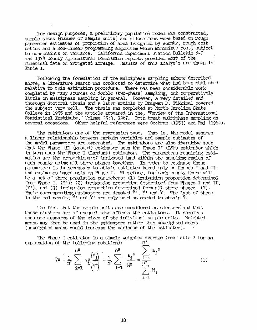
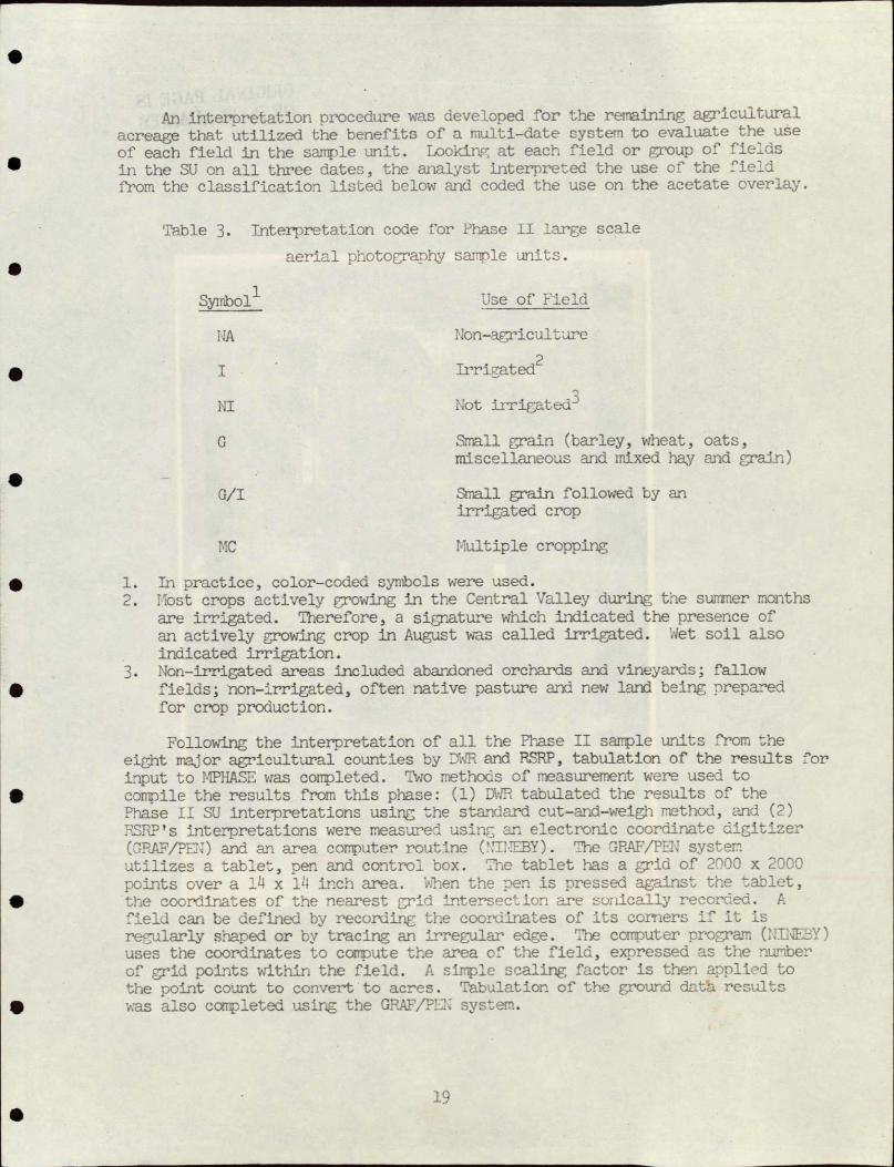
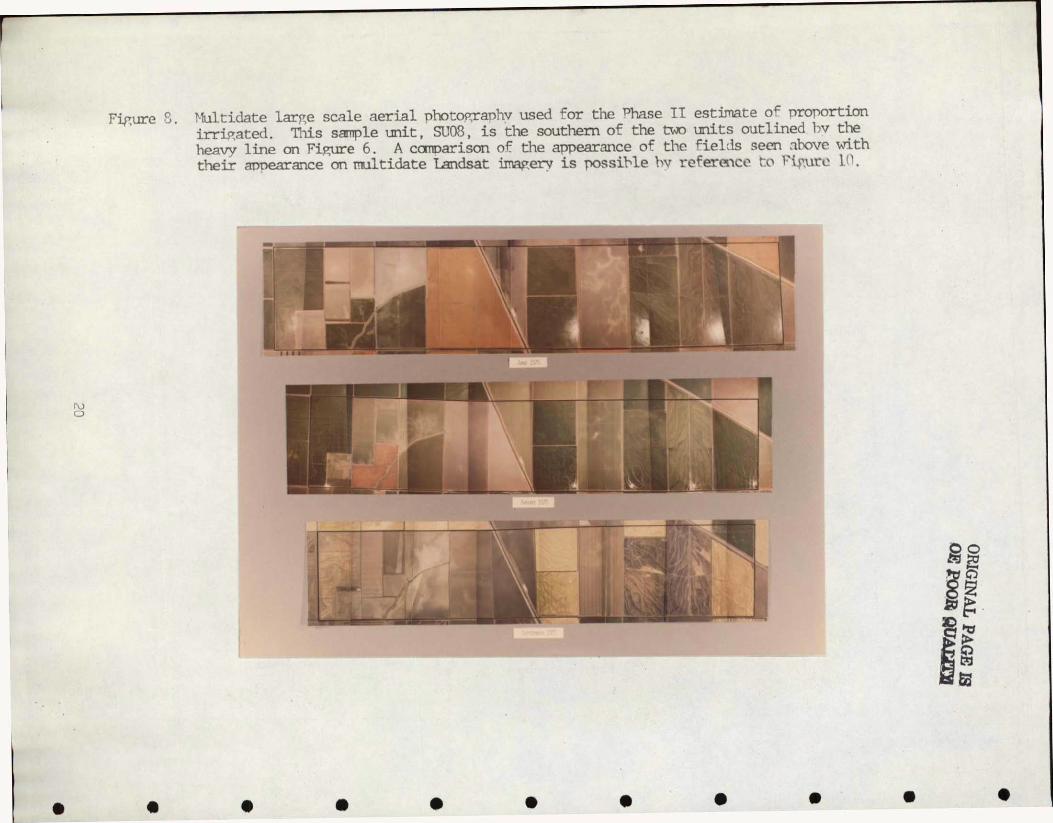
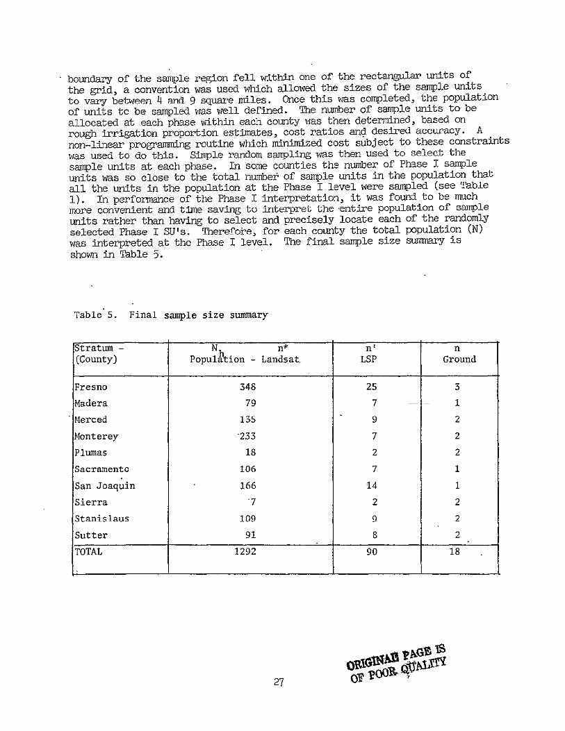
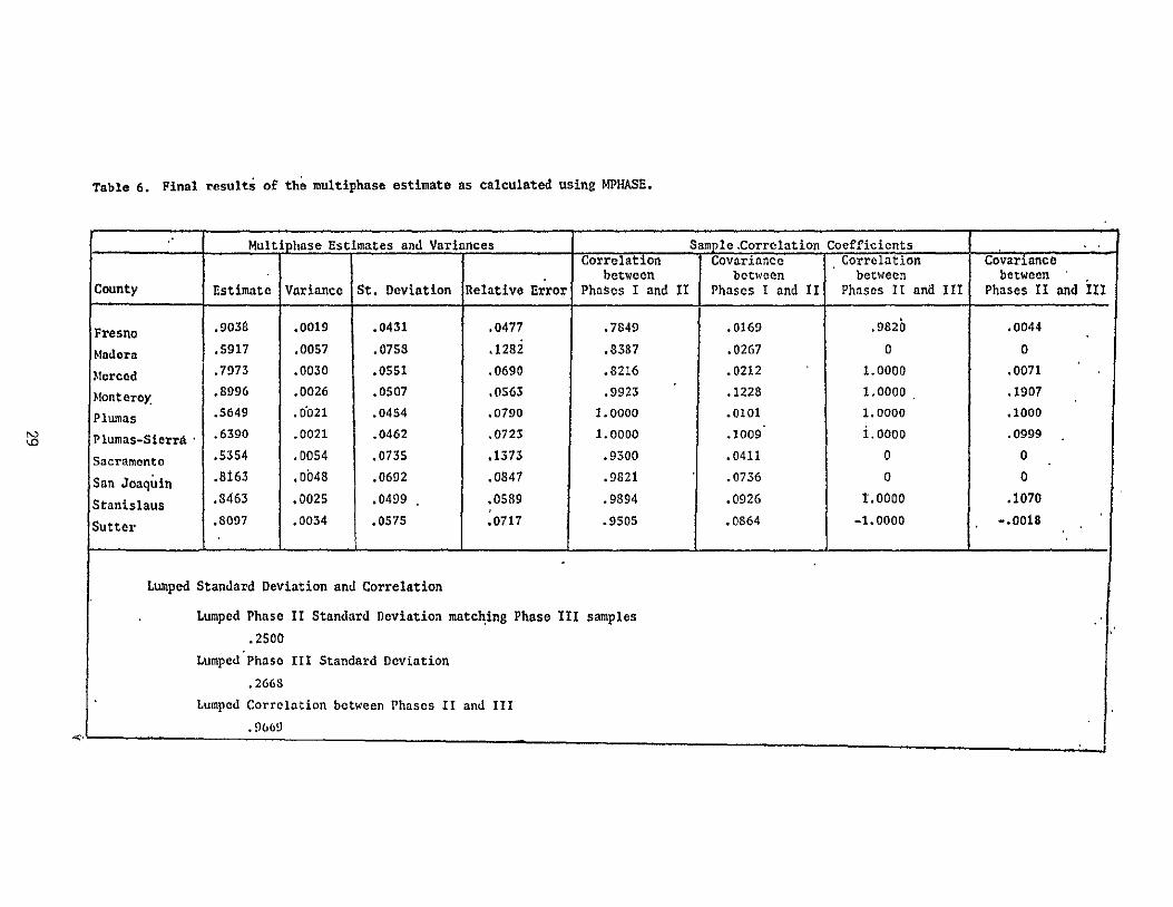
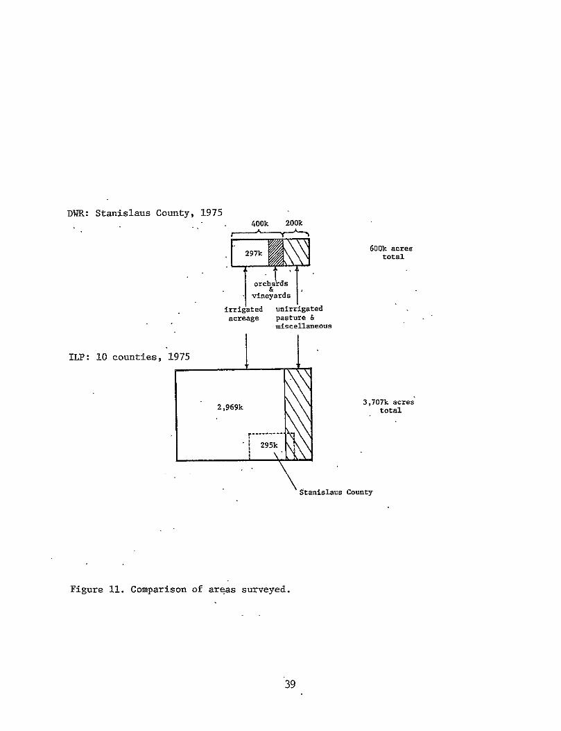
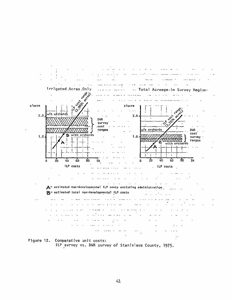
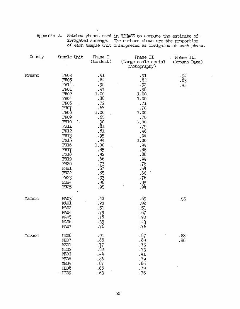

Appendix A Continued
County Sample Unit Phase I (Landsat)
Sutter SU07 SU08 SUOl SU02 SU03 SU04 SU05 SU06
100 73 50 73 57 42 75 98
Phase II Phase III (Large scale aerial- (Ground Data)
photography)
79 98
68 72
59
52
51 140 80 92
52


![[XLS] · Web view317 317 317 317 315 94 315 94 86 86 86 426 426 426 316 239 316 239 317 317 317 315 94 315 94 315 315 315 315 426 274 136 274 136 274 136 274 136 274 188 274 188 274](https://static.fdocuments.in/doc/165x107/5abaa3447f8b9a567c8bbc31/xls-view317-317-317-317-315-94-315-94-86-86-86-426-426-426-316-239-316-239-317.jpg)