Irreversible investment, real options, and competition: Evidence from ...

Journal of Urban Economics 65 (2009) 237–251

Contents lists available at ScienceDirect

Journal of Urban Economics

www.elsevier.com/locate/jue

Irreversible investment, real options, and competition: Evidence from real estatedevelopment

Laarni Bulan a, Christopher Mayer b,c,∗, C. Tsuriel Somerville d

a Brandeis University, International Business School, 415 South Street, MS 021, Waltham, MA 02454, USAb NBER, USAc Columbia Business School, Uris Hall 808, 3022 Broadway, NY, NY 10027, USAd Sauder School of Business, University of British Columbia, 2053 Main Mall, Vancouver, BC V6T 1Z2, Canada

a r t i c l e i n f o a b s t r a c t

Article history:Received 26 October 2007Revised 10 March 2008Available online 12 April 2008

We examine the extent to which uncertainty delays investment, and the effect of competition on thisrelationship, using a sample of 1214 condominium developments in Vancouver, Canada built from 1979–1998. We find that increases in both idiosyncratic and systematic risk lead developers to delay newreal estate investments. Empirically, a one-standard deviation increase in the return volatility reducesthe probability of investment by 13 percent, equivalent to a 9 percent decline in real prices. Increasesin the number of potential competitors located near a project negate the negative relationship betweenidiosyncratic risk and development. These results support models in which competition erodes optionvalues and provide clear evidence for the real options framework over alternatives such as simple riskaversion.

© 2008 Elsevier Inc. All rights reserved.

1. Introduction

Over the last two decades, the application of financial optiontheory to investment in real assets has altered the way that re-searchers model investment.1 Under the real options approach,firms should apply a higher user cost to new investments in ir-reversible assets when returns are stochastic, reflecting the optionto delay that is lost when investment occurs. The effects can bequite large. For example, Dixit and Pindyck (1994) use simulationsto show that the optimal hurdle price triggering new irreversibleinvestment can be two to three times as large as the trigger valuewhen investments are reversible. Yet others argue that competitionerodes option values and limits the empirical relevance of the realoptions framework for many industries. Empirical support for thereal options model has suffered from the absence of a clean test todifferentiate between real options and more traditional discountedcash flow (DCF) models of investment in which the discount ratedepends on risk.

* Corresponding author. Fax: +1 212 854 8776.E-mail addresses: [email protected] (L. Bulan), [email protected]

(C. Mayer), [email protected] (C.T. Somerville).1 Reviews of the theoretical literature include Dixit and Pindyck (1994), Trigeor-

gis (1996), and Brennan and Trigeorgis (2000). Among the seminal papers in thisareas are Abel (1983), Bernanke (1983), Brennan and Schwartz (1985), McDonaldand Siegel (1986), Majd and Pindyck (1987), Pindyck (1988), Dixit (1989), and Abelet al. (1996).

0094-1190/$ – see front matter © 2008 Elsevier Inc. All rights reserved.doi:10.1016/j.jue.2008.03.003

In this paper, we address these issues by examining the re-lationship between uncertainty, competition, and irreversible in-vestment using unique data on 1214 individual real estate projects(condominium or strata buildings) built in Vancouver, Canada be-tween 1979 and 1998. In looking at real estate, we examine anasset class that represents a large component of national invest-ment and wealth and a sector that exhibits great cyclical volatilityin investment.

Some theoretical papers have argued that real options modelshave limited power to predict investment in competitive markets.Caballero (1991) suggests that imperfect competition is vital topredicting a negative relationship between uncertainty and invest-ment. For example, competition might mitigate the value of a realoption through the threat of preemption as in Grenadier (2002).Trigeorgis (1996) associates increased competition with a higherdividend yield from the underlying asset. When the dividend ishigh enough, it can induce early exercise by reducing the value ofthe option to wait. In a similar vein, Kulatilaka and Perotti (1998)argue that firms with a strategic advantage (market power) are ina better position to gain greater growth opportunities when uncer-tainty is higher. This induces more investment in growth optionsfor this type of firm while companies that do not have a strategicadvantage will be discouraged from investing.

In response to these critiques, others argue that with the addi-tion of a few realistic assumptions, the value of the option to waitis preserved even with perfect competition. For example, Novy-Marx (2005) shows that competition does not diminish the valueof an option to develop in the case of differentiated products such

http://www.ScienceDirect.com/

http://www.elsevier.com/locate/jue

mailto:[email protected]



http://dx.doi.org/10.1016/j.jue.2008.03.003

238 L. Bulan et al. / Journal of Urban Economics 65 (2009) 237–251

as real estate where locations are never perfect substitutes for eachother and sites have varying opportunity costs of development dueto differences in the pre-existing use of a site. Leahy (1993) andDixit and Pindyck (1994) also contend that perfect competitiondoes not necessarily reduce the value of waiting.

Existing empirical research supports the existence of a negativerelationship between volatility and investment (Downing and Wal-lace, 2001; Moel and Tufano, 2002; Cunningham, 2006 and 2007).Nonetheless, real options models are not the only models in whichone would expect a negative correlation between uncertainty andinvestment, an issue that is often not discussed in empirical realoptions research. In fact, if increases in volatility are driven by agreater exposure to non-diversifiable risk, most neoclassical mod-els (such as the familiar capital asset pricing model—CAPM) wouldpredict that greater uncertainty would lead to lower investmentthrough an increase in the investor’s required rate of return. Inthe case of incomplete markets, even increases in idiosyncratic riskwill cause risk-averse investors to reduce investment if they cannotadequately hedge this type of risk. This latter condition is espe-cially likely in the context of real estate, where many investorsand developers are small and hold portfolios that are concentratedin a particular local market where they hold great expertise, butwhere there are no existing methods to hedge local market risk.Our findings described below address both of these issues.

We find clear support for the negative relationship between id-iosyncratic uncertainty and investment that is a crucial predictionof the real options model. To separate the impact of the alter-native models, real options and the CAPM, we decompose thevolatility of condominium returns into idiosyncratic and marketrisk components. As predicted by the real options model, exposureto idiosyncratic risk reduces investment. However, consistent withthe CAPM, exposure to market volatility also delays investment tonearly the same extent. A one standard deviation increase in id-iosyncratic volatility reduces the probability of development by 13percent, about the same predicted impact on new investment as a9 percent decrease in real prices. A similar one standard deviationincrease in market volatility reduces the likelihood of investmentby the equivalent to a 7 percent fall in real prices.

Addressing the debate about how market structure impacts op-tion exercise, we show that competition, measured by the numberof potential competitors for a project, reduces the impact of condoreturn volatility on new investment. Empirically, competition haslittle direct effect on investment. Instead, competition only mat-ters when interacted with volatility. We show that volatility hasa smaller impact on option exercise for developments surroundedby a larger number of potential competitors. In fact, for the 5 per-cent of all units facing the greatest number of potential competi-tors, idiosyncratic volatility has virtually no effect on the timing ofinvestment. These findings provide unambiguous support for themodels of Caballero, Trigeorgis and Grenadier, which show thatcompetition can erode the value of the option to delay irreversibleinvestment.

Finally, the finding that competition only impacts investmentindirectly through its correlation with uncertainty provides sup-port for the real options model even in the presence of risk averseowners and incomplete markets. While risk averse owners with-out hedging opportunities will reduce investment in response togreater idiosyncratic volatility, only a real options model has theadditional prediction that option value diminishes with competi-tion.

The relationship between competition and real option exercisemay help explain the strong pro-cyclical correlation between in-vestment and output. Macro economists have often puzzled overthe high volatility of investment relative to output, documentedover long periods of time and across many countries (Basu andTaylor, 1999). Variation in competition over the cycle could pro-

vide at least one explanation for the excess volatility of invest-ment. Rotemberg and Saloner (1986) and Rotemberg and Wood-ford (1991, 1992) argue that tacit collusion is difficult to sustainin booms, relative to busts. Our findings suggest that variation incompetition can impact investment. Firms might optimally furtherdelay investment in busts when product markets are less compet-itive, but undertake equivalent investments in booms when theyface greater competition. This higher volatility for investment isconsistent with the macro evidence.

The remainder of the paper is structured as follows. Section 2provides a review of related work and a discussion of how this pa-per fits in with the empirical real options literature. In Section 3,we present the empirical specification along with a summary ofits theoretical support. We also discuss the impact of various as-sumptions on the specification with respect to the completeness ofcapital markets and the unique properties of the real estate mar-ket. We present a more detailed discussion of the data in Section 4.The empirical results are presented in Section 5, and in Section 6we conclude.

2. Existing literature

Real options theory has been applied to describe a broad rangeof investments and industries.2 Macroeconomic aggregate studiesby Pindyck and Solimano (1993) and Caballero and Pindyck (1996)find a negative relationship between aggregate investment and un-certainty, where uncertainty is measured as the variance in themaximum observed marginal revenue product of capital. Other pa-pers (Holland et al., 2000; Sivitanidou and Sivitanides, 2000; Singand Patel, 2001; and Cunningham, 2006 and 2007) examine thisrelationship specifically for real estate development, and usually,but not always, find a negative relationship between uncertaintyand development. Leahy and Whited (1996) and Bulan (2005) alsoobtain mixed results when examining the effect of a firm’s dailystock return volatility on the firm-level investment-capital stockratio for a panel of manufacturing firms. However, real optionsmodels apply most directly to individual investment projects andpredict that trigger prices are non-linear, so aggregate investmentstudies may obscure these relationships.

Studies that use project level investment data have the ad-vantage of being able to relate individual investment decisionsto direct measures of demand uncertainty such as output pricevolatility.3 These papers have sometimes found limited evidenceof a link between investment and volatility (e.g., Hurn and Wright,1994), although recent work has tended to be more supportive ofreal options. Bell and Campa (1997) demonstrate that the volatilityof exchange rates has a negative effect on new capacity invest-ment in the international chemical industry, but that the volatilityof input prices and demand have small and insignificant effects.Downing and Wallace (2001) find a negative link between volatilityof prices and costs and the decisions of homeowners to improvetheir homes. Moel and Tufano (2002) examine the determinants ofthe decision to close or re-open a mine using a sample of 285 goldmines. They find that gold price volatility has a negative and sta-tistically significant effect on these decisions, but that factors suchas firm-specific managerial decisions also matter.

We take advantage of micro-data on a large number (1214) ofcondominium developments and examine the impact of volatility

2 Applications include investments in natural resources extraction (Brennan andSchwartz, 1985; Paddock et al., 1988), patents and R&D (Pakes, 1986), and real es-tate (Titman, 1985; Wiliams, 1991, 1993; and Grenadier, 1996). Lander and Pinches(1998) summarize the applied literature.

3 Quigg (1993) takes a different approach. She develops a structural model of landvaluation using data in Seattle, finding that the option to wait is worth about 6percent of the value of undeveloped industrial land, a relatively low value.

L. Bulan et al. / Journal of Urban Economics 65 (2009) 237–251 239

using relatively disaggregated neighborhood output (condominium)prices in an approach that is similar to Moel and Tufano (2002)and Cunningham (2006 and 2007). Moel and Tufano use detaileddata on the operating and maintenance costs for mines and theconvenience yield (rental value) of gold to estimate a reduced-form probit model of the determinants of opening and closinga mine. Their strength is in the detailed data on costs and con-venience yield and the precise measurement of mine openingand closing. In this paper we use the same basic methodology,a reduced-form hazard model. Yet we focus on price volatility in-stead of cost volatility for the following reasons: First, volatility inconstruction cost components such as wages and materials rep-resent a relatively small portion of the variability in the profitsof builders relative to the volatility of selling prices. Second, in-terest rates are more important for developers, but the impact ofinterest rate volatility cannot be reliably disentangled from pricevolatility. Third, we can use neighborhood price indexes to ob-tain cross-sectional and time-series variation in price volatility, butwe only have aggregate data on costs. Fourth, work by Somerville(1999) indicates that construction cost indexes perform poorly inmodels of housing supply, because of errors in index constructionand the endogeneity between housing starts and local unobservedcosts.

Cunningham (2006) implements a similar model to ours us-ing data from the Seattle metro area. The paper shows that a onestandard deviation in volatility reduces development by 11.3 per-cent, similar to our estimates, below. The paper goes on to showthat uncertainty has the biggest effect on construction at the urbanfrontier. Subsequently, Cunningham (2007) shows that regulationsthat have the impact of reducing uncertainty diminish the impactof regulation in reducing new construction.

However, our study provides some important enhancements toprevious studies. This is the first study of real options and invest-ment that we know of that differentiates between the impact ofsystematic (market) and non-systematic risk. In addition, we ex-amine the prediction that the extent of competition can mitigatethe negative relationship between uncertainty and investment. Byquantifying different types of risk and also the extent of compe-tition, we hope to exploit those factors present in a real optionscharacterization, but not in more standard discounted cash flow orCAPM investment frameworks. This allows us to differentiate be-tween effects found in a real options model from simply observingthat uncertainty negatively impacts development, a prediction notunique to real options models.4 Evidence that competition dimin-ishes the relationship between investment and idiosyncratic riskwould support a real options interpretation because it is difficultto find a comparable prediction in a model of risk aversion thatdoes not rely on real options behavior.

One potential complication is that our data contain a mix oflarge national developers and medium and small-sized local de-velopers. We cannot explicitly identify the developers of individualprojects from the data, as most developments, even those by largepublic developers, are typically done by wholly-owned shell com-panies, one per development. Evidence from other work indicatesthat the vast majority are small and medium-sized local develop-ers, with some national developers and individual developers fromAsia.5 Clearly these various types of developers may react differ-

4 Systematic risk is predicted to reduce investment in a variety of models (includ-ing the CAPM) via the cost of capital where non-systematic risk is not priced. Realoptions models predict a negative impact of non-systematic risk on investment. Anunobserved investment-specific discount rate that is correlated with aggregate un-certainty will yield a negative relationship between volatility and investment, butwould be insufficient to prove real options behavior.

5 75 percent of projects in a larger sample of developments in the Vancouvermetropolitan area were constructed by developers who built fewer than 13 projectsbetween 1970 and 2002.

ently to idiosyncratic risk. Risk aversion on the part of small de-velopers might lead them to delay investment if they cannot hedgethe risk, which must be true for local (Vancouver) real estate pricerisk. Our results regarding competition are quite important in thisregard, as they are direct predictions from real options models thatdo not arise from the traditional DCF investment models and can-not easily be tied to risk aversion by small local developers whomight hold undiversified portfolios.

3. Empirical specification

We begin by characterizing some of the basic features of thestandard, partial-equilibrium real options model to convey someintuition. We then discuss issues specific to the real estate marketthat may alter the forces at work in this simple framework. Weconsider how these issues may change the standard predictions,and how we try to address them in our empirical analysis.

Most real options models solve for the price level that triggersnew investment, P∗ , so that when P > P∗ , the owner will chooseto make an irreversible investment. In the simplest form of themodel, the only source of uncertainty is the path of future assetprices6 and investments are completely irreversible, thus ignoringthe put option to sell for an alternative use. The asset price evolvesas a geometric Brownian motion process:

dP/P = α dt + σ dz (1)

where α and σ 2 are the drift (expected capital appreciation) andvariance parameters, respectively, and dz is the increment of aWiener process. The asset is also assumed to have a constant, con-venience (dividend) yield δ. A closed form solution can be found bydynamic programming or contingent claims pricing, assuming thatthere are securities in the economy that span the risk in P .7 Asin the familiar option pricing formula of Black and Scholes (1973),the trigger price is:

P∗ = f (μ+, δ−, σ+), (2)

where f is a non-linear function, μ is the discount rate (equivalentto the expected rate of return on the asset), and the superscriptsign represents the expected sign of the effect of an increase ineach of these parameters on P∗ . The usual comparative static re-sults from option pricing theory apply: the trigger price for newinvestment is increasing in the discount rate, increasing in thevolatility of returns and decreasing in the convenience yield.8

The specification for the discount rate depends on the assump-tions regarding risk preferences and complete markets. If investorsare risk-neutral the discount rate is the risk-free rate of return,usually assumed to be the interest rate on a short-term govern-ment security. Alternatively, if investors are risk-averse but marketsare complete, the return on an asset can be derived from the cap-ital asset pricing model (CAPM):

μ = r f + φρpmσ . (3)

Here r f is the risk-free rate of return, φ is the market price ofrisk, σ is the standard deviation of the excess returns on the asset,

6 Williams (1991) and Quigg (1993), for example, assume cost uncertainty in ad-dition to price uncertainty. In Grenadier (1996, 2002) and Novy-Marx (2005), it isthe underlying demand shock that follows a geometric Brownian motion process.Consequently, the endogenously derived price process evolves as a reflected Brow-nian motion that is affected by aggregate supply in addition to the demand statevariable.

7 Quigg (1993), for example, assumes that there exists an equilibrium in whichcontingent claims on both building prices and development costs are priceduniquely. See Dixit and Pindyck (1994) for more detail on these models.

8 Ideally, we would be able to observe the exact determinants of all factors thatdetermine P∗ , including the cost of development and profitability at each site foreach point in time, enabling structural estimation of f . Unfortunately, such variablesare difficult to obtain.


and ρpm is the correlation between excess returns on the asset,in our case real estate, and excess returns for the broader market.Finally, if markets are in equilibrium but are incomplete and in-vestors are risk averse, we can use a project specific discount rate,ρ , as the sum of expected capital appreciation and the convenienceyield, as follows:

ρ = α + δ. (4)

In the empirical work, it is important to properly control forthe discount rate, since volatility might reduce the likelihood of in-vestment not because of real options behavior, but instead becauseinvestors or real estate developers are risk averse and volatilityenters the discount rate directly. For example, in the CAPM, sys-tematic risk reduces the likelihood of investment, not due to anyeffect of irreversible investment, but instead because investors can-not fully hedge systematic or market risk. Below, we choose toinclude several alternative proxies for the (unobserved) discountrate, including estimates of the risk-free rate, the CAPM discountrate, and a project-specific discount rate derived from the relation-ship in Eq. (4). With incomplete markets for real estate assets andmany individual investors who are likely risk averse, we would ex-pect that risk factors will play a role. So, for example, the discountrate (μ) should depend, at least in part, on the covariance betweenthe volatility of local real estate prices and aggregate risk, as in theCAPM.

The traditional model described above assumes that prices fol-low geometric Brownian motion with a constant drift and variance.However, existing empirical work strongly suggests that real estateprices exhibit short-run positive serial correlation and long-runmean reversion.9 In addition, the volatility of asset returns havebeen shown to vary over time. Yet even when the random walkassumption is relaxed and the volatility of returns is taken to bestochastic, assumptions which more closely replicate the circum-stances in our data, the qualitative predictions of the model stillhold. For example, Heston (1993) derives a closed-form solutionfor pricing options in a model with time-varying stochastic volatil-ity. He finds that, similar to Black and Scholes (1973), a highervariance still increases the price of an option.10 When both meanreverting interest rates and the convenience yield are stochastic,Miltersen (2000) finds similar qualitative effects, but with a loweroption value than in the standard Black–Scholes (1973) framework.Schwartz (1997) uses numerical methods to obtain comparativestatics for a model with stochastic factors in mean reverting prices,mean reverting convenience-dividend- yields and time-varying in-terest rates. Even in this more complicated world, the usual realoptions results hold, with the exception that option values becomeless sensitive to prices when there is mean-reversion in prices.Finally, Lo and Wang (1995) show that with auto-correlation inreturns, the option-pricing formula is unchanged.11 All of thesefindings suggest that the usual real options prediction that the in-vestment trigger price increases with uncertainty would still applyto the real estate market.

In models such as Williams (1991), Quigg (1993), and Dixit andPindyck (1994), costs play an important role in determining thetrigger price for investment. Assuming that the cost process fol-lows geometric Brownian motion, P∗ would be increasing in bothcosts and cost volatility. For the reasons outlined earlier, we ignorethe volatility of costs and focus instead on prices.

9 See Case and Shiller (1989), Meese and Wallace (1993), and Quigley and Red-fearn (1999).10 The stochastic volatility assumption affects the kurtosis and skewness in the

distribution of spot returns.11 They show that if the unconditional variance of returns is held constant,

changes in the predictability of returns implies that the diffusion coefficient mustalso change over time.

Without detailed cost data and the ability to properly estimatebuilder profits and thus a specific hurdle rate for prices, P∗ , ourempirical approach is to identify the principal implication of highertrigger prices, i.e. that investment is delayed. Below, we look at thetime from an arbitrary starting point (January 1979) until develop-ment occurs. Explicitly, we estimate the hazard rate of investmenth(t), defined as the conditional probability of development occur-ring at time t , as:

h(t) = Pr(

Pt � P∗t | Px < P∗

x ,∀x < t). (5)

Given the current price level, the hazard rate is decreasing in theprice trigger P∗ . We can therefore estimate a reduced form hazardspecification, where the hazard rate is a function of the determi-nants of P∗ , holding the current price level fixed. The hazard hasthe following empirical specification:

h(t) = exp(

X ′tβ

)h0(t), (6)

where Xt is a vector of explanatory variables and β is the vector ofcoefficients to be estimated. As described in more detail below, weallow the price level and the volatility of condo returns to changeover time. The base model assumes a Weibull distribution for t;that is, the baseline hazard rate, h0, is monotonically increasingor decreasing over time.12 We examine alternative distributions aswell in the empirical results that follow.

4. Data description

We use data on all strata (or condominium) projects with atleast four units per project built in the city of Vancouver, Canadabetween January 1979 and February 1998—a total of 1297 projects.Projects are identified according to the date that the governmentresponds to the developer’s filing of a strata plan to convert thesingle title for the land into multiple strata (condominium) titles.13

By law this can only occur near the completion of construction. Weconvert the granting of a strata title to the start of construction byintroducing a one-year lag in the dependent variable.14

Over this period there are several bursts of development ac-tivity. Fig. 1 shows four peaks in the number of strata real estateprojects in 1982, 1986, 1991, and 1996. In addition, there has beena large secular increase in the average project size. The increasein condominium development activity over this time period wasmuch greater than the growth in single family construction, bothin the City of Vancouver, because of an absence of undevelopedland, and even in the metropolitan area. Local commentators de-scribe the mid-1980s as the point at which a broad, general ac-ceptance of the strata form of ownership began, so that over thisperiod the growth in strata projects exceeded that of single familydevelopments.

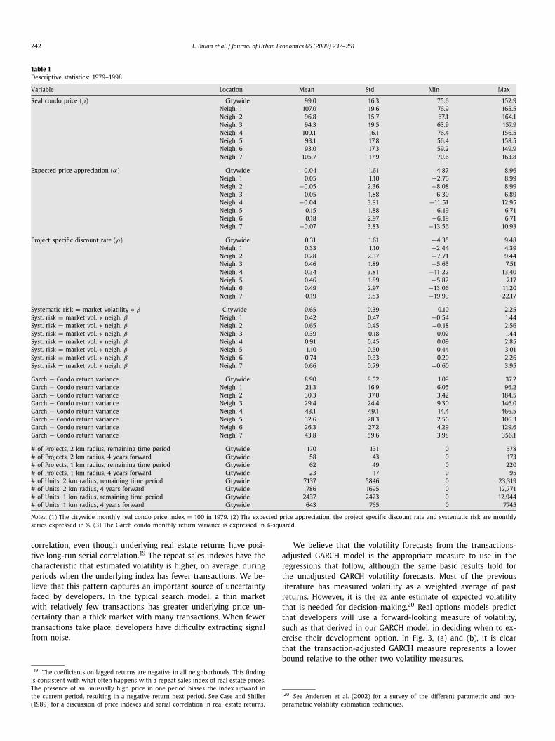
Table 1 presents the descriptive statistics for the monthly dataused in the paper, including citywide and neighborhood prices, thevolatility of returns, expected price appreciation, the project spe-cific discount rate, systematic risk, and the extent of competition

12 Under the Weibull specification, h0(t) = pt p−1. If p > 1, then the baseline haz-ard rate is monotonically increasing, if p < 1, the baseline hazard is monotonicallydecreasing, and if p = 1, the baseline hazard is a constant (which is equivalent toan exponential distribution for t).13 In British Columbia condominium units are those with a strata title to allocate

ownership of the land among the units. Strata title legislation was first enactedin British Columbia in September 1966 and the first units under this legal formwere built in 1968. While non-residential strata-titles exist, over 95 percent of strataprojects are residential. For a discussion of strata title legislation and the first yearsof strata development in British Columbia, see Hamilton (1978).14 Nearly all real estate development is primarily debt financed. Lenders have

strong incentives to ensure that construction occurs as expeditiously as possible,which is reflected in the loan terms. Developer equity is the first in and last out.Consequently, assuming an exogenous lag is not unreasonable, as there is little in-centive to delay construction.


Fig. 1. Vancouver condominium projects.

across projects. The construction of these variables is described be-low. All data are presented in real terms.15

We compute monthly repeat sales indexes of condominiumprices, using data obtained from the British Columbia Assess-ment Authority (BCAA) of all condominium transactions from 1979to 1998. A repeat sales index has the advantage of controlling forchanges in the quality of aggregate characteristics of units soldover time because it is composed of the change in the prices ofindividual units and is not a market average.16 We create sep-arate price indexes for seven sections of the city according toBCAA neighborhood boundaries using the geometric repeat salesmethodology outlined in Shiller (1991). Three neighborhoods areunique while the other four are amalgamations that are geo-graphically contiguous, demographically similar, and have suffi-cient transactions to create a monthly price index. We exclude 83projects in neighborhoods that are difficult to combine into homo-geneous sub-markets, leaving a total sample of 1214 units.

Although we use neighborhood price indexes in all of the re-gressions that follow, Fig. 2 presents the city-wide real price indexfor Vancouver condominiums. Our period of analysis covers threeclear real estate price cycles. The first is a striking run-up be-tween mid-1980 and mid-1981 followed by a sharp fall endingin mid-1982. The second is the 1988–1990 increase in prices thatcoincided with the post-Tiananmen Square wave of immigrationfrom Hong Kong. The third is the much more moderate 1991–1994period of increasing prices. Between 1994 and 1998, real condo-minium prices in Vancouver fell approximately 15 percent.

To measure uncertainty, we compute a time-varying measureof the volatility of monthly neighborhood returns. First, we use anautoregressive model of returns on lagged returns to predict futurereal estate returns. We then apply a GARCH (1,1) model to esti-mate the variance of the residuals from the first stage prediction.

15 We deflate with the moving average of the monthly inflation rate for the previ-ous 6 months with declining weights by month.16 These condominium data are less susceptible to some of the flaws of repeat

sales indexes. First, it is very hard to add to or substantially renovate these units,so unit quality and quantity are more likely to remain constant over time. Sec-ond, these units transact more frequently than do single family units, so we discardfewer transactions when requiring that units used for the repeat sales index mustsell at least twice over the sample period. See Thibodeau (1997) for a summary ofthe issues associated with computing real estate price indexes.

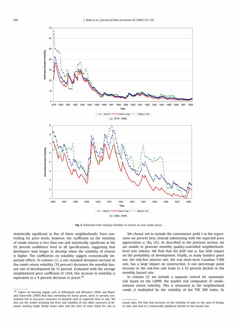
This GARCH specification incorporates the serial correlation in re-turns and time-varying volatility discussed in the previous section,which is more appropriate to real estate prices than geometricBrownian motion. Using conditional maximum-likelihood, we ob-tain estimates of the conditional variance of monthly neighborhoodreturns given past prices, while controlling for the predictabil-ity in returns. The structure imposed by the GARCH model willnot change the qualitative predictions of the real options model:Bollerslev et al. (1992) maintain that the simple structure imposedby the GARCH model can be viewed as a reduced form of a morecomplicated dynamic process for volatility.17

We also consider two additional measures of uncertainty. Thefirst is the simple variance in monthly neighborhood returns overthe previous two years. The second is the same GARCH specifi-cation described above, but with a correction for the componentof volatility caused by differences in the ratio of repeated salesof the same unit to the total transactions in a month. In using arepeat sales index, we include those transacting units for whichthere is at least one additional transaction in the sample. How-ever, we expect a developer to make an assessment based on alltransactions in the market.18 The three series of monthly returnvolatilities are presented for the city-level in Fig. 3, (a) and (b), for1979–1998 and for the sub-period 1986–1998, respectively. Returnvolatilities are substantially lower in the 1986 to 1998 period be-cause we exclude the 1981 price spike and the period at the startof the sample where total volume of transactions is low because ofthe small number of condominium units. The volatility series foreach of the seven neighborhoods displays these same characteris-tics as well.

The appendix table (Table A1) shows the results of the GARCHestimation using transactions-adjusted returns. The coefficients onlagged returns provide evidence of short horizon negative serial

17 Heston and Nandi (2000) show that a more general form of the GARCH (1,1)process approaches the stochastic volatility model of Heston (1993) in the continu-ous time limit.18 We correct for this potential bias by scaling mean returns to zero and then mul-

tiplying the calculated return for a given month by the square root of the ratio ofrepeat sales transactions to total transactions. The adjusted GARCH measure effec-tively smooths volatility as the share of sales in the repeat data base falls, offsettinga higher measured variance in months where we have relatively fewer repeat sales.We thank Robert Shiller for pointing out this issue and suggesting this correction.


Table 1Descriptive statistics: 1979–1998

Variable Location Mean Std Min Max

Real condo price (p) Citywide 99.0 16.3 75.6 152.9Neigh. 1 107.0 19.6 76.9 165.5Neigh. 2 96.8 15.7 67.1 164.1Neigh. 3 94.3 19.5 63.9 157.9Neigh. 4 109.1 16.1 76.4 156.5Neigh. 5 93.1 17.8 56.4 158.5Neigh. 6 93.0 17.3 59.2 149.9Neigh. 7 105.7 17.9 70.6 163.8

Expected price appreciation (α) Citywide −0.04 1.61 −4.87 8.96Neigh. 1 0.05 1.10 −2.76 8.99Neigh. 2 −0.05 2.36 −8.08 8.99Neigh. 3 0.05 1.88 −6.30 6.89Neigh. 4 −0.04 3.81 −11.51 12.95Neigh. 5 0.15 1.88 −6.19 6.71Neigh. 6 0.18 2.97 −6.19 6.71Neigh. 7 −0.07 3.83 −13.56 10.93

Project specific discount rate (ρ) Citywide 0.31 1.61 −4.35 9.48Neigh. 1 0.33 1.10 −2.44 4.39Neigh. 2 0.28 2.37 −7.71 9.44Neigh. 3 0.46 1.89 −5.65 7.51Neigh. 4 0.34 3.81 −11.22 13.40Neigh. 5 0.46 1.89 −5.82 7.17Neigh. 6 0.49 2.97 −13.06 11.20Neigh. 7 0.19 3.83 −19.99 22.17

Systematic risk = market volatility ∗ β Citywide 0.65 0.39 0.10 2.25Syst. risk = market vol. ∗ neigh. β Neigh. 1 0.42 0.47 −0.54 1.44Syst. risk = market vol. ∗ neigh. β Neigh. 2 0.65 0.45 −0.18 2.56Syst. risk = market vol. ∗ neigh. β Neigh. 3 0.39 0.18 0.02 1.44Syst. risk = market vol. ∗ neigh. β Neigh. 4 0.91 0.45 0.09 2.85Syst. risk = market vol. ∗ neigh. β Neigh. 5 1.10 0.50 0.44 3.01Syst. risk = market vol. ∗ neigh. β Neigh. 6 0.74 0.33 0.20 2.26Syst. risk = market vol. ∗ neigh. β Neigh. 7 0.66 0.79 −0.60 3.95

Garch − Condo return variance Citywide 8.90 8.52 1.09 37.2Garch − Condo return variance Neigh. 1 21.3 16.9 6.05 96.2Garch − Condo return variance Neigh. 2 30.3 37.0 3.42 184.5Garch − Condo return variance Neigh. 3 29.4 24.4 9.30 146.0Garch − Condo return variance Neigh. 4 43.1 49.1 14.4 466.5Garch − Condo return variance Neigh. 5 32.6 28.3 2.56 106.3Garch − Condo return variance Neigh. 6 26.3 27.2 4.29 129.6Garch − Condo return variance Neigh. 7 43.8 59.6 3.98 356.1

# of Projects, 2 km radius, remaining time period Citywide 170 131 0 578# of Projects, 2 km radius, 4 years forward Citywide 58 43 0 173# of Projects, 1 km radius, remaining time period Citywide 62 49 0 220# of Projects, 1 km radius, 4 years forward Citywide 23 17 0 95# of Units, 2 km radius, remaining time period Citywide 7137 5846 0 23,319# of Units, 2 km radius, 4 years forward Citywide 1786 1695 0 12,771# of Units, 1 km radius, remaining time period Citywide 2437 2423 0 12,944# of Units, 1 km radius, 4 years forward Citywide 643 765 0 7745

Notes. (1) The citywide monthly real condo price index = 100 in 1979. (2) The expected price appreciation, the project specific discount rate and systematic risk are monthlyseries expressed in %. (3) The Garch condo monthly return variance is expressed in %-squared.

correlation, even though underlying real estate returns have posi-tive long-run serial correlation.19 The repeat sales indexes have thecharacteristic that estimated volatility is higher, on average, duringperiods when the underlying index has fewer transactions. We be-lieve that this pattern captures an important source of uncertaintyfaced by developers. In the typical search model, a thin marketwith relatively few transactions has greater underlying price un-certainty than a thick market with many transactions. When fewertransactions take place, developers have difficulty extracting signalfrom noise.

19 The coefficients on lagged returns are negative in all neighborhoods. This findingis consistent with what often happens with a repeat sales index of real estate prices.The presence of an unusually high price in one period biases the index upward inthe current period, resulting in a negative return next period. See Case and Shiller(1989) for a discussion of price indexes and serial correlation in real estate returns.

We believe that the volatility forecasts from the transactions-adjusted GARCH model is the appropriate measure to use in theregressions that follow, although the same basic results hold forthe unadjusted GARCH volatility forecasts. Most of the previousliterature has measured volatility as a weighted average of pastreturns. However, it is the ex ante estimate of expected volatilitythat is needed for decision-making.20 Real options models predictthat developers will use a forward-looking measure of volatility,such as that derived in our GARCH model, in deciding when to ex-ercise their development option. In Fig. 3, (a) and (b), it is clearthat the transaction-adjusted GARCH measure represents a lowerbound relative to the other two volatility measures.

20 See Andersen et al. (2002) for a survey of the different parametric and non-parametric volatility estimation techniques.


Fig. 2. Vancouver condominium monthly real price index.

We compute expected price appreciation, α, from an auto-regressive process up to order three for each of the neighborhoodreturn series. Expected price appreciation (the drift rate) is the onemonth ahead return forecast from this specification. The projectspecific discount rate, ρ , is defined as the sum of expected priceappreciation, α, and the monthly dividend yield, δ, as in Eq. (4).The dividend yield is derived from a combination of our price in-dexes and the CMHC (Canada Mortgage Housing Corporation) rentsurveys.21

Finally, we measure exposure to market volatility, as in theCAPM, by multiplying the monthly Toronto Stock Exchange (TSE)300 market return volatility22 by a time varying measure of theCAPM β , the covariance between excess returns in the Vancouvercondo market and the TSE 300. Most studies of the stock marketalso show that individual stock β ’s appear to change over time.To estimate a time varying measure of beta we use Cleveland andDevlin’s (1988) locally weighted regression methodology. This non-parametric specification estimates β using a weighted sub-sampleof the time series, with heaviest weights on the closest time peri-ods (Fig. 4).23

5. Empirical results

The hazard model in Eq. (6) is estimated by maximum likeli-hood. The baseline hazard rate, h0, reflects the probability of de-velopment as a function of time alone. The explanatory variableswill affect the probability of development multiplicatively by thefactor eβ . The null hypothesis of β = 0 corresponds to a coefficientof 1 in the hazard model. Hence, in the regressions that follow, thecoefficient on a variable X that we estimate is the proportionaleffect on the hazard rate of a unit change in X . An estimated co-efficient greater than one in the regression output suggests that

21 We use cross-sectional rent levels from the annual CMHC rental survey andneighborhood specific prices from our data to fix a neighborhood specific dividendyield. The price component of this yield then varies over time with our neighbor-hood repeat-sales price indexes, while the rent component varies with the StatisticsCanada metropolitan area rent index (neighborhood specific rents are only availablefor part of our analysis period and then only on an annual or semi-annual basis).22 TSE 300 return volatilities are calculated using a GARCH(1,1) model.23 For each month, the excess neighborhood returns are regressed against excess

TSE 300 returns using the nearest 60% of months in the sample. These observationsare weighted using a tri-cubic function so that the weight for a month declines withdistance in time from the month for which we are estimating the beta.

an increase in the variable has a positive impact on the baselinehazard—that is, a higher probability of development—while a co-efficient less than unity implies the reverse effect.24 We estimateheteroskedasticity-consistent standard errors that allow for corre-lation across time in the hazard rate of individual projects (theHuber/White estimator of variance clustered on each individualproject).

One complication is that we do not observe the start date forconstruction. When the developer files a strata plan, the buildingis almost completed and ready for sale. However, the actual invest-ment (option exercise) takes place months earlier when the devel-oper begins physical construction of the project. To compensate,the date of our dependent variable is lagged by one year to re-flect the time required for physical construction. Somerville (2001)shows that 59 percent of new multi-family projects are completedwithin one year of the start of construction. This built-in lag alsoreduces or eliminates any possible problems relating to simultane-ity between prices and new construction. Reducing the lag lengthto six or nine months has little impact on the results. To controlfor differences in construction time, we include linear, quadraticand cubic terms for project size and dummy variables for buildingtype in the regressions.

5.1. Base specification

The first three columns in Table 2 present maximum likeli-hood estimates of our base specification with the three alterna-tive measures of the project discount rate, μ. All regressions useneighborhood-level price indexes and volatilities, building type andproject size variables and neighborhood fixed effects.25 The re-gression coefficients are generally of the expected sign for thereal options model and are almost uniformly statistically differentfrom one. Not surprisingly, developers choose to develop a parcelmore quickly when neighborhood prices are higher. Price coeffi-cients are greater than one in six of the seven neighborhoods and

24 In the regressions below, a one unit change in X leads to a (eβ − 1) percentchange in the hazard rate. For example, a coefficient of 1.05 implies that a one unitchange in X increases the probability of development by 5%.25 We estimated the model with neighborhood fixed effects at the most disaggre-

gated level (according to the BCAA classification) to incorporate more heterogeneityinto the model without sacrificing too many degrees of freedom. The results aresimilar (with mostly higher z-statistics) to those reported here.


(a) 1979–1998.

(b) 1986–1998.

Fig. 3. Estimated time varying volatility of returns on real condo prices.

statistically significant in five of those neighborhoods. Even con-trolling for price levels, however, the coefficient on the volatilityof condo returns is less than one and statistically significant at the95 percent confidence level in all specifications, suggesting thatdevelopers wait longer to develop when the volatility of returnsis higher. The coefficients on volatility suggest economically im-portant effects. In column (1), a one standard deviation increase inthe condo return volatility (35 percent) decreases the monthly haz-ard rate of development by 13 percent. Evaluated with the averageneighborhood price coefficient of 1.014, this increase in volatility isequivalent to a 9 percent decrease in prices.26

26 Papers on housing supply such as DiPasquale and Wheaton (1994) and Mayerand Somerville (2000) find that controlling for house prices, starts or permits con-sistently fall in non-price measures of demand such as expected time to sale. Wealso run the model including the level and volatility of two other measures of de-mand, existing single family home sales and the ratio of units listed for sale to

We choose not to include the convenience yield δ in the regres-sions we present here, instead substituting with the expected priceappreciation α (Eq. (4)). As described in the previous section, weare unable to generate monthly quality-controlled neighborhood-level rent indexes. We find that the drift rate α, has little impacton the probability of development. Finally, as many builders pointout, the risk-free interest rate, the real short-term Canadian T-Billrate, has a large impact on construction. A one percentage pointincrease in the risk-free rate leads to a 52 percent decline in themonthly hazard rate.

In column (2) we include a separate control for systematicrisk based on the CAPM, the market risk component of condo-minium return volatility. This is measured as the neighborhoodcondo β multiplied by the volatility of the TSE 300 index. As

actual sales. We find that increases in the volatility of sales or the ratio of listingsto sales also lead to a statistically significant decline in the hazard rate.


Fig. 4. Non-parametric β: Vancouver condos vs. TSE300.

Table 2Hazard specification: time to develop a new site

Hazard is estimated using a Weibull distribution

Variable Reg. (1) Reg. (2) Reg. (3) Reg. (4)

Real condo price − neigh. 1 0.9997 1.0021 1.0007 1.0020−(0.11) −(0.60) −(0.18) −(0.58)

Real condo price − neigh. 2 1.0075* 1.0067 1.0083+ 1.0066+

−(1.99) −(1.50) −(1.82) −(1.70)

Real condo price − neigh. 3 1.0225** 1.0223** 1.0233** 1.0239**

−(5.83) −(5.81) −(4.92) −(5.79)



−(8.54) −(8.79) −(7.46) −(8.95)


−(4.01) −(4.01) −(3.51) −(3.99)


−(4.94) −(4.95) −(4.46) −(5.17)

Garch condo return variance 0.9961** 0.9968+ 0.9963** 0.9944**

−(2.70) −(1.93) −(2.66) −(3.44)

Risk free rate 0.4824** 0.4685** 0.4630**

−(4.36) −(4.90) −(5.29)

Expected price appreciation 0.9934 0.9941 0.686−(0.52) −(0.50) −(0.42)

Positive expected price appreciation 1.0565**

−(2.69)

Negative expected price appreciation 0.9386*

−(2.56)

Systematic risk 0.8371+ 0.8437+

−(1.66) −(1.71)

Project specific discount rate 1.4482−(0.41)

Weibull parameter (p) 1.90 1.84 1.87 1.82(standard error) (0.06) (0.07) (0.07) (0.07)No. of subjects 1214 1214 1214 1214Log pseudo-likelihood −1112 −1110 −1121 −1106

Notes. (1) The hazard model estimated is h(t) = exp(X ′tβ)pt p−1. (2) Coefficients are

reported in exponentiated form (exp(β)). (3) Z -statistics are reported in parenthesiscorresponding to bootstrapped standard errors with 500 repetitions. (4) All regres-sions include building type and neighborhood fixed effects and linear, quadratic andcubic variables measuring project size. (5) All price variables are in real dollars.

+ Significant at 10%.* Significant at 5%.

** Significant at 1%.

expected, adding market volatility decreases the effect of idiosyn-cratic volatility somewhat—the coefficient on idiosyncratic condoreturn volatility moves closer to one, from 0.9961 to 0.9968, butit remains statistically different from one and economically impor-tant. The coefficient on market volatility is 0.8371 and is statisti-

cally different from one with 90 percent confidence. In this case,a one standard deviation increase in the average market volatil-ity across the neighborhoods (0.45) leads to an 8 percent declinein the hazard rate, while an equivalent one standard deviation in-crease in idiosyncratic volatility leads to an 11 percent decrease inthe hazard rate.

Our measure of the project specific discount rate does not per-form as well as the other proxies for the actual discount rate—it issmall and statistically insignificant in the third column. The projectspecific discount rate is measured as the sum of the dividend yieldand expected short-term appreciation. There are a number of pos-sibilities why this project specific discount rate does not performvery well. First, this measure of ρ does not exhibit much timeseries variation in the dividend flow, so it is strongly correlatedwith α. In addition, as noted in Section 3, the model that usesthis measure of the project specific discount rate makes the ques-tionable assumption that the real estate market is in perpetualequilibrium. Previous research (Case and Shiller, 1989 and Meeseand Wallace, 1993) suggests that real estate markets exhibit im-portant periods where prices are inefficiently determined over thereal estate cycle. As a result, the remaining regressions use the sec-ond measure of the discount rate (column (2)) based on the CAPM,so that the project discount rate is equivalent to the risk free rateplus an adjustment for market risk.

An insignificant coefficient on α, the expected price apprecia-tion parameter, is consistent with the standard real options modelin which the hurdle rate is independent of the drift rate. How-ever, one might be concerned that volatility is picking up factorsrelated to periods of rapidly increasing or decreasing prices thatmight have an independent effect on investment. For example,given the positive short-run serial correlation in prices that hasbeen documented in many markets, a developer might choose todelay construction in anticipation of further short-run price in-creases. Alternatively, rising prices can provide capital gains thatallow developers to overcome liquidity constraints, enabling themto pursue a larger number projects. Thus future expected price in-creases might lead to a greater hazard rate of new construction.

More interestingly, Grenadier (1996) raises the possibility thatfalling prices could also trigger a cascade of development. In agame theoretic model with two owners of competing parcels,Grenadier demonstrates the existence of a “panic” equilibriumwhere developers each race to build before prices fall too far. Asin the prisoner’s dilemma, both developers choose to build ratherthan be preempted. In the Grenadier framework, holding the pricelevel constant, both expected price increases and decreases can


spur development activity. We believe that the relevant sphere ofcompetition for a given project is not the entire market, but a morenarrow geography where the scope of competition is smaller. Thismakes Grenadier’s argument more compelling.

In column (4) we differentiate between positive and negativeexpected price appreciation. These variables are calculated by mul-tiplying α by a dummy variable that equals one if α is positive(negative) and zero otherwise. In fact, the inclusion of these termsdoes not affect the coefficient on volatility. However, the coefficienton positive expected price appreciation is above one while the co-efficient on negative expected price appreciation is less than one,with both coefficients significant at the 5% level. These results sug-gest that holding price constant, development is more likely whenprices are rising faster and when prices are falling faster. (For thelatter, the negative coefficient interacts with negative price changesto produce the positive effect on the hazard.) This result supportsGrenadier’s strategic behavior analysis of the “panic” equilibriumas well as arguments for increased development during periods ofrapid price changes.

In Table 3 we test for robustness, running these regressionsover different time periods and for different hazard distributions.Over a three year period (1981–1983) real prices in Vancouver roseby 100% and then fell to their original level. Elevated volatilityover this period could dominate the data and drive the relation-ship between volatility and new construction. In column (1) werun the model using data from 1986–1998 only. The statistical sig-nificance of prices drops considerably in this later time period,

Table 3Robustness tests—different years and different distributions

Hazard is estimated using a Weibull distribution


Real condo price − neigh. 1 0.9986 0.9949 1.0101** 0.0033−(0.17) −(1.29) −(3.59) −(1.27)

Real condo price − neigh. 2 0.9594** 1.0038 1.0069+ 0.0029−(3.46) −(0.94) −(1.74) −(1.16)

Real condo price − neigh. 3 1.0104 1.0188** 1.0255** −0.0122**

−(1.41) −(4.54) −(7.74) −(4.67)

Real condo price − neigh. 4 0.9888 1.0006 1.0143** 0.0007−(1.12) −(0.12) −(3.81) −(0.20)

Real condo price − neigh. 5 0.9994 1.0231** 1.0283** −0.0135**

−(0.07) −(7.40) −(10.90) −(6.41)

Real condo price − neigh. 6 0.9993 1.0163** 1.0266** −0.0069−(0.06) −(2.92) −(5.36) −(1.45)

Real condo price − neigh. 7 1.0194* 1.0152** 1.0286** −0.0062*

−(2.48) −(4.25) −(8.12) −(2.09)

Garch condo return variance 0.9911+ 0.9964* 0.9863** 0.0025**

−(1.66) −(2.25) −(7.65) −(2.83)

Risk free rate 0.5960** 0.7330+ 0.6367** 0.7891**

−(2.93) −(1.73) −(2.70) −(5.30)

Expected price appreciation 1.0135 0.9845 1.0050 0.0055−(0.57) −(1.23) −(0.35) −(0.60)

Systematic risk 0.3405** 0.9157 0.4883** 0.3080**

−(5.55) −(1.01) −(7.65) −(3.61)

Hazard specification Weibull Weibull Exponential Log-normalWeibull parameter (p) 1.91 1.64(standard error) (0.15) (0.07)No. of subjects 760 1214 1214 1214Log pseudo-likelihood −727 −1285 −1202 −1332

Years of Analysis 1986–1998 1979–1994* 1979–1998 1979–1998

Notes. (1) The hazard model estimated is h(t) = exp(X ′tβ)pt p−1. (2) Coefficients are

reported in exponentiated form (exp(β)). (3) Z -statistics are reported in parenthesiscorresponding to bootstrapped standard errors with 500 repetitions. (4) All regres-sions include building type and neighborhood fixed effects and linear, quadraticand cubic variables measuring project size. (5)All price variables are in real dol-lars. (6) *Sample is artificially censored in 1994. (7) The log-normal distribution isestimated in accelerated failure time: ln(t) = X ′

tβ + e.+ Significant at 10%.* Significant at 5%.


but the coefficient on the volatility of condo returns remains be-low one and is statistically significant at the 10 percent level orbetter. The coefficients on the risk free rate and overall marketvolatility are also below one and are highly significant. One mightalso be worried that our findings might be tainted by the se-quential nature of investments in real estate developments. Thepresence of dual options to invest and disinvest by redeployingbuildings to other uses might complicate the real options predic-tion of a negative relationship between irreversible investment anduncertainty.27 However, the condominium projects in this paperare quite difficult to shift to alternative locations or uses—an as-sessment confirmed through discussions with market participants.For example, most condominium projects pre-sell some individualunits, which automatically precludes the developer from chang-ing the use. Zoning restrictions will also prevent such conversions,without long time lags and high costs. Finally, the nature of devel-opment finance creates strong incentives for project completion.28

Additional evidence comes from the fact that conversion betweenresidential and office uses are still exceedingly rare. Nevertheless,we address this possible censoring in projects that actually file astrata plan since, for example, a developer may start and subse-quently abandon a project prior to filing a strata plan.29 To dothis, we artificially censor the data on our own by truncating thesample in 1994, but include all (unbuilt) projects in the data. Theassumption in this part of the analysis is that projects that areabandoned in the previous downturn in 1994 will be subsequentlycompleted when prices rose again by 1998. The second column ofTable 3 tests for any censoring bias that may be due to the aban-donment of projects that we do not observe. Again, although thestatistical significance of prices is slightly reduced, the findings forvolatility remain unchanged. The coefficient on the risk free rate,however, is now significant only at the 10 percent level, while thecoefficient on systematic risk is not significant at all. These resultsshow that censoring has the effect of biasing the coefficients to-ward zero. Thus, we may be underestimating the impact of riskand prices on the likelihood of development.

In column (3) we rerun the base specification using an expo-nential distribution for the underlying hazard, which assumes aconstant baseline hazard rate h0. In column (4) we use the log-normal distribution, which allows the baseline hazard rate to besingle-peaked. The latter is estimated in accelerated failure timeand coefficients are reported in unexponentiated form, so that pos-itive coefficients lead to increases in survival time (decrease in thehazard rate) and negative coefficients indicate a decrease in sur-vival time. In both specifications the coefficients on systematicand idiosyncratic volatility are statistically significant, so increasesin volatility lead to decreases (increases) in the hazard (survival)

27 For example, Abel et al. (1996) argue that when capital is at least partiallyreversible, an investment in a real asset has a call option, the ability to delay in-vestment, and a put option, the opportunity to disinvest and deploy that asset inan alternative use. Uncertainty raises the value of the call option, increasing theuser cost and reducing investment, but it may also raise the value of the put op-tion, increasing investment. Bar-Ilan and Strange (1996) also find that delays canreverse the traditional negative correlation between uncertainty and investment incircumstances with sequential option exercise.28 Most new developments use relatively high leverage. Once a project has been

granted financing, loan agreements typically make future draws on the constructionloan contingent on reaching certain (engineering) stages in the construction pro-cess. Given that the developer has put his own money into the project up front, ifthe developer stops prior to completion, he will likely lose all of his equity. If thedeveloper continues with the project, there is always a chance that the market willimprove. In this case there is a nearly costless put option on the completed projectthat is extinguished by abandoning prior to completion.29 Somerville (2001) finds that new information on market conditions and demand

shocks have no effect on the rate at which units under construction are completed,conditional on the number of units started. It is more common that developers startpreliminary work on zoning and permitting issues and then abandon the projectbefore permits are even issued.


rate. The real risk free rate also has the expected sign and isstatistically significant. The data suggests that the Weibull modelis the preferred specification using the Akaike information crite-rion. Moreover, in all Table 2 specifications, the log-likelihood teststrongly rejects the hypothesis that the estimated Weibull param-eter is equal to unity, and is in fact greater than one—supportingthe assumption of an increasing baseline hazard. As expected, thisspecification is consistent with the fact that we only observe com-pleted projects in our data. It is important that we use a modelthat captures this feature of our data. Our primary interest is notin the underlying hazard function per se, but on the effect of thetime-varying covariates on the hazard. Thus, we use the Weibullspecification in the remaining regressions.

5.2. Competition

We now examine the impact of competition on real optionexercise. Not only can this evidence help resolve the theoreticaldebate about the role of competition in option exercise, it alsoallows us to consider the extent to which risk aversion explainssome of our results. In the regressions above we control for avariety of factors that might be part of the project specific usercost, but are unrelated to the option to develop. Nonetheless, itremains possible that idiosyncratic volatility impacts investmentthrough risk-averse real estate developers, rather than through ahigher hurdle rate on the call option to make an irreversible in-vestment. The effect of competition on option exercise offers a testof this hypothesis because the risk aversion model presents no rea-son that the correlation between idiosyncratic volatility and optionexercise should be related to the degree of competition faced by aproject.

To test this model, we examine the coefficient on the interac-tion between competition and uncertainty. If competition reducesthe value of the option to delay, then the estimated coefficient onthe interaction term will be greater than unity. In this case, thenegative effect of volatility on the hazard rate of development isweakened, i.e. less negative and smaller in absolute value.

We measure competition by the number of competing projectswithin a given distance of each development site. We believe thatthe relevant sphere of competition for a given project is not theentire market, but a more narrow geography where the scope ofcompetition is smaller.

At each point in time that project i in our sample has not yetbeen developed, we count the number of other potential, but asof yet unbuilt, projects within a one or two kilometer radius fromproject i. This measure is the actual number of all future develop-ments that will be built around the development site i. To addressthe problem that our measure of competition naturally leads toa reduction in the number of competitors as time moves closerto the end of the sample, we include all projects in the sampleup to 1998, but run the regressions only up to 1994. Furthermore,we compare the results using alternative measures of the relevanttime horizon, counting all the projects that will be built in the fu-ture in our data and only those to be built in the next 4 years.

Table 4 presents regressions that include the various measuresof competition, a variable for volatility, plus an interaction termfor competition and condo return volatility. The results are consis-tent with the theoretical prediction that competition reduces thevalue of the option to wait. In all four columns, the coefficienton volatility is below one and significant, while the coefficient onthe interaction between competition and condo return volatility isgreater than one and significant at the 10% level or better. Thisindicates that volatility has a smaller impact on option exercisein locations that face greater potential competition. Consider theestimates in column (4), where competition is measured as thenumber of projects four years into the future within a one kilome-

ter radius. At the mean number of potential projects (23), a onestandard deviation increase in condo return volatility (35%) leadsto a 13 percent decline in new construction, which is slightly big-ger than our earlier estimates in Table 2. However, if the numberof competitors increases by 50 percent, the same one standard de-viation increase in volatility only leads to a 9 percent decrease inthe hazard rate. Thus as a project is surrounded by more com-petitors, its hazard rate of construction becomes less sensitive tovolatility.

Competition appears to operate only by reducing the impactof volatility. In all cases, the coefficient on competition itself isnever close to statistical significance at conventional levels. Thisfinding addresses another possible complication in our regression:that competition is endogenous. If the number of competitors werelarger in neighborhoods where demand was unobservably high, wewould have expected that a larger number of competitors wouldhave been positively correlated with option exercise. Yet competi-tion only appears to be correlated with new construction wheninteracted with volatility. This result is consistent with our ex-perience in this market. We expect that the number of potentialcompetitors is more likely related to exogenous factors such as thetype of buildings constructed in previous decades as well as pre-existing zoning requirements.

The coefficients on the other variables are of the expected signsand are similar to the base regressions in Table 2. The exceptionsare that the magnitude and significance of the risk free rate arereduced and systematic risk is now insignificant. The identifica-tion for these two variables comes from time series variation alone,whereas we have cross-sectional variation in the real price indexes,so we lose a lot of power when we shorten the time horizon inthese regressions.

As an alternative, Table 5 measures competition as the num-ber of condominium units in each potential project, and not justthe number of potential projects. In this sense we differentiate be-tween large and small projects, and also account for the increasein project size over time. Nonetheless, the impact of competitionon volatility remains unchanged. In all columns, the interaction be-tween the number of competitors and volatility is above one andsignificant at the 8 percent level or better and the coefficient onvolatility is below one and highly significant as well. The coeffi-cients on prices and other variables are similar to those coefficientsin the previous table.

As an additional robustness check, we estimate the Weibullmodel with a shared frailty component, i.e. we introduce un-observable group heterogeneity into the hazard function that isneighborhood specific.30 This specification addresses strategic in-teractions between projects in the same neighborhood since it isquite likely that individual developers will account for the exer-cise decisions of their neighbors when making their own deci-sions to invest. The assumption here is that projects within thesame neighborhood are correlated and have a common underlyingprobability of development. The results with this frailty specifica-tion and the competition variables are similar to those reportedhere. Moreover, the frailty parameter is insignificant suggestingthat neighborhood hazards have no separate effect from the in-dividual project hazards.31

30 We try both gamma and inverse-Gaussian distributions for the frailty parameterwith similar results. See Gutierrez (2002) for more details.31 Frailty estimation of our base regression in Table 2 (column (2)) yields a statis-

tically significant frailty parameter, indicating that in addition to individual hazardsthat are increasing over time, there is a separate neighborhood hazard that increasesover time as well. Our main findings however, are unchanged.


Table 4Hazard specification with competition measured by number of projects time to develop a new site

Hazard is estimated using the Weibull distribution 1979-1994


Competition measure Number of projects

Infinite horizon 4 Year horizon Infinite horizon 4 Year horizon2 km radius 2 km radius 1 km radius 1 km radius




−(4.61) −(4.61) −(4.93) −(4.80)



−(7.14) −(6.87) −(6.91) −(7.48)


−(3.03) −(3.25) −(2.96) −(3.36)


−(4.06) −(4.04) −(4.01) −(4.22)

Garch condo return variance 0.9913** 0.9932** 0.9918** 0.9933*

−(3.38) −(2.63) −(2.87) −(2.49)

No. of competitors ∗ Garch condo return variance 1.0000** 1.0000+ 1.0001* 1.0001+

−(2.87) −(1.77) −(2.35) −(1.68)

Number of competitors 0.9996 1.0000 0.9999 1.0035−(0.53) (0.00) −(0.05) −(0.95)

Risk free rate 0.7662 0.7463 0.7580 0.7422+

−(1.40) −(1.54) −(1.41) −(1.65)


Systematic risk 0.9548 0.9203 0.9376 0.9139−(0.50) −(0.88) −(0.70) −(0.92)


Notes. (1) The hazard model estimated is h(t) = exp(X ′tβ)pt p−1. (2) Coefficients are reported in exponentiated form (exp(β)). (3) Z -statistics are reported in parenthesis

corresponding to bootstrapped standard errors with 500 repetitions. (4) All regressions include building type and neighborhood fixed effects and linear, quadratic and cubicvariables measuring project size. (5) All price variables are in real dollars. (6) The full sample is artificially censored in 1994.



6. Conclusion

The results in this paper support many of the conclusionsfrom the burgeoning theoretical literature on the importance ofreal options and competition. Our empirical estimates suggest thatbuilders delay development during times of greater idiosyncraticuncertainty in real estate prices and when the exposure to marketrisk is higher. These findings hold across different time periods.The impact of volatility in our sample is large and statistically sig-nificant in most specifications. A one standard deviation increasein condominium return volatility leads to a 13 percent decline inthe hazard rate of investment, the same effect as a 9 percent de-cline in prices. Similarly, our estimates suggest that the hazard ratefalls 8 percent when exposure to systematic risk increases by onestandard deviation.

We also show that competition significantly reduces the sen-sitivity of option exercise to volatility. Increases in competitionappreciably decrease the coefficient on volatility in our hazard ratespecification. In fact, volatility has no estimated effect on optionexercise for the 5 percent of our sample with the largest num-ber of potential competitors. This finding is fully consistent withCaballero (1991), Trigeorgis (1996) and Grenadier (2002) who ar-gue that competition diminishes the value of waiting to invest.The erosion in value of the investment opportunity due to one’scompetitors creates incentives to invest earlier. Hence competitive

firms are not able to capture the full benefits to waiting that a mo-nopolist has. This result supports the real options model becausethe interaction between competition and volatility should not af-fect the user cost of a reversible investment. This provides clearerevidence in favor of the real options model rather than the alter-native that risk averse developers choose not to build at times ofgreater uncertainty.

From a policy perspective, these results have important im-plications for understanding real estate cycles. An often-repeatedclaim in the real estate industry is that overbuilding in the real es-tate industry is due to irrational developers. Grenadier (1996) hassuggested a rational basis for the bursts of construction that some-times occur just as market prices begin to fall, strategic behaviorby competing developers in imperfectly competitive markets. Wefind some evidence in favor of the Grenadier model; holding thelevel of prices constant, builders appear more likely to build whenprices begin to fall.

More compelling, however, is the observation that the volatilityof returns, exposure to market risk, and competition play impor-tant roles in the timing of investment. Builders are especiallysusceptible to business cycle shocks, as developer bankruptciesrise considerably in recessions. If competition is less pronouncedin recessions, real options behavior may lead developers to delayirreversible investments in structures longer than they would inbooms when markets are more competitive. Given that changes


Table 5Hazard specification with competition measured by number of units time to develop a new site

Hazard is estimated using the Weibull distribution, 1979–1994


Competition measure Number of units

Infinite horizon 4 Year horizon Infinite horizon 4 Year horizon2 km radius 2 km radius 1 km radius 1 km radius




−(4.21) −(3.94) −(4.35) −(4.61)



−(7.38) −(6.97) −(7.31) −(7.31)


−(2.97) −(3.17) −(3.18) −(3.13)


−(3.68) −(3.31) −(4.38) −(3.37)

Garch condo return variance 0.9911** 0.9939** 0.9937** 0.9946*

−(3.47) −(2.62) −(2.75) −(2.40)

No. of competitors ∗ Garch condo return variance 1.0000** 1.0000* 1.0000* 1.0000+

−(2.97) −(2.00) −(2.06) −(1.70)

Number of competitors 1.00000 1.000000 1.00000 1.0001*

−(1.14) −(1.43) −(0.01) −(2.36)

Risk free rate 0.7495 0.7904 0.7336+ 0.7839−(1.47) −(1.32) −(1.70) −(1.29)


Systematic risk 0.9153 0.9209 0.9004 0.9286−(0.94) −(0.92) −(1.05) −(0.71)


Notes. (1) The hazard model estimated is h(t) = exp(X ′tβ)pt p−1. (2) Coefficients are reported in exponentiated form (exp(β)). (3) Z-statistics are reported in parenthesis

corresponding to bootstrapped standard errors with 500 repetitions. (4) All regressions include building type and neighborhood fixed effects and linear, quadratic and cubicvariables measuring project size. (5) All price variables are in real dollars. (6) The full sample is artificially censored in 1994.



in investment are an important component in the business cycle,these results suggest that uncertainty and competition may playa role in understanding cyclical movements in investment in realestate and the macro economy.

Acknowledgments

The authors wish to thank Andy Abel, John Donaldson, LarryGlosten, Joe Gyourko, Charlie Himmelberg, Glenn Hubbard, KenKuttner, Robert McDonald, Bob Shiller, Todd Sinai, Nick Souleles,Will Strange, and Tan Wang for helpful comments. Special thanks

are due to Zhan Binghui for research assistance. The data are theresult of assistance and cooperation from Stan Hamilton and theoffices of the BC, Land Title Office, Registrar of Corporations, andSuperintendent of Real Estate. Financial support for this researchwas received from the Social Science and Humanities ResearchCouncil of Canada, the Real Estate Foundation of British Columbia,and the Zell/Lurie Real Estate Center at Wharton. Previous versionsof this paper circulated under the title, “Should I Build or ShouldI Wait Now? Idiosyncratic Risk, Competition and Real Options inReal Estate Investment.” All errors are the responsibility of the au-thors.

Appendix Table A1GARCH estimation results for the volatility of adjusted condo returns: 1975–1998

Variable Reg. (1) Reg. (2) Reg. (3) Reg. (4) Reg. (5) Reg. (6) Reg. (7)Neigh. 1 Neigh. 2 Neigh. 3 Neigh. 4 Neigh. 5 Neigh. 6 Neigh. 7

Return EquationAR(1) −0.2952 −0.3377 −0.4197 −0.5334 −0.4364 −0.4718 −0.4892

−(5.01) −(5.24) −(5.55) −(7.12) −(5.95) −(6.79) −(8.54)

AR(2) −0.1286 −0.1329 −0.1413 −0.2730−(1.83) −(2.20) −(1.95) −(3.76)

AR(3) −0.2005−(2.65)

(continued on next page)


Appendix Table A1 (continued)

Variable Reg. (1) Reg. (2) Reg. (3) Reg. (4) Reg. (5) Reg. (6) Reg. (7)Neigh. 1 Neigh. 2 Neigh. 3 Neigh. 4 Neigh. 5 Neigh. 6 Neigh. 7

Variance equationARCH(1) 0.1309 0.1450 0.1702 0.6052 0.0626 0.0870 0.237

(4.18) (3.26) (2.57) (5.53) (3.06) (3.04) (3.49)GARCH(1) 0.8540 0.8450 0.7948 0.2890 0.9266 0.8943 0.7584

(27.27) (23.83) (9.84) (4.06) (52.06) (25.49) (13.95)

No. of observations 271 273 237 264 236 230 267Wald Statistic 25.05 31.57 30.76 50.66 36.11 47.42 73.05(p-value) (0.00) (0.00) (0.00) (0.00) (0.00) (0.00) (0.00)

Notes. Z -statistics in parentheses, except where noted. (1) Adjusted returns are calculated by multiplying the monthly condo return by the square root of the ratio of repeatsales to total sales in a given month. (2) A constant term is included in both equations for returns and conditional variances. (3) Estimation is by conditional maximumlikelihood.

References

Abel, A.B., 1983. Optimal investment under uncertainty. American Economic Re-view 73, 228–333.

Abel, A.B., Dixit, A., Eberly, J.C., Pindyck, R., 1996. Options, the value of capital, andinvestment. Quarterly Journal of Economics 111, 753–777.

Andersen, T.G., Bollerslev, T.F., Diebold, X., 2002. Parametric and nonparametricvolatility measurement. Technical working paper 279, NBER.

Bar-Ilan, A., Strange, W., 1996. Urban development with lags. Journal of Urban Eco-nomics 39, 87–113.

Basu, S., Taylor, A.M., 1999. Business cycles in international historic perspective.Journal of Economic Perspectives 13, 45–68.

Bell, G.K., Campa, J.M., 1997. Irreversible investments and volatile markets: A studyof the chemical processing industry. Review of Economics and Statistics 79,79–87.

Bernanke, B.S., 1983. Irreversibility, uncertainty, and cyclical investment. QuarterlyJournal of Economics 98, 85–106.

Black, F., Scholes, M., 1973. The pricing of options and corporate liabilities. Journalof Political Economy 81, 637–654.

Bollerslev, T., Chou, R.Y., Kroner, K.F., 1992. ARCH modeling in finance: A review ofthe theory and empirical evidence. Journal of Econometrics 52, 5–59.

Brennan, M.J., Schwartz, E.S., 1985. Evaluating natural resource investment. Journalof Business 58, 135–157.

Brennan, M.J., Trigeorgis, L., 2000. Project Flexibility, Agency, and Competition: NewDevelopments in the Theory and Applications of Real Options. Oxford Univ.Press, New York.

Bulan, L.T., 2005. Real options, irreversible investment and firm uncertainty: Newevidence from US firms. Review of Financial Economics 14, 255–279.

Caballero, R.J., 1991. On the sign of the investment-uncertainty relationship. Ameri-can Economic Review 81, 279–288.

Caballero, R.J., Pindyck, R.S., 1996. Uncertainty, investment and industry evolution.International Economic Review 37, 641–662.

Case, K.E., Shiller, R.J., 1989. The efficiency of the market for single family homes.American Economic Review 79, 125–137.

Cunningham, C., 2006. House price uncertainty, timing of development, and vacantland. Journal of Urban Economics 59, 1–31.

Cunningham, C., 2007. Growth controls, real options and land development. Reviewof Economics and Statistics 89, 343–358.

Cleveland, W.S., Devlin, S.J., 1988. Locally weighted regression: An approach to re-gression analysis by local fitting. Journal of the American Statistical Associa-tion 83, 596–610.

DiPasquale, D., Wheaton, W.C., 1994. Housing market dynamics and the future ofhousing prices. Journal of Urban Economics 35, 1–28.

Dixit, A.K., 1989. Entry and exit decisions under uncertainty. Journal of PoliticalEconomy 97, 620–638.

Dixit, A.K., Pindyck, R.S., 1994. Investment Under Uncertainty. Princeton Univ. Press,Princeton, NJ.

Downing, C., Wallace, N., 2001. A real options approach to housing investment.Working paper. University of California, Berkeley.

Grenadier, S.R., 1996. The strategic exercise of options: Development cascades andoverbuilding in real estate markets. Journal of Finance 51, 1653–1679.

Grenadier, S.R., 2002. Option exercise games: An application to the equilibrium in-vestment strategies of firms. Review of Financial Studies 15, 691–721.

Gutierrez, R.G., 2002. Parametric frailty and shared frailty survival models. The StataJournal 2, 22–44.

Hamilton, S.W., 1978. Condominiums: A decade of experience in BC. The BritishColumbia Real Estate Association, Vancouver.

Heston, S.L., 1993. A closed-form solution for options with stochastic volatility withapplications to bond and currency options. Review of Financial Studies 6, 327–343.

Heston, S.L., Nandi, S., 2000. A closed-form GARCH option valuation mode. Reviewof Financial Studies 13, 585–625.

Holland, A.S., Ott, S.H., Riddiough, T.J., 2000. The role of uncertainty in investment:An examination of competing investment models using commercial real estatedata. Real Estate Economics 28, 33–64.

Hurn, A.S., Wright, R.E., 1994. Geology of economics? Testing models of irreversibleinvestment using north sea oil data. Economic Journal 104, 363–371.

Kulatilaka, N., Perotti, E.C., 1998. Strategic growth options. Management Science 44,1021–1031.

Lander, D.M., Pinches, G.E., 1998. Challenges to practical implementations modelingand valuing real options. Quarterly Review of Economics and Finance 38, 537–567.

Leahy, J.V., 1993. Investment in competitive equilibrium: The optimality of myopicbehavior. Quarterly Journal of Economics 108, 1105–1133.

Leahy, J.V., Whited, T.M., 1996. The effect of uncertainty on investment: Some styl-ized facts. Journal of Money, Credit, and Banking 28, 64–83.

Lo, A.W., Wang, J., 1995. Implementing options pricing models when asset returnsare predictable. Journal of Finance 50, 87–129.

Majd, S., Pindyck, R., 1987. Time to build, option value, and investment decisions.Journal of Financial Economics 18, 7–27.

Mayer, C., Somerville, C.T., 2000. Residential construction: Using the urban growthmodel to estimate housing supply. Journal of Urban Economics 48, 85–109.

McDonald, R., Siegel, D., 1986. The value of waiting to invest. Quarterly Journal ofEconomics 101, 707–727.

Meese, R., Wallace, N., 1993. Testing the present value relation for housing prices:Should I leave my house in San Francisco? Journal of Urban Economics 35, 245–266.

Miltersen, K.R., 2000. Valuation of natural resource investments with stochastic con-venience yields and interest rates. In: Brennan, M.J., Trigeorgis, L. (Eds.), ProjectFlexibility, Agency, and Competition: New Development in the Theory and Ap-plication of Real Options. Oxford Univ. Press, New York.

Moel, A., Tufano, P., 2002. When are real options exercised? An empirical study ofmine closings. Review of Financial Studies 15 (1), 35–64.

Novy-Marx, R., 2005. An equilibrium model of investment under uncertainty. Work-ing paper. University of Chicago.

Paddock, J.L., Siegel, D.R., Smith, J.L., 1988. Option valuation of claims on real assets:The case of offshore petroleum leases. Quarterly Journal of Economics 103, 755–784.

Pakes, A., 1986. Patents as options: Some estimates of the value of holding Europeanpatent stocks. Econometrica 54, 755–784.

Pindyck, R.S., 1988. Irreversible investment, capacity choice and the value of thefirm. American Economic Review 78, 969–985.

Pindyck, R.S., Solimano, A., 1993. Economic instability and aggregate investment. In:NBER Macroeconomics Annual, vol. 8. The MIT Press, pp. 259–303.

Quigg, L., 1993. Empirical testing of real option pricing models. Journal of Fi-nance 48, 621–640.

Quigley, J., Redfearn, C., 1999. Housing market efficiency and the opportunities forexcess returns. Mimeo. University of California, Berkeley.

Rotemberg, J., Saloner, G., 1986. A super-game theoretic model of business cyclesand price wars during booms. American Economic Review 76, 390–407.

Rotemberg, J., Woodford, M., 1991. Markups and the business cycle. In: NBERMacroeconomics Annual, vol. 6. The MIT Press, pp. 63–129.

Rotemberg, J., Woodford, M., 1992. Oligopolistic pricing and the effects of aggre-gated demand on economic activity. Journal of Political Economy 100 (6), 1153–1207.

Schwartz, E.S., 1997. The stochastic behavior of commodity prices: Implications forvaluation and hedging. Journal of Finance 52, 923–973.

Shiller, R.J., 1991. Arithmetic repeat sales price estimators. Journal of Urban Eco-nomics 1, 110–126.

Sing, T.F., Patel, K., 2001. Evidence of irreversibility in the UK property market. Quar-terly Review of Economics and Finance 41, 313–334.

Sivitanidou, R., Sivitanides, P., 2000. Does the theory of irreversible investments helpexplain movements in office-commercial real estate. Real Estate Economics 28,623–662.


Somerville, C.T., 1999. Residential construction costs and the supply of new housing:Finding consistent effects of structure costs on homebuilding activity. Journal ofReal Estate Finance and Economics 18, 43–62.

Somerville, C.T., 2001. Permits, starts, and completions: Structural relationships vsreal options. Real Estate Economics 29, 161–190.

Thibodeau, T., 1997. Introduction to special issue on house price indices. Journal ofReal Estate Finance and Economics 14, 5–11.

Titman, S., 1985. Urban land prices under uncertainty. American Economic Re-view 65, 505–514.

Trigeorgis, L., 1996. Real Options. MIT Press, Cambridge, MA.Williams, J.T., 1991. Real estate development as an option. Journal of Real Estate

Finance and Economics 4, 191–208.Williams, J.T., 1993. Equilibrium and options on real assets. Review of Financial Stud-

ies 6, 825–850.

Irreversible investment, real options, and competition: Evidence from ...

Documents

Transcript of Irreversible investment, real options, and competition: Evidence from ...