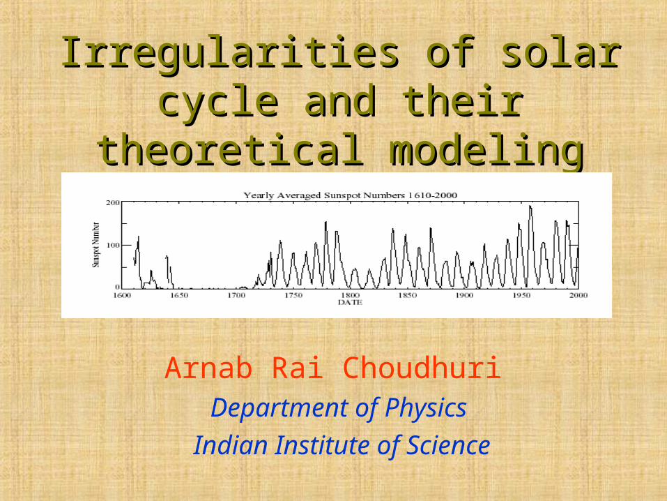
Irregularities of solar cycle and their Irregularities of solar cycle and their theoretical modelingtheoretical modeling

Arnab Rai Choudhuri Department of Physics

Indian Institute of Science

Are there regularities longer than the cycles?

The even-odd or Gnevyshev-Ohl rule (Gnevyshev & Ohl 1948) – The odd cycle was stronger than previous even cycle for cycles10 – 21.

Does the Gleissberg cycle exist?

Difficult to establish or refute at present!

Waldmeier effect (Waldmeier 1935)

WE1 – Anti-correlation between cycle strength and rise timeWE2 – Correlation between cycle strength and rise rate (used to predict strength of a cycle)

Dikpati et al. (2008) claimed that WE1 does not exist in sunspot area data!Karak & Choudhuri (2011) defined rise time as time to grow in strength from 20% to 80%

From Karak & Choudhuri (2011)

WE2 is a stronger effect.WE1 is weaker, but seems to exist!

Choudhuri, Chattejee & Jiang 2007Jiang, Chatterjee & Choudhuri 2007

Correlation between polar field at minimum and next cycle

Are polar faculae good proxies of polar field?From Sheeley (1991)

From Jiang, Chatterjee & Choudhuri (2007)

Hemispheric asymmetry is never very large• Strengths in two hemispheres (max ~20% in last few cycles)•Two hemispheres going out of phase (max ~1 year)•Durations of cycles in two hemispheres

Goel & Choudhuri (2009) – Correlation between asymmetry in polar faculae at sunspot minima and aymmetry in strength of the next cycle

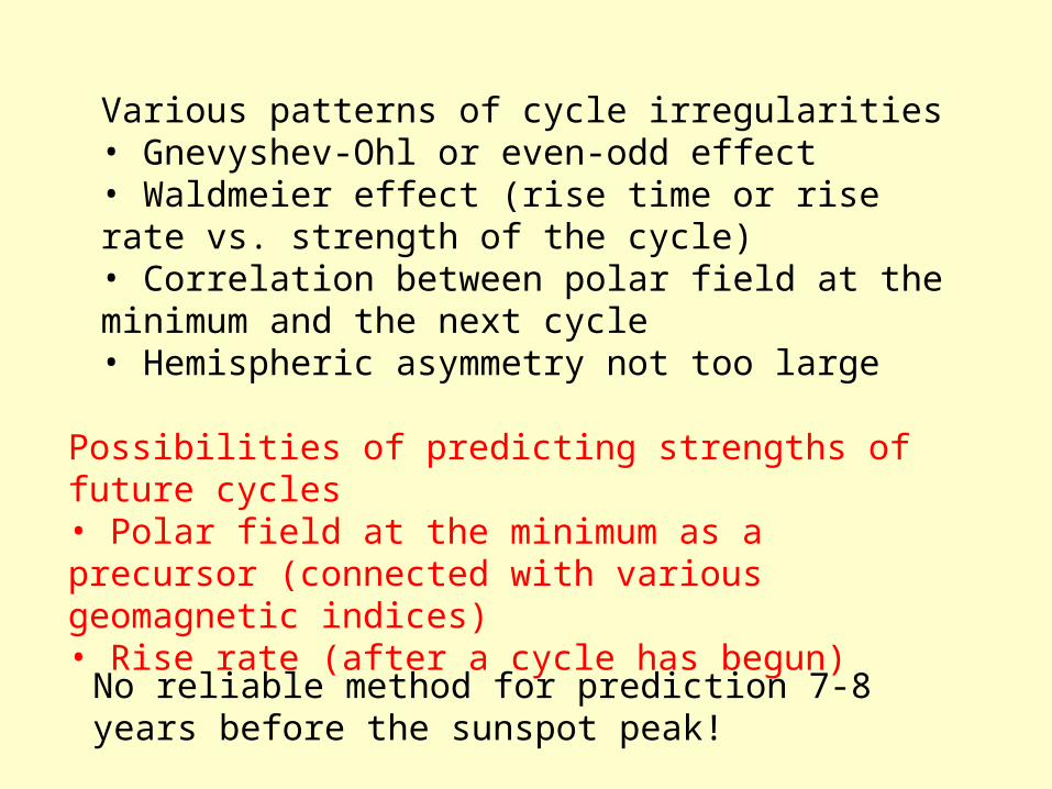
Various patterns of cycle irregularities• Gnevyshev-Ohl or even-odd effect• Waldmeier effect (rise time or rise rate vs. strength of the cycle)• Correlation between polar field at the minimum and the next cycle• Hemispheric asymmetry not too large

Possibilities of predicting strengths of future cycles• Polar field at the minimum as a precursor (connected with various geomagnetic indices)• Rise rate (after a cycle has begun)

No reliable method for prediction 7-8 years before the sunspot peak!

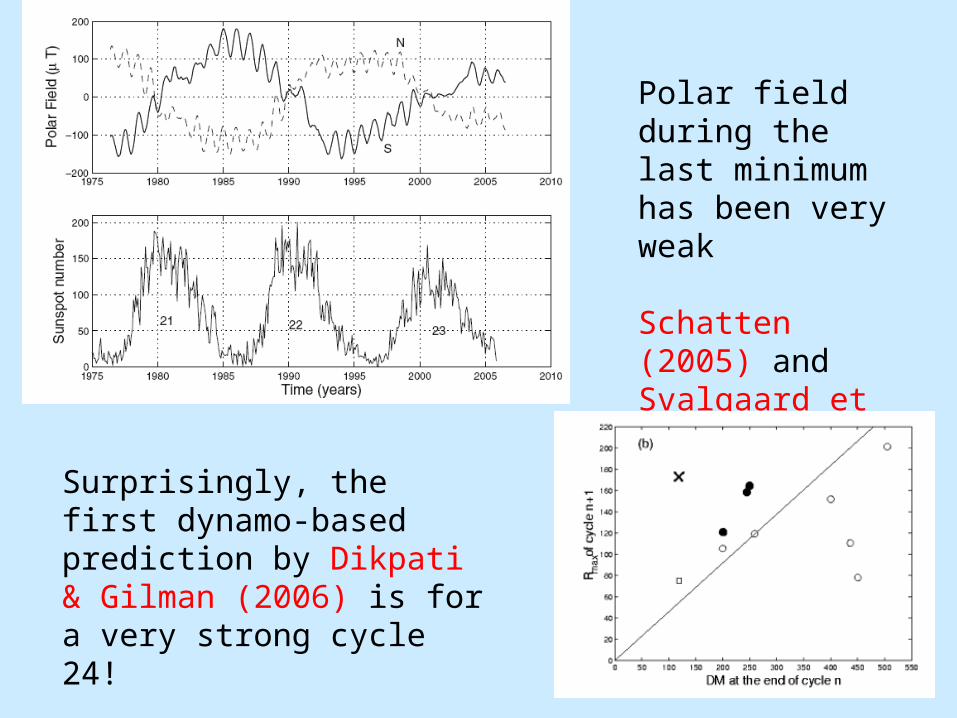
Polar field during the last minimum has been very weak

Schatten (2005) and Svalgaard et al. (2005) predicted a weak cycle 24

Surprisingly, the first dynamo-based prediction by Dikpati & Gilman (2006) is for a very strong cycle 24!

A fun plot from Pesnell (2008)

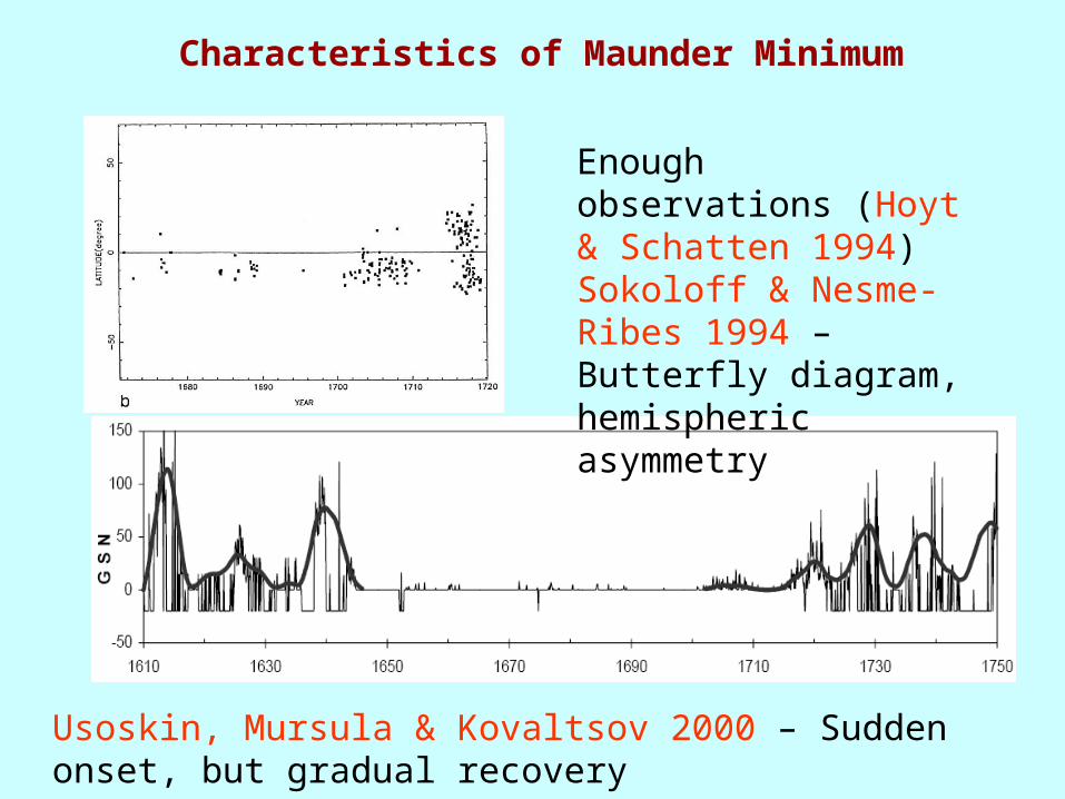
Characteristics of Maunder Minimum

Enough observations (Hoyt & Schatten 1994)Sokoloff & Nesme-Ribes 1994 – Butterfly diagram, hemispheric asymmetry

Usoskin, Mursula & Kovaltsov 2000 – Sudden onset, but gradual recovery

Beer, Tobias & Weiss 1998 – Results from 10Be ice core data, solar wind magnetic field continued to have cycles during Maunder minimumMiyahara et al. 2004 – Similar conclusion from 14C tree ring data,cycles within Maunder minimum were longer

Less solar activity => weaker B in solar wind => more cosmic rays => more production of radio-isotopes 10Be and 14C

History of solar activity before telescopic records reconstructed by Eddy (1977), Stuiver & Braziunas (1989),Voss et al. (1996), Usoskin, Solanki & Kovaltsov (2007)

From Usoskin, Solanki & Kovaltsov (2007) – 27 grand minima and 19 grand maxima in the last 11,000 years!

Are grand minima merely extremes of cycle irregularities?

• Processes which cause cycle irregularities can push the Sun into grand minima• Recovery from grand minima requires B generation processes not involving sunspots

Definitive answer not known!

Our view:

Dynamo generation of magnetic fields

Decay of tilted bipolar sunspots – Babcock 1961; Leighton 1969

Twisting by helical turbulence – Parker 1955; Steenbeck, Krause & Radler 1966

α–effect – works only if B is not very strong

Early solar dynamo models were mostly based on the α-effect

Simulations of flux rise in the rise suggested that B at the bottom of convection zone is 105 G (Choudhuri 1989; D’Silva & Choudhuri 1993; Fan, Fisher & DeLuca 1993) – α-effect would be suppressed

Flux transport dynamo models are primarily based on Babcock-Leighton mechanism

Recovery from grand minima must depend again on the α-effect – spatial distribution or even sign unknown!

Flux transport dynamo in the Sun (Choudhuri, Schussler & Dikpati 1995; Durney 1995)

Differential rotation > toroidal field generation

Babcock-Leighton process > poloidal field generation

Meridional circulation carries toroidal field equatorward & poloidal field poleward

Basic idea was given by Wang, Sheeley & Nash (1991)

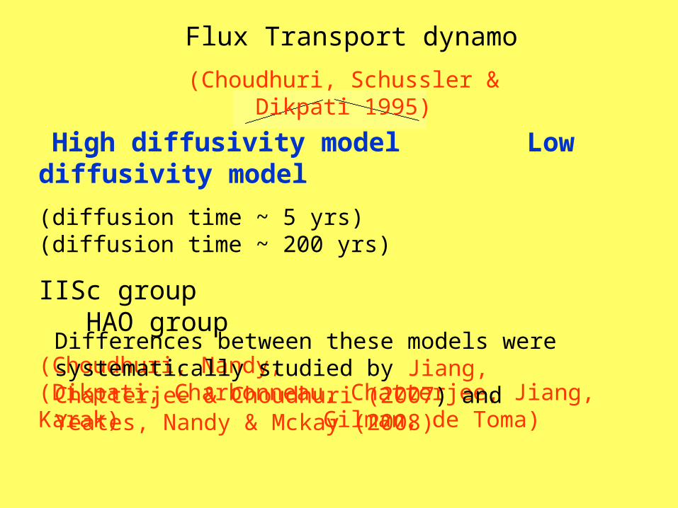
Flux Transport dynamo

(Choudhuri, Schussler & Dikpati 1995)

High diffusivity model Low diffusivity model

(diffusion time ~ 5 yrs) (diffusion time ~ 200 yrs)

IISc group HAO group

(Choudhuri, Nandy, (Dikpati, Charbonneau, Chatterjee, Jiang, Karak) Gilman, de Toma)

Differences between these models were systematically studied by Jiang, Chatterjee & Choudhuri (2007) and Yeates, Nandy & Mckay (2008)

Arguments in favour of high diffusivity model

• Diffusivity of order 1012 cm2/s is what you expect from mixing length theory ~(1/3)vl (Parker 1979)• Helps in establishing bipolar parity (Chatterjee, Nandy & Choudhuri 2004; Hotta & Yokoyama 2010)• Keeps the hemispheric asymmetry small (Chatterjee & Choudhuri 2006; Goel & Choudhuri 2009)• Fluctuations spread all over the convection zone soon, explaining many aspects of observations (Jiang, Chatterjee & Choudhuri 2007)• Behaves properly on introducing fluctuations in meridional circulation (Karak & Choudhuri 2011)

Possible causes of solar cycle irregularities

• Effects of nonlinearities

• Fluctuations in poloidal field generation

• Fluctuations in meridional circulation

Nonlinearity due to back-reaction of B on v

α-quenching:

Long history – Stix 1972; Ivanova & Ruzmaikin 1977; Yoshimura 1978; Schmitt & Schussler 1989

Has a stabilizing effect instead of producing irregularities

Krause & Meinel 1988; Brandenburg et al. 1989 – Nonlinear stability may detemine the mode of the dynamo

Weiss, Cattaneo & Jones (1984) found chaos in some highly truncated models with suppression of differential rotation

Charbonneau, St-Jean & Zacharias (2005), Charbonneau, Beaubien & St-Jean (2007) – The Gnevyshev-Ohl rule may be due to period doubling just beyond bifurcation point

Possible causes of solar cycle irregularities

• Effects of nonlinearities

• Fluctuations in poloidal field generation

• Fluctuations in meridional circulation

What is the source of fluctuations in poloidal field generation?

Joy’s law: Bipolar sunspots have tilts increasing with latitude (D’Silva & Choudhuri 1993)

Their decay produces poloidal field (Babcock 1961; Leighton 1969)

Randomness due to large scatter in tilt angles (caused by convective turbulence – Longcope & Choudhuri 2002)

Mean field equations obtained by averaging over turbulence and there must be fluctuations around themFirst suggested by Choudhuri (1992) and explored by Moss et al. (1992) and Hoyng (1993)Applied to flux transport dynamo by Charbonneau & Dikpati (2000)

Supported by Dasi-Espuig et al. (2010)

Cause of correlation between the polar field at the minimum and the next cycle (Jiang, Chatterjee &

Choudhuri 2007)C – Poloidal field produced here by Babcock-Leighton mechanism

P – Field advected to the pole by meridional circulation

T – Poloidal field diffuses to tachocline to produce next cycle

Correlation arises if C -> T diffusion takes 5-10 years (happens only in high diffusivity model

Prediction of cycle 24 – Dikpati & Gilman (2006) predict a stong cycle from low diffusivity model and Choudhuri, Chatterjee & Jiang (2007) predict a weak cycle from high diffusivity model

A theoretical mean field dynamo model would produce an ‘average’ poloidal field at the end of the cycle.The actual poloidal field may be stronger or weaker!

• The code Surya is run from one minimum to the next minumum in the usual way

• At minimum we change poloidal field above 0.8R to match the observed poloidal field

We adopt the following procedure (Choudhuri, Chatterjee & Jiang 2007)

All calculations are based on our dynamo model (Nandy & Choudhuri 2002; Chatterjee, Nandy & Choudhuri 2004)

Correlations seen in numerical simulations with random kicks at the sunspot minima (from Jiang, Chatterjee & Choudhuri 2007)

High diffusivity

(our model)

Low diffusivity

(Dikpati-Gilman)

Our final results for the last few solar cycles:

(i) Cycles 21-23 are modeled extremely well.

(ii) Cycle 24 is predicted to be a very weak cycle!

From Choudhuri, Chatterjee & Jiang (2007)

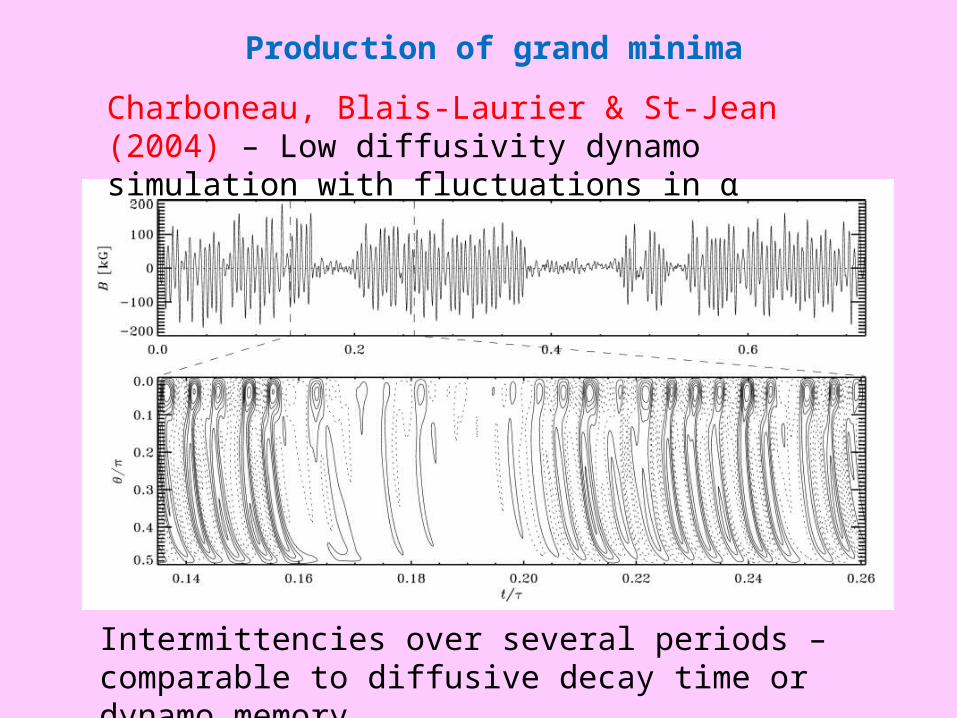
Charboneau, Blais-Laurier & St-Jean (2004) – Low diffusivity dynamo simulation with fluctuations in α

Intermittencies over several periods – comparable to diffusive decay time or dynamo memory

Production of grand minima

Choudhuri & Karak (2009) - Modelling of Maunder minimum with flux transport dynamo

Assumption : Poloidal field drops to 0.0 and 0.4 of its average value in the two hemispheres

From Choudhuri & Karak (2009)

During recovery poloidal field in solar wind shows oscillations, even though there are no sunspots

Choudhuri & Karak (2009) also correctly predicted that we were not entering another grand minimum!!

Possible causes of solar cycle irregularities

• Effects of nonlinearities

• Fluctuations in poloidal field generation

• Fluctuations in meridional circulation

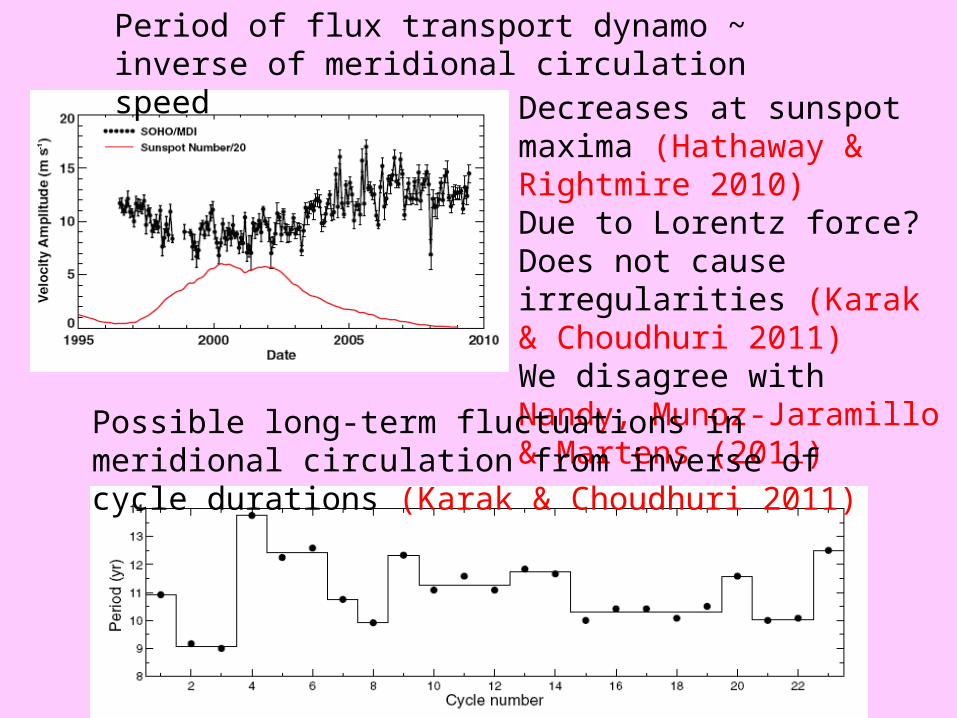
Period of flux transport dynamo ~ inverse of meridional circulation speed

Decreases at sunspot maxima (Hathaway & Rightmire 2010)Due to Lorentz force?Does not cause irregularities (Karak & Choudhuri 2011)We disagree with Nandy, Munoz-Jaramillo & Martens (2011)

Possible long-term fluctuations in meridional circulation from inverse of cycle durations (Karak & Choudhuri 2011)

Suppose meridional circulation slows down

Dynamo period increases

(Yeates, Nandy & Mackay 2008)

Diffusion has more time to act on the fields

Cycles become weaker

Differential rotation generates more toroidal flux

Cycles becomes stronger

Applicable for high diffusivity dynamo

Applicable for low diffusivity dynamo

Explanation of Waldmeier Effect (Karak & Choudhuri 2011)

WE2 is easy to explain!But WE1 is reproduced only in high diffusivity model: weaker meridional circulation causes both longer cycles and weaker cycles.

Karak (2010) matched only the periods of sunspot cycles by varying meridional circulation, but very surprisingly strengths of many cycles also got matched!

Modelling and prediction of actual cycles by using data of polar fields at minima should work properly only when variations of meridional circulation has not been large!!!

Karak (2010) found that a sufficiently large decrease in meridional circulation can cause grand minimum

Periods during grand minimum should be longer!

Various patterns of cycle irregularities• Gnevyshev-Ohl or even-odd effect (explained as nonlinear bifurcation)• Waldmeier effect (caused by fluctuations of meridional circulation in high diffusivity model)• Correlation between polar field at the minimum and the next cycle (caused by fluctuations in poloidal field generation mechanism in high diffusivity model)• Hemispheric asymmetry not too large (due to diffusive coupling between hemispheres)

Conclusions

Grand minima may be caused by• Fluctuations in poloidal field generation• Fluctuations in meridional circulation

Recovery from grand minima cannot be due to Babcock-Leighton mechanism!!