Irreducibility of Polynomials Whose Coefﬁcients are Integersthanga/papers/mnl.pdf ·...

Irreducibility of Polynomials Whose Coefficients are Integers

R. Thangadurai

Harish-Chandra Research Institute

Chhatnag Road, Jhunsi

Allahabad 211019 India

E-mail: [email protected]

Abstract. In this article, we give an account for testing the irreducibility of a given polynomial with integer coefficients over

the field of rational numbers. Apart from the traditional tests like Eisenstein criterion and irreducibility over prime finite field, we

study the recent criteria like those of Ram Murty, Chen et al., Filaseta and so on.

1. Introduction

A polynomial is said to be reducible over a given field if it

is expressible as a product of lower degree polynomials with

coefficients in this field. Otherwise, it is said to be irreducible.

In this article, we shall concentrate on the polynomials

whose coefficients are integers and their irreducibility over the

field of rational numbers (which is denoted by Q). Let Z[X]

be the ring of polynomials with integer coefficients. Let

f (X) = anXn + an−1X

n−1 + · · · + a1X + a0 ∈ Z[X] (1)

of degree n with ai ∈ Z, an �= 0 and the greatest common

divisor (a0, a1, . . . , an) = 1. If f (X) is reducible over Q, then,

by Gauss lemma, we can, as well, assume that the factors of

f (X) also have integer coefficients.

We are interested in the question of deciding whether a given

polynomial is irreducible or not. Consequently, a simple test

or criterion which would give this information is desirable.

Unfortunately, no such criterion which will apply to all the

classes of polynomials has yet been devised; but a number of

tests, or irreducibility criteria have been found so far which

give valuable information for some particular classes of poly-

nomials.

Throughout the article, unless otherwise specified, the irre-

ducibility of f (X) will be over Q.

The most popular irreducibility criterion is due to Eisenstein

[12] which states that:

Criterion # 1. If there exists a prime number p such that p �

an, p|ai for all i = 0, 1, . . . , n − 1 and p2 � a0, then, f (X) is

irreducible over Q.

Such a polynomial f (X) is called Eisenstein polynomial. It

often happens that this criterion is not directly applicable to a

given polynomial f (X), but it may be applicable to f (X + a)

for some constant a. So we try various values of a, hoping to

transform f (X) into a polynomial that satisfies the conditions

of the criterion.

Notice that Eisenstein’s criterion essentially reduces the

problem of factoring a polynomial of degree n to a problem of

factoring n integers, the coefficients of the transformed poly-

nomial, to see if they share a suitable common prime divisor.

Obviously as we try various transformations we will produce

polynomials with larger and larger coefficients, so the compu-

tational task of computing and then checking the factorizations

of those coefficients can be significant.

Moreover, a simple transformation that allows us to apply

Eisenstein’s criterion may not even exist. Indeed, Algebraic

Number Theory predicts for what prime p the above crite-

rion works. In fact, the primes p that make the above criterion

work is really a special type of prime called totally ramified

prime in the finite extension of Q, the field obtained by attach-

ing a root of f (X). This type of primes are rare and hence,

this criterion cannot be applied to test the irreducibility of all

polynomials.

By Probabilistic Galois Theory, it is known that almost all

the polynomials with integer coefficients are irreducible poly-

nomials. Therefore, it is reasonable to look for more such cri-

teria to prove irreducibility of a given polynomial.

However, if we are willing to factor some large integers,

there are other criteria even easier than Eisenstein’s, and these

always work. These criteria, in the literature, are not as popular

Mathematics Newsletter -29- Vol. 17 #2, September 2007

as Eisenstein criterion. The purpose of this article is to give an

exposition of these criteria to test the irreducibility of a given

polynomial with integer coefficients. For older results we refer

to the exposition of Dorwart [9].

2. Preliminaries

We define

u = u(f ) := # {m ∈ Z | f (m) = ±1} .

Clearly, u counts the number of times f is a unit at the integral

arguments.

If f (X) assumes the values ±1 at X = bi for integers bi

(i = 1, 2, . . . , m), then,

f (X) = r(X)

m∏i=1

(X − bi) ± 1 where r(X) ∈ Z[X].

Remark 2.1. (Dorwart and Ore, [10]) If f (X) takes the

value +1 (respectively, −1) at m > 3 distinct integers, then

f (X) cannot take the value −1 (respectively, +1). For, let

b1, b2, . . . , bm be the integers such that f (bi) = 1 for all i.

Then

f (x) = (x − b1)(x − b2) · · · (x − bm)g(x) + 1 (2)

for some g(x) ∈ Z[x]. Suppose that bm+1 is an integer such

that f (bm+1) = −1. Then, from the equation (2), we get

−1 = (bm+1 − b1)(bm+1 − b2) · · · (bm+1 − bm)g(bm+1) + 1

which would imply

(bm+1 − b1)(bm+1 − b2) · · · (bm+1 − bm)g(bm+1) = −2.

Therefore, the differences bm+1 − bi can take the values ±1

and ±2 only. Thus, m ≤ 3.

Remark 2.2. If f (X) is of degree n, then u(f ) ≤ n, whenever

n ≥ 4. For, by Remark 2.1, we see that f (X) cannot take +1

as well as −1 as its value. If f (X) takes the value +1, then it

can take +1 for at most n distinct integers mi’s, as these mi

are the roots of the polynomial f (X) − 1 which is of degree n

again. Hence, u(f ) ≤ n.

When n ≤ 3, f can take values +1 and −1. Hence, we can

take the trivial bound for u(f ) as twice the degree of f ; i.e.,

u(f ) ≤ 2n.

Remark 2.3. If f (X) is of degree n ≥ 8, and it takes values

±1 at m > n/2 distinct integers, then f (X) must be irre-

ducible. By Remark 2.1, it is clear that f (X) can take either

+1 or −1 as its value, but not both. Assume that f (X) takes

the value +1 for m > n/2 > 3 distinct integers. If possible,

suppose that f (X) = g(X)h(X) where g(X) and h(X) are

non-trivial factors of f (X). Since the degree of f is the sum

of the degrees of g and h, it is clear that one of the factors,

say, g will have degree ≥ n/2. Since n/2 > 3, by Remark 2.1,

g cannot take both the values +1 and −1. So, we assume that

g takes the value +1 only. But, whenever f (a) = 1, we have

g(a)h(a) = 1 which implies g(a) = 1 = h(a) and in no way

h(X) can take the value −1, as g cannot take the value −1.

However, since f takes the value 1 for m > n/2 distinct inte-

gers, h(X) also takes the value 1 for m > n/2 distinct integers,

which is a contradiction to that fact that the degree n(h) of h

satisfies n(h) ≤ n/2. Hence, f (X) is irreducible.

Definition 2.1. Brown and Graham [4]) A polynomialg(X) ∈Z[X] is said to be fat if

�(g) := u(g) − n(g) > 0,

where n(g) is the degree of g(X).

Remark 2.4. If f (X) is a fat polynomial, then it is clear that

f has to assume both the values +1 and −1. If not, then +1

(respectively, −1) is assumed by more than the degree of f (X)

distinct number of integers which is not possible. Therefore, by

Remark 2.1, we have n ≤ 3. That is, if f (X) is a fat polynomial,

then its degree is less than or equal to 3.

Remark 2.5. Dorwart and Ore [10] proved that if f (X) is a

fat polynomial of degree n, then f (X) = ±hi(±X+a), where

the polynomials hi(X), i = 1, 2, . . . , 5 are listed below.

h1(X) = X(X − 1)(X − 3) + 1, n = 3, u(f ) = 4.

h2(X) = (X − 1)(X − 2) − 1, n = 2, u(f ) = 4.

h3(X) = 2X(X − 2) + 1, n = 2, u(f ) = 3.

h4(X) = 2X − 1, n = 1, u(f ) = 2.

h5(X) = X − 1, n = 1, u(f ) = 2.

We define

P(f ) := # {n ∈ Z | f (n) = ±p where p is a prime number}to be the number of times f assumes prime values upto units

in Z at the integer arguments. Note that P(f ) = ∞ for many


f (X) ∈ Z[X]. For example, if we consider f (x) = ax + b

with (a, b) = 1, then by Dirichlet’s prime number theorem, it

is known that P(f ) = ∞.

Remark 2.6. (Stackel, 1918, [24]) If P(f ) > 2n, then f (X)

is irreducible. For, suppose f (X) = g(X)h(X) where g, h ∈Z[X] and degrees of g, h > 1. Suppose that p = f (n) =g(n)h(n) is a prime. Then either g(n) or h(n) is ±1. Thus, to

know how many prime values f can assume, it is enough to

know the number of integer solutions to the equation r(x) =±1. Clearly, the equation r(X) = 1 can have at most n(r)

distinct integer solutions. Therefore r(X) = ±1 can have at

most twice of the degree of r(X) distinct integer solutions.

Thus, by noting that the sum of the degrees of g and h is n, we

have, P(f ) ≤ 2n, which is a contradiction.

For example, suppose that f (X) = 3X2 + 11X + 121 ∈Z[X]. It turns out that f (X) is not an Eisenstein polyno-

mial. Note that f (−7) = 191, f (−6) = 163, f (−1) =113, f (3) = 181 and f (5) = 251. Since 113, 163, 181, 191

and 251 are all prime numbers, by Remark 2.6, we conclude

that f (X) is irreducible over Q.

Remark 2.7. (References [18] and [19]) Note that

Remark 2.6 can be improved under some additional assump-

tions. Indeed, in Remark 2.6, it suffices to conclude that

if we can find n + 1 integers m1, m2, . . . , mn+1 such that

|mi − mj | > 2 and f (mi) is a prime or a unit, then f (X)

has to be irreducible. This is because of the following obser-

vation. Suppose f (X) = g(X)h(X). Therefore, g(mi) = ±1

or h(mi) = ±1. Using the given condition, first we claim

that g(X) = ±1 (respectively, h(X) = ±1) can have at most

d = n(g) (respectively, n(h)), degree of g, solutions in Z. For,

if g(X) = bdXd + bd−1X

d−1 + · · · + b0 and g(m1) = 1 and

g(m2) = −1, then we have

bd(md1 − md

2) + bd−1(md−11 − md−1

2 )

+ · · · + b1(m1 − m2) = 2.

This implies that (m1 − m2) divides 2 - a contradiction to the

fact that |mi − mj | > 2. Hence g(X) = ±1 (respectively,

h(X) = ±1) can have at most n(g) (respectively, n(h)) solu-

tions. Therefore, the solutions of g(X) = ±1 and h(X) = ±1

together will not exceed the value n(g) + n(h) = n. Hence, if

f (X) assumes more than n+ 1 prime values or unit, it cannot

be reducible, because of the above reason.

For example, consider the polynomial f (X) = X6 −3X5 −87X4 + 118X3 − 33X2 + 21X − 1. In this case, we can easily

compute the values

f (−22) = 107187629,

f (−8) = −58601,

f (−4) = −23269,

f (0) = −1,

f (12) = 634859,

f (18) = 19888469,

f (30) = 588786929.

Each of the arguments −22, −8, . . . , 30 differs by more than

2 from the others, and each of the 7 values of f (k) is a prime

or a unit, so it follows that f (x) is irreducible over the integers

(and therefore over the rationals).

Remark 2.8. (J. Brillhart, 1980, [12]) If f (X) assumes a

prime value for a sufficiently large integer, then f (X) is irre-

ducible. For, suppose f (X) is reducible and hence f (X) =g(X)h(X), where g, h ∈ Z[X]. Let {bi} and {b′

j } be all the

integer roots of the polynomials g(X) ± 1 and h(X) ± 1

respectively. Define M1 = maxi |bi | and M2 = maxj |b′j |. Let

M := max{M1, M2}. We can take this M to be the desired

large integer. Since f (m) is a prime for an integer m with

|m| > M, then, clearly, either g(m) or h(m) is ±1 which

is impossible, from the definition of M. Therefore, f (X) is

irreducible.

In particular, if P(f ) = ∞, then, f (X) must be irreducible.

The converse, unfortunately, is not true. That is, if f (X) is

irreducible, we cannot expect, in general, that P(f ) = ∞. In

fact, we give an example of an irreducible polynomial f with

P(f ) = 0 of any degree n > 1. If we take

f (X) = Xn + 105X + 12,

then, it is irreducible by Eisenstein criterion. However, we have

P(f ) = 0. For, since f (X) = X(Xn−1 + 105) + 12, for any

integer value m, we have, f (m) is even. Hence, if at all it can

produce primes p, then the only possibility is p = 2. However,

if we consider

g±(X) = f (X) ± 2

then, g±(X) is irreducible by Eisenstein criterion and hence,

P(f ) = 0.


In the above counter example, we had 2 as a common divisor

of f (m) for every m ∈ Z. Hence, it is reasonable to have the

following definition.

Definition 2.2. Let f (X) ∈ Z[X]. The fixed divisor of f ,

denoted by df , is the largest integer d such that d|f (n) for all

n ∈ Z.

For example, if f (X) = X2 + 9X − 4, then df = 2.

Conjecture 1. (Bunyakovsky, [5]) If f (X) ∈ Z[X] is irre-

ducible, then P(g) = ∞ where g(X) = d−1f f (X).

The only case, for which Conjecture 1 is known to be true,

is f (X) = aX + b by Dirichlet Prime Number Theorem (See

for instance, [1]). Otherwise, Conjecture 1 remains completely

unsolved.

We define the following ‘heights’ of f (X);

H1 = max0≤i≤n−1

∣∣∣∣ ai

an

∣∣∣∣and

H2 = max0≤i≤n−1

∣∣∣∣ ai

an

∣∣∣∣1/(n−i)

.

If one has bounds for the roots of f (X) in the complex

plane, then we can prove some irreducibility criteria using

these bounds. Hence, first, we give some bounds for any com-

plex root of f (X) in the following three lemmas.

Lemma 2.1.1. Let f (X) be a polynomial as defined in (1).

Suppose an−k = 0 for all k = 1, 2, . . . , r where 0 ≤ r ≤ n−1.

If α ∈ C is a root of f (X), then

|α| < H1/(r+1)

1 + 1.

Remark 2.9. If r = 0 in the statement of Lemma 2.1.1, then,

we have an−1 �= 0. This case was proved by Cauchy [6], Brill-

hart [2] and Ram Murty [23].

Proof. Let α ∈ C be a root of f (X). Since α is a root of f (X)

and an−k = 0 for all k = 1, 2, . . . , r, we have

−anαn = an−r−1α

n−r−1 + · · · + a1α + a0.

�⇒ −αn = an−r−1

an

αn−r−1 + · · · + a1

an

α + a0

an

.

Therefore,

|α|n ≤ H1(|α|n−r−1 + · · · + |α| + 1) = H1

( |α|n−r − 1

|α| − 1

).

(3)

If |α| ≤ 1, then clearly, |α| < H1

r+1

1 +1 as H1 > 0. If |α| > 1,

then by (3), we have,

|α|n(|α| − 1) ≤ H1(|α|n−r − 1) < H1|α|n−r

�⇒ |α|r (|α| − 1) < H1.

Since

(|α| − 1)r+1 ≤ |α|r (|α| − 1),

we have,

(|α| − 1)r+1 < H1

and hence we get |α| < H1/(r+1)

1 + 1. •

Lemma 2.1.2. ([21], Page 53, Lemma 4) Let f (X) be a poly-

nomial as defined in (1). If α ∈ C is a root of f (X), then

|α| < 2H2.

Proof. Set bi = ai/an for all i = 0, 1, 2, . . . , n − 1. Let

c := max0≤i≤n−1

{|bi |1/(n−i)}

and η = α

c.

To prove the lemma, it is enough to prove |η| < 2, as c = H2.

By definition, we have, |ai/an| ≤ cn−i for all i =0, 1, 2, . . . , n − 1. Then we have,

an

(ηn + bn−1

cηn−1 + · · · + b0

cn

)

= an

(1

cnαn + bn−1

cnαn−1 + · · · + b0

cn

)

= 1

cn(anα

n + an−1αn−1 + · · · + a0)

= 1

cnf (α) = 0.

Since an �= 0, we have,

ηn + bn−1

cηn−1 + · · · + b0

cn= 0.

Since |bi | ≤ cn−i , we get,

|η|n ≤ 1 + |η| + |η|2 + · · · + |η|n−1. (4)

If |η| ≥ 2, then by above inequality (4) we have

|η|n ≤ |η|n − 1

|η| − 1<

|η|n|η| − 1

which implies |η| < 2, a contradiction. Hence |η| < 2. That

is, |α| < 2c. Since c = H2, we get the result. •


Lemma 2.1.3. (Ram Murty, [23]) Let f (X) be a polynomial

as defined in (1). Assume that an ≥ 1, an−1 ≥ 0 and |ai | ≤ M

for i = 0, 1, . . . , n − 2 and for some M > 0. If α ∈ C is a

root of f (X), then α satisfies either

(α) ≤ 0 or |α| <1 + √

1 + 4M

2,

where (z) means real part of z ∈ C.

Proof. If an−1 = 0, then, by Lemma 2.1.1, we have |α| <√H1 + 1 where H1 ≤ M/an. Hence, it is an easy verification

that, in this case, we get,

|α| <√

H1 + 1 ≤ 1 + √1 + 4M

2.

Thus, we can assume that an−1 ≥ 1.

Let z ∈ C such that |z| > 1 and (z) > 0. Then first we

claim that∣∣∣∣f (z)

zn

∣∣∣∣ > 0 whenever |z| ≥ 1 + √1 + 4M

2.

For,∣∣∣∣f (z)

zn

∣∣∣∣ =∣∣∣∣an + an−1

z+ · · · + a1

zn−1+ a0

zn

∣∣∣∣≥∣∣∣∣an + an−1

z

∣∣∣∣−( |an−2|

|z|2 + · · · + |a0||z|n

)

≥ (

an + an−1

z

)− M

(1

|z|2 + · · · + 1

|z|n)

> 1 − M

|z|2 − |z| = |z|2 − |z| − M

|z|2 − |z| ,

as an, an−1 ≥ 1 and (z) > 0. Hence,∣∣∣∣f (z)

zn

∣∣∣∣ > 0 whenever|z|2 − |z| − M

|z|2 − |z| ≥ 0.

But, whenever |z| ≥ 1 + √1 + 4M

2, we have

|z|2 − |z| − M

|z|2 − |z|≥ 0. Thus we conclude that

∣∣∣∣f (z)

zn

∣∣∣∣ > 0 whenever |z| ≥ 1 + √1 + 4M

2

which proves our claim.

To end the proof of the lemma, we assume that (α) > 0.

Therefore, we have to prove

|α| <1 + √

1 + 4M

2.

Also, α �= 0 as (α) > 0. If |α| < 1, then there is nothing to

prove, as M ≥ 0 and1 + √

1 + 4M

2≥ 1.

Suppose |α| ≥ 1 + √1 + 4M

2. Therefore, by the above

claim, we get|f (α)||α|n > 0, which is a contradiction to the fact

that f (α) = 0, as α is a root of f (X). Hence, we get the

result. •

3. Irreducibility Criteria

Criterion # 2. It is an easy observation that if f (X) is

reducible in Z[X], then it is reducible over Fp[X], where Fp

is the finite field of p elements. Hence, we have the following

criterion.

If f (X) is irreducible over Fp[X] for some prime number

p, then f (X) is irreducible over Q.

Converse is not true. That is, if f (X) is irreducible over Q,

then it is not necessarily irreducible over Fp for some prime

number p.

For example, if f (X) = X4 + 1, then it is irreducible over

Q, by Eisenstein criterion. But, it is reducible over Fp for every

prime number p. When p = 2, clearly, f (X) = X4 + 1 ≡(X2+1)2 (mod 2) and hence it is reducible over F2. Let p ≥ 3

be any prime. Then, p satisfies, p2 ≡ 1 (mod 8). That is,

8|(p2 − 1) and hence

(X8 − 1)|(Xp2−1 − 1) �⇒ X(X4 + 1)(X4 − 1)|(Xp2 − X).

That is, f (X) is a factor of the polynomial Xp2 − X. The

splitting field K of the polynomial Xp2 − X over Fp is Fp2 .

Clearly, [K : Fp] = 2.

If f (X) is irreducible over Fp for some prime p ≥ 3, then

K1 = Fp(α), where α is a root of f (X), is an non-trivial field

extension of Fp of dimension 4. Also, since f (X) is a factor

of Xp2 − X, K1 is an intermediate field of K over Fp. Hence,

we have,

[K1 : Fp]|[K : Fp] �⇒ 4|2,

which is absurd. Hence f (X) is reducible over Fp for all

primes p.

More generally, Driver, Leonard and Williams [11] gave a

necessary and sufficient condition for an 4th degree polyno-

mial with integer coefficients which is irreducible over Q; but

reducible over Fp for every prime number p. Also, another


recent result of Guralnick, Schacher and Sonn, [17] states that

for any composite integer n ≥ 4, there exists an irreducible

polynomial f (X) ∈ Z[X] of degree n which is reducible over

Fp for every prime p.

Now, we give a criterion involving P(f ). More precisely,

we have the following criterion which was proved by Ore [22].

Criterion # 3. If P(f ) ≥ n+3 where n is the degree of f (X),

then f (X) is irreducible over Q.

Since the original proof is not easily available, we present

the proof here for all polynomials of degree ≥ 7 for simplicity.

Proposition 3.1. If P(f ) + 2u ≥ n + 4, then f (X) is irre-

ducible.

Proof. If possible, we assume that f (X) = g(X)h(X) where

g, h ∈ Z[X] and degrees of g (say n(g)) and h (say n(h)) are

≥ 1. Without loss of generality we may assume that �(g) ≥�(h).

Claim. �(g) + �(h) ≥ P(f ) + 2u − n. (5)

For each m ∈ Z such that f (m) is a prime number, we have

either g(m) or h(m) must be a unit. While for each m ∈ Z

such that f (m) is a unit, we have g(m) and h(m) is a unit.

Therefore, u(g) + u(h) ≥ P(f ) + 2u. Therefore, we have

�(g) + �(h) = u(g) − n(g) + u(h) − n(h) = u(g)

+ u(h) − n ≥ P(f ) + 2u − n

as claimed.

Since by assumption P(f )+ 2u ≥ n+ 4, we have P(f )+2u−n ≥ 4. Therefore, by the claim, we get, �(g)+ �(h) ≥ 4.

If �(g) > 0 and �(h) > 0, then by the definition, we have

g and h are fat polynomials. Hence by Remark 2.4, we have

n(g), n(h) ≤ 3 which is not possible as its sum is ≥ 7. There-

fore, only g(X) is fat. Since h(X) is not fat and n ≥ 7, we

have n(h) ≥ 4 and �(h) ≤ 0. Also, since �(g) + �(h) ≥ 4,

we have �(g) = u(g) − n(g) ≥ 4 which would imply u(g) ≥4 + n(g), which is not possible because n(g) ≤ 3 and u(g) ≤2n(g). Thus this contradiction shows that f (X) has to be

irreducible. •Corollary 3.1. If P(f ) ≥ n + 2 and u ≥ 1, then f (X) is

irreducible.

Proof of criterion # 3. If P(f ) ≥ n+4, then by Proposition 3.1,

clearly, f (X) is irreducible. So, it is enough to assume that

P(f ) = n + 3.

Suppose we assume that f (X) = g(X)h(X) where g, h ∈Z[X] of positive degree. By (5) and P(f ) = n + 3, it is clear

that either �(g) or �(h) is positive. Since the degree of f is ≥ 7,

it is clear that exactly one of the factors must be fat. Hence,

either g or h coming from the list stated in Remark 2.5; but

not both.

Without loss of generality, we may assume that g is fat and

h is not fat. Therefore, �(g) ≥ 1 and �(h) ≤ 0 and hence

�(g) + �(h) ≤ �(g). However, by (5), we know that �(g) +�(h) ≥ P(f ) + 2u − n ≥ n + 3 − n = 3. Thus, we arrive

at �(g) ≥ 3, which would implies u(g) ≥ n + 3. Since g is

coming from the list stated in Remark 2.5, we conclude that

u(g) = n+1, which is a contradiction to u(g) ≥ n+3. Hence

f (X) is irreducible. •The following Conjecture (which is still open) says that the

criterion # 3 is tight.

Conjecture 2. (Chen, et al. [8]) For each n ≥ 2, there does

exist a polynomial f (X) ∈ Z[X] which is reducible and

P(f ) = n + 2.

When n = 2, take f (X) = X(X−4) which has P(f ) = 4.

When n = 3, consider f (X) = (X−5)(1+X(X−3)) which

has P(f ) = 5.

Define

P +(f ) = # {n ∈ Z / f (n) > 0 is prime} .

Clearly P +(f ) counts the number of positive prime values

that f assumes at distinct integral arguments. Recently Chen

et al. [8] proved the following theorem.

The following Theorem gives another criterion for irre-

ducibility which is similar to Criterion # 3.

Theorem 3.2. (Chen, et al. [8]) If f (X) is reducible, then

P +(f ) ≤ n. On the other hand, there is a reducible polynomial

f ∈ Z[X] for which P +(f ) = n.

Criterion # 4. If we can find an integer m which is bigger

than the ‘height’ of the given polynomial f (X) and f (m) is

prime, then f (X) is irreducible.

Since f (X) is a given polynomial, we know its coeffi-

cients and therefore we can compute H1 and H2 as defined

in section 2. Also, we can able to compute r as defined in

Lemma 2.1.1. Put

H = min{H

1/(r+1)

1 + 1, 2H2}.


Theorem 4.1. If f (X) is a polynomial as defined in (1) and if

there exists an integer m ≥ H + 1 such that f (m) is a prime

number, then, f (X) is irreducible.

Proof. Let f (X) be defined as in (1). Let α ∈ C be a root of

f (X). By Lemmas 2.1.1 and Lemma 2.1.2, we have

|α| < H1/(r+1)

1 + 1 and |α| < 2H2.

Hence we get

|α| < H.

Suppose f (X) is reducible, say f (X) = g(X)h(X) where

g(X) and h(X) in Z[X] are of positive degree. Since f (m) is

a prime for some integer m ≥ H + 1, we have either g(m) or

h(m) is ±1. Without loss of generality, we may assume that

g(m) = ±1. Write, g(X) = c∏

i (X−αi) where αi ∈ C roots

of g(X) and c is the leading coefficient of g. Since αi are the

roots of f , we have |αi | < H. Therefore,

1 = |g(m)| = |c|∏

i

|m − αi |

≥∏

i

(m − |αi |) >∏

i

(m − H) ≥ 1,

a contradiction. Hence f (X) must be irreducible. •Remark 4.2. Theorem 4.1 with r = 0 is the best possible

in the following sense. Consider the reducible polynomial

f (X) = (X−9)(X2 +1) = X3 −9X2 +X−9 having H1 = 9

and hence H = H1 + 1 = 10. Though f (10) = 101 a prime,

it is a reducible polynomial.

Remark 4.3. (Reference, [18]) By assuming the truth of the

Conjecture 1, it is always possible to use Theorem 4.1 to proof

the irreducibility of f (X). On the other hand, it won’t always

be easy. For example, the first prime value of the polynomial

f (X) = X12 + 488669 occurs with X = 616980 and has

70 decimal digits.

Corollary 4.1. Let p be any prime number and b ≥ 6 be any

integer. Suppose p is written in base b as follows:

p = anbn + an−1b

n−1 + · · · + a1b + a0;ai ∈ {0, 1, 2, . . . , b − 1}, an �= 0 and an−1 ∈ {0, 1}.

Then the polynomial f (X) = anXn+an−1X

n−1 +· · ·+a1X+a0 is irreducible.

Proof. Assume that an−1 = 0. Then, clearly, H1 ≤ b − 1 and

r = 1. Therefore, H ≤ 1 + √b − 1. If we can prove that

b > H+1, then, sincef (b) is a prime number, by Theorem 4.1,

we can conclude that f (X) is irreducible. So, it is enough to

show that b > 2 + √b − 1 for all b ≥ 3. Indeed, a trivial

calculation reveals this fact and hence the result.

Now, assume that an−1 = 1. Therefore, H2 ≤ √b − 1 and

hence, H ≤ 2√

b − 1. So, it is enough to prove, b − 1 >

2√

b − 1 for all b ≥ 6, which is true. Hence, by Theorem 4.1,

f (X) is irreducible. •The prime number 104729 = 105 +4×103 +7×102 +2×

10+9 in usual decimal system. Consider the digit polynomial

f (X) = X5 + 4X3 + 7X2 + 2X + 9. Clearly, H1 = 9 and

r = 1. Therefore, we have 10 >√

H1 + 2 = 3 + 2 = 5 such

that f (10) is a prime. By Theorem 4.1, we see that f (X) is

irreducible. In fact, the following more general result is true.

Theorem 4.2. (Brillhart, Filaseta and Odlyzko, [3] and Ram

Murty, [23]) Let b ≥ 2 and p be a prime written in base b

p = anbn + an−1b

n−1 + · · · + a1b + a0.

Then the digit polynomial f (X) defined in (1) is irreducible.

The case when b = 10, Theorem 4.2 was proved by

Cohen (see [3]). We prove the above theorem for all b ≥ 3

using Lemma 2.1.3. The case b = 2 is slightly technical and

we leave the proof here.

Proof. Suppose the digit polynomial f (X) = g(X)h(X) with

g(X) and h(X) are non-constant polynomials in Z[X]. Since

f (b) is prime, we have either g(b) or h(b) is ±1. Without

loss of generality, we may assume that g(b) = ±1. Write,

g(X) = c∏

i (X − αi) where αi ∈ C roots of g(X) and c

is the leading coefficient of g. Since αi are the roots of f ,

and 0 ≤ ai ≤ b − 1, we have M = b − 1 in Lemma 2.1.3.

Therefore, either (αi) ≤ 0 or

|αi | <1 + √

1 + 4(b − 1)

2.

So,

1 = |g(b)| ≥∏

i

|b − αi |.

Note that αi �= 0. If (αi) ≤ 0, then |b − αi | > b. If

|αi | <1 + √

1 + 4(b − 1)

2, then |αi | < b − 1 and hence

(b − |αi |) > 1. Hence in both the cases, we have |b −αi | > 1.

Hence, we get,

1 = |g(b)| > 1

which is absurd and hence f (X) is irreducible. •


Other criteria. Here we state the other known criteria which

work for special types of polynomials.

Theorem 5.1. (Filaseta, [14]) Let f (X) be a polynomial

defined as in (1). Assume that ai ≥ 0 and b > 1 is an integer

such that f (b) is a prime number. Let N1 = π/ sin−1(1/b)

and N2 = π/ tan−1(1/b).

(i) If n < N1, then f (X) is irreducible.

(ii) There exists a polynomial g(X) ∈ Z[X] of degree m ≥ N2

such that g(X) is reducible and g(b) is a prime number.

Theorem 5.2. (Filaseta, [14]) Let f (X) be a polynomial

defined as in (1). Suppose 0 ≤ ai ≤ an1030. If f (10) is a

prime, then f is irreducible.

Note that Theorem 5.1 will imply that for a polynomial f (x)

with non-negative coefficients of degree ≤ 31, if it happens

that f (10) is a prime, then f (x) is irreducible. To show the

sharpness of the theorem, Filaseta [14] gives the following

example. He considers the reducible polynomial

g(X) = X32 + 130X2

+ 5603286754010141567161572637720X

+ 61091041047613095559860106059529,

of degree 32 and having non-negative integer coef-

ficients. It is an easy computation that g(10) =217123908587714511231475832449729 is a prime number.

This also shows that the upper bound 1030 on the coefficients

in Theorem 5.2 is rather sharp.

Further, one can compute g(11) and g(12) and con-

clude that they are composite numbers. Since H1 =61091041047613095559860106059529 and H

1/311 = 10.6,

by Theorem 4.1, it is clear that g(m) is composite for all

m ≥ 13.

Theorem 5.3. (Filaseta, [13]) Let b > 2 be an integer and

1 ≤ w < b be any integer. Let p be any prime such that

wp = anbn + an−1b

n−1 + · · · a1b + a0;0 ≤ ai ≤ b − 1, an �= 0.

Then the polynomial f (X) = anXn+an−1X

n−1 +· · ·+a1X+a0 is irreducible.

Remark 5.1. Theorem 5.3 is further improved when b = 10

by Filaseta [14] as follows. Let f (X) be a polynomial as

defined in (1) together with 0 ≤ ai ≤ 5.79 × 107. If f (10) =wp for some w ∈ {1, 2, . . . , 9} and for some prime p, then f

is irreducible.

Similar to Theorem 5.3, we can improve Theorem 4.1 as

follows.

Theorem 5.4. (K. Girstmair, [16]) Let f (X) be the polyno-

mial as in (1) and let H be defined as in Theorem 4.1. If d and

m are positive integers such that m ≥ H + d and

f (m) = ±d · p

for some prime number p not dividing d, then f (X) is irre-

ducible.

Proof. One can prove this fact as we have proved Theorem 4.1.

We shall omit the proof here. •In [20], Lipka proved that if f (X) is a polynomial as defined

in (1) and a0 = b0pk where b0 �= 0 and p is a large enough

prime, then f (X) is irreducible over Q.

More recently, Finch and Jones [15], have characterized

irreducible polynomials of 4th degree having coefficients from

the set {−1, 0, 1}. Also, Chahal and Ram Murty [7] studied

the converse of Conjecture 1 in the number field set-up. More

precisely, suppose that K is a finite extension of Q. Let OK be

its ring of integers. Then they proved the following theorem:

Theorem 5.5. (Chahal and Ram Murty, [7]) Suppose that

f (X) ∈ OK [X] is a polynomial with coefficients from OK

with non-zero discriminant. If f (X) represents an irreducible

element of OK infinitely often, then either f (X) is an irre-

ducible polynomial or f (X) = g(X)h(X), where h(X) is an

irreducible polynomial and g(X) is a linear factor.

Acknowledgment: I am thankful to Prof. N. Raghavendra for

the reference [21] for Lemma 2.1.2.

References

[1] Tom M. Apostol, Introduction to Analytic Number The-

ory, Springer-Verlag, (1976).

[2] J. Brillhart, Note on Irreducibility Testing, Math. of

Computation, 35 (1980) No. 152, 1379–1381.

[3] J. Brillhart, M. Filaseta and A. Odlyzko, On an irre-

ducibility theorem of A. Cohen, Canad. J. Math., 33

(1981), No. 5, 1055–1059.


[4] W. S. Brown and R. L. Graham, An irreducibility cri-

terion for polynomials over the integers, Amer. Math.

Monthly, 76 (1969), 795–797.

[5] V. Bunyakovsky, Sur les diviseurs numeriques invari-

ables des fonctions rationelles entieres, Mem. Acad. Sci.

St. Petersberg, 6 (1857) 305–329.

[6] A. L. Cauchy, Exercises de mathematiques, J. Ecole

Poly., 25 (1837), 176.

[7] J. S. Chahal and M. Ram Murty, Irreducible polynomi-

als over number fields, The Riemann zeta function and

related themes, 39–43, Ramanujan Math. Soc. Lect.

Notes Ser., 2, Ramanujan Math. Soc., Mysore, 2007.

[8] Y. G. Chen, G. Kun, G. Pete, I. Z. Ruzsa and A. Timar,

Prime values of reducible polynomials, II, Acta Arith.,

104.2 (2002), 117–127.

[9] H. L. Dorwart, Irreducibility of Polynomials, Amer.

Math. Monthly, 42 (1935), No. 6, 369–381.

[10] H. L. Dorwart and O. Ore, Criteria for the irreducibil-

ity of polynomials, Annals of Math. 34 (1933), No. 1,

81–94.

[11] E. Driver, P. A. Leonard and K. S. Williams, Irre-

ducible quartic polynomials with factorizations mod-

ulo p, Amer. Math. Monthly, 112 (2005), No. 10,

876–890.

[12] F. G. M. Eisenstein, Uber die Irreductibilitat und einige

andere Eigenschaften der Gleichung, von welcher die

Theilung der ganzen Lemniscate abhangt, J. reine

angew. Math., 39, (1850), 166–167.

[13] M. Filaseta, A further generalization of an irreducibil-

ity theorem of A. Cohn, Canad. J. Math., 34 (1982),

1390–1395.

A Classical Proof of the Fundamental Theoremof Algebra Dissected

R. B. BurckelDepartment of Mathematics

Kansas State UniversityManhattan, Kansas 66506, U.S.A

As is well-known, there is a plethora of proofs of the

Fundamental Theorem of Algebra (FTA) within classical

function theory. Elegant as they are, they often intimidate the

[14] M. Filaseta, Irreducibility criteria for polynomials

with non-negative coefficients, Canad. J. Math., 40

(1988), No. 2, 339–351.

[15] C. Finch and L. Jones, On the irreducibility of

{−1, 0, 1}-quadrinomials, Integers, 6 (2006), # A 16.

[16] K. Girstmair, On an irreducibility criterion of M. Ram

Murty, Amer. Math. Monthly, 112 (2005), No. 3,

269–270.

[17] R. Guralnick, M. Schacher, J. Sonn, Irreducible poly-

nomials which are locally reducible everywhere, Proc.

Amer. Math. Soc., 133 (2005), No. 11, 3171–3177.

[18] http://www.mathpages.com/home/kmath406.htm

[19] B. Kirkels, Irreducibility certificates for polynomials

with integer coefficients, M. Sc Thesis, Radboud Uni-

versiteit Nijmegen, The Netherlands, (2004). URL

address:

http://www.math.ru.nl/∼bosma/students/kirkels/mscthesis.pdf

[20] S. Lipka, Uber die Irreduzibilitat von Polynomen,

Math. Ann., 118 (1941) 235–245.

[21] M. S. Narasimhan, R. R. Simha, R. Narasimhan and

C. S. Seshadri, Riemann surfaces, Mathematical Pam-

phlets, 1, Tata Institute of Fundamental Research,

Bombay, (1963).

[22] O. Ore, Einige Bemerkungen uber Irreduzibilitat,

Jahresber. Deutsch. Math.-Verein., 44 (1934),

147–151.

[23] M. Ram Murty, Prime numbers and irreducible poly-

nomials, Amer. Math. Monthly, 109 (2002), No. 5,

452–458.

[24] P. Stackel, Arithmetische Eigenschaften ganzer Funk-

tionen, J. reine angew. Math., 148 (1918), 101–112.

undergraduate teacher who feels that his students lack

the necessary background. But one of these proofs, when

stripped to its essentials (which this note aims to do), is


fully accessible to second-semester calculus students. It uses

only

(1) the trivial fact that a polynomial is asymptotic to its lead

term,

(2) the relation between D1f (x + iy) and D2f (x + iy)for a

complex-differentiable function f

[that is, the Cauchy-Riemann equation D2 = iD1], and

(3) Fubini’s theorem on inverting the order of integrations of

a continuous function on a rectangle.

Here is how it goes:

Suppose that p(z) is a monic polynomial of degree n ≥ 1

having coefficients in C, the complex numbers, but having no

zero in C. Then P(z) := p(z)p(z) is one of degree 2n, which

moreover is positive at every real number. For appropriately

large positive integer N we have

1

|P(z)| <2

|z|2n∀z ∈ C with |z| ≥ N. (1)

The five magic numbers for the sequel (whose post facto gen-

esis the reader will immediately perceive at the end) are

A :=∫ 1

−1

1

P(x)dx, a positive real number, (2)

Y :=(

4π

A

) 12n−1

+ N, (3)

X :=(

8Y

A

) 12n

+ N, (4)

B :=∫ X

−X

1

P(x)dx > A, since X > 1 and

P(x) > 0 for all real x, (5)

C :=∫ X

−X

1

P(x + iY )dx. (6)

Since Y > N , from (1) we get

|C| ≤ 2

Y 2n

∫ X

−X

1

[(x/Y )2 + 1]ndx ≤ 2

Y 2n

∫ X

−X

1

(x/Y )2 + 1

dx = 4

Y 2n−1tan−1(X/Y ) <

4

Y 2n−1

π

2

(3)<

A

2. (7)

Next note that

C − B =∫ X

−X

[1

P(x + iY )− 1

P(x)

]

dx =∫ X

−X

∫ Y

0D2

[1

P(x + iy)

]dy dx

=∫ X

−X

∫ Y

0iD1

[1

P(x + iy)

]dy dx

by

Cauchy-Riemann

=∫ Y

0i

[1

P(X + iy)− 1

P(−X + iy)

]dy, by Fubini.

Since X > N , it follows from this equality and (1) that

|C − B| ≤∫ Y

0

4

(X2 + y2)ndy <

4

X2nY

(4)<

A

2. (8)

From (7) and (8) follows |B| < A, contrary to (5). Hence no

such polynomial p exists.

If students know about Leibniz’ rule for differentiating

under the integral sign (an easy consequence of Fubini, to be

sure) and are comfortable with the complex exponential func-

tion, this proof can be made even shorter. See Santos[2007]

Remarks on History

The FTA has a rich history, really a microcosm of the his-

tory of post-Renaissance mathematics and paralleling the

crystallization of complex numbers (as, obviously, without a

proper grounding of the latter a genuine proof of the former is

not possible). Two surveys of this history are Petrova[1974]

and Gilain [1991].

By general consensus Gauss is considered to have given the

first logically unimpeachable proof, although the first of four

he gave in his lifetime, in his 1799 dissertation, contained a

gap first filled in 1920. A little (stress “little”) irony for the

Prince of Mathematicians, as the prolog of that dissertation

was devoted to pinpointing the errors in all prior proof claims.

Since Jean d’ Alembert’s earlier proof was later rehabilitated

(after C was secure), the French still refer to the FTA as “le

theoreme de d’ Alembert”. See Baltus[2004].

The number and variety of proofs of the theorem is astound-

ing. References to over 100 (prior to 1907!) will be found in the

encyclopedia article of Netto & LeVavasseur [1907]. There

are analytic proofs, topological proofs, and algebraic proofs.

The short book of Fine & Rosenberger [1977] treats each

kind, building up all necessary background first. The pedagog-

ical treatment of Neubrand[1985] evaluates various proofs of

the FTA (giving some in detail) for their classroom suitability.

An excellent (non-pareil) short history of both C and

the FTA is chapter 3 and 4 (by Reinhold Remmert) of the


8-authored book Numbers. One of the several historically sig-

nificant proofs of the FTA there, the analytic one by Argand

(with some non-trivial modern embellishments) is probably

the most elementary of all; it uses (as it must!) the compact-

ness of bounded closed subsets of C, but neither differentia-

tion, integration, nor the complex exponential function (i.e.,

the cyclometric functions), hence is perhaps the most suit-

able for an undergraduate analysis class. Minimalist proofs are

always esthetically appealing, but it seems especially appropri-

ate to avoid the complex exponential, a transcendental func-

tion whose theory lies deeper than that of the FTA, in proving

a result about polynomials. Remmert also gives the beautiful

algebraic proof of Laplace, based on symmetric multinomi-

als – the key idea behind the modern proofs via Galois theory

and the Sylow theorems (see, e.g., Horowitz [1966] for the

latter).

Two novel analytic proofs, modern in chronology but clas-

sic in spirit, also very suitable for the classroom, are Redhef-

fer[1957] and Lazer[2006]. Readers who are aware of the

(apparently indispensable) role of the FTA in producing eigen-

values (as zeros of characteristic polynomials) for linear trans-

formations on finite-dimensional C-vector spaces, should give

themselves the pleasure of reading Derksen[2003], where the

process is reversed and the FTA is proved via linear algebra.

Finally, we should note that the FTA closes the door on

further finite field extensions of C. More precisely (as Gauss

himself observed and Weierstrass later proved), the only field

that is algebraic over C is C itself. The elegant simple proof is

in Numbers, p. 118.

Acknowledgment: The author thanks his friend G. P. Youvaraj

for the invitation to contribute to a journal named for so famous

a mathematician.

References

Baltus, C., “D’ Alembert’s proof of the fundamental theorem

of algebra,” Historia Math. 31 (2004), 414–428. MR 2005g:

01019.

Derksen, H., “The fundamental theorem of algebra and linear

algebra,” Amer. Math. Monthly 110 (2003), 620–623. MR

2004g: 12002.

Ebbinghaus, H.D., et al., Numbers, Graduate Texts in Math-

ematics vol. 123 (translated from German by H.L.S. Orde),

Springer-Verlag (1990), New York. MR 91h:00005.

Fine, B. & Rosenberger, G., The Fundamental Theorem

of Algebra, Undergraduate Texts in Mathematics, Springer-

Verlag (1997), New York. MR 98h:30001.

Gilain, Ch., “Sur l’histoire du theoreme fondamental de

l’algebre: theorie des equations et calcul integral,” Arch. Hist.

Exact Sci. 42 (1991), 91–136. MR 92j:01034.

Horowitz, L., “A proof of the ‘fundamental theorem of

algebra’ by means of Galois theory and 2-Sylow groups,”

Nieuw Archief voor Wiskunde (3) 14 (1966), 95–96. MR

33#5617.

Lazer, A.C., “From the Cauchy-Riemann equations to the

fundamental theorem of algebra,” Math. Magazine 79 (2006),

210–213.

Netto, E.& LeVavasseur, R., “Les fonctions rationnelles”

Encyclopedie des sciences mathematiques pures et appliquees,

t.I, v.2, fasc. 1, 1–232. Gauthier-Villars (1907), Paris. MR

95f:00029a.

Neubrand, M., Didaktik-Zahlen-Algebra:Mathematik-

didaktische Uberlegungen am Fundamentalsatz der Algebra,

Band 17 of Texte zur mathematisch-naturwissenschaftlich-

technischen Forschung und Lehre, Verlag Barbara

Franzbecker(1985), Bad Salzdetfurth und Hildesheim. MR

86k:00014.

Petrov, S.S., “Sur l’histoire des demonstrations analy-

tiques du theoreme fondamental de l’algebre,” Historia Math.

1 (1974), 255–261. MR 57# 5609.

Redheffer, R., “The fundamental theorem of algebra,” Amer.

Math. Monthly 64 (1957), 582–585. MR 19, p.537.

Santos, J.C., “The fundamental theorem of algebra deduced

from elementary calculus,” Math. Gazette 91 (2007),

302–303.


Planar Harmonic Mappings

S. PonnusamyDepartment of Mathematics

Indian Institute of Technology MadrasChennai 600 036, India


Antti RasilaInstitute of Mathematics

Helsinki University of TechnologyP. O. Box 1100, FIN-02015 TKK, Finland


Abstract. The theory of univalent analytic functions (or conformal mappings) has a rich history and classical applications of

conformal mappings to problems in mathematical physics deal with solutions of Laplace equations. The history of the theory goes

back to over a century and continues its presence till date. We are interested to know whether the classical results on conformal

mappings can be extended in some way to harmonic mappings because of its interesting links with geometric function theory,

minimal surfaces, and locally quasiconformal mappings. There are many surveys on planar harmonic mappings. The purpose

of the series of proposed articles is to introduce the topic of planar harmonic mappings from basic to recent results and open

problems.

The first part of the series begins with basic facts about harmonic mappings that are required for a better understanding

of the topic that follows and to provide later a wealth of up to date information on this theory. Some of the key results

will be presented with proofs and some of the theorems will be stated merely with an indication where a proof can be

obtained.

Keywords. Harmonic, Analytic, Univalent and Convex Functions

2000 Mathematics Subject Classification: 30C45

1. Introduction to Harmonic Functions

Let � be a domain (open and connected) in the complex plane

C. A real-valued function u : � → R is harmonic if u ∈C2(�) (continuous first and second partial derivatives in �)

and satisfies the Laplace equation in �:

�u = 0, � = ∂2

∂x2+ ∂2

∂y2.

A solution of �u = 0 is called a (real) harmonic function or a

potential function.

Definition 1.1. A complex-valued function f : � →C, (x, y) �→ (u, v), is planar harmonic if the two coordinate

functions u and v are (real) harmonic in �.

1.2. Differential Operators of ∂/∂z∂/∂z∂/∂z and ∂/∂z∂/∂z∂/∂z

A convenient notation is to treat the pair of conjugate complex

variables z := x + iy and z := x − iy as two independent

variables by writing

x = z + z

2, y = z − z

2i.

This leads to the following differential operators:

∂

∂z:= ∂

∂x

∂x

∂z+ ∂

∂y

∂y

∂z= 1

2

(∂

∂x− i

∂

∂y

)

and

∂

∂z:= ∂

∂x

∂x

∂z+ ∂

∂y

∂y

∂z= 1

2

(∂

∂x+ i

∂

∂y

).


In view of this observation, we may treat f (x+iy) as a function

of z and z, and so

f (x + iy) = u

(z + z

2,z − z

2i

)+ iv

(z + z

2,z − z

2i

).

Consequently, for a complex-valued function f = u+ iv with

continuous partial derivatives, we may use the formal notations

fx = ux + ivx and fy = uy + ivy.

Then

fz = 1

2

(fx − ify

) = 1

2[(ux + vy) − i(uy − vx)],

fz = 1

2

(fx + ify

) = 1

2[(ux − vy) + i(uy + vx)],

and

|fz|2 − |fz|2 = uxvy − uyvx,

where subscripts denote partial derivatives. The motivation for

these notations is two-fold. We start by observing that

∂(z)

∂z= 1 = ∂(z)

∂z; ∂(z)

∂z= 0 = ∂z

∂z

and thus,

fz = 0 ⇐⇒ fx = −ify

⇐⇒ ux = vy and uy = −vx. (1.3)

The following properties are easy to verify.

• The operators ∂/∂z and ∂/∂z are linear and have the usual

properties of differential operators. For example, the product

and quotient rules hold:

(fg)z = fgz + gfz and

(f

g

)z

= gfz − fgz

g2,

and similarly for ∂/∂z.

• The two derivatives are connected by the property

(fz) = (f)z.

One of the fundamental theorems in the complex function

theory concerns with necessary and sufficient conditions for

analyticity. We have an equivalent formulation of this result.

Definition 1.4. A (planar) harmonic function f = u + iv is

analytic on a domain � if and only if u and v are harmonic

conjugates; i.e. u, v ∈ C2(�) satisfy the Cauchy–Riemann

equations:

ux = vy, uy = −vx on �.

The most important examples of harmonic functions arise nat-

urally from the Cauchy Riemann equations. The intimate con-

nection comes from the following result.

Theorem 1.5. Real and imaginary parts of an analytic func-

tion in an open set are harmonic thereat. In particular, every

analytic function is harmonic.

Clearly, real and imaginary parts of a harmonic function are

not necessarily conjugates. Moreover, the most natural way of

passing from harmonic to an analytic function is remembered

in the following:

Theorem 1.6. Let u(z) be a real-valued harmonic function in

a simply connected domain �. Then there exists an analytic

function f (z) such that Re f (z) = u(z) on �.

For basic results concerning the theory of analytic functions

and examples, exercises and related applications, we refer to

the standard texts such as Ahlfors [1], advanced texts such as

[4], and the recent books of Ponnusamy [18], and Ponnusamy

and Silverman [19].

We use the following notations: for a ∈ C and δ > 0,

D(a; δ) = {z ∈ C : |z − a| < δ},D(a; δ) = {z ∈ C : |z − a| ≤ δ},

∂D(a; δ) = {z ∈ C : |z − a| = δ}

denote the open disk (about a), the closed disk, and the circle,

respectively. Further, we let D(0; δ) = Dδ and D1 = D, the

open unit disk. Notations such as ∂D and Dare defined in the

obvious way.

1.7. Orthogonality of Level Curves

Let u(x, y) be a real-valued function in a planar domain �. The

set of all points (x, y), which are the solution of u(x, y) = c

(where c is a real constant), is called a level set or level curve

of u. For example, if u(x, y) = x2 + y2 then the level curves

of this functions are simply circles centered at (0, 0). The level

set corresponding to c = 0 is simply the single point, namely

the origin.

An important property of harmonic functions and their con-

jugates, as far as applications are concerned, relates to orthog-

onal curves. Here are some basic examples.


(i) Let f (z) = z. Then, u(x, y) = x and v(x, y) = y.

Consider one parameter families of their respective level

curves:{

γα = {(x, y) : x = α}, and

�β = {(x, y) : y = β}

Clearly, for each α, γα is perpendicular to every �β .

(ii) Let f (z) = z2. Then, u(x, y) = x2 − y2 and v(x, y) =2xy. We have that

{γα = {(x, y) : x2 − y2 = α}, and

�β = {(x, y) : 2xy = β}.

Again, we note that each curve in the family {γα : α ∈ R}is perpendicular to every curve in the other family {�β :

β ∈ R} and conversely.

(iii) Let f (z) = 1/z, z ∈ C \{0}. Then, with α, β ∈ R \{0},

u(x, y) = x

x2 + y2= 1

α⇐⇒

∣∣∣∣z − 1

2α

∣∣∣∣ = 1

2|α| ,

and

v(x, y) = − y

x2 + y2= 1

β⇐⇒

∣∣∣∣z + i

2β

∣∣∣∣ = 1

2|β|

so that the corresponding level curves are nothing but the

circles{

γα = ∂D(1/2α; 1/2|α|), and

�β = ∂D(−i/2β; 1/2|β|).

These two families are orthogonal to each other.

In view of the above examples, it is natural to ask, whether

is it always the case that every analytic function possesses

this property? More precisely, given an analytic function f =u + iv, is it always the case that the family of level curves of

u is orthogonal to the family of level curves of v? The answer

is yes. To see this, let f = u + iv be an analytic function in

a domain � and f ′(z) �= 0 in �. Consider two level curves

passing through a point (a, b) ∈ �:

u(x, y) = α1 and v(x, y) = β1,

where α1 = u(a, b) and β1 = v(a, b). Then

{ux(x, y) dx + uy(x, y) dy = 0, and

vx(x, y) dx + vy(x, y) dy = 0

so that the gradient m1 of the level curve of u at (a, b) is

m1 = dy

dx

∣∣∣∣(a,b)

= − ux

uy

∣∣∣∣(a,b)

= −ux(a, b)

uy(a, b).

Similarly, the gradient m2 of the level curve of v at (a, b) is

m2 = −vx(a, b)

vy(a, b).

Recall that the normal vector to γα1 = {(x, y) : u(x, y) = α1}at the point (a, b) ∈ � is the gradient vector grad u = ux i+uyj

of u at this point. Thus, by the virtue of the Cauchy–Riemann

equations, we have m1m2 = −1 showing that the two level

curves through (a, b) must be orthogonal since their tangents

are perpendicular at (a, b). Since (a, b) is arbitrary, we have

established that the two families of level curves are mutually

orthogonal to each other. In particular, we have the following

Proposition 1.8. The level curves of the real and imaginary

parts of an analytic function are orthogonal families.

What happens when f ′(z) = 0 in the above discussion?

If f is an analytic function defined on a domain �, then by

the open mapping theorem, f (�) is a domain, and if � is a

simply connected domain then so is f (�). The function f is

said to be conformal at a point z0 ∈ � iff preserves the angle at

z0 between any pair of smooth curves γ1 and γ2 passing through

z0. That is the angle between the image curves �1 and �2 at

the image point w0 = f (z0) is the same as that between the

curves γ1 and γ2 at z0. If the analytic function f is conformal

at every point of �, then we say that f is conformal in �. Thus,

a conformal mapping is simply an angle-preserving (i.e. both

sense and magnitude) homeomorphism of some domain onto

another.

Then, we have the following celebrated theorem due to Rie-

mann.

Theorem 1.9 (Riemann Mapping Theorem). There exists a

unique conformal map f of D onto a simply connected domain

(except the whole complex plane C) such that f (z0) and

arg f ′(z0) take given values.

It is important that solutions of the Laplace equation remain

invariant if the original domain is subject to a conformal map-

ping. Consequently, complicated domains can be transformed

into more convenient ones without having any change in the

Laplace equation. Thus, one aims at developing a relationship


between a harmonic function φ(x, y) on � (called a physical

plane) and the corresponding harmonic function (u, v) in �′

(called a model plane) such that φ at (x, y) ∈ � has the relation

φ(x, y) = (u(x, y), v(x, y))

where f (z) = u(x, y) + iv(x, y) is conformal on � with

f (�) = �′. But then we ask, how do conformal maps help

us to solve boundary value problems? We state the following

result which actually shows that the Laplace equation remains

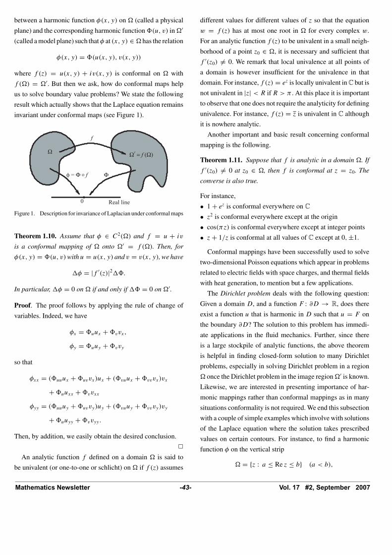
invariant under conformal maps (see Figure 1).

Figure 1. Description for invariance of Laplacian under conformal maps

Theorem 1.10. Assume that φ ∈ C2(�) and f = u + iv

is a conformal mapping of � onto �′ = f (�). Then, for

φ(x, y) = (u, v) with u = u(x, y) and v = v(x, y), we have

�φ = |f ′(z)|2�.

In particular, �φ = 0 on � if and only if � = 0 on �′.

Proof. The proof follows by applying the rule of change of

variables. Indeed, we have

φx = uux + vvx,

φy = uuy + vvy

so that

φxx = (uuux + uvvx)ux + (vuux + vvvx)vx

+ uuxx + vvxx

φyy = (uuuy + uvvy)uy + (vuuy + vvvy)vy

+ uuyy + vvyy.

Then, by addition, we easily obtain the desired conclusion.

�

An analytic function f defined on a domain � is said to

be univalent (or one-to-one or schlicht) on � if f (z) assumes

different values for different values of z so that the equation

w = f (z) has at most one root in � for every complex w.

For an analytic function f (z) to be univalent in a small neigh-

borhood of a point z0 ∈ �, it is necessary and sufficient that

f ′(z0) �= 0. We remark that local univalence at all points of

a domain is however insufficient for the univalence in that

domain. For instance, f (z) = ez is locally univalent in C but is

not univalent in |z| < R if R > π . At this place it is important

to observe that one does not require the analyticity for defining

univalence. For instance, f (z) = z is univalent in C although

it is nowhere analytic.

Another important and basic result concerning conformal

mapping is the following.

Theorem 1.11. Suppose that f is analytic in a domain �. If

f ′(z0) �= 0 at z0 ∈ �, then f is conformal at z = z0. The

converse is also true.

For instance,

• 1 + ez is conformal everywhere on C

• z2 is conformal everywhere except at the origin

• cos(πz) is conformal everywhere except at integer points

• z + 1/z is conformal at all values of C except at 0, ±1.

Conformal mappings have been successfully used to solve

two-dimensional Poisson equations which appear in problems

related to electric fields with space charges, and thermal fields

with heat generation, to mention but a few applications.

The Dirichlet problem deals with the following question:

Given a domain D, and a function F : ∂D → R, does there

exist a function u that is harmonic in D such that u = F on

the boundary ∂D? The solution to this problem has immedi-

ate applications in the fluid mechanics. Further, since there

is a large stockpile of analytic functions, the above theorem

is helpful in finding closed-form solution to many Dirichlet

problems, especially in solving Dirichlet problem in a region

� once the Dirichlet problem in the image region �′ is known.

Likewise, we are interested in presenting importance of har-

monic mappings rather than conformal mappings as in many

situations conformality is not required. We end this subsection

with a couple of simple examples which involve with solutions

of the Laplace equation where the solution takes prescribed

values on certain contours. For instance, to find a harmonic

function φ on the vertical strip

� = {z : a ≤ Re z ≤ b} (a < b),


with φ(a, y) = A and φ(b, y) = B, a natural choice is to set

u(x, y) = ax + b.

It is easy to see that the required solution is given by

φ(x, y) = A + A − B

a − b(x − a).

Here is another problem which follows from the derivation of

the equation governing the steady-state temperature distribu-

tion φ(x, y).

Example 1.12. Suppose that we wish to determine electro-

static potential φ on the domain � between the circles |z| = 1

and |z − 1/2| = 1/2 such that (see Figure 2)

φ(x, y) = −10 on |z| = 1 and

φ(x, y) = 20 on |z − 1/2| = 1/2.

Clearly, our aim is to find a harmonic function φ on � satisfy-

ing the given boundary conditions. In applying Theorem 1.10

to find such a φ, one must know a conformal map which trans-

forms � onto the image the domain �′ for which many explicit

solutions to a Dirichlet problem are known. For instance, in

our problem we may transform � into a horizontal infinite

strip by choosing i �→ 0, −1 �→ 1, 1 �→ ∞. This can be done

by a Mobius transformation. Indeed, the well-known invari-

ance property of the cross ratio immediately yields that (see

for example [18, 19])

f (z) = (1 − i)z − i

z − 1.

Note that 1 is common to the both the circles so that f (∂D) =R ∪ {∞} and f (∂D(1/2, 1/2)) is the extended line with ∞,

namely, the line v = 1 with the point at ∞. The boundary

conditions are transformed to

(u, v) = −10 on v = 0, and (u, v) = 20 on v = 1.

Figure 2. A conformal mapping between a domain and a strip

Now, we introduce (u, v) = a + bv. Using the transformed

new boundary conditions, we compute a and b and obtain

(u, v) = 30v − 10 = 30 Im (f (z)) − 10.

This gives

φ(x, y) = 30

(1 − (x2 + y2)

(1 − x)2 + y2

)− 10

which is a desired solution to our problem. •

When log z is suitably restricted, it becomes analytic and

hence, we have a pair of two harmonic functions (real and

imaginary parts), i.e. log z = ln |z| + i arg z. We observe that

ln |z| is constant on circles centered at the origin. In view of

this observation and the idea of the above example, it is easy to

find a steady state temperature distribution φ in � consisting

of points outside of the two circles |z−5/2| = 1/2 and |z| = 1

such that φ equals 30 on the unit circle |z| = 1 and φ vanishes

on the circle |z − 5/2| = 1/2. We leave this problem as a

simple exercise.

1.13. Canonical Representation

Recall from (1.3) that the Cauchy–Riemann equations in carte-

sian form can be equivalently written in a single concise equa-

tion: fz = 0. Often this is referred to as the complex form of

Cauchy–Riemann equations. Moreover, it is a simple exercise

to see that the Laplacian of f becomes

�f = 4∂

∂z

(∂f

∂z

)= 0, � = 4

∂2

∂z∂z,

which is referred to as the complex form of Laplace equation.

Thus, we have equivalent formulation of Definition 1.1.

Definition 1.14. We say that a complex valued function f is

harmonic if and only if f ∈ C2(�) with �f = 4fzz = 0.

There is a close interrelation between analytic functions and

harmonic functions. For example, if we use the formula �f =4fzz, then we conclude the following:

Proposition 1.15. f is necessarily independent of z for ana-

lytic functions f whereas fz is independent of z for planar

harmonic functions f .

From this proposition, we observe that the function f with

continuous partial derivatives is harmonic in a planar domain


� if and only if fz is analytic in �. Also, if f is analytic in �

then fz(z) = f ′(z) in �. We now present our first basic result

for harmonic functions.

Lemma 1.16 (Canonical Representation). Let � be a sim-

ply connected domain in C. Then f : � → C is a (planar)

harmonic function if and only if the function f has the repre-

sentation f = h + g, where h and g are analytic in �. The

representation is unique up to an additive constant. We call

the functions h and g the analytic and the co-analytic parts of

f , respectively.

Proof. Set f = u + iv, where u and v both are harmonic in

a simply connected plane domain �. Then there exist analytic

functions F and G on � such that

u = Re F = F + F

2and v = Im G = G − G

2i.

This observation gives the representation

f = F + F

2+ G − G

2=(

F + G

2

)+(

F − G

2

):= h + g,

where both h and g are clearly analytic in �, and g denotes

the function z �→ g(z).

Alternately, suppose that f is harmonic. Then, fz is analytic

in the simply connected domain �, and so we may define h

by h′ = fz, where h is analytic in � and h is determined up to

an additive constant. To obtain the desired representation for

known f and h, we define g by

g = f − h = f − h

so that f = h + g. It suffices to show that g is analytic in �,

i.e. gz = 0. Now

gz = ∂

∂z(f − h) = fz − hz = fz − h′ = 0 in �,

and thus, g is analytic in �. The converse part is obvious.

The uniqueness follows from the fact that a function which

is both analytic and anti-analytic1 is constant. �

Remark 1.17. If the function f in Lemma 1.16 is real-valued,

then f may be expressed as f = h + h = 2Re h so that 2h

represents the analytic completion of f and is unique up to an

additive imaginary constant. •1Conjugate of an analytic function is called an anti-analytic

function.

1.18. Composition Rule for Harmonic Functions

In the linear space H(�) of analytic functions in �, analytic

functions are preserved under product and composition rules,

but harmonic functions are not. For example, the functions x

and x2 show that the product of two harmonic functions is not

necessarily harmonic.

Proposition 1.19.

(1) If f : � → C, g : f (�) → C are harmonic functions,

g ◦ f is not necessarily harmonic.

(2) If f : � → C is analytic and g : f (�) → C is harmonic,

then g ◦ f is harmonic.

(3) If f : � → C is harmonic and g : f (�) → C is analytic,

then g ◦ f is not necessarily harmonic.

Proof. We leave the proof as an exercise to the reader. �

At this place, it is important to emphasize that the class of

harmonic functions is not conformally invariant. In particular,

inverse or square of a harmonic function need not be harmonic.

2. Harmonic Mappings

A complex-valued harmonic function f : � → C is said to be

a harmonic mapping if it is univalent (one-to-one) in �, i.e.

f (z1) �= f (z2) for all z1, z2 ∈ � with z1 �= z2.

Thus, (planar) harmonic mappings are univalent complex-

valued functions whose real and imaginary parts are not nec-

essarily conjugate, i.e. do not need to satisfy the Cauchy–

Riemann equations. Thus, every conformal or anti-conformal

mapping f on a domain � is a harmonic mapping. In particu-

lar, the class of (planar) harmonic mappings on the unit disk D

includes the subclass of univalent functions that are also ana-

lytic in D, a popular topic in geometric function theory (see

[7, 9, 17]).

Example 2.1. Consider f : C → C by f (z) = 4x + i4xy.

Then, f is a harmonic function. Also, we easily have the

decomposition

f = h + g, h(z) = 2z + z2, g(z) = 2z − z2.

Is this a harmonic mapping? If not, how about the same func-

tion when it is restricted to the right half-plane � = {z :

Re z > 0}? Does the inverse exist on �? Must the inverse be

a harmonic mapping on �?


2.2. Jacobian and Local Univalence

The Jacobian of a function f = u + iv at a point z is defined

to be

Jf (z) =∣∣∣∣∣ux vx

uy vy

∣∣∣∣∣ = uxvy − uyvx,

which may be expressed equivalently in terms of z- and z-

derivatives

Jf (z) = |fz|2 − |fz|2.

Iff is analytic on�, thenfz(z) = 0 on� and sofz(z) = f ′(z).Thus, the Jacobian takes the form

Jf (z) = (ux)2 + (vx)

2 = |f ′(z)|2.

Let f be an univalent function defined on a domain � and

belong to C1(�) such that Jf (z) �= 0 in �. Then f is said to be

a diffeomorphism or more accurately, a C1-diffeomorphism of

� onto its range. We remark that, if f : � → C is a diffeomor-

phism, then either Jf (z) > 0 everywhere in � or Jf (z) < 0

throughout the domain �. This follows from the fact that �

is connected and Jf : � → R is a continuous and zero-free

function, i.e. the set {Jf (z) : z ∈ �} is a connected set of

real numbers that does not contain zero and hence, Jf (�) is

either a subset of (−∞, 0) or a subset of (0, ∞). When Jf is

positive in �, then the diffeomorphism f is called orientation-

preserving mapping or sense-preserving mapping. A diffeo-

morphism with a negative Jacobian is said to be orientation-

reversing mapping or sense-reversing mapping. We see that

the conjugate f of a diffeomorphism f : � → C is also a dif-

feomorphism, i.e. the one for which

Jf (z) = −Jf (z).

Therefore, f is orientation-reversing when f is orientation-

preserving, and vice versa. For example, in the unit disk D,

(1) f (z) = z is sense-preserving, as Jf (z) = 1 in D.

(2) f (z) = (1 + z)2 is sense-preserving, as Jf (z) = |2(1 +z)|2 > 0 in D.

(3) f (z) = z is sense-reversing, as Jz(z) = −1 < 0 in D.

A well-known classical result for analytic functions states

that an analytic function f is locally univalent at z0 if and

only if Jf (z0) �= 0 (see for example, [19, Theorems 11.2 and

11.3]). In 1936, Hans Lewy [16] showed that this remains true

for harmonic functions.

Theorem 2.3 (Lewy’s Theorem). A harmonic function f is

locally univalent in a neighborhood of z0 if and only if

Jf (z0) �= 0. That is, f is locally univalent in a domain � if

and only if Jf (z) �= 0 throughout �.

An immediate consequence of Lemma 1.16 and Theo-

rem 2.3 is the following.

Corollary 2.4. Let f be a complex-valued harmonic function

on a simply connected domain � with the decomposition f =h + g. Then f is locally univalent and sense-preserving in �

if and only if |h′(z)| > |g′(z)| in �. Equivalently, f is a sense-

preserving local homeomorphism if and only if Jf (z) > 0.

The set of all critical points of a C1-function consists of

those points where the Jacobian vanishes. Thus, for a harmonic

function f , the set of critical points consists of those points

for which f is not locally univalent.

Remark 2.5. Lewy’s theorem does not hold for harmonic

mappings in higher dimensions (n ≥ 3). The following exam-

ple is due to Wood [23]. Consider f : R3 → R3 by

f (x, y, z) = (x3 − 3xz2 + yz, y − 3xz, z).

The three coordinate functions u = x3 − 3xz2 + yz, v =y−3xz, w = z are harmonic as they satisfy the 3-dimensional

Laplace equation: �u = 0 = �v = �w, where

� = ∂2

∂x2+ ∂2

∂y2+ ∂2

∂z2.

Thus, the function f is harmonic in R3. The Jacobian of the

given function is

Jf (x, y, z) =

∣∣∣∣∣∣∣∣

3x2 − 3z2 −3z 0

z 1 0

−6xz + y −3x 1

∣∣∣∣∣∣∣∣= 3x2.

To find the inverse function, we need to solve x and y in terms

of u, v, w. Substituting z = w, the expression for u and v

becomes

u = x3 + w(y − 3xw) and v = y − 3xw.

Using the second equation, the first one may be rewritten as

u = x3 + vw or x = 3√

u − vw

and so v = y − 3xw gives

y = v + 3w3√

u − vw.


Thus, the inverse function f −1 : R3 → R3 is given by

f −1(u, v, w) = (3√

u − vw, v + 3w3√

u − vw, w).

Thus, the given function is a homeomorphism of R3 but the

Jacobian vanishes on the plane x = 0. �

2.6. Harmonic Mappings on the Plane C

For entire functions (analytic in C), it is well-known that the

only univalent analytic self mappings of C are the linear map-

pings of the form f (z) = a0 + a1z, where a0, a1 are constants

with a1 �= 0 (see for example [18] and [19]). It is natural to

ask the harmonic analog of this result.

Theorem 2.7. [6] The only harmonic mappings of C onto C

are the affine mappings f (z) = αz + γ + βz, where α, β and

γ are complex constants and |α| �= |β|.

Proof. Let f map C harmonically onto C. Then f has the

form

f = h + g,

where h and g are entire functions, and we may assume without

loss of generality that f is sense-preserving. As f is sense-

preserving, we have |g′(z)| < |h′(z)| in C and so g′/h′, being

a bounded entire function, reduces to a constant (by Liouville’s

theorem). Consequently, g′(z) ≡ bh′(z) so that integration

gives

g(z) = bh(z) + c

for some complex constants b and c with |b| < 1. Thus, f

reduces to the form

f (z) = h(z) + b h(z) + c.

Setting w = h(z), we may write

f (z) = F(h(z)) = (F ◦ h)(z) with F(w) = w + bw + c.

Note that F is an (invertible) affine mapping. It follows that

h = F−1 ◦ f is analytic and maps C univalently onto C, and

so h(z) = a0 + a1z, where a0, a1 are complex constants with

a1 �= 0. This shows that f has the form

f (z) = a0 + a1z + b(a0 + a1z) + c,

which is the affine mapping in the desired form. �

Theorem 2.7, in particular, shows that there exists no har-

monic mapping of C onto a proper sub domain � of C. Also,

we remark that the simplest example of sense-preserving har-

monic mapping on the plane that is not necessarily conformal

is an affine mapping

f (z) = αz + βz, |α| > |β| > 0.

Example 2.8. For n ≥ 1, consider (compare with

Lemma 1.16)

fn(z) = z + n

n + 1z.

Then, each fn is a harmonic mapping in C (and in particular, in

the unit disk D). Note that {fn} converges uniformly to f (z) =z + z which is clearly not a harmonic mapping, see Figure 3.

What does this mean? •

Figure 3. Image of unit disk under fn(z) = z + (n/(n + 1))z forn = 1, 2, 3, 4

Example 2.9. Consider

f (z) = z − 1

z+ 2 ln |z|.

Then it is easy to see that f is a harmonic mapping on the

exterior � = C \ D of the unit disk D onto the punctured

complex plane C \ {0}. Note that f (∂D) is simply the origin.

We write

f = h + g, h(z) = z + log z and g(z) = −1

z+ log z

and note that h and g are not (globally) analytic on

C \ D which is not simply connected in C. So, we

require an analog of Lemma 1.16 for multiply connected

domains. �


2.10. Connections to Quasiconformal Mappings

Let f : � → f (�) be a sense-preserving C1-diffeomorphism,

z0 ∈ �, and w = f (z) = u(z)+iv(z). By using the properties

of the differential operators from advanced calculus, we obtain

du = uxdx + uydy, dv = vxdx + vydy,

which may be written in the form

dw = df = fzdz + fz dz.

Since f is a diffeomorphism, it is locally linear (in this case at

z0). Indeed, the affine map L defined by

L(z) := fz(z0)dz + fz(z0)dz

sends a circle with center 0 in the dz-plane onto an ellipse in

the dw-plane, with major axis of length L = |fz(z0)|+|fz(z0)|and minor axis of length l = |fz(z0)| − |fz(z0)|. It follows

that

(|fz| − |fz|)|dz| ≤ |dw| ≤ (|fz| + |fz|)|dz|

where both the limits are attained. The differential dw maps

the circle |dz| = r onto the ellipse, see Figure 4. The ratio

Df (z) between the major and the minor axes is

Df := |fz| + |fz||fz| − |fz| ≥ 1.

This quantity Df (z) is called dilatation of f at the point z ∈ �.

Figure 4. Image of the circle |dz| = r under the differential map dw.

Definition 2.11. A sense-preserving diffeomorphism f is said

to be K-quasiconformal, if Df (z) ≤ K throughout the given

region �, where K ∈ [1, ∞) is a constant.

We define the quantity df (z) as follows:

df := |fz||fz| < 1,

because, for sense-preserving maps, |fz| > |fz|. Thus, we

have

Df (z) = 1 + df (z)

1 − df (z)and df (z) = Df (z) − 1

Df (z) + 1. (2.12)

We may use Df as a measure of the local distortion of the

mapping f at z. Now we define complex dilatation µf by

µf = fz

fz

with |µf | = df . (2.13)

Thus, by (2.12) and (2.13), the two dilatations µf and Df are

related by

|µf (z)| = Df (z) − 1

Df (z) + 1.

If ∂αf (z) denotes the directional derivative of a C1-mapping

f in a direction making an angle α with the positive x-

direction, then

∂αf (z) = limr→0

f (z + reiα) − f (z)

reiα

= e−iα limr→0

{u(x+r cos α, y+r sin α) − u(x, y)

r

+iv(x + r cos α, y + r sin α) − v(x, y)

r

}.

Adding and subtracting terms u(x, y + r sin α) and v(x, y +r sin α) in the numerators of the first and the second terms on

the right, respectively, we obtain

∂αf (z) = e−iα[(ux cos α + uy sin α)

+i(vx cos α + vy sin α)]

= e−iα[fx cos α + fy sin α]

= e−iα[(fz + fz) cos α + i(fz − fz) sin α]

= e−iα[fzeiα + fze

−iα]

= fz + fze−2iα

= fz

[1 + fz

fz

e−2iα

]for fz �= 0.

Hence, for a sense-preserving C1-map f between planar

domains, we have

�f (z) := maxα

|∂αf (z)| = |fz(z)| + |fz(z)| and

λf (z) := minα

|∂αf (z)| = |fz(z)| − |fz(z)|.


It is an easy exercise to see that if z1 �= 0, then

|z1 + z2| = |z1| + |z2| ⇐⇒ arg(z2/z1) = 0

and similarly,

|z1 + z2| = |z1| − |z2| ⇐⇒ arg(z2/z1) = ±π.

Therefore the maximum is attained provided that

arg

(fz

fz

e−2iα

)= 0, i.e. α = 1

2arg

(fz

fz

).

Thus, the maximum corresponds to the direction

arg dz = α = 1

2arg µf

and the minimum in the orthogonal direction

arg dz = β = α ± π

2.

We define the quantity ω := νf of f by

ω(z) := νf (z) = fz(z)

fz(z).

The function νf (z) is called the second complex dilatation

which turns out to be more natural than the first complex dilata-

tion µf . Because |νf | = |µf |, f is quasiconformal if and only

if |νf (z)| ≤ k < 1. Finally, we remark that

Df ≤ K ⇔ df ≤ k := K − 1

K + 1.

The mapping f is conformal if and only if µf (z) = 0 on �,

i.e. fz vanishes identically on �. From our notation, ∂αf (z) is

then independent of α so that

∂αf (z) = fz(z) = f ′(z).

This is equivalent to the dilatation quotient being identically

equal to 1. Thus, f is conformal if and only if Df = 1 and

µf = 0. If K is defined by

K = supz∈�

Df = supz∈�

1 + |µf (z)|1 − |µf (z)|

is bounded, then we call f a K-quasiconformal mapping of

� to f (�). We call K the maximal dilatation of f and it is a

finite number ≥ 1. Sometimes, f is called a K-quasiconformal

mapping with the Beltrami coefficient µf .

The simplest example of quasiconformal mapping is given

by the affine mapping

f (z) = az + bz (a, b ∈ C, |b| < |a|);

for fz = a, fz = b, |µf | = |b|/|a| and f maps the unit circle

to an ellipse, and the ratio of the major and minor axes of this

ellipse is

K = |a| + |b||a| − |b| = 1 + |µf |

1 − |µf |As another example, we consider

f (z) ={

z if z ∈ U = {w : Re (w) > 0},x + iky if z ∈ C \ U, k > 1.

Then fz = 1 and fz = 0 if z ∈ U. If z ∈ C \ U, then we may

rewrite f as

f (z) = z + z

2+ ik

(z − z

2i

)

so that

fz = 1 + k

2and fz = 1 − k

2.

Thus,

Df = (1 + k)/2 + (k − 1)/2

(1 + k)/2 − (k − 1)/2= k

and hence, f is a K-quasiconformal mapping of C with K = k.

What is important about quasiconformal mappings? We first

recall the following facts:

(1) Quasiconformal maps are considered to be a natural gen-

eralization of conformal maps.

(2) In many of the results on conformal mappings, one

requires just the quasi-conformality and hence, it is of

interest to know when conformality is necessary and when

it is not.

(3) Quasiconformal maps behave less rigidly than conformal

maps and thus can be used as a tool in complex analysis.

(4) Later development shows that the class of quasiconformal

mappings play an important role in the study of elliptic

partial differential equations.

(5) Extremal problems in quasiconformal mappings lead to

analytic functions connected with regions or Riemann sur-

faces.

(6) The family of conformal mappings degenerates to Mobius

transformations when generalized to several variables, but

the family of quasiconformal mappings is interesting in

the higher dimensions also (see [21])

There are many areas in which quasiconformal mappings are

used. As a general reference to the theory of quasiconformal


mappings in plane, we refer to [2, 14, 15] and we would con-

sider the topic at a later stage. For the higher dimensional the-

ory, we refer to the books of Vaisala [21] and Vuorinen [22]

although at this stage it is too early for us to discuss higher

dimensional results. However, it might be useful to recall the

problem of Grotzsch with two simple examples of quasicon-

formal mappings in the plane.

Problem 2.14. Let Q be a square and R be a rectangle not

a square. In 1928, H. Grotzsch, posed the following problem:

Does there exist a conformal mapping of Q onto R which maps

vertices onto vertices?

Because of the extra condition that the vertices mapping

onto vertices, the Riemann mapping theorem does not guar-

antee existence of such a mapping and so the problem of

Grotzsch is interesting in itself. It is this extra condition

that led us to the development of the theory of quasicon-

formal mappings. Actually, there does not exist a confor-

mal mapping of Q onto R taking vertices onto vertices and

hence, the question is to find most nearly conformal map-

ping of this kind, and this needs a measure of approximate

conformality.

2.15. Solutions of Elliptic PartialDifferential Equation

Suppose that f is a harmonic mapping defined on a simply

connected domain �. Then, because f has the form f = h+g

and f is univalent in �, we have

Jf = |fz|2 − |fz|2 = |h′|2 − |g′|2 �= 0.

Thus, f is either sense-preserving or sense-reversing. In the

first case, Jf (z) > 0, i.e. |h′(z)| > |g′(z)| throughout �.

Note that in the second case, f is sense-preserving. In the

case of sense-preserving harmonic mappings, we have the

following

Theorem 2.16. Let f ∈ C2(�) with Jf (z) > 0 on �. Then

the function f is harmonic on � if and only if f is the solution

of the elliptic partial differential equation

fz(z) = ω(z)fz(z), z ∈ �, (2.17)

for some analytic function ω on � with |ω(z)| < 1 on �.

Proof. ⇒: Suppose that f (= h+g) is a harmonic function

with Jf (z) > 0 on �. Then, as fz(z) = h′(z) �≡ 0 and fz(z) =g′(z), we can define a function ω(z) by

ω(z) := νf (z) = g′(z)h′(z)

= fz(z)

fz(z)

which is analytic on � and |ω(z)| < 1 on �, because Jf =|h′|2 −|g′|2 > 0. The desired form (2.17) follows from the last

relation.

⇐: Conversely, suppose that f is a C2-solution of (2.17)

with Jf (z) > 0 on �. Differentiating the equation (2.17) with

respect to z, one finds

fzz(z) = ω(z)fzz(z) + ωz(z)fz(z)

so that fzz = ωfzz as ωz = 0. Further, as |ω(z)| < 1, we have

fzz(z) = 0 and therefore, f is harmonic on �. �

Note that if the second complex dilatation ω of a har-

monic mapping f on the domain � satisfies |ω(z)| ≤k < 1 in �, then f is a quasiconformal with the max-

imum dilatation K = (1 + k)/(1 − k); i.e. f is a K-

quasiconformal.

Corollary 2.18. Sense-preserving harmonic mappings are

locally quasiconformal.

Example 2.19. For n ≥ 2, consider the function

f (z) = z − 1

nzn.

For each n ≥ 2, the function f is harmonic and has the

second complex dilatation ω(z) = −zn−1 (apply for exam-

ple, Theorem 2.16). To verify its univalence in D, suppose

f (z1) = f (z2) for z1, z2 ∈ D. Then, we have

n(z1 − z2) = z1n − z2

n = (z1 − z2)

× (z1n−1 + z1

n−2z2 + · · · + z2n−1).

By taking absolute values on both sides, we see that this

is impossible unless z1 = z2 because |z1n−1 + z1

n−2z2 +· · · + z2

n−1| < n. Thus, f is a harmonic mapping of the

open unit disk D onto the domain bounded by a hypocycloid

of n + 1 cusps, inscribed in the circle |w| = (n + 1)/n.

Note also that F(z) = z + 1nzn is analytic and univalent in

D because |F ′(z) − 1| < 1 in for all z ∈ D. Thus, F is

a normalized univalent function in D. The images of f and

F for n = 2 are illustrated in Figures 5 and 6 whereas the

images of f and F for n = 4 are illustrated in Figures 7

and 8. �


Figure 5. Image of D under f (z) = z − 12 z2

Figure 6. Image of D under F(z) = z + 12 z2

Figure 7. Image of D under f (z) = z − 14 z4

2.20. Normalizations

Suppose that f is a harmonic mapping of a proper simply

connected domain � of C. By the Riemann mapping theorem

Figure 8. Image of D under F(z) = z + 14 z4

there is a conformal mapping ϕ of D onto �. It follows that

the composition f ◦ ϕ maps D harmonically onto �. As a

consequence of this observation, we may assume that � is the

unit disk and that f is sense-preserving in D. We next observe

that, because Jf = |h′|2 − |g′|2 > 0 for the sense-preserving

harmonic mapping f = h + g, fz(0) = h′(0) �= 0, and so we

arrive at the normalized form of f :

f (z) − f (0)

fz(0).

Thus, the analytic and co-analytic parts of the harmonic map-

ping f = h + g in D may be written, respectively,

h(z) = z +∞∑

n=2

anzn and g(z) =

∞∑n=1

bnzn.

Definition 2.21. Let SH denote the class of all complex-

valued (sense-preserving) harmonic mappings that are nor-

malized on the unit disk D. That is,

SH = {f : D → C : f is harmonic and univalent with

f (0) = 0 = fz(0) − 1}.

We note that SH reduces to S, the class of normalized univa-

lent analytic functions in D whenever the co-analytic part of f

is zero, i.e. g(z) ≡ 0 in D. Furthermore, for f = h + g ∈ SH ,

|b1| < 1 (because Jf (0) = 1 − |g′(0)|2 = 1 − |b1|2 > 0) and

therefore, the function

F = f − b1f

1 − |b1|2 (2.22)

is also in SH . Note that this function is obtained by apply-

ing an affine mapping to f . Thus, we may sometimes restrict


our attention to the subclass of functions f in SH for which

b1 = fz(0) = 0. We define

S0H = {f ∈ SH : fz(0) = 0}.

Note that the condition fz(0) = 0 is equivalent to ω(0) = 0 or

g(z) = O(z2) for z near the origin, where ω(z) is the second

complex dilatation of f . Clearly,

S � S0H � SH .

Although both SH and S0H are known to be normal families

[i.e. every sequence of functions in SH (resp. S0H ) has a sub-

sequence that converges locally uniformly in D] only S0H is

compact with respect to the topology of locally uniform con-

vergence (see [6]). Indeed, SH is not a compact family because

it is not preserved under passage to locally uniform limits. The

limit function is necessarily harmonic in D, but it need not be

univalent. For example, the sequence of affine mappings fn

defined in Example 2.8 demonstrates that SH is not a compact

family.

Identifying z = x + iy ∈ C with (x, y) ∈ R2 and points in

R2 as 2×1 column matrix, we may rewrite the equation (2.22)

in matrix form as

(1 − |b1|2)(

Re F

Im F

)=(

1 − b1 0

0 1 + b1

)(Re f

Im f

)

and so, pre-multiplying by the inverse of the 2×2 matrix gives

(Re f

Im f

)=(

1 + b1 0

0 1 − b1

)(Re F

Im F

).

Simplifying the last relation reveals that the transformation

(2.22) is one-to-one and its inverse is given by

f = F + b1F .

This observation enables us to derive a number of properties

about SH and S0H , [6].

2.23. Method of shearing

One of the forms of constructing harmonic mappings, intro-

duced by Clunie and Sheil-Small [6], is known as “shear

construction.” This method produces certain planar harmonic

mappings by adjoining functions in S with co-analytic parts

that are related to or derived from analytic parts. Moreover,

in this method one produces a harmonic mapping of D with a

specified dilatation onto a domain in one direction by “shear-

ing” a conformal mapping along parallel lines.

Definition 2.24. A domain � is convex in the direction eiα , if

for every fixed complex number a, the set �∩{a+teiα : t ∈ R}is either connected or empty; i.e. every line parallel to the line

through 0 and eiα has a connected intersection with �.

In particular, it is convenient to consider domains convex

in the direction of the real axis (denoted by CHD). Thus, a

domain � is a CHD if every line parallel to the real axis has

a connected intersection with �. Clearly, a domain � in C is

convex if and only if it is convex in every direction.

Definition 2.25. A function f defined in D is said to be CHD

if its range is CHD; i.e. if the intersection of f (D) with each

horizontal line is connected.

For example, the Koebe function k(z) = z/(1 − z)2, and

the convex function c(z) = z/(1 − z) are univalent in D and

CHD. The following lemma due to Clunie and Sheil-Small [6]

is a basis for the construction of harmonic mappings that are

convex in the direction of the real axis, in particular.

Lemma 2.26. For analytic functions h and g, assume that

f = h + g is harmonic and locally univalent in the unit disk

D. Then f is a univalent mapping of D onto a CHD domain

if and only if h − g is a conformal mapping of D onto a CHD

domain.

Remark 2.27.

(1) From Lemma 2.26, we note that the imaginary part of

the analytic function h − g equals the imaginary part of

the harmonic function f = h + g so that the domain

is changed or cut or stretched in the real direction.

In view of this observation, the method is known as

“shearing”.

(2) Lemma 2.26 indeed holds for simply connected domains

rather than for functions defined on the unit disk D.

(3) From the definition, it is clear that the harmonic mapping

f = h + g has a convex range if and only if the range

is convex in every direction. That is equivalent to saying

that the range of every rotation eiαf (z) (= eiαh+e−iαg)

is CHD, for 0 ≤ α < 2π . •


One can use the technique of shear construction for con-

structing interesting examples of harmonic mappings by shear-

ing conformal mappings with a prescribed dilatation ω(z). As a

simple demonstration, let φ be a conformal mapping of the unit

disk D onto a CHD domain with φ(0) = 0, and let f = h + g

be a sense-preserving harmonic function, where h and g are

analytic in D. Then the dilatation ω = g′/h′ is analytic with

|ω(z)| < 1 in D. According to the shear technique, the con-

struction of harmonic mappings proceeds by letting h−g = φ.

This gives the pair of linear differential equations

h′(z) − g′(z) = φ′(z) and ω(z)h′(z) − g′(z) = 0.

Solving for h′(z) and g′(z), and then integrating with the nor-

malization g(0) = h(0) = 0, we arrive at the formulas for h

and g explicitly:

h(z) =∫ z

0

φ′(t)1 − ω(t)

dt and

g(z) =∫ z

0

ω(t)φ′(t)1 − ω(t)

dt = h(z) − φ(z).

So, the shear construction produces the harmonic mapping f

defined by

f (z) = h(z) + g(z) = 2Re h(z) − φ(z)

and f maps D onto a CHD domain. Various choices of the

dilatation ω(z) and the conformal mapping φ(z) produce a

number of harmonic mappings, as demonstrated by a number

of examples below (see the paper by Greiner [10] for many

more examples).

Example 2.28. Note that z − z3/3 maps D onto a domain

which is convex in the direction of the real axis and so is the

harmonic function f = h + g, where

h − g = z − 1

3z3 and

g′(z)h′(z)

= z2 (= ω(z)).

As h′(z) − g′(z) = 1 − z2 and g′(z) = z2h′(z), solving these

two equations yields that

h′(z) = 1 and g′(z) = z2.

As h(0) − g(0) = 0, i.e. g(0) = h(0), it follows that

h(z) = z and g(z) = 1

3z3

which gives

f (z) = h(z) + g(z) = z + 1

3z3.

The harmonic mappingf maps D onto the interior of the region

bounded by the hypocycloid with 4 cusps. Also, we note that

h(z)−g(z) is a conformal mapping of D onto the interior of an

epicycloid with 2 cusps. The geometric behaviors of f (z) =z + 1

3z3 and F(z) = z − 13z3 are illustrated in Figures 9 and

10. •

Figure 9. Image of D under f (z) = z + 13 z3

Figure 10. Image of D under F(z) = z − 13 z3

Example 2.29. Let h − g = k with the dilatation ω(z) = z,

where k(z) = z/(1 − z)2 is the Koebe function. This gives the

pair of differential equations

h′(z) − g′(z) = 1 + z

(1 − z)3and g′(z) = zh′(z).


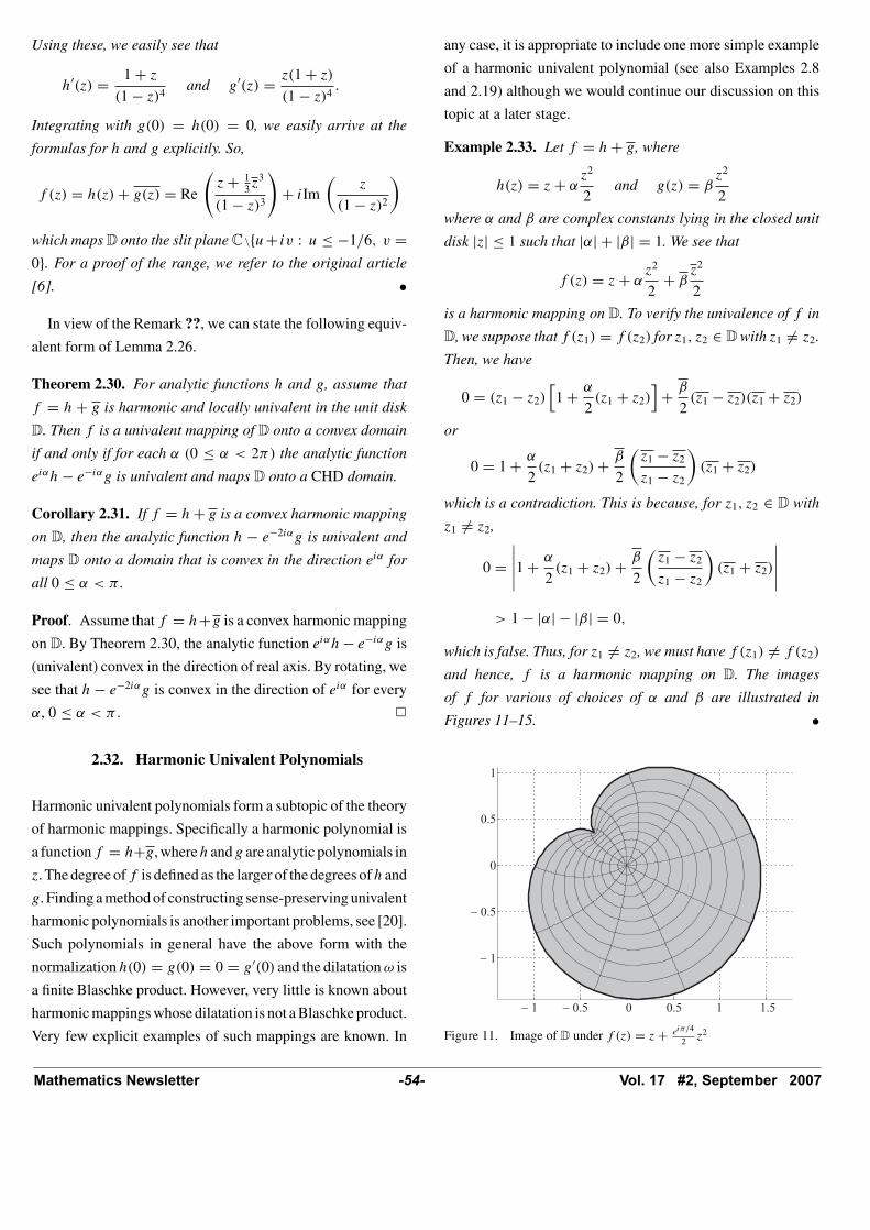
Using these, we easily see that

h′(z) = 1 + z

(1 − z)4and g′(z) = z(1 + z)

(1 − z)4.

Integrating with g(0) = h(0) = 0, we easily arrive at the

formulas for h and g explicitly. So,

f (z) = h(z) + g(z) = Re

(z + 1

3z3

(1 − z)3

)+ iIm

(z

(1 − z)2

)

which maps D onto the slit plane C \{u+ iv : u ≤ −1/6, v =0}. For a proof of the range, we refer to the original article

[6]. •

In view of the Remark ??, we can state the following equiv-

alent form of Lemma 2.26.

Theorem 2.30. For analytic functions h and g, assume that

f = h + g is harmonic and locally univalent in the unit disk

D. Then f is a univalent mapping of D onto a convex domain

if and only if for each α (0 ≤ α < 2π) the analytic function

eiαh − e−iαg is univalent and maps D onto a CHD domain.

Corollary 2.31. If f = h + g is a convex harmonic mapping

on D, then the analytic function h − e−2iαg is univalent and

maps D onto a domain that is convex in the direction eiα for

all 0 ≤ α < π .

Proof. Assume that f = h+g is a convex harmonic mapping

on D. By Theorem 2.30, the analytic function eiαh − e−iαg is

(univalent) convex in the direction of real axis. By rotating, we

see that h − e−2iαg is convex in the direction of eiα for every

α, 0 ≤ α < π . �

2.32. Harmonic Univalent Polynomials

Harmonic univalent polynomials form a subtopic of the theory

of harmonic mappings. Specifically a harmonic polynomial is

a functionf = h+g, whereh andg are analytic polynomials in

z. The degree off is defined as the larger of the degrees ofh and

g. Finding a method of constructing sense-preserving univalent

harmonic polynomials is another important problems, see [20].

Such polynomials in general have the above form with the

normalization h(0) = g(0) = 0 = g′(0) and the dilatation ω is

a finite Blaschke product. However, very little is known about

harmonic mappings whose dilatation is not a Blaschke product.

Very few explicit examples of such mappings are known. In

any case, it is appropriate to include one more simple example

of a harmonic univalent polynomial (see also Examples 2.8

and 2.19) although we would continue our discussion on this

topic at a later stage.

Example 2.33. Let f = h + g, where

h(z) = z + αz2

2and g(z) = β

z2

2

where α and β are complex constants lying in the closed unit

disk |z| ≤ 1 such that |α| + |β| = 1. We see that

f (z) = z + αz2

2+ β

z2

2

is a harmonic mapping on D. To verify the univalence of f in

D, we suppose that f (z1) = f (z2) for z1, z2 ∈ D with z1 �= z2.

Then, we have

0 = (z1 − z2)[1 + α

2(z1 + z2)

]+ β

2(z1 − z2)(z1 + z2)

or

0 = 1 + α

2(z1 + z2) + β

2

(z1 − z2

z1 − z2

)(z1 + z2)

which is a contradiction. This is because, for z1, z2 ∈ D with

z1 �= z2,

0 =∣∣∣∣∣1 + α

2(z1 + z2) + β

2

(z1 − z2

z1 − z2

)(z1 + z2)

∣∣∣∣∣> 1 − |α| − |β| = 0,

which is false. Thus, for z1 �= z2, we must have f (z1) �= f (z2)

and hence, f is a harmonic mapping on D. The images

of f for various of choices of α and β are illustrated in

Figures 11–15. •

Figure 11. Image of D under f (z) = z + eiπ/4

2 z2


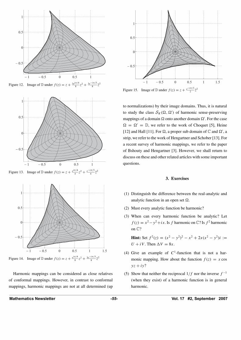
Figure 12. Image of D under f (z) = z + 3eiπ/4

8 z2 + 3e−iπ/3

8 z2


4 z2 + e−iπ/3

4 z2


8 z2 + 3e−iπ/3

8 z2

Harmonic mappings can be considered as close relatives

of conformal mappings. However, in contrast to conformal

mappings, harmonic mappings are not at all determined (up

Figure 15. Image of D under f (z) = z + e−iπ/3

2 z2

to normalizations) by their image domains. Thus, it is natural

to study the class SK(�, �′) of harmonic sense-preserving

mappings of a domain � onto another domain �′. For the case

� = �′ = D, we refer to the work of Choquet [5], Heine

[12] and Hall [11]. For �, a proper sub domain of C and �′, a

strip, we refer to the work of Hengartner and Schober [13]. For

a recent survey of harmonic mappings, we refer to the paper

of Bshouty and Hengartner [3]. However, we shall return to

discuss on these and other related articles with some important

questions.

3. Exercises

(1) Distinguish the difference between the real-analytic and

analytic function in an open set �.

(2) Must every analytic function be harmonic?

(3) When can every harmonic function be analytic? Let

f (z) = x2 −y2 +ix. Is f harmonic on C? Is f 2 harmonic

on C?

Hint: Set f 2(z) = (x2 − y2)2 − x2 + 2x(x2 − y2)i :=U + iV . Then �V = 8x.

(4) Give an example of C1-function that is not a har-

monic mapping. How about the function f (z) = x cos

yz + iy?

(5) Show that neither the reciprocal 1/f nor the inverse f −1

(when they exist) of a harmonic function is in general

harmonic.


(6) Consider the automorphism of the unit disk: φa(z) =eiθ (z − a)/(1 − az) (|a| < 1). If f : D → D

is a harmonic function, must φa ◦ f be harmonic in

D?

(7) Show that the composition of a harmonic mapping with

an affine mapping is harmonic, i.e. if f is harmonic, then

so is αf + βf + γ , |α| �= |β|.(8) Verify whether the composition of a harmonic function

with a conformal premapping is a harmonic function.

(9) Suppose that f (z) = ln |z| + iy. Determine �, analytic

functions h and g so that the decomposition f (z) =h(z) + g(z) Is possible. Also determine the correspond-

ing second complex dilatation ω(z) which is analytic in

� with |ω(z)| < 1 for z ∈ �.

(10) For |α| ≤ 2, let fα(z) = z − 1z+ α ln |z|. Show that each

fα is sense-preserving harmonic mapping of the exterior

of the unit disk onto the punctured plane.

Hint: See [13].

(11) State and prove the composition rule for (f ◦ g)z and

(f ◦ g)z.

(12) Suppose that f is a harmonic function in an open set

� ⊆ C such that Jf (z0) �= 0 at some point z0 ∈ �.

Show that f is either sense-preserving or sense-reversing

in some neighbourhood of z0.

(13) Suppose that f is a sense-preserving harmonic mapping

of a domain �. Must |fz| > 0 on �? Must the second

complex dilatation ω(z) be an analytic mapping of � into

the unit disk D?

(14) Suppose that f is an sense-preserving (reversing) har-

monic diffeomorphism and g is analytic (anti-analytic).

Verify whether the Jacobian of f ◦g does not change sign,

i.e. Jf ◦g > 0 (< 0).

(15) Modify Remark 2.5 to obtain a harmonic homeomor-

phism of Rn with Jacobian vanishing on a hyper-

plane. Conclude that Lewy’s theorem is false for all

n ≥ 3.

(16) If f (z) = z + z2 − z, determine the critical points of f

in C.

(17) Verify whether the following functions are harmonic in

the upper half-plane � = {z = x + iy : y > 0}:

(a) f (z) = arg z + iy

(b) f (z) = xy + iy.

Are these mappings take � onto �. If not find f (�).

(18) Must f (z) = z + Re (ez) be a harmonic mapping in

C?

(19) Let f = h + g with h + g = z/(1 − z) and with the

dilatation ω(z) = −z (Note that z/(1 − z) is convex

in every direction). Compute the formulas for h and g

explicitly and determine f (D).

(20) Does Example 2.9 follow from Lemma 1.16 or Corollary

2.4? If yes, explain. If not, could you find an analog of

Corollary 2.4 applicable to Example 2.9?

(21) Define f (z) = z|z| 1k−1 for k ≥ 1. Is f a quasiconformal

mapping of C with K = k?

(22) Let f = h + g with h − g = z. Assume first the

dilatation ω(z) = z and then ω(z) = z2. Using the

shear construction, determine f in each case. Find also

f (D).

(23) Let f = h + g be a CHD domain. Must fα defined by

fα = h + eiαg convex in the direction eiα?

References

[1] L. V. Ahlfors, Complex Analysis, 2nd ed., McGraw-

Hill, New York, 1966.

[2] L. V. Ahlfors, Lectures on Quasiconformal Map-

pings, Second edition. With supplemental chapters by

C. J. Earle, I. Kra, M. Shishikura and J. H. Hubbard.

University Lecture Series, 38. American Mathematical

Society, Providence, RI, 2006. viii+162 pp.

[3] D. Bshouty and W. Hengartner, Univalent har-

monic mappings in the plane, In: Handbook of Complex

Analysis: Geometric Function Theory, Vol. 2 (2005),

479–506, Edited by R. Kuhnau (ISBN: 0-444-51547-

X), Elsevier.

[4] R. B. Burckel, An introduction to Classical Complex

Analysis, Vol. I, Academic Press, 1979.

[5] G. Choquet, Sur un type de transformation analytique

generalisant la representation conforme et definie au

moyen de fonctions harmoniques, Bull. Sci. Math. 69

(1945), 156–165.


[6] J. G. Clunie and T. Sheil-Small, Harmonic univa-

lent functions, Ann. Acad. Sci. Fenn. Ser. A.I. 9 (1984),

3–25.

[7] P. L. Duren, Univalent Functions (Grundlehren der

mathematischen Wissenschaften 259, New York,

Berlin, Heidelberg, Tokyo), Springer-Verlag,

1983.

[8] P. Duren, Harmonic Mappings in the Plane, Cambridge

University Press, 2004.

[9] A. W. Goodman, Univalent Functions, Vols. I and II.

Mariner Publishing Co. Tampa, Florida, 1983.

[10] P. Greiner, Geometric properties of harmonic shears,

Comput. Methods Funct. Theory 4 (2004), no. 1, 77–96.

[11] R. R. Hall, On an inequality of E. Heinz, J. Analyse

Math. 42 (1983), 185–198.

[12] E. Heinz, Uber die Losungen der Mini-

malflachengleichung, Nachr. Akad. Wiss. Gottingen,

Math.-Phys. K1. (1952), 51–56.

[13] W. Hengartner, and G. Schober, Univalent har-

monic mappings, Trans. Amer. Math. Soc. 299 (1987),

1–31.

[14] O. Lehto, Univalent functions and Teichmuller spaces,

Graduate Texts in Mathematics, 109. Springer-Verlag,

New York, 1987.

[15] O. Lehto and K. I. Virtanen, Quasiconformal map-

pings in the plane, Second edition. Translated from the

German by K. W. Lucas. Die Grundlehren der mathe-

matischen Wissenschaften, Band 126. Springer-Verlag,

New York-Heidelberg, 1973.

[16] H. Lewy, On the nonvanishing of the Jacobian in cer-

tain one-to-one mapppings, Bull. Amer. Math. Soc. 42

(1936), 689–692.

[17] Ch. Pommerenke, Univalent Functions, Gottingen:

Vandenhoeck & Ruprecht, 1975.

[18] S. Ponnusamy, Foundations of Complex Analysis,

Alpha Science International Publishers, UK, 2005.

[19] S. Ponnusamy and H. Silverman, Complex Variables

with Applications, Birkhauser, Boston, 2006.

[20] T. J. Suffridge, Harmonic univalent polynomials,

Complex Variables Theory Appl. (2)35 (1998), 93–107.

[21] J. Vaisala, Lectures on n-dimensional quasiconformal

mappings, Lecture Notes in Math. Vol. 229, Springer-

Verlag, 1971.

[22] M. Vuorinen, Conformal geometry and quasiregular

mappings. (Monograph, 208 pp.). Lecture Notes in

Math. Vol. 1319, Springer-Verlag, 1988.

[23] J. C. Wood, Lewy’s theorem fails in higher dimensions,

Math. Scand. 69 (1991), 166.


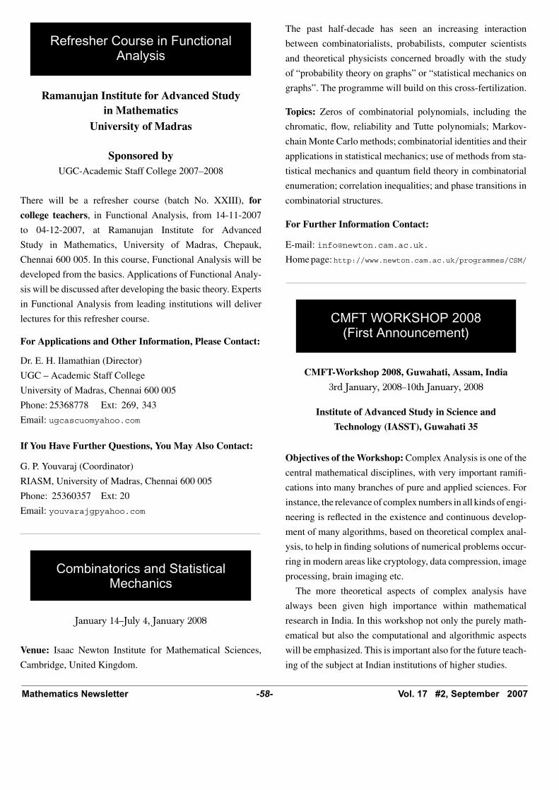
Refresher Course in FunctionalAnalysis

Ramanujan Institute for Advanced Studyin Mathematics

University of Madras

Sponsored byUGC-Academic Staff College 2007–2008

There will be a refresher course (batch No. XXIII), for

college teachers, in Functional Analysis, from 14-11-2007

to 04-12-2007, at Ramanujan Institute for Advanced

Study in Mathematics, University of Madras, Chepauk,

Chennai 600 005. In this course, Functional Analysis will be

developed from the basics. Applications of Functional Analy-

sis will be discussed after developing the basic theory. Experts

in Functional Analysis from leading institutions will deliver

lectures for this refresher course.

For Applications and Other Information, Please Contact:

Dr. E. H. Ilamathian (Director)

UGC – Academic Staff College

University of Madras, Chennai 600 005

Phone: 25368778 Ext: 269, 343

Email: ugcascuomyahoo.com

If You Have Further Questions, You May Also Contact:

G. P. Youvaraj (Coordinator)

RIASM, University of Madras, Chennai 600 005

Phone: 25360357 Ext: 20

Email: youvarajgpyahoo.com

Combinatorics and StatisticalMechanics

January 14–July 4, January 2008

Venue: Isaac Newton Institute for Mathematical Sciences,

Cambridge, United Kingdom.

The past half-decade has seen an increasing interaction

between combinatorialists, probabilists, computer scientists

and theoretical physicists concerned broadly with the study

of “probability theory on graphs” or “statistical mechanics on

graphs”. The programme will build on this cross-fertilization.

Topics: Zeros of combinatorial polynomials, including the

chromatic, flow, reliability and Tutte polynomials; Markov-

chain Monte Carlo methods; combinatorial identities and their

applications in statistical mechanics; use of methods from sta-

tistical mechanics and quantum field theory in combinatorial

enumeration; correlation inequalities; and phase transitions in

combinatorial structures.

For Further Information Contact:

E-mail: [email protected].

Home page: http://www.newton.cam.ac.uk/programmes/CSM/

CMFT WORKSHOP 2008(First Announcement)

CMFT-Workshop 2008, Guwahati, Assam, India

3rd January, 2008–10th January, 2008

Institute of Advanced Study in Science and

Technology (IASST), Guwahati 35

Objectives of the Workshop: Complex Analysis is one of the

central mathematical disciplines, with very important ramifi-

cations into many branches of pure and applied sciences. For

instance, the relevance of complex numbers in all kinds of engi-

neering is reflected in the existence and continuous develop-

ment of many algorithms, based on theoretical complex anal-

ysis, to help in finding solutions of numerical problems occur-

ring in modern areas like cryptology, data compression, image

processing, brain imaging etc.

The more theoretical aspects of complex analysis have

always been given high importance within mathematical

research in India. In this workshop not only the purely math-

ematical but also the computational and algorithmic aspects

will be emphasized. This is important also for the future teach-

ing of the subject at Indian institutions of higher studies.


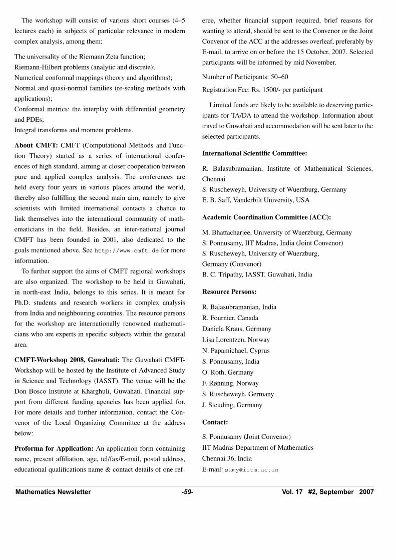
The workshop will consist of various short courses (4–5

lectures each) in subjects of particular relevance in modern

complex analysis, among them:

The universality of the Riemann Zeta function;

Riemann-Hilbert problems (analytic and discrete);

Numerical conformal mappings (theory and algorithms);

Normal and quasi-normal families (re-scaling methods with

applications);

Conformal metrics: the interplay with differential geometry

and PDEs;

Integral transforms and moment problems.

About CMFT: CMFT (Computational Methods and Func-

tion Theory) started as a series of international confer-

ences of high standard, aiming at closer cooperation between

pure and applied complex analysis. The conferences are

held every four years in various places around the world,

thereby also fulfilling the second main aim, namely to give

scientists with limited international contacts a chance to

link themselves into the international community of math-

ematicians in the field. Besides, an inter-national journal

CMFT has been founded in 2001, also dedicated to the

goals mentioned above. See http://www.cmft.de for more

information.

To further support the aims of CMFT regional workshops

are also organized. The workshop to be held in Guwahati,

in north-east India, belongs to this series. It is meant for

Ph.D. students and research workers in complex analysis

from India and neighbouring countries. The resource persons

for the workshop are internationally renowned mathemati-

cians who are experts in specific subjects within the general

area.

CMFT-Workshop 2008, Guwahati: The Guwahati CMFT-

Workshop will be hosted by the Institute of Advanced Study

in Science and Technology (IASST). The venue will be the

Don Bosco Institute at Kharghuli, Guwahati. Financial sup-

port from different funding agencies has been applied for.

For more details and further information, contact the Con-

venor of the Local Organizing Committee at the address

below:

Proforma for Application: An application form containing

name, present affiliation, age, tel/fax/E-mail, postal address,

educational qualifications name & contact details of one ref-

eree, whether financial support required, brief reasons for

wanting to attend, should be sent to the Convenor or the Joint

Convenor of the ACC at the addresses overleaf, preferably by

E-mail, to arrive on or before the 15 October, 2007. Selected

participants will be informed by mid November.

Number of Participants: 50–60

Registration Fee: Rs. 1500/- per participant

Limited funds are likely to be available to deserving partic-

ipants for TA/DA to attend the workshop. Information about

travel to Guwahati and accommodation will be sent later to the

selected participants.

International Scientific Committee:

R. Balasubramanian, Institute of Mathematical Sciences,

Chennai

S. Ruscheweyh, University of Wuerzburg, Germany

E. B. Saff, Vanderbilt University, USA

Academic Coordination Committee (ACC):

M. Bhattacharjee, University of Wuerzburg, Germany

S. Ponnusamy, IIT Madras, India (Joint Convenor)

S. Ruscheweyh, University of Wuerzburg,

Germany (Convenor)

B. C. Tripathy, IASST, Guwahati, India

Resource Persons:

R. Balasubramanian, India

R. Fournier, Canada

Daniela Kraus, Germany

Lisa Lorentzen, Norway

N. Papamichael, Cyprus

S. Ponnusamy, India

O. Roth, Germany

F. Rønning, Norway

S. Ruscheweyh, Germany

J. Steuding, Germany

Contact:

S. Ponnusamy (Joint Convenor)

IIT Madras Department of Mathematics

Chennai 36, India



Stephan Ruscheweyh (Convenor)

University of Wuerzberg

Institute of Mathematics 97074

Wuerzburg, Germany

E-Mail: [email protected]

B. C. Tripathy (Convenor, Local)

Institute of Advanced Study in Science & Technology,

Paschim Boragaon

Mathematical Sciences Division

Guwahati 781 035,

Assam, India

E-Mail: [email protected]

Phone: 9864087231

Ramanujan Mathematical Society

“RMS Lecture Notes Series in Mathematics”

Field Office:- 8/1,13th Cross, Adipampa Road

V. V. Mohalla, Mysore 570 002

India

Sponsored by

The Department of Science and Technology

Government of India, New Delhi

RMS LECTURE NOTES SERIES provides an outlet for pub-

lication of a vast amount of recent and relevant materials gen-

erated through important developments taking place in Math-

ematics, Mathematical Sciences (Pure Mathematics, Opera-

tions Research, Statistics & Theoretical Computer Science)

and allied areas anywhere in the world, especially

• Proceedings of conferences and instructional workshops

which focus on a topic of current research and

• Monographs which consist of notes from seminars, lecture

series, tutorials, courses and exposition of important topics

by eminent scholars for which there are no readily available

textbooks.

The manuscripts submitted for possible publication in this

series will undergo a screening process as the emphasis of

the series rests on standards and high quality of mathematical

content. Though it is not mandatory, it is expected that the

proposal will meet a part of the cost of printing. This will

facilitate to give around 40 copies of the proceedings to the

editor(s) free of cost.

Individual Coordinators/institutions where events such as

those mentioned above have taken place, or are about to take

place in the near future, are encouraged to submit two hard

copies of the manuscripts in LATEX pdf formats along with a

Compact Disc (CD) copy at the address cited above.

Distribution and/or marketing rights for the volumes under

the series would be exclusively with the Ramanujan Mathe-

matical Society (RMS).

National Conference on AppliedMathematics (NCOAM 2008)

3–4 January, 2008

Organizer:

Department of Mathematics

B. S. Abdur Rahman Crescent Engineering College

Vandalur, Chennai 600 048

Important Dates:

Submission of Full paper : 30/09/2007

Confirmation of selection : 15/10/2007

Camera Ready paper and

Conference registration : 31/10/2007

Address for Correspondence:

The Co-ordinator

NCOAM 2008


B. S. Abdur Rahman Crescent Engineering College

Vandalur, Chennai 600 048

Phone No: 22751347/48/75 Extn. 393

E-mail: ncoam [email protected]

Web site: www.crescentcollege.org


International Conference onFunctional Analysis And its

Applications (FAA 2007)

November 28–December 1, 2007

Call for Papers: Researchers/Teachers who wish to present

papers in the conference are encouraged to send their

abstract in any area of Functional Analysis (a few are listed

below) preferably in Tex or MS word pdf file by E-mail to

[email protected] latest by October 25, 2007.

Abstracts sent by post will also be accepted.

Important Dates:

Abstract submission : October 25, 2007

Registration : October 31, 2007

Submission of the full tex

of the paper in Tex format : December 31, 2007

For More Details Contact:

J. R. V. Edward

Organizing Secretary, FAA 2007


Scott Christian College (Autonomous)

Nagercoil 629 003, Tamil Nadu, India.

E-mail Id: [email protected]

[email protected]

Cell no: (0)9443605698

Home page:

http://www.scottchristian.org/faa2007/home.asp


Irreducibility of Polynomials Whose Coefﬁcients are Integersthanga/papers/mnl.pdf ·...

Documents

Transcript of Irreducibility of Polynomials Whose Coefﬁcients are Integersthanga/papers/mnl.pdf ·...