Irene Torres Espallardo - Instituto de Física...
186
Consejo Superior de Investigaciones Científicas Universitat de València IFIC - INSTITUTO DE FISICA CORPUSCULAR IMAGE RECONSTRUCTION AND CORRECTION METHODS FOR MADPET-II BASED ON MONTE CARLO TECHNIQUES Irene Torres Espallardo Departament de F´ ısica At`omica, Molecular y Nuclear, IFIC Universitat de Val` encia - CSIC
Transcript of Irene Torres Espallardo - Instituto de Física...

Consejo Superior de Investigaciones CientíficasUniversitat de València
IFIC - INSTITUTO DE FISICA CORPUSCULAR
IMAGE RECONSTRUCTION AND
CORRECTION METHODS
FOR MADPET-II BASED ON
MONTE CARLO TECHNIQUES
Irene Torres Espallardo
Departament de Fısica Atomica, Molecular y Nuclear, IFIC
Universitat de Valencia - CSIC


Magdalena Rafecas Lopez, Investigadora Ramon y Cajal del Departamentode Fısica Atomica, Molecular y Nuclear de la Universitat de Valencia, y
Sibylle I. Ziegler, Investigadora jefe del grupo de Instrumentacion de laNuklearmedizinische Klinik und Poliklinik, Klinikum rechts der Isar der Technis-che Universitat Munchen en Munich (Alemania)
Certifican:
Que la presente memoria, IMAGE RECONSTRUCTION AND CORRECTION METHODS
FOR MADPET-II BASED ON MONTE CARLO TECHNIQUES, ha sido realizada bajo su di-reccion en la Nuklearmedizinische Klinik und Poliklinik, Klinikum rechts der Isarder Technischen Universitat Munchen y el Instituto de Fısica Corpuscular deValencia por Irene Torres Espallardo, y constituye su Tesis para optar al gradode Doctora en Ciencias Fısicas.
Y para que ası conste, en cumplimiento de la legislacion vigente, presentanen la Universitat de Valencia la referida Tesis Doctoral, y firman el presentecertificado, en
Burjassot, 1 de Diciembre de 2009
Magdalena Rafecas Lopez Sibylle I. Ziegler

Contents
Prologo 9
Introduccion sobre PET dedicados a animales pequenos 13
1 Small Animal PET scanners 231.1 Basics of PET . . . . . . . . . . . . . . . . . . . . . . . . . . . . . 23
1.1.1 Instrumentation . . . . . . . . . . . . . . . . . . . . . . . . 231.1.2 Image Reconstruction . . . . . . . . . . . . . . . . . . . . . 291.1.3 Image Degradation and Compensation . . . . . . . . . . . 491.1.4 Image Quality . . . . . . . . . . . . . . . . . . . . . . . . . 571.1.5 Monte Carlo Simulations . . . . . . . . . . . . . . . . . . . 58
1.2 Why small animal PET scanners? . . . . . . . . . . . . . . . . . . 631.3 Challenges of small animal PET . . . . . . . . . . . . . . . . . . . 631.4 Overview of this work . . . . . . . . . . . . . . . . . . . . . . . . 65
2 MADPET-II 672.1 Objectives of the system . . . . . . . . . . . . . . . . . . . . . . . 672.2 System Description . . . . . . . . . . . . . . . . . . . . . . . . . . 682.3 Image Reconstruction . . . . . . . . . . . . . . . . . . . . . . . . . 72
2.3.1 Simulations with GATE . . . . . . . . . . . . . . . . . . . 73
3 System Matrix for MADPET-II 753.1 Monte Carlo System Matrix . . . . . . . . . . . . . . . . . . . . . 753.2 Generation of the System Matrices . . . . . . . . . . . . . . . . . 76
3.2.1 Matrix Symmetries . . . . . . . . . . . . . . . . . . . . . . 783.2.2 Use of Grid . . . . . . . . . . . . . . . . . . . . . . . . . . 783.2.3 Storage of the System Matrix . . . . . . . . . . . . . . . . 79
3.3 Characterization of the System Matrices . . . . . . . . . . . . . . 803.4 Effect of the Low Energy Threshold on Image Reconstruction . . 81
3.4.1 Simulated Sources . . . . . . . . . . . . . . . . . . . . . . . 813.4.2 Image reconstruction . . . . . . . . . . . . . . . . . . . . . 833.4.3 Figures-of-Merit . . . . . . . . . . . . . . . . . . . . . . . . 83
3.5 Results: Comparison of the System Matrices . . . . . . . . . . . . 833.5.1 Characteristics of the System Matrices . . . . . . . . . . . 833.5.2 Sensitivity Matrix . . . . . . . . . . . . . . . . . . . . . . . 85
5

3.5.3 Spatial Resolution . . . . . . . . . . . . . . . . . . . . . . 863.5.4 Quantification . . . . . . . . . . . . . . . . . . . . . . . . . 90
3.6 Conclusions . . . . . . . . . . . . . . . . . . . . . . . . . . . . . . 94
4 Random Coincidences Correction 974.1 Randoms Estimation Methods for MADPET-II . . . . . . . . . . 97
4.1.1 Approaches to the Delayed Window method . . . . . . . . 984.1.2 Simulations to study the performance . . . . . . . . . . . . 984.1.3 Figures-of-Merit . . . . . . . . . . . . . . . . . . . . . . . . 100
4.2 Results . . . . . . . . . . . . . . . . . . . . . . . . . . . . . . . . . 1014.2.1 Overestimation of the Random Coincidences . . . . . . . . 1014.2.2 Effect of the Inter-Crystal Scatter . . . . . . . . . . . . . . 1044.2.3 Including triple random coincidences . . . . . . . . . . . . 1054.2.4 Quantification of the reconstructed activities . . . . . . . . 1074.2.5 Effect of the activity . . . . . . . . . . . . . . . . . . . . . 112
4.3 Conclusions . . . . . . . . . . . . . . . . . . . . . . . . . . . . . . 118
5 Triple Coincidences 1215.1 Triple Coincidences in MADPET-II . . . . . . . . . . . . . . . . . 1225.2 System Matrix for the triple coincidences . . . . . . . . . . . . . . 1225.3 Random estimation method . . . . . . . . . . . . . . . . . . . . . 124
5.3.1 Delayed Window method . . . . . . . . . . . . . . . . . . . 1245.3.2 Singles Rate method . . . . . . . . . . . . . . . . . . . . . 125
5.4 Simulated sources . . . . . . . . . . . . . . . . . . . . . . . . . . . 1265.5 Figures of merit . . . . . . . . . . . . . . . . . . . . . . . . . . . . 1275.6 Results and Discussion . . . . . . . . . . . . . . . . . . . . . . . . 127
5.6.1 Characterization of System Matrices . . . . . . . . . . . . 1275.6.2 Effect on spatial resolution . . . . . . . . . . . . . . . . . . 1295.6.3 Random coincidences correction . . . . . . . . . . . . . . . 131
5.7 Conclusions . . . . . . . . . . . . . . . . . . . . . . . . . . . . . . 133
6 Normalization Correction 1376.1 Normalization for to MADPET-II . . . . . . . . . . . . . . . . . . 138
6.1.1 Calculation of the normalization factors . . . . . . . . . . 1386.1.2 How to apply the normalization . . . . . . . . . . . . . . . 1406.1.3 Normalization source . . . . . . . . . . . . . . . . . . . . . 141
6.2 Effect on Image Reconstruction . . . . . . . . . . . . . . . . . . . 1436.2.1 Measured Phantoms . . . . . . . . . . . . . . . . . . . . . 1436.2.2 Figure-of-Merit: Relative Error . . . . . . . . . . . . . . . 143
6.3 Results . . . . . . . . . . . . . . . . . . . . . . . . . . . . . . . . . 1446.3.1 Efficiency Coefficients . . . . . . . . . . . . . . . . . . . . . 1446.3.2 Validity of the proposed methods . . . . . . . . . . . . . . 146
6.4 Conclusions . . . . . . . . . . . . . . . . . . . . . . . . . . . . . . 147
Conclusiones 159
6

List of Abbreviations 165
Bibliography 169
7


Prologo
La memoria que se presenta a continuacion recoge el trabajo de investigacionllevado a cabo entre el Klinikum rechts der Isar y el Instituto de Fısica Corpus-cular de Valencia para optar al grado de doctora en Ciencias Fısicas. El trabajose enmarca dentro del campo de Imagen Medica y mas concretamente en el detomografos PET dedicados a animales pequenos.
Bajo el tıtulo Reconstruccion de la Imagen y Correcciones para MADPET-IIusando Tecnicas de Montecarlo hemos englobado diversos temas relacionados conla obtencion de imagenes y correcciones necesarias para obtener informacion cuan-titativa del escaner MADPET-II. En particular se han investigado las correccionesde coincidencias accidentales y la normalizacion para dicho sistema. MADPET-II, que viene de Munich Avalanche photoDiode PET, es un escaner para el estu-dio de animales pequenos desarrollado en el departamento de Medicina Nucleardel Klinikum rechts der Isar en Munich. Sus rasgos mas caracterısticos son ladistribucion de los cristales centelleadores en dos capas radiales y la lectura indi-vidual de cada uno de sus cristales por un fotodiodo de avalancha (APD). En elcapıtulo 2 se discute con mas detalle y profundidad el diseno y las caracterısticasde este escaner. MADPET-II permite obtener una alta sensibilidad, manteniendouna alta resolucion espacial. La alta sensibilidad se consigue usando un campode vision (FOV) tan grande como el diametro interno del escaner, reduciendo elumbral energetico e introduciendo sucesos triples1, producidos cuando uno de losfotones ha depositado su energıa en mas de un cristal. Al mismo tiempo, se lograuna alta resolucion espacial porque se proporciona informacion de la profundi-dad de interaccion del foton en el cristal (DOI) y las imagenes son reconstruıdasusando algoritmos iterativos tridimensionales basados en histogramas de lıneasde respuesta, junto con una matriz del sistema generada a traves de tecnicasMontecarlo. Dos capıtulos de esta tesis se han reservado al estudio de dos de loselementos mencionados previamente, la creacion de una matriz del sistema basadaen Montecarlo (capıtulo 3) y la introduccion de los sucesos triples (capıtulo 5).
En general, los escaneres PET para animales pequenos se dedican a estudiosradiofarmaceuticos. En este tipo de estudios es muy importante que las imagenes
1Un foton de 511 keV puede depositar toda su energıa en un cristal o a traves de sucesivasinteracciones Compton ir dejando la energıa en diferentes cristales. Gracias a la lectura indi-vidual de los cristales de MADPET-II y cuando la energıa depositada en los distintos cristalescae dentro de la ventana energetica, es posible detectar mas de un suceso asociado con un solofoton. Por tanto, se puede producir y detectar un suceso triple proveniente de los dos fotonesde la aniquilacion.
9

10
reconstruıdas proporcionen informacion cuantitativa sobre la actividad emitidapor el sujeto en estudio. Varias correcciones se deben de aplicar para obtenerestimaciones realistas de la distribucion de actividad. Entre estas correcciones,esta tesis se ha centrado en la correccion debida a las coincidencias aleatorias(capıtulo 4) y la normalizacion (capıtulo 6).
Todos los capıtulos de esta tesis tienen un denominador comun que es el usode simulaciones basadas en tecnicas Montecarlo. Nos hemos beneficiado de lasventajas que ofrecen las tecnicas de Montecarlo, pero tambien hemos sufrido suslimitaciones. Empezando con las ventajas, hemos podido simular un escanercuya geometrıa es bastante compleja debido a su configuracion en doble capa.Otra ventaja de las tecnicas de Montecarlo es que permite estudiar efectos deparametros que no pueden ser medidos en la practica. Particularizando paranuestro caso, gracias a esta capacidad pudimos validar los metodos para la es-timacion de las coincidencias aleatorias usando la informacion relacionada conla aniquilacion que proporciona el programa de simulacion. Ademas, como esun modelo computacional, es posible activar o desactivar ciertos efectos segunnuestros intereses. Por ejemplo, en las simulaciones para el estudio de las coin-cidencias aleatorias no fueron incluidas la dispersion y la atenuacion debidas alobjeto, para podernos centrar en los efectos debidos al sistema y a los detectores.En cambio, para el estudio de normalizacion, necesitamos una simulacion lo mascercana posible a la medida de normalizacion, por tanto, simulamos la fuentedentro de el continente de plastico, incluyendo la atenuacion y la dispersion delobjeto, junto con la atenuacion de la actividad con el tiempo. Una limitacionimportante de las tecnicas Montecarlo es el tiempo de computacion necesariopara hacer una simulacion. Para resolver este problema hemos recurrido a lassimetrıas del escaner y a la granja de ordenadores que hay en la instalacion deGrid en el IFIC.
Despues de los capıtulos de introduccion y de la descripcion del escanerMADPET-II, el esquema de este trabajo se presenta a continuacion:
• Capıtulo 3 presenta la generacion de la matriz del sistema basada en lastecnicas de Monte Carlo.
• Capıtulo 4 investiga la estimacion y correccion de coincidencias aleatorias.
• Capıtulo 5 incluye los sucesos triples para obtener imagenes.
• Capıtulo 6 estudia diferentes propuestas para la normalizacion.
Al final de cada capıtulo se encuentran las correspondientes conclusiones.Estas se encuentran resumidas en el ultimo capıtulo en castellano. Por tanto,salvo la introduccion a PET dedicados a animales pequenos que viene a contin-uacion y las conclusiones finales, el resto de la tesis esta escrita en ingles. De estaforma se cumplen los requisitos exigidos por la normativa del Doctorado Europeo.

A mis queridos padres,Pepe y Virtudes,por sus continuos animos.


Breve Introduccion sobre
tomografos PET dedicados a
animales pequenos
La tomografıa por emision de positrones, Positron Emission Tomography (PET),es una tecnica de diagnostico por imagen que usa sustancias radiactivas paraobtener imagenes fisiologicas del cuerpo. Entre otros, las imagenes de PETpueden visualizar el metabolismo de la glucosa, el flujo sanguıneo o concentra-ciones de receptores. Con estas imagenes se puede detectar tumores, localizarareas del corazon afectadas por enfermedad coronaria o identificar zonas del cere-bro afectadas por drogas. Por esta razon, las imagenes que se obtienen a travesde la PET se llaman funcionales, a diferencia de otras, como la tomografıa com-puterizada, que produce imagenes anatomicas.
El primer paso en un estudio de PET es la produccion del radiofarmaco apropi-ado para visualizar la enfermedad en cuestion. El radiofarmaco es una sustanciaformada por radionuclidos emisores de positrones (los mas usados son 15O, 13N,11C y 18F) incorporados a moleculas biologicamente interesantes para el estudioa realizar. Posteriormente, el radiofarmaco se introduce en el cuerpo, bien porinyeccion o inhalacion. La calidad de las imagenes mejora con la cantidad de ra-diofarmaco administrado, pero la radiacion que reciben los organos internos delpaciente pone un lımite a la dosis administrada. El radioisotopo con el que se hamarcado el radiofarmaco emite positrones y estos se aniquilan emitiendo dos fo-tones de 511 keV en la misma direccion y sentidos opuestos. Estas emisiones salendel cuerpo del paciente en todas las direcciones a una tasa proporcional a la con-centracion local de radioarmaco, y son detectados por el sistema PET, que rodeaal paciente. El sistema de adquisicion guarda la informacion sobre la posicion ydireccion del par de fotones que se ha detectado. Estos datos se organizan en his-togramas, donde cada bin corresponde a una pareja de detectores. El histogramaresultante contiene medidas de las proyecciones. Las imagenes tomograficas no sepueden ver directamente, sino que se calculan a partir de las proyecciones en unproceso llamado reconstruccion de la imagen. El metodo convencional de recon-struccion de la imagen es una tecnica llamada retroproyeccion filtrada de Fourier,Fourier filtered backprojection (FBP). La FBP es una tecnica de reconstruccionanalıtica, es decir, la solucion a la reconstruccion se puede escribir explıcitamente.Esto es posible gracias a que estos metodos no consideran el ruido estadıstico, ni
13

14
otros factores fısicos que complican la descripcion del proceso de imagen. Frente alas tenicas analıticas, en los ultimos anos, han emergido las denominadas tecnicasiterativas, como los algoritmos Maximum-Likelihood Expectation-Maximization(MLEM) y Ordered-Subsets Expectation-Maximization (OS-EM). Los metodositerativos, que se usan para implementar estimaciones estadısticas, permiten in-cluir en el proceso de reconstruccion factores que describen la emision y detecciondel par de fotones, produciendo imgenes de PET de mayor calidad.
La PET, como otras tecnicas de diagnostico a traves de la imagen, se estausando en laboratorios con animales pequenos. Una de las ventajas que ofrece laPET es que permite utilizar el mismo animal varias veces, pues no es necesariosacrificar el animal, como por ejemplo en la autorradiografıa. Esta ventaja esimportante ya que se evitan variaciones debidas a diferencias entre distintos an-imales de la misma especie, tambien permite el seguimiento de una terapia y elestudio de la evolucion de una enfermedad. El resultado final es que se reduce elnumero de animales usados en el laboratorio, se acelera la obtencion de resultadosy se mejora la calidad de los resultados.
Un gran numero de compuestos marcados con emisores de positrones se hansintetizado [8] abriendo la posibilidad a que se puedan medir cuantitativamente unamplio rango de procesos biologicos no invasıvamente y repetidamente con PET.Combinado junto con la alta especificidad de los radiotrazadores, permite poderestudiar encimas especıficos, proteınas, receptores y genes, haciendo la tecnicaPET tremendamente atractiva para estudios en laboratorios con animales. Porultimo, otra gran ventaja de usar la PET con animales pequenos (para hacermodelos de enfermedades) es que las imagenes producidas proporcionan un puenteentre el modelo del animal y estudios con humanos. El raton se ha convertido enel animal elegido para crear modelos de enfermedades humanas y para intentarentender la biologıa de los mamıferos. Esto se debe, fundamentalmente, a quelos ratones tienen una alta tasa de reproduccion y que genetica y fisiologicamenteson similares a los humanos. Para estudios cerebrales, tradicionalmente se hautilizado la rata por el tamano de su cerebro (3.3 g el de la rata y 0.45 g el delraton).
Hay un gran numero de cuestiones que se deben de considerar cuidadosa-mente en el caso de los estudios PET con animales pequenos. Algunas de ellasson comunes al diseno y optimizacion de escaneres PET para humanos; otras,son especıficas de este tipo de escaneres. El objetivo fundamental es obtenerel mayor numero de cuentas posible y localizarlas con tanta precision como seaposible. El determinar con exactitud la posicion donde se ha generado el parde fotones depende, fundamentalmente, de la resolucion espacial de los detec-tores y de la habilidad para quitar o corregir sucesos dispersados, coincidenciasaleatorias y otros fenomenos fısicos de degradacion de la imagen. Aumentar elnumero de cuentas detectadas requiere aumentar la dosis suministrada, hasta lle-gar a un maximo que vendra determinado por la masa del animal y la actividadespecıfica del radiofarmaco. Tambien se pueden aumentar los sucesos detectadosaumentando la eficiencia de los detectores y cubriendo el maximo angulo solido.
En cuanto a la resolucion espacial, la diferencia fundamental entre un escaner

15
PET para humanos y uno dedicado a animales pequenos viene de los diferentestamanos fısicos entre humanos (70 kg) y ratas o ratones (30-300 g). Por tanto,para alcanzar la misma calidad de imagen, la resolucion espacial se ha de mejo-rar en comparacion con la que tiene un escaner PET de humanos. Si se tieneuna resolucion espacial de 10 mm en estudios de cuerpo entero con escaneresclınicos, se ha de obtener una resolucion en la imagen menor de 1 mm en todaslas direcciones para los estudios con animales.
La sensibilidad absoluta de deteccion del sistema de imagen, es decir, lafraccion de desintegraciones radiactivas que producen un suceso detectado, debeser al menos tan buena como la de un escaner PET tıpico. El numero de cuentasdetectadas por elemento de imagen determina directamente el nivel de senal re-specto del ruido de las imagenes reconstruıdas. Si el criterio de sensibilidad no sesatisface, el ruido estadıstico en las imagenes reconstruıdas hace que se necesiteun suavizado espacial que degradara la resolucion espacial. Escaneres PET parahumanos detectan del orden de 0.3-0.6% de los fotones de aniquilacion en modobidimensional (2D) y 2-4% en modo de adquisicion tridimensional (3D), [10], [11].Basandonos en el mismo argumento de escala que en el caso de la resolucion espa-cial, y para preservar el numero de cuentas por elemento de imagen, la sensibilidadde un sistema de imagen dedicado a ratones tendrıa que mejorar en un factor 1000respecto al del humano, lo que tecnicamente no es posible. Aunque esta reduccionen sensibilidad se puede arreglar inyectando mayores cantidades de radioactivi-dad, existen ciertas limitaciones que discutiremos en el siguiente parrafo. Unasolucion para compensar el problema de la sensibilidad es el uso de algoritmos dereconstruccion mas sofisticados, que hagan mejor uso de las cuentas disponibles.Los algoritmos iterativos, que modelan con mayor precision la fısica del escanery la estadıstica de los datos antes de ser procesados, juegan un papel importanteen los estudios PET de alta resolucion. Esto es debido a que estos algoritmosproducen mejoras tanto en la resolucion espacial como en la relacion senal-ruidorespecto a los algoritmos analıticos.
Para concluir con los desafıos de las camaras PET para animales pequenos,dedicamos unas palabras a la cantidad de dosis y masa que se puede utilizarcon estos animales. Se podrıa pensar que los animales de laboratorio, al noestar sujetos a la misma reglamentacion y procedimientos respecto a exposicionesradioactivas que los humanos, la dosis inyectada por unidad de masa se puedeaumentar hasta el punto que el aumento de cuentas resuelva el problema de lasensibilidad en estos sistemas. Sin embargo, hay que tener en cuenta que esta esuna tecnica que sigue el principio del trazador, lo que implica que los niveles detrazador son lo suficientemente bajos para no perturbar el sistema biologico quese estudia. Hay varias circunstancias en las que la masa del trazador limitarala cantidad de radiacion que se puede inyectar a un raton. Por tanto, en cadacaso se debe determinar la cantidad de masa que se puede inyectar sin violar losprincipios del trazador. En casos en los que se puedan inyectar grandes cantidadesde masa, el tiempo muerto del escaner y su comportamieto a actividad altas seranlos factores limitantes.


List of Figures
1.1 Events associated with annihilation coincidence detection . . . . . 251.2 Depth of interaction information . . . . . . . . . . . . . . . . . . . 271.3 Designs in scintillation-crystals-based PET . . . . . . . . . . . . . 281.4 Sensitivity in 2D and 3D . . . . . . . . . . . . . . . . . . . . . . . 291.5 LOR and VOR representation . . . . . . . . . . . . . . . . . . . . 301.6 2D LOR example . . . . . . . . . . . . . . . . . . . . . . . . . . . 311.7 2D Projection . . . . . . . . . . . . . . . . . . . . . . . . . . . . . 321.8 2D Sinogram of a point source . . . . . . . . . . . . . . . . . . . . 321.9 Parametrization of a 3D LOR . . . . . . . . . . . . . . . . . . . . 331.10 2D line-integral projection of a 3D object . . . . . . . . . . . . . . 341.11 2D central section theorem . . . . . . . . . . . . . . . . . . . . . . 361.12 3D central section theorem for X-ray transforms . . . . . . . . . . 371.13 Range of measured data for a 3D PET . . . . . . . . . . . . . . . 381.14 Θc dependence on the axial source extent . . . . . . . . . . . . . . 421.15 Model for the tomographic projection . . . . . . . . . . . . . . . . 441.16 Discrete Model of the Projection Process . . . . . . . . . . . . . . 441.17 Schema of an iterative algorithm . . . . . . . . . . . . . . . . . . . 471.18 Steps of the time histogram fitting method . . . . . . . . . . . . . 511.19 Arc Correction . . . . . . . . . . . . . . . . . . . . . . . . . . . . 531.20 Attenuation in PET . . . . . . . . . . . . . . . . . . . . . . . . . 551.21 Example of ROI definition . . . . . . . . . . . . . . . . . . . . . . 59
2.1 MADPET-II tomograph . . . . . . . . . . . . . . . . . . . . . . . 682.2 LSO-APD detector array . . . . . . . . . . . . . . . . . . . . . . . 692.3 Geometrical Condition for coincidences in MADPET-II . . . . . . 702.4 Outline of the coincidence sorting process . . . . . . . . . . . . . . 712.5 Schema of a triple coincidence in MADPET-II . . . . . . . . . . . 72
3.1 Voxelized FOV . . . . . . . . . . . . . . . . . . . . . . . . . . . . 773.2 Symmetries in MADPET-II and voxelized FOV . . . . . . . . . . 793.3 Storage Format of the System Matrix for MADPET-II . . . . . . 803.4 Derenzo-like phantom . . . . . . . . . . . . . . . . . . . . . . . . . 823.5 Hot, cold and background ROIs in the HCB phantom . . . . . . . 823.6 LOR-voxels representation . . . . . . . . . . . . . . . . . . . . . . 843.7 Sensitivity matrix in 3D . . . . . . . . . . . . . . . . . . . . . . . 853.8 Central slice of the sensitivity matrix . . . . . . . . . . . . . . . . 87
17

List of Figures 18
3.9 Solid angle increase towards the FOV edge . . . . . . . . . . . . . 883.10 Explanation of the Sensitivity Matrix . . . . . . . . . . . . . . . . 883.11 Rec. Images of the Derenzo phantom at 200 keV LET . . . . . . . 893.12 Rec. Images of the Derenzo phantom at 400 keV LET . . . . . . . 903.13 Rec. Images of the point sources (FBP and MLEM) . . . . . . . . 913.14 FWHM and FWTM vs. radial positions . . . . . . . . . . . . . . 913.15 HCB phantom, emitted source and rec. images . . . . . . . . . . . 923.16 ǫrms vs. Iteration . . . . . . . . . . . . . . . . . . . . . . . . . . . 933.17 D vs. Iteration . . . . . . . . . . . . . . . . . . . . . . . . . . . . 933.18 ME vs. Iteration . . . . . . . . . . . . . . . . . . . . . . . . . . . 943.19 SNR vs. Iteration, CRC vs. Bkg. Noise . . . . . . . . . . . . . . . 94
4.1 Two approaches DW method . . . . . . . . . . . . . . . . . . . . 994.2 Simulated sources for random coinc. corr. . . . . . . . . . . . . . 994.3 Randoms estimation for different τ and plane source . . . . . . . . 1024.4 Randoms percentage for different sources at τ=20 ns . . . . . . . 1034.5 Randoms estimation for different sources at τ=20 ns . . . . . . . 1034.6 DW method, varying delayed window . . . . . . . . . . . . . . . . 1044.7 DW method and IC . . . . . . . . . . . . . . . . . . . . . . . . . . 1054.8 SR method and IC . . . . . . . . . . . . . . . . . . . . . . . . . . 1064.9 TH method and IC . . . . . . . . . . . . . . . . . . . . . . . . . . 1064.10 Including triple random events in DW method . . . . . . . . . . . 1074.11 Rec. im. of HCB at LET = 200 keV . . . . . . . . . . . . . . . . 1084.12 Rec. im. of HCB at LET = 400 keV . . . . . . . . . . . . . . . . 1094.13 D vs. Iteration, ABKG = 3.7 MBq . . . . . . . . . . . . . . . . . . 1104.14 ME vs Iteration . . . . . . . . . . . . . . . . . . . . . . . . . . . 1104.15 SNR vs Iteration . . . . . . . . . . . . . . . . . . . . . . . . . . . 1114.16 CRC vs σbkg, ABKG = 3.7 MBq . . . . . . . . . . . . . . . . . . . 1114.17 Overestimation DW and SR for different activities . . . . . . . . . 1124.18 Rec. images of HCB at 200 keV LET for different activities . . . . 1154.19 Rec. images of HCB at 400 keV LET for different activities . . . . 1164.20 No randoms corrected image artifact . . . . . . . . . . . . . . . . 1164.21 D vs Iteration for different activities and DW method . . . . . . . 1174.22 D vs Iteration for different activities and SR method . . . . . . . 1184.23 CRC vs σBKG for different activities . . . . . . . . . . . . . . . . 119
5.1 Steps to obtain the LOR out of a triple coincidence in MADPET-II 1235.2 Converting FOV from 3D to 2D . . . . . . . . . . . . . . . . . . . 1245.3 Modification of the SR method to include the triple coincidences . 1255.4 Simulated sources for triple coincidences . . . . . . . . . . . . . . 1265.5 Central slice of the sensitivity matrix . . . . . . . . . . . . . . . . 1295.6 Derenzo reconstructed images . . . . . . . . . . . . . . . . . . . . 1305.7 Reconstructed images of the capillaries . . . . . . . . . . . . . . . 1305.8 Line profile of the reconstructed capillaries . . . . . . . . . . . . . 1315.9 FWHM and FWTM . . . . . . . . . . . . . . . . . . . . . . . . . 131

19 List of Figures
5.10 Rec. images of the HCB phantom using the doubles SM . . . . . 1335.11 Rec. images of the HCB phantom using the doubles and triples SM 1335.12 Dispersion vs Iteration for the hot and background ROIs . . . . . 1345.13 CRC vs. σBKG . . . . . . . . . . . . . . . . . . . . . . . . . . . . 134
6.1 Flood vs. Cylindrical source for normalization. . . . . . . . . . . . 1426.2 Normalization Source in the 6 module system . . . . . . . . . . . 1436.3 Singles histograms of the flood source (low statistics) . . . . . . . 1496.4 Singles histograms of the flood source . . . . . . . . . . . . . . . . 1506.5 Statistical error of the normalization . . . . . . . . . . . . . . . . 1516.6 Efficiencies from singles data (low statistics) . . . . . . . . . . . . 1526.7 Efficiencies from singles data . . . . . . . . . . . . . . . . . . . . . 1536.8 Coincidences histograms of the flood source (low statistics) . . . . 1546.9 Coincidences histograms of the flood source . . . . . . . . . . . . 1556.10 Efficiencies from coincidences data (low statistics) . . . . . . . . . 1566.11 Efficiencies from coincidences data . . . . . . . . . . . . . . . . . . 1566.12 Rec. images of the cylindrical phantom for normalization approaches 1576.13 Rec. images of a mouse heart in the complete system. . . . . . . . 157


List of Tables
1.1 Physical and optical properties of PET scintillation materials . . . 261.2 Main characteristics of the isotopes commonly used in PET . . . . 261.3 Monte Carlo codes for SPECT and PET simulations . . . . . . . 60
3.1 System matrices properties . . . . . . . . . . . . . . . . . . . . . . 85
4.1 Properties of the sources for random corr. study . . . . . . . . . . 1004.2 Omethod and Pr for different activities at 200 keV LET . . . . . . . 1144.3 Total double trues for different activities at 200 keV LET . . . . . 1144.4 Omethod and Pr for different activities at 400 keV LET . . . . . . . 1144.5 Total double trues for different activities at 400 keV LET . . . . . 114
5.1 Simulated sources . . . . . . . . . . . . . . . . . . . . . . . . . . . 1275.2 2D System matrices properties at 200 keV LET . . . . . . . . . . 1285.3 Emitted and reconstructed activity of the HCB phantom . . . . . 1325.4 Omethod and Pr of random coincidences for DW and SR methods . 132
6.1 Relative error at the 30th and 60th iteration . . . . . . . . . . . . 147
21


Chapter 1
Small Animal PET scanners
1.1 Basics of PET
Positron Emission Tomography (PET) is a non invasive imaging modalitythat belongs to the nuclear medicine field and provides three-dimensional (3D)tomographic images of radiotracer distribution within a living subject [1]. Molec-ular probes can be labeled with positron-emitting nuclides (11C, 13N, 15O, 18F,64Cu, etc) and administered into subjects via different routes. These proton-richradionuclides spontaneously suffer a β+ decay, in which a proton is converted intoa neutron, resulting in the emission of a positron and a neutrino. The emittedpositron, equal in mass and opposite in charge to an electron, slows down througha series of collisions with the surrounding matter, then it combines with an elec-tron before both annihilate. The mass of positron and electron (me) is convertedin two high energy photons of 511 keV which travel in approximately oppositedirections [2]. The two gamma rays are sensed at two detectors at roughly thesame time. Therefore, it can be inferred that a decay event occurred along theline that joins both detectors. This line is usually referred as line of response(LOR). Coincidence detection of these gamma rays, which are highly penetratingand can escape from the subject, and reconstruction of the location of the an-nihilation events using analytical or statistical methods form the basis of PET.With its dynamic capability, PET provides both spatial and temporal measure-ments of the distribution of the biomolecules within a living subject. Combinedwith kinetic modelling, PET provides quantitative measurements of biologicalprocesses in vivo. This unique feature and the wide variety of biomolecules thatcan be labeled with positron-emitting nuclides of different half-lives make PETan extremely powerful tool to study normal development and diseases in humans,the pharmacokinetics of new drugs, and animal models of human diseases.
1.1.1 Instrumentation
Detector Technology
The highly penetrating nature of 511 keV gamma rays requires PET detectorsto have sufficient stopping power to effectively detect the signal. At this en-
23

1.1. Basics of PET 24
ergy, gamma rays interact with detectors primarily through Compton scatter andphotoelectric interaction. The photoelectric interaction is the preferred mecha-nism for detection because the energy of the incoming gamma ray is completelyabsorbed, which allows energy discrimination to reject gamma rays that haveundergone Compton scatter in the subject. Therefore, it is interesting to havedetectors made of high atomic number (Z) and high-density material to maximizethe photoelectric cross-section and detector efficiency for PET applications. Co-incidence detection of the annihilation gamma rays further requires the detectorsto a have quick timing response to minimize the effects of accidental or randomcoincidences.
Random coincidences occur when two gamma rays from different annihilationevents are detected by two detectors within a predetermined timing window [3](random events in figure 1.1). Random coincidences introduce statistical noise inthe data and may become the primary limiting factor of system performance athigh counting rate applications [4]. The number of random coincidences is directlyproportional to the width of the predetermined timing window and increases asthe square of the activity. An improvement in detector timing response canextend the operation of a PET system to high-activity experiments, resulting ina wider dynamic range and better counting rate performance.
Another degradation factor is scatter, which occurs when one of the annihi-lation gamma rays undergoes a Compton scattering inside the subject (like thescattered events in the figure 1.1) or the detectors. Intra-subject scatter reducesthe contrast of the image and can be significant for a large subject, such as ahuman, in a 3D PET system. Scattered event is indistinguishible from a trueevent except on the basis of its energy. At 511 keV, forward scatter, in whichonly a small amount of energy is lost in the interaction, is favoured. If PETdetectors only accept events with an energy of 511 keV, all scattered events couldbe eliminated. But this would require a detector with a perfect energy resolution.PET detectors have a finite energy resolution and it is necessary to acquire theevents with an energy window, which takes scattered and true events. Improvingthe energy resolution of the scanner will reduce the detected scatter.
Inorganic scintillators with high density, high Z, and quick decay time havebeen the dominant detector technology for PET. The physical and optical prop-erties of the commonly used scintillation materials are shown in the table 1.1.1.The scintillation mechanism depends on the energy states of the crystal lattice ofthe material. The 511 keV gamma rays interact with the scintillation crystal andproduce photoelectrons or Compton electrons. These energetic electrons producea large number of electron-hole pairs that can drop into the impurity sites withinthe crystal lattice. Electrons at the excited states release energy through fluo-rescence to produce light photons, which are then detected by secondary photondetectors (light detectors).
Scintillation detectors require a secondary detector to convert the scintilla-tion light into an electric signal. For PET applications, this secondary detectorneeds to be sensitive to the emission spectrum of the scintillator, to provide ade-quate signal amplification, and to have quick timing response. The most common

25 Chapter 1. Small Animal PET scanners
True Events Random Events Scattered Events Attenuation
Figure 1.1: The various events associated with coincidence detection of the anni-hilation photons coming from positron-emitting radionuclides, illustrated for twoopposed modules of coincidence detectors.
light detector is the photomultiplier tube (PMT). PMT provides several stages ofcharge amplification to achieve a typical gain of higher than 106. It also providesexcellent timing response, which is ideal for PET applications. The disadvan-tages of PMT are the relatively low quantum efficiency of the photocathode, itssensitivity to magnetic fields, and its bulky size. Nevertheless, it is still the mostwidely used light detector in PET to date and provides the highest performancein terms of timing resolution for all scintillation-based detectors.
Avalanche photodiodes (APD) are semiconductor detectors that convert lightphotons to electron-hole pairs. The electrons are accelerated sufficiently so thatwhen they collide with atoms on their way toward the anode, they generate moreelectron-hole pairs. The collection of charge carriers is slower in APD than inPMT, thus the timing performance is inferior. With relatively low gain (typicallyfrom 101 to 103) that strongly depends on the applied electric field, APD-baseddetectors require a highly regulated power supply and low-noise electronics com-pared to PMT-based systems. This technology has been used in small animalPET and in dedicated PET brain insert for a magnetic resonance scanner. Themain advantages of APD is its compactness and its insensitivity to magneticfields [12], which increases flexibility in design of high-resolution PET detectorsand systems. With higher quantum efficiency, APD-based detectors can havesuperior energy resolution compared to PMT-based detectors.
A new light detector, the silicon photomultiplier (SiPM), has recently beenintroduced [13] [14] [15]. It consists of an array of small APD cells (p-n-junctions)with a density of approximately 1000 units per mm2. These individual cellsoperate in Geiger mode, whereas the entire detector can be seen as an analogdevice with its output proportional to the number of light photons detected. Theinternal amplification is typically approximately 105-106. The quantum efficiency

1.1. Basics of PET 26
Table 1.1: Physical and optical properties of commonly used scintillation mate-rials in PET [55]
Effective Primary Emission Emission AttenuationScintillation Density Atomic Decay Intensity wave- coefficient at
material (g/cm3) Number Constant (% relative length 511 keV(Z) (ns) to NaI) (nm) (cm−1)
NaI(Tl) 3.67 51 230 100 410 0.35LSO 7.40 65 40 75 420 0.86GSO 6.71 59 60 30 430 0.70BGO 7.13 75 300 15 480 0.95YAP 5.55 32 27 40 350 0.37BaF2 4.88 53 2 12 220, 310 0.45YSO 4.45 36 70 45 550 0.36
LGSO 7.23 65 60 40 420 0.84LuAP 8.34 64 17 30 365 0.87
Table 1.2: Half life, maximum positron energy, and average positron range in softtissue of isotopes commonly used in PET
Half-Life Maximum Positron Average Positron RangeIsotope (min) Energy (MeV) in soft tissue (mm)
11C 20.3 0.96 1.5213N 9.97 1.19 2.0515O 2.03 1.7 3.2818F 109.8 0.64 0.83
82Rb 1.26 3.15 7.02
is similar to vacuum PMT (20%-30%), and its timing response is less than 100ps, significantly faster than conventional APD. Its potential in PET applicationsis currently being explored.
Detector Design
Coincidence detection of the annihilation gamma rays is an indirect measurementof the positron origin. The spatial resolution of a PET system is known to belimited by three factors: (a) positron range, (b) acolinearity of positron annihi-lation, and (c) detector intrinsic resolution. A positron travels a short distancefrom its origin before it annihilates. Depending on the radionuclide, the averagepositron range varies from a few hundred micrometers to a few millimeters (table1.2). The effect of the positron range on the system spatial resolution has beendeeply studied in [56] for the most common PET isotopes.
The positron also does not come to a complete stop at the instant of anni-hilation. To preserve the momentum and energy, the two emitted gamma raystravel at directions that deviated slightly from 180o. The angular distribution of
27 Chapter 1. Small Animal PET scanners
the deviation was reported to have a mean of 0.5o FWHM [5]. The uncertaintyin identifying the source of origin is also proportional to the distance between apair of detectors in coincidence. This can be expressed as FWHM(acolinearity,mm)= 0.0022D, where D is the distance between a pair of detectors in cm [6].
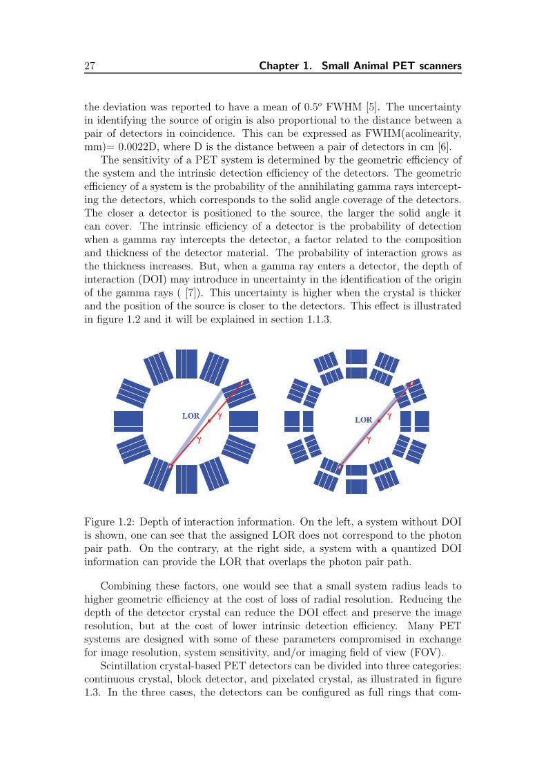
The sensitivity of a PET system is determined by the geometric efficiency ofthe system and the intrinsic detection efficiency of the detectors. The geometricefficiency of a system is the probability of the annihilating gamma rays intercept-ing the detectors, which corresponds to the solid angle coverage of the detectors.The closer a detector is positioned to the source, the larger the solid angle itcan cover. The intrinsic efficiency of a detector is the probability of detectionwhen a gamma ray intercepts the detector, a factor related to the compositionand thickness of the detector material. The probability of interaction grows asthe thickness increases. But, when a gamma ray enters a detector, the depth ofinteraction (DOI) may introduce in uncertainty in the identification of the originof the gamma rays ( [7]). This uncertainty is higher when the crystal is thickerand the position of the source is closer to the detectors. This effect is illustratedin figure 1.2 and it will be explained in section 1.1.3.
Figure 1.2: Depth of interaction information. On the left, a system without DOIis shown, one can see that the assigned LOR does not correspond to the photonpair path. On the contrary, at the right side, a system with a quantized DOIinformation can provide the LOR that overlaps the photon pair path.
Combining these factors, one would see that a small system radius leads tohigher geometric efficiency at the cost of loss of radial resolution. Reducing thedepth of the detector crystal can reduce the DOI effect and preserve the imageresolution, but at the cost of lower intrinsic detection efficiency. Many PETsystems are designed with some of these parameters compromised in exchangefor image resolution, system sensitivity, and/or imaging field of view (FOV).
Scintillation crystal-based PET detectors can be divided into three categories:continuous crystal, block detector, and pixelated crystal, as illustrated in figure1.3. In the three cases, the detectors can be configured as full rings that com-

1.1. Basics of PET 28
pletely surround the patient or as partial rings with rotational motion to obtainthe needed angular sampling.
Figure 1.3: The major crystal-PMT decoding geometry and designs commonlyused in scintillation-crystals-based PET. (a) Continuous crystal read out by anarray of PMTs sensitive to position. (b) Block detector uses pixelated crystalsand PMTs. (c) Full ring of discrete crystals configured as small blocks or largerdetector modules. (d) Partial ring of detector blocks that rotates. (e) Array oflarge detectors, either continuous or discrete crystals. (f) Partial array of largedetector that rotates.
Depending on the design of the scanner, PET data can be acquired in either2D or 3D mode (see figure 1.4). Traditionally, PET data acquisitions were basedon plane-by-plane LOR detection (2D mode). Direct and cross planes originatedfrom LORs detected within the same ring (ring difference 0) or the two adja-cent rings (ring difference ±1), respectively. To shield out-of-plane coincidencephotons that are emitted obliquely, annular septa composed of lead-tungstenseparate the rings. Working in 2D mode, system sensitivity is constrained to adefined value by geometric acquisition conditions and by electronic collimationfixed between adjacent planes. A large increase in sensitivity can be obtainedby collecting all possible LORs; this is possible if the septa are removed. In thisapproach, called 3D mode, the sensitivity is 3-4 times higher than in 2D mode(figure 1.4). However, this gain is associated with an increase in random and

29 Chapter 1. Small Animal PET scanners
scatter coincidences, and the increased counting rate can result in loss of eventsdue to the dead time. To fully take advantage of the 3D mode, faster coincidencedetection is required, along with higher computing power to manage the veryhigh counting rate.
Figure 1.4: Comparison between the sensitivity in 2D (with septa) and 3D (with-out septa) modes [19]
1.1.2 Image Reconstruction
After the two gamma rays have been detected, the next step is to compute,or reconstruct, images from these data. This section is dedicated to explain themain reconstruction algorithms employed in PET.
Acquisition and Organization of Data
A conventional PET scanner counts coincidence events between pairs of detectors.As we have already mentioned, the straight line connecting the inner face centersof two detectors is called a line of response. In the same way, the parallelepipedjoining the two detectors defines the volume of response (VOR) (figure 1.5).In the absence of physical effects such as attenuation, scattered and accidentalcoincidences, and detector efficiency variations, the total number of coincidenceevents detected will be proportional to the total amount of tracer contained inthe hypothetical tube of VOR (shown by the shaded area in figure 1.5b. Becausephoton counting from radioactive decay is a random process, the expectationoperator for each pair of detectors (in this example, detector 1 and 2) is
E{photons detected per second} =∫∫∫
V ORs(x)f(x)dx (1.1)
where s(x) is the detection sensitivity within the tube at x and f(x) is thethree dimensional distribution of radiotracer activity inside the patient.
For the LOR definition, a scanner comprising multiple small detectors wasconsidered. Scanners based on large-area, position-sensitive detectors can bedescribed similarly if viewed as consisting of large number of very small virtualdetectors.

1.1. Basics of PET 30
Figure 1.5: (a) Overall scheme with the line of response (LOR) that joins detector1 and 2. (b) Detail of the sensitive region scanned by the two detectors thatdefines the volume of response (VOR) [19].
LOR Histogram The natural parametrization of PET data uses the twoindices (d1, d2) of the detectors in coincidence or the index of the associated LOR(ld1,d2
). Storing the coincidences for each LOR corresponds to the LOR histogramway of organizing the data. The main advantage of the LOR histogram format isto take full benefit of the nominal spatial resolution of the scanner. The general-ization from 2D to 3D imaging using LOR histogram can be done immediately.But, the natural parametrization is poorly adapted to analytic algorithms. Thisis the principal reason why the raw data are normally interpolated into an alter-native sinogram parametrization (explained in the next section). Another reasonto use the sinogram is that this parametrization is more compact and smallerthan the LOR histogram. When the Nevents << NLOR, there is an approachto reduce data storage and processing time. This format consists of recordingthe LOR index or detector indices of each coincident event in a sequential datastream called a list-mode data set. Additional information such as the time orthe energy of each detected photon can also be stored.
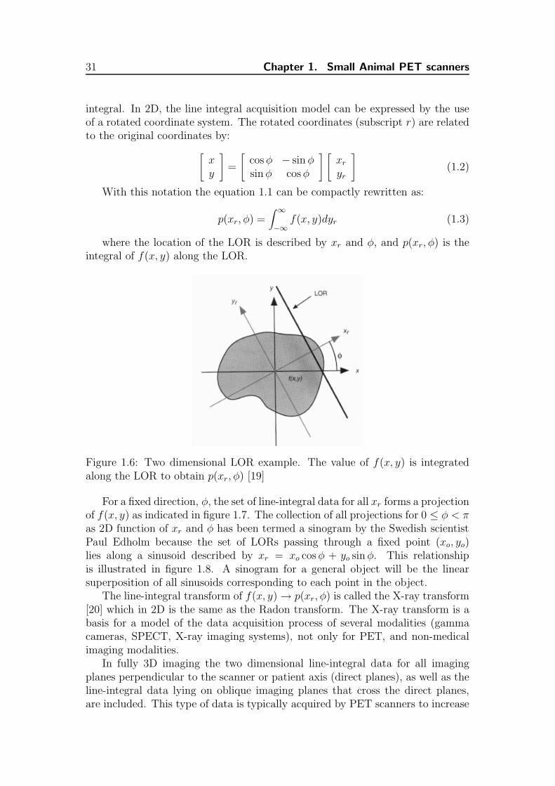
Sinogram For 2D imaging the considered LORs are the ones lying within aspecified imaging plane. The acquired data are collected along a LOR through a2D object f(x, y) as shown in figure 1.6 and the equation 1.1 is written as a line
31 Chapter 1. Small Animal PET scanners
integral. In 2D, the line integral acquisition model can be expressed by the useof a rotated coordinate system. The rotated coordinates (subscript r) are relatedto the original coordinates by:
[
xy
]
=
[
cos φ − sin φsin φ cos φ
] [
xr
yr
]
(1.2)
With this notation the equation 1.1 can be compactly rewritten as:
p(xr, φ) =∫
∞
−∞
f(x, y)dyr (1.3)
where the location of the LOR is described by xr and φ, and p(xr, φ) is theintegral of f(x, y) along the LOR.
Figure 1.6: Two dimensional LOR example. The value of f(x, y) is integratedalong the LOR to obtain p(xr, φ) [19]
For a fixed direction, φ, the set of line-integral data for all xr forms a projectionof f(x, y) as indicated in figure 1.7. The collection of all projections for 0 ≤ φ < πas 2D function of xr and φ has been termed a sinogram by the Swedish scientistPaul Edholm because the set of LORs passing through a fixed point (xo, yo)lies along a sinusoid described by xr = xo cos φ + yo sin φ. This relationshipis illustrated in figure 1.8. A sinogram for a general object will be the linearsuperposition of all sinusoids corresponding to each point in the object.
The line-integral transform of f(x, y) → p(xr, φ) is called the X-ray transform[20] which in 2D is the same as the Radon transform. The X-ray transform is abasis for a model of the data acquisition process of several modalities (gammacameras, SPECT, X-ray imaging systems), not only for PET, and non-medicalimaging modalities.
In fully 3D imaging the two dimensional line-integral data for all imagingplanes perpendicular to the scanner or patient axis (direct planes), as well as theline-integral data lying on oblique imaging planes that cross the direct planes,are included. This type of data is typically acquired by PET scanners to increase

1.1. Basics of PET 32
Figure 1.7: A projection formed from integration along all parallel LOR at anangle φ [19].
Figure 1.8: (a) Relation between LORs passing through a fixed point (xo, yo) and(b) the values of the sinogram p(xr, φ) for a fixed point [19].
sensitivity and lower the statistical noise associated with photon counting, thusimproving the signal-to-noise ratio in the reconstructed image.
For the X-ray transform of a three-dimensional object, four parameters areneeded to parameterize the LOR shown in figure 1.9: Two angles (φ, θ) to de-fine the unit vector zr = (cos φ cos θ, sin φ cos θ, sin θ) parallel to the LOR, and

33 Chapter 1. Small Animal PET scanners
two coordinates (xr, yr) to locate the intersection of the LOR with the planeperpendicular to zr(φ, θ).
Figure 1.9: Parametrization of a 3D LOR for the X-ray transform using a rotatedcoordinate frame [19].
By using the constraint xr · z = 0 and the definition of θ as the co-polar angle,the rotated coordinates are related to the original coordinates by
xyz
=
− sin φ − cos φ sin θ cos φ cos θcos φ − sin φ sin θ sin φ cos θ
0 cos θ sin θ
xr
yr
zr
(1.4)
This choice of rotated coordinates and θ as the co-polar angle is customarybecause the equivalent 2D acquisition, or the direct planes, corresponds to θ = 0.Using the coordinate transform of equation 1.4, the line integral projections alongthe LOR, located by (xr, yr, φ, θ) are easily expressed as:
p(xr, yr, φ, θ) =∫
∞
−∞
f(x, y, z)dzr (1.5)
For a fixed direction, zr(φ, θ), the set of line-integral data for all (xr, yr) formsa two-dimensional projection p(xr, yr, φ, θ) of f(x, y, z), as illustrated in figure1.10. The full projection data set is a four-dimensional function, so the X-raytransform of f(x, y, z) → p(xr, yr, φ, θ) has increased the number of dimensionsby one and this will cause redundancies in the data.
Analytical Methods
Analytic methods typically neglect noise and complicating physical factors in aneffort to obtain frameworks that yield explicit inversion formulas for the recon-struction problem. Analytic methods usually produce solutions that are relativelypractical to compute. The Filtered Back Projection (FBP) method is an exam-ple of this category of image reconstruction approaches referred to as analyticmethods to distinguish them from iterative methods. FBP is a mathematicaltechnique based on an idealized model of PET acquisition that ignores many

1.1. Basics of PET 34
Figure 1.10: Illustration of a 2D line-integral projection p(xr, yr, φ, θ) of a 3Dobject f(x, y, z). The projection is formed from the set of all LORs parallel tox(φ, θ) [19].
significant features of real data. Specifically, FBP assumes that the number ofdetected coincidence events travelling along a particular direction approximatesan integral of the radiotracer distribution along that line, that is, the parallel pro-jection p(xr, yr) defined in figure 1.7. Introducing FBP based on the line-integralmodel means that there are important effects not considered, such as noise, at-tenuation, scatter, and detector size. Suboptimal, but reasonable results can beobtained in practice using FBP, even if attenuation and scatter are not accountedfor1. However, noise must always be accounted for in some way, and this is usu-ally achieved in FBP by smoothing the projections prior to reconstruction or bysmoothing the image afterward.
The Central Section Theorem The central section theorem (also knownas the central slice or projection slice theorem) is the most important relation-ship in analytic image reconstruction. In this section, the derivation of the two-dimensional version will be done first, which is then easily extended to the threedimensional X-ray transform. For all the results presented here, the imaging pro-cess must be shift-invariant, which allows the use of the Fourier transforms. Themeaning of the shift invariance here is that the projections of the scanning of ashifted object are also shifted, but are otherwise identical to the projections of theunshifted object. Shift-invariance is a natural property of ideal two-dimensionalimaging. For fully three-dimensional imaging situation is somewhat more com-plicated.
The definition of the one-dimensional Fourier transform and the inverse trans-form are the starting point of the 2D central section theorem derivation:
F (υx) = F1{f(x)} =∫
∞
−∞
f(x)e−i2πxυxdx
f(x) = F−11 {F (υx)} =
∫
∞
−∞
F (υx)e+i2πxυxdυx (1.6)
where the adopted notation is capital letters for Fourier transformed functions,
1Usually, scatter and attenuation are taken into account before the reconstruction by in-cluding corrections in the sinogram.

35 Chapter 1. Small Animal PET scanners
and, in general, the operator Fn{f(x)} for the n-dimensional Fourier transformof f(x), F−1
n {F (υx)} for the inverse n-dimensional Fourier transform, and υx asthe Fourier space conjugate of x.
The one-dimensional Fourier transform of a projection is given by:
P (υxr, φ) = F1{p(xr, φ)} =
∫
∞
−∞
p(xr, φ)e−i2πxrυxr dxr (1.7)
An important step is the introduction of the definition of p(xr, φ) from equa-tion 1.3,
P (υxr, φ) =
∫
∞
−∞
p(xr, φ)e−i2πxrυxr dxr
=∫
∞
−∞
∫
∞
−∞
f(x, y)e−i2πxrυxr dxrdyr
=∫
∞
−∞
∫
∞
−∞
f(x, y)e−i2π(x cos φ+y sinφ)υxr dxdy
= F (υxrcos φ, υxr
sin φ) (1.8)
where F (υx, υy) = F2{f(x, y)} =∫
∞
−∞
∫
∞
−∞f(x, y)e−i2π(xυx+yυy)dxdy. Because the
Fourier transform is invariant under rotation, it is obtained from the equation1.2:
[
υx
υy
]
=
[
cos φ − sin φsin φ cos φ
] [
υxr
υyr
]
(1.9)
Equation 1.8 can be more concisely expressed using equation 1.9:
P (υxr, φ) = F (υx, υy) |υyr=0 (1.10)
Equation 1.10 is the key to understand tomographic imaging. It shows thatthe Fourier transform of a one-dimensional projection is equivalent to a section,or profile, at the same angle through the center of the two-dimensional Fouriertransform of the object. This is illustrated in figure 1.11. It is known thatany function is uniquely determined by its Fourier transform (that is, it can becomputed via the inverse Fourier transform), the central slice theorem indicatesthat if we know P (υxr
, φ) at angles 0 ≤ φ < π, then it is possible somehow todetermine F (υx, υy) and thus f(x, y).
To derive the central section theorem for the X-ray projection of a 3D object,first the two-dimensional Fourier transform is computed with respect to the firsttwo (linear) variables:
P (υxr, υyr
, φ, θ) =∫
∞
−∞
∫
∞
−∞
p(xr, yr, φ, θ)e−i2π(xrυxr+yrυyr )dxrdyr (1.11)
If F (υx, υy, υz) is the three-dimensional Fourier transform of f(x, y, z)
F (υx, υy, υz) =∫
∞
−∞
∫
∞
−∞
∫
∞
−∞
f(x, y, z)e−i2π(xυx+yυy+zυz)dxdydz (1.12)
1.1. Basics of PET 36
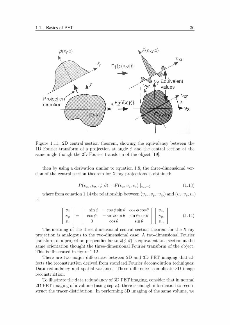
Figure 1.11: 2D central section theorem, showing the equivalency between the1D Fourier transform of a projection at angle φ and the central section at thesame angle though the 2D Fourier transform of the object [19].
then by using a derivation similar to equation 1.8, the three-dimensional ver-sion of the central section theorem for X-ray projections is obtained:
P (υxr, υyr
, φ, θ) = F (υx, υy, υz) |υzr=0 (1.13)
where from equation 1.14 the relationship between (υxr, υyr
, υzr) and (υx, υy, υz)
is
υx
υy
υz
=
− sin φ − cos φ sin θ cos φ cos θcos φ − sin φ sin θ sin φ cos θ
0 cos θ sin θ
υxr
υyr
υzr
(1.14)
The meaning of the three-dimensional central section theorem for the X-rayprojection is analogous to the two-dimensional case: A two-dimensional Fouriertransform of a projection perpendicular to z(φ, θ) is equivalent to a section at thesame orientation thought the three-dimensional Fourier transform of the object.This is illustrated in figure 1.12.
There are two major differences between 2D and 3D PET imaging that af-fects the reconstruction derived from standard Fourier deconvolution techniques:Data redundancy and spatial variance. These differences complicate 3D imagereconstruction.
To illustrate the data redundancy of 3D PET imaging, consider that in normal2D PET imaging of a volume (using septa), there is enough information to recon-struct the tracer distribution. In performing 3D imaging of the same volume, we

37 Chapter 1. Small Animal PET scanners
Figure 1.12: 3D central section theorem for X-ray transforms, showing the equiv-alency between the 2D Fourier transform of a projection in direction z(φ, θ) andthe central section at the same angle though the 3D Fourier transform of theobject [19].
collect a super-set of the 2D data, therefore the additional data must consist ofredundant information. The key point of 3D PET imaging is that the collectionof this redundant information along the additional LORs, if used properly, canimprove the image signal-to-noise ratio by reducing the statistical noise.
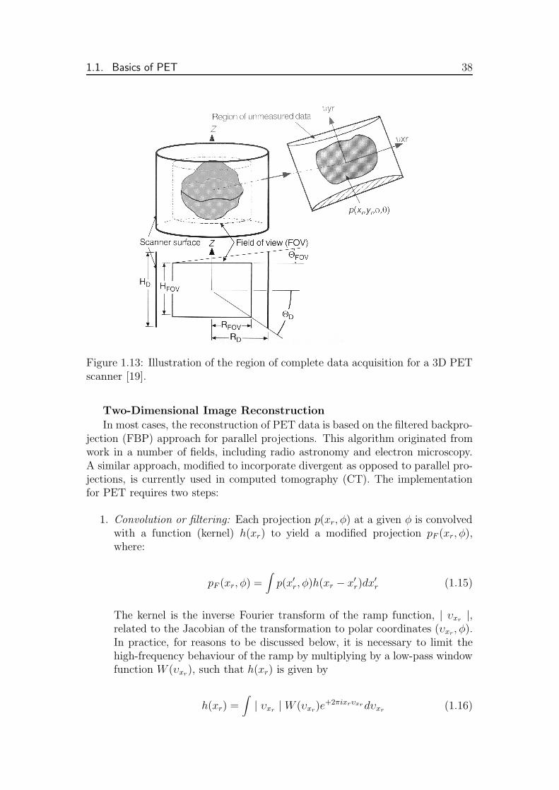
The shift variance of 3D PET can be understood by considering figure 1.13,which illustrates how a projection is truncated due to the finite axial extent ofthe scanner. To develop the theory and algorithms required to reconstruct thetracer distribution, it is necessary to assume that p(xr, yr, φ, θ) is known for all(xr, yr). In other words, it is necessary to measure all the LORs parallel toz = (cos φ cos θ, sin φ cos θ, sin θ (defined in figure 1.9) and crossing the regionDf , where Df is the support of the object, that is, where f(x) 6= 0. If theprojections are not truncated, they are said to be complete. If all projectionswere complete, the sensitivity of the scanner would be independent of the positionin the field-of-view and the reconstruction problem would be stationary (shift-invariant) and could be solved using standard Fourier deconvolution techniques.The 2D reconstruction problem, with a multiring scanner operated with the septaextended, is shift-invariant provided the small effects such as the parallax error areneglected or corrected. In contrast, the 3D problem is not shift-invariant becausethe solid angle subtended by the scanner decreases when one moves away fromthe center of the field-of-view along the scanner axis. Truncation increases thecomplexity of the reconstruction because filtered-backprojection, being based onFourier deconvolution, cannot be applied to incomplete data. For the impracticalcase of a nontruncated spherical scanner (ΘD = π/2), the scanner response wouldbe spatially invariant, although the issue of data redundancy would remain.
1.1. Basics of PET 38
Figure 1.13: Illustration of the region of complete data acquisition for a 3D PETscanner [19].
Two-Dimensional Image Reconstruction
In most cases, the reconstruction of PET data is based on the filtered backpro-jection (FBP) approach for parallel projections. This algorithm originated fromwork in a number of fields, including radio astronomy and electron microscopy.A similar approach, modified to incorporate divergent as opposed to parallel pro-jections, is currently used in computed tomography (CT). The implementationfor PET requires two steps:
1. Convolution or filtering: Each projection p(xr, φ) at a given φ is convolvedwith a function (kernel) h(xr) to yield a modified projection pF (xr, φ),where:
pF (xr, φ) =∫
p(x′
r, φ)h(xr − x′
r)dx′
r (1.15)
The kernel is the inverse Fourier transform of the ramp function, | υxr|,
related to the Jacobian of the transformation to polar coordinates (υxr, φ).
In practice, for reasons to be discussed below, it is necessary to limit thehigh-frequency behaviour of the ramp by multiplying by a low-pass windowfunction W (υxr
), such that h(xr) is given by
h(xr) =∫
| υxr| W (υxr
)e+2πixrυxr dυxr(1.16)

39 Chapter 1. Small Animal PET scanners
The convolution may be equivalently performed in Fourier space where theconvolution operation reduces to a simple multiplication ( [21]). Thus:
pF (xr, φ) =∫
∞
−∞
PF (υxr, φ)e+i2πxrυxr dυxr
PF (υxr, φ) = | υxr
| W (υxr)∫
∞
−∞
p(xr, φ)e−i2πxrυxr dxr (1.17)
The Fourier transform of the convolving function h(xr), i.e. | υxr| W (υxr
),is called a filter, and hence equation 1.17 is referred to as the filtering stepand pF (xr, φ) as filtered projections.
2. Backprojection:
The reconstruction fR(x, y) of the tracer function f(x, y) is formed from thefiltered projections by redistributing the filtered projection value pF (xr, φ)uniformly along the straight line (xr, φ):
fR(x, y) =∫ π
0pF (x cos φ + y sin φ, φ)dφ (1.18)
This operation is called backprojection since formally it is the reverse of theprojection process, the value of fR(x, y) at the point (x, y) being obtainedby summing the contributions.
In practice, PET images are reconstructed from sinograms using discretizedversions of equations 1.17 and 1.18. The discretization of these expressions canbe found in [22].
An important feature of the kernel h(xr) that appears in equation 1.15 is itsdependence on the distance xr−x′
r rather than on the separate coordinates xr andx′
r. This property relates to the fact that the kernel is shift-invariant, meaningthat all projections values are filetered using the same kernel. Any translation ofthe tracer distribution f(x, y) results in a corresponding translation of the projec-tion data p(xr, φ), without modifying the form of equation 1.3. The simple formof equation 1.17 is then a direct consequence of the shift-invariance of h(xr). Inpractice, however, shift-invariance is only approximately satisfied due to the sensi-tivity variations within a LOR and to differing LOR cross sections. Nevertheless,these variations are, in general, small, and shift-invariance is a reasonable approx-imation for the reconstruction of direct and cross plane sinograms. Unfortunately,shift-invariance is not satisfied in the case of three-dimensional acquisition, butthis will be discussed in the next section.
Three-Dimensional Image ReconstructionFor a tomograph comprising multiple rings of detectors, a 3D image of the
tracer distribution f(x, y, z) can be built up by stacking a set of independent 2Dslices. Each slice is reconstructed independently of the adjacent slices. However,this procedure is no longer possible when coincidences are acquired between all

1.1. Basics of PET 40
ring of detectors. A full 3D acquisition necessitates a full 3D reconstructionalgorithm in order to correctly incorporate the sinograms for the oblique LORs.The problem, therefore, is to recover the tracer concentration f(x, y, z) from theline integrals defined by equation 1.5 modified to the 3D case.
Reconstruction of the tracer distribution f(x, y, z) from the integrals p(xr, yr, φ, θ)is therefore a problem of inverting the X-ray transform in the three dimensions.Unlike the 2D case, in the 3D the Radon transform is not equivalent to the X-ray transform, equation 1.5. Whether or not the inversion is possible dependsupon the set of line integrals which have been measured by the tomograph. As-sume initially that the line integrals are measured for a limited set of directions0 ≤ φ < π and −Θc ≤ θ < Θc, but for all coordinate pairs (xr, yr) for which thestraight line (xr, yr, φ, θ) intersects the 3D field of view. This means that, whilenot all possible parallel projections are measured because of the limited range ofθ, those projections which are measured are complete.
Although not all possible line integrals through the field of view are available(since | θ |< Θc < π), the solution of the equation 1.5 is nevertheless unique, andcan be obtained by straightforward generalisation of equations 1.15 to 1.18 above
1. Convolution or filtering : Each 2D parallel projection is convolved with akernel h(xr, yr, θ), independent of φ, to give the filtered projection pF (xr, yr, φ, θ):
pF (xr, yr, φ, θ) =∫ ∫
p(x′
r, y′
r, φ, θ)h(xr − x′
r, yr − y′
r, θ)dx′
rdy′
r (1.19)
As for the 2D case, this filtering operation may be more efficiently performedusing the Fourier convolution theorem than by implementing equation 1.19directly.
2. Backprojection: The 2D filtered projections are backprojected by redis-tributing the values pF (xr, yr, φ, θ) uniformly along the line (xr, yr, φ, θ) soas to form the reconstructed image:
fR(xr, yr, φ, θ) =∫ π
0dφ
∫ Θ
−Θcos θpF (xr, yr, φ, θ)dθ (1.20)
with xr = −x sin φ + y cos φ and yr = −x cos φ sin θ − y sin φ sin θ + z cos θ.
The expressions in equation 1.20 for the projection coordinates (xr, yr) en-sure that the line (xr, yr, φ, θ) passes through the point (x, y, z). Thus, asin the 2D case, the reconstructed value fR(x, y, z) at the point (x, y, z) isobtained by summing the contributions from all the backprojection lines(xr, yr, φ, θ) which pass through (x, y, z). In analogy to the equation 1.17,the convolution kernel h(xr, yr, θ) may be expressed as the Fourier transformof a filter function H(υxr
, υyr, θ) multiplied by a low-pass window function
W (υxr, υyr
):

41 Chapter 1. Small Animal PET scanners
h(xr, yr, θ) =∫ ∫
H(υxr, υyr
, θ)W (υxr, υyr
)e2πi(xrυxr +yrυyr )dυxrdυyr
(1.21)
where (υxr, υyr
) are frequency space cartesian coordinates corresponding tothe projection coordinates (xr, yr). Equivalently, polar coordinates (ρ, α)can be defined by:
υxr= ρ cos α, υyr
= ρ sin α, with ρ2 = υ2xr
+ υ2yr
(1.22)
An appropriate filter function H(υxr, υyr
, θ) was published by Colsher [23]expressed in frequency space polar coordinates on the projection plane as:
H(ρ cos α, ρ sinα, θ) =πρ
arcsin sinΘZ
if Z ≥ sin Θ
= 2ρ if Z < sin Θ (1.23)
where Z =√
cos2 α + sin2 α sin2 θ and | θ |≤ Θc.
As in the 2D (equation 1.16), the filter function is proportional to the mod-ulus of the frequency, ρ. In addition, since equation 1.19 is a convolutionequation, the measured data set p(xr, yr, φ, θ) is required to be shift invari-ant.
Unfortunately, in practice, the 3D data set acquired by a multi-ring PETtomograph does not satisfy the conditions for shift-invariance. This has beenexplained in section 1.1.2, page 34. Under these conditions, the filtered backpro-jection algorithm cannot be applied to reconstruct the data.
If, however, some angle Θc can be defined such that, for | θ |≤ Θc, say, thecorresponding parallel projections are completely measured, then the algorithmcould successfully be applied to a subset of the 3D data, rejecting those partially-measured projections with angles | θ |> Θc ( [23], [24]). Indeed, this was thecondition under which the algorithm was originally derived earlier in this section,that all projections for | θ |≤ Θc were completely measured. From figure 1.14, itcan be seen that, as the tracer distribution extends axially from the centre, theangle Θc for which all projections are completely measured becomes progressivelysmaller. Finally, when the tracer distribution covers the full axial extent of thetomograph, Θc ≈ 0.
One of the simplest solutions to the problem of how to incorporate the obliqueLORs from a multi-ring tomograph into a 3D reconstruction using filtered back-projection is based on the following idea ( [25], [26], [27]): since the projectionswhich give rise to shift-variance are incomplete, and it is desired to include them ina filtered backprojection reconstruction, why not complete these projections be-fore including them. Then the reconstruction will again involve only completely-measured projections and can be performed, as outlined earlier in this section,by 3D filtered backprojection.
1.1. Basics of PET 42
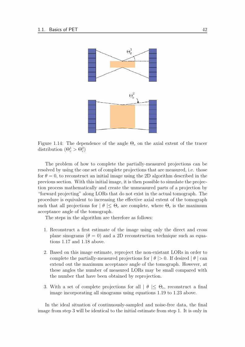
Figure 1.14: The dependence of the angle Θc on the axial extent of the tracerdistribution (Θ1
c > Θ2c)
The problem of how to complete the partially-measured projections can beresolved by using the one set of complete projections that are measured, i.e. thosefor θ = 0, to reconstruct an initial image using the 2D algorithm described in theprevious section. With this initial image, it is then possible to simulate the projec-tion process mathematically and create the unmeasured parts of a projection by“forward projecting” along LORs that do not exist in the actual tomograph. Theprocedure is equivalent to increasing the effective axial extent of the tomographsuch that all projections for | θ |≤ Θc are complete, where Θc is the maximumacceptance angle of the tomograph.
The steps in the algorithm are therefore as follows:
1. Reconstruct a first estimate of the image using only the direct and crossplane sinograms (θ = 0) and a 2D reconstruction technique such as equa-tions 1.17 and 1.18 above.
2. Based on this image estimate, reproject the non-existant LORs in order tocomplete the partially-measured projections for | θ |> 0. If desired | θ | canextend out the maximum acceptance angle of the tomograph. However, atthese angles the number of measured LORs may be small compared withthe number that have been obtained by reprojection.
3. With a set of complete projections for all | θ |≤ Θc, reconstruct a finalimage incorporating all sinograms using equations 1.19 to 1.23 above.
In the ideal situation of continuously-sampled and noise-free data, the finalimage from step 3 will be identical to the initial estimate from step 1. It is only in

43 Chapter 1. Small Animal PET scanners
the presence of statistical noise that the incorporation of the additional obliqueLORs serves to improve the signal to noise of the final 3D reconstruction.
Iterative Methods
While the analytic approaches typically result in fast reconstruction algorithms,accuracy of the reconstructed images is limited by the approximations implicitin the linear-integral model on which the reconstruction formulae are based. Incontrast to the analytical methods, an iterative model-based approach can simplymodel the mapping from source to detector without requiring explicit line-integralor other models. The simplest iterative methods use on-the-fly computation offorward and backprojection with the same linear-interpolation-based method asis commonly used in FBP. A more flexible approach, which allows more accu-rate modelling of the physical detection process, is to precompute and store theprojection matrices that define this mapping.
Iterative algorithms are based on the attempt to maximize or minimize a tar-get function determined by the particular algorithm used. The target is reachedthrough several analytic processes called iterations. A major advantage of thistype of algorithm is the possibility of incorporating different a priori information,such as noise component, attenuation, or characteristics of detector nonunifor-mity, for more accurate image reconstruction; however, it must be pointed outthat inclusion of additional parameters means increase in processing times. De-pending on the method, different numbers of iterations are required to reach thetarget function, keeping in mind that too many iterations can easily lead to noiseamplification with image quality deterioration. For this reason, it is importantto perform an accurate evaluation of the number of iterations needed to obtainthe best image quality.
Data and Image ModelThe PET reconstruction problem1 can be formulated as the following estima-
tion problem: “Find the object distribution f , given (1) a set of measurements d,(2) information (in the form of a matrix P) about the imaging system that pro-duced the measurements, and, possibly, (3) a statistical description of the dataand (4) a statistical description of the object (figure 1.15)”.
Indeed, under the assumption that the imaging process is linear, the PETreconstruction problem is like any linear inverse problem of the following form:
di =∫
RDf(x)pi(x)dx i = 1, ..., I (1.24)
where x is a vector denoting spatial coordinates in the image domain, di
represents the ith measurement, and pi(x) is the response of the ith measurementto a source at x. In 2D slice imaging, D = 2 and x = (x, y); in 3D imaging, D = 3and x = (x, y, z). The point spread function (PSF) pi(x) can represent the effectsof attenuation and all linear sources of blur. A good example of how various effectscan be incorporated in the PSF can be found in [28].
1like any emission tomography (ET) problem
1.1. Basics of PET 44
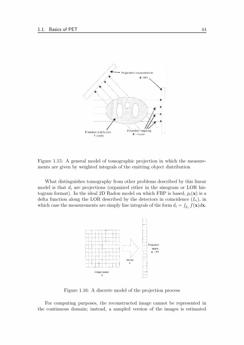
Figure 1.15: A general model of tomographic projection in which the measure-ments are given by weighted integrals of the emitting object distribution
What distinguishes tomography from other problems described by this linearmodel is that di are projections (organized either in the sinogram or LOR his-togram format). In the ideal 2D Radon model on which FBP is based, pi(x) is adelta function along the LOR described by the detectors in coincidence (Li), inwhich case the measurements are simply line integrals of the form di =
∫
Lif(x)dx.
Figure 1.16: A discrete model of the projection process
For computing purposes, the reconstructed image cannot be represented inthe continuous domain; instead, a sampled version of the images is estimated

45 Chapter 1. Small Animal PET scanners
and described in a discrete domain by column vector f (figure 1.16). Thus, eachmeasurement in equation 1.24 can be approximated by the following system oflinear equations:
di = pTi f i = 1, ..., I (1.25)
which can be summarized by a single matrix equation as follows:
d = Pf (1.26)
Here, pi is the ith row of P, and each element of f , denoted by fj, j = 1, ..., J ,represents one pixel in the image space. In this general notation, f may representeither a 2D slice image or a 3D volume image, and complicated imaging systemscan be readily represented within this approach by appropriate definition of P.The word pixel refers to elements of the image domain, although it should beunderstood to encompass the term voxel, which is an element of a volume image.Note that the measurement or projection space is also discrete, with the projectiondata represented by the vector d. The elements of d are referred to here asprojection bins or simply bins, and every projection measurement is representedby one bin. This bin can belong to the LOR histogram or to the sinogram,depending on the organization of data.
Considering the randomness in the projection data, due to the variabilityinherent in the photon-counting process used in PET, equation 1.26 should bewritten as:
E[d] = Pf (1.27)
where E[] denotes the expected value.Photon emissions are known to obey the Poisson distribution, and photo de-
tections also obey the Poisson distribution, provided that detector dead time canbe neglected and that no correction factors have been applied to the data. Inthis case, the number of events detected in the projection bins are independentof one another. Thus, the probability law for d is given by:
p(d; f) =I
∏
i=1
ddi
i e−di
di!(1.28)
where di is the ith element of E[d] = Pf :
di =J
∑
j=1
pijfj (1.29)
Although is not exact for real imaging systems, the Poisson model is a gooddescription of raw PET data and is the most commonly used model in the PETfield. However, other probability models are often used. For example, when aPET imaging system internally corrects for random coincidences by subtractingan estimated randoms contribution, the statistics can be described by a shiftedPoisson model [29]. Gaussian models, which are used in cases in which the mean

1.1. Basics of PET 46
number of events is reasonably high, are also often used because of their practicaladvantages.
In writing equation 1.24, it was ignored the fact that the activity distributionin the patient is actually a function of time. This fact is not considered in astatic PET study, in which all the counts measured during the imaging sessionare summed together and used to produce a single static image of the patient.In this case, f(x) in equation 1.24 should be interpreted as the time averageof the spatiotemporal activity distribution f(x, t). Whereas the static studyis concerned only with the spatial distribution of the tracer, gated studies anddynamic studies also measure temporal variations of the tracer concentration. In aPET study, there are two types of temporal variations of interest: (1) fluctuationscaused by physiological interactions of the tracer with the body and (2) cardiacmotion, which helps assess whether the heart is functioning normally. Othertemporal variations, including respiratory motion, voluntary patient motion, andthe steady decline of activity associated with radioactive decay, are effects to becorrected for, if possible. For time-sequence imaging, as in the case of dynamicor gated studies, the imaging model may be expressed as follows:
dik =1
τk
∫
ll
dt∫
RD+1
dxf(x, t)pi(x, t) i = 1, ..., I; k = 1, ..., K (1.30)
where lk is the time interval of duration τk during which the kth frame of thedata is acquired.
System Matrix In the equation 1.26, P is a I × J matrix called systemmatrix, which describes the imaging process, and can include attenuation andany linear blurring mechanisms. Each element of P (denoted by pij) representsthe mean contribution of pixel j in the object to bin i in the projections. It isin the specification of P that the model of the projection process can become assimple or as complex as we require because the intensity of a projection bin is aweighted sum of intensities of the image pixels. To represent the Radon case, thematrix elements are defined so that a projection bin receives contributions onlyfrom pixels that are intersected by a given line and the contributions of pixels thatdo not intersect the line are set to zero. The linear model can also represent a morerealistic case wherein a projection bin receives contributions from many pixels,each weighted according to the relative sensitivity of the projection bin to eachpixel. These contributions are affected by physical factors such as attenuation,detector response, and scatter and can be estimated from knowledge of the systemdesign and measurement of the patient attenuation distribution. There are severalmethods to build the system matrix and they will be summarized in chapter 3.This chapter is dedicated to the creation of the system matrix for a dedicatedsmall animal PET scanner.
General Components and Structure of Iterative AlgorithmAny method for image reconstruction is composed of two related but distinct
components. The first component, which is called criterion, is the statistical basisor governing principle for determining which image is to be considered as the best

47 Chapter 1. Small Animal PET scanners
estimate of the true image. The second component, which it is called algorithm,is the computational technique used to find the solution specified by the criterion.In other words, the criterion is a strategy, and the algorithm is a set of practicalsteps to implement that strategy.
Most iterative reconstruction algorithms fit the general model shown in figure1.17. The process is begun with some initial estimate f0 of the pixel intensityvalues in the image. A projection step is applied to the current image estimatefn, which yields a set of projection values dn that would be expected if fn wherethe true image. The predicted projections dn are then compared with the actualmeasured data d to create a set of projection-space error values ed. These aremapped back to the image space through a back-projection operation to produceimage-space error values ef that are used to update the image estimate, whichbecomes the new estimate fn+1. This process is repeated again and again until theiteration stops automatically or is terminated by the user. Each of the repetitionis called iteration. At the conclusion of the process, the current image estimateis considered to be the final solution.
Figure 1.17: Flowchart of a generic iterative reconstruction algorithm
The details of the projection, comparison, backprojection, and update stepshave not been specified because, principally, it is in these steps where the indi-vidual reconstruction algorithms differ. The power of iterative methods lies inthe use of this feedback loop to improve the reconstructed image, in comparisonto the FBP that uses only the backprojection portion of the loop and there is nofeedback about the image estimate.
The Maximum-Likelihood Expectation-Maximization AlgorithmNumerous iterative algorithms are present in literature, some based on method-
ologies of numeric linear algebra and others based on statistical approaches.To the latter class belongs the maximum-likelihood expectation maximization(MLEM), which is the standard algorithm and is able to estimate accuratelyradiotracer distribution. The MLEM is based on the maximization of the loga-
1.1. Basics of PET 48
rithm of a Poisson-likelihood target function [17], this is the maximum-likelihood(ML) criterion, and the method uses the expectation maximization algorithm(EM). The attempt is to obtain a reconstructed slice whose forward projectiongenerates a projection dataset almost equal to the original one. When appliedto the PET reconstruction problem (or indeed to any linear inversion problemwith Poisson noise), the MLEM framework yields the following simple iterativeequation, which is easy to implement and understand:
fm+1j =
fmj
∑Ii=1 pij
I∑
i=1
pij
di∑J
b=1 pibfb
, (1.31)
The main feature of its reconstruction algorithm is to update the image duringeach iteration by using a multiplicative factor assessed as the ratio between theoriginal acquired projections and the newly estimated ones. Advantages of thisiterative method are the fact that all reconstructed values will be positive becausea nonnegativity condition is imposed on the original data, the count preservationat each iteration, and the algorithm is simple to implement by a computer. Themain disadvantage is the large number of iterations required to converge to anoptimal solution and then the long processing times (one or two orders of mag-nitude more processing time than FBP), hampering its applicability in clinicalroutine. Another shortcoming of MLEM algorithm is that it provides very noisyreconstructed images. As the iteration process advances, the noise in the im-age increases. However, one should keep in mind that the MLEM algorithm canperform much better than FBP.
To overcome the problem of slow convergence rate, the ordered-subsets ex-pectation maximization (OSEM) algorithm was proposed in 1994, which is nowthe most widely used iterative reconstruction method in whole-body PET imag-ing [18].
The OSEM is a modified version of MLEM (the target is still the maximizationof the log-likelihood function) with the main difference being that projections aregrouped into subsets having projections uniformly distributed around the volumeto be imaged. Within each iteration the target function is updated as manytimes as the number of subsets, proportionally accelerating convergence. Anoptimization of subsets and iterations number is required when the method isapplied to real, noisy data, because the algorithm can cycle without convergingto the MLEM function.
Finally, a few words about spatial resolution achieved with the different re-construction algorithms. Shift invariant linear imaging systems are often charac-terized by their PSF. Noiseless data from a point source will produce an image ofthe PSF so that the measurement of the full-width-at-half-maximum (FWHM) ofthe PSF is a measure of system resolution. This measurement is useful for imagesreconstructed using filtered backprojection since the reconstruction procedure islinear. For non-linear estimators, such a ML, the PSF is spatially variant andobject dependent. Therefore, the PSF can only be examined locally and with aspecific object [30].

49 Chapter 1. Small Animal PET scanners
1.1.3 Image Degradation and Compensation
Parallax Error
The parallax error results from the uncertainty of the depth of interaction of thegamma rays in the crystal and affects the PET image resolution. The gammarays travel some (unknown) distance in the crystal (or adjacent crystals) beforean interaction occurs. If the source is located near the center of the FOV, gammarays enter the two detectors at near-normal angle. The depth of interaction doesnot affect the positioning accuracy of the coincidence LOR defined by the twodetectors. When the source is off-center, the gamma rays enter the detectors atan oblique angle that increases with the radial offset of the source. Dependingon the DOI, the detector in which the interaction occurs may not be the samedetector that initially intercepts the gamma ray. If the design of the detectorcan identify the depth of interaction, the coincidence LOR can be accuratelydefined. However, if the detector is not capable of providing DOI informationand only assumes a predetermined depth as the interaction point, there is afinite probability that the coincidence LOR is mispositioned. The loss of radialresolution can be seen in figure 1.2 as the source is moved away from the centerof the FOV. This parallax error caused by the DOI effect depends on four factors:(a) the radius of the system, (b) the total depth of the detector, (c) the radialoffset of the source, and (d) the detector material.
Scatter
When a positron annihilates in the body, there is a reasonable chance that oneor both of the annihilation photons will scatter in the body (object scatter) or inthe detector itself (detector scatter). At the energy of the annihilation photons(511 keV), the most likely type of interaction is Compton scattering in which thephoton transfers some of its energy to loosely bound electrons and deviates formits initial path [31]. Since the coincidence LOR formed after one or both photonsundergo Compton scattering is no longer colinear with the site of annihilation (fig-ure 1.1), such events degrade the PET measurement. Scatter results in generallydiffuse background counts in reconstructed PET images, reducing contrast anddistorting the relationship between image intensity and activity concentration.
The proportion of accepted coincidences which have undergone Compton scat-tering is referred to as the scatter fraction and its magnitude depends on severalfactors, including the size and density of the scattering medium, the geometryof the PET scanner and the width of the energy-acceptance window (which ismainly determined by the energy resolution of the detectors). The scatter frac-tion typically ranges from about 15% in a ring tomograph with slice-definingsepta (2D mode) to 40% or more for the same tomograph operated without septa(3D mode), [57], [58].
Although the underlying physics describing Compton scattering of annihila-tion photons is reasonably complex, there are several characteristics of the resul-

1.1. Basics of PET 50
tant LORs which can be exploited to estimate their distribution and potentiallycorrect the measured data. For example:
1. LORs recorded outside the object boundary can only be explained by scat-ter in the object (assuming that randoms have been subtracted) since LORsarising from unscattered trues must be colinear with the point of annihila-tion.
2. The scatter distribution is very broad and relatively featureless.
3. The portion of the energy spectrum below the photopeak has a large con-tribution from scatter events.
4. Scattered coincidences that fall within the photopeak are mainly due tophotons that have only scattered once.
These various characteristics have given rise to a wide variety of approachesfor estimating and correcting scattered coincidences in PET data. They can bebroadly divided into four categories: empirical approaches [61], methods basedon two or more energy windows [62] [63], convolution-deconvolution methods [59][60], and model-based algorithms [64] [65]. The explanation of these approachesare out of the scope of this work and the author refer to the bibliography.
Random Coincidences
As it has been already explained, a PET acquisition consists in the simultaneousdetection of two 511 keV photons. Considering the time of flight of the photons,the scintillation time and the processing electronics, it is necessary to accept theevents with a time difference. As a consequence, two uncorrelated single detectionevents occurring sufficiently close together in time can be mistakenly identifiedas a true coincidence event arising from one annihilation. These are the randomcoincidences, also known as “accidental” or “chance” coincidences, they are theprimary source of background noise and image distortion in a PET scanner.
As it was already mentioned, the fully 3D acquisition also leads to an increasein the axial extent of the random coincidence event FOV relative to the truecoincidence FOV, which is even more significant for scanners with larger radialFOVs relative to the end-shield aperture.
Prior to correct for this effect, it is necessary to estimate their contribution.In the following paragraphs, some methods to estimate the random coincidencesare presented.
Delayed-Window (DW) Method. In this method, random coincidencesare estimated by measuring coincidences within a second time window that isdelayed in time (delayed window). The delayed window has the same widthas the time coincidence window and is opened after a time interval ∆T , whichis much larger than its width. Therefore, it can be assumed that the singlesfound in the delayed window are uncorrelated with those in the prompt window.
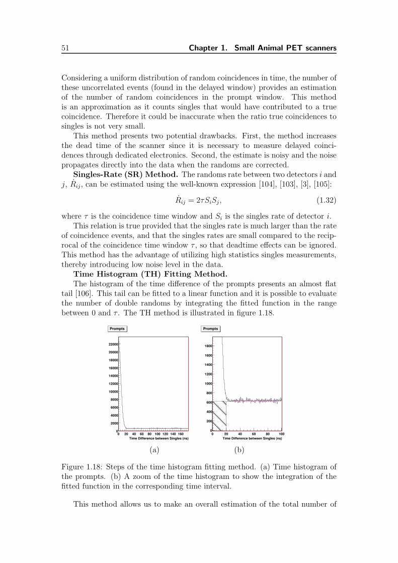
51 Chapter 1. Small Animal PET scanners
Considering a uniform distribution of random coincidences in time, the number ofthese uncorrelated events (found in the delayed window) provides an estimationof the number of random coincidences in the prompt window. This methodis an approximation as it counts singles that would have contributed to a truecoincidence. Therefore it could be inaccurate when the ratio true coincidences tosingles is not very small.
This method presents two potential drawbacks. First, the method increasesthe dead time of the scanner since it is necessary to measure delayed coinci-dences through dedicated electronics. Second, the estimate is noisy and the noisepropagates directly into the data when the randoms are corrected.
Singles-Rate (SR) Method. The randoms rate between two detectors i andj, Rij , can be estimated using the well-known expression [104], [103], [3], [105]:
Rij = 2τSiSj , (1.32)
where τ is the coincidence time window and Si is the singles rate of detector i.This relation is true provided that the singles rate is much larger than the rate
of coincidence events, and that the singles rates are small compared to the recip-rocal of the coincidence time window τ , so that deadtime effects can be ignored.This method has the advantage of utilizing high statistics singles measurements,thereby introducing low noise level in the data.
Time Histogram (TH) Fitting Method.The histogram of the time difference of the prompts presents an almost flat
tail [106]. This tail can be fitted to a linear function and it is possible to evaluatethe number of double randoms by integrating the fitted function in the rangebetween 0 and τ . The TH method is illustrated in figure 1.18.
(a) (b)
Figure 1.18: Steps of the time histogram fitting method. (a) Time histogram ofthe prompts. (b) A zoom of the time histogram to show the integration of thefitted function in the corresponding time interval.
This method allows us to make an overall estimation of the total number of
1.1. Basics of PET 52
randoms in the acquisition, but it is not useful for obtaining a random estimatefor each LOR or element of the sinogram since there are not enough coincidenceevents in a single LOR or element of the sinogram for a useful histogram.
Normalization
The lines of response in a PET dataset have different sensitivities for a vari-ety of reasons including variations in detector efficiency, solid angle subtended,summation of neighboring data elements... Information on these variations isrequired for the reconstruction of quantitative and artifact-free images – indeed,some algorithms require that these variations are removed prior to reconstruc-tion. The process of correcting for these effects is known as normalization, andthe individual correction factors for each LOR are referred to as normalizationcoefficients.
In general, the causes of sensitivity variations are summarized in the following:
• Summing of adjacent data elements. It is common practice to sum adjacentdata elements in order to simplify reconstruction or to reduce the size of thedataset. This effect is fairly simple to account for, since the degree of sum-ming is always known. However, it can complicate the process of correctingthe other effects if the summing is performed prior to normalization.
• Rotational sampling. In a rotating system, LORs at the edge of the fieldof view are sampled just once per half-rotation, while those near the centerare sampled many times. As a result, sensitivity falls as radius increases.
• Detector efficiency variations. In a detector system, detector elements varyin efficiency because of the position of the element in the block, physicalvariations in the crystal and light guides, and variations in the gains of thephotomultiplier tubes. These variations result in substantial high-frequencynon-uniformities in the raw data.
• Geometric and solid angle effects. Figure 1.19 shows that in a system withsegmented detectors, the volumes that cover the detectors in coincidenceclose to the edge of the field of view are narrower and more closely spacedthan those at the center. The narrowing of the VORs yields in a tighter ac-ceptance angle and in reduced sensitivity, although in the transaxial planethis effect is partially compensated for by the fact that the separation be-tween opposing detectors is less towards the edge of the FOV, so that theacceptance angle increases when the LORs are closer to the FOV border.The narrowing of the VORs also results in reduced sampling distance. How-ever, this effect is easily describable analytically and can be corrected forat reconstruction time, this process is known as “arc-correction”. Arc cor-rection may not be an issue for systems that employ continuous detectors.
An effect that is relevant for systems employing either continuous or discretedetectors, and that is not so easy to describe analytically, is related to the

53 Chapter 1. Small Animal PET scanners
angle of incidence of the LOR at the detector face. A photon entering acrystal at angle will usually have more material in its path than one enteringnormally, thus having an increased probability of interaction. In the case ofa ring scanner, this results in measurable changes in sensitivity as the radialposition of the LOR is increased and is known as the radial, or tansaxial,geometric effect.
• Time window alignment. In order for coincidence detection to work ef-ficiently, timing signals from each detector must be accurately synchro-nized. Asynchronicity between detector pairs results in an offset and effec-tive shortening of the time window for true and scatter (but not random)coincidences. This, in turn, results in variations in the sensitivity to trueand scatter coincidences.
• Structural alignment. In a ring tomograph, the accuracy with which the de-tectors are aligned in the gantry can affect LOR efficiency. Such variationswill manifest in different ways depending on the exact design of the tomo-graph, the detectors, and any casing in which the detectors are contained.
Figure 1.19: (a) The VORs are narrower as the radial distance increases. (b) Atthe edges of the FOV, the LORs are more closely spaced compared to the onesat the center.
The simplest approach to normalization is to illuminate all possible LORswith a planar or rotating line positron source (usually 68Ge). Once an analyticalcorrection for non-uniform radial illumination has been applied, the normalizationcoefficients are assumed to be proportional to the inverse of the counts in eachLOR. This process is known as “direct normalization” [66]. Problems with thisapproach include:
1. In order to obtain adequate statistical quality in the normalization dataset,scan times are long; typically several hours.
2. The used sources must have a very uniform activity concentration or theresultant normalization coefficients will be biased.

1.1. Basics of PET 54
To reduce normalization scan times, variance-reduction techniques can beapplied. However, in order to implement these, the normalization coefficientsmust be factored into a series of components, each reflecting a particular sourceof sensitivity variation (described above). This approach is known as component-based model for normalization. A drawback of this approach is that the accuracyof the normalization is dependent on the accuracy of the model used to describethe tomograph. However, it has the advantage that a more intelligent treatmentof the different properties of scattered and true coincidences is possible, whichcan be very helpful in 3D imaging.
Although the plane sources have been suggested as the ideal geometry forPET normalization [131], [134], the sources which have been used for normalizing3D PET systems are:
• Plane source using 68Ge in [134]
• Uniform 20 cm diameter cylinder, usually containing 68Ge in [135]
• 68Ge transmission scanning rod sources in 2D used in [133]
• 68Ge transmission scanning rod sources in 3D used in [136]
• a line source of 68Ge which oscillates across the transaxial field of view,emulating a plane source [138]
When the normalizaton is acquired with transmission ring or rod sources,one concern is that the location of the sources relative to the detectors are verydifferent to that when imaging an object in the centre of the tomograph (thisapplied to both 2D and 3D acquisitions). But, little difference is observed betweenrod sources and a uniform cylinder. It is clear that using a uniform cylinderfor the normalization data will include a significant amount of scatter in thismeasurement; what is not clear, however, is whether this is a good thing or not.Scatter in the measurement means that the energy spectra from the detectorswill be similar to that from a subject having a scan. The consequences of a largenumber of scattered coincidences being recorded in the normalization data hasnot been studied in great detail.
Attenuation
Attenuation is the loss of true events due to scatter and absorption and its cor-rection is the most important correction in clinical PET. The attenuation factorcan be as high as 45 for a 40 cm diameter man and 7 for the human brain, butonly 1.6 for a rat and 1.25 for a mouse, which is still non negligible if absolutequantification of the radiotracer concentration is required [67]. However, one ofthe most attractive features of PET is the relative ease of applying accurate andprecise corrections for attenuation, based on the fact that attenuation dependsonly on the total thickness of the attenuation medium.
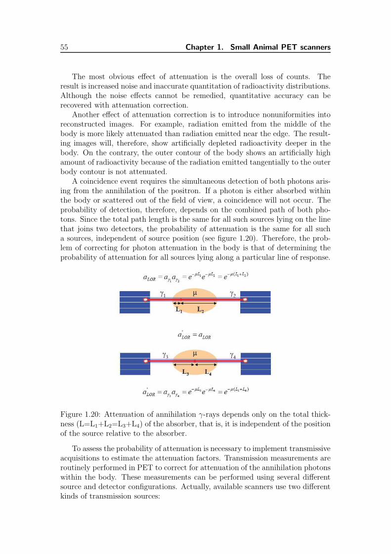
55 Chapter 1. Small Animal PET scanners
The most obvious effect of attenuation is the overall loss of counts. Theresult is increased noise and inaccurate quantitation of radioactivity distributions.Although the noise effects cannot be remedied, quantitative accuracy can berecovered with attenuation correction.
Another effect of attenuation correction is to introduce nonuniformities intoreconstructed images. For example, radiation emitted from the middle of thebody is more likely attenuated than radiation emitted near the edge. The result-ing images will, therefore, show artificially depleted radioactivity deeper in thebody. On the contrary, the outer contour of the body shows an artificially highamount of radioactivity because of the radiation emitted tangentially to the outerbody contour is not attenuated.
A coincidence event requires the simultaneous detection of both photons aris-ing from the annihilation of the positron. If a photon is either absorbed withinthe body or scattered out of the field of view, a coincidence will not occur. Theprobability of detection, therefore, depends on the combined path of both pho-tons. Since the total path length is the same for all such sources lying on the linethat joins two detectors, the probability of attenuation is the same for all sucha sources, independent of source position (see figure 1.20). Therefore, the prob-lem of correcting for photon attenuation in the body is that of determining theprobability of attenuation for all sources lying along a particular line of response.
Figure 1.20: Attenuation of annihilation γ-rays depends only on the total thick-ness (L=L1+L2=L3+L4) of the absorber, that is, it is independent of the positionof the source relative to the absorber.
To assess the probability of attenuation is necessary to implement transmissiveacquisitions to estimate the attenuation factors. Transmission measurements areroutinely performed in PET to correct for attenuation of the annihilation photonswithin the body. These measurements can be performed using several differentsource and detector configurations. Actually, available scanners use two differentkinds of transmission sources:

1.1. Basics of PET 56
1. 68Ge, which is a β+-emitter and the transmission data are collected ascoincidence events [68], [69].
2. 137Cs, in this case the source is a γ-emitter of 662 keV and the transmissiondata are collected using single events. When using this source, an additionalstep is necessary in order to account for energy difference (662 vs. 511keV) [70].
In the case of PET/CT scanners, the measurement of transmission data isperformed using the CT examination. The resulting data are taken at an energythat is very different from 511 keV, so the data must be scaled to use for theattenuation correction of the emission data.
Dead Time Correction
In general, PET scanners have a finite deadtime and associated count losses. Thedeadtime is the length of time required for a counting system to fully process andrecord an event, during which additional events cannot be recorded. As a result,the measured count rate is systematically lower than the actual count rate. Suchcount losses are significant, however, only at “high” count rates (i.e., greater thanthe inverse deadtime expressed in seconds). For multi-detector ring PET systems,deadtime count losses are generally minimal at clinical administered activities.Nonetheless, a real-time correction for deadtime count losses is routinely appliedto the measured count rates. Most commonly, this is performed by scaling upthe measurement count rate, either per LOR or globally, based on an empiricallyderived mathematical relationship between measured and true count rates.
Compensation for image degradation phenomena
Once the values for correcting the above mentioned degradation factors havebeen estimated using one of the methods described above, the estimated valuesare usually subtracted or multiplied to the prompts. In many clinical imple-mentations, the prompts are pre-corrected prior to the reconstruction step. Thepre-correction of the data is necessary when the analytical reconstruction meth-ods are used. Nevertheless, when working in the iterative framework, it is possibleand recommended to reconstruct directly the prompts data introducing the cor-rections within the reconstruction algorithm. In the iterative framework, thestatistical model of the emitted and detected data obeys the Poisson distribu-tion. When correction factors are applied to the raw data, this assumption is nolonger valid. For example, in the case of random coincidences correction, the sub-traction technique can be problematic and can reduce the accuracy of the imagereconstruction, as discussed in [112]. The reason of the reduction in accuracy isthat the iterative algorithms which have been developed using pre-corrected data(described by a shifted Poisson model [29]) are approximate in nature.
The expression of the MLEM algorithm with the relevant corrections included[112] is the following:

57 Chapter 1. Small Animal PET scanners
fm+1j =
fmj
∑Ii=1 ǫiaipij
I∑
i=1
ǫiaipij
di∑J
b=1 ǫiaipibfb + si + dr,i
, (1.33)
where
di(f) = dt,i + si + dr,i =J
∑
j=1
ǫiaipijfj + si + dr,i. (1.34)
Considering that the data are organized as a LOR histogram and the index icounts for the LORs, dt,i is the number of true coincidences at i, si refers to thenumber of scatter coincidences i, dr,i represents the random coincidences i, pij isthe element of the system matrix corresponding to LOR i and voxel j, and fj isthe value of the voxel j at the image. The normalization (ǫi) and the attenuation(ai) correction are multiplicative and they appear multiplying the elements ofthe system matrix pij . The variables I and J correspond to the total number ofLORs and the total number of voxels, respectively.
1.1.4 Image Quality
The ability to obtain images that help achieve a desired goal is the way to testan image reconstruction algorithm, a correction method or to validate the use ofan specific system matrix. Therefore, the image evaluation is called task-basedassessment. For example, if the task is quantitative, such a measurement oftracer concentration in a given image region, then the reconstruction algorithm,correction method or system matrix should be judged by its quantitative accuracy.Lesion detectability is another interesting task for our case and is one of the majorapplication of PET, then an algorithm, correction method or system matrix isconsidered to perform well if it produces images that lead to accurate diagnosis.Finally, if the task requires the ability to visualize small objects, the spatialresolution would be the corresponding metric.
The following figures-of-merit (FOM) were employed in this work to quantifythe quality of the reconstructed images, keeping in mind quantitative, lesiondetectability, and visibility of small details tasks:
1. Root Mean Square Error: A comparison between the emitted source andthe reconstructed image was performed using the root mean square error(ǫrms) defined as:
ǫrms =
[
1
M
M∑
m=0
(f (k)m − fm)2
]
1
2
(1.35)
where M is the total number of voxels, m is the voxel number, f (k)m and fm
are the counts in the reconstructed image at k iteration and the number ofphoton pairs emitted in the voxel m, respectively. Both are normalized tothe average voxel value.
2. Spatial Resolution: The full width at half maximum (FWHM) and fullwidth at tenth maximum (FWTM) of the radial and tangential profiles ofa point source were determined by linear interpolation.

1.1. Basics of PET 58
3. Discrepancy: The activity within a region of interest (ROI) was obtained bysumming the voxels in the ROI in the reconstructed images. The activityfound for this ROI in the reconstructed image (AROI), was compared withthe activity within the ROI in a reference image (Aref
ROI). The discrepancy(D) was calculated as
D(%) = 100AROI − Aref
ROI
ArefROI
, (1.36)
4. Mispositioned Events (ME): The number of events found within a ROI,where there should be no activity, were counted and divided by the totalreconstructed counts in the image
ME(%) = 100EventsNoAct−ROI
Eventsall
. (1.37)
The ideal ME value would be zero.
5. Signal-to-Noise Ratio (SNR): This is given by
SNR =|µROI1 − µROI2|
σROI2
, (1.38)
where µROI1 and µROI2 are the averages of the reconstructed voxels withintwo ROIs defined on the image, and σROI2 is the standard deviation of thevoxels of second ROI.
6. Background Noise (σbkg): This is the normalized standard deviation of thevoxel values within a background ROI (standard deviation divided by theaverage).
7. Contrast Recovery Coefficient (CRC): This is the value of the contrastbetween two ROIs normalized to the expected value for the contrast, Cideal:
CRC = 100
µROI1
µROI2
− 1aROI1
aROI2
− 1, (1.39)
where aROI1 and aROI2 are the activity concentration in the first and secondROIs respectively (see figure 1.21).
1.1.5 Monte Carlo Simulations
Monte Carlo (MC) methods are numerical calculation methods based on randomvariable sampling. The technique of random sampling to solve mathematicalproblems has been known since 1770. Only with the advent of quantum mechanicsin which matter-radiation interactions were interpreted using cross sections as

59 Chapter 1. Small Animal PET scanners
ROI1
ROI2
Figure 1.21: Example of ROI definition in a phantom that consists of a back-ground area and inside of it a hot region. The ROI1 and ROI2 are drawn in theareas under study of the phantom.
probabilities, the random sampling technique 2 was applied to nuclear physics.In the early 1960s, the Monte Carlo method was used by H.O. Anger to simulatethe physical response of his new scintillator camera. Since then, thanks to thepossibility of modelling different physical processes independently, the method hasbeen applied in medical radiation physics to a wide range of problems that couldnot be easily addressed using experimental or analytical approaches. NuclearMedicine Imaging, that deals with radioactive decay, the emission of radiationenergy through photons and particles, and the detection of these quanta andparticles in various materials, can benefit from the MC method. The simulationof the above mentioned processes based on the MC method are known as MonteCarlo simulations.
In Nuclear Medicine and particularly in Single Photon Emission ComputedTomography (SPECT) and PET, the use of Monte Carlo methods has the advan-tage of using general purpose codes developed for high energy physics or dosime-try. High-energy processes (>1 MeV), secondary and low-energy radiations couldbe neglected as they were not involved in SPECT and PET. On the other hand,the similarity of physical and geometrical characteristics of most emission tomo-graphs suggested specific models to be developed, thus favouring the creation ofcodes dedicated to simulations of emission tomography configurations.
Several SPECT/PET dedicated Monte Carlo software packages were devel-oped for simulating a variety of emission tomography studies. Among them,public domain codes have been made available in last years, allowing the use ofthe Monte Carlo method by the whole scientific community and even in the clin-ical environment. Several topics were addressed by Monte Carlo simulations inboth PET and SPECT, among which optimisation of imaging system design (in-cluding detector, collimator, and shield design), development of correction meth-ods for improved image quantitation, evaluation of correction techniques (scat-ter/randoms/attenuation correction, partial volume effect), development and as-sessment of image reconstruction algorithms, receiver operating characteristicstudies 3, pharmaco-kinetic modelling. Two types of Monte Carlo codes can be
2named “Monte Carlo method” because the Monte Carlo casino was the most famous centrefor playing games involving random drawing.
3This analysis is done to assess how well the medical images allow a human observer to

1.1. Basics of PET 60
Table 1.3: Main Monte Carlo codes currently available for SPECT and PETsimulations
Generic Codes
EGS4 (radiation dosimetry) [32]MCNP (radiation dosimetry) [33]
ITS (high energy physics) [34]GEANT 3 (high energy physics) [35]GEANT 4 (high energy physics) [36]
Dedicated codes
SPECT only: SIMIND [37]SimSPECT (derived from MCNP) [38] [39]
MCMATV [40] [41]PET only: PETSIM [42] [43]
EIDOLON [44]Reilhac [45]
PET-EGS [46]SPECT and PET: SIMSET [47] [48]
Dedicated based on Generic codes:
SPECT and PET: GATE (based on GEANT 4) [49] [50]
used for simulating SPECT and PET: 1)general purpose code, which simulate par-ticle transportation and were developed for high energy physics or for dosimetry,2)dedicated codes, designed specifically for SPECT or PET simulations. Table1.3 summarises the main codes currently available. General-purpose packagesinclude well-validated physics models, geometry modelling tools and efficient vi-sualization utilities. However, it is quite difficult to tailor these packages to PETand SPECT. On the other hand, the dedicated Monte Carlo codes developed forPET and SPECT suffer from a variety of drawbacks and limitations in terms ofvalidation, accuracy and support.
All Monte Carlo codes share some common components, such as random num-ber generator, rules to sample probability distributions, and sets of probabilitydensity functions. The features that make the codes different are related to theaccuracy, flexibility, efficiency and ease to use of the codes.
One of the limitations is that because the results are based on a computermodel, the accuracy of the results will depend on the accuracy of the model.The question one should always ask is whether the model includes all the factorsone would expect to affect the measurement in real situations (normalizationcorrection, decay time).
A major advantage of simulations in nuclear medicine imaging is that theyallow studies of parameters that are not measurable in practice (for example,
perform the specified task. The study plots the trade-off of false-positive and true-positive foran observer.

61 Chapter 1. Small Animal PET scanners
random coincidences in our case). In addition, in a computer model it is possi-ble to turn off certain effects, such as photon attenuation and scattering in thephantom.
Another fundamental requirement in MC simulations is access to randomnumbers. In theory, a random number cannot be predicted or calculated. Despitethis, the most common approach in computer simulations is to use a computerprogram to obtain randomly distributed numbers. These pseudo-random num-bers are calculated from previous numbers, which implies that there must be aoriginal number (seed) to initiate the random number sequence. Thus, startingtwo simulations with the same initial value will in the end produce the same result,even through random numbers are involved. Furthermore, because simulationsare performed on digital machines that use numbers limited to a known range(2, bytes, 4 bytes, 8 bytes, etc.), there is always a chance that a random numbersampled during the simulation will be equal to the initial value. The result willthen be a repetition of the random number sequence, which may have seriousconsequences for the accuracy of the results. Therefore, for Monte Carlo simu-lations, it is crucial that the generators have good randomness properties. Thisis particularly important for large-scale simulations done on high-performanceparallel computers.
GATE
GATE, the Geant4 Application for Tomographic Emission, is a Monte Carlosimulator that combines the advantages of the general-purpose Geant4 simulationcode [52] and of specific software tool implementations dedicated to emissiontomography. Indeed, GATE takes the advantage of the well-validated physicsmodels, of the geometry description, and of the visualisation and 3D renderingtools offered by Geant4. Furthermore, GATE integrates specific components tofacilitate its use in the PET/SPECT domain.
One distinctive and original feature of GATE is the modelling of time-dependentprocesses; synchronized with the evolution of the source activities and spatialdistributions [53]. Moreover, GATE includes a coherent management of parallelmultiple sources with independent time-profiles and locations.
The code comprises a large number of software components allowing it tomodel various aspects of nuclear medicine experiments: geometry, movement,detection, data output, etc. Users can choose among these components andassemble them interactively to set up simulations according to their own require-ments by using a scripting language. In addition, the users may specify anynumber of radioactive sources with different propierties (radioisotope, position,activity), which may overlap each other, as well as the detector geometry (forexample, natural radioactivity of the lutetium). GATE computes the full gammatracking from the vertex point to the end of the gamma range in the experimentalarea with Compton scattering, Rayleigh diffusion, and photoelectric effects. Anumber of modules are available for modelling the detection process, going fromthe detection of the gamma-rays by the scintillating crystals (singles) to the de-

1.1. Basics of PET 62
tection of coincidences in PET. Random events are tagged and may be processedindependently from the true coincidences. Scattering events in detector or inphantom can be tracked and stored in a list mode file output.
LHC Computing Grid Project
Although variance reduction techniques have been developed to reduce computa-tion time, the main drawback of the Monte Carlo method is that it is extremelytime-consuming. For example, one needs to track hundreds of millions of particlesto obtain the statistics required for image reconstruction studies. Consequently,a large amount of CPU time (weeks or even months) may be required to obtainuseful simulated data sets. As distributed or parallel computers are becomingincreasingly accessible to computational scientists, problems that may otherwisebe computationally prohibitive can be performed much faster than with a scalarmachine. Additionally, among all simulation techniques of physical processes, theMonte Carlo method is probably the most suitable one for parallel or distributedcomputing since photon histories are completely independent from each others.
The LHC Computing Grid Project (LCG) was born to prepare the comput-ing infrastructure for the simulation, processing and analysis of the data of theLarge Hadron Collider (LHC) experiments [54]. The LHC, which has been con-structed at the European Laboratory for Particle Physics (CERN), is the world’slargest and most powerful particle accelerator. The case of the LHC experimentsillustrates well the motivation behind Grid technology. The LHC acceleratorstarted operation in September 2008, and the experiments that will use it (AL-ICE, ATLAS, CMS and LHCb) will generate enormous amounts of data. Theprocessing of this data will require large computational and storage resources andthe associated human resources for operation and support. It was not consideredfeasible to fund all of the resources at one site, and so it was agreed that theLCG computing service would be implemented as a geographically distributedComputational Data Grid. This means that the service will use computing andstorage resources, installed at a large number of computing sites in many differ-ent countries, interconnected by fast networks. LCG-2 Grid middleware will hidemuch of the complexity of this environment from the user, giving the impressionthat all of these resources are available in a coherent virtual computer centre.The users of a Grid infrastructure are divided into Virtual Organisations (VO),abstract entities grouping users, institutions and resources in the same admin-istrative domain. The LCG-2 VOs correspond to real organisations or projects,such as the four LHC experiments; other VOs exist in the context of EGEE, likethe community of biomedical researchers, etc.
There is a Grid facility at the IFIC (Instituto de Fısica Corpuscular) conse-quence of a cooperation between the University of Valencia and CSIC (ConsejoSuperior de Investigaciones Cientficas). Two VOs are using this facility, the AT-LAS project and the IFIC. The IFIC VO is meant for researchers at IFIC thatwant to use the Grid resources. At the IFIC, there are 192 PCs connected with afast Ethernet. Each PC is a AMD Athlon of 1.2/1.4 GHz with 1 GByte SDRAM
63 Chapter 1. Small Animal PET scanners
and a harddrive UDMA100 of 40 GByte. Through a collaboration between theIFIC and the Klinikum rechts der Isar, we have been able to employ the compu-tational resources of this facility to run distributed Monte Carlo simulations.
1.2 Why small animal PET scanners?
Many of the traditional medical imaging technologies, including PET, are be-ing adapted for use in small laboratory animal imaging. PET can be viewed asan in vivo counterpart to autoradiography, tissue detection and other techniquesthat involve imaging or counting excised tissue samples taken from animals intowhich a radioactively labeled tracer has been introduced prior to sacrifice. Theadvantage of a non invasive imaging technique such as PET is that the entiretime course of the biodistribution or a radiolabeled tracer can be determined ina single living animal. Furthermore, that animal can be studied again at a latertime, permitting longitudinal, within-subject study designs to follow disease mod-els and interventions over periods of days, weeks, and even months. Because thesame animal is used at every time point, each animal serves as its own controland variability due to interanimal differences is effectively removed. Therefore,a single animal studied multiple times by PET may in some instances providethe same data that would have required tens of animals using traditional invasivetechniques that requires sacrifice of the animal. This clearly is in keeping withthe desire to reduce the number of laboratory animals used in experiments, butequally important, it has the potential to dramatically reduce the cost of experi-ments and to speed up the availability of results. It may also improve the qualityof the data (because of the within-subject design), although this has yet to beunequivocally demonstrated.
A large number of positron-labeled compounds have been synthetized [8] thusenabling a wide range of biological processes to be measured quantitatively, non-invasively and repeatedly using PET [9]. Combined with the very high sensitivityof radiotracer methods, this flexibility to interrogate living biological systems atthe level of specific enzymes, proteins, receptors, and genes makes PET extremelyattractive for studies in laboratory animals.
A final important advantage of using medical imaging techniques such asPET in small animal models of disease is that imaging provides a bridge betweenthe animal model and human studies. A valid concern in the use of animalmodels relates to how well that model predicts what will happen in the human.Techniques such as PET provide the opportunity to perform exactly the sameexperiments in mouse and human, facilitating direct comparison and appropriateinterpretation of the animal model data.
1.3 Challenges of small animal PET
Challenges common to all imaging techniques include (a) the design of probes orprobing techniques that are highly specific to the biological processes of interest,

1.3. Challenges of small animal PET 64
(b) optimization of imaging systems to provide the highest sensitivity and imageresolution, and (c) minimization of perturbation to the biological processes underobservation so that the experimental outcomes correlate to the biology and not theprobing process. There are a number of issues that must be carefully consideredin animal PET studies. Some of these have much in common with designingand optimizing PET scanners for human imaging; others are problems specificto small animal imaging. The underlying challenge, as always, is to obtain asmany counts as possible and to localize these counts as accurately as possible.Accurate localization of counts depends primarily on the spatial resolution ofthe detectors and the ability to remove or correct phenomena such as scatter,accidental coincidences, and pile-up that are incorrectly positioned. Maximizingthe number of detected counts requires injection of the maximum radioactivitypossible based on mass and specific activity considerations, and using an imagingsystem with high-efficiency detectors and large solid-angle coverage. The systemmust be able to run at high counting rates so that no counts are lost due todead time and it must also have a narrow timing window to minimize accidentalcoincidences. The first challenge to PET imaging technology clearly comes fromthe vast difference in physical size between the subject for which clinical PETsystems have been developed, the human (weight ∼70 kg), and the laboratoryrat (weight ∼300 g). This represents more than 200 fold decrease in volume.Laboratory mice, at 30 g, account for another order of magnitude decrease involume. Therefore to achieve similar image quality and to address the samebiological questions in mice that can currently be studied in humans, PET systemmust be developed with similar improvements in spatial resolution. This suggesta reconstructed spatial resolution <1 mm in all directions (<1 µl in volume)as opposed to the ∼10 mm (∼1 ml in volume) reconstructed image resolutiontypical in human whole body studies. This stringent requirement calls for newapproaches in both detector materials and design.
The absolute detection sensitivity of the imaging instrument (the fraction ofradioactive decays that result in a detected event) must be at least as good, andpreferably much better than, the typical PET scanner. Whole-body human PETscanners detect on the order of 0.3-0.6% of the coincident annihilation photonsin two-dimensional mode and 2-4% in 3D acquisition mode [10], [11]. For sensi-tivity it is clearly not possible to use the previous argument. Even with perfectlyefficient detectors and complete solid angle coverage around the animal, the bestwe can hope to achieve is about 200-fold increase in 2D mode and 30-fold in-crease in 3D mode. An approach to compensate for the sensitivity problem isto use more sophisticated reconstruction algorithms that make better use of theavailable counts. Iterative algorithms that accurately model the physics of thescanner and the statistics of the raw data will probably play an important rolein very-high-resolution PET studies because they can produce improvements ineither resolution or signal-to-noise relative to analytic reconstruction algorithms.Another approach can be to inject larger amounts of radioactivity, but there aresome fundamental issues that limit how far the dose can be raised and we willdiscuss them below. One might be tempted to think that because laboratory

65 Chapter 1. Small Animal PET scanners
animals are not subject to the same radiation exposure rules and procedures ap-plicable to humans, the injected activity per gram of tissue could be adjustedupward, thereby increasing the detected counts per resolution element and over-coming some of the sensitivity challenges outlined above. However, the wholeidea of a tracer kinetic experiment is that the mass levels are sufficiently low soas not to perturb the biological system under study. For a given specific activityof radiotracer 0, the injected mass is linearly proportional to the injected activity.There are many circumstances in which the tracer mass will limit the amountof radioactivity that can be injected into a mouse in the range of 0.037 to 3.7MBq [16]. The amount of mass that can be injected without violating tracerprinciples must be carefully determined on a case by case basis. There are casesin which relatively large amounts of radioactivity can be injected into an animal,in these cases dead time and count rate performance may become the limitingfactor. Other factors, such as energy resolution, dead time characteristics, theability to perform attenuation correction, and imaging field of view, pose differ-ent constraints to the design of detector and system and need to be taken intoconsideration.
The accuracy of the biological models derived from animal PET experimentsdepends on the quantitative accuracy of imaging. PET data needs to be cor-rected, notably for normalization, attenuation, scatter, and dead time, to achievequantitative images. The implementation of these correction techniques can beaffected by the choices of the system design. Compromises in performance charac-teristics are often necessary, and should consider the targeted applications of thesystem, the availability and cost of technologies, and the ease and cost operation.
1.4 Overview of this work
The following work has been dedicated to a specific small animall PET calledMADPET-II, developed at the Klinikum rechts der Isar in Munich. Unique fea-tures of MADPET-II are the crystals distribution in two radial layers and theindividual crystal read out by an avalanche photodiode. Chapter 2 discusses atlength the design and main features of this scanner. MADPET-II performanceallows us to obtain high sensitivity preserving high spatial resolution. High sen-sitivity is achieved by using a FOV as large as the inner diameter of the scanner,reducing the low energy threshold (LET) and introducing triple events. At thesame time, high spatial resolution is obtained providing DOI and reconstructingimages with LOR-based 3D iterative techniques (MLEM) with a Monte Carlosystem matrix. Two chapters of this thesis are reserved to study in more detailtwo of the above mentioned elements, the generation of the Monte Carlo systemmatrix (chapter 3) and the introduction of the triple events (chapter 5).
In general, small animal PET scanners are aimed at radiopharmaceutical stud-
0the fraction of the molecules in the tracer solution which are radiolabeled at a given timeand it is expressed in units Bq/g becquerels per gram or, more commonly, in concentrationunits of Bq/mol becquerels per mole

1.4. Overview of this work 66
ies. For these studies, it is very important that the reconstructed images providequantitative information about the activity within the subject under study. Sev-eral corrections must be taken into account in order to obtain realistic estimatesof the activity distribution. Among the latter, this thesis has focused in therandom coincidence correction (chapter 4) and normalization (chapter 6).
All the chapters of this thesis have a common denominator which is the useof simulations based on Monte Carlo techniques. We have taken advantage fromthe benefits of the Monte Carlo method and suffered its limitations. First of all,we are able to simulate a scanner which is very complex due to the dual layerconfiguration. Another advantage of the Monte Carlo technique is that it allowsstudies of effects that depend on parameters that are not measurable in practice.For example, we could test the validity of the random coincidences estimationmethods using the information related with the annihilation that is provided bythe simulation toolkit. In addition, in a computer model it is possible to switch onand off certain effects according to the focus of interest. For example, the scatterand attenuation inside the object was left aside when investigating the randomcoincidences to focus on the detector and system effects. For the normalizationstudy, we need a realistic simulation of the source and thus, we simulate the sourcewithin the container, including the attenuation and scatter within the object, andas well, the decay of the activity. An important limitation of the Monte Carlotechnique is the computing time required for the simulations. We have partiallysolved this problem by using the symmetries of the scanner and the distributedcomputers at the Grid facility in IFIC.
After the description chapter of the MADPET-II scanner, the outline of thiswork is as follows:
• Chapter 3 presents the creation of the Monte Carlo system matrix.
• Chapter 4 investigates the random coincidences correction.
• Chapter 5 includes the triple events for generating the images.
• Chapter 6 studies different approaches of normalization.
At the end of each chapter the conclusions are explained in English. The lastchapter summarizes the main conclusions in Spanish.
Chapter 2
MADPET-II
2.1 Objectives of the system
MADPET-II is a small animal scanner for radiopharmaceutical studies. Theconcept and design of MADPET-II improves both spatial resolution and sen-sitivity compared with conventional technology. These goals are achieved bymodifying traditional detector designs that may degrade the performance of theimaging device:
• Individual crystal readout in contrast to block detector. Block detectorsare replaced by individual crystal readout to avoid either event misposi-tioning (affecting spatial resolution) or count losses (reducing sensitivity)due to pile-up effects if multiple scintillation pulses are incident within ashort time [71]. The event mispositioning or count losses may result whenusing block detector, since every photodetector in a block reads the scin-tillation light from many crystals, more important at high incident gammaray flux. Additionally, with its individual crystal readout, the system candifferentiate those photons depositing some energy in a single crystal fromthose undergoing interactions in more than one unit (inter-crystal scatter,ICS). Block detectors assign to such ICS photon the LOR resulting fromthe weighted average over all the energy depositions within a block. Thismispositioning of the coincidence may lead to a resolution degradation. Onthe contrary, MADPET-II can distinguish and, if desired, disregard ICScoincidences. However, the contribution of ICS events to the sensitivitycan be significant and the degradation of spatial resolution due to the ICSevents can be solved by using an algorithm to identify the primary LOR.
• Crystals in dual-layer arrangement as compared to one layer. As it wasexplained in the introduction (see section 1.1.1) shorter crystals providebetter DOI information, thus better spatial resolution. On the contrary, thesensitivity is reduced for these crystals. To achieve high spatial resolutionit is necessary to use small crystals and to compensate for the decreaseof sensitivity a second layer of crystals is included. The two radial layersoffer the advantage of quantified, “binary” DOI information. Therefore,
67

2.2. System Description 68
the dual-layer configuration fulfil at once the requirements of high spatialresolution and high sensitivity.
• Singles list-mode acquisition unlike acquired data in sinogram format orcoincidence events in list-mode. The singles list-mode acquisition providesa tremendous amount of flexibility in generating images, because all the pa-rameters of interest can now be adjusted post-acquisition in software [73].Consequently, several images with different applied lower energy thresholdsor coincidence timing windows can be generated from a single data set ac-quired in a single scan. It is also possible to use intelligent algorithms in thecoincidence sorting stage that will decide to include or reject certain typesof coincidence events based on user-defined criteria such as high resolutionor high sensitivity.
2.2 System Description
Front-end architecture
Figure 2.1: Crystal distribution of the MADPET-II scanner as reproduced byMonte Carlo simulations (left) and the arrangement of the 18 dual layer detectormodules in the complete system (right).
MADPET-II consists of 18 dual layer detector modules arranged in a ring (seefigure 2.1). The axial and radial extent of the tomograph is 18.1 and 71 mm re-spectively, allowing for mouse and rat imaging. Each detector module consists oftwo layers: Front and back. For each dual layer detector module, the front layercontains a 4×8 array of 2×2×6 mm LSO crystals, each optically isolated (usinga 3M Radiant foil) and coupled one-to-one to a monolithic 4×8 avalanche photo-diode (APD) array (Hamamatsu), shown in figure 2.2. The back layer is read outindependently, and is similar to the front layer, apart from the radial size of theLSO crystals, which is 8 mm in this case. The APD pixel sensitive area is 1.6×1.6mm2 and the interspacing between units is 0.3 mm. The coupling between each
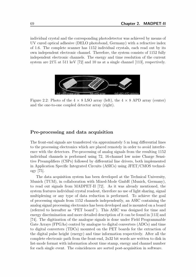
69 Chapter 2. MADPET-II
individual crystal and the corresponding photodetector was achieved by means ofUV cured optical adhesive (DELO photobond, Germany) with a refractive indexof 1.6. The complete scanner has 1152 individual crystals, each read out by itsown independent electronic channel. Therefore, the system consists of 1152 fullyindependent electronic channels. The energy and time resolution of the currentsystem are 21% at 511 keV [72] and 10 ns at a single channel [113], respectively.
Figure 2.2: Photo of the 4 × 8 LSO array (left), the 4 × 8 APD array (center)and the one-to-one coupled detector array (right).
Pre-processing and data acquisition
The front-end signals are transferred via approximately 5 m long differential linesto the processing electronics which are placed remotely in order to avoid interfer-ence with the detectors. Pre-processing of analog signals from the resulting 1152individual channels is performed using 72, 16-channel low noise Charge Sensi-tive Preamplifiers (CSPs) followed by differential line drivers, both implementedin Application Specific Integrated Circuits (ASICs) using JFET/CMOS technol-ogy [75].
The data acquisition system has been developed at the Technical University,Munich (TUM), in collaboration with Mixed-Mode GmbH (Munich, Germany),to read out signals from MADPET-II [72]. As it was already mentioned, thesystem features individual crystal readout, therefore no use of light sharing, signalmultiplexing or any type of data reduction is performed. To achieve the goalof processing signals from 1152 channels independently, an ASIC containing theanalog signal processing electronics has been developed and is mounted on a board(referred to hereafter as “PET board”). This ASIC was designed for time andenergy discrimination and more detailed description of it can be found in [113] and[74]. The digitization of the analogue signals is done under Field ProgrammableGate Arrays (FPGAs) control by analogue to digital converters (ADCs) and timeto digital converters (TDCs) mounted on the PET boards for the extraction ofthe digital pulse height (energy) and time information respectively. After all thecomplete electronic path from the front-end, 2x32 bit words are written to disk inlist-mode format with information about time stamp, energy and channel numberfor each single event. The coincidences are sorted post-acquisition in software.

2.2. System Description 70
Identification of Coincidences
Emulating the measurements performed with MADPET-II, each simulation pro-duces an output file listing the detected singles and coincidences are sorted afteracquisition according to the detection time [73]. Unlike the measurements, moreinformation about the single event than time, energy and channel number isavailable in the simulation files. The sorting starts with the first single of thelist which opens the first time coincidence window (prompt window), where τ isthe window width. Then, the number of singles within τ is determined. Thisprocedure is repeated until the end of the singles list.
Figure 2.3: Two examples of possible coincidences in MADPET-II. The coin-cidence characterized by the LOR1 is a valid coincidence because satisfies thegeometrical condition. Whereas, the LOR2-coincidence, defined by two crystalsfrom adjacent modules, do not satisfy the geometrical condition. Thus, this co-incidence would be excluded.
Coincidences are organized according to the following criteria:
1. The number of singles m in τ are counted, excluding the one that opens thewindow. The case m = 1 is considered a double coincidence (double) whilem = 2 is a triple coincidence (triple). In this work, values of m higher than2 were not classified (multiple coincidences).
2. To exclude coincidences arising from the same annihilation photon throughICS, a geometrical condition is applied (see figure 2.3). Most of the singles

71 Chapter 2. MADPET-II
produced by the same photon are usually detected within the same dual-layer module or in adjacent ones. Coincidences that involve singles detectedin the same (or adjacent) dual-layer module are labeled as not physicallymeaningful (NP) and are not taken into account for image reconstructionpurposes. Coincidences that involve different, non-contiguous modules areconsidered as valid coincidences because the LOR described by the singleevents is physically meaningful. If two singles are detected in two non-contiguous dual-layer modules and within the time coincidence window,this double coincidence is considered a prompt. In the case of m = 2, atriple, the geometrical condition must be satisfied by at least two singles.
3. Using the information provided by GATE (EventID), a random or truecoincidence can be identified. If all singles within τ , including the onethat opens the time coincidence window, have the same EventID, all comefrom the same annihilation process, and this coincidence is labeled as a true(double or triple true coincidences depending on m). A random coincidenceis identified when at least one single has a different EventID than the others(double or triple random coincidences depending on m).
The complete procedure for coincidence sorting is outlined in figure 2.4.
Figure 2.4: Outline of the coincidence sorting process. The horizontal axis repre-sents the time evolution, and each vertical line marks the time of a single event.
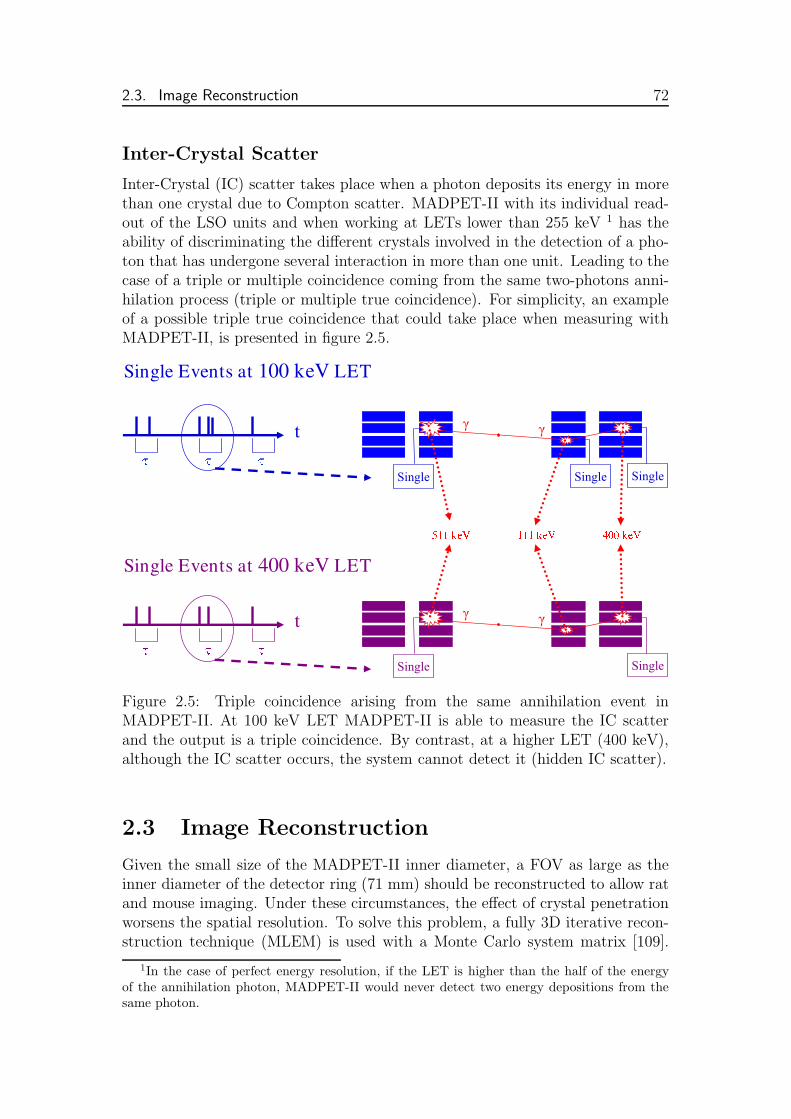
2.3. Image Reconstruction 72
Inter-Crystal Scatter
Inter-Crystal (IC) scatter takes place when a photon deposits its energy in morethan one crystal due to Compton scatter. MADPET-II with its individual read-out of the LSO units and when working at LETs lower than 255 keV 1 has theability of discriminating the different crystals involved in the detection of a pho-ton that has undergone several interaction in more than one unit. Leading to thecase of a triple or multiple coincidence coming from the same two-photons anni-hilation process (triple or multiple true coincidence). For simplicity, an exampleof a possible triple true coincidence that could take place when measuring withMADPET-II, is presented in figure 2.5.
Figure 2.5: Triple coincidence arising from the same annihilation event inMADPET-II. At 100 keV LET MADPET-II is able to measure the IC scatterand the output is a triple coincidence. By contrast, at a higher LET (400 keV),although the IC scatter occurs, the system cannot detect it (hidden IC scatter).
2.3 Image Reconstruction
Given the small size of the MADPET-II inner diameter, a FOV as large as theinner diameter of the detector ring (71 mm) should be reconstructed to allow ratand mouse imaging. Under these circumstances, the effect of crystal penetrationworsens the spatial resolution. To solve this problem, a fully 3D iterative recon-struction technique (MLEM) is used with a Monte Carlo system matrix [109].
1In the case of perfect energy resolution, if the LET is higher than the half of the energyof the annihilation photon, MADPET-II would never detect two energy depositions from thesame photon.

73 Chapter 2. MADPET-II
The coincidence data were organized in LOR histogram, to keep the spatial in-formation. Additionally, all the studied corrections in this thesis were appliedwithin the reconstruction algorithm (see section 1.1.3).
2.3.1 Simulations with GATE
In this work we have used extensively Monte Carlo techniques by means of GATEfor studying various aspects related to the image reconstruction process. Forthese simulations, the geometry and main characteristics of MADPET-II havebeen emulated. In order to speed up the simulations, two photons of 511 keVemitted in opposite directions were generated for each annihilation event, insteadof creating the positron and posterior the annihilation. A time resolution of 10 nsand energy resolution of 21% at 511 keV were included to reproduce the responseof the scanner. The low energy threshold was set to 100 keV, while the upperenergy threshold was at 700 keV.


Chapter 3
System Matrix for MADPET-II
As it was already explained in the introduction (section 1.1.2), iterative recon-struction algorithms require the computation of the system matrix (SM) P, whichrepresents the imaging process. This chapter is dedicated to show how the SMcan be built by means of Monte Carlo techniques, and the high quality imagesthat provide the combination of a Monte Carlo SM with an iterative reconstruc-tion algorithm MLEM. The comparison of two different system matrices for adifferent energy window in terms of image quality is also presented in order todecide which energy window produces the best results.
3.1 Monte Carlo System Matrix
In PET, the elements of the system matrix, pij, represent the probability ofdetecting an annihilation event emitted from the image voxel j by the LOR idefined by a detector pair. The probability depends on the range of the positron,the non-collinearity of the annihilation photons, the scatter and attenuation ofthe photons within the object to image, the scatter of the photons in the detectorring, the efficiency of the scintillator crystals, etc. If one wants to include allinvolved effects, even for the case of 3D small animal PET, the system matrixbecomes huge. Sparseness and symmetries can be use to reduce the size to morereasonable proportions. Additionally, factoring the system matrix in componentsthat account for the different physical effects is another way to handle the sizeproblem [76], [77]. The decomposition could be done as follows:
P = Pdet.effPdet.scatterPattPgeomPpositron (3.1)
From the last expression, one can see that there are factors that depend onthe scanner (Pdet.eff , Pdet.scatter, and Pgeom), on the object (Patt) and on theradio-isotop being used (Ppositron).
As first approximation, the elements of the system matrix could be assessedby computing the intersection of the LOR with each voxel; this simplified modelallows that the weights of the SM can be calculated on-the-fly [78]. More precisemethods consider the position of the voxel relative to the detectors [79], or useanalytical models or empirical kernels to correct for parallax error [80], [81], [82].
75

3.2. Generation of the System Matrices 76
The correct way of calculating the SM would be to make a set of measurementsof a point source within the scanner. However, this would take a huge amount oftime to acquire good statistics and the need of having the system running beforetesting the reconstruction algorithm. Nevertheless, a simplified approach of thecorrect way was performed by [83] (an the extension to fully 3D PET in [84]),making a reduced number of point source measurements and extracting in a veryelaborate manner the overall SM. Our approach for high resolution 3D PET inorder to increase the reconstruction quality is to use Monte Carlo techniques [85][86], in this way the forward process of the measurement is precisely modelled.
Monte Carlo simulations allow to obtain a realistic complete response ofMADPET-II, before the system was built, providing a way to check some featuresand to optimize the image reconstruction algorithm and corrections. Thereforethis is the chosen approach for MADPET-II. However, there are some limitationsin our choice. One of these limitations is that the matrix elements are affected bystatistical noise, due to the random processes involved in a MC simulation. Theeffect of the noise propagation into the image from the elements of the SM couldbe reduced by increasing the number of simulated events [110]. Another limita-tion is related to the storage of the SM elements, due to the number of LORs andimage voxels, the size of the SM will be very large. To overcome this drawback,optimization of the format in which the SM is stored in relation to the calculationsused in the reconstruction algorithm is necessary. Finally, a general limitation ofthe MC simulations, because of the results are based on a computer model, theaccuracy of the results will depend on the accuracy of the model. GATE is thesimulation code employed in this work and there are several publications thatvalidate the model in which is based [87], [88], [89], [90], [91], [92], [93].
3.2 Generation of the System Matrices
As we have mentioned, the SM has been built using MC simulations (MCSM)by means of the software named GATE. The FOV has a cylindrical shape whoseradius is 35 mm (RFOV = 98%Rscanner) and is 20 mm long. The FOV is dis-cretized in 140×140×40 cubic voxels of 0.5×0.5×0.5 mm3 volume and centeredat the middle of the scanner (figure 3.1). An individual simulation for each voxelthat belongs to the cylindrical FOV is performed to generate the SM. In total,from the 784000 voxels that form the cubic array, a number of 615200 voxels fitinto this FOV. For the simulations, the voxels are considered cubic sources of 0.5-mm side. Within each voxel, 2 million positron annihilations were created. Thisnumber was chosen for two reasons. The first one was to increase the statisticsof a previous MCSM [109]. The second was to obtain the MCSM in a reasonabletime. To speed up the computations, the annihilations were emulated sendingtwo photons back-to-back, without considering the emission of the positron, thepositron range, and the non-collinearity.
After the simulation of an individual voxel the output contains the single

77 Chapter 3. System Matrix for MADPET-II
70 mm
Figure 3.1: Representation of the FOV inside of a 3D array of voxels. The voxels,whose center is inside of the red circle, are for image reconstruction.
events detected at 100 keV LET 1. First of all, a LET higher than 100 keV isapplied to the singles list. Coincidences were sorted according to the detectiontime t and the criteria explained in chapter 2. If the number of the singles withinτ (m) is 1 and this single belongs to the same annihilation (same EventID) asthe single that opens the time window, a LOR is assigned to this coincidence ifthe geometrical condition is satisfied. Then, we obtain the number of detectedcoincidences in that LOR i for each voxel j, cij. The cij are called non-normalizedcoefficients or weights of the SM. The probabilities of the SM (pij) are calculateddividing cij between the 2 million simulated annihilations:
pij = cij/2 · 106. (3.2)
In our approach, the non-zero elements cij are stored and the correspondingpij are calculated in the reconstruction algorithm. In this way, the storage of theSM is reduced by using integers for the non-normalized coefficients (cij).
We focus on two different situations to build the SM:
• Considering double true coincidences (double trues) for a LET of 200 keV(SM-200).
• Working double trues and 400 keV LET (SM-400).
These two LETs are interesting for the MADPET-II scanner because they rep-resent two different frameworks. At 200 keV LET, inter-crystal scatter (photonsthat undergo Compton scatter and deposit its energy in more than one crystal)is present and can be measured by MADPET-II (due to its individual crystalreadout). On the contrary, increasing the LET to 400 kev makes that the inter-crystal scatter is not detected. Additionally, at lower LET the sensitivity of thescanner is higher. But, the spatial resolution could be affected by the increase of
1In a real acquisition, to maximize the flexibility of MADPET-II, a very low energy thresholdis set in hardware. Our intention in the simulations was to mimic the measurements and,therefore, they are done with the same LET.

3.2. Generation of the System Matrices 78
scattered events in the scanner 2. Therefore, our goal is to determine under whichcircumstances (inter-crystal scatter and higher sensitivity versus no scatter andlower sensitivity) the reconstructed images with higher quality are obtained.
By using MC simulation to generate the SM, the elements of the created SMinclude the factors that account for the geometry of the scanner and the scatterin the detector (Pdet.scatter and Pgeom). The factor Pdet.eff is studied in chapter 6and it needs from measurements to obtain the coefficients. In the case of smallanimal PET, as MADPET-II, the noncolinearity of the two photons coming fromthe annihilation is negligible (resolution loss is 0.0022×70 ≈ 0.015 mm). Relatedto the range of the positron, if we consider 18F studies, the positron range for thisradio-isotope is in the sub-millimetre. Therefore, the Ppositron can be set equalto the identity matrix. In any case, if necessary, the range of the positron canbe included in the model a posteriori. Finally, Patt is object-dependent and theattenuation factors can be calculated or measured for each object being scanned.
3.2.1 Matrix Symmetries
It is possible to increase the statistical quality of P by applying the symmetriesinherent in the combination of MADPET-II system and the voxelized FOV (seefigure 3.2). Considering the transaxial plane and a centered grid, the value relatedto the weight pij corresponding to voxel j (purple square at the top right) andLOR i (top right solid line) is the same as for pkl, where k and l are the valuesof the LOR and the voxel after the reflections about the Y axis. These elementscan also be reflected about the X axis to obtain pmn and pop. Additionally, fourmore identical values can be found after reflection about the OXY plane. Thevoxels corresponding to 1/8 of the whole FOV were simulated (see figure 3.7)and by exploiting the mentioned symmetries, all the elements of the SM can beobtained. In this way, the necessary time to reproduce the SM and the space tostore it is reduced by 8 times.
3.2.2 Use of Grid
After using the symmetries, the number of voxels to be simulated is 76900. Thus,realistic simulations to build the SM would take approximately 534 days (con-sidering that the simulation of a voxel would need, in average, 10 minutes) in asingle CPU computer. However, these simulations are excellent candidates forthe parallel solution to the computational problem, because there is no need ofinter-process communication. Providing that we have access to the Grid resourcesat the IFIC (143 PCs), the simulations to generate the SM have been performedfully in these computers. The time necessary for these simulations was 90 days.As we can see, the theoretical, linear speed-up is not achieved due to many fac-tors. The most important factor is that these PCs are shared between the usersof two VOs, ATLAS and IFIC. The users of the ATLAS VO have a 70% priority
2Also in the object, but this has not been studied in this thesis

79 Chapter 3. System Matrix for MADPET-II
Figure 3.2: Symmetries in MADPET-II system for a cartesian voxelized FOV.
in use, whereas the users at the IFIC VO only 30%. Other factors are the timespent in the submission of the job and getting the output data, and there is alimit in the number of jobs that a user can send. Nevertheless, we speed up ina factor of almost 6, that makes a “reasonable” time to obtain the data for theSM.
3.2.3 Storage of the System Matrix
As we have already mentioned, the size of system matrix in the case of 3D ac-quisition is very large. Taking into account that the SM is a sparse matrix, it ispossible to save some space by storing only the non-zero elements. Nevertheless,the precalculated non-zero elements of the SM need to be stored in large filesthat cannot be loaded into the RAM and, therefore the reconstruction algorithmneeds a lot of time to read the elements of the SM from file for each iteration.Through a collaboration with computer scientists at the TU-Munich, a formatwas developed to optimize the storage of the SM in order to make faster thereconstruction algorithm. This format had a header, where relevant informationabout the SM is provided, like the maximal LOR number or the emitted annihi-lations (all the information contained in the header is shown in figure 3.3). AnLOR array follows the header, where an offset for a given LOR is stored. Thisoffset indicates the address, where the information related to this LOR (the cor-responding voxels and weights) is found. When the LOR has no entries the offsetis the same that the previous one. After the LOR array comes an structure thatis repeated as many LOR with entries. The structure contains the maximum

3.3. Characterization of the System Matrices 80
non-normalized weight for this LOR (cmaxij ), then cmax
ij + 1 offsets into the voxeldata and the voxel data for this LOR. The first offset corresponds to the addresswhere the voxels that have cij = 1 can be found. The second indicates where thevoxels, that have a non-normalized weight of 2 counts, start and so on. Finally,the voxel data for this LOR follows the voxel offsets. With this new format thedisk space is notably reduced and the reconstruction time is feasible.
Figure 3.3: Schema of the optimized format employed to store the system matrix.The color lines are drawn to show where the offsets (memory addresses) arepointing. After the header, there is an array of LOR offsets. This array hasLORmax+1 elements, each pointing to the memory position where the informationrelated to the corresponding LOR is stored. As an example, in the figure is shownthe first black arrow that is starting at Offset0 and ending at the position in whichthe maximum number of counts for the 0-LOR is found. The same is indicatedwith the blue arrow for the Offset1 for the 1-LOR. The structure and informationthat is stored for each LOR is the following: first the maximum number of countsfor this LOR (cmax
LOR), then another array of cmaxLOR offsets, and finally the voxel
data. The second black arrow in the figure is indicating where the voxels thathave one count for the 0-LOR are saved. The red arrow points to the voxels withmaximum counts for the 0-LOR.
3.3 Characterization of the System Matrices
We have employed the following parameters to characterize the two system ma-trices, prior to evaluation of the quality of the reconstructed images that the SMsprovide,

81 Chapter 3. System Matrix for MADPET-II
• The number of non-zero matrix elements, Nnon−zero.
• The mean relative error, defined as
σrel =
∑I−1;J−1i=0;j=0
σcij
cij
Nnon−zero
, (3.3)
where σcijis the standard deviation of the detected counts (cij) by the LOR
i emitted from voxel j. Assuming that the detection of the photons is aPoisson process, it is possible to write σcij
=√
cij .
• The sensitivity is defined as the ratio between the true coincidences detectedby the scanner for a voxel at the center of the FOV (jc) and the emittedannihilations (Nea)
S = 100˙∑I−1
i=0 cijc
Nea
. (3.4)
• Disk space occupied by the SM in the optimized format.
3.4 Effect of the Low Energy Threshold on Im-
age Reconstruction
3.4.1 Simulated Sources
To study the image quality obtained by using the two system matrices (SM-200and SM-400), the following sources have been simulated:
• A Derenzo-like phantom was used for visual analysis of the image quality.This phantom consists of 6 sectors containing 20 mm long rod sources withdiameters of 1, 1.3, 1.5, 1.8, 2.4 and 3.2 mm and rod separation twicethe diameter. The rod sources were spread within a cylinder of 62 mmdiameter (see figure 3.4). The activity concentration of this source was2.52 MBq/cm3. The acquisition time of the simulation was 900 s (thedetected events were 1.15×10⁸ and 4.38×10⁷, for 200 keV and 400 keVLET, respectively).
• Point sources covering half of the radial FOV were simulated to estimate pa-rameters related to the spatial resolution. The point sources were sphericaldistributions of 0.125 mm radius. The sources were separated by a distanceof 5 mm. The activity of each source was 1.85 MBq and the simulation wasacquired during 120 s.
• Hot-cold-background (HCB) phantom was employed to analyse quantita-tively the quality of the images reconstructed using both SMs. This phan-tom is a 3.7-MBq cylindrical source of 20 mm long and 30 mm radius(background region). There are two rods inside the cylinder. One of the

3.4. Effect of the Low Energy Threshold on Image Reconstruction 82
rods does not contain activity (cold rod) and the other has 1.54 MBq (hotrod). The centers of the rods are situated at (0,-15,0) and (0,15,0) mm, forthe cold and hot regions respectively. Both rods are cylinders of 10 mmradius and 19.5 mm. The activity concentration ratio between the hot rodand the background was 1:3 and the acquisition time is 600 s. Inside thehot-cold-background source three regions of interest (ROI) were defined, ahot, cold and background ROI corresponding to the hot rod, cold rod andbackground regions respectively (figure 3.5). The three ROIs are 8 mm longcylinders with diameters of 16 mm. These ROIs were used to quantify thequality of the reconstructed images based on the figures-of-merit describedin section 1.1.4.
Figure 3.4: Derenzo-like phantom simulated using GATE to investigate the qual-ity of the reconstructed images. The phantom is organized in 6 sectors. Eachsector is made up of 20 cm long rod sources with diameters of 1, 1.3, 1.5, 1.8, 2.4,and 3.2 mm and rod separation twice the diameter.
Figure 3.5: Hot, cold, and background ROIs in the hot-cold-background source.All ROIs are 8 mm long cylinders with diameters of 16 mm. Diameter of thesource cylinder is 60 mm, and diameter of rods is 20 mm.
In order to focus on the image quality that the SMs can provide, there wasno attenuation media in the simulated sources, therefore we do not reproducethe scatter, nor attenuation within the object. Another reason that supports thisapproximation is that the contribution of the object scatter for a small animalPET scanner is small in comparison to the detector scatter ( [94], [95], [96], [97]).

83 Chapter 3. System Matrix for MADPET-II
3.4.2 Image reconstruction
As we have mentioned, we use MLEM reconstruction algorithm to reconstruct theimages combined with the Monte Carlo SM. The code employed for this purposewas optimized in order to run in a reasonable time using the large file, wherethe SM was stored. All the sources described in this section were reconstructedusing this algorithm. Additionally, as we were interested in quantifying the spa-tial resolution, the point sources were reconstructed using the 3D ReprojectionAlgorithm (FBP3D) that implements Kinahan and Rogers FBP algorithm withreprojection of the missing data [27], provided by the open source Software forTomographic Image Reconstruction (STIR, [100]).
3.4.3 Figures-of-Merit
The system matrix is the basis of the iterative algorithm. Therefore, to estimatewhich is the SM that provides better images for MADPET-II, we need to useFOMs according to the tasks that MADPET-II was designed for:
1. Quantitation: For the evaluation of the images according to this task, thediscrepancy, the mean square error, and the misspositioned events, definedat the introduction (section 1.1.4, 57), were employed for the hot-cold-background phantom, using the known emitted source as a reference.
2. Lesion Detectability: Computing the CRC vs. the background noise or theSNR for the hot-cold-background phantom (the hot region would simulatethe lesion among the background activity) can reflect the performance thatmay be achieved for this task (defined in section 1.1.4, 57).
3. Small details visibility was assessed by means of the FWHM and the FWTM(used to express the spatial resolution as presented in section 1.1.4, 57) forthe reconstructed images of point sources using MLEM and FBP3D.
3.5 Results: Comparison of the System Matri-
ces
3.5.1 Characteristics of the System Matrices
From the 153.8×10⁹ total emitted annihilations to generate the SM, 1.49×10⁹
detected coincidences were found in the SM at 200 keV LET and 5.44×10⁸ forthe 400 keV LET case. Taking into account the voxels that are inside the FOV,from where the annihilations were emitted, the mean valued of detected eventsper voxel is 19510.8 and 7128.4 for 200 keV and 400 keV LET, respectively. Theaverage of the detected events per LOR, considering only the LORs that at leasthave one detected event, is 3206.56 for the 200 keV LET case and 2128.41 for400 keV LET case. The number of LORs with at least one detected event was464886 and 255885, for 200 keV and 400 keV LET, respectively.

3.5. Results: Comparison of the System Matrices 84
For the SM at 200 keV LET, the maximum number of detected events perLOR and per voxel was 97 and the average of detected events over the nonzeroelements was 2.72. This can be understood due to the fact that over 71% ofthe non-zero matrix elements were related to only one detected pair of photonsper LOR and per voxel, i.e. cij = 1. This situation is not so extreme in thecase of 400 keV LET, where the maximum was found to be 59, the average was3.26 counts per voxel and LOR and the percentage of elements with one countwas 43%. This situation can be very well seen in the figure 3.6. In these plotsthe contribution from a voxel to an specific LOR is represented (cij), then theleft-right and up-down symmetries were applied to obtain the complete LOR. Inthe plots corresponding to the 200 keV LET case, voxels spread from all over theFOV contribute to the LOR, whereas in the situation of 400 keV LET, the voxelsare concentrated in the area defined by the LOR.
200 keV 400 keV
Figure 3.6: Plots corresponding to the contribution of each voxel that belongsto a certain slice to a specific LOR represented in the label of the plot. Thecomplete LOR has been drawn by using the symmetries, because only the voxelsthat belong to 1/8 of the FOV were simulated.
The situation seen in the plots at 200 keV LET is a consequence of the LETused. Setting the low energy threshold at 200 keV allows that photons that havescattered previously in other detector crystal could produce a detected event onlydepositing a part of its initial energy. This produces a contribution from a voxelout of the LOR volume to this LOR. As it can be seen from the values, thesecontributions had very low probability, the values of these elements usually were1 or 2 detected annihilations per voxel and LOR.
Finally, to end up with the characterization of the two SMs, the main prop-erties of the SMs are shown in table 3.1. In this table, it can be seen that thestatistical quality of the SMs at 400 keV LET is higher than at 200 keV, althoughthe number of detected events is less. This is due to the elements with one countin the SM at 200 keV. Indeed, for 200 keV LET, if the elements with one count are
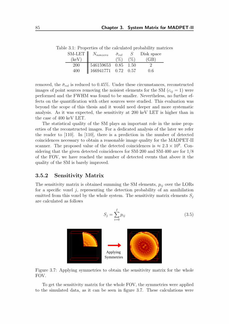
85 Chapter 3. System Matrix for MADPET-II
Table 3.1: Properties of the calculated probability matrices
SM-LET Nnonzero σrel S Disk space(keV) (%) (%) (GB)200 546159653 0.85 1.50 2400 166941771 0.72 0.57 0.6
removed, the σrel is reduced to 0.45%. Under these circumstances, reconstructedimages of point sources removing the noisiest elements for the SM (cij = 1) wereperformed and the FWHM was found to be smaller. Nevertheless, no further ef-fects on the quantification with other sources were studied. This evaluation wasbeyond the scope of this thesis and it would need deeper and more systematicanalysis. As it was expected, the sensitivity at 200 keV LET is higher than inthe case of 400 keV LET.
The statistical quality of the SM plays an important role in the noise prop-erties of the reconstructed images. For a dedicated analysis of the later we referthe reader to [110]. In [110], there is a prediction in the number of detectedcoincidences necessary to obtain a reasonable image quality for the MADPET-IIscanner. The proposed value of the detected coincidences is ≈ 2.3 × 10⁹. Con-sidering that the given detected coincidences for SM-200 and SM-400 are for 1/8of the FOV, we have reached the number of detected events that above it thequality of the SM is barely improved.
3.5.2 Sensitivity Matrix
The sensitivity matrix is obtained summing the SM elements, pij over the LORsfor a specific voxel j, representing the detection probability of an annihilationemitted from this voxel by the whole system. The sensitivity matrix elements Sj
are calculated as follows
Sj =I
∑
i=0
pij (3.5)
SymmetriesApplying
Figure 3.7: Applying symmetries to obtain the sensitivity matrix for the wholeFOV.
To get the sensitivity matrix for the whole FOV, the symmetries were appliedto the simulated data, as it can be seen in figure 3.7. These calculations were

3.5. Results: Comparison of the System Matrices 86
performed for both cases, 200 and 400 keV LET. The sensitivity matrix for thevoxels that belong to the central slice are represented in figure 3.8 for the studiedcases. The two pictures on the left are normalized to the same maximum, theone corresponding to the 200 keV case. From these images is obvious that thescanner at 400 keV LET is less sensitive, as we expected. As a consequenceof lower sensitivity at 400 keV LET, the sensitivity matrix shows higher noisefor this LET, as it can be seen in the most right plot. On the other hand,the sensitivity matrix of both cases has the same flower-like structure and twointernal rings, this is more visible on the two extreme plots. This structure isdue to the association of the crystals in 18 modules and the empty spaces (nodetector crystals) between them. Indeed the petals of the flower shape are 18, likethe number of modules. And the rings are coincident with the missing samplingdue to the distance between detector modules, shown in figure 3.10 at the left bythe area under the blue lines. Another common characteristic is that the valueof the sensitivity matrix is increasing radially from the center to the edges ofthe FOV. The reasons of this behaviour are that the voxels towards the FOVedge have larger solid angle (see figure 3.9) and more effective crystal thickness.The increase of the effective crystal thickness can be understood qualitatively,thinking in an ideal detector ring (figure 3.10 at the right) and considering thatthe probability of detection is proportional to the distance travelled by the photonwithin the detector ring. The annihilation photons leaving a voxel at the centerof the ring pass through the ring, all covering the same distance, the width of thering. Whereas, the annihilation photons emitted from a voxel at the edges of theFOV travel across the ring a larger distance than the width of the ring. Whichmeans, the photons from the edge of the FOV have a higher probability to bedetected.
3.5.3 Spatial Resolution
The point sources covering half of the radial FOV and the Derenzo-like phantomwere used to study and compare the spatial resolution attained with the two SMs.The reconstructed images of both phantoms are shown in figures 3.11, 3.12, and3.13. As we can see from the figure of the Derenzo-like phantom, there is nosubstantial differences between the reconstructed images using the SMs at 200keV LET and at 400 keV LET, not only in the reconstructed images, but alsoin the profiles through the sectors of 2.4- and 1.5-mm diameter rods (at the left)and 3.2 and 1.3 rods diameter (at the right). For both SMs, the smallest rodstructure of the Derenzo-like phantom that can be identified is the correspondingto the 1.5 mm rods diameter. It is possible to distinguish the 8 rods of the 1.5mm diameter rods sector from its profile for the two studied cases of SM.
To quantify the spatial resolution across the radial FOV, the projections ofthe point sources were reconstructed using FBP. As first step the sources werereconstructed using FBP without any rotation during the acquisition, because thescanner is not meant to rotate. The results of this first step can be seen in the firstrow of figure 3.13. Due to the gaps between the detectors there are null elements

87 Chapter 3. System Matrix for MADPET-II
(a) LET = 200 keV (b) LET = 400 keV
Figure 3.8: Top: Sensitivity Matrix of the central slice for the two studied cases.Bottom: Profiles of the sensitivity matrices (left) and the ratio of both profiles(right).
in the sinogram and these missing data are creating the “star” artifacts thatwe can see in these images. The artifacts prevent from calculating the FWHM(neither the FWTM) from these images to quantify the spatial resolution. Thesecond step, done in order to solve this problem, was to rotate the scanner duringthe simulation (it can be done also by rotating the source). This was proposedin [98] and [99] to recover the missing data. By doing this, the reconstructedimages shown in the second row of figure 3.13 were obtained. Although, thereare still some artifacts due to the non-uniformity in the sensitivity of the LORsand to remove them it is necessary to normalize. However, it is still possible toasses the spatial resolution for these images.
As we have mentioned that we plan to reconstruct the images using MLEMand the Monte Carlo SM, the corresponding reconstructed images using MLEMand the two SMs are also presented in figure 3.13 and the FWHM and FWTMwere also calculated from the profile of these images to compare with the resultsobtained using FBP. The point sources in the MLEM reconstructed images areperfectly visible and there are no artifacts close to them. Only the two pointsources closest to the edge of the FOV are blurred. For these images there is

3.5. Results: Comparison of the System Matrices 88
������������
α
β
α < β
Figure 3.9: The solid angle seen by the voxels increases as the voxels are closerto the edge of the FOV. In this figure it is shown the solid angle for a centralvoxel (α) and for a excentrical voxel (β). The solid angle for the voxel closer tothe edge of the FOV is larger than the one for the central voxel.
Figure 3.10: Graphical explanation of the flower-like shape of the sensitivitymatrix (left) and the increase of Sj towards the edge of the FOV (right). In theimage at the right, it is observed that the central black ring is coincident to theundersampled areas due to the space between detectors (dark-blue lines). On theleft, it is shown the intersection of the photon pair path with an ideal detectorring. The cyan lines correspond to cases that the incidence is not perpendicular,whereas the dark blue lines are for the orthogonal incidences. Considering thatthe probability of detection is proportional to the travelled distance of the photonin the detector, the voxels closer to the edge have higher probability.
a slight difference between the reconstructed images using the SM at 200 keVLET and 400 keV LET, the point sources are blurrier for the case of 200 keVLET, more obvious at the edges of the FOV. The reason of this behaviour can

89 Chapter 3. System Matrix for MADPET-II
(a) Transverse (b) Coronal (c) Sagittal
(d) P1 (e) P2
Figure 3.11: Reconstructed images (top) and profiles (bottom) of the Derenzophantom, using 100 iterations of MLEM at 200 keV LET.
be predicted from the figure 3.6: Due to the lower LET, there are contributionsfrom voxels outside the tube defined by the two detectors and these elements ofthe SM make that the point sources at 200 keV LET are slightly more spread.This is an example of limitation in the ability of the SM to compensate for thedegradation effects. Although the detector scatter is modelled on both SMs, theresults achieved for the 400-SM are better than for 200-SM, because the detectorscatter is more notable at 200 keV LET.
The profiles of the second and third row of the figure 3.13 were used to cal-culate the FWHM and the FWTM, and the calculated values versus the radialposition are represented in figure 3.14. In general the values of the FWHM andFWTM are always slightly better for the reconstructed images at 400 keV LET.The reason is what we have pointed out in the previous paragraph, related to theincrease of detector scatter when working at 200 keV LET. Comparing FBP andMLEM reconstructed images is obviously better the combination of MLEM withthe Monte Carlo SM, this was already seen in the figure 3.13. Nevertheless, thereare two points corresponding to the FBP reconstructed images that show lowerFWHM compare to the MLEM reconstructed images, as we can see in the plotof the figure 3.14. The reasons of this unexpected behaviour are different for thedifferent point sources. When reconstructing using the FBP algorithm provided

3.5. Results: Comparison of the System Matrices 90
(a) Transverse (b) Coronal (c) Sagittal
(d) P1 (e) P2
Figure 3.12: Reconstructed images (top) and profiles (bottom) of the Derenzophantom, using 100 iterations of MLEM at 400 keV LET.
by STIR, the zero position should be at the center of the bin. In this way thepoint source at the center is fully contained in the central voxel. Whereas in theMLEM reconstructed images, the central point source is shared between the twomost central pixels. This is the reason of the smaller value of the FWHM for theFBP in the central point source. The second unexpected values corresponds tothe 6th point source and the reason in this case is the artifact observed in theimage. This artifact is producing a second lower peak in the profile of this pointsource and this creates that the linear interpolation is done before this secondlower peak, making narrower the FWHM. In the FWTM plot, it is more visiblethe difference between the reconstructed images at 200 keV and 400 keV LET.
3.5.4 Quantification
The Hot-cold-background phantom was used to determine the quantification andlesion detectability capabilities of these two SMs. The reconstructed images andthe corresponding activity distribution are shown in the figure 3.15. At first sight,the main difference between the reconstructed images of both LETs is the highernoise of the image at 400 keV LET, due to the lower sensitivity at this LET. Thiscan be seen, not only in all the views of the reconstructed image (transversal,

91 Chapter 3. System Matrix for MADPET-II
Figure 3.13: Reconstructed images and profiles of the point sources using FBPwithout rotation, FBP with scanner rotation (20 steps of 1o) and 100 iterationsof MLEM for 200 (left) and 400 (right) keV LET.
0 5 10 15 20 25 300.51.01.52.02.53.03.5
50% FOV
FWH
M (m
m)
Radial Position (mm)
200 keV LET, MLEM (100th Iter.)
400 keV LET, MLEM (100th Iter.)
200 keV LET, FBP
400 keV LET, FBP
85% FOV
0 5 10 15 20 25 300.51.01.52.02.53.03.5
200 keV LET, MLEM (100th Iter.) 400 keV LET, MLEM (100th Iter.)
50% FOV
FWTM
(mm
)
Radial Position (mm)
200 keV LET, FBP 400 keV LET, FBP
85% FOV
Figure 3.14: FWHM (left) and FWTM (right) as a function of the radial positionfrom the profiles of the reconstructed images using FBP with scanner rotation(20 steps of 1o) and 100 iterations of MLEM for 200 and 400 keV LETs.
coronal and sagittal), but also in the profile shown at the last column of thefigure 3.15.

3.5. Results: Comparison of the System Matrices 92
Figure 3.15: Emitted source (top) and reconstructed images of the hot-cold-background phantom (view: transversal, coronal and sagittal), using 100 itera-tions of MLEM for 200 (center) and 400 (bottom) keV LET.
According to the analyzed FOMs (except for the ME) the 200 keV SM pro-vides a superior image quality than the 400 keV LET SM. The reason of thisbehaviour is the higher noise of the SM at 400 keV LET. The noise is higherbecause the 400-SM and the LOR histogram for this LET have less counts thanthe 200 keV LET. In order to compensate for the lower number of counts, weshould increase the number of simulations for the SM to get the same counts perLOR than at 200 keV and the time of the acquisition of the hot-cold-backgroundsource.
At figure 3.16 the ǫrms is represented for the different iterations. The recon-structed images are compared to the emitted source to obtain ǫrms. It is observedthat this error is higher for the case of 400 keV LET, as we expected. Comparingthe absolute reconstructed activity to the absolute emitted activity in the hot andbackground ROIs (figure 3.17) using the discrepancy (D(%)), it is observed thatwe can recover the emitted activity using both SMs (the maximum discrepancyvalue is 1%), but the SM at 200 keV LET provided closer values to the reference.Looking at the plots of the figure 3.19, it is also seen that the reconstructed im-ages at 400 keV LET show worse results due to the higher noise: The SNR islower in the plot at the left and the background noise (σBKG) is bigger at the rightplot on the figure 3.19. The CRC has been also plotted for different iterations,

93 Chapter 3. System Matrix for MADPET-II
but it is not shown here, because the same information can be seen in the rightplot of the figure 3.19. For both cases, the CRC reaches its maximum at the 30thiteration (the first point of the right plot at the figure 3.19 corresponds to the10th iteration) and there are no big changes from this iteration. Related to theME, despite that the difference is small, the reconstructed images at 200 keVLET show higher values, which means higher number of mispositioned events.The reason of these barely higher values is the contribution of voxels outside thetube of response, like in the spatial resolution section.
0 20 40 60 80 100
1500
2000
2500
3000
3500
rms
Iteration
200 keV LET 400 keV LET
Figure 3.16: Root mean square error of the reconstructed images using MLEMfor 200 (red) and 400 (blue) keV LET compared to the emitted source.
0 20 40 60 80 100-3.5-3.0-2.5-2.0-1.5-1.0-0.50.0
DH
OT(%
)
Iteration
200 keV LET 400 keV LET
0 20 40 60 80 100-3.5-3.0-2.5-2.0-1.5-1.0-0.50.0
DB
KG(%
)
Iteration
200 keV LET 400 keV LET
Figure 3.17: Discrepancy of the activity of the reconstructed images calculatedusing true coincidences and the emitted source within the hot (left) and back-ground (right) ROI for 200 and 400 keV LETs as a function of the number ofiterations.

3.6. Conclusions 94
0 20 40 60 80 1000.00
0.25
0.50
0.75
1.00
ME(
%)
Iteration
200 keV LET 400 keV LET
Figure 3.18: Mispositioned Events within the cold ROI for 200 and 400 keV LETsas a function of the number of iterations.
0 20 40 60 80 10068
1012141618
SNR
Iteration
200 keV LET 400 keV LET
0.10 0.15 0.20 0.25 0.30
98
99
100
101
102
CR
C(%
)
BKG
200 keV LET400 keV LET
Figure 3.19: SNR for 200 and 400 keV LETs as a function of number of iterations(left) and CRC versus σBKG for both LETs (right).
3.6 Conclusions
In this chapter we have shown how the system matrix for MADPET-II usingMonte Carlo techniques by means of GATE can be generated. One of the ob-stacles that this task poses is the computing time. In order to reduce this time,the symmetries of the system and distributed computing have been employed.One of the characteristic of MADPET-II is the flexibility of the acquired datagranted by the singles list mode. This facilitates the sorting of coincidences bysoftware using different parameters. Among the parameters that we can varypost-acquisition in MADPET-II, we have focused on the low energy threshold.The main reason is because the LET plays a very important role in the sensi-tivity of the scanner. By lowering the LET, we have a gain in the sensitivitybut, at the same time, there is an increase of detected scattered photons in the
95 Chapter 3. System Matrix for MADPET-II
detector and in the object 3. The increase of scatter can deteriorate the spatialresolution. The main aim of this chapter was to analyze the images at differentLETs, chosen as 200 and 400 keV. For each LET the detectors of the scannerresponds differently, thus requiring specific system matrices, denoted by SM-200and SM-400 throughout this chapter.
Some words about the obtained sensitivity matrices are appropriate beforediscussing the results of the reconstructed images. We have used the same simu-lation time to build the two SMs and, as a consequence of the higher sensitivityat 200 keV LET, the sensitivity matrix at this LET is less noisy than at 400 keVLET. For a fair comparison between both SMs, we would need to increase thetime of the simulations for the SM-400 to achieve the same noise level. It is nev-ertheless interesting to contrast the performance of the SM-200 and the SM-400when the same time has been invested in creating both.
Let us now turn to the analysis of the reconstructed images. In terms of spatialresolution, there are almost no observable differences in the Derenzo reconstructedimages, and the smallest rods that can be distinguished in both cases are theones of 1.5 mm diameter. When assessing the FWHM of the reconstructed pointsources, some differences appear for the point sources at the edges of the FOV.The SM-400 provides better spatial resolution (smaller values of the FWHM)for the point sources close to the edge of the FOV. From this result, we canconclude that the detector scatter present in the SM-200 has a higher impact onthe reconstructed image resolution than on the overall image noise. The statisticalnoise is higher for 400-SM, but the noise introduced by the detector scatter dueto mispositioning of the events is notably less and this produces a better FWHM,FWTM and ME.
When analyzing the FOMs for quantitation and lesion detectability, the SM-200 gives better performance. Clearly, the higher statistical noise in the SMand also in the input LOR histogram at 400 keV LET are the factors whichproduce this outcome. The conclusion of this part is that higher sensitivity, whichmeans lower statistical noise for the same acquisition time, is very important forquantitation of the activity distribution and lesion detectability.
The statistical noise in the input LOR histogram can be reduced by increasingthe acquisition time in the measurement at 400 keV LET. This was not studied,but it is important to keep in mind that there are examinations which are boundedto short time frames, like in the dynamic studies for pharmacokinetic modelling.In addition, it is very important to know the concentration of the tracer for thesestudies and a lower LET provides more accurate information for the activitydistribution. On the other hand, for static studies, where we are not limited toshort time frames, working at 400 keV LET would provide better images in termsof visibility of the small details. For the quantitative analysis at 400 keV LET,simulations with longer running time for the system matrix are required to reachthe performance of the SM-200.
3As we have already mentioned in the section 3.4.1, the scatter of the photons inside theobject for a small animal PET scanner has a less important effect for the reconstructed imagesthan the scatter in the detector, and has not been considered in this work.

3.6. Conclusions 96
From the results shown in this chapter, we can conclude that the flexibilityprovided by the singles list-mode output of MADPET-II is a very useful feature,because one can adapt the low energy threshold to the type of study in order toobtain the best results for the specific task.

Chapter 4
Random Coincidences Correction
An accidental or random coincidence (random) takes place when two photonscoming from different annihilations are detected within the same time coinci-dence window and mistakenly assigned as coincidence event (prompt). Randomcoincidences can contribute substantially to the background in PET. Accurate es-timates of radioactivity distributions within a patient or rodent from PET imagescannot be provided unless the effect of these coincidences is taken into account ina quantitative manner [3]. Several methods are commonly used for randoms cor-rection. They have been explained in the introduction, section 1.1.3. The goal ofthis chapter is to investigate the validity of the techniques for random coincidenceestimation for various low energy thresholds (LETs). For this investigation, sim-ulated list-mode data for MADPET-II are used as input. The simulations havebeen performed using the GATE simulation toolkit. Since the GATE simulationsallow random and true coincidences to be distinguished, a comparison betweenthe number of random coincidences estimated using the standard methods, andthe number obtained using GATE is performed. The random coincidence cor-rection can be applied in two different ways. One can subtract the estimatedrandoms from the prompts before the reconstruction. Or the randoms correctionis applied in the reconstruction algorithm. We compare the two approaches inthis chapter. The last part of the chapter is dedicated to the effect of the activityon the randoms estimation methods and correction. Most of the results shown inthis chapter are published in [101].
4.1 Randoms Estimation Methods for MADPET-
II
There are several methods to estimate random coincidences. The most com-mon technique is to acquire single events arriving within a delayed-coincidencewindow defined such that the probability of a true coincidence is zero [3]. Themethod is based on the assumption of constant time distribution of random co-incidences. This technique provides an accurate but noisy estimation for randomcoincidences [103]. A second method, called “singles-based” [103] estimation of
97

4.1. Randoms Estimation Methods for MADPET-II 98
random coincidences, calculates the mean random coincidence rate Rij for eachline of response (LOR) (or sinogram element related to detectors i and j) by usinga relationship between the singles rate in these detectors and the time coincidencewindow width, as explained in section 1.1.3. A third method uses the timing his-togram of the prompt coincidences [106], which shows an almost flat tail and thistail can be fitted to a linear function. As it was shown in section 1.1.3, the totalnumber of random coincidences can be obtained integrating the fitted functionwithin the corresponding time interval. In what follows, these three random es-timation methods for different low energy thresholds applied to the small animalPET scanner MADPET-II were investigated. In the case of the DW method, twodifferent modalities were used and they are explained in the following section.
4.1.1 Approaches to the Delayed Window method
Two approaches have been implemented for this method. In the first approach(which we call DW), the singles list-mode data were processed using two timewindows of the same size separated by a time interval (∆T ). The first windowwas the time coincidence window and the second was the delayed window. Forrandoms estimation, the number of singles m found in the delayed window wascounted and classified according to the conditions (i) and (ii) described in section2.2. Condition (ii) was applied to the single that opened the prompt window andthe single or singles found within the delayed window.
In the second approach (DW’), the singles data were duplicated by delayingthe time information of each single by a fixed amount ∆T , as presented in [114].Then, the delayed singles were added to the original data stream. The delayedsingles carry a flag that distinguishes between original (not delayed) and du-plicated (delayed). The combined data stream was sorted with only one timewindow (time coincidence window). Only non-delayed singles can open the timecoincidence window. Within this window, the singles n carrying a delayed flagwere counted. After the geometric condition is applied to the LOR described bythe single that opens the window and the delayed singles, n = 1 refers to the caseof double randoms while n = 2 corresponds to triple randoms. In this work, thecases n > 2 has not been considered.
Schemes representing the two approaches are presented in figure 4.1.
4.1.2 Simulations to study the performance
In this study, several sources were used to compute the total number of randoms(figure 4.2 and table 4.1). The sources represent various geometries, namely apoint-like source (Small Sphere), a planar source (Plane), a linear source (NEMARat-like), and a cylindrical source (Hot-Cold-Background). The small sphere andplane source were chosen to see the influence of the source geometry in the ran-dom estimation methods. The Rat-like source was based on the National Electri-cal Manufacturers Association (NEMA) NU2-2001 Performance Measurements ofPositron Emission Tomographs, with the source dimensions scaled down to the

99 Chapter 4. Random Coincidences Correction
Figure 4.1: Two different approaches of the randoms estimation methods basedon the delayed window concept. The first approach uses only the original singleschain. The second approach employs the original and the delayed singles chain(top). The horizontal line in both approaches shows the time evolution of themeasurement (bottom). The time coincidence window is denoted with τ . Thedelay applied to the delayed window is expressed with ∆T . The solid verticallines (|) represent the singles of the original chain. The arrows (↑) are the singlesof the delayed chain.
size of a standard rat. The NEMA rat-like source is a line source situated at17.5 mm offset from the central axis with radius and length 1.05 and 140 mmrespectively.
(a) (b) (c) (d)
Figure 4.2: Various source geometries simulated with GATE to study randomsestimation methods (see table 4.1 for dimensions).
The hot-cold-background source (figure 4.2b) was simulated, not only to anal-yse the performance of random coincidences estimation methods, but also to studythe effects of the methods on the reconstructed image. This source was a 20 mmlong, centred cylinder of 60 mm diameter without attenuation media and filled

4.1. Randoms Estimation Methods for MADPET-II 100
Table 4.1: Simulated sources.
Source Position Dimensions(mm) A(MBq) T (s)a Small Sphere centered r = 1 3.7 60b Hot-Cold-Back. centered r = 30, h = 20 3.7 + 1.59 600c Plane centered x = 2, y = 40.3, 3.7 60
z = 26.5d Rat-like 17.5 mm offset r = 1.05, h = 140 3.7 60
with activity (background, 3.7 MBq). Inside this cylinder two rods were placed,a cold rod without activity, and a hot rod with 3 times the activity concentrationof the background (1.59 MBq). Both rods had the same dimensions (19.5 mmlength and 20 mm diameter). The hot rod was located in the lower half of thecylinder while the cold rod was in the upper half (see figure 4.2b). For imagereconstruction purposes, the acquisition time for this source was 600 s. Inside thissource three ROIs were defined like in the previous chapter (figure 3.5). The threeROIs were cylinders, whose dimensions were 8-mm height and 16-mm diameter.These ROIs were used to quantify the quality of the reconstructed images basedon the figures-of-merit described in section 1.1.4.
To investigate the influence of the activity in the random estimation methods,simulations for various activity concentrations within the hot rod and backgroundkeeping constant the 3:1 ratio were carried out. The total activity of the back-ground cylinder ranged from 3.7 MBq to 111 MBq.
The expression for MLEM in equation 1.31 (page 48) with the MCSM pre-sented in chapter 3 was used for obtaining the reconstructed images from thesesimulations. For this study, in order to focus on random correction, the simulatedobject has no attenuation media. Therefore, there is nor scatter, neither attenu-ation in the object and it is not necessary to take them into account, si = 0 andai = 1. Several reconstructions of the same set of data (double coincidences) wereperformed for the different values of the random coincidences obtained using theDW and SR methods, for two LETs (200 keV and 400 keV) and for 100 iterations.Additionally, the case of using pre-corrected data (DW or SR) for reconstructionhas been studied. These images are referred to as DWSub or SRSub respectively.
4.1.3 Figures-of-Merit
To quantify the quality of the reconstructed images, the following figures-of-meritwere employed (all of them defined in section 1.1.4):
1. Discrepancy (D), calculated using the hot and background ROIs defined infigure 3.5; the reference is the reconstructed image obtained employing onlythe true coincidences. The reconstructed images with and without randomscorrection are compared to reference.
2. Mispositioned Events(ME)

101 Chapter 4. Random Coincidences Correction
3. Signal-to-Noise Ratio (SNR)
4. Background Noise (σbkg)
5. Contrast Recovery Coefficient (CRC)
4.2 Results
In this paragraph we describe the outline of the results part of this chapter.When studying the DW and SR randoms estimation methods for MADPET-IIdata at lower LET, it was observed an overestimation in the number of randomcoincidences. The randoms overestimation is presented in the section 4.2.1 fordifferent sources simulated with GATE. We have seen that this overestimationdecreases for LETs higher than 255 keV and it is reduced when the single eventswhich have undergone a Compton interaction in crystals before being detected areremoved from the data. These two facts lead us to infer that the overestimationis due to the inter-crystal scatter (explained in section 4.2.2). Including triplecoincidences could be a possible solution to solve this problem and some data thatsupport this option are shown in section 4.2.3. The effect of this overestimationon the reconstructed image is studied for a hot-cold-background source with 3.7MBq totat activity in the background region and 1.59 MBq total activity in thehot region in section 4.2.4. Finally the last section (4.2.5) is dedicated to analyzethe effect on the overestimation when changing the source activity.
4.2.1 Overestimation of the Random Coincidences
In figure 4.3, the total number of double randoms (dr) obtained from thesimulations of the planar source using GATE information, dgate
r , is comparedwith the double randoms estimated using the DW, DW’, SR, and TH methods(ddw
r , ddw′
r , dsrr , dth
r , respectively), by calculating the ratio dmethodr /dgate
r . Ideally,this ratio should be 1. The graphs show that the number of randoms for the DW,DW’, and SR methods is higher than dgate
r . It can be seen that the overestimationof randoms is higher for lower LETs. In the case of LETs higher than 250 keV,the agreement between ddw
r , ddw′
r , and dsrr with dgate
r is better and is not changinglargely when varying the LETs. For the case of TH, the estimated randoms areslightly lower than dgate
r , unlike the other methods. The observed overestimationfor DW and SR does not change substantially for the different τ values, except thecurves of the SR method at the two lowest LETs (100 and 150 keV). Therefore τwas set to 20 ns in the analysis that follows, which is twice1 the time resolution at asingle channel of the system to ensure that almost all the double true coincidencesare within this window.
As an aside, it is interesting to calculate the ratio between the total numberof double randoms in the simulation, dgate
r , and the prompts, dp, for the different
1The width of the time coincidence window is traditionally chosen to be twice the system’smeasured time resolution

4.2. Results 102
DW DW’ SR TH
Figure 4.3: Ratio between dr estimated with DW, DW’, SR, and TH methodsand dr obtained using GATE information as a function τ for a planar source andfor different LETs.
sources. This ratio is presented in figure 4.4. It is observed in these plots thatthe percentage of randoms is increasing for higher LETs for the same source.Comparing the sources, the point source is the one that has the lowest value ofthis ratio. This can be explained as follows. In general, we could differentiatetwo types of random coincidences. One type would be the random coincidencescreated because one of the photons is not detected although it has passed throughthe detector crystals. The other type would correspond to the case in which thephoton is not detected because there is not detector in its path2. Considering thepoint source at the center of the FOV, only the first type of random coincidencesis geometrically possible and they are less probable. The source with higherpercentage of randoms is the NEMA rat-like, due to the fact that almost all theactivity of the source is outside the FOV. Comparing the plane source with theHot-cold-background source, the latter has higher ratio of randoms because it has
2In both types, it is necessary that a second annihilation is produced and one of the photonsgoes undetected.
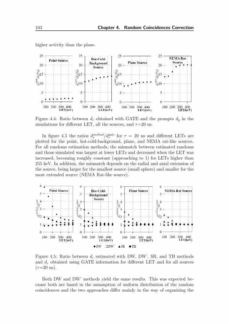
103 Chapter 4. Random Coincidences Correction
higher activity than the plane.
Figure 4.4: Ratio between dr obtained with GATE and the prompts dp in thesimulations for different LET, all the sources, and τ=20 ns.
In figure 4.5 the ratios dmethodr /dgate
r for τ = 20 ns and different LETs areplotted for the point, hot-cold-background, plane, and NEMA rat-like sources.For all randoms estimation methods, the mismatch between estimated randomsand those simulated was largest at lower LETs and decreased when the LET wasincreased, becoming roughly constant (approaching to 1) for LETs higher than255 keV. In addition, the mismatch depends on the radial and axial extension ofthe source, being larger for the smallest source (small sphere) and smaller for themost extended source (NEMA Rat-like source).
Figure 4.5: Ratio between dr estimated with DW, DW’, SR, and TH methodsand dr obtained using GATE information for different LET and for all sources(τ=20 ns).
Both DW and DW’ methods yield the same results. This was expected be-cause both are based in the assumption of uniform distribution of the randomcoincidences and the two approaches differ mainly in the way of organizing the

4.2. Results 104
data. In the DW, only the original singles chain is used with two time windows(coincidence and delayed time window). Whereas in the DW’, the sum of theoriginal plus the delayed singles chain is employed with only one time window.The effect of varying the delay in the DW’ method is shown in figure 4.6. Fordifferent values of ∆T (150, 200, 300 and 500 ns), the number of double ran-doms was compared with the number of double randoms for the reference delay,which is ∆T = 100 ns. As illustrated in figure 4.6, the randoms estimation isalmost independent of the delay. The discrepancy between the values obtainedfor different delays and the reference is smaller than 2% for all LETs.
Figure 4.6: Ratio between randoms estimated using the DW’ method with somedelay, ∆T , and the reference delay (∆T = 100 ns).
4.2.2 Effect of the Inter-Crystal Scatter
Photons that have undergone a Compton interaction in different crystals (ICscatter) are present in the data for LETs lower than 255 keV [108]. For example,for 200 keV LET, the number of scattered singles in the front layer is 9-10%(external rings) to 20-21% (central rings) higher than the number of singles thathave been detected without a previous Compton interaction in a crystal, for allthe studied sources. These IC scatter singles coming from one annihilation photonincrease the singles rate in a crystal producing a direct effect on the SR method,because singles that not only produce double coincidences but also triple andmultiple coincidences were used in this method. In order to apply the method,one needs to use all the singles in each channel. These triple coincidences couldbe both trues and randoms for a LETs lower than me/2 ≃255 keV. But the tripletrue coincidences rarely3 occur at a LET higher than 255 keV and hence the triplecoincidences can only be randoms. In addition, if IC scatter singles are present,the probability of finding a single in the delayed window increases. In relationto the TH method, it is necessary to open a wider time window (100 ns) and
3Triple true coincidences at higher LET than 255 keV could be possible due to the energyresolution. In an ideal detector, these coincidences would not take place above 255 keV LET.

105 Chapter 4. Random Coincidences Correction
to find only prompts (two singles in two non-contiguous modules) to make thetime histogram. In the presence of IC scatter singles, there are more triples andmultiples (more than 3 singles in the time window), consequently the numberof double randoms estimated with the TH method is less than the number ofrandoms obtained with GATE. The latter facts suggest that the IC scatter couldhave an impact on the random estimation methods. To test this possibility, theeffect of removing the IC scatter singles from the singles data was analyzed andthe modified data were processed again. To identify the IC scatter singles, theGATE variable ComptonCrystal defined in section 2.2 was used. The singlesfrom the initial data that had ComptonCrystal equal to zero were the ones beinganalyzed in this section. By doing this, the results shown in figures 4.7, 4.8,and 4.9 were obtained. The mismatch for the DW and DW’ methods almostdisappears (figure 4.7), and that for the SR method is substantially reduced(figure 4.8). Thus, the effect of IC scatter is notable when using DW and SRmethods at lower LETs. These results also show that the IC scatter impact isconsiderably reduced at high LETs (above 255 keV, where there is no possibilitythan a photon produces more than one single). The results also improve in thecase of the TH method (figure 4.9), although the mismatch obtained with ICscatter was not as high as for the other methods.
Figure 4.7: Ratio between dr estimated with DW and DW’ methods and withGATE (τ =20 ns, ∆T =100 ns), for several LETs and with and without ICscatter events.
4.2.3 Including triple random coincidences
A possible approach for random estimation applied to MADPET-II for lowLETs would be to estimate the percentage of IC scatter singles present in themeasurement and remove it, previous to coincidence sorting. However, this strat-egy implies a substantial decrease in sensitivity. Another approach, which willbe examined in more detail in chapter 5, would be to include the triple prompts(defined in section 2.2) in the coincidence sorting. The results shown in figure

4.2. Results 106
Figure 4.8: Ratio between dr estimated with SR method and with GATE, forseveral LETs and with and without IC scatter events (τ =20 ns).
Figure 4.9: Ratio between dr estimated with TH method and with GATE for τof 20 ns, for several LETs and with and without IC scatter events.
4.10 motivate this approach. In this figure the total number of triple (two singlesfound in the delayed window, tDW
r ) and double randoms estimated with DW,and the total number of triple (tgate
r ) and double randoms obtained using GATEinformation is compared. The mismatch is dramatically reduced for LETs higherthan 200 keV as compared with the data with IC scatter of figure 4.7. Thus,the estimation of random coincidences (combining double and triple randoms)using the DW method is closer to the values obtained with GATE informationfor the combined double and triple random coincidences. The posterior randomcorrection involving these triple prompts should be addressed elsewhere. In thecase of the SR method, in order to take into account the triple randoms, either anew expression for the random coincidences rate should be derived or the singlesshould be sorted differently. Both options are beyond the scope of this work andwill not be further discussed. In the rest of the chapter, we focus only in doubles(prompts, trues, and randoms) and the triple coincidences are studied in more
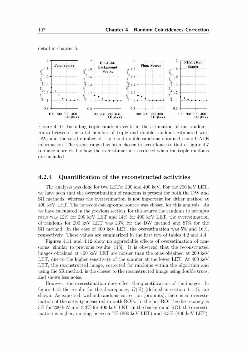
107 Chapter 4. Random Coincidences Correction
detail in chapter 5.
Figure 4.10: Including triple random events in the estimation of the randoms.Ratio between the total number of triple and double randoms estimated withDW, and the total number of triple and double randoms obtained using GATEinformation. The y-axis range has been chosen in accordance to that of figure 4.7to make more visible how the overestimation is reduced when the triple randomsare included.
4.2.4 Quantification of the reconstructed activities
The analysis was done for two LETs: 200 and 400 keV. For the 200 keV LET,we have seen that the overestimation of randoms is present for both the DW andSR methods, whereas the overestimation is not important for either method at400 keV LET. The hot-cold-background source was chosen for this analysis. Aswe have calculated in the previous section, for this source the randoms to promptsratio was 12% for 200 keV LET and 14% for 400 keV LET, the overestimationof randoms for 200 keV LET was 23% for the DW method and 87% for theSR method. In the case of 400 keV LET, the overestimation was 5% and 16%,respectively. These values are summarized in the first row of tables 4.2 and 4.4.
Figures 4.11 and 4.12 show no appreciable effects of overestimation of ran-doms, similar to previous results [115]. It is observed that the reconstructedimages obtained at 400 keV LET are noisier than the ones obtained at 200 keVLET, due to the higher sensitivity of the scanner at the lower LET. At 400 keVLET, the reconstructed image, corrected for randoms within the algorithm andusing the SR method, is the closest to the reconstructed image using double trues,and shows less noise.
However, the overestimation does effect the quantification of the images. Infigure 4.13 the results for the discrepancy, D(%) (defined in section 1.1.4), areshown. As expected, without randoms correction (prompts), there is an overesti-mation of the activity measured in both ROIs. In the hot ROI the discrepancy is3% for 200 keV and 3.3% for 400 keV LET. In the background ROI, the overesti-mation is higher, ranging between 7% (200 keV LET) and 8.3% (400 keV LET).

4.2. Results 108
(a) Prompts (b) Trues (c) DW
(d) SR (e) DW Sub. (f) SR Sub.
Figure 4.11: Reconstructed images of the hot-cold-background phantom, using50 iterations of MLEM, and a 200 keV LET. (a) No correction for randoms,(b) double trues only, (c) randoms corrected using DW method, (d) randomscorrected using SR method, (e) pre-corrected data using DW method, and (f)pre-corrected data using SR method.
Reconstructed images corrected using the DW and SR methods give an underes-timation of activity in both ROIs for 200 keV. This underestimation is notablyreduced for a LET of 400 keV, at which the discrepancy is around 1% or lessfor both ROIs. Therefore, the higher number of random coincidences estimatedusing the SR and DW methods at 200 keV LET produces images with loweractivity than actually emitted. In figure 4.13, it is also observed that correct-ing for randoms within the reconstruction algorithm gives results with a smallerdiscrepancy value (filled squares for SR and filled circles for DW) than using pre-corrected data (empty squares and circles in the case of SR and DW, respectively)for higher iterations.
In the analysis of the cold ROI, the discrepancy could not be calculated sincethe standard deviation of the pixel values within the cold ROI was higher thanthe average value. For this reason, the ME is presented as the FOM to study thisROI. The results are given in figure 4.14. For 200 keV LET, the ME shows thelowest value for SR due to the higher overestimation obtained in the number ofrandoms. Independent of the number of iterations, the ME values for the differentcorrections (SR, DW, Sub. SR, and Sub. DW) are equal or smaller than thereconstructed images using trues at 200 keV LET. The randoms overestimationin cold regions should yield negative values in the reconstructed images of these

109 Chapter 4. Random Coincidences Correction
(a) Prompts (b) Trues (c) DW
(d) SR (e) DW Sub. (f) SR Sub.
Figure 4.12: Reconstructed images of the hot-cold-background phantom, using50 iterations of MLEM, and a 400 keV LET. (a) No correction for randoms,(b) double trues only, (c) randoms corrected using DW method, (d) randomscorrected using SR method, (e) pre-corrected data using DW method, and (f)pre-corrected data using SR method.
regions, but this does not happen with the MLEM algorithm, which can onlygenerate positive values. Therefore, the effect of the overestimation using thisalgorithm in the cold regions apparently goes in the right direction, though thisis a misleading result. The values of ME at 400 keV LET for the trues andthe corrected reconstructed images are very close. The highest values of MEare always for the non-corrected images (prompts), both at 200 keV and 400keV LET, in agreement with the well-known fact that randoms are an importantsource of background noise.
In addition to the discrepancy and the mispositioned events in the recon-structed activity, the SNR, CRC, and σbkg values defined in section 1.1.4 havebeen calculated. They are presented in figures 4.15 and 4.16. From these FOMvalues, the images that yield better results are the ones corrected using DW at200 keV LET and SR for 400 keV LET. Like for the D and the ME, in the caseof the 400 keV LET shown in figure 4.16, images corrected with SR or DW yieldalmost the same CRC as images with only double trues. But, the SNR at 400keV LET (figure 4.15) shows slightly different results for the different methods.The latter is a consequence of the different levels of noise in the reconstructedimages, being higher when precorrecting and for the DW method. To summarizethe results of the studied FOMs for 400 keV LET, differences among the cor-recion methods can only be seen in terms of noise (SNR, σbkg). The correction
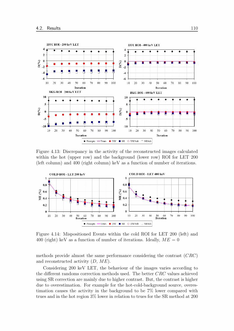
4.2. Results 110
Figure 4.13: Discrepancy in the activity of the reconstructed images calculatedwithin the hot (upper row) and the background (lower row) ROI for LET 200(left column) and 400 (right column) keV as a function of number of iterations.
Figure 4.14: Mispositioned Events within the cold ROI for LET 200 (left) and400 (right) keV as a function of number of iterations. Ideally, ME = 0
methods provide almost the same performance considering the contrast (CRC)and reconstructed activity (D, ME).
Considering 200 keV LET, the behaviour of the images varies according tothe different randoms correction methods used. The better CRC values achievedusing SR correction are mainly due to higher contrast. But, the contrast is higherdue to overestimation. For example for the hot-cold-background source, overes-timation causes the activity in the background to be 7% lower compared withtrues and in the hot region 3% lower in relation to trues for the SR method at 200
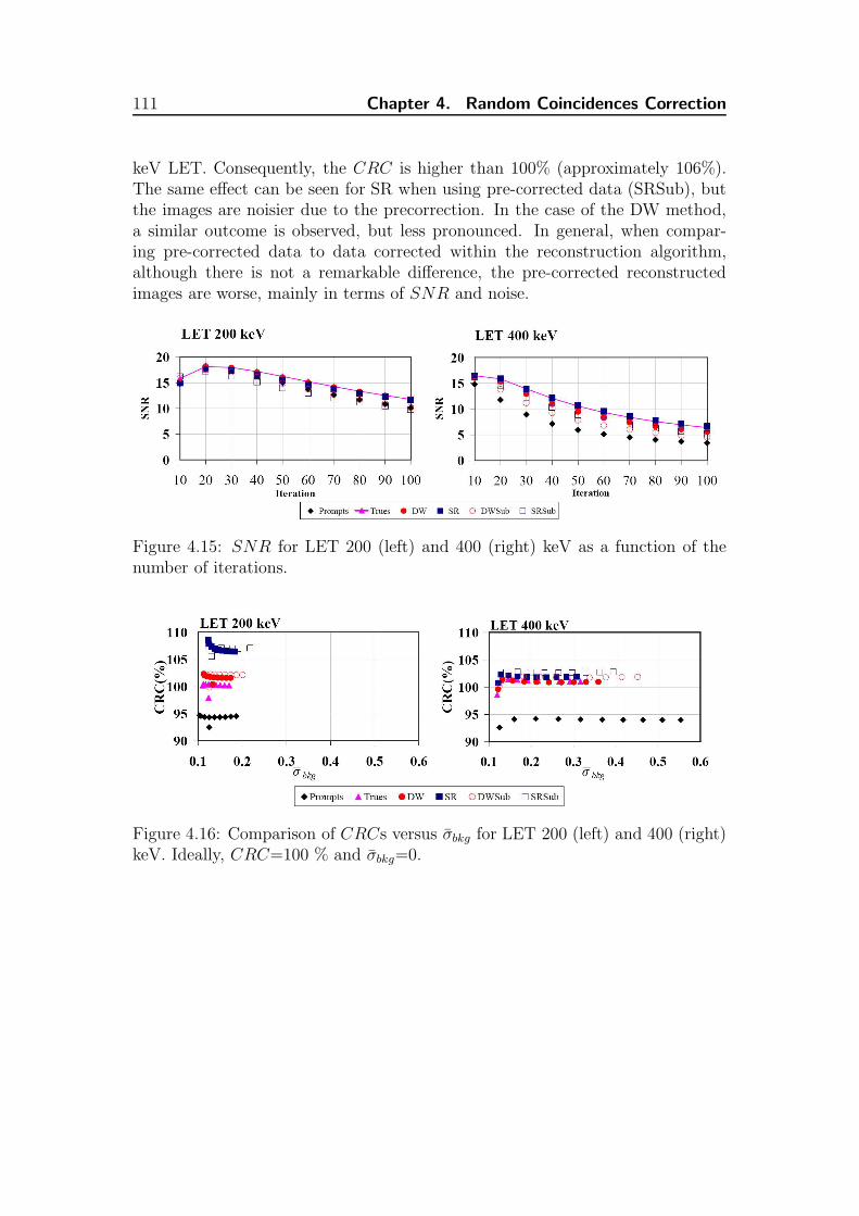
111 Chapter 4. Random Coincidences Correction
keV LET. Consequently, the CRC is higher than 100% (approximately 106%).The same effect can be seen for SR when using pre-corrected data (SRSub), butthe images are noisier due to the precorrection. In the case of the DW method,a similar outcome is observed, but less pronounced. In general, when compar-ing pre-corrected data to data corrected within the reconstruction algorithm,although there is not a remarkable difference, the pre-corrected reconstructedimages are worse, mainly in terms of SNR and noise.
Figure 4.15: SNR for LET 200 (left) and 400 (right) keV as a function of thenumber of iterations.
Figure 4.16: Comparison of CRCs versus σbkg for LET 200 (left) and 400 (right)keV. Ideally, CRC=100 % and σbkg=0.

4.2. Results 112
4.2.5 Effect of the activity on the overestimation of ran-doms
In this section we discuss the dependence of the overestimation of randoms onthe source activity. For this part, we have focused on one source, the hot-cold-background, two LETs (200 and 400 keV) and two random estimation methods,SR and DW. To run all the simulations in a feasible time, the acquisition time inthe simulation has been reduced to compensate the increase of activity, keepingthe number of emitted events and the simulation time4 constant. The results areshown in figure 4.17. As we can see from the figure 4.17, the randoms overesti-mation in the case of the DW is constant with the activity, whereas in the caseof the SR increases notably. The probability of having triple (and also multiples)random coincidences goes up as the activity raises, although these triple randomare considered negligible to develop the expression used in the SR method [104].At 400 keV LET, the triple randoms represent 1% of the sum of double andtriple coincidences when the activity of the background is 3.7 MBq, whereas at74 MBq background activity, the percentage of triple randoms over the sum oftriples and doubles is 12%. In the case of 200 keV LET, the ratios between triplerandoms and the sum of triple and double coincidendes are 3% and 25% for 3.7and 74 MBq of background activity, respectively. Therefore, these triple randomcoincidences, present in both 200 and 400 keV LETs, produce the increase of theoverestimation for higher activities in the SR method.
Figure 4.17: Ratio between dr estimated with DW and SR methods and dr ob-tained using GATE information for the hot-cold-background source and for thedifferent activities (τ=20 ns).
Next we consider the effect of the activity in the randoms corrected images.We have selected three reference values among those shown in the figure 4.17.These correspond to a total activity of the background region of 11.1, 27.75and 74 MBq. The reconstructed images for these activities can be seen in thefigures 4.18 for the 200 keV LET case, and 4.19 for the 400 keV LET. The first
4The time that the simulation is running on the computer.
113 Chapter 4. Random Coincidences Correction
interesting feature of these images is that, as a consequence of not correctingfor randoms (first column: prompts), there are artifacts in the image, not onlythe high intensity voxels at the edge of the FOV, but also a ring-flower likestructure inside of the hot-cold-background phantom. This structure is similarto a reconstructed image where all the LORs have the same value (figure 4.20b).The random coincidences add background noise in the data and thus, the useof the constant LOR histogram. The artifact becomes more important as theactivity increases, because the random coincidences rate increases as the squareof the activity. For the trues reconstructed images (second column of figures 4.18and 4.19), slight differences between them are noticeable. These differences aredue to the less statistics in the input data as the activity increases (see table 4.3and 4.5). The original double trues at lower activities may become triple randomsat higher activities, thus the reduction in double trues as the activity increases.Also it can be seen that the images at 400 keV are noisier than the others at 200keV, as a consequence of the lower sensitivity at this LET.
For the DW reconstructed images (third column of both figure 4.18 and 4.19),those with 74 MBq of background activity and both LETs show blurred edges ofthe background, hot and cold regions. This is more obvious for the case at 200keV LET than at 400 keV. The plots in figure 4.17 show that the overestimationof the DW method is almost constant with the activity for both LETs. Therefore,one could expect that the overestimation has the same effect on the images at 74MBq than at 3.7 MBq. But, due to the fact that the random coincidences increaseas the square of the activity, the outcome of the overestimation is higher for higheractivities, as we can see in tables 4.2 and 4.4 in the percentage of the randoms forthe DW method. This is the reason of the lowest quality of the DW-images at 74MBq. Looking at the table 4.3, one can see that the dgate
t at 74 MBq is slightlylower than the dDW
t at 27.75 MBq, and observing the reconstructed images thereare some differences in them. The edges of the phantom structure are blurrier inthe case of DW method and 27.75 MBq. Thus, the overestimation for the DWat 27.75 MBq is removing important information for the reconstruction and it isaffecting to the quality of the reconstructed image (it is more obvious the caseof SR method at 11.1 MBq, that has almost the same trues than the simulation,dgate
t , at 74 MBq, but the SR reconstructed image is worse).
Finally, the reconstructed images corrected using the SR estimation (fourthcolumn) are strongly affected by the overestimation, up to the point that thesource cannot be properly reconstructed, as it is the case for the backgroundactivity of 27.75 and 74 MBq at 200 keV LET and 74 MBq at 400 keV LET.Indeed the SR corrected image for 74 MBq at 200 keV LET shown in figure 4.18corresponds to the 20th iteration; further iterations lead to an image in whichall the voxels have zero intensity. Thus for the SR method, the combination ofthe increase of both the overestimation and the random coincidences with theactivity produces poorly reconstructed images.
After the qualitative analysis of the reconstructed images, we present relevantFOMs for these corrected images. In the figure 4.21, the plots of the discrepancyversus the iteration number for the DW corrected images are shown. At 200 keV
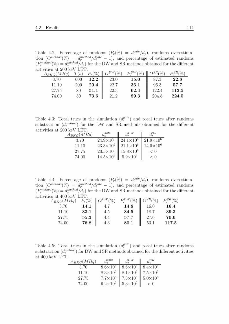
4.2. Results 114
Table 4.2: Percentage of randoms (Pr(%) = dgater /dp), randoms overestima-
tion (Omethod(%) = dmethodr /dgate
r − 1), and percentage of estimated randoms(P method
r (%) = dmethodr /dp) for the DW and SR methods obtained for the different
activities at 200 keV LET.ABKG(MBq) T (s) Pr(%) ODW (%) P DW
r (%) OSR(%) P SRr (%)
3.70 600 12.2 23.0 15.0 87.3 22.811.10 200 29.4 22.7 36.1 96.3 57.727.75 80 51.1 22.3 62.4 122.4 113.574.00 30 73.6 21.2 89.3 204.8 224.5
Table 4.3: Total trues in the simulation (dgatet ) and total trues after randoms
substraction (dmethodt ) for the DW and SR methods obtained for the different
activities at 200 keV LET.ABKG(MBq) dgate
t dDWt dSR
t
3.70 24.9×10⁶ 24.1×10⁶ 21.9×10⁶
11.10 23.3×10⁶ 21.1×10⁶ 14.0×10⁶
27.75 20.5×10⁶ 15.8×10⁶ < 074.00 14.5×10⁶ 5.9×10⁶ < 0
Table 4.4: Percentage of randoms (Pr(%) = dgater /dp), randoms overestima-
tion (Omethod(%) = dmethodr /dgate
r − 1), and percentage of estimated randoms(P method
r (%) = dmethodr /dp) for the DW and SR methods obtained for the different
activities at 400 keV LET.ABKG(MBq) Pr(%) ODW (%) P DW
r (%) OSR(%) P SRr (%)
3.70 14.1 4.7 14.8 16.0 16.411.10 33.1 4.5 34.5 18.7 39.327.75 55.3 4.4 57.7 27.6 70.674.00 76.8 4.3 80.1 53.1 117.5
Table 4.5: Total trues in the simulation (dgatet ) and total trues after randoms
substraction (dmethodt ) for DW and SR methods obtained for the different activities
at 400 keV LET.ABKG(MBq) dgate
t dDWt dSR
t
3.70 8.6×10⁶ 8.6×10⁶ 8.4×10⁶
11.10 8.3×10⁶ 8.1×10⁶ 7.5×10⁶
27.75 7.7×10⁶ 7.3×10⁶ 5.0×10⁶
74.00 6.2×10⁶ 5.3×10⁶ < 0

115 Chapter 4. Random Coincidences Correction
(a) Prompts (b) Trues (c) DW (d) SR
Figure 4.18: Reconstructed images of the hot-cold-background phantom, using100 iterations of MLEM, and at 200 keV LET for different activities: First rowcorrespond to ABKG = 11.1 MBq; Second row, ABKG = 27.75 MBq; Third row,ABKG = 74 MBq. The SR corrected image for 74 MBq corresponds to the 20thiteration, because the image of the 100th iteration has value zero for all the voxels.
LET (two most left plots), it is observed that, although the overestimation inthe DW method is almost independent of the activity, the discrepancy is nega-tively increasing with the activity due to the higher percentage of the randomcoincidences. As we have seen before, the overestimation affects more to thebackground region than to the hot one. From figure 4.17 we know that the over-estimation is around 5-4% for the DW method at 400 keV LET, and we hardlysee an effect in the reconstructed images, except for the images with backgroundactivity of 74 MBq, where we found the biggest difference between the randomspercentage, Pr, and the estimated randoms percentage for DW method, P DW
r
(see table 4.4).
In the case of the SR method, the plots of the discrepancy for the hot andbackground ROIs are displayed in the figure 4.22. The behaviour observed inthese plots is expected from the increase of the overestimation and the poorquality of the reconstructed images as the activity increases. In the SR method,an increase in the activity yields an increment of the overestimation for bothLETs (increase of the triple coincidences that are not accounted for in the SR

4.2. Results 116
(a) Prompts (b) Trues (c) DW (d) SR
Figure 4.19: Reconstructed images of the hot-cold-background phantom, using100 iterations of MLEM, and a 400 keV LET for different activities: First rowcorrespond to ABKG = 11.1 MBq; Second row, ABKG = 27.75 MBq; Third row,ABKG = 74 MBq
(a) Prompts (b) Constant LOR his-togram
(c) Combination ofboth images
Figure 4.20: (a) Reconstructed image of the hot-cold-background phantom, using100 iterations of MLEM, and a 200 keV LET for a background activity of 74 MBq.(b) Reconstructed image of a uniform LOR histogram after 100 iterations and at200 keV LET. (c) Superposition of the previous images.
expression). This increment together with the higher randoms percentage leadsto a poor quantification of the hot and background ROIs, being worse for thebackground and for the 200 keV LET. The discrepancy values of the reconstructed

117 Chapter 4. Random Coincidences Correction
0 20 40 60 80 100
-40
-30
-20
-10
0
DH
OT(%
)
Iteration
ABKG
= 3.7 MBq A
BKG = 11.1 MBq
ABKG
= 27.75 MBq A
BKG = 74 MBq
DW - LET = 200 keV
0 20 40 60 80 100-25
-20-15
-10-5
0
DH
OT(%
)
Iteration
ABKG
= 3.7 MBq A
BKG = 11.1 MBq
ABKG
= 27.75 MBq A
BKG = 74 MBq
DW - LET = 400 keV
0 20 40 60 80 100
-40
-30
-20
-10
0
ABKG
= 3.7 MBq A
BKG = 11.1 MBq
ABKG
= 27.75 MBq A
BKG = 74 MBq
DB
KG(%
)
Iteration
DW - LET = 200 keV
0 20 40 60 80 100-14-12-10-8-6-4-20
ABKG
= 27.75 MBq A
BKG = 74 MBq
ABKG
= 11.1 MBq A
BKG = 3.7 MBq
DB
KG(%
)
Iteration
DW - LET = 400 keV
Figure 4.21: Discrepancy of the hot (top row) and background (down) ROI forthe DW method and both LETs (200 keV at the left column and 400 keV at theright one) plotted versus the iteration number.
images of the 74 MBq background activity at 200 keV for both ROIs were notplotted because all the images were zero after the 20th iteration.
To end up with the part of the analysis for different activities, the CRC ver-sus the normalized background noise for these images is given in figure 4.23. Themain effect of the overestimation is to increase the CRC, as it was also observedin figure 4.16. In the case of 400 keV LET and the DW method, since the overes-timation is very small and almost constant, the CRC is close to 100% for all thestudied activities, except for the highest one where the randoms overestimationproduce the highest increment in the random percentage. When the LET is 200keV for the corrected images using the DW method, the CRC is above 100 % forall the activities, due to the fact that the overestimation is higher as comparedto the one at 400 keV LET. In the same way, for the SR method and both LETs,as the overestimation is higher than in the DW method and going up with theactivity, the CRC is always higher than 100 %, even for the lowest activity and400 keV. In the SR method, for the activities 27.75 MBq and 74 MBq at 200 keVLET the CRCs is above 300 % and it has not been plotted. The same happens at400 keV LET and SR method, but only for the background activity of 74 MBq.

4.3. Conclusions 118
0 20 40 60 80 100-70-60-50-40-30-20-100
DH
OT(%
)
Iteration
ABKG
= 3.7 MBq A
BKG = 11.1 MBq
ABKG
= 27.75 MBq
SR - LET = 200 keV
0 20 40 60 80 100-80-70-60-50-40-30-20-100
ABKG
= 3.7 MBq A
BKG = 11.1 MBq
ABKG
= 27.75 MBq A
BKG = 74 MBq
DH
OT(%
)
Iteration
SR - LET = 400 keV
0 20 40 60 80 100-100
-80
-60
-40
-20
0
ABKG
= 3.7 MBq A
BKG = 11.1 MBq
ABKG
= 27.75 MBq
DB
KG(%
)
Iteration
SR - LET = 200 keV
0 20 40 60 80 100
-100-80-60-40-200
ABKG
= 3.7 MBq A
BKG = 11.1 MBq
ABKG
= 27.75 MBq A
BKG = 74 MBq
DB
KG(%
)
Iteration
SR - LET = 400 keV
Figure 4.22: Discrepancy of the hot (top row) and background (down) ROI forthe SR method and both LETs (200 keV at the left column and 400 keV at theright one) plotted versus the iteration number.
4.3 Conclusions
Delayed window and singles rate methods have been used in this chapter to esti-mate the random coincidences for MADPET-II at various low energy thresholds.For LETs lower than 255 keV, a notable overestimation of the random coinci-dences is observed, being higher for the SR method than for the DW method.The overestimation found in the DW and DW’ methods cannot be explained fromthe chosen delay. It was found that this overestimation is mainly caused by inter-crystal scatter, which plays an important role at these LETs. These results werepresented for a total activity of 3.7 MBq. When increasing the source activities,the overestimation goes up for the SR method, while it remains constant for theDW method. This behaviour of the SR method is explained by the incrementin the number of triple random coincidences. Images obtained by compensatingfor randoms in the reconstruction algorithm were in general improved in termsof SNR, noise levels and in the determination of the absolute activities than theimages made with pre-corrected data. Only in the ME, the pre-corrected imagesshow better results. In general, for all the LETs studied, the DW method is
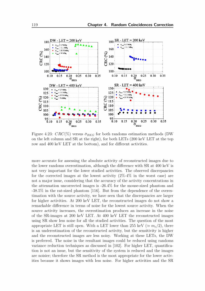
119 Chapter 4. Random Coincidences Correction
Figure 4.23: CRC(%) versus σBKG for both randoms estimation methods (DWon the left column and SR at the right), for both LETs (200 keV LET at the toprow and 400 keV LET at the bottom), and for different activities.
more accurate for assessing the absolute activity of reconstructed images due tothe lower randoms overestimation, although the difference with SR at 400 keV isnot very important for the lower studied activities. The observed discrepanciesfor the corrected images at the lowest activity (2%-4% in the worst case) arenot a major issue, considering that the accuracy of the activity concentrations inthe attenuation uncorrected images is -26.4% for the mouse-sized phantom and-38.5% in the rat-sized phantom [116]. But from the dependence of the overes-timation with the source activity, we have seen that the discrepancies are largerfor higher activities. At 200 keV LET, the reconstructed images do not show aremarkable difference in terms of noise for the lowest source activity. When thesource activity increases, the overestimation produces an increase in the noiseof the SR-images at 200 keV LET. At 400 keV LET the reconstructed imagesusing SR show less noise for all the studied activities. The question of the mostappropriate LET is still open. With a LET lower than 255 keV (≃ me/2), thereis an underestimation of the reconstructed activity, but the sensitivity is higherand the reconstructed images are less noisy. Working at these LETs, the DWis preferred. The noise in the resultant images could be reduced using randomsvariance reduction techniques as discussed in [102]. For higher LET, quantifica-tion is not an issue, but the sensitivity of the system is reduced and the imagesare noisier; therefore the SR method is the most appropriate for the lower activ-ities because it shows images with less noise. For higher activities and the SR

4.3. Conclusions 120
method, the overestimation has a higher effect on the reconstructed images and,as a consequence, must be corrected for. Future work should investigate howthe overestimation in the number of estimated randoms can be corrected usingDW and SR methods. Although this study was performed using the MADPET-II geometry, the results are expected to be valid for other systems with finelygranulated crystals.

Chapter 5
Triple Coincidences
A triple coincidence can be produced when three singles are found in the sametime coincidence window. These three singles could come mainly from one an-nihilation or from two annihilation that occur simultaneously or within a veryshort time. In order to have three singles consequence of one annihilation, oneof the photons must suffer a Compton interaction and deposit its energy in twocrystals (IC scatter). If the system has the ability of differentiating these twodepositions (MADPET-II has it), it is possible to obtain a triple coincidence outof the annihilation into two photons. In this chapter, we are interested in thistype of triple coincidences and they will be presented in the next section. Inthe second type that we mentioned, the triple coincidence occurs when one ofthe photons from the two annihilations is not detected. Because this situationimplies two annihilations, this would be a triple random coincidence and theyshould be included as random coincidences. Other combinations with more thantwo annihilations can take place that lead to a triple random coincidences, theseare rare for the activities of this study and not considered here (0.5 % of thetriple coincidences are formed by three singles from three different annihilationsat 3.7 MBq and a LET of 200 keV). Finally, the positron annihilation into threephotons could also generate a triple coincidence. But this is very suppressed (theyield of the three photon is 0.5% in water [119]) and therefore not accounted inthis thesis.
The contribution of the triple coincidences consequence of IC scatter can beused to increase the system efficiency. But, when the primary path of IC scatteris not properly identified, the spatial resolution could worsen. Therefore, theseevents have been investigated previously by our group in [108]. In the referredpaper, it was found out that the combination of individual crystal readout, a lowenergy threshold and an appropriate recovery scheme, the system efficiency wasincreased without any major worsening of the spatial resolution when includingthese triple coincidences. There was no study of the triple random coincidences in[108] because GEANT-3 did not provide time information of the detection process,as it does GATE. In this chapter we resort to this kind of triple coincidences dueto the problem found on the random coincidences estimation methods, moreimportant at lower LETs. As it was pointed out in the previous chapter (section
121

5.1. Triple Coincidences in MADPET-II 122
4.2.3), the combination of double and triple random coincidences for the DWmethod leads to a better estimation.
The goal of this part is to include the triple coincidences in the randomsestimation methods and in the image reconstruction process and determine if thetriple events, when working a lower LETs, solve the overestimation problem andproduce images with higher quality.
5.1 Triple Coincidences in MADPET-II
As we have already seen in the section 2.2 (page 72), triple true coincidences (sameannihilation process) can be detected by MADPET-II. This type of events takesplace when one of the annihilation photons delivers its energy in two crystals,whereas the other photon interacts only with one crystal (figure 2.5).
One of the question that arises when handling with triple coincidences is whichis, among all possibles LORs, the one related to the original trajectory. To iden-tify the right LOR is important to minimize the spatial resolution degradation.Several algorithms were proposed and studied to identify the primary path ofthe IC scatter event and then, take the corresponding LOR in [118], [120], [121],[122], [123], [108], [124], [125], [126], [127] and [128]. From the proposed identi-fication algorithms, we have used in this work the Maximum Energy algorithm(ME). Although this algorithm has not the highest identification fraction (IF), itis easy to implement and shows less dependence with the energy resolution.
The first step when working with triple coincidences is to differentiate betweenthe two singles related to the IC scatter event and the single related to the non-scattered photon (or, at least, the photon that has generated only one single)using a geometrical condition. We named the last one reference single. Thesecond step is to apply the ME algorithm to the two singles that belong to the ICscatter. The crystal of the single that has delivered the highest energy is taken incombination with the crystal of the reference single to form the LOR. An schemaof these two steps can be seen in figure 5.1.
5.2 System Matrix for the triple coincidences
The purpose of this chapter is to include the triple coincidences in the imagereconstruction process, in the frame of a iterative reconstruction algorithm (incontrast to [108] where an analytic framework was used). Therefore, a systemmatrix that accounts for this kind of coincidences should be built by using MonteCarlo techniques, continuing with our approach. As we mentioned in chapter 3,computing a 3D system matrix (even employing symmetries and distributed com-puting) would take several months. Especially if triple coincidences are taken intoaccount, due to the number of possible combinations. For this reason, generatinga 2D-system matrix (only for a transversal slice of the FOV, but the emission isin 3D) is a faster way to check, that the introduction of the triples coincidencesprovide reconstructed images with the same quality than without and improve

123 Chapter 5. Triple Coincidences
Figure 5.1: Different steps in the procedure of assigning LOR to a triple coinci-dence. After the triple coincidence is detected, the first step is to identify whichis the reference single and which are the IC scatter singles, by employing a ge-ometrical condition. In the second step, the most energetic single from the twosingles that were identified as IC scatter, is used in combination of the referencesingle to assign the LOR.
the results of the random coincidences corrected images. We use the prefix 2D inthe SM to highlight the fact that the SM is only for one transversal slice, althoughthe emission is in 3D and the complete scanner is employed for the detection.
A central plane of the FOV was chosen to create the SM for the triple coinci-dences (figure 5.2). We have used the simulations previously done for the chapter3. But we only employed the simulations of the voxels that belong to this cen-tral plane. The output files of these simulations were processed again, but in adifferent way: only triple true coincidences were considered (m = 2 and all thesingles had the same EventID) and the LOR was assigned using the ME algorithmexplained in the previous paragraph. After processing data in the simulations,the triple true coincidences in the LOR i coming from the voxel j, ctriples
ij , areobtained. It is possible to calculate the elements of the doubles and triples SM byadding these new counts, ctriples
ij , to the ones obtained for the double coincidencescase, cdoubles
ij .
For consistency with the previous chapters 3 and 4, we compare the SM, the

5.3. Random estimation method 124
70 mm 70 mm
0.5 mm
3D 2D
20 mm
Figure 5.2: As a proof-of-concept, the SM only for a central plane of the wholeFOV (2D) was taken to evaluate the inclusion of the triple coincidences.
randoms overestimation and the reconstructed images for the cases of doublecoincidences (P doubles) and double and triple coincidences (P dou+tri) at 200 keVLET.
5.3 Random estimation method
The DW and SR random estimation methods were modified to include the triplerandom coincidences, as we will explain in the next two sections.
5.3.1 Delayed Window method
Using this method, a triple random coincidence was considered when two singleswere found in the delayed window, as explained in chapter 4. In order to usethe estimation method to correct and reconstruct images, we need to define somecriteria to obtain the LOR for the estimated triple random coincidence. Wehave used either these two criteria to assign the corresponding LOR: maximumdistance (MD) and maximum energy (ME). The MD criterion calculates thedistance between the single that opens the time coincidence window and thetwo singles that are found in the delayed window. The combination of detectorsthat provides the maximum distance is the one taken to define the LOR. On theother hand, the ME criterion chooses the single among the two singles withinthe delayed window that has the highest energy deposition. As we are handlingwith random coincidences, there is no reason that supports one condition morethan the other. The criteria were applied to the two singles within the delayedwindow, and the single that opens the time coincidence window was consideredthe reference. The maximum distance condition uses the crystals combinationof the reference single with that single in the delayed window that yields thelongest LOR. The maximum energy criterium was applied to the two singles thatwere in the delayed window: to define the LOR, the highest energetic singlewithin the delayed window was combined with the reference single. The randomcoincidences estimated using MD or ME condition for the DW method will benamed as DWmd and DWme, respectively.
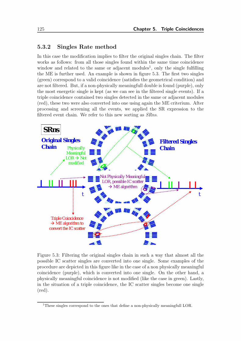
125 Chapter 5. Triple Coincidences
5.3.2 Singles Rate method
In this case the modification implies to filter the original singles chain. The filterworks as follows: from all those singles found within the same time coincidencewindow and related to the same or adjacent modules1, only the single fulfillingthe ME is further used. An example is shown in figure 5.3. The first two singles(green) correspond to a valid coincidence (satisfies the geometrical condition) andare not filtered. But, if a non-physically meaningfull double is found (purple), onlythe most energetic single is kept (as we can see in the filtered single events). If atriple coincidence contained two singles detected in the same or adjacent modules(red), these two were also converted into one using again the ME criterium. Afterprocessing and screening all the events, we applied the SR expression to thefiltered event chain. We refer to this new sorting as SRns.
Figure 5.3: Filtering the original singles chain in such a way that almost all thepossible IC scatter singles are converted into one single. Some examples of theprocedure are depicted in this figure like in the case of a non physically meaningfulcoincidence (purple), which is converted into one single. On the other hand, aphysically meaningful coincidence is not modified (like the case in green). Lastly,in the situation of a triple coincidence, the IC scatter singles become one single(red).
1These singles correspond to the ones that define a non-physically meaningfull LOR.

5.4. Simulated sources 126
5.4 Simulated sources
We want to address the following objectives with the simulated sources employedin this chapter:
• Evaluate the spatial resolution degradation when including the triple truecoincidences and the primary path recovery algorithm.
• Validate the modified DW and SR methods to compensate for triple randomcoincidences.
• Include the estimated triple random coincidences aimed at reducing theoverestimation and obtaining better agreement between the randoms cor-rected reconstructed images and the reconstructed images with true coin-cidences.
(a) (b) (c)
Figure 5.4: Various sources simulated with GATE to study the introduction oftriple coincidences in the image reconstruction process (see table 5.1 for sourcedimensions).
The simulated sources for this study (see figure 5.4) were confined to thetransversal plane in which the doubles and triples SMs was calculated. Thereforethe axial dimension of these sources was 0.5 mm to fit into the axial voxel size ofthe SMs.
Related to the spatial resolution degradation, we have used two sources: thehorizontal capillaries that cover the radial FOV and a Derenzo phantom (figures5.4a and 5.4b). The Derenzo-like phantom was used for qualitative analysis ofthe image. Like in the chapter 3, this phantom consists of 6 sectors. Each sectorcontains 0.5 mm long rod sources with diameters of 0.8, 1.0, 1.2, 1.6, 2.4 and3.2 mm and rod separation twice the diameter. The rod sources were spreadwithin a disc of 62 mm diameter. The total activity of this source was 22.2 MBq.The acquisition time of the simulation was 300 s (number of detected eventsfor doubles and doubles and triples). The horizontal capillaries were employedto assess quantitative values related to the spatial resolution. This source iscomposed of small cylindrical sources of 0.5 mm long and 0.25 mm radius. Theyare extended covering the radial FOV and the separation distance between themis 5 mm.

127 Chapter 5. Triple Coincidences
Table 5.1: Simulated sources used in this triple coincidences study.
Source Position Dimensions(mm) A(MBq)a Horizontal Radial FOV r = 0.25, h = 0.5 9.62
Capillaries dCap = 5b Derenzo centered r = 0.4, 0.5, 0.6, 0.8 22.2
r = 1.2, 1.6, h = 0.5c Hot-Cold-Bkg centered Cyl.:r = 30 3.7/1.59(3:1)
Rods: r = 10,h = 0.5
The second and third points of the previous list were studied simulating ahot-cold-background phantom. This phantom has the same structure than inchapters 3 and 4, excepting the axial dimension, which is reduced to 0.5 mm.
5.5 Figures of merit
The possible spatial degradation was studied calculating the FWHM and FWTM(characterized in section 1.1.4) of the line profiles of the reconstructed capillariesfor the true coincidences (double true coincidences in the case of Pdoubles, anddouble and triple trues for Pdou+tri). To see the effect on the quantification of theimages when adding the triple coincidences, the following figures-of-merit wereemployed (all of them defined in section 1.1.4, page 57):
1. Discrepancy (D), calculated using the hot and background ROIs defined infigure 3.5, but with the axial dimension set to 0.5 mm; the reference is thereconstructed image obtained employing only the true coincidences. Thereconstructed images with and without randoms correction are comparedto the reference.
2. Background Noise (σbkg)
3. Contrast Recovery Coefficient (CRC)
5.6 Results and Discussion
5.6.1 Characterization of System Matrices
The values presented in this section correspond to the SM related to the voxelsbelonging to a central slice of the FOV. Using these 2D-system matrices, the diskspace needed to store the SMs is not a problem. Therefore, the full SM (not 1/4of it) can be saved in a binary file that contains the values of the triplet voxel (j),LOR (i) and the corresponding counts for this combination of voxel-LOR, cij.The emitted gamma-ray pairs for this case were 30.760×10⁹ (2 million of 511 keVphoton pairs for each voxel, 15380 voxels belong to this FOV), the sum of the cij

5.6. Results and Discussion 128
Table 5.2: Properties of the calculated 2D probability matrices at 200 keV LET
Nnonzero σrel S Disk space(%) (%) (GB)
Doubles 159,699,164 0.84 1.50 1.8Doubles & Triples 187,994,856 0.84 1.80 2.2
coefficients for the case of the doubles at 200 keV (total detected photons pair)was 4.58×10⁸. When including the triple true coincidences (0.93×10⁸ detected at200 keV), the value of the sum was 5.51×10⁸ (20% more compare to only doubletrue coincidences). Considering the LORs that have non-zero counts, the averagenumber of counts per LOR was 829.395 for doubles only, whereas for doublesand triples the average increased to 994.806. The elements of the SM with onedetected event (cij = 1) was also higher when the triples were accounted for,1.09×108 compared to 1.30×10⁸. In both cases, it represented the 69% of thetotal of non-zero elements. The maximum (average) of the coefficients was 85(2.87) for the SM with doubles only and 91 (2.93) for doubles and triples.
The summary of the main properties of this special case of SMs is shown intable 5.2. In this table, it is observed that the statistical quality of both SMs isequal. This means that when including the triples, not only the maximum andaverage were increased, but also the number of non-normalized elements with onecount (indeed, the percentage of these elements is the same for both SM). As itwas expected, the sensitivity at 200 keV LET taking into account the triples ishigher than in the case of only doubles at the same LET.
In GATE there is no variable that informs about if the single was created fromone of the annihilation photon or the other. Therefore, when handling with triplecoincidences in GATE, it is not always possible to identify which is the referencesingle2. For this work, in order to decide which was the reference single we haveemployed a geometrical condition. This geometrical condition is supported by thefact that, for around 95% of the triple true coincidences, two of the three singlesare detected in the same (75-80%) or adjacent (20-14%) modules and a thirdsingle elsewhere. Therefore the geometrical condition to determine the referencesingle was the one that gave the most common combination when using tripletrue coincidences and the reference single was the third one (afterwards with thetwo closest detected singles the ME condition was applied). If the geometricalcondition was not satisfied, the two most energetic singles were chosen to assignthe LOR. The triple prompts were classified according to this schema. Althoughthe way we process the triples introduces some uncertainty, this degradationeffect is also taken into account in the SM. Therefore, the degradation will bepartially compensated during the reconstruction. Because the model is not perfect(statistical noise), the SM cannot remove completely the mispositioning.
We have also calculated the sensitivity matrix for these two cases. In figure
2The reference single can be distinguished only in the cases, in which it has undergone onlya photoelectric effect. In this cases, the ComptonCrystal variable is zero.

129 Chapter 5. Triple Coincidences
5.5 we observe the same structure of the sensitivity matrix for the doubles andtriples and for only the doubles at 200 keV. The main difference is the increase ofthe sensitivity when adding the triples. The increase of sensitivity when includingtriples is shown clearly in the profiles of figure 5.5. We have also calculated theratio of these matrices and, as expected, the values are in the range of [1.18,1.22].
(a) SDou (b) SDou+Tri
Figure 5.5: Top: Sensitivity Matrix of the central slice for the two studied cases.The one for the doubles is at the left (SDou) and the one for doubles and triplesis at the right (SDou+Tri). Bottom: Profiles of both sensitivity matrices (left) andratio of the two sensitivity matrices (right).
5.6.2 Effect on spatial resolution
In this section we examine if there is some degradation of the spatial resolution byincluding the triple coincidences. Besides, we are interested in the validation ofthe proposed schema for processing the IC scatter events. In figure 5.6, we presentthe reconstructed images of the Derenzo phantom for both cases, employing truecoincidences. We observe that, when adding the triple coincidences to the data,no degradation of the spatial resolution is visible. On the contrary, the rods of1.2 mm, which are not visible in the case of doubles, can be distinguished in theregion close to the center in the reconstructed image using doubles and triples.

5.6. Results and Discussion 130
These observations lead us to think that the increase of the sensitivity when usingthe triple coincidences together with the modelling of the uncertainty introducedby the recovery algorithm in the SM produce images with higher quality.
Figure 5.6: Reconstructed images of the Derenzo phantom after 100 iterationsfor the two system matrices and 200 keV LET (left: only doubles; right: doublesand triples).
The reconstructed horizontal capillaries have been used for determining thespatial resolution (figure 5.7). There is no important differences between thereconstructed images of the capillaries using the two SMs. In the figure 5.8 theline profiles of the images are shown. From these line profiles the FWHM andFWTM were calculated (figure 5.9). The value of the FWHM varies slightlyaround 1 mm within the 70% of the radial FOV for both SMs. The FWHMreaches its maximum, 1.12 mm at the position corresponding with the 85% of theFOV. A slight difference between the two images is found at the edges of the FOVand this difference can be quantified using the FWTM. Only the last capillary ofthe reconstructed image with triples has higher FWTM than the image obtainedonly with doubles. The rest of the capillaries, on the contrary, show a lowerFWTM in the case of doubles and triples than only doubles. In general, thisquantitative result supports the same reasoning that we got from the Derenzoimages: Not only there is no spatial degradation of the image when adding thetriples, but also the reconstructed images employing doubles and triples showbetter quality in terms of spatial resolution. And this improvement is due to ahigher sensitivity combined with modelling the recovery schema within the SM.
Figure 5.7: Reconstructed images of the capillaries extended through the radialFOV after 100 iterations for the different system matrices at 200 keV LET (left:only doubles; right: doubles and triples.)
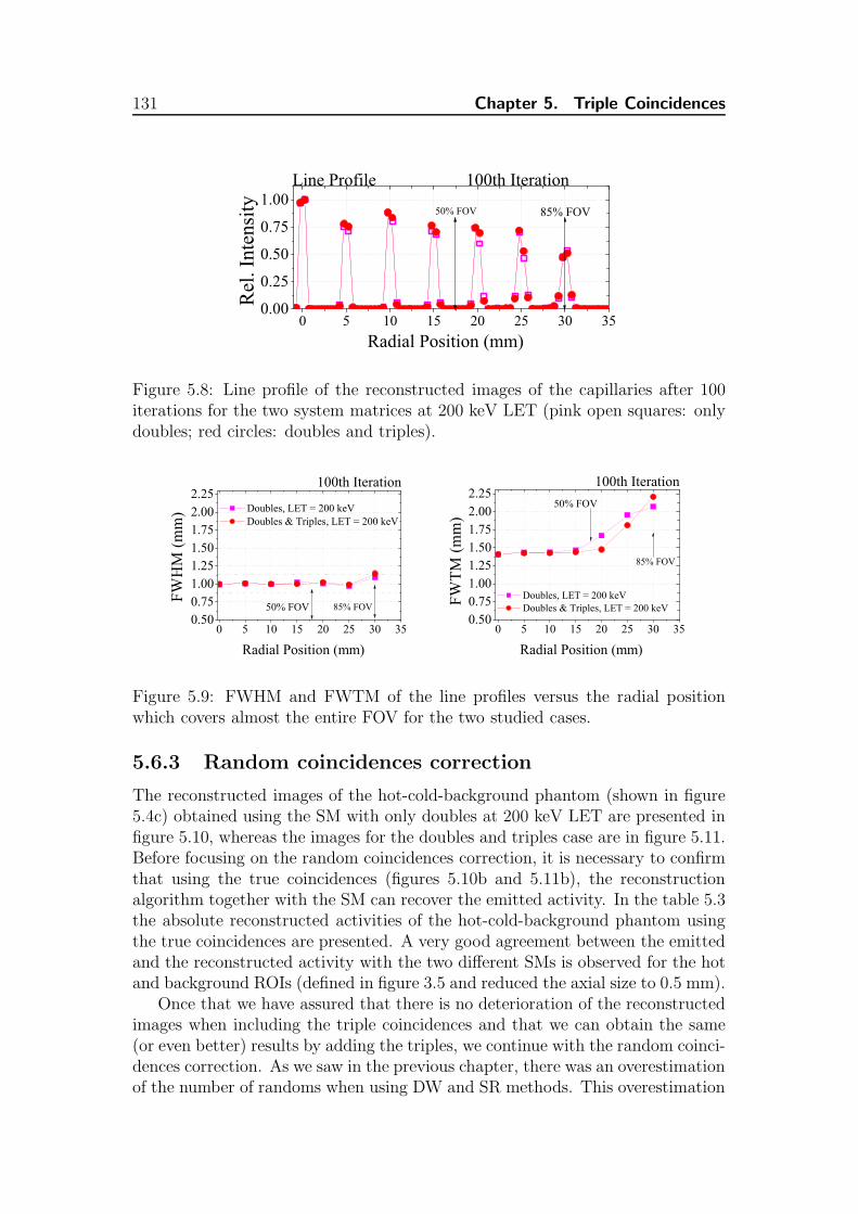
131 Chapter 5. Triple Coincidences
0 5 10 15 20 25 30 350.00
0.25
0.50
0.75
1.00 50% FOV
Rel
. Int
ensi
ty
Radial Position (mm)
85% FOV
100th IterationLine Profile
Figure 5.8: Line profile of the reconstructed images of the capillaries after 100iterations for the two system matrices at 200 keV LET (pink open squares: onlydoubles; red circles: doubles and triples).
0 5 10 15 20 25 30 350.500.751.001.251.501.752.002.25
50% FOV
FWH
M (m
m)
Radial Position (mm)
Doubles, LET = 200 keV Doubles & Triples, LET = 200 keV
85% FOV
100th Iteration
0 5 10 15 20 25 30 350.500.751.001.251.501.752.002.25
50% FOV
FWTM
(mm
)
Radial Position (mm)
Doubles, LET = 200 keV Doubles & Triples, LET = 200 keV
85% FOV
100th Iteration
Figure 5.9: FWHM and FWTM of the line profiles versus the radial positionwhich covers almost the entire FOV for the two studied cases.
5.6.3 Random coincidences correction
The reconstructed images of the hot-cold-background phantom (shown in figure5.4c) obtained using the SM with only doubles at 200 keV LET are presented infigure 5.10, whereas the images for the doubles and triples case are in figure 5.11.Before focusing on the random coincidences correction, it is necessary to confirmthat using the true coincidences (figures 5.10b and 5.11b), the reconstructionalgorithm together with the SM can recover the emitted activity. In the table 5.3the absolute reconstructed activities of the hot-cold-background phantom usingthe true coincidences are presented. A very good agreement between the emittedand the reconstructed activity with the two different SMs is observed for the hotand background ROIs (defined in figure 3.5 and reduced the axial size to 0.5 mm).
Once that we have assured that there is no deterioration of the reconstructedimages when including the triple coincidences and that we can obtain the same(or even better) results by adding the triples, we continue with the random coinci-dences correction. As we saw in the previous chapter, there was an overestimationof the number of randoms when using DW and SR methods. This overestimation
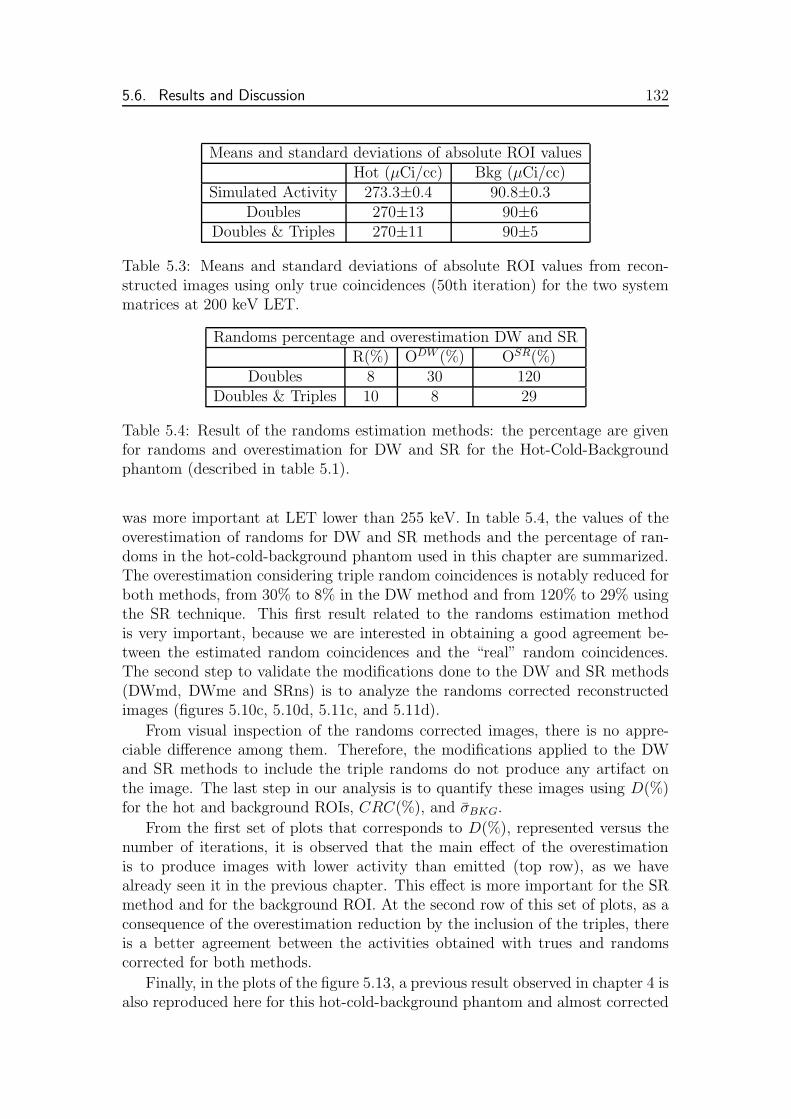
5.6. Results and Discussion 132
Means and standard deviations of absolute ROI valuesHot (µCi/cc) Bkg (µCi/cc)
Simulated Activity 273.3±0.4 90.8±0.3Doubles 270±13 90±6
Doubles & Triples 270±11 90±5
Table 5.3: Means and standard deviations of absolute ROI values from recon-structed images using only true coincidences (50th iteration) for the two systemmatrices at 200 keV LET.
Randoms percentage and overestimation DW and SRR(%) ODW (%) OSR(%)
Doubles 8 30 120Doubles & Triples 10 8 29
Table 5.4: Result of the randoms estimation methods: the percentage are givenfor randoms and overestimation for DW and SR for the Hot-Cold-Backgroundphantom (described in table 5.1).
was more important at LET lower than 255 keV. In table 5.4, the values of theoverestimation of randoms for DW and SR methods and the percentage of ran-doms in the hot-cold-background phantom used in this chapter are summarized.The overestimation considering triple random coincidences is notably reduced forboth methods, from 30% to 8% in the DW method and from 120% to 29% usingthe SR technique. This first result related to the randoms estimation methodis very important, because we are interested in obtaining a good agreement be-tween the estimated random coincidences and the “real” random coincidences.The second step to validate the modifications done to the DW and SR methods(DWmd, DWme and SRns) is to analyze the randoms corrected reconstructedimages (figures 5.10c, 5.10d, 5.11c, and 5.11d).
From visual inspection of the randoms corrected images, there is no appre-ciable difference among them. Therefore, the modifications applied to the DWand SR methods to include the triple randoms do not produce any artifact onthe image. The last step in our analysis is to quantify these images using D(%)for the hot and background ROIs, CRC(%), and σBKG.
From the first set of plots that corresponds to D(%), represented versus thenumber of iterations, it is observed that the main effect of the overestimationis to produce images with lower activity than emitted (top row), as we havealready seen it in the previous chapter. This effect is more important for the SRmethod and for the background ROI. At the second row of this set of plots, as aconsequence of the overestimation reduction by the inclusion of the triples, thereis a better agreement between the activities obtained with trues and randomscorrected for both methods.
Finally, in the plots of the figure 5.13, a previous result observed in chapter 4 isalso reproduced here for this hot-cold-background phantom and almost corrected

133 Chapter 5. Triple Coincidences
(a) Prompts (b) Trues (c) DW (d) SR
Figure 5.10: Reconstructed images of the Hot-Cold-Background phantom after50 iterations for the system matrix for doubles at 200 keV LET. (a) Prompts; (b)Trues; (c) Corrected for randoms estimated using DW method; (d) Corrected forrandoms estimated using SR method .
(a) Prompts (b) Trues (c) DWmd (d) SRns
Figure 5.11: Reconstructed images of the Hot-Cold-Background phantom after50 iterations for the system matrix for doubles and triples at 200 keV LET. (a)Prompts; (b) Trues; (c) Corrected for randoms estimated using DWmd method(There is no difference in the reconstructed images using DWmd and DWmemethods to estimate the triple randoms, therefore only the ones obtained withDWmd is presented); (d) Corrected for randoms estimated using SRns method .
when adding the triples. We refer to the fact that the CRC is higher than 100%due to the overestimation, this values are seen for the plot at the left. The highestvalue of the CRC is 105% and corresponds to the SR method. In the plot atthe right, where the triple coincidences are considered, the values of the CRC aregetting closer to 100% as one would expect. Another fact, consequence of thehigher sensitivity when taking into account the triple coincidences, is that thenoise is lower in these images.
5.7 Conclusions
The triple coincidences and their impact on the random coincidences methodshave been studied in this chapter. The benefit of taking into account thesetype of events for reconstruction is to increase the sensitivity of the system.Additionally, in the previous chapter we have found that using triple coincidencescould help us to solve the problem of the randoms overestimation. When including

5.7. Conclusions 134
10 20 30 40 50 60 70 80 90 100-6-4-202468
DB
KG(%
)
Iteration
Prompts Trues DW SR
Doubles, LET = 200 keV
10 20 30 40 50 60 70 80 90 100-5-4-3-2-1012345
DH
OT(%
)
Iteration
Prompts Trues DW SR
Doubles, LET = 200 keV
10 20 30 40 50 60 70 80 90 100-6-4-202468
DB
KG(%
)
Iteration
Prompts Trues DWmd DWme SRns
Doubles & Triples, LET = 200 keV
10 20 30 40 50 60 70 80 90 100-5-4-3-2-1012345
DH
OT(%
)
Iteration
Prompts Trues DWmd DWme SRns
Doubles & Triples, LET = 200 keV
Figure 5.12: Analysis of the hot and background ROIs of images reconstructedwith the two system matrices.
0.050 0.075 0.100 0.125 0.15096979899
100101102103104105
CR
C (%
)
BKG
Prompts Trues DW SR
Doubles, LET = 200 keV
0.050 0.075 0.100 0.125 0.15096979899
100101102103104105
CR
C (%
)
BKG
Prompts Trues DWmd DWme SRns
Doubles & Triples, LET = 200 keV
Figure 5.13: CRC versus the normalized standard deviation within the ROI in thebackground for randoms corrected and non-corrected images for the two studiedcases.
triple coincidences, it is necessary to know how to process them in order to notdeteriorate the quality of the reconstructed images.
First, we have confirmed that the sensitivity increases 20% at 200 keV LETwhen the triple coincidences are taken into account. Secondly, before startingwith the randoms coincidence correction, it was important to verify that thereis no degradation in the reconstructed images obtained using double and tripletrue coincidences. In order to do this, we have compared reconstructed imagesobtained with a SM that considers only double coincidences to a SM created withdouble and triple coincidences. In terms of spatial resolution, a Derenzo phantomand horizontal capillaries have been simulated and reconstructed with both SMs.

135 Chapter 5. Triple Coincidences
In the Derenzo images, we have found that not only there is no visual degradation,but also some rods of 1.2 mm close to the center, which were not visible for the SMwith doubles, are identified in the SM with doubles and triples. In the horizontalcapillaries, small differences are observed for the FWTM at the edges of the FOV.Additionally, the hot-cold-background phantom has been employed for testing thecapabilities of recovering the emitted activity. The reconstructed images withboth SMs are in good agreement to the emitted activity. Therefore, from thesefirst results obtained from true coincidences (doubles and triples), there is nodeterioration of the reconstructed images using doubles and triples. In additionwe can conclude that better quality in terms of spatial resolution is achievablewhen including the triple coincidences in the processing and reconstruction.
Related to the random coincidence correction, considering the triple events re-quires to modify the estimation method to include these events. We have adaptedDW and SR method and we have observed that, when including the triple ran-doms, the randoms overestimation (shown in the previous chapter) is notablyreduced. Additionally, the randoms corrected reconstructed images with triplesdo not show any artifact that would discourage us of using the modified randomestimation methods. On the contrary, there is no visual difference between themand the reconstructed images obtained with doubles only. From the quantitativeanalysis, we can infer that the introduction of the triples solves the underestima-tion of the activity and, due to the higher sensitivity, the noise in the images islower.
Therefore, triple events are good candidates to be included in the reconstruc-tion process, because not only increase the sensitivity of the system, but alsoreduce notably the randoms overestimation and improve the quantification of thereconstructed images at lower LET. Nevertheless, the approach presented in thischapter is a proof-of-concept, because all the results given here are for a 2D sys-tem matrix. Future work will be to confirm them with a 3D system matrix andlarger objects.
Lastly, for this work we have only focus in a sorting algorithm that uses asingle time coincidence window. Whereas there are other sorting algorithms thatemploys multiple time coincidence window. For further analysis on this issue werefer to [129], where a comparison between single and multiple time coincidencewindow sorting algorithms is done.

Chapter 6
Normalization Correction
The normalization correction in Positron Emission Tomography is necessary toobtain reconstructed images without artifacts and to assure proportionality be-tween the intensity of the reconstructed image and the emitted activity (section1.1.3, page 52). This correction depends on the algorithm employed for image re-construction. In the case of analytical reconstruction, the algorithm requires thatall the lines of response have the same sensitivity. In general this is not the case,there are geometric variations over the field of view and random and systematicvariations in individual detector efficiencies. The normalization factors can beassessed by irradiating all the detectors with a known activity source. The ratiobetween the detected coincidences in each detector and the expected coincidences(if all the detectors would have efficiency equal to 1) provides the normalizationfactors. This technique is known as direct normalization and its accuracy is lim-ited by the counts measured in the detectors, consequently by the time used tomake the normalization measurement. Another technique was proposed in [117],in which the normalization factor for a LOR can be derived from the product ofthe efficiencies of the detectors that define this LOR. By doing this, the numberof parameters to estimate is notably reduced, improving the statistical accuracyof the method. The authors present as well a variance reduction technique forcomputing the values of the efficiencies. Later on, in [131], a geometrical compo-nent was added to the previous model. In [133] the method was extended to fully3D scanners and the authors developed an algorithm using the geometric meanto obtain the detector efficiencies and geometrical factors. All these methods areknown as component-based normalization, to distinguish them from the directnormalization. When operating the PET scanner in 3D mode, object scatter in-creases notably and this situation must be taken into account when calculatingthe normalization factors. The latter has been addressed in [137], where a methodto calculate the normalization factors for trues and scattered coincidences is de-veloped. A more sophisticated component-based model can be found in [139],where the normalization coefficients are split into several factors which not onlyinvolve the crystal efficiencies and the geometry, but also the block profile andthe crystal interference pattern. An extension of this model to include the timealignment factors and count-rate dependence was presented in [141]. All the ref-
137

6.1. Normalization for to MADPET-II 138
erences presented up to this point apply the component-based approach to correctfor efficiency inhomogeneities (normalize) in the case of analytical algorithms. Inthe framework of statistical image reconstruction, the normalization correctiondepends on the model or method used to generate the system matrix, and thenormalization factors must account only for the effects that are not included inthe system matrix and produce variations in the sensitivity of the LORs [142].The component-based model can also be used in the statistical framework to cal-culate the normalization factors. This is the approach that we will apply in thischapter, and several methods to assess these factors will be analyzed.
6.1 Normalization for to MADPET-II
In this work, the MLEM algorithm combined with a Monte Carlo systemmatrix is used to reconstruct images for MADPET-II. All the geometrical factorsare included in the Monte Carlo SM; therefore, when using the component-basedmodel for normalization, only the detection efficiency of the LOR (εLOR) must beassessed. It is necessary to perform a measurement with the system in order toobtain the LOR efficiencies, called normalization measurement. We will describehow to estimate εLOR using a priori information from a Monte Carlo simulationcombined with the normalization measurement. The first approach calculates thenormalization factors using the coincidences in the normalization measurement.As in the direct normalization, when estimating the correction factors throughcoincidence measurements, the accuracy of the factors is limited by the numberof coincidences. In order to improve the statistical quality of the normalizationfactors, we propose a second method to calculate them where singles instead ofcoincidences from the normalization measurement are used. Under the assump-tion that the component-based model is valid, we can split the efficiency of aLOR into two factors –the two individual efficiencies of the crystals that definethe LOR (εcrystal)–, and we can employ singles measurements to obtain these in-dividual efficiencies. These two methods (coincidences-based and singles-based)will be applied to reconstruct images of MADPET-II and the validity of theseapproaches for the complete scanner will be investigated in a future work. Forthis chapter, we have tested these two approaches in the incomplete 384-channelprototype (see images in figure 6.2). When studying the effect of these normaliza-tion methods on the image reconstruction, it was necessary to rotate the sourceduring the data acquisition to compensate for the missing angular sampling ofthe non-present channels.
6.1.1 Calculation of the normalization factors
The normalization factors are coefficients which are applied to the input data(sinogram or LOR histogram) to provide the mentioned correction. In the directnormalization, they are proportional to the reciprocal of the number of countsobtained in each sinogram element or LOR in the normalization measurement. In

139 Chapter 6. Normalization Correction
this work, we use the following convention (similar to the direct normalization):we call normalization factors (NFi) to the values that multiply the input dataand efficiencies (εi) to the inverse of these factors (εi = 1/NFi). The efficienciesmodify the system matrix to account for normalization. Next we explain thecalculation of the LOR efficiencies employing the two proposed methods, singles-based and coincidences-based.
Singles data: Crystal efficiencies
The singles list data from the simulation and measurement were histogrammedaccording to the different detectors after applying the low energy threshold of400 keV. After analyzing the singles histograms, it was found that some of thedetector crystals had no counts at all or very few in the measurements. Thosedetector crystals that have no counts are called dead channels (or dead crystals).On the other hand, when there are only few counts (less than 50% of the countsfor the same channel in the simulation), we refer to it as a low efficiency crystal.Once the histograms for the measurement and for the simulations were done, thecrystal efficiency factors were calculated as follows:
εsink =
smeask /
∑
j smeasj
ssimk /
∑
j ssimj
, (6.1)
where k indicates the crystal number and runs from 0 to 1151, smeask is the
number of singles for the crystal k in the measurement, and ssimk is the number
of singles for the crystal k in the simulation. From the previous expression thecorresponding LOR efficiency was obtained as:
εsini(k,l) = εsin
k εsinl . (6.2)
Coincidences data: LOR efficiencies
The coincidences are obtained by sorting the singles in the same way for simu-lated and measured data, as it was explained in section 2.2 (page 70). The delayedwindow method is applied to eliminate the random coincidences in the measure-ments. When handling the simulated data, no randoms estimation method wasused, because it is possible to distinguish between true and random coincidencesfrom the information provided by the simulation program. The LOR efficienciesthen read:
εcoini(k,l) =
nmeasi /
∑
j nmeasj
nsimi /
∑
j nsimj
, (6.3)
where i(k, l) refers to the LOR i defined by the crystals k and l. nmeasi and nsim
i
are the number of coincidences in LOR i for the measurement and simulation,respectively.

6.1. Normalization for to MADPET-II 140
6.1.2 How to apply the normalization
The calculated normalization factors can be applied directly to the input file ofthe reconstruction program, which is a LOR histogram, just by multiplying thesefactors by the number of the coincidences measured in each LOR. We refer tothis method as direct normalization (DN).
A second approach is to modify the system matrix that is used in the MLEMalgorithm by the efficiencies (εi). The resulting system matrix would contain theinformation of the detector efficiency: the MCSM elements, pij, are multipliedby the efficiencies (pij = εipij) and the new elements of the MCSM, pij , take intoacount the efficiencies of the LORs. The effect of this modification in the MLEMalgorithm is:
f(n)j =
f(n−1)j
∑
i pij
∑
i
di∑
k pikf(n−1)k
pij =f
(n−1)j
∑
i εipij
∑
i
di∑
k εipikf(n−1)k
εipij . (6.4)
We see that the efficiencies in the second factor are cancelled out, and theefficiencies only modify the sensitivity matrix1:
f(n)j =
f(n−1)j
∑
i εipij
∑
i
di∑
k pikf(n−1)k
pij. (6.5)
In order to liken the two approaches, we show in the next expression the re-sulting equation from applying directly the normalization factors (DN approach):
f(n)j =
f(n−1)j
∑
i pij
∑
i
NFidi∑
k pikf(n−1)k
pij =f
(n−1)j
∑
i pij
∑
i
di
εi
∑
k pikf(n−1)k
pij (6.6)
Comparing the expression in 6.5 to 6.6, it is obvious that the correction inboth approaches acts differently.
To study the effect of the normalization, images were reconstructed in thefollowing cases combining the two above explained approaches and the two waysof calculating the normalization factors (singles-based and coincidences-based):
1. No normalization is applied (NN).
2. Direct normalization with factors calculated from singles (DN-S).
3. Direct normalization using factors obtained from coincidence events (DN-C).
4. Normalization within the reconstruction algorithm operating with the co-efficients from the singles, εsin
i(k,l) (NRI-S).
1This is only possible when neither the random coincidences, nor scatter coincidences arecorrected within the reconstruction algorithm

141 Chapter 6. Normalization Correction
5. Normalization within the reconstruction algorithm employing the correctioncoefficients from the coincidences, εcoin
i(k,l) (NRI-C).
Additionally, in the NRI-S and NRI-C cases, we have explored the feasibilityof reducing the scanning time by using a small part of the singles data streamfor the NRI-S and of the coincidences for the NRI-C. In the case of the singlesdata, the normalization factors have been calculated using only 1/12 of the totalsingles. This approach was named NRI-SLS, where the acronym LS refers to thelower statistic employed to assess the normalization factors. The coincidencesused for this lower statistic version NRI-CLS were 1/3 of the total coincidences.For all the studied cases for normalization, we have focused on data at 400 keVLET.
6.1.3 Normalization source
Different sources have been employed in the literature to calculate the normaliza-tion factors: In the case of 3D acquisitions [134] used a 68Ge plane source, [135]a uniform 20 cm cylinder (commonly consisting of 68Ge), [136] 68Ge transmissionscanning rod sources, and [143] a line source of 68Ge which oscillates across thetransaxial and an annular source. The advantages and disadvantages of usingthese different geometries have been shortly described in the introduction (sec-tion 1.1.3, page 52) and further details can be found in the references above (seealso [130]).
For the case of MADPET-II, we have used an aqueous flood source containedin a plastic cover to generate a low-scatter planar distribution of activity thatirradiates uniformly all the channels. The main two reasons of using this sourceare, on one hand, the presence of scatter is reduced notably in comparison to acylindrical source. On the other hand, the different source activities viewed byeach pair of detectors are more uniform in the case of the flood source than inthe cylindrical source (see figure 6.1). This leads to a similar statistical qualityof the normalization factors in the case of the flood source.
Measurement
The dimensions of the flood source are 1×40×25 mm3 and those of the plasticcontainer 2.5×50×35 mm3 (see figure 6.2). The source covers 3 dual-layer mod-ules at each side, in order to obtain nearly the same number of counts in allthe detectors. The activity of the source at the beginning of the measurementwas 7.96 MBq of F-18. The system records the singles for a defined number ofdetected events. For the normalization measurement, 12 sets of 60×106 countsat 100 keV LET were obtained and the 12 sets lasted approximately 43 minutes.The acquisition time of each set was known with 1 minute of error.

6.1. Normalization for to MADPET-II 142
Figure 6.1: Examples of different source activities viewed by pair of detectors inthe case of a cylindrical (top) and a flood (bottom) source. The activities seenby the LORs of the flood source are approximately equal. On the contrary, inthe cylindrical source the area covered by the upper LOR is larger than the areaof the lower LOR. This leads to higher number of counts in the upper LOR thanin the lower LOR, as well as differencies in statistical errors.
GATE simulation
The simulations of the above mentioned measurement of the flood source weredone using GATE. The decay constant of the F-18 was also included in thesimulation to be closer to the measurement, mainly because the randoms weresubstracted to the prompts in order to calculate the normalization factors. InGATE the simulation can be done by setting either a fixed acquisition time orthe number of emitted events. On the contrary, in MADPET-II the acquisitionstops at a determined number of detected events. To reproduce the normalizationmeasurement some calculations were done to obtain the measurement time ofeach set. The GATE acquisition times were slightly larger than the measurementtimes, to assure enough statistics in the simulation. This led to the need ofnormalizing the simulation and measurement data to the sum of the detectedevents in each case.
To speed up the simulations, only photons back-to-back were generated andthe simulation code was executed in a Grid facility in order to emulate the mea-surement in a feasible time. The normalization measurement was split into sim-ulations of 5 s acquisition time each and carried out on the various processors.Each parallel processor reads the same macro file at different time sets of the sim-ulation and each generates its own simulation for the corresponding acquisitiontime. The activity in GATE is updated continuously throughout the simulation.Like in the simulations used for the SM, no inter-processor communication is

143 Chapter 6. Normalization Correction
necessary while these simulations are taking place. Each processor produces theoutput data for each time set. Once all processors have finished, the output dataare collected. Unlike the simulations for the system matrix, it was very importantfor the simulations of the normalization measurement to use different seeds in therandom number generator for the various jobs sent to the Grid in order to obtainunequal sets of data.
Figure 6.2: Planar source employed to obtain the normalization factors.
6.2 Effect on Image Reconstruction
6.2.1 Measured Phantoms
A homogeneously-filled cylindrical phantom was measured to compare the effectof the different normalization methods on the reconstructed images. The dimen-sions of the phantom were 23.55 mm diameter and 15 mm long. The activityof the source was 8.34 MBq and it was measured during 42 minutes. In thereconstruction of this phantom, the random coincidences were estimated usingthe DW method and presubtracted, neither attenuation, nor scatter correctionwere applied, and only the different modalities of normalization correction wereused. When sorting the coincidences, the LET was set to 400 keV and the timecoincidence window to 20 ns.
6.2.2 Figure-of-Merit: Relative Error
We expect to get more uniform images after the normalization. Therefore, toestimate the goodness of the proposed approaches we have used the relative errorof the voxel values of a cylindrical ROI centered in the cylindrical phantom. The

6.3. Results 144
relative error is defined as the ratio between the average voxel values and thestandard deviation of these values:
ǫrel =σy
y. (6.7)
6.3 Results
6.3.1 Efficiency Coefficients
Singles data
The measured and simulated singles data are represented in figure 6.3 for one ofthe 12 sets of the singles data in the normalization measurement and simulation.This set is the one used for the low statistic case (NRI-SLS). Each of the plotsin the figure corresponds to the crystals in one ring of the MADPET-II scanner(144 crystals per ring). For these histograms, we have kept the numbering ofthe channels as in the complete system (1152 channels). The bins with 0 countsin measurement and in simulation are crystals not present in the 384-channelprototype. The first 72 bins in the histogram are related to the crystals in thefront layer and the other 72 bins to the back layer. These plots compare thesimulations with the measurements and some interesting features can be extractedfrom them. As it is seen in the plots, the front layer is more sensitive than the backlayer [74]. The histogram from the simulated single events shows an structure dueto the geometry, whereas in the measurement, the structure is not present due tothe different intrinsic efficiencies of the crystals. The 384-channel prototype hadsome dead and low sensitivity channels. The dead channels were found when thenumber of detected events in the simulation is non-zero while in the measurementis zero. In this set there were four dead channels, in which no counts were detectedin the measurement, and four crystals with very low sensitivity.
The same structure of in figure 6.3 is observed in the histograms of figure 6.4,where all the 12 sets from measurement and simulation were employed. The maindifference between these two figures is the maximum number of events in each.Another difference, although less obvious, is that one of the channels considereddead was, in fact, a low efficiency channel, when all the data sets were considered.A third difference is that one of the channels of the fifth ring starts behaving likea low sensitivity channel. The last two differences can be also observed in thefigures 6.6 and 6.7, where the efficiencies coming from the singles data for eachLOR are represented for one data set of the measurement and for all data sets ofthe measuremet, respectively. In these plots, the white lines correspond to deadchannels and the blue to low sensitivity channels.
The relative error associated for each channel in the measurement and thesimulation is represented in the histograms at the top of figure 6.5. The histogramat the left corresponds to the low statistic case and the one at the right to thecomplete set of data. As expected, increasing the time of the measurement, thehistogram moves to the left and it becomes narrower, meaning smaller relative
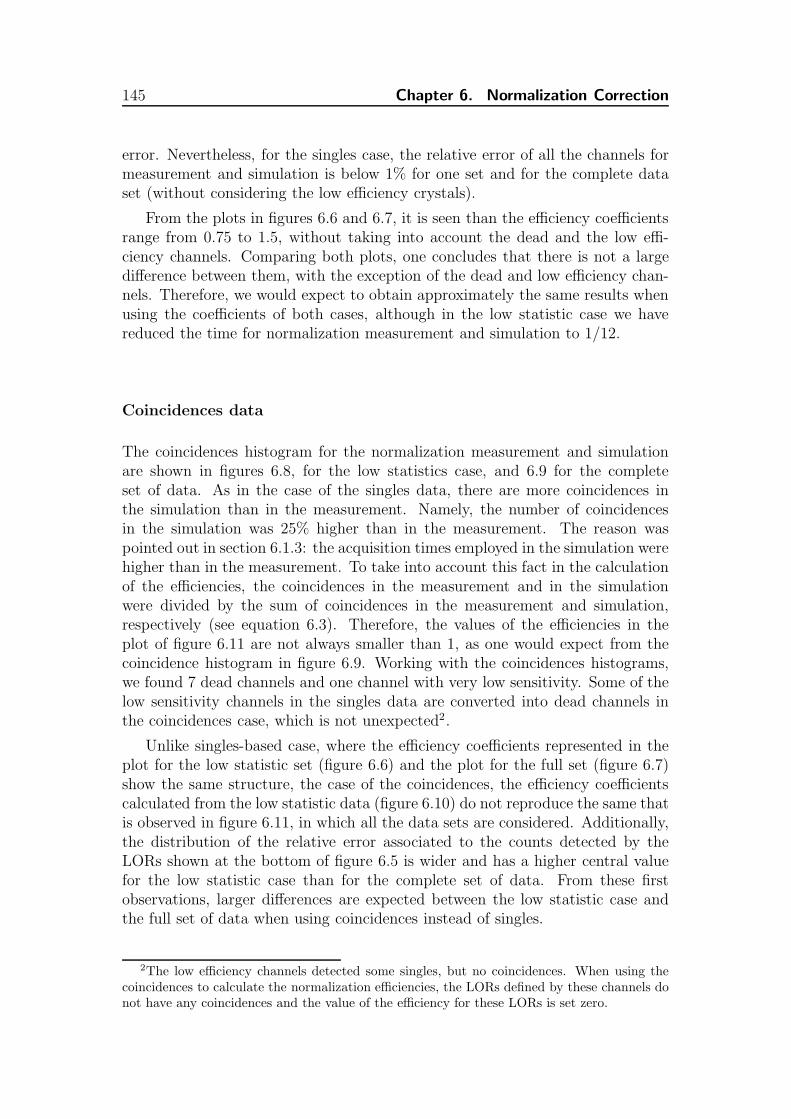
145 Chapter 6. Normalization Correction
error. Nevertheless, for the singles case, the relative error of all the channels formeasurement and simulation is below 1% for one set and for the complete dataset (without considering the low efficiency crystals).
From the plots in figures 6.6 and 6.7, it is seen than the efficiency coefficientsrange from 0.75 to 1.5, without taking into account the dead and the low effi-ciency channels. Comparing both plots, one concludes that there is not a largedifference between them, with the exception of the dead and low efficiency chan-nels. Therefore, we would expect to obtain approximately the same results whenusing the coefficients of both cases, although in the low statistic case we havereduced the time for normalization measurement and simulation to 1/12.
Coincidences data
The coincidences histogram for the normalization measurement and simulationare shown in figures 6.8, for the low statistics case, and 6.9 for the completeset of data. As in the case of the singles data, there are more coincidences inthe simulation than in the measurement. Namely, the number of coincidencesin the simulation was 25% higher than in the measurement. The reason waspointed out in section 6.1.3: the acquisition times employed in the simulation werehigher than in the measurement. To take into account this fact in the calculationof the efficiencies, the coincidences in the measurement and in the simulationwere divided by the sum of coincidences in the measurement and simulation,respectively (see equation 6.3). Therefore, the values of the efficiencies in theplot of figure 6.11 are not always smaller than 1, as one would expect from thecoincidence histogram in figure 6.9. Working with the coincidences histograms,we found 7 dead channels and one channel with very low sensitivity. Some of thelow sensitivity channels in the singles data are converted into dead channels inthe coincidences case, which is not unexpected2.
Unlike singles-based case, where the efficiency coefficients represented in theplot for the low statistic set (figure 6.6) and the plot for the full set (figure 6.7)show the same structure, the case of the coincidences, the efficiency coefficientscalculated from the low statistic data (figure 6.10) do not reproduce the same thatis observed in figure 6.11, in which all the data sets are considered. Additionally,the distribution of the relative error associated to the counts detected by theLORs shown at the bottom of figure 6.5 is wider and has a higher central valuefor the low statistic case than for the complete set of data. From these firstobservations, larger differences are expected between the low statistic case andthe full set of data when using coincidences instead of singles.
2The low efficiency channels detected some singles, but no coincidences. When using thecoincidences to calculate the normalization efficiencies, the LORs defined by these channels donot have any coincidences and the value of the efficiency for these LORs is set zero.

6.3. Results 146
6.3.2 Validity of the proposed methods
The efficiencies presented in the previous section have been used to normalizethe data from a cylindrical phantom measured in the 6-module prototype. The re-constructed images of this phantom are shown in the figure 6.12. In the transverseslices for all the images, the reconstructed shape resembles more an hexagon thana circle. This “artifact” is due to the missing angular sampling in the 6 modulessystem, when only three rotation steps of 60o are performed. The circular shapewould be recovered by increasing the number of rotation steps. Therefore, for thecomplete MADPET-II system, this artifact will not arise. Another artifact, whichis seen in the transversal slices like a circle shape, and in the coronal and sagittalslices like perpendicular lines, is present in all the cases except for the NRI-C oneand not so strong in the DN-C. The origin of this artifact could be a possiblemismatch between the simulated geometry of the scanner and the real one. Thisexplanation would be in agreement with the fact that the distortion is not seenin the case of NRI-C and it is less clear in the DN-C: In the DN-C and NRI-Cthe geometrical coefficient that would account for the mismatch is included inthe normalization factor but not in the NN case, neither in the cases of usingsingles data (DN-S and NRI-S), where the normalization takes into account onlythe intrinsic efficiencies of the crystals. The reconstructed images of the cylinderusing NRI-SLS and NRI-CLS are not presented in figure 6.12 because they showsimilar behaviours as the ones from the NRI-S and NRI-C methods, respectively.
A quantitative analysis of these images was also done by means of the relativeerror. The results are shown in the table 6.1 for all the methods after the 30th and60th iterations. The highest errors are produced by the NRI-CLS, NN, and DN-Capproaches. One would anticipate that the highest error should appear in the NNcase, because there is no correction, but is the NRI-CLS which shows the highesterror. The reason of this result is clearly the low statistic quality of the data usedto calculate the efficiencies. The result in the DN-C case is unexpected and hasnot a clear reason. One could figure out that the latter result is a combination oflower statistic quality due to the coincidences and the poor performance of directnormalization method. Without considering the NRI-CLS, the NRI methodsshow more uniform images (lower relative error) than the DN ones. As we haveobserved with the randoms correction in the chapter 4, when the correction isapplied inside of the reconstruction algorithm, the images are less noisy. In thissense, we can conclude that the normalization should be addressed within thereconstruction algorithm. When comparing the images corrected by using singlesor coincidences data, the former is preferred in terms of relative error. The NRI-Smethod, shows the lowest relative error in both iterations; also when employing1/12 of the data, the modified method (NRI-SLS) is still providing a very lowvalue for the error, even lower than in the NRI-C case. Therefore, it could bepossible to reduce the normalization measurement time when using singles tocalculate the normalization factors. On the contrary, for the coincidences-basedmethods, the time for the normalization measurement could not be shortenedand in order to achieve the same results as with the singles-based, it should be

147 Chapter 6. Normalization Correction
Table 6.1: Relative error of the voxel values inside a cylindrical ROI centeredwithin the reconstructed cylinder at the 30th and 60th iteration for the differentnormalization approaches
Method ǫrel(%) ǫrel(%)30th iteration 60th iteration
NN 17 27DN-C 17 29DN-S 16 26NRI-C 12 19
NRI-CLS 20 34NRI-S 9 14
NRI-SLS 10 15
increased.
6.4 Conclusions
Our analysis of the various singles- and coincidences-based methods does notallow us to decide which is the most appropriate to estimate the efficiencies.We nevertheless have found that normalization should be applied during thereconstruction process. This conclusion fully agrees with theory, that tells usthat all corrections should be addressed in the MLEM reconstruction algorithm,based on Poisson statistics. Although being a preliminary result, we present inthis section also the reconstructed images of a mouse heart obtained with thecomplete system. For these images, there was no normalization measurementavailable at the moment of writing this work. From the mouse measurement, itwas possible to know the dead channels. We have checked the effect of takinginto account the dead channels in the system matrix or not. In order to considerthe dead channels into the SM, the elements of the SM that are related to thedead channels, were set to zero. The reconstructed images of the mouse heart areshown in the figure 6.13. In the first row, the images were reconstructed withoutmodifying the SM. Whereas in the second row, the dead channels were accountedfor. It is obvious from the images that the corrected ones have higher quality andless artifacts. This last result supports what the theory proposes and what wefound in the 6-module system with the cylindrical phantom, i.e., the correctionsshould be performed within the reconstruction process.
Comparing the proposed methods, the reconstructed images are more uniform,but there is an artifact at the center when using the NRI-S. On the contrary, theNRI-C corrected images do not show this artifact, but they are noisier (higherrelative error). Keeping in mind that the data come from the 384-channel proto-type, there could be other reasons for the artifact that the commented mismatch,like for example misalignment in the rotation axis. Therefore, we expect thatmeasurements and simulations in the complete scanner would provide the right

6.4. Conclusions 148
answer for this open question.In terms of the acquisition time of the normalization measurement, it would
not be necessary to increase this time when using the singles data. Whereas forthe coincidence data, improvements in the uniformity of the reconstructed imagesare expected if the acquisition time would be raised.
Lastly, a few words about extracting the emitted activity from the recon-structed images. In principle, the reconstructed images should provide the emit-ted activity. But, the acquisition time of the measurement for the cylindricalsource was known very rough (by 1 minute error between sets of measurements).This leads to a big error in the determination of the emitted activity (more than20%). In addition, the reconstructed images are not corrected for attenuation.In [116], the difference between the emitted activity and the non-attenuation cor-rected reconstructed images of a 30 mm diameter mouse-like phantom is reportedto be 25%. Therefore, at this level of the study, there are too many uncertaintiesand it makes no sense to compare the approaches in their ability to recover theemitted activity.

149 Chapter 6. Normalization Correction
Crystal Number0 20 40 60 80 100 120 1400
10000
20000
30000
40000
50000
60000
70000
80000
90000
Singles Histogram - Flood Source Measurement and Simulation
Crystal Number160 180 200 220 240 260 2800
10000
20000
30000
40000
50000
60000
70000
80000
90000
Singles Histogram - Flood Source Measurement and Simulation
Crystal Number300 320 340 360 380 400 4200
10000
20000
30000
40000
50000
60000
70000
80000
90000
Singles Histogram - Flood Source Measurement and Simulation
Crystal Number440 460 480 500 520 540 5600
10000
20000
30000
40000
50000
60000
70000
80000
90000
Singles Histogram - Flood Source Measurement and Simulation
Crystal Number580 600 620 640 660 680 700 7200
10000
20000
30000
40000
50000
60000
70000
80000
90000
Singles Histogram - Flood Source Measurement and Simulation
Crystal Number720 740 760 780 800 820 840 8600
10000
20000
30000
40000
50000
60000
70000
80000
90000
Singles Histogram - Flood Source Measurement and Simulation
Crystal Number880 900 920 940 960 980 10000
10000
20000
30000
40000
50000
60000
70000
80000
90000
Singles Histogram - Flood Source Measurement and Simulation
Crystal Number1020 1040 1060 1080 1100 1120 11400
10000
20000
30000
40000
50000
60000
70000
80000
90000
Singles Histogram - Flood Source Measurement and Simulation
Figure 6.3: Singles histogram for measurement and simulation of the flood sourcein the 384-channel prototype for one set of data (low statistics case). The abcisasare the crystal number according to the numbering used in MADPET-II. Eachhistogram corresponds to one ring of crystals. Thus in each plot there are twodistinguishable parts: the front layer and back layer crystals. The rear crystalsalways detect less than the front crystals, due to the front crystals screening. Thered squares correspond to the simulations and the black line to the measurements.It can be seen that the singles histogram of the simulation presents almost thesame pattern in all the plots. But the singles histogram of the measurements doesnot due to the crystal non-uniformities. The crystal numbers with zero valuesin simulation and measurement are the crystals no present in the 384-channelprototype.

6.4. Conclusions 150
Crystal Number0 20 40 60 80 100 120 1400
200
400
600
800
1000
310×Singles Histogram - Flood Source Measurement and Simulation
Crystal Number160 180 200 220 240 260 2800
200
400
600
800
1000
310×Singles Histogram - Flood Source Measurement and Simulation
Crystal Number300 320 340 360 380 400 4200
200
400
600
800
1000
310×Singles Histogram - Flood Source Measurement and Simulation
Crystal Number440 460 480 500 520 540 5600
200
400
600
800
1000
310×Singles Histogram - Flood Source Measurement and Simulation
Crystal Number580 600 620 640 660 680 700 7200
200
400
600
800
1000
310×Singles Histogram - Flood Source Measurement and Simulation
Crystal Number720 740 760 780 800 820 840 8600
200
400
600
800
1000
310×Singles Histogram - Flood Source Measurement and Simulation
Crystal Number880 900 920 940 960 980 10000
200
400
600
800
1000
310×Singles Histogram - Flood Source Measurement and Simulation
Crystal Number1020 1040 1060 1080 1100 1120 11400
200
400
600
800
1000
310×Singles Histogram - Flood Source Measurement and Simulation
Figure 6.4: Singles histogram for measurement and simulation of the flood sourcein the 384-channel prototype for all the data sets. The abcisas are the crystalnumber according to the numbering used in MADPET-II. The red squares cor-respond to the simulations and the black line to the measurements. The crystalnumbers with zero values in simulation and measurement are the crystals nopresent in the 384-channel prototype.
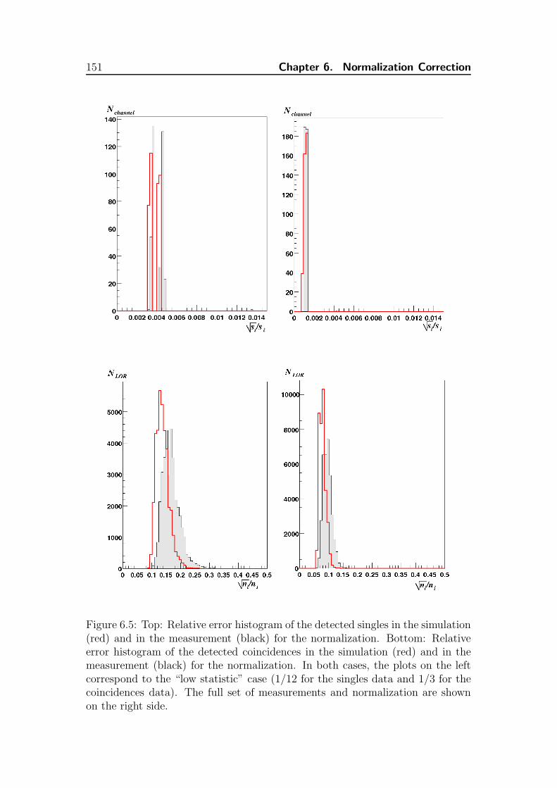
151 Chapter 6. Normalization Correction
Figure 6.5: Top: Relative error histogram of the detected singles in the simulation(red) and in the measurement (black) for the normalization. Bottom: Relativeerror histogram of the detected coincidences in the simulation (red) and in themeasurement (black) for the normalization. In both cases, the plots on the leftcorrespond to the “low statistic” case (1/12 for the singles data and 1/3 for thecoincidences data). The full set of measurements and normalization are shownon the right side.

6.4. Conclusions 152
0
0.5
1
1.5
2
2.5
Crystal Number (modules 17,0,1)0 20 40 60 80 100 120 140 160 180
Cry
stal
Num
ber
(mod
ules
8,9
,10)
0
20
40
60
80
100
120
140
160
180
Efficiency coeficients (Singles Low Statistics)Efficiency coeficients (Singles Low Statistics)
Figure 6.6: Efficiency coefficients for each LOR that belongs to the 384-channelprototype calculated from one set of the singles data. The crystal numbers donot correspond to the numbering used in MADPET-II, the numbering plottedwas used in order to represent all the LORs in the graph in a compact way. Inthe abcisas, the first 64 crystals belong to module 17, the next 64 to module 0,and the last 64 to module 1. In each module the first 32 channels represent thecrystals in the front layer, and the last 32 to the back layer. The same structureis followed in the ordinates, but the modules are different, the ones in front ofthe 17, 0 and 1. In this way, the first 64 crystal numbers are for the module 8,the next 64 for the module 9 and the last 64 for the module 10.

153 Chapter 6. Normalization Correction
0
0.5
1
1.5
2
2.5
Crystal Number (modules 17,0,1)0 20 40 60 80 100 120 140 160 180
Cry
stal
Num
ber
(mod
ules
8,9
,10)
0
20
40
60
80
100
120
140
160
180
Efficiency coeficients (Singles)Efficiency coeficients (Singles)
Figure 6.7: Efficiency coefficients for each LOR that belongs to the 384-channelprototype calculated from all the singles data. The numbering used in this his-togram is explained in the caption of figure 6.6.

6.4. Conclusions 154
0
20
40
60
80
100
120
Crystal Number (modules 17,0,1)0 20 40 60 80 100 120 140 160 180
Cry
stal
Num
ber
(mod
ules
8,9
,10)
0
20
40
60
80
100
120
140
160
180
Measurement Flood SourceMeasurement Flood Source
0
20
40
60
80
100
120
Crystal Number (modules 17,0,1)0 20 40 60 80 100 120 140 160 180
Cry
stal
Num
ber
(mod
ules
8,9
,10)
0
20
40
60
80
100
120
140
160
180
Simulation Flood SourceSimulation Flood Source
Figure 6.8: Low Statistics Coincidences histogram for measurement and simula-tion of the flood source in the 384-channel prototype. The numbering used inthis histogram is explained in the caption of figure 6.6.
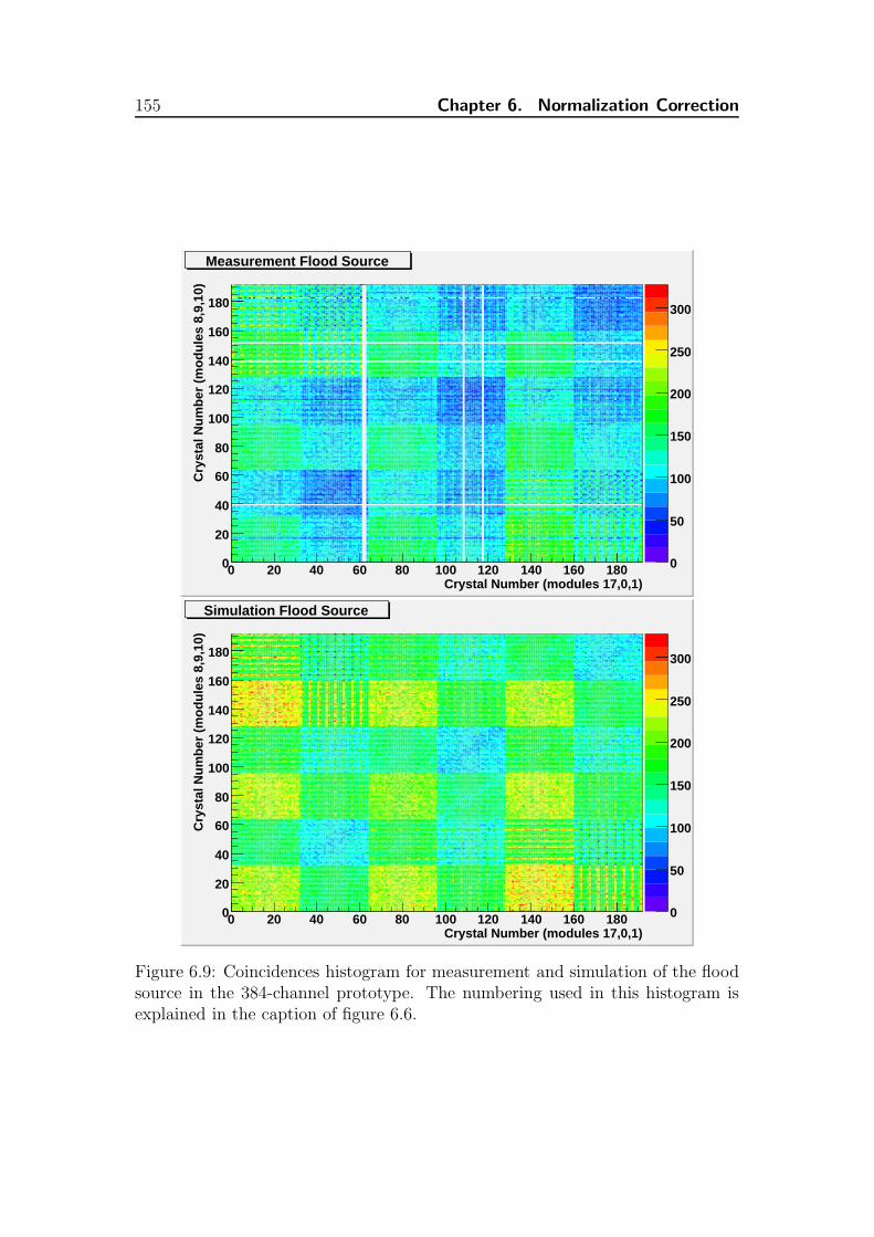
155 Chapter 6. Normalization Correction
0
50
100
150
200
250
300
Crystal Number (modules 17,0,1)0 20 40 60 80 100 120 140 160 180
Cry
stal
Num
ber
(mod
ules
8,9
,10)
0
20
40
60
80
100
120
140
160
180
Measurement Flood SourceMeasurement Flood Source
0
50
100
150
200
250
300
Crystal Number (modules 17,0,1)0 20 40 60 80 100 120 140 160 180
Cry
stal
Num
ber
(mod
ules
8,9
,10)
0
20
40
60
80
100
120
140
160
180
Simulation Flood SourceSimulation Flood Source
Figure 6.9: Coincidences histogram for measurement and simulation of the floodsource in the 384-channel prototype. The numbering used in this histogram isexplained in the caption of figure 6.6.
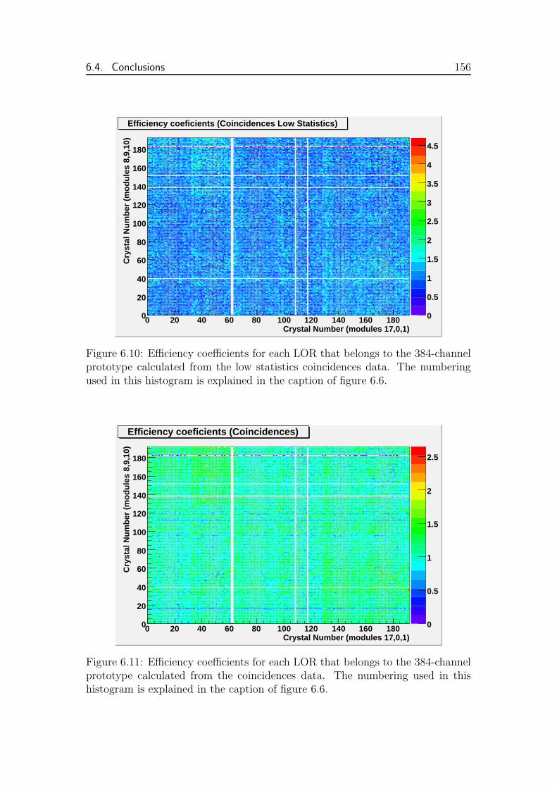
6.4. Conclusions 156
0
0.5
1
1.5
2
2.5
3
3.5
4
4.5
Crystal Number (modules 17,0,1)0 20 40 60 80 100 120 140 160 180
Cry
stal
Num
ber
(mod
ules
8,9
,10)
0
20
40
60
80
100
120
140
160
180
Efficiency coeficients (Coincidences Low Statistics)Efficiency coeficients (Coincidences Low Statistics)
Figure 6.10: Efficiency coefficients for each LOR that belongs to the 384-channelprototype calculated from the low statistics coincidences data. The numberingused in this histogram is explained in the caption of figure 6.6.
0
0.5
1
1.5
2
2.5
Crystal Number (modules 17,0,1)0 20 40 60 80 100 120 140 160 180
Cry
stal
Num
ber
(mod
ules
8,9
,10)
0
20
40
60
80
100
120
140
160
180
Efficiency coeficients (Coincidences)Efficiency coeficients (Coincidences)
Figure 6.11: Efficiency coefficients for each LOR that belongs to the 384-channelprototype calculated from the coincidences data. The numbering used in thishistogram is explained in the caption of figure 6.6.
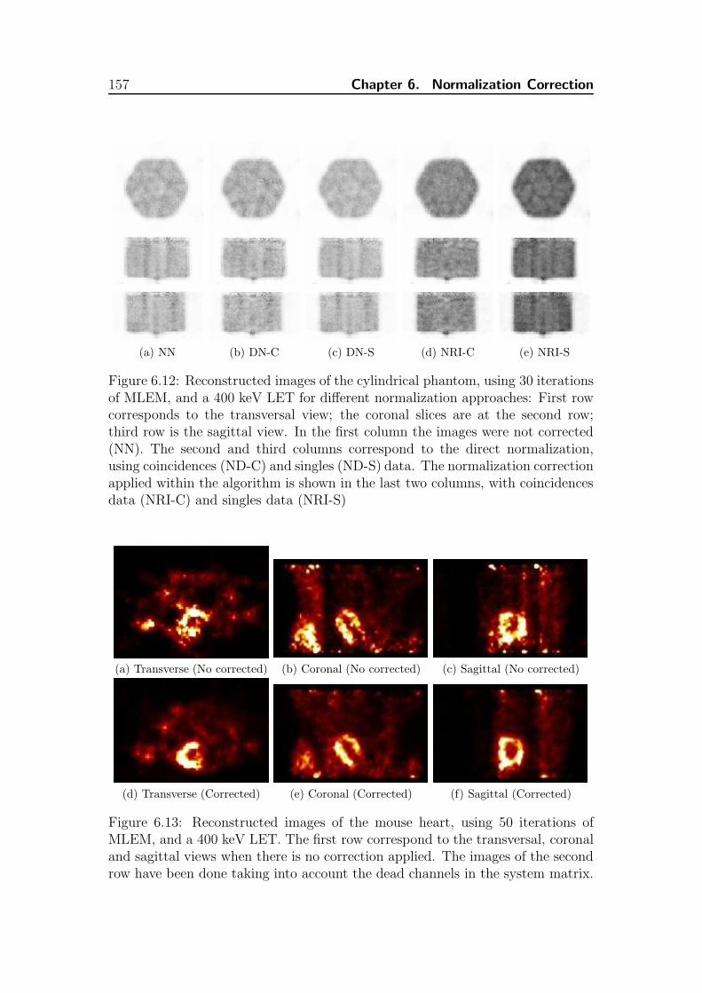
157 Chapter 6. Normalization Correction
(a) NN (b) DN-C (c) DN-S (d) NRI-C (e) NRI-S
Figure 6.12: Reconstructed images of the cylindrical phantom, using 30 iterationsof MLEM, and a 400 keV LET for different normalization approaches: First rowcorresponds to the transversal view; the coronal slices are at the second row;third row is the sagittal view. In the first column the images were not corrected(NN). The second and third columns correspond to the direct normalization,using coincidences (ND-C) and singles (ND-S) data. The normalization correctionapplied within the algorithm is shown in the last two columns, with coincidencesdata (NRI-C) and singles data (NRI-S)
(a) Transverse (No corrected) (b) Coronal (No corrected) (c) Sagittal (No corrected)
(d) Transverse (Corrected) (e) Coronal (Corrected) (f) Sagittal (Corrected)
Figure 6.13: Reconstructed images of the mouse heart, using 50 iterations ofMLEM, and a 400 keV LET. The first row correspond to the transversal, coronaland sagittal views when there is no correction applied. The images of the secondrow have been done taking into account the dead channels in the system matrix.

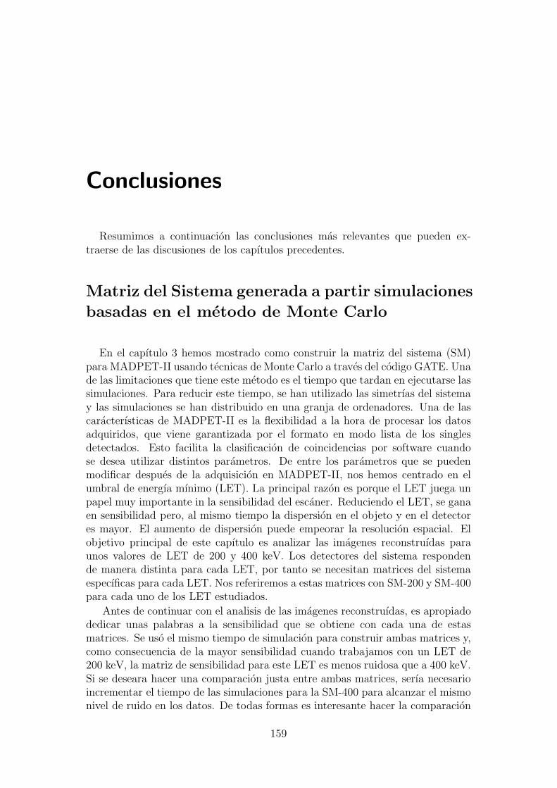
Conclusiones
Resumimos a continuacion las conclusiones mas relevantes que pueden ex-traerse de las discusiones de los capıtulos precedentes.
Matriz del Sistema generada a partir simulaciones
basadas en el metodo de Monte Carlo
En el capıtulo 3 hemos mostrado como construir la matriz del sistema (SM)para MADPET-II usando tecnicas de Monte Carlo a traves del codigo GATE. Unade las limitaciones que tiene este metodo es el tiempo que tardan en ejecutarse lassimulaciones. Para reducir este tiempo, se han utilizado las simetrıas del sistemay las simulaciones se han distribuido en una granja de ordenadores. Una de lascaracterısticas de MADPET-II es la flexibilidad a la hora de procesar los datosadquiridos, que viene garantizada por el formato en modo lista de los singlesdetectados. Esto facilita la clasificacion de coincidencias por software cuandose desea utilizar distintos parametros. De entre los parametros que se puedenmodificar despues de la adquisicion en MADPET-II, nos hemos centrado en elumbral de energıa mınimo (LET). La principal razon es porque el LET juega unpapel muy importante in la sensibilidad del escaner. Reduciendo el LET, se ganaen sensibilidad pero, al mismo tiempo la dispersion en el objeto y en el detectores mayor. El aumento de dispersion puede empeorar la resolucion espacial. Elobjetivo principal de este capıtulo es analizar las imagenes reconstruıdas paraunos valores de LET de 200 y 400 keV. Los detectores del sistema respondende manera distinta para cada LET, por tanto se necesitan matrices del sistemaespecıficas para cada LET. Nos referiremos a estas matrices con SM-200 y SM-400para cada uno de los LET estudiados.
Antes de continuar con el analisis de las imagenes reconstruıdas, es apropiadodedicar unas palabras a la sensibilidad que se obtiene con cada una de estasmatrices. Se uso el mismo tiempo de simulacion para construir ambas matrices y,como consecuencia de la mayor sensibilidad cuando trabajamos con un LET de200 keV, la matriz de sensibilidad para este LET es menos ruidosa que a 400 keV.Si se deseara hacer una comparacion justa entre ambas matrices, serıa necesarioincrementar el tiempo de las simulaciones para la SM-400 para alcanzar el mismonivel de ruido en los datos. De todas formas es interesante hacer la comparacion
159
160
para contrastar el comportamiento de ambas matrices cuando se ha empleado elmismo tiempo en generarlas.
En el analisis de las imagenes reconstruıdas, en cuanto a la resolucion espacialno se han observado diferencias en las imagenes reconstruıdas del maniquıDerenzoy, en ambos casos, las capilares mas pequenas que se pueden distinguir son lasde diametro 1.5 mm. Las diferencias entre ambas matrices aparecen cuando secalcula la FWHM de las fuentes puntuales que se encuentran cerca del lımite delcampo de vision. De este resultado se puede concluir que la dispersion en losdetectores presente en el caso de SM-200 afecta mas a la resolucion espacial queel ruido estadıstico, que es mayor en el caso de SM-400.
Por otro lado, la matriz SM-200 produce mejores resultados en terminos decuantificacion de la actividad y deteccion de lesion, como se observa del analisisde las correspondientes figuras de merito (FOM). Claramente, el ruido estadısticomas alto tanto en la SM y como en el histograma de LORes a la energıa umbralde 400 keV es el factor que produce este resultado. La conclusion de esta parte esque una sensibilidad mayor, que implica menor ruido estadıstico para el mismotiempo de adquisicion, es muy importante para cuantificar la distribucion deactividad y para mejorar la deteccion de lesiones.
El ruido estadıstico en el histograma de LORes se puede reducir aumentandoel tiempo de adquisicion en la medida a un LET de 400 keV. Esto no fue estudiado,pero es importante el tener en cuenta que hay medidas que estan ligadas a tiemposde adquisicion cortos, como estudios dinamicos para modelado farmacocinetico.Ademas es muy importante conocer la concentracion de trazador en estos estudiosy, como hemos visto, bajos LET ofrecen informacion mas precisa de la distribucionde actividad. Por otro lado, en el caso de estudios estaticos, donde no estamoslimitados a tiempos reducidos, trabajar con LETs de 400 keV proporcionarıamejores imagenes en cuanto a visualizacion de pequenos detalles. Para obtener losmismos resultados a nivel de cuantificacion en el caso de SM-400, en comparacioncon el de SM-200, se necesitarıa simular por mas tiempo para obtener una matrizdel sistema menos ruidosa.
De los resultados mostrados en este capıtulo, se puede concluir que la flexibil-idad que ofrece la adquisicion en modo lista de sucesos singles del MADPET-IIes una caracterıstica muy util, porque permite adaptar el LET al tipo de estudioque se desea realizar y obtener los mejores resultados para esa tarea especıfica.
Correccion por coincidencias accidentales
Los metodos de la ventana restrasada (DW) y de la tasa de singles (SR) sehan usado para estimar las coincidencias accidentales o random para varios val-ores de la energıa umbral mınima. Para LETs menores de 255 keV, se observauna notable sobreestimacion de las coincidencias random, siendo mayor para elmetodo de SR que de DW. La sobreestimacion encontrada en los metodos DWy su modificado DW’ no se puede explicar a partir del retraso elegido para la

161
ventana temporal. El responable de esta sobreestimacion es la dispersion que seda entre los cristales detectores, que es muy importante a bajas energıas umbralesmınimas. Estos resultados se presentaron para una actividad total de 3.7 MBq.Si aumentamos la actividad, la sobreestimacion aumenta para el metodo de SR,mientras que permanece constante para el metodo de DW. Este comportamientodel metodo SR es debido al incremento del numero de coincidencias randomtriples para estas actividades. Las imagenes que se obtienen cuando la correccionpor coincidencias random se aplica en el algoritmo de reconstruccion son mejoresen terminos del cociente senal-ruido, niveles de ruido y proporcionando valores deactividad absoluta (con alguna excepcion en la que en ambos casos se comportande la misma manera) que las imagenes reconstuıdas con datos precorregidos. Soloen el caso de ME (figura de merito que mide sucesos que no han sido situadosde manera correcta en la imagen reconstruıda), las imagenes precorregidas mues-tran mejor resultados. En general, para todos los LETs estudiados, el metodoDW es mas exacto para la obtencion de la actividad absoluta de las imagenes re-construıdas, debido a la menor sobreestimacion de coincidencias random, aunquela diferencia con SR a 400 keV no es muy importante para las actividades es-tudiadas mas bajas. Las discrepancias observadas para las imagenes corregidascorrespondientes a la actividad mas baja (2%-4% en el peor caso) no suponenuna cuestion importante, si consideramos que la exactitud de las concentracionesde actividad para imagenes no corregidas por atenuacion es de -26.4% para unfantoma representativo de un raton y -38.5% para un fantoma que representa unarata [116]. Sin embargo, la dependencia de la sobreestimacion con la actividad dela fuente nos muestra que estas discrepancias son mayores para actividades masaltas. A LET de 200 keV, las imagenes reconstruıdas no presentan una diferenciasustancial en terminos de ruido para la actividad mas baja. Cuando la actividadde la fuente aumenta, la sobreestimacion produce un aumento de ruido para lasimagenes corregidas con el metodo SR a LET de 200 keV. A LET de 400 keV,las imagenes reconstruıdas usando SR muestran un menor ruido para todas lasactividades estudiadas. La pregunta sobre cual es el LET mas apropiado todavıaqueda sin contestar. Con LETs por debajo de 255 keV, hay una subestimacionde la actividad reconstruıda, pero las imagenes son menos ruidosas debido a lamayor sensibilidad. Trabajando a estos LETs, el metodo DW es el preferido.El ruido de las imagenes podrıa ser reducido usando tecnicas de reduccion dela varianza para las coincidencias aleatorias discutidas en [102]. Para LETs porencima de 255 keV, la cuantificacion no supone un problema, la sensibilidad delsistema es menor y las imagenes son mas ruidosas, por tanto el metodo SR es elmas apropiado porque es el que muestra menor ruido. Para el caso de actividadesmas altas y para el metodo de SR, la sobrestimacion tiene un efecto mayor y, portanto, debe ser corregida. Por tanto, como trabajo futuro se deberıa estudiarcomo se puede corregir la sobrestimacion en el numero de coincidencias randomusando los metodos de DW y SR para actividades altas. Aunque este estudio seha llevado a cabo con la geometrıa de MADPET-II, se espera que los resultadossean validos para otros sistemas formados por cristales finamente granulados.

162
Coincidencias triples
Las coincidencias tripes y su impacto en los metodos de estimacion de co-incidencias random se han estudiado en este capıtulo. El principal beneficio deconsiderar este tipo de sucesos para la reconstruccion es que incrementa la sensi-bilidad del sistema. Ademas, en el anterior capıtulo se encontro que las coinciden-cias triples podrıan ser de ayuda para resolver el problema de la sobrestimacionde coincidencias accidentales. Cuando se introducen las triples coincidencias, esnecesario conocer como procesarlas para no deteriorar la calidad de las imagenesreconstruıdas.
Primeramente se confirmo que la sensibilidad aumenta un 20% para un LETde 200 keV cuando se tienen en cuenta las coincidencias triples. Posteriormente,antes de empezar con la correccion por coincidencias random, era importanteverificar que no se producıa una degradacion de las imagenes reconstruıdas cuandose utilizaban coincidencias verdaderas tanto dobles como triples. Para hacer esto,se compararon las imagenes obtenidas usando una matriz del sistema que solocontiene dobles coincidencias y las que se produjeron con una matriz del sistemaque considera dobles y triples coincidencias. Para el analisis de la resolucionespacial, se simulo un fantoma de Derenzo y unos capilares paralelos al eje delescaner y distribuıdos horizontanmente, de manera que cubren el campo de visiondel sistema. En el caso de las imagenes de Derenzo, no solo no encontramos ninguntipo de degradacion visula de la imagen, sino que ademas se pueden identificaralgunas de las varillas de 1.2 mm de diametro que se encuentran cerca del centrodel campo de vision en el caso de la matriz del sistema que tiene dobles y triplescoincidencias. En el caso de los capilares horizontales, pequenas diferencias seobservan en la FWTM para las fuentes situdadas cerca del lımite del campode vision. Para examinar las capacidades para recuperar la actividad emitidase ha usado el fantoma hot-cold-background. Es posible recuperar la actividademitida en las imagenes reconstruıdas de este fantoma con ambas matrices. Portanto, a partir de estos primeros resultados obtenidos usando solo coincidenciasverdaderas (dobles y triples), podemos concluir que no existe deterioro de lasimagenes reconstruıdas usando dobles y tripes coincidencias. Ademas de queen terminos de la resolucion espacial, las imagenes donde se incluyen los triplesmuestran mayor calidad.
En cuanto a la correccion por coincidencias random, el considerar los sucesostriples nos lleva a tener que modificar la forma de estimar estas coincidenciaspara incluir estos sucesos. Hemos adaptado los metodos de DW y SR y hemosencontrado que al incluir las triples coincidencias, la sobrestimacion de randoms(mostrada en en capıtulo anterior) queda reducida notablemente. Ademas, lasimagenes reconstruıdas, corregidas por coincidencias random y con coinciden-cias triples, no muestran ningun artefacto consecuencia de la modificacion de losmetodos de estimacion de coincidencias accidentales y que supusiera el no poderutilizar los metodos modificados. Al contrario, no existe ninguna apreciable difer-encia visual entre ellas y las imagenes obtenidas usando solo doble coincidencias.

163
Del analisis cuantitativo se obtiene que la introduccion de las triples coincidenciasresuelve la subestimacion de la actividad y, al ser la sensibilidad mayor, el ruidode las imagenes es menor.
Por tanto, las coincidencias triples se presentan como buenas candidatas paraser incluıdas en el proceso de reconstruccion porque, por un lado, aumentan lasensibilidad del sistema y por el otro reducen la sobrestimacion de coincidenciasrandom para bajos LET. Aunque no hay que olvidar que los resultados presenta-dos aquıson para una matriz del sistema hecha para un solo corte del FOV. Portanto, serıa necesario confirmar estos resultados en una matriz del sistema en 3Dy para objetos mayores.
Finalmente, en este trabajo nos hemos centrado en un unico algoritmo paraclasificar las coincidencias que usa una unica ventana temporal de coincidencias.Existen otro tipo de algoritmos que utilizan multiples ventanas de coincidenciasy cambian la clasificacion de lo que es una doble y triple coincidencia. Para unmayor analisis sobre esta cuestion referimos al trabajo [129], donde se hace unacomparacion entre metodos de clasificacion que usan ventana temporal unica ylos que utilizan multiples ventanas.
Normalizacion
Para resumir los resultados cuantitativos y cualitativos de esta parte, no esevidente cual es el mejor metodo para estimar las eficiencias entre los metodosbasados en singles y en dobles, pero lo que sıqueda confirmado es que la nor-malizacion se debe de aplicar durante el proceso de reconstruccion. Esta ultimaconclusion esta de acuerdo con la teorıa, que propone que todas las correccionesse deben de considerar durante el algoritmo de reconstruccion MLEM, basado enel modelo estadıstico de Poisson. Aunque es un resultado preliminar, presenta-mos en esta seccion las imagenes reconstruıdas del corazon de un raton que fuemedido con el sistema completo. Para el sistema completo no hay medidas pararealizar la normalizacion. Pero, de las medidas tomadas al corazon del raton, fueposible conocer los canales muertos del sistema y hemos comprobado el efecto detener en cuenta los canales muertos en la matriz del sistema o no tenerlos. Paracontar con los canales muertos en la SM, los elementos de esta que estan for-mados por un canal muerto se hacen iguales a cero. Las imagenes reconstruıdasdel corazon del raton se muestran en la figura 6.13. En la primera lınea, lasimagenes fueron reconstruıdas sin modificar la matriz del sistema. Mientras queen la lınea de abajo, los canales muertos se tuvieron en cuenta. Es obvio a partirde las imagenes, que las corregidas tienen una mayor calidad y presentan menosartefactos. Este ultimo resultado apoya lo que la teorıa propone y lo que hemosencontrado en el sistema de 6 modulos con la fuente cilındrica: las correccionesse deben de llevar a cabo dentro del proceso de reconstruccion.
Comparando los metodos propuestos, las imagenes reconstruıdas son mas uni-formes con el NRI-S, pero hay un artefacto en el centro de la imagen. Por el con-

164
trario, las imagenes corregidas usando NRI-C no muestran este artefacto, peroson mas ruidosas (error relativo mas grande). Como los datos vienen del sistemade 384 canales, podrıa existir otra razon para el artefacto que el comentado de-sajuste, como por ejemplo que el eje de rotacion no estuviera bien alineado. Portanto, esperamos que medidas y simulaciones del sistema completo nos propor-cionen la respuesta a esta pregunta que queda abierta.
En terminos del tiempo de adquisicion de la medida de normalizacion, encaso de usar los singles, no serıa necesario aumentarlo. Mientras que cuandose usan las coincidencias, se esperan mejoras en la uniformidad de las imagenesreconstruıdas si se incrementara el tiempo de adquisicion.
Finalmente, unas palabras relacionadas con la obtencion de la actividad emi-tida a partir de las imagenes reconstruıdas. En principio, las imagenes recon-struıdas deberıan proporcionar la actividad emitida. Pero el tiempo de adquisicionde la medida de la fuente cilındrica era conocido de manera muy imprecisa (1 min-uto de error entre sets de medidas). Esto lleva a un gran error en el calculo dela actividad emitida (mayor de un 20%). Ademas, las imagenes reconstruıdas nose corrigieron por atenuacion. En [116], la diferencia entre la actividad emitida yla actividad obtenida en las imagenes reconstruıdas de un fantoma tamano ratonde 30 mm de diametro es 25%. Por tanto, al nivel que estamos en este estu-dio, hay demasiadas indeterminaciones y no tiene sentido comparar las diferentespropuestas en su capacidad para recuperar la actividad emitida.

List of Abbreviations
• ADC: Analog to Digital Converter
• APD: Avalanche PhotoDiode
• ASIC: Application Specific Integrated Circuit
• CRC: Contrast Recovery Coefficient
• CSP: Charge Sensitive Preamplifier
• CT: Computer Tomography
• D: Discrepancy
• DN: Direct Normalization
• DN-C: Direct Normalization Coincidences-based
• DN-S: Direct Normalization Singles-based
• DOI: Depth Of Interaction
• DW: Delayed Window
• DWSub: Delayed Window Subtracted (prior reconstruction)
• DWmd: Delayed Window maximum distance
• DWme: Delayed Window maximum energy
• EM: Expectation Maximization
• FBP: Filtered Back Projection
• FOM: Figure Of Merit
• FOV: Field Of View
• FPGA: Field Programmable Gate Array
• FWHM: Full Width Half Maximum
165

166
• FWTM: Full Width Tenth Maximum
• GATE: Geant4 Application for Tomographic Emission
• HCB: Hot-Cold-Background
• IC: Inter-Crystal
• ICS: Inter-Crystal Scatter
• IF: Identification Fraction
• LCG: LHC Computing Grid
• LET: Low Energy Threshold
• LHC: Large Hadron Collider
• LOR: Line Of Response
• MADPET: Munich Avalanche photoDiode Positrom Emission Tomograph
• MC: Monte Carlo
• MCSM: Monte Carlo System Matrix
• MD: Maximum Distance
• ME: Maximum Energy
• ME: Mispositioned Events
• ML: Maximum Likelihood
• MLEM: Maximum Likelihood Expectation Maximization
• NEMA: National Electrical Manufacturers Association
• NF : Normalization Factor
• NN: No Normalization
• NRI: Normalization within the Reconstruction of the Image
• NRI-C: Normalization within the Reconstruction of the Image, Coincidences-based
• NRI-CLS: Normalization within the Reconstruction of the Image, Coincidences-based with Low Statistics data
• NRI-S: Normalization within the Reconstruction of the Image, Singles-based

167
• NRI-SLS: Normalization within the Reconstruction of the Image, Singles-based with Low Statistics Data
• OSEM: Ordered Subsets Expectattion Maximization
• PET: Positron Emission Tomography
• PMT: PhotoMultiplier Tube
• PSF: Point Spread Function
• ROI: Region Of Interest
• SiPM Silicon PhotoMultiplier
• SM: System Matrix
• SNR: Signal-to-Noise Ratio
• SPECT: Single Photon Emission Computed Tomography
• SR: Singles Rate
• SRSub: Singles Rate Subtracted (prior reconstruction)
• SRns: Singles Rate new sorting
• STIR: Software for Tomographic Image Reconstruction
• TDC: Time to Digital Converter
• TH: Time Histogram
• VO: Virtual Organization
• VOR: Volume Of Response
• 1D: 1 Dimensional
• 2D: 2 Dimensional
• 3D: 3 Dimensional


Bibliography
[1] Phelps M E, Hoffman E J, Mullani N A, Ter-Pogossian M M. 1975 Ap-plication of annihilation coincidence detection to transaxial reconstructiontomography. J. Nuc. Med. 16 210-224
[2] Harper M D. 2004 Positronium: review of simmetry, conserved quantitiesand decay for the radiological physicist. Med. Phys. 31 57-61
[3] Hoffman E J, Huang S-C, Phelps M E, Kuhl D E. 1981 Quantitation inpositron emission computed tomography. IV. Effect of accidental coinci-dences. J. Comput. Assist. Tomogr. 5 391-400
[4] Strother S C, Casey M E, Hoffman E J. 1990 Measuring PET scannersensitivity: relating count rates to image signal-to-noise ratios using noiseequivalent counts. IEEE Trans. Nucl. Sci. 37 783-788
[5] Hoffman E J, Phelps M E. 1976 An analysis of some of the physical aspectsof positron transaxial tomography. Comput. Biol. Med. 6 345-360
[6] Moses W W, Derenzo S E. 1993 Empirical observation of resolution degra-dation in positron emission tomographs utilizing block detectors. J. Nucl.Med. 34 101P
[7] Budinger T F, Derenzo S E, Huesman R H, Jagust W J, Valk P E. 1991High resolution positron emission tomography for medical science studies.Acta. Radiol. 376 15-23
[8] Fowler J S, Wolf A P. 1986 Positron emitter labeled compounds: Prioritiesand problems. In “Positron Emission Tomography and Autorradiography”(M. Phelps, J. Mazziotta, H. Schelbert, eds.), pp 391-450. Raven Press,New York
[9] Phelps ME. 2000 PET: The merging of Biology and Imaging into MolecularImaging. J. Nucl. Med. 41 558-564
[10] Bailey D L, Jones T, Spinks T J. 1991 A method of measuring the absolutsensitivity of positron emission tomographic scanners. Eur. J. Nucl. Med.18 374-379
169

Bibliography 170
[11] Chatziioannou A F, Cherry S R, Shao Y, Silverman R W, Meadors K,Farquhar T H, Pedarsani M, Phelps M E. 1999 Performance evaluation ofmicroPET: A high-resolution lutetium oxy-orthosilicate PET scanner foranimal imaging. J. Nucl. Med. 40 1164-1175
[12] Marler J, McCauley T, Reucroft S, Swain J, Budil D, Kolaczkowski S. 2000Studies of avalanche photodiode performance in a high magnetic field. Nucl.Instrum. Methods A 449 311-313
[13] Buzhan P, Dolgoshein B, Filatov L, Ilyin A, Kantzerov V, et al. 2003 Siliconphotomultiplier and its possible applications. Nucl. Instrum. Methods A504 48-52
[14] Georgievskya E A, Klemin S N, Filatov L A, Buzhan P J, Dolgoshein BA et al. 2003 The solid state silicon photomultiplier for a wide range ofapplications. Proc. SPIE Int. Soc. Opt. Eng. (USA) 5126 3742
[15] Golovin V, Saveliev V. 2004 Novel type of avalanche photodetector withGeiger mode operation. Nucl. Instrum. Methods A 518 560-564
[16] Hume S P, Gunn R N, Jones T. 1998 Pharmacological constraints associatedwith positron emission tomographic scanning of small laboratory animals.Eur. J. Nucl. Med. 25 173-176
[17] Shepp L A, Vardi Y. 1982 Maximum likelihood estimation for emissiontomography. IEEE Trans Med. Imaging 1 113-121
[18] Hudson H M, Larkin R S. 1994 Accelerated image reconstruction usingordered subsets of projection data. IEEE Trans Med. Imaging 13 601-609
[19] Wernick M N and Aarsvold J N. 2004 Emission Tomography, The Funda-mentals of PET and SPECT (Elsevier Academic Press)
[20] Natterer F and Wubbeling F. 2001 Mathematical Methods in Image Recon-struction (SIAM, Philadelphia)
[21] Natterer F. 1986 The mathematics of computerized tomography (Wiley, NewYork)
[22] Townsend D W and Defrise M 1993 Image Reconstruction methods inpositron tomography (Academic Training Lectures, CERN)
[23] Colsher J G. 1980 Fully three-dimensional Positron Emission TomographyPhys. Med. Biol. 25 103-115
[24] Chu G and Tam K C. 1977 3D imaging in the positron camera using Fouriertechniques Phys. Med. Biol. 22 245-265
[25] Rogers J G, Harrop R, Kinahan P E. 1987 The theory of three-dimensionalimage reconstruction IEEE Trans. Med. Imaging 6 239-243
171 Bibliography
[26] Kinahan P E, Rogers J G, Harrop R and Johnson R. 1988 Three-dimensional image reconstruction in object space IEEE Trans. Nucl. Sci.35 635-638
[27] Kinahan P E and Rogers J G. 1989 Analytic 3D Image Reconstructionusing all detected events IEEE Trans. Nucl. Sci. 36 964-968
[28] Qi J, Leahy R M, Hsu C, Farquhar T H and Cherry S R. 1996 Fully 3DBayesian image reconstruction for the ECAT EXACT HR+’ IEEE Trans.Nuc. Sci. 45 1096-1103
[29] Yavus M and Fessler J A. 1996 Objective functions for tomographic re-construction from randoms-precorrected PET scans IEEE NSS MIC Conf.Rec. 2 1067-1071
[30] Leahy R M and Qi J. 2000 Statistical approaches in quantitative positronemission tomography Statistics and Computing 10 147-165
[31] Compton A H. 1923 A quantum theory of the scattering of X-rays by lightelements Phys. Rev. 21 483-502
[32] Electron Gamma Shower (EGS) Monte Carlo Radiation Transport Code.http://pager.lbl.gov/egs/egs.html
[33] MCNP directory. http://www-xdiv.lanl.gov/XCI/PROJECTS/MCNP/
[34] Halbleib JA, Kensek RP, Mehlhorn TA, Valdez GD, Seltzer SM, Berger MJ.ITS Version 3.0: the integrated TIGER series of coupled electron/photonMonte Carlo transport codes. Sandia National Laboratories. Technical Re-port SAND91-1634, 1992
[35] GEANT 3 home page. http://wwwasd.web.cern.ch/wwwasd/geant/
[36] GEANT 4 home page. http://geant4.web.cern.ch/geant4/
[37] Ljungberg M, Strand SE. 1989 A Monte Carlo program for the simulationof scintillation camera characteristics Comput. Methods Prog. Biomed. 29257-272
[38] Yanch J C, Dobrzeniecki A B, Ramanathan C, Behrman R. 1992 Physicallyrealistic Monte Carlo simulation of source, collimator and tomographic dataacquisition Phys. Med. Biol. 37 853-870
[39] Yanch J C, Dobrzeniecki A B. 1993 Monte Carlo simulation in SPECT:complete 3D modelling of source, collimator and tomographic data acqui-sition IEEE Trans. Nucl. Sci. 40 198-203
[40] Smith M F. 1993 Modelling photon transport in non-uniform media forSPECT with a vectorized Monte Carlo code Phys. Med. Biol. 38 1459-1474

Bibliography 172
[41] Smith M F, Floyd C D, Jaszczak R J. 1993 A vectorized Monte Carlo codefor modelling photon transport in SPECT Med. Phys. 20 1121-1127
[42] Thompson C J, Cantu J M, Picard Y. 1992 PETSIM: Monte Carlo programsimulation of all sensitivity and resolution parameters of cilindrical positronimaging systems. Phys. Med. Biol. 37 731-749
[43] Thompson C J, Picard Y. 1998 PETSIM: Monte Carlo simulation ofpositron imaging systems. In: Ljungberg M, Strand SE, King M, editors.Monte Carlo calculations in nuclear medicine. Bristol and Philadelphia:IOP Publishing, 233-248
[44] Zaidi H, Labbe C, Morel C. 1998 EIDOLON: Implementation of an envi-ronment for Monte Carlo simulation of fully 3D positron tomography on ahigh performance parallel platform Parallel Comput. 24 523-536
[45] Reilhac A, Gregoire M C, Costes N, Lavenne F, Pierre C, Diou A et al. 1999A PET Monte Carlo simulator from numerical phantoms: validation againstthe EXACT ECAT HR+ scanner. IEEE NSS MIC Conf. Rec. 1527-1536
[46] Castiglioni I, Cremonesi O, Gilardi M C, Bettinardi V, Rizzo G, Savi A etal. 1999 Scatter correction techniques in 3D PET: a Monte Carlo evaluation.IEEE Tans. Nucl. Sci. 46 2053-2058
[47] Harrison R L, Vannoy S D, Haynor D R, Gillipsie S B, Kaplan M S, LewellenT K. 1993 Preliminary experience with the photon history generator moduleof a public domain simulation system for emission tomography. IEEE NSSMIC Conf. Rec. 1154-1158
[48] SIMSET home page. http://depts.washington.edu/simset/html/simset main.html
[49] GATE home page. http://opengatecollaboration.healthgrid.org/
[50] Jan S, Santin G, Strul D, Staelens S, Assie K, Autret D, Avner S, BarbierR, Bardies M, Bloomfield P M, Brasse D, Breton V, Bruyndonckx P, BuvatI, Chatziioannou A F, Choi Y, Chung Y H, Comtat C, Donnarieix D, FerrerL, Glick S J, Groiselle C J, Guez D, Honore P F, Kerhoas-Cavata S, KirovA S, Kohli V, Koole M, Krieguer M, van der Laan D J, Lamare F, LargeronG, Lartizien C, Lazaro D, Maas M C, Maigne L, Mayet F, Melot F, MerhebC, Pennacchio E, Perez J, Pietrzyk U, Rannou F R, Rey M, Schaart D R,Schmidtlein C R, Simon L, Song T Y, Vieira J M, Visvikis D, Van deWalle R, Wiers E, Morel C. 2004 GATE: a simulation toolkit for PET andSPECT. Phys. Med. Biol. 49 4543-4561
[51] Assie K, Breton V, Buvat I, Comtat C, Jan S, Krieguer M, Lazaro D, MorelC, Rey M, Santin G, Simon L, Staelens S, Strul D, Vieira J M, Van derWalle R. 2004 Monte Carlo simulation in PET and SPECT instrumentationusing GATE Nucl. Instrum. Methods A 527 180-189

173 Bibliography
[52] Agostinelli S, Allison J, Amako K, Apostolakis J, Araujo H, Arce P, AsaiM, Axen D, Banerjee S, Barrand G, Behner F, Bellagamba L, BoudreauJ, Broglia L, Brunengo A, Burkhardt H, Chauvie S, Chuma J, ChytracekR, Cooperman G et al. 2003 Geant4-a simulation toolkit Nucl. Instrum.Methods A 506 250-303
[53] Santin G, Strul D, Lazaro D, Simon L, Krieguer M, Vieira Martins M,Breton V and Morel C. 2003 GATE: A Geant4-based simulation platformfor PET and SPECT integrating movement and time management IEEETrans. Nucl. Sci. 50 1516-1521
[54] Worldwide LHC Computing Grid webpage.https://edms.cern.ch/file/454439//LCG-2-UserGuide.pdf
[55] Tai Y-Ch and Laforest R. 2005 Instrumentation Aspects of Animal PETAnnu. Rev. Biomed. Eng. 7 255-285
[56] Levin C S and Hoffman E J. 1999 Calculation of positron range and itseffect on the fundamental limit of positron emission tomography systemspatial resolution Phys. Med. Biol. 44 781-799
[57] Cherry S R, Dahlbom M and Hoffman E J. 1991 3D PET using a conven-tional multislice tomograph without septa J. Comput. Assist. Tomogr. 15655-668
[58] Badawi R D, Marsden P K, Cronin B F, Sutcliffe J L and Maisey M N.1996 Optimization of noise-equivalent count rates in 3D PET Phys. Med.Biol. 41 1755-1776
[59] Bailey D L, and Meikle S R. 1994 A Convolution-Subtraction scatter cor-rection method for 3D PET Phys. Med. Biol. 39 411-424
[60] Bentourkia M, Msaki P, Cadorette J and Lecompte R. 1995 Assessment ofScatter Components in High-Resolution PET: Correction by NonstationaryConvolution Subtraction J. Nucl. Med. 36 121-130
[61] Cherry S R, Meikle S R and Hoffman E J. 1993 Correction and Characteri-sation of Scattered Events in Three-Dimensional PET Using Scanners withRetractable Septa J. Nucl. Med. 34 671-678
[62] Shao L, Freifelder R and Karp J S. 1994 Triple Energy Window ScatterCorrection Technique in PET IEEE Trans. Med. Imag. 13 641-648
[63] Grootoonk S, Spinks T J, Sashin D, Spryou N M and Jones T. 1996 Cor-rection for scatter in 3D brain PET using a dual energy window methodPhys. Med. Biol. 41 2757-2774
[64] Ollinger J M. 1996 Model-based scatter correction for fully 3D PET Phys.Med. Biol. 41 153-176

Bibliography 174
[65] Watson C C, Newport D and Casey M E. 1996 A single-scatter sim-ulation technique for scatter correction in 3D PET. In “Fully Three-Dimensional Image Reconstruction in Radiology and Nuclear Medicine”(Eds P Grangeat and J L Amans, Kluwer Academic Publishers)
[66] Townsend D W, Sprinks T, Jones T, Geissbuhler A, Defrise M, Gilardi MC, Heather J. 1989 Three dimensional reconstruction of PET data from amulti-ring camera IEEE Trans. Nucl. Sci. 36 1056-1065
[67] Lecomte R. 2008 Molecular PET Instrumentation and Imaging Techniques.In “Molecular Imaging in Oncology” (Eds Pomper M G and Gelovani J G,Informa Healthcare)
[68] Carroll L, Kertz P, and Orcut G. 1983 The orbiting rod source: Improv-ing performance in PET transmission correction scans. In “Emission Com-puted Tomography - Current Trends” (Eds P D Esser, Society of NuclearMedicine)
[69] Daube-Witherspoon M E, Carson R, and Green M. 1988 Postinjectiontransmission attenuation measurements for PET IEEE Trans. Nucl. Sci.35 757-761
[70] Karp J S, Muehllehner G, Qu H and Yan X H. 1995 Singles Transmissionin Volume-Imaging PET with a Cs-137 Source Phys. Med. Biol. 40 929-944
[71] Germano G and Hoffman E J. 1990 A Study of Data Loss and Misposi-tioning due to Pileup in 2-D Detectors in PET IEEE Trans. Nucl. Sci. 37671-675
[72] McElroy D P, Pimpl W, Pichler B J, Rafecas M, Schuler T and Ziegler SI. 2005 Characterization and Readout of MADPET-II Detector Modules:Validation of a Unique Design Concept for High Resolution Small AnimalPET IEEE Trans. Nuc. Sci. 52 199-204
[73] McElroy D P, Hoose M, Pimpl W, Spanoudaki V, Schuler T and Ziegler SI. 2005 A true singles list-mode data acquisition system for a small animalPET scanner with independent crystal readout Phys. Med. Biol. 50 3323-3335
[74] Spanoudaki V. Development and performance studies of a small animalpositron emission tomograph with individual crystal readout and depth ofnteraction information and studies of novel detector technologies in medicalimaging. Dissertation, Technische Universitat Munchen, 2008
[75] Pichler B J, Pimpl W, Buttler W, Kotoulas L, Boning G, Rafecas M, LorenzE and Ziegler S. 2001 Integrated low-noise low-power fast charge-sensitivepreamplifier for avalanche photodiodes in JFET-CMOS technology IEEETrans. Nuc. Sci. 48 2370-2374

175 Bibliography
[76] Mumcouglu E U, Leahy R M, Cherry S R. 1996 Bayesian reconstruction ofPET images: methodology and performance analysis. Phys. Med. Biol. 411777-1807
[77] Qi J, Leahy R M, Cherry S R, Chatziioannou A, Farquhar T H. 1998 Highresolution 3D Bayesian image reconstruction using the microPET small-animal scanner. Phys. Med. Biol. 43 1001-1013
[78] Siddon R L. 1985 Fast Calculation of the exact radiological path for three-dimensional CT array. Med. Phys. 12 252-255
[79] Terstegge A, Weber S, Herzog H, Halling H. 1996 Resolution and betterquantification by tube of response modelling in 3D PET reconstruction.IEEE NSS MIC Conf. Rec. 3 1603-1607
[80] Selivanov V, Picard Y, Cadorette, Rodrigue S, Lecomte R. 2000 Detec-tor response models for statistical iterative image reconstruction in highresolution PET IEEE Trans. Nucl. Sci. 47 1168-1175
[81] Frese T, Rouze N C, Bouman C A, Sauer K, Hutschins G D. 2003 Quanti-tative comparison of FBP, EM and bayesian reconstruction algorithms forthe IndyPET scanner IEEE Trans. Med. Imag. 22 258-276
[82] Strul D, Slates B, Dahlbom M, Cherry S R, Marsden P K. 2003 An improvedanalytical detector response function model for multilayer small-diameterPET scanners Phys. Med. Biol. 48 979-994
[83] Panin V Y, Kehren F, Rothfuss H, Hu D, Michel C, Casey M E. 2006 PETreconstruction with system matrix derived from point source measurementsIEEE Trans. Nucl. Sci. 53 152-159
[84] Panin V Y, Kehren F, Michel C, Casey M. 2006 Fully 3-D PET reconstruc-tion with system matrix derived from point source measurements IEEETrans. Med. Imag. 25 907-921
[85] Verklerov E, Llacer J, Hoffman E J. 1988 MLE reconstruction of a brainphantom using a Monte Carlo transition matrix and statistical stoppingrule IEEE Trans. Nucl. Sci. 35 603-607
[86] Herraiz J L, Espana S, Vaquero J J, Desco M and Udıas J M. 2006 FIRST:Fast Iterative Reconstruction Software for (PET) tomography Phys. Med.Biol. 51 4547-4565
[87] Jan S, Comtat C, Strul D, Santin G, Trbossen R. 2005 Monte Carlo simu-lation for the ECAT EXACT HR+ system using GATE IEEE Trans. Nucl.Sci. 52 627-633
[88] Bataille F, Comtat C, Jan S, Trbossen R. 2004 Monte Carlo simulation forthe ECAT HRRT using GATE IEEE NSS MIC Conf. Rec. 4 2570-2574
Bibliography 176
[89] Michel C, Eriksson L, Rothfuss H, Bendriem B, Lazaro D, Buvat I. 2006Influence of crystal material on the performance of the HiRez 3D PETscanner: A Monte-Carlo study IEEE NSS MIC Conf. Rec. 4 1528-1531
[90] Lamare F, Turzo A, Bizais Y, Le Rest CC, Visvikis D. 2006. Validationof a Monte Carlo simulation of the Philips Allegro/GEMINI PET systemsusing GATE Phys. Med. Biol. 51 943-962
[91] Schmidtlein C R, Kirov A S, Bidaut L M, Nehmeh S A, Erdi Y E, Ganin A,Stearns C W, McDaniel D L, Hamacher K A, Humm J L, Amols H I. 2006Validation of GATE Monte Carlo simulations of the GE Advance/DiscoveryLS PET scanner Med. Phys. 33 198-208
[92] Jan S, Desbre A, Pain F, Guez D, Comtat C, Gurden H, Kerhoas S, LanieceP, Lefebvre F, Mastrippolito R, Trebossen R. 2005 Monte Carlo simulationof the microPET FOCUS system for small rodents imaging applicationsIEEE NSS MIC Conf. Rec. 3 1653-1657
[93] Merheb C, Nicol S, Petegnief Y, Talbot J N, Buvat I. 2006 Assessment ofthe Mosaic animal PET system response using list-mode data for validationof GATE Monte Carlo modelling Nucl. Instrum. Methods A A569 220-224
[94] Lecomte R. 2004 Technology challenges in small animal PET imaging Nucl.Instrum. Methods A 527 157-165
[95] Schafers K P, Reader A J, Kriens M, Knoess C, Schober O, Schafers M.2005 Performance Evaluation of the 32-Module quadHIDAC Small-AnimalPET Scanner J Nucl Med 46 996-1004
[96] Yang Y, Cherry S R. 2006 Observations Regarding Scatter Fraction andNEC Measurements for Small Animal PET IEEE Trans. Nucl. Sci. 53127-132
[97] Lehnert W, Meikle S R, Newport D F. 2008 Count Rate Performance ofthe MicroPET Focus 220 Animal Scanner in Singles Transmission ScanningMode IEEE Trans. Nucl. Sci. 55 2493-2500
[98] Rafecas M. High Resolution Animal PET with Granulated Detectors: Pre-reconstruction Processing and Evaluation of Novel Design Options. Tesisde Doctorado, Universitat de Valencia, 2001
[99] Boning G. Verbesserte statistische Bildrekonstruktion fur diehochauflosende PET: Bestimmung der Systemmatrix aus Monte CarloSimulationen, Validierung und Anwendung auf Tiermessungen, sowieErweiterung fur einen Doppellagen-Tomographen. Dissertation, TechnischeUniversitat Munchen, 2002
[100] Software for Tomographic Image Reconstruction. STIR home page:http://stir.sourceforge.net/

177 Bibliography
[101] Torres-Espallardo I, Rafecas M, Spanoudaki V, McElroy D P and Ziegler SI. 2008 Effect of Inter-Crystal Scatter on Estimation Methods for RandomCoincidences and Subsequent Correction Phys. Med. Biol. 53 2391-2411
[102] Badawi R D, Millers M P, Bailey D L and Marsden P K. 1999 Randomsvariance reduction in 3D PET Phys. Med. Biol. 44 941-954
[103] Brasse D, Kinahan P E, Lartizien C, Comtat C, Casey M and Morel C.2005 Correction Methods for Random Coincidences in Fully 3D Whole-Body PET: Impact on Data and Image Quality J Nucl Med 46 859-867
[104] Evans R D. 1955 The Atomic Nucleus (McGraw Hill Book Co, New York),791-793
[105] Yu D F, Fessler J A. 2002 Mean and variance of coincidence counting withdeadtime Nucl. Instrum. Methods A 488 362-374
[106] Knoll G F. 1999 Radiation Detection and Measurement (John Wiley & Sons,Inc.), 667
[107] Politte D G and Snyder D L. 1991 Corrections for accidental coincidencesand attenuation in maximum-likelihood image reconstruction for positron-emission tomography IEEE Trans. Med. Imaging 10 82-89
[108] Rafecas M, Boning G, Pichler B J, Lorenz E, Schwaiger M and Ziegler S I.2003 Inter-crystal scatter in a dual layer, high resolution LSO-APD positronemission tomograph Phys. Med. Biol. 48 821-848
[109] Rafecas M , Mosler B, Dietz M, Pogl M, Stamatakis A, McElroy D P andZiegler S I. 2004 Use of a Monte Carlo-Based Probability Matrix for 3-DIterative Reconstruction of MADPET-II Data IEEE Trans. Nucl. Sci. 512597-2605
[110] Rafecas M, Boning G, Pichler B J, Lorenz E, Schwaiger M and ZieglerS I. 2004 Effect of Noise in the Probability Matrix Used for StatisticalReconstruction of PET Data IEEE Trans. Nucl. Sci. 51 149-156
[111] Rafecas M, Torres-Espallardo I, Spanoudaki V Ch, McElroy D P and ZieglerS I. 2007 Estimating accidental coincidences for pixelated PET detectorsand singles list-mode acquisition Nucl. Instrum. Methods A 564 285-288
[112] Rahmim A, Cheng J Ch, Blinder S, Camborde M L and Sossi V. 2005Statistical dynamic image reconstruction in state-of-the-art high-resolutionPET Phys. Med. Biol. 50 4887-4912
[113] Spanoudaki V Ch, McElroy D P and Ziegler S I. 2006 An analog signal pro-cessing ASIC for a small animal LSO-APD PET tomograph Nucl. Instrum.Methods A 564 451-462

Bibliography 178
[114] Tetrault M A, Lepage M D, Viscogliosi N, Belanger F, Cadorette J, PepinC M, Lecomte R and Fontaine R. 2005 Real Time Coincidence DetectionSystem for Digital High Resolution APD-based Animal PET scanner IEEENSS MIC Conf. Rec. 2850-2853
[115] Torres-Espallardo I, Rafecas M, Spanoudaki V, McElroy D P and Ziegler S I.2006 Evaluation of different random estimation methods for the MADPET-II small animal PET scanner using GATE IEEE NSS MIC Conf. Rec. 3148-3150
[116] Chow P L, Rannou F R and Chatziioannou A F. 2005 Attenuation correc-tion for small animal PET tomographs Phys. Med. Biol. 50 1837-1850
[117] Casey M E and Hoffman E J. 1986 Quantitation in positron emission com-puted tomography: 7. A technique to reduce noise in accidental coincidencemeasurements and coincidence efficiency calibration J. Comput. Assist. To-mogr. 10 845-850
[118] Boggs S E and Jean P. 2001 Event reconstruction in high resolution Comp-ton telescopes Astron Astrophys, in press
[119] Abuelhia E, Kacperski K and Spyrou N M. 2006 Three-photon annihilationin PET: 2D imaging experiments J. of Radioanal. Nuc. Chem. 271 489-495
[120] Comanor K A, Virador P R G and Moses W W. 1996 Algorithms to identifydetector Compton scatter in PET modules IEEE Trans. Nucl. Sci. 43 2213-2218
[121] LeBlanc J W, Clithorne N H, Hua C-H, Nygard E, Rogers W L, WeheD K, Weilhammer P and Wilderman S J. 1998 C-SPRINT: A prototypeCompton camera system for low energy gamma ray imaging IEEE Trans.Nucl. Sci. 45 943-949
[122] Miyaoka R S and Lewellen T K. 2000 Effect of detector scatter on thedecoding accuracy of a DOI detector module IEEE Trans. Nucl. Sci. 471614-1619
[123] Oberlack U G, Aprile E, Curioni A, Egorov V and Giboni K L. 2000Compton scattering sequence reconstruction algorithm for the liquid xenongamma–ray imaging telescope (LXeGRIT) Hard X–ray gamma–ray andneutron detector physics II (SPIE) 4141
[124] Rohe R and Valentine J D. 1995 A novel Compton scatter camera designfor in vivo medical imaging of radiopharmaceuticals IEEE NSS MIC Conf.Rec. 3 1579-1583
[125] Scannavini M G, Speller R D, Royle G J, Cullum I, Raymond M, HallG and Iles G. 2000 Design of a small laboratory Compton camera for theimaging of positron emitters IEEE Trans. Nucl. Sci. 47 1155-1162

179 Bibliography
[126] Schonfelder V, Hierner A and Schneider K. 1973 A telescope for soft gammarays astronomy Nucl Inst and Meth in Phys Res 107 385-394
[127] Shao Y, Cherry S R, Siegel S and Silverman R W. 1996 A study of inter–crystal scatter in small scintillator arrays designed for high resolution PETimaging IEEE Trans. Nucl. Sci. 43 1938-1944
[128] Singh M. 1983 An electronically collimated gamma camera for single pho-ton emission computed tomography. Part I: Theoretical considerations anddesign criteria Med Phys 10 421-427
[129] Oliver J F, Torres-Espallardo I, Fontain R, Ziegler S and Rafecas M. 2008Comparison of coincidence identification techniques in high-resolution PETIEEE NSS MIC Conf. Rec., 4732-4735
[130] Bendriem B and Townsend D W. 1998 The Theory and Practice of 3D PET(Kluwer Academic Publishers), 86
[131] E. J. Hoffman et al. 1989 PET system calibrations and corrections for quan-titative and spatially accurate images IEEE Trans. Nucl. Sci. 36 1108-1112
[132] D. A. Chesler et al. 1990 Calibration of detector sensitivity in positroncameras IEEE Trans. Nucl. Sci. 37 768-772
[133] M. Defrise et al. 1991 A normalization technique for a 3D PET data Phys.Med. Biol. 36 939-952
[134] Stazyk M W, Sossi V, Buckley K R, Ruth T J. 1994 Normalisation mea-surement in septa-less PET cameras J. Nuc. Med. 31 41P
[135] Kinahan P E, Townsend D W, Bailey D L, Sashin D, Jadali F, MintunM. 1995 Efficiency Normalization techniques for 3D PET Data IEEE NSSMIC Conf. Rec. 1021-1025
[136] Casey M E, Gadagker H, Newport D. 1995 A component based methodfor normalization in volume PET Proc. 3rd Int. Meeting on Fully Three-Dimensional Image Reconstruction in Radiology and Nuclear Medicine 67-71
[137] Ollinger J M. 1995 Detector Efficiency and Compton Scatter in Fully 3DPET IEEE Trans. Nucl. Sci. 42 1168-1173
[138] Bailey D L, Townsend D W, Kinahan P, Grootoonk S, Jones T. 1996 Aninvestigation of factors affecting detector and geometric correction in Nor-malization of 3-D PET data IEEE Trans. Nucl. Sci. 43 3300-3307
[139] Badawi R D, Lodge M A, Marsden P K. 1998 Algorithms for calculatingdetector efficiency normalization coefficients for true coincidences in 3DPET Phys. Med. Biol. 43 189-195

Bibliography 180
[140] Oakes T R, Sossi V, Ruth T J. 1998 Normalization for 3D PET with alow-scatter planar source and measured geometric factors Phys. Med. Biol.43 961-972
[141] Badawi R D et al. 1999 Developments in component-based normalizationfor 3D PET Phys. Med. Biol. 44 571-594
[142] Bai B et al. 2002 Model-based normalization for iterative 3D PET imagereconstruction Phys. Med. Biol. 47 2773-2784
[143] Vicente E et al. 2006 Normalization in 3D PET: Dependence on the ActivityDistribution of the Source IEEE NSS MIC Conf. Rec. 2206-2209
[144] Torres-Espallardo I et al. 2007 Quantification Issues in Imaging Data ofMADPET-II small animal PET scanner using a System Matrix based onMonte Carlo Techniques IEEE NSS MIC Conf. Rec. 4192-4197
¡Gracias!
¡Por fin he llegado a los agradecimientos! Aviso que seran un poco largos.Por un lado, aunque la investigacion que se presenta en este trabajo se ha hechoen el grupo de MADPET-II bajo la supervision de Sibylle Ziegler, los estudiosde doctorado empezaron en el ano 2000 en el grupo de Imagen Medica del JoseMarıa Benlloch y acabaran en el departamento de Procesado de Imagen de laRWTH-Aachen de Til Aach. Por otro lado soy una persona que me encanta darlas gracias, junto con los buenos dıas y las felicitaciones en general, y no quieroque se me olvide nadie.
Primero quiero dar las gracias a las dos directoras de tesis Sibylle Ziegler yMagdalena Rafecas y decir que me siento orgullosa de haber tenido dos mujerescomo directoras de tesis. A Sibylle le agradezco el que me diera la oportunidadde poder hacer el doctorado en su grupo. Durante el tiempo que estuve enMunich fue difıcil verla de mal humor. No importaba la cantidad de trabajoque llevara encima, ni la de gente que hubiera detras de su puerta esperandoalgo de ella, siempre se comporto educadamente y con buenos modales. Tambienhe admirado su vision general del campo, que en muchas ocasiones me dejababoquiabierta (aunque lo intentaba disimular). Cuando deje el grupo, me quedecon la sensacion que aun me quedaba mucho que aprender de ella. Pero graciasa la buena relacion que mantenemos, todavıa sigo descubriendo nuevas cosas atraves de ella.
Antes de acabar fısicas, ya habia oido hablar de Magdalena Rafecas a travesde Pepe Bernabeu. Me alegre mucho al saber que consiguio un contrato Ramon yCajal en la Universidad de Valencia. Y gracias a que volvio a Valencia acabamossiendo directora y estudiante. He aprendido mucho de ella y siempre me hasorprendido la capacidad que tiene para entender lo que yo le explico, escribirlode manera coherente y que lo puedan entender otros.
Ademas de las directoras de tesis, tambien quiero agradecer a Jose Marıa Ben-lloch, que fue el responsable de que empezara a preocuparme por los algoritmos dereconstruccion para un PET dedicado a animales pequenos. En aquellos tiemposconocı a Empar, Noriel, Jordi, Marcos, Nerina, Christoph y Kike. Todos ellosestudiantes de doctorado como yo, que me ayudaron en mis primeros momentos,con los primeros programillas y, posteriormente, con las simulaciones en el Grid.Y relacionado con las simulaciones que realice en el Grid, quiero dar las graciasal grupo del Grid en el IFIC, especialmente a Javier y Alejandro.
Una persona fundamental en esta tesis y companera de penurias y alegrıas ha

sido mi querida amiga y anterior colega Virginia Spanoudaki. Durante una parteimportante del doctorado estuvimos las dos mano a mano con Sibylle intentandoentender nuestra querida MADPET-II. La pasion con la que trabaja y defiende sutrabajo, su eficiencia, su profesionalidad, sus ganas por entender hasta el ultimodetalle me han servido de referencia durante el tiempo que hemos compartido.Bien cerquita estaban Axel Martınez, Ralph Bundshuh, Axel Weber, AlexanderMann, M. Jose Martınez, Marc Huisman, Marisa y Thomas Wendler, con elloshe compartido divertidas comidas en la cafeterıa, interesantes seminarios, confer-encias y fiestas de navidad. Me siento afortunada de haber podido disfrutar deuna atmosfera tan acogedora en mi estancia en Munich. Y, aunque fueron solounos pocos meses, me encanto trabajar con Jasmine, Gaspar, Arne, Sebastian,Astrid, Melanie y Josef.
Continuo con la parte relacionada con los ordenadores, tan fundamental parael campo de la imagen medica. El grupo de informaticos del departamento deMedicina Nuclear del Klinikum rechts der Isar me apoyo mucho desde el prin-cipio con las primeras instalaciones de GATE; por eso quiero dar las gracias aMathias, Marcel y Ruppert. A traves de la colaboracion con el departamentode informatica de la TU-Munich fue posible optimizar el formato de la matrizdel sistema y tener imagenes reconstruıdas en un tiempo razonable. Muchısimasgracias a Josef Weidendorfer, Tobias Klug y Carsten Trinitis.
Durante todos estos anos he tenido la suerte de trabajar en hospitales, tantocuando me dedicaba en exclusiva a la tesis, como cuando solo podıa hacerlo en mitiempo libre. Colegas de hospitales en general y en particular, Pepe Perez, PepeMartı, Francoise, Juan Carlos, Agustın, Salvador y Vicente me han ensenado consu ejemplo a disfrutar de la fısica medica. Muy especialmente en esta ultimaetapa quiero agradecer la frescura y alegrıa que ha traıdo mi nueva companeradel servicio de radioterapia del hospital universitario de Aquisgran. Nuria, estoyconvencida que vas a ser una fısica medica estupenda y mucho animo con la tesisque estas empezando.
Agradezco a los evaluadores de la tesis que con sus comentarios y correccioneshan mejorado la calidad del manuscrito y a los miembros del tribunal el quehayan querido estar presentes en la defensa de la tesis. Tambien quiero agradecera Josep Oliver por encargarse de los tramites burocraticos relacionados con estatesis que no he podido hacer por estar fuera de Valencia. Y a Enrique Giner porayudarme desde el departamento de Fısica Atomica de la Universidad de Valenciacon todos los pasos administrativos.
Voy a ir acabando con el apoyo emocional que es tan necesario para llevaradelante estos proyectos sin volverse loca: los amigos y la familia. Para mischicas Rosi, Berta, Eva y Nerea: ¡muchısimas gracias guapas por estar cerquitay escuchar mis historias!. Mas agradecimientos para aquellos con los que nosjuntabamos para comidas, cenas y cafes como excusa para charlar y pasar un buenrato en Munich, como Inma, Daniel, Mari Carmen, Emiliano, Ricard, Miguel,Timur, Eugeny y Pratik.
Ahora las gracias van para mi familia polıtica que me cuido como una reinaeste verano (y siempre que estoy en Alicante) cuando estaba acabando las ultimas

correcciones de la tesis. Sigo con mi prima Tere que siempre encuentra momentospara escribirme, ponerme al dıa y mandarme carino. Y tanto mis padres comomis hermanos-hermanas que me trasmiten la confianza que yo no tengo y meenvıan animos constantemente, sin los que no podrıa haber acabado la tesis. Enmomentos de dificultad, mi madre siempre estuvo presente con “hay que acabarlo que se empieza”.
Como todos los que me conocen saben que me dejo siempre lo mejor para elfinal, quiero agradecer a Pedro el que estemos juntos. Muy importante para estetrabajo fue que te animaras a ir de post-doc a Munich. Tu has contribuıdo en estetrabajo tanto apoyandome en momentos difıciles como mejorando el estilo y elingles del texto. Como ahora tendre mas tiempo, este invierno te podre prepararmas pastelitos.


Thanks!
Finally I am in the acknowledgments! Although the research presented inthis work was done in the MADPET-II group of Sibylle Ziegler, it has a longstory since it started in 2000 in the Medical Image group of Jose Marıa Benllochand they will be finished at the Image Processing department of Til Aach at theRWTH-Aachen University. I feel grateful to all the people that have contributedto this thesis in its long way and this part is dedicated to the non-spanish speakers.
First of all, I want to thank my two PhD supervisors Sibylle Ziegler andMagdalena Rafecas and to say that I am proud of having two women as PhDsupervisors. I really appreciate that Sibylle gave me the chance of doing the PhDin her group. While I was in Munich, it was difficult to see her in a bad mood.It did not matter how much work she had to do, how many people at her office’sdoor waiting something from her, she was always very polite and helpful. I havealso admired her wide general view of the field, several times I was blown away(although I tried not to show it). When I left the group, I had the feeling thatthere was still a lot to learn from her. But, as we keep a good relationship, I amstill getting new things from her.
Before finishing my Physics studies, I have already heard about MagdalenaRafecas through Pepe Bernabeu. I was very happy when I knew that she cameback to Valencia with a Ramon y Cajal contract. And then we became PhDsupervisor and student. I have learnt a lot from her and I was always amazed ofher ability to understand what I was saying and to write it in a coherent way.
As well as the PhD supervisors, I want to thank also Jose Marıa Benllochbecause he was the first to motivate me to think about the image reconstructionalgorithms for a small animal PET. In the beginning of the PhD, I met Empar,Noriel, Jordi, Marcos, Nerina, Christoph, and Kike. All of them PhD studentslike me that helped me a lot in the first moments, with the first programs, andwith the Grid simulations. Concerning the Grid simulations I would also liketo thank the support from the Grid Group at the IFIC, specially Javier andAlejandro.
A very important person for this thesis and with whom I have shared suffer-ing and happiness is my dear friend and former colleague Virginia Spanoudaki.During a considerable part of our PhD we were one-to-one with Sibylle trying tounderstand our dear MADPET-II. She was a reference for me in her way of work-ing, always very professional and efficient. She likes to understand everything andthis led us to create new theories, the pity was that we did not have time to write

them. I also admire her presentations, the passion she put when defending thegroup’s work. Axel Martınez, Ralph Bundschuh, Axel Weber, Alexander Mann,M. Jose Martınez, Marc Huisman, Marisa, and Thomas Wendler were also veryclose and I have enjoyed with them lunch time, interesting seminars, conferences,and Christmas parties. I feel lucky to have had such a friendly atmosphere dur-ing my stay in Munich. Lastly, although it was only for a few months, it was apleasure to work with the newcomers: Jasmine, Gaspar, Arne, Sebastian, Astrid,Melanie, and Josef.
I continue with the “computer assistance” which is fundamental for the med-ical imaging field. Matthias, Marcel and Ruppert of the IT section at theKlinikum rechts der Isar were very supportive since the very first GATE installa-tion. Through a collaboration with computer scientists of the TU-Munich it waspossible to optimize the format of the system matrix and to have reconstructedimages in a feasible time. So, thank you very much Josef Weidendorfer, TobiasKlug, and Carsten Trinitis for aid with the high performance programming.
I would also like to thank the thesis referees because their comments andcorrections have improved the quality of the manuscript, and the members of thecommittee that kindly agreed to come for the thesis defence.
There are more people to thank that have helped me in the administrativeprocedure (Josep Oliver and Enrique Giner) and moral support (from colleagues,family and friends) for this thesis. They understand Spanish and the last para-graphs of the acknowledgments written in Spanish are dedicated to them.