irc journal
88
-
Upload
mparganiha -
Category
Documents
-
view
342 -
download
14
description
construction of roads in india
Transcript of irc journal


The Indian Roads CongressE-mail: [email protected]/[email protected]
Founded : December 1934IRC Website: www.irc.org.in
Jamnagar House, Shahjahan Road,New Delhi - 110 011Tel : Secretary General: +91 (11) 2338 6486Sectt. : (11) 2338 5395, 2338 7140, 2338 4543, 2338 6274Fax : +91 (11) 2338 1649
Kama Koti Marg, Sector 6, R.K. PuramNew Delhi - 110 022Tel : Secretary General : +91 (11) 2618 5303Sectt. : (11) 2618 5273, 2617 1548, 2671 6778,2618 5315, 2618 5319, Fax : +91 (11) 2618 3669
No part of this publication may be reproduced by any means without prior written permission from the Secretary General, IRC.
Edited and Published by Shri Vishnu Shankar Prasad on behalf of the Indian Roads Congress (IRC), New Delhi. The responsibility of the contents and the opinions expressed in Indian Highways is exclusively of the author/s concerned. IRC and the Editor disclaim responsibility and liability for any statement or opinion, originality of contents and of any copyright violations by the authors. The opinions expressed in the papers and contents published in the Indian Highways do not necessarily represent the views of the Editor or IRC.
Volume 42 NumbeR 4 ApRIl 2014 CoNTeNTs IssN 0376-7256
INDIAN HIGHWAYsA ReVIeW oF RoAD AND RoAD TRANspoRT DeVelopmeNT
Page
2-3 From the editor’s Desk - “CSR Boost to Road Sector”
4 Subgrade Charactertistics of Soil Mixed with Foundry Sand and Randomly Distributed Steel Chips R.K. Sharma
12 Reclaimed Asphalt Pavements in Bituminous Mixes K. Kranthi Kumar, R. Rajasekhar, M. Amaranatha Reddy and B.B. Pandey
20 IdentificationofMassTransitCorridors-ACaseStudyforHyderabadCity H.S. Sathish, H.S. Jagadeesh, R. Sathya Murthy, Shruthi. S and Phaneendra. B
33 Laboratory Evaluation for the Use of Moorum and Ganga Sand in Wet Mix Macadam Unbound Base Course G.D. Ransinchung R.N., Praveen Kumar, Brind Kumar, Aditya Kumar Anupam and Arun Prakash Chauhan
40 Field Investigations and 3DFE Analysis on Plain Jointed High Volume Fly Ash Concrete Pavements for Thermal and Wheel Loads Aravindkumar B. Harwalkar and S.S. Awanti
54 Quality Control of Grout for Post Tensioning Structure S.K. Bagui, Binod Sharma and Rajeev Gupta
65 Is Bus Fare the Only Concern to Urban Trip Makers'? An Experience in Kolkata Saurabh Dandapat, Bhargab Maitra and C.V. Phanikumar
74-76 Circular Issued by MORT&H
77 Tender Notice of NH Circle, Tirunelveli
78 Tender Notice of NH Circle, Madurai
79 Tender Notice of NH Circle, Madurai
80 Tender Notice of NH Circle, Madurai
81 Tender Notice of NH Circle, Bareilly
82 Tender Notice of NH Circle, Bareilly
83 Tender Notice of NH Circle, Salem
84 Tender Notice of NH Circle, Madurai
85-86 IRC Membership Form A-1

2 INDIAN HIGHWAYS, APRIL 2014
Dear Readers,
The new Companies Act 2013 have prescribed the Corporate Social Responsibility (CSR) concept which opens up new doors of providing user friendly facilities along the roads. The need is to channelize the available resources from CSR for such accountable social & environmental causes. This may also help the sectorial companies to carry out their responsibilities towards people in the community where they are operating as well as earning their bread & butter.
The new Companies Act 2013, a land mark legislation in itself, mandates the companies with a networthofRs.500croresorminimumturnoverofRs.1000croresornetprofitofRs.5Croreinayeartospend2%oftheaverageprofitofthelast3yearsonCSR.Mainlyitisaimedatbuildingcapacity, empowering the community, uplifting the marginalized & weaker sections of the society, ensuring the inclusive socio economic development, etc. All these causes if broadly seen, fall under the category of noble tasks. The Indian philosophy has been the supporter and propagator of genesis of carrying out variety of noble tasks as well as promoting ethical principles while doing business activities. The CSR has a mandate under the act is to do these charitable noble tasks in the right way, at the right time and through the right person(s)/organization(s).
The roads, persay, are the most common public facility which is utilized by the people at large. In addition, it is also the strategic economic infrastructure through which the growth potential of an area/region can viably be achieved. However, along most of the roads in the country, there is lack of road side furniture & facilities. This lack of road side furniture and facilities to some extent comes in the way of optimized utilization of the resources of the region/areas, thereby providing a much larger opportunity for undertaking CSR sponsored activities.
The road and the CSR sponsored activities have a good scope of mutual synergization of efforts. Both are required for building a secure future, for tiding over vagaries of global economic scenario for ensuring a sturdy & sound consumer base and most importantly for building the nation. The way the roads are not considered as a status symbol, similarly the CSR spending should not be considered as an status symbol but as a way needed for the survival as well as progression of business. As a large numberofroadsectorplayershavediversifiedbusinessinterests,theirspendingofCSRonroadsidefurniture facilities may perhaps result into win-win situation for not only to their own enterprise(s) but also for the government & the public.
There is a need to improve the lives of the people not through freebies but helping them also to stand on their feet by providing them employment opportunities as well as by providing a more livable world in a better environment. The spending of CSR on road side furniture infrastructural facilities provides ample scope to meet the above in a more sustainable way.
From the editor’s Desk
CsR boosT To RoAD seCToR

eDIToRIAl
INDIAN HIGHWAYS, APRIL 2014 3
The issue of health and hygiene along the roads deserve a renewed attention and such noble projects having long term good social positive effect may help in boosting social standing of an enterprise and may also help in creating better goodwill. The road side solar operated waterless toilets may be one such example and similarly there may be many more activities including that of reduction of greenhouse gas emission, etc. which can be taken along the roads under CSR.
The onus of the development of our society lies on all of us. It is not the government alone which can develop the society but all should chip-in their contribution to the extent possible in the development of the society. As the responsibility goes up many fold in developing countries like ours, effective contributionunderCSRbythebusinessenterprisesmaygoalongwayinaddingsignificantmovementto India’s economic & social development, thereby leading to equitable and sustainable growth of the country.
With CSR becoming mandatory, the need is also to put in place proper utilization system of the huge amount coming in the shape of CSR contribution. Therefore, innovative CSR activities, processes as well as good practices to execute CSR initiatives attain strategic importance. Simultaneously, socialimpactassessmentoftheCSRspendingmayassumemajorsignificanceinthecomingyears.The road sector provides ample scope of utilization of CSR contribution. Proper partnership of the Govt./private enterprises with apex institutions like Indian Roads Congress, etc. can be forged for developing road side social infrastructure ensuring healthy & livable atmosphere while simultaneously avoiding duplication of the governmental efforts. The common pool of resources can be created to ensure uniformity of process and activities across the country. The sponsored CSR activities in the road sector may perhaps create the much needed ripple effect.
“Familiarity with books is not knowledge. One’s entire life is a continuous process of learning”
His Holliness Sri Satya Sai Baba Ji
Place : New Delhi Vishnu shankar prasad Dated : 22nd March, 2014 Secretary General

4 INDIAN HIGHWAYS, APRIL 2014
subGRADe CHARACTeRTIsTICs oF soIl mIXeD WITH FouNDRY sAND AND RANDomlY DIsTRIbuTeD sTeel CHIps
R.K. Sharma*
* Professor, NIT, Hamirpur (H.P.), E-mail: [email protected]
AbsTRACTFoundry sand is a waste material imposing hazardous effect on environment and human health. It cannot be disposed of properly and its disposal is not economically viable. The inherent properties of foundry sand can be used to make this material as environmental friendly to solve the problem of its disposal. Similarly, steel chips are industrial wastes which can be reused. This paper discusses about the improvement of compaction and sub-grade characteristics of clayey soil by blending it with foundrysandandrandomlydistributedsteelchips.Theinfluenceof different mix proportions of clayey soil and foundry sand on compaction characteristics and California Bearing Ratio (CBR) values has been studied. The results show that with the addition of foundry sand in sandy clayey soil the Maximum Dry Density (MDD) and CBR value of the mixture increase initially and with further addition of foundry sand, the MDD and CBR value of mixture start decreasing. Similar results were obtained with the inclusion of the steel chips in selected soil- foundry sand mixture. The designed mix with optimum percentage of clayey soil, foundry sand and steel chips can be effectively used in the construction of sub-grade of roads and embankments thus presenting a solution to construct good roads at low cost.
1 INTRoDuCTIoN
Metal foundries use large amounts of sand as a part of the metal casting process. Foundries successfully recycle and reuse the sand many times in a foundry. When the sand can no longer be reused in the foundry, it is removed from the foundry and is termed “foundry sand.” Foundry sand is high quality silica sand that is a by product from the production of both ferrous and nonferrous metal castings. The physical and chemical characteristics of foundry sand will depend in great part on the type of casting process and the industry sector from which it originates.
Foundries purchase high quality size-specific silicasands for use in their molding and casting operations. There are two basic types of foundry sand available, green sand (often referred to as molding sand) that
uses clay as the binder material, and chemically bonded sand that uses polymers to bind the sand grains together (FIRST, 2004). Green sand consists of 85-95% silica, 0-12% clay, 2-10% carbonaceous additives, such as sea coal, and 2-5% water. Green sand is the most commonly used molding media by foundries. The silica sand is the bulk medium that resists high temperatures while the coating of clay binds the sand together. The water adds plasticity and the carbonaceous additives prevent the “burn-on” or fusing of sand onto the casting surface.
Green sands also contain trace chemicals such as MgO2, K2O, and TiO2. Chemically bonded sand consists of 93-99% silica and 1-3% chemical binder. Silica sand is thoroughly mixed with the chemicals; a catalyst initiates the reaction that cures and hardens the mass. There is various chemical binder systems used in the foundry industry. The most common chemical binder systems used are phenolic-urethanes, epoxy-resins, phenyl alcohol, and sodium silicates.
Foundry sand is basically fine aggregate. It canbe used in many of the same ways as natural or manufactured sands. This includes many civil engineeringapplicationssuchasembankments,flowablefill,hotmixasphaltandPlainCementConcrete(PCC). Foundry sands have also been used extensively agriculturally as topsoil. Currently, approximately 500,000 to 700,000 tonnes of foundry sand is used annually in engineering applications.
In India, there is a requirement of constructing good roads with minimum expenditure. Due to lack of funds especially for the village roads, cheaper materials for the construction of sub-base are required. So, for village roads or for stage-constructed roads the waste foundry sand and steel chips can be used in mix with

TeCHNICAl pApeRs
INDIAN HIGHWAYS, APRIL 2014 5
the locally available soil. Therefore, large volume of foundry sand can be used in embankments and sub-bases of roads.
Significanteffortshavebeenmadeinrecentyearstouse foundry sand in civil engineering construction. Some of the application areas included highway bases and retaining structures (Kirk, 1998; Mast and Fox, 1998;Goodhueetal.,2001),landfillliners(Abichouet al., 1998, 2004), asphalt concrete (Javed and Lovell, 1995), flow able fill (Bhat and Lovell, 1996), andpavement bases (Kleven et al., 2000). Other studies have shown that the thermal or biological remediation of the foundry sands provides an opportunity for their land applications (Leidel and Novakowski, 1994; Reddi et al., 1996). Existing research has shown that foundry sand can be effectively used in geotechnical construction due to its comparable properties with sand-bentonite mixtures (Abichou et al., 2004).
However, limited information exists about the use of foundry sand as a component in base, sub-base or sub-grade layers of highway pavements. Roadway applications provide an opportunity for high volume reuse of the excess material. Moreover, the effect of different factors on the mechanical properties of the sub base or sub-grade layers constructed with foundry sand need to be evaluated. These factors are mainly due to differences in constructional operations (e.g., compaction conditions), material homogeneity, and the selection of different materials amended with foundry sand. Limited literature is available about reinforcement of foundry sand and soil mixture with steel chips.
1.1 Need for utilization of Foundry sand
It is estimated around 7000 foundries are operating all over India with a total casting output of approximately 3 million tonnes consisting of 2.36 million tonnes of Iron casting 4,00,000 tonnes of steel castings 2,68,000 tones of malleable and SG Iron castings and 20,000 tones of Non ferrous castings. The annual production is worth of Rs. 10,000 crores. India is one of leading producer of castings in the world. The foundry units in India are mostly located in clusters notable
among them are Howrah, Rajkot, Agra, Jamnagar, Belgaum, Kolhapur, Coimbatur and Hyderabad. A number of units range from 100 to 700 at different foundry cluster. The foundry produce a wide variety of castings used in Automobile Industry, Flour Mill Parts & Components, Electric Motor, Manhole Covers, Oil engine, Pump sets, Sanitary items, Pipe andPipefittings,SugarMachineryetc.Over9milliontonnes of Waste Foundry Sands (WFS) is produced annually in the United States as aby-product of the metal casting industry. In India, approximately 2 million tonnes of Waste Foundry Sand (WFS) is produced annually (Singh and Siddique, 2012). The majority of WFS are deposited in restricted or sanitary wastelandfills.Considerablesavingisavailabletothemetal casting industry through the development of reuse applications for their WFS and generators are often willing to provide WFS to a job site at no cost to the end user. Departments of Transportation (DOTs) as well are facing increased pressure from waste generators, national associations, state legislatures, and an environmentally conscious general public to findacceptable reuse applications for waste materials in transportation construction. Laboratory investigations indicate that WFS from ferrous foundries can provide the necessary engineering properties for a highway embankment and bioassay test can be used to screen the ‘toxicity’ of WFS to prevent a negative environmental impact (Edil et al, 2002).
2 sCope AND obJeCTIVes
In the present study, an attempt is made to study how foundry sand and steel chips may be effectively utilized in combination with the soil to get an improved soil material which may be used in various soil structures. Foundry sand is obtained from Nahan foundry. Locally available soil has been used in this experimental investigation. Following are the objectives of the present work:
1. Clay and foundry sand were mixed in varying percentages and optimized for maximum dry density.

TeCHNICAl pApeRs
6 INDIAN HIGHWAYS, APRIL 2014
2. Foundry sand content is varied from 0 to 40% to optimize its value on maximum dry density and CBR value of suitable clay-foundry sand mixes.
3. The CBR value of the most appropriate combination of the clay and foundry sand with varying percentage of steel chips has been studied at the optimum moisture content and maximum dry density.
4. The most appropriate composition of the mix has been worked out on the basis of maximum dry density and CBR values.
3 eNGINeeRING pRopeRTIes oF mATeRIAls useD
The soil used in the study was locally available soil and Foundry Sand (FS) obtained from Nahan (H.P.) foundry.According to IS soil classification system,thesoilwasclassifiedasSandyClay(SC).
Table 1 basic properties of soil and Foundry sand
particulars of test soil FsSpecificGravityIS:2720 (Part 3) 1980
2.66 2.55
Coefficientofuniformity,Cu - 1.86Coefficientofcurvature,Cc - 0.95ISsoilclassification SC SPLiquid Limit (%)IS:2720 (Part V) 1975
29.0 NP
Plastic Limit (%) 19.3 NPMaximum Dry Density (g/cc)IS:2720 (Part VII) 1980
1.79 1.77
Optimum moisture content,% IS:2720 (Part VII) 1980 12.9 9.5
CBR (%) 6.06 16.0
The particle size distribution curves for the soil and foundry sand are shown in Fig.1 (IS:2720 (Part IV) 1975).
The steel chips were obtained from mild steel chippings produced by metal working operations on
lathe in workshops which are usually wasted as scrap. The properties of the chips are those of mild steel (composition having 2% carbon, 1.65% manganese, 0.6%copperand0.6%siliconwithspecificgravityof7.85 and Young’s modulus E = 2.1 x 10⁵ N/mm2). The chips are crushed to a maximum size of 6 mm and a minimum size of 3 mm to be used as reinforcement in clay-foundry sand mix.
Fig. 1 Particle Size Distribution of Soil, Foundry Sand
3.1 method of Testing
The laboratory studies were carried out in two phases:
1. Modification of soil with foundry sandin varying percentages of 20%, 30% and 40% by weight.
2. Modification of soil with 20% foundrysand for varying steel chip content in range of 1-4% with increment of 1%; all the ingredients mixed by weight.
The blending operation was carried out manually and care was taken for uniform mixing as per the procedure given in IS:2720 (Part VII). Laboratory tests are carried out in accordance with the specification ofrelevant Indian Standards. The laboratory studies were carried out in two phases:
Inthefirstphase,thepropertieslikemoisture-densityrelation (IS light compaction) and CBR are evaluated for the soil blended with varying percentage of foundry sand. In the second phase of investigation, effect of steel chip content for the soil blended with 20% of

TeCHNICAl pApeRs
INDIAN HIGHWAYS, APRIL 2014 7
foundry sand content on the properties like moisture-density relation (IS light compaction) and CBR (un-soaked) are evaluated.
4 ResulTs AND DIsCussIoN
4.1 Compaction Characteristics
IS Light compaction tests were carried out on different proportions of foundry sand and soil in accordance with the procedure laid in IS:2720 (Part VII) so as to study their moisture –density relationship.
Figs. 2 and 3 shows the variation of Optimum Moisture Content (OMC) and corresponding maximum dry density respectively for different percentages of foundry sand.
Fig. 2 shows that the variation of dry density of soil with water content for soil, foundry sand and different combinations of soil and foundry sand. The maximum dry density is obtained for 80% soil and 20% foundry sand combination.
Fig. 3 shows that the value of Optimum Moisture Content (OMC) decreases with increase in foundry sand content and then it becomes nearly constant for increased percentages of foundry sand.
Fig. 2 Variation of Dry Density of Soil with Foundry Sand Content
Fig. 3 Variation of Optimum Moisture Content (OMC) with Foundry Sand
From Fig. 4, it can be seen that the Maximum Dry Density (MDD) is increased initially and then it started decreasing. The MDD was found to be the maximum for 80% soil and 20% foundry sand proportion.
Fig. 4 Variation of the Maximum Dry Density (MDD) with Foundry Sand
Fig. 5 shows that the variation of dry density of 80% soil and 20% foundry sand combination without and with percentage of steel chips varying from 1% to 4%. It is observed that the maximum dry density is obtained for 80% soil and 20% foundry sand combination with 3% steel chips.

TeCHNICAl pApeRs
8 INDIAN HIGHWAYS, APRIL 2014
Fig. 5 Variation of Dry Density of 80% Soil + 20% Foundry Sand with Steel Chips
Fig. 6 shows that with the addition of steel chips in the mixture of 80% soil and 20% foundry sand proportion, the OMC value initially decreases and then it increased with the increasing content of the steel chips.
Fig. 6 Variation of OMC with Steel Chips Content for 80% Soil + 20% FS
From Fig. 7, it can be seen that the value of MDD is initially increased and then it decreases. When steel chips content was increased beyond the optimum value the MDD value decreased. The steel chips are having more surface area so when chips content is
increased beyond the optimum value more void spaces were created resulting decrease in value of MDD. For 3% steel chips content in the mixture of 80% soil and 20% foundry sand, the MDD value was found to be the maximum.
Fig. 7 Variation of MDD with Steel Chips Content for 80% Soil + 20% FS
4.2 strength Characteristics
California Bearing Ratio (CBR) tests were carried out under un-soaked and soaked conditions on soil mixed with different proportions of foundry sand so as to study their load bearing capacity.
Fig. 8 Variation of California Bearing Ratio (CBR) Value for Soil + FS

TeCHNICAl pApeRs
INDIAN HIGHWAYS, APRIL 2014 9
The CBR values for different compositions were obtained by compaction of mixture at optimum moisture content to achieve maximum dry density as per standard Proctor compaction test given in IS:2720 (Part VII) (may be taken as equivalent to 12 passes of 20 ton dual drum roller for 150 mm compaction lifts). Figure 8 shows the variation of CBR values with increased percentage of foundry sand in soil. CBR value is initially increased with increase in foundry sand content and then it started decreasing. The maximum CBR value was obtained for 80% soil and 20% foundry sand mixture. The CBR values for different percentage of steel chips in 80% soil and 20% Foundry Sand (FS) were obtained by compacting the mixture to the maximum dry density and Optimum Moisture Content (OMC) corresponding to IS light compaction and testing under un-soaked and soaked conditions. From Fig. 9, it is observed that the value ofCaliforniaBearingRatio(CBR)firstincreasesandthen it starts decreasing with the increase in steel chips content. The maximum value of CBR was obtained for 3% steel chips content under both soaked and un-soaked conditions.
Fig. 9 Variation of CBR with Steel Chips Content for 80% Soil+20% FS
4.3 Cost ImplicationsIndian Roads Congress (IRC:37-2001) has given the specifications for the design of flexible pavementswithdifferentcumulativetrafficranges.Basedonthesoaked CBR value and material properties, the design
cumulative traffic has been decided. The sub-grademade of composite material has been considered in thedesign forcumulative trafficof1,5and10msa(million standard axles) on the basis of location from whichsoiliscollectedandtrafficrangeintheregion.The soaked CBR value of soil is 4.2% and CBR value for stabilized composite consisting of 80% soil, 20% foundry sand and 3% steel chips is 11.8%. IRC specifications for design of sub-grades are available for 10% soaked CBR value only. Hence, the soaked CBR of stabilized soil sub-grade has been considered as 10% instead of 11.8%. The waste materials used with the soil have some basic source costwhichisalsotobeincludedinthefinalcost.Thecost of steel chips was Rupees 4 per kg and waste foundry sand is available free of cost. Fig. 10 shows thecumulativetraffic-pavementthicknessvariationfor soil and soil+waste composite for cumulative traffic 1, 5 and 10 msa. Cost analysis has beenconducted on the basis of Standard Schedule of Rates (SSR). Based on the specifications given inIRC, material costs for wearing coat, base coat, sub-base course and sub-grade were calculated. The cost of flexible pavement construction per square metervaries from 806 to 1752 Rupees using soil sub-grade and from 672 to 1396 Rupees using stabilized soil sub-gradewithcumulativetrafficof1,5and10msaas shown in Fig. 11.
Fig.10CumulativeTraffic-PavementThicknessVariation

TeCHNICAl pApeRs
10 INDIAN HIGHWAYS, APRIL 2014
Fig.11CostofPavement-CumulativeTrafficVariation
The variation of percentage cost savings - cumulative traffic for soil and soil+waste composite forcumulative traffic of 1, 5 and 10 msa is shown inFig. 12. It is observed that the saving in cost for the flexible pavement constructedwith soil +wastecomposite sub-grade varies from 16.6% to 20.32% for cumulativetrafficof1msato10msarespectively.
Fig.12PercentageCostSavings–CumulativeTrafficVariation
5 CoNClusIoNs
Based upon the above study following conclusions can be drawn.
1. With the addition of foundry sand in sandy clay soil, the MDD and CBR value of the mixture initially increased. With further addition of foundry sand in the sandy clay soil, the MDD
and CBR value of mixture started decreasing. Based on above, it was concluded that there is optimum percentage of foundry sand which increases strength of soil.
2. With the addition of steel chips content in soil- foundry sand mixture the MDD and CBR value of the mixture initially increased. With further addition of steel chips contentin soil- foundry sand mixture the MDD and CBR value of mixture started decreasing. Thus, there is optimum percentage of steel chips content which increases strength of soil.
3. Addition of steel chips upto 3% in soil-foundry sand mixture increased CBR value from 7.16% to 20% for un-soaked condition and from 5.35% to 11.8% for soaked conditions. This leads to the conclusion that steel chips can in used in improving the strength of soil.
4. Based on the study conducted it is concluded that foundry sand and steel chips which are waste materials can be used for the stabilization of expansive soil and can be used in the sub grade material to improve the strength.
5. The mixture having 80% soil, 20% FS and 3% steel chips was found to be the best combination having maximum CBR and MDD value. Hence, this mix can be considered to be suitable for construction of sub-grades particularly in rural roadswithlessertrafficvolume.
6. The cost analysis shows that percentage savings in cost for the flexible pavement constructedwith stabilized soil sub-grade varies from 16.6% to 20.32% for cumulative traffic of 1msa to 10 msa.The conclusions of the research are based upon laboratory investigations only andneedtobetriedin thefieldwithdifferenttypes of soils.
ReFeReNCes1. Abichou, T., Benson, C.H., Edil, T.B., & Freber, B.W.
(1998). Using Waste Foundry Sand for Hydraulic Barriers. In: Vipulanandan, C., Elton, D. (Eds.), Recycled Materials in Geotechnical Applications, Geotechnical Special Publication 79. ASCE, Boston, MA, pp. 86–99.

TeCHNICAl pApeRs
INDIAN HIGHWAYS, APRIL 2014 11
2. Abichou,T.,Benson,C.H.,Edil,T.B.,&Tawfiq,K.(2004).Hydraulic Conductivity of Foundry Sands and Their use as Hydraulic Barriers.In: Aydilek, A.H.&Wartman, J. (Eds.), Recycled Materials in Geotechnics, Geotechnical Special Publication 127. ASCE, Baltimore, Maryland.
3. Bhat, S.T. & Lovell, C.W.(1996). Use of Coal Combustion Residues and Waste Foundry Sands in Flowable Fill, Purdue University-Joint Highway Research Project Report, Federal Highway Administration, Washington, DC, 240 p.
4. Bureau of Indian Standards (1973).Methods of Tests for Soil, Part II, Determination of Water Content of Soil, IS:2720,B.I.S,New Delhi.
5. Bureau of Indian Standards (1975), Methods of Tests for Soil, Part IV, Grain Size Analysis, IS 2720, B.I.S, New Delhi.
6. Bureau of Indian Standards (1975).Methods of Tests for Soil, Part V, Determination of Liquid Limit and Plastic Limit. IS:2720, B.I.S, N. Delhi.
7. Bureau of Indian Standards (1980). Methods of Tests forSoil,Part3/Sec1:DeterminationofSpecificGravity, IS:2720,B.I.S, New Delhi.
8. Bureau of Indian Standards (1980). Methods of Tests for Soil, Part VII, Determination of Water Content-Dry Density Relation using Light Compaction of Soil, IS:2720, B.I.S, New Delhi.
9. Edil, T.B., Benson, C.H., Bin-Shafique, M.S., Tanyu,B.F., Kim, W.& Senol, A.(2002). Field Evaluation of Construction Alternatives for Roadway over Soft Sub-grade. 81st Annual Meeting, Transportation Research Board, Washington DC.
10. FIRST (Foundry Sand Facts for Civil Engineers), (2004).Federal Highway Administration Report FHWA-IF-04-004, May, 2004.
11. Goodhue, M., Edil, T.B., & Benson, C.H. (2001). Interaction of Foundry Sand with Geo-Synthetics. Journal of Geotechnical and Geo-Environmental Engineering, 127 (4), pp. 353–362.
12. Javed, S.& Lovell, C.W.(1995). Uses of Waste Foundry Sand in Civil Engineering. Transportation Research Board Record,1486, pp. 109–113.
13. Kirk, P.B. (1998). Field Demonstration of Highway Embankment Constructed using Waste Foundry Sand. Ph.D. Dissertation, Purdue University, West Lafayette, IN, 202 p.
14. Kleven, J.R., Edil, T.B. & Benson, C. H.(2000). Evaluation of Excess Foundry System Sands for Use as Sub-base Material. Proceedings of the 79th Annual Meeting, Transportation Research Board, Washington, DC.
15. Leidel,D.S.&NovakowskiM. (1994).Beneficial SandReuse: Making it Work. Modern Casting, 84 (8), 28–31.
16. Mast, D.G. & Fox, P.J.(1998). Geotechnical Performance of Highway Embankment Constructed using Waste Foundry Sand. In: Vipulanandan, C. & Elton, D. (Eds.), Recycled Materials in Geotechnical Applications, Geotechnical Special Publication 79. ASCE, Boston, MA, pp. 66–85.
17. Reddi, L.N., Rieck, G.P., Schwab, A.P., Chou, S.T. & Fan, L.T.(1996). Stabilization of Phenolics in Foundry Waste using Cementitious Materials. Journal of Hazardous Materials 4 (2–3), pp. 89–106.
18. Singh, G. & Siddique, R. (2012). Effect of Waste Foundry Sand (WFS) as Partial Replacement of Sand on the Strength, UPV and Permeability of Concrete. Construction and Building Materials, Vol. 26(1), pp. 416-422.
19. IRC:37-2001. Guidelines for the Design of Flexible Pavements. Indian Roads Congress, New Delhi, India.
__________

12 INDIAN HIGHWAYS, APRIL 2014
ReClAImeD AspHAlT pAVemeNTs IN bITumINous mIXesK. Kranthi Kumar*, r. rajaseKhar*, m. amaranatha reddy** and B.B. Pandey***
* Former M. Tech Student** Associate Professor, E-mail: [email protected]*** Adviser, SRIC and Former Professor, E-mail: [email protected]
AbsTRACTReclaimed Asphalt Pavement (RAP) obtained from damaged or abandoned pavements needs to be used to save the environment. This paper describes a laboratory investigation on RAP obtained from one of the road construction sites from Gujarat state to examine its use in hot bituminous as well as in cold bituminous mixes for the construction of road pavements. From this study, it is found that RAP can be effectively used in hot as well as cold bituminous mixes for construction of surface as well as base layers.
1 INTRoDuCTIoN
Use of Reclaimed Asphalt Pavement (RAP), obtained from milling of existing distressed bituminous surfacing in pavement construction and rehabilitation works is being routinely used in developed countries for conserving natural resources. Economy, ecology, and energy conservation are all served when asphalt and aggregate – the two most frequently used pavement construction materials are reused to provide a strengthened and improved pavement. The major advantages of use of RAP are (a) Lower cost (b) Reduction in use of natural resources (c) Reduction of damage to other roads for transportation of materials from quarry site (d) No increase in pavement thickness, very important for city streets and major highways and (e) Less dependence on diesel due to energy crisis.
During the early days of implementation of National Highway Development Project (NHDP), miles and miles of distressed thick bituminous layers of National Highways were removed to the adjoining land since they could not be effectively used for lack of proven technology, experience and perceived risk. Up to 50% of RAP has been used as part replacement of granular sub base and Wet Mix Macadam base in India.
Use of cold and hot recycling of the milled bituminous material has been gaining popularity in India in recent times due to several successful trials in selected stretches (1, 2). However, addition of RAP in Hot Mix Asphalt (HMA) and Cold Asphalt Mix (CAM) requires detailed laboratory investigation to ensure that the mixes have the necessary minimum strength and durability for acceptability. The present paper describes the results of a laboratory investigation of RAP obtained from a highway project near Rajkot in Gujarat state for examination of its suitability for hot as well as cold mixes. Maximum amount of RAP that can be used in BC-1 with VG30 bitumen was investigated. Use of large amount of RAP is not acceptable to users currently for lack of research.
2 lITeRATuRe ReVIeW
Numerous studies have reported that Reclaimed Asphalt Pavement (RAP) can be reused as an aggregate in Hot Mix Asphalt (HMA) as well as in cold mix asphalt, granular base, sub-base, and subgrade courses. Large amount of literature is available (3-12) on use of RAP in HMA. Research findingsindicate that bituminous mixes containing RAP and a rejuvenator produced mechanical and rutting properties that were as good as or even better than those using the conventional binder. The amount of RAP used successfully in hot recycled mixtures range from 15% to 70%. Only minor changes are needed in the production process of hot asphalt mixes when both RAP and virgin aggregates are used.
Cold recycling technology, like hot mix technology, has also become popular in different countries for rehabilitation of damaged bituminous pavements.
Transportation Engineering, Civil Engineering Deptt, IIT Kharagpur

TeCHNICAl pApeRs
INDIAN HIGHWAYS, APRIL 2014 13
RAP stabilized with bitumen emulsion and foamed bitumen has been extensively used as a base layer. Details of mix design, construction and post construction behaviour are widely reported in the available literature (1, 13-17). Laboratory investigation is vital for use of RAP in hot and cold mixes for the rehabilitation of pavements.
It is thus clear that both cold as well as hot recycling of RAP are possible and research efforts are needed to maximize its use.
3 lAboRAToRY INVesTIGATIoN
In the present investigation, RAP was collected from a National Highway near Rajkot of Gujarat state. The RAP aggregate gradation was determined before and after the extraction of bitumen by solvent extraction. RAP was proposed to be used in the surface layer as
a hot mix and in the base layer as a cold mix with bitumen emulsion. Details of various laboratory investigations are given in the following sections.
3.1 use of RAp in Hot mix Asphalt
Bitumen from the RAP mixture was extracted by solvent extraction method using trichloroethylene using the procedure given in ASTM D 2172 (18). The bitumen and aggregate were then separated using a centrifuge and the aggregate was weighed. The bitumen content in the RAP was found to be 2.65% by weight of mix. Complex Modulus, G*, and phase angle of the recovered bitumen were determined by Dynamic Shear Rheometer to grade the bitumen as per the Superpave Performance Grading (19). The penetration, softening point and grade of binder of the recovered binder is shown in Table 1.
Table 1 properties of the extracted bitumen from RAp
Name of the property method of Testing Value obtained
Penetration value, 25ºC, 100 gm, 5 sec IS:1203 – 1978 6
Softening point value, ºC IS:1205 – 1978 79
Superpave performance grading (high temperature part)
AASHTO T 315 (2007) 82
From the test results of binder as shown in Table 1, it is clear that the bitumen in the existing bituminous layer is in a highly oxidised state. The high temperature Performance Grading (PG) of recovered bitumen was 82 against 64 for the normal VG 30 binder. Determination of absolute viscosity of the hard oxidised bitumen by the conventional U-tube manometer was difficult and was not done.The aggregates after extraction of the bitumen were sieved and the gradation of the RAP material is given in Table 2. The gradation of the RAP aggregates falls marginally outside the BC-1 gradation limits for the sieve sizes 19 mm, 4.75 mm and 1.18 mm.
Table 2 sieve Analysis of Aggregates from RAp after solvent extraction
sieve size, mm % passing by wt of Aggregates extracted from RAp
26.5 10019 75
13.2 659.5 52
4.75 292.36 171.18 120.6 100.3 8
0.15 60.075 5

TeCHNICAl pApeRs
14 INDIAN HIGHWAYS, APRIL 2014
Aggregates for Bituminous Concrete (BC-1) mix containing 10%, 20%, 30% and 40% RAP and fresh aggregates were blended and it is found that all the blends has the gradation lying within the upper and lower limits of the gradation of Bituminous Concrete-1 as perMoRTHSpecifications, 4th Revision (Fig. 1). Hence aggregates were not adjusted to meet to mid point gradation requirement of BC-1 keeping in mind the practical variation in grading.
Fig. 1 Gradation of BC Mixes with Different Proportion of RAP
A control mix without RAP having the midpoint gradation of BC-1 was also prepared for comparing the results of mixes having different proportions of RAP. VG 30 binder is used for preparing the control mix. Bitumen extracted from the blend of RAP was used to determine the complex modulus (G*) and phase angle (δ) using Dynamic Shear Rheometer(DSR) as per AASHTO T 315 (20). Effective grade of thebinderobtainedbymodificationofVG30bythehard oxidised binder of the RAP after mixing was also determined by same method.
Thecomplexmodulus(G*)andphaseangles(δ)oftherecovered binder from different proportions of RAP and fresh aggregates are shown in Table 3. Viscosity of VG30 only is given in the Table since the viscosity of recovered binder does not give much information about the state of binder as compared to PG grading system.
Table 3 G* and δ Values of the Binders Recovered from the BC Mixes Containing Different Proportions of RAP
% RAp in bC mixes
Temp, ºC G*(kpa) Phase Angle(δ) Grade of binder (High Temperature)
0
80(158ºF) 1955 84.77 PG 64
Viscosity of VG30 at 60ºC = 2550 poise
64(147ºF) 3961 82.9858(136ºF) 10300 79.36
10
80(158ºF) 2116 77.16
PG 7064(147ºF) 4598 75.8658(136ºF) 11300 74.11
20
80(158ºF) 2863 76.65
PG 7064(147ºF) 5676 74.3358(136ºF) 16500 72.22
30
80(158ºF) 5155 65.95
----64(147ºF) 9545 65.258(136ºF) 18700 64.59
40
80(158ºF) 6841 63.65
PG 8264(147ºF) 11900 64.3458136ºF 22700 62.13
Tests on Marshall specimens containing different amount of RAP were carried out and the volumetric
and other parameters, important for mix design are shown in Table 4.

TeCHNICAl pApeRs
INDIAN HIGHWAYS, APRIL 2014 15
Table 4 physical properties of Different mixes with RAp
mix parameters RAp (%)0 10 20 30 40
Fresh bitumen content (% total mix) 5.00 4.73 4.47 4.21 3.96Bulk density, kg/m3 2444 2439 2443 2379 2376Voids in Mineral Aggregates (VMA) 13.06 14.22 13.49 15.19 14.71Voids Filled with Bitumen (VFB) 72.44 74.05 68.93 48.71 39.98Air Voids % 3.59 3.69 4.19 7.79 8.84
Optimum binder content of the bituminous concrete mix with VG 30 bitumen and fresh aggregates was found to be 5.0% by weight of mix. Fresh binder contents in the blend of fresh aggregates and RAP were proportionately decreased keeping the total binder content of 5.0% in all the mixes. The RAP and fresh aggregates were heated separately and mixed at about 160ºC. It is seen that the mixes up to 20% RAP using75blowsMarshallcompactionsatisfiestheairvoid and voids in mineral aggregates requirement. All the samples have the minimum Marshall stability of 9 kN at 60ºC. The effective binder in the mix is stiffer than the fresh binder due to very stiff binder in the RAP and the mix with RAP is likely to provide a rut resistant layer. The Air Void (AV) content of 4.2%, Voids in Mineral Aggregates (VMA) of 13.5% and Voids Filled with Asphalt (VFB) of 68.9% with a RAP content of 20% appear to be the best option for application in bituminous construction using standard plants with lateral entry of RAP. Aggregates may have to be heated to higher temperatures before the cold RAP is added so that the mix has the necessary temperature for mixing, laying and compaction. A few trials are necessary before full scale implementation. Aggregates with higher amount of RAP with VG 30 bitumen do not satisfy the mix design requirement. 15 to 20% RAP is routinely used in asphalt hot mixes in many states of USA. Softer bitumen or rejuvenating agent may have to be added for higher percentage of RAP.
3.2 Resilient modulus of RAp mixes
Repeated indirect tensile strength test was performed on RAP mixes to estimate the resilient modulus value which is the input parameter to a mechanistic–empirical pavement design. The repeated indirect tension test
for resilient modulus of bituminous mixes is the most commonly adopted test method for characterizing the modulus (stiffness) of the bituminous mixes. ASTM D 4123 (21) procedure was adopted for the resilient modulus test using the repeated load Universal Testing System (UTS) available in the transportation engineering laboratory of IIT Kharagpur. This apparatus consists of Control and Data Acquisition System (CDAS), personal computer and related integrated software.
Compressive load with a haversine wave form was applied on Marshall specimens of bituminous mixes. All specimens were conditioned for about 100 cycles prior to data acquisition. The horizontal and vertical deformations under pulse loading were recorded. Tests wereconductedunderrepeatedcyclicstressoffixedmagnitude with duration of 0.1 s and cyclic duration of 1.0 s. Pulse count of 5 and peak loading force of 1000 N were given as additional inputs for the test. The data collected was used to calculate the resilient modulus values of bituminous mix samples. All the tests were carried out at 25ºC.
Fig.2 indicates that the modulus increases with increase in percentage of RAP and then decreases because of poor mix parameter. Mix with 30% RAP has higher modulus but it has higher air void also and it may give a brittle mix with a lower durability due to high air void content. The stiff binder formed due to interaction of oxidised binder in RAP and fresh bitumen during the normal mixing has resulted in high modulus values of mixes. However at 40% RAP, values decreased due to high percentage of aged binder that does not contribute towards cohesion and internal friction of the mix.

TeCHNICAl pApeRs
16 INDIAN HIGHWAYS, APRIL 2014
Fig. 2 Effect of RAP Content on Resilient Modulus of BC Mixes
3.3 likely performance of Hot bituminous mixes Containing RAp
An analysis was carried out to predict performance of the pavement containing different proportions of RAP in hot bituminous concrete using Mechanistic Empirical Pavement Design Guide (23). It was found that the BC mixes with 20% RAP has the (i) least potential for rutting (ii) lowest area of bottom up cracking and (iii) lowest reduction in International RoughnessIndex(IRI)foragivendesigntraffic(24).
(a) Effect % RAP in Mix on Total Rutting
(b) Effect % RAP in Mix on Bottom Up Cracking
(c) Effect % RAP in Mix on IRI ValueFig. 4 Effect of RAP on Performance of Hot Mix
3.4 use of RAp in Cold mix in basesUse of RAP stabilised with bitumen emulsion as cold mix in base course was also examined and the details are described in the following. Since RAP is coated with oxidised bitumen resulting in relatively smooth surface, it is necessary to add fresh aggregates to impart additional angle of internal friction. Soaked CBR value of RAP without any fresh aggregates is close to 30 which rules out its use as a base course material or even as granular subbase. The cold RAP compacted in a Marshall mould does not have any indirect tensile strength as found by the authors. The fines in the milled RAP are in the form of conglomerate bound by oxidised bitumen. It is found that if 10 to 20 percent crusher dust is added to the RAP, the grading of the resulting material is close to the upper limit of Wet Mix Macadam (WMM) of MoRTH guidelines. TG2 (22) of the South African guidelines recommend such gradations for use in cold bituminous stabilised bases provided they meet the dry and wet minimum strength requirement. While crusher dust gives internal friction, the bitumen emulsion provides cohesion to the RAP mix Gradation of crusher dust is given in Table 5.
Table 5 Gradation of Crusher Dust
stone Dust Gradationsieve size (mm) percentage of passing
13.6 1004.75 962.36 700.3 25
0.075 20

TeCHNICAl pApeRs
INDIAN HIGHWAYS, APRIL 2014 17
Fig. 4 shows the upper and lower limits of WMM as per MoRTH guidelines as well as two gradations of blend of RAP and stone dust considered in the present study.
Fig. 4 Chart Showing the Gradation of Mixes used in Base Course
4 eVAluATIoN oF ColD mIX
4.1 Resilient modulus Test
Two types cold mixes were made using (i) 80% RAP, 20% Stone dust and (ii) 90% RAP,10% stone dust whose gradations are close to the upper limits of the WMM of MoRTH specifications. Slow Settingemulsions are usually used for stabilising granular materialshavingfinessothatthereisnobreakingofemulsion during mixing. Readily available Medium Setting emulsion was used in the present investigation since there was no breaking of the emulsion during the trial mix design. Emulsion contents of 3 and 4 percent, one per cent cement and a water content of 2.5 percent all by weight of the total aggregates consisting of RAP and stone dust were used for casting the Marshall samples using 75 blow compaction on each face. Water content of 2.5% is needed to give maximum dry density as determined from compaction test over several water contents. Cement helps in uniform distribution of bitumen emulsion and it also provides initial strength gain. Greater amount of cement makes the RAP brittle and susceptible to cracking (22). The samples were cured at 60ºC for two days to simulate long term curing before carrying out tests. Procedure used for the determination of modulus of BC mixes was used for the cold mix
samples also at a temperature of 25ºC. The resilient moduli values are shown in Fig. 5. 10% and 20% RAP in the cold mix give almost same moduli at each of the emulsion contents. Long term modulus will only be a fraction of the above values considering the variability in construction and possibility of moisture damage. Effective in-service modulus of cold mixes can be determinedbyFallingWeightDeflectometer.
Fig. 5 Effect of RAP on Resilient Modulus of Base Course Material
4.2 Indirect Tensile strength Test
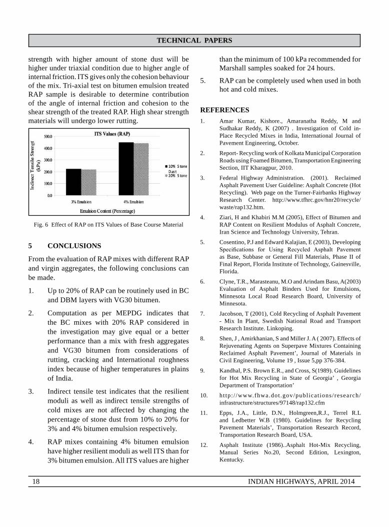
Compressive load was applied along a diametrical plane through two opposite loading strips in the resilient modulus test. This type of loading produces a relatively uniform tensile stress which is perpendicular to the applied load plane, and the specimen usually fails by splitting along the loaded plane. The test procedure is simple and the load on the Marshall Specimens is applied at the rate of 50.8 mm/min at a temperature of 25ºC. Duration of load and deformation values till breaking point is recorded. The samples were cured in an oven for 2 days at 60ºC and then soaked in water for 24 hours before the test. Results of Indirect Tensile Strength (ITS) are shown in Fig. 6. Higher emulsion content gave higher Indirect Tensile Strength. ITS values after 24 hours immersion in water are close to 215 kPa even for3%emulsioncontent,theminimumspecifiedITSbeing 100 kPa for soaked samples recommended by southAfrican specification (22)while theminimumITS value recommended for unsoaked specimens are 225 kPa. Though ITS does not indicate the contribution of higher amount of stone dust from consideration of indirecttensiletestreflectedinFig. 5 and 6, overall
TeCHNICAl pApeRs
18 INDIAN HIGHWAYS, APRIL 2014
strength with higher amount of stone dust will be higher under triaxial condition due to higher angle of internal friction. ITS gives only the cohesion behaviour of the mix. Tri-axial test on bitumen emulsion treated RAP sample is desirable to determine contribution of the angle of internal friction and cohesion to the shear strength of the treated RAP. High shear strength materials will undergo lower rutting.
Fig. 6 Effect of RAP on ITS Values of Base Course Material
5 CoNClusIoNs
From the evaluation of RAP mixes with different RAP and virgin aggregates, the following conclusions can be made.
1. Up to 20% of RAP can be routinely used in BC and DBM layers with VG30 bitumen.
2. Computation as per MEPDG indicates that the BC mixes with 20% RAP considered in the investigation may give equal or a better performance than a mix with fresh aggregates and VG30 bitumen from considerations of rutting, cracking and International roughness index because of higher temperatures in plains of India.
3. Indirect tensile test indicates that the resilient moduli as well as indirect tensile strengths of cold mixes are not affected by changing the percentage of stone dust from 10% to 20% for 3% and 4% bitumen emulsion respectively.
4. RAP mixes containing 4% bitumen emulsion have higher resilient moduli as well ITS than for 3% bitumen emulsion. All ITS values are higher
than the minimum of 100 kPa recommended for Marshall samples soaked for 24 hours.
5. RAP can be completely used when used in both hot and cold mixes.
ReFeReNCes1. Amar Kumar, Kishore., Amaranatha Reddy, M and
Sudhakar Reddy, K (2007) . Investigation of Cold in-Place Recycled Mixes in India, International Journal of Pavement Engineering, October.
2. Report- Recycling work of Kolkata Municipal Corporation Roads using Foamed Bitumen, Transportation Engineering Section, IIT Kharagpur, 2010.
3. Federal Highway Administration. (2001). Reclaimed Asphalt Pavement User Guideline: Asphalt Concrete (Hot Recycling). Web page on the Turner-Fairbanks Highway Research Center. http://www.tfhrc.gov/hnr20/recycle/waste/rap132.htm.
4. Ziari, H and Khabiri M.M (2005), Effect of Bitumen and RAP Content on Resilient Modulus of Asphalt Concrete, Iran Science and Technology University, Tehran.
5. Cosentino, P.J and Edward Kalajian, E (2003), Developing Specifications for Using Recycled Asphalt Pavementas Base, Subbase or General Fill Materials, Phase II of Final Report, Florida Institute of Technology, Gainesville, Florida.
6. Clyne, T.R., Marasteanu, M.O and Arindam Basu, A(2003) Evaluation of Asphalt Binders Used for Emulsions, Minnesota Local Road Research Board, University of Minnesota.
7. Jacobson, T (2001), Cold Recycling of Asphalt Pavement - Mix In Plant, Swedish National Road and Transport Research Institute. Linkoping.
8. Shen, J , Amirkhanian, S and Miller J. A ( 2007). Effects of Rejuvenating Agents on Superpave Mixtures Containing Reclaimed Asphalt Pavement’, Journal of Materials in Civil Engineering, Volume 19 , Issue 5,pp 376-384.
9. Kandhal, P.S. Brown E.R., and Cross, S(1989). Guidelines for Hot Mix Recycling in State of Georgia’ , Georgia Department of Transportation’
10. ht tp: / /www.fhwa.dot .gov/publ icat ions/research/infrastructure/structures/97148/rap132.cfm
11. Epps, J.A., Little, D.N., Holmgreen,R.J., Terrel R.L and Ledbetter W.B (1980). Guidelines for Recycling Pavement Materials’, Transportation Research Record, Transportation Research Board, USA.
12. Asphalt Institute (1986)..Asphalt Hot-Mix Recycling, Manual Series No.20, Second Edition, Lexington, Kentucky.

TeCHNICAl pApeRs
INDIAN HIGHWAYS, APRIL 2014 19
13. Kim,Y. and Hosin “David” Lee (2005),’ Development of Mix Design Procedure for Cold In-Place Recycling with Foamed Asphalt, Journal of Materials in Civil Engineering, ASCE, Vol 18, Issue 1.
14. Kim, Y., and Lee, H. (2007). Validation of New Mix Design Procedure for Cold In-Place Recycling with Foamed Asphalt., Journal of Material in Civil Engineering Vol 19(11), ASCE, 1000–1010.
15. Kim,Y. and Lee H .D (2011). Influence of ReclaimedAsphalt Pavement Temperature on Mix Design Process of Cold In-Place Recycling Using Foamed Asphalt, Journal of Materials in Civil Engineering , Volume 23, Issue 7.
16. Kim, Y., Lee, H. D and Heitzman M (2009), Dynamic Modulus and Repeated Load Tests of Cold In-Place Recycling Mixtures Using Foamed Asphalt, Journal of Materials in Civil Engineering , Volume 22, Issue 1.
17. Fu, P., Jones, D and Harvey, J.T, and Halles F. A(2009), ‘Investigation of the Curing Mechanism of Foamed Asphalt Mixes Based on Micromechanics Principles, Journal of Materials in Civil Engineering, Volume 21, Issue 6.
18. ASTM D 2172 (2005) Standard Test Methods for Quantitative Extraction of Bitumen from Bituminous Paving Mixtures, ASTM International, 100 Barr Harbor, USA.
19. Zaniewski, J.P. and Pumphrey, M.E. (2004), Evaluation of Performance Graded Asphalt Binder Equipment and Testing Protocol, Asphalt Technology Program, Department of Civil and Environmental Engineering, West Virginia.
20. AASHTO T 315. (2009). Standard Method of Test for Determining the Rheological Properties of Asphalt Binder Using a Dynamic Shear Rheometer (DSR), American AssociationofStateHighwayandTransportationOfficials,Washington, DC.
21. ASTM D 4123 (1982), Standard Test Method for Indirect Tension Test for Resilient Modulus of Bituminous Mixtures, Annual Book of ASTM Standards, Road and Paving Materials, Philadelphia.
22. TG 2 (2009),’A guideline for the Design and Construction of Bitumen Emulsion and Foamed Bitumen Stabilised Materials’, Asphalt Academy, CSIR Built Environment, Pretoria.
23. MEPDG- Guide for Mechanistic- Empirical Pavement Design Guide for New and Rehabilitated Pavements Structures (2004), NCHRP, Transportation Research Board, USA.
24. Kranthi Kumar K (2011). Evaluation of Design Input Parameters for Mechanistic-Empirical Pavement Design, M. Tech Thesis (Unpublished), IIT Kharagpur.

20 INDIAN HIGHWAYS, APRIL 2014
IDeNTIFICATIoN oF mAss TRANsIT CoRRIDoRs - A CAse sTuDY FoR HYDeRAbAD CITY
h.s. sathish*, h.s. jagadeesh**, r. sathya murthy**, shruthi. s***, and Phaneendra. B***
* Associate Professor** Professor*** Former Postgraduate Students
AbsTRACTHyderabad is the capital of the State of Andhra Pradesh. Hyderabad Metropolitan Area is the sixth largest metropolitan area in India. Greater Hyderabad has an estimated metropolitan population of 10 million, making it an A-1 status city. Hyderabad City is experiencing rapid growth and transportation issues have assumed critical importance.
The main objective of the study is to develop and validate an urban transport model for the Hyderabad Urban Development Authority (HUDA) area and to identify a Mass Transit corridor using the software TRANSCAD 5.0.
An advantage of Trans CAD is that it fully integrates Geographic Information System (GIS) and demand modeling capabilities required for travel demand forecasting. The model focuses on peak period conditions because these conditions include the most important recurrent congestion period and tend to guide transportation system design in the urban scenario. Peak period models provide much more accurate indications of directional travel patterns during design conditions than do daily models.
Year 2008 is considered as the base year. Transport network for the study area comprising of the road network (major arterial and some minor roads) was built. The data was collected through inventory surveys. The travel demand for the study area was estimated in terms of passenger trips by different modes.
The base year trip end models have been calibrated for total passenger travel (internal) using the validated peak periods travel patterns and using the planning variables of 2008.
The Multinomial log it model for mode choice has been calibrated by using the disaggregate travel choice data derived from observed modal share (revealed preference) with their respective travel characteristics (Time and Cost) in the base year.
The calibrated models have been used together with projected land use variables and networks to make the forecasts. The calibrated and validated model along with future planning variables and transport networks were used to predict the future travel demand in the study area. Calibrated Trip End models were used to predict the number of trips generated/attracted from/to each of the zones in the study area. Under each of the land use and network scenarios,
Car, Two Wheeler, Auto and Public Transport matrices were assigned on respective highway and transit networks iteratively tilltheflowsonthelinksstabilize.Aftereachiterationthecostandtime skims were updated and were used to re-distribute the further split of trips with respect to different modes. Once convergence was reached the transit passenger ridership (Passengers Per Hour PerDirection- PPHPD) figureswere extracted on all themajorcorridors. The corridors having high PPHPD and satisfy minimum ridership for mass transit operation are selected as the Mass Transit Corridors.
1 INTRoDuCTIoN
1.1 General
Increase in migration to urban areas is a result of inadequacies in employment opportunities, education facilities in rural areas and the development of employment opportunities in the urban areas. This increase and spatial separation between employment locations require adequate travel modes/systems to satisfy the travel needs. This is indicated by the exponential growth of motor vehicles in various States of India.
Normally cities are provided with bus systems and some cities have suburban rail system to satisfy the travel needs of the society. The demand for these modes of travel is always show increasing trends.
1.2 scope
The main objective of the study is to demonstrate the transport planning process by developing and validating an urban transport model to identify Mass Transit Corridors for the Hyderabad Urban Area. The scope of the work includes:
Transportation Engineering and Management, Department of Civil Engineering, BMS College of Engineering, Basavanagudi, Bangalore.

TeCHNICAl pApeRs
INDIAN HIGHWAYS, APRIL 2014 21
● Reviewexistingtransportationandland-use data and past studies pertaining to the Study area.
● Collectrelevantsecondarydatarequiredfor the Estimation and Projection of traffic.
● Conduct primary traffic surveys suchas Roadside Interview Survey, TrafficVolume count, speed and delay survey, limited household survey and road network inventory survey.
● Develop and validate Urban Transport(Gravity) Model for the Study Area
● Estimate directional passenger demandontheidentifiedtransitcorridors.
● Identify Mass Transit Corridors andIdentify different Transit System Alternatives.
2 sTuDY AReA
Hyderabad is currently ranked as the sixth largest urban agglomeration in the country. The Hyderabad Urban Agglomeration (HUA) consists of the Municipal Corporation of Hyderabad (MCH), 12-peripheral municipalities, Secunderabad Cantonment, Osmania University and other areas. The total area of HUA is about 778 sq. kms, including 172 sq. kms. under Hyderabad Municipal corporation Area and 419 sq. kms. under 12 Municipalities, and 187 sqkms of other areas.
2.1 Transport Characteristics
Hyderabad is experiencing rapid growth and transportation issues have assumed critical importance. Since the proportionate road length in the HUDA area hasbeenalmoststatic,trafficcongestionhasincreasedleading to endless transportation gridlocks
2.2 Road Network
Hyderabad has radial and circular form of road network development. The recent growth trend is
more in the west/south direction of Hyderabad. There are three National Highways passing through the city. They are:
● NH9(connectingVijayawadaintheeastand Mumbai in the west),
● NH 7 (connecting Hyderabad in southand Nagpur in north) and
● NH 202 (connecting Hyderabad toWarangal).
Five State Highways namely SH1, SH2, SH4, SH5 and SH6 start from the city centre and diverge radially connecting several towns and district headquarters within the State in all directions.
3 TRAFFIC CHARACTeRIsTICs
Major transportation issue faced is the numerous commuters getting into the central core (MCH area) from its hinterland through a high capacity radial network with the low capacity carriageway in the core area being unable to accept the influx of theseflowsleadingtotrafficconstrictions.Themajorareasoftripattractionsareidentifiedfortheanalysis.Peakhourflowonmajortravelcorridorismorethan9000passenger car units. The present average speed is just 12 km per hour and it is still likely to reduce if there is no improvement in the situation. The high volume corridorsidentifiedbasedonthesurveys.
3.1 public Transport system
Public Transport System (PTS) in Hyderabad is primarily road-based bus transport, until the recent addition of rail-based Multi Modal Transit System (MMTS) train services in 2003. The current mode share of public transport in the city of Hyderabad is about 42% of the estimated 71 lakh person trips per day. APSRTC buses capture about 98.3% of all the trips made by public transport whereas MMTS serves the remaining 1.7% of commuting passengers. The total share of public transport is less than 44% against the minimum desired 80%, as per the guidelines issued by the Ministry of Urban Development, GoI in 1998. Bus Transport.

TeCHNICAl pApeRs
22 INDIAN HIGHWAYS, APRIL 2014
Currently, the city division ofAPSRTC has a fleetsize of 2,800 buses and operates 2,669 schedules per day, making more than 36,000 trips across the city, covering 7.1 lakh vehicle kilometers each day. While the mode split of APSRTC is around 3.5%, the modal split share caters to more than 42%. This is shown in Fig. 1.
Fig. 1 Vehicle Type and Mode Share (Source: APSRTC-2001)
Thefleetsizeandpatronageforthepastsevenyearsfrom 1995 to 2001 are given in Table 1. It can be observed that the patronage of buses has remained stable over the years even though the fleet size isincreased over the years. The important reason for this could be deteriorating service especially in the peak hours and a concomitant proliferation of seven seated Para transit modes providing convenient accessibility.
Table 1 Fleet and Number of passengers Carried
Year bus Fleet
occupancy Rate
No of passengers Carried per Day
in millions1995-96 2018 74 2.9811996-97 2122 75 3.1771997-98 2217 69 3.0541998-99 2328 70 3.253
1999-2000 2425 63 3.052000-2001 2480 58 2.8722001-2002 2605 59 3.068
Average Annual growth (%)
4.3 0.5
3.2 para Transit
The para-transit operators, mainly in the form of auto-rickshaws (3-seater and 7-seater) have mushroomed in the recent years to capture the peak hour demand and are emerging as unhealthy competitors to the APSRTC buses. A total of 80,000 auto-rickshaws ply on the city roads and cater to an estimated 10% of the 71 lakh person trips each day. While a proper integration of para-transit can actually complement the bus system, this has not happened due to the much unorganized nature of the sector with too many independent owners of auto rickshaws. The high degree of maneuverability of the auto rickshaws and frequent stopping on the carriageway to serve the passengers have resulted in thesevereproblemtosmoothflowof road traffic inthe city.
3.3 multi modal Transport system (mmTs)
The local train operations in the city have been introduced under the banner of MMTS in a limited way as a joint venture between GoAP and Ministry of Railways (MoR) in 2003. The current network extends to about 50 kilometers with 26 stations, served by 10 rakes. In spite of the severe demand for faster public transport modes, MMTS train operates very much below the actual carrying capacity and cater to about 35,000 passenger trips per day. This is primarily because of very low frequency of about 40 to 80 minutes (headway) between two successive days. This is primarily because of very low frequency of about 40 to 80 minutes (headway) between two successive.
4 TRANspoRTATIoN sTuDIes AND ANAlYsIs
The objective of the primary traffic surveys is toobtain current demand on the transportation network of the city, operating characteristics of the urban transport systems, socio-economic profile of thecity’s population, and characteristics of various elements of urban transport. The following surveys were undertaken to develop/update the traffic andtransportation data for the study: Inner and Outer Cordon Survey, Road Side Interview, Speed & Delay,

TeCHNICAl pApeRs
INDIAN HIGHWAYS, APRIL 2014 23
Road Network Inventory and Household Interview. The standard survey formats for all the surveys wereused.Thefindingsaredetailedinthefollowingsections.
4.1 Traffic Studies
Traffic studies were conducted at 13 locations asshown in Fig. 2 and summary is given in Table 2. During eight hours of a normal day, a total of about 6,01,935 vehicles (about 6, 52,164 PCU) move in and out through the cordon points. Of which Vijayawada road carries highest volume of traffic equivalent to72,967 PCU per eight hours of a normal day. In the compositionoftraffic,thepercentoftwowheelersarepredominant on all the selected corridors followed by auto rickshaws and cars as indicated in Fig. 3.
Fig.2TrafficStudyArea
Table 2 Details of 8-Hour Traffic at Selected Locations
sl. No. Name of the Road Total 8 hr Traffic in pCu
1 Bollaram Road 124132 Mumbai Road 1 398563 Bowenpally Road 368194 Chikkadapally Road 505985 ECIL X Road 644936 Kaldikali X Road 271397 Mumbai Road 2 654038 Osman Sagar Road 412959 Panjagutta Road 6244510 Mumbai Road 3 6540311 Vijayawada Road 72967
Fig.3AverageCompositionofTraffic
4.2 Peak Hour Traffic
ECIL X Road is carrying maximum peak hour traffic of 12,219 PCU followed by 11,799 PCUat Vijayawada Road and 10,945 PCU at Mumbai road2andMumbairoad3.Thepeakhourtrafficforthe selected locations are given in Table 3.
Table 3 Peak Hour Traffic of all Survey Locations
Road Name peak Hour peak Hour Vehicles
peak Hour pCu
Bollaram Road 6.00-7.00 2598 2624
Mumai Road 1 8.00-9.00 8293 8775
Bowenpally Road 5.30-6.30 5646 6633
Chikkadapally Road 4.00-5.00 9988 9745
Ecil X Road 4.30-5.30 8904 12219
Kaldikali X Road 8.15-9.15 4033 5646
Malakpet Road 9.15-10.15 8928 9480
Medak Road 8.00-9.00 9410 10580
Mumbai Road 2 5.00-6.00 10127 10945
Osman Sagar Road 9.15-10.15 7472 7406
Panjagutta Road 8.00-9.00 10856 9947
Mumbai Road 3 5.00-6.00 10127 10945
Vijayawada Road 8.00-9.00 10634 11799
4.3 origin and Destination survey
This survey was conducted to find-out the trip pattern, trip frequency and trip purposes of the Hyderabadcitytraffictherebypassengertravelpatternis determined.

TeCHNICAl pApeRs
24 INDIAN HIGHWAYS, APRIL 2014
The zoning scheme has been designed based on the municipal ward boundaries so that the zoning system is in coherence with those adopted by the local planning bodies and those by used the past studies. The zone system of study area comprised of 85 internal zones and 6 external zones outside Hyderabad city area, making a total of 91 zones.
5 TRIp FReQueNCY
Road Name peak Hour peak Hour
Vehicles
peak Hour
pCu
Bollaram Road 6.00-7.00 2598 2624
Mumbai Road 1 8.00-9.00 8293 8775
Bowenpally Road 5.30-6.30 5646 6633
Chikkadapally Road 4.00-5.00 9988 9745
ECIL X Road 4.30-5.30 8904 12219
Kaldikali X Road 8.15-9.15 4033 5646
Malakpet Road 9.15-10.15 8928 9480
Medak Road 8.00-9.00 9410 10580
Mumbai Road 2 5.00-6.00 10127 10945
Osman sagar Road 9.15-10.15 7472 7406
Panjagutta Road 8.00-9.00 10856 9949
Mumbai Road 3 5.00-6.00 10127 10945
Vijayawada Road 8.00-9.00 10634 11799
The average trip frequency distribution is as shown in Fig. 4. Analysis of trip frequency shows that daily trips are more with 50% followed by multiple trips a day and weekly trips having a frequency of 30% and 10% respectively.
Fig. 4 Trip Frequency
6 JouRNeY puRpose
Analysis of purpose of trips revealed that the average work trips are 42% followed by Business trips 37% and other trips with 13%. The average journey purpose distribution is as shown in Fig.5.
7 oCCupANCY RATe
The average occupancy rates of various modes are as shown in Table 4. The occupancy of car, auto and two wheelers is 3.2, 3.6, 1.5 and bus 62 respectively.
Fig. 5 Purpose Wise Distribution of Trips
Table 4 occupancy Rate
Vehicle Type Avg. occupancyTruck 1.5MAV 3.9LCV 1.0Car 3.2Auto-rikshaw 3.6Two wheelers 1.5Bus 62
8 speeD AND DelAY suRVeY
The purpose of this survey is to evaluate the existing speeds on the network and to use the data in the calibrationofthespeedflowcurves.Thedataisusedindevelopingthespeedflowrelationshipsinbuildingthe Transport Model and to validate journey speeds predicted by the transport model.The surveys were conducted during peak and off-peak hours on any normal day on selected major corridors. The delays and corresponding causative factors at intersections/ major activity centers etc. were collected to identify major bottlenecks on the road.

TeCHNICAl pApeRs
INDIAN HIGHWAYS, APRIL 2014 25
9 RoAD NeTWoRK INVeNToRY suRVeY
A database on the road features is collected by inventorying selected roads in the study area. The database is used in developing the base year network facilitating both qualitative and quantitative evaluationofthepresentsufficiencyofroadnetworksvis-à-vis existing standards and usage pattern. The following data were collected during the field inventory survey: Effective Road width, No of lanes, Availability of median, shoulder etc. and Encroachments along the city roads. Based on the cross sectional measurements taken at 30 locations on the road network. About 42% of the primary road length has carriage way width between 21.0-28.0 m and 50% of the secondary road length has carriage way width between 5.5-7.0 m. Classifying these roads by type of the carriage way, it is observed that 85% of the primary road network have divided carriageway, out of which most of the roads are 6 lane divided carriageway. About 98% of the secondary road network have undivided carriage way, from which most of the roads are 2 lane undivided carriage way.
10 summARY oF HHI suRVeY FINDINGs
Thefigureonvariousplanningparametersinrespectof the city as per the survey are given in Table 5.
11 bAse YeAR moDel DeVelopmeNT
11.1 Introduction
A travel Demand model for Hyderabad has been calibrated for evaluating existing travel conditions and forecasting future travel demand. The model analyzes the present and future land use patterns to estimate the origins and destinations of trips. It then assigns these trips to different travel routes and travel modes based on the type and quality of the transportation network.
Table 5 summary of HHI survey
parameters Year 2006No. of households for HHI 1000Average family size 3.25
Per capita trip ratePCTR(all) 0.963PCTR(motorized) 0.827Household monthly income in Rs. 9060
Average vehicle ownership/HHTwo wheeler 1.4Car 0.54
Mode distribution (%)Walk 10.2Pedal Cycle/Pillion Rider 2.1Scooter/mc 35.3Public transport 42.3Car/van/jeep 4.5Auto 5.6
Travel Demand model can be used for testing different scenarios before implementing the projects. For example, one can see the impact of adding mass transport like BRT. Similarly impact on transportation network due to changes in the land use patterns can be analyzed. The broad framework for the transport modeling for Hyderabad city is given in the Fig. 6.
Fig. 6 Framework for Transport Modeling
Several software programs are available for developing travel demand models. The Hyderabad transport model

TeCHNICAl pApeRs
26 INDIAN HIGHWAYS, APRIL 2014
has been developed using Trans CAD (a state-of-the-art Travel Demand Modeling software).
11.2 model structure
The model is based on a conventional 4-stage transport model approach. Once the model is calibrated, it can be used to predict the future travel patterns under different land use transport scenarios.The model is responsive to:
● Streetcongestion,travelcosts,availabilityof competing transport modes including other Public Transport systems and the growth of the city.
● Generalized costs that include out ofpocket costs i.e. fare, vehicle operating cost etc. and perceived user costs such as value of travel time, cost of waiting time for transit etc.
The model focuses on morning journey to work peak period conditions. Peak period models provide much more accurate indications of directional travel patterns during design conditions than do daily models. However, the daily traffic forecasts can beestimated using peak-to-day expansion factor which isobtainedfromthetrafficsurvey.Fromthesurveysit was observed that the city morning peak hour is during 8.00 AM to 9.00 AM. So the model was built for this duration.
11.3 planning period
The year 2008 is taken as the base year. Demand forecasting on the network and on any proposed mass transit system is required over a 25 year period. In order to analyze the travel demand in the study areaandestimate the likely trafficpatronageonanyproposed system, all relevant data have been collated for the base year 2008, the horizon year 2031 and the two intermediate years (2011 & 2021).
11.4 modes
The modes that are modeled in the study include two wheeler, car, auto rickshaw and public transport. The
Non-Motorized Transport and Commercial vehicles were considered as a Preload.
11.5 Network Development
Transport network developed for the model comprises of two components: Highway Network for vehicles and Transit Network for public transport system i.e. buses, rail and any new public transportation system. Each of the networks is described in detail below.
11.6 Highway Network
The coded highway network for the study area represents the nodes (intersections), linkages between them and characteristics of the street and highway system in order to support estimation of trafficvolumes, speeds and vehicle travel times on individual links of the system plus zone-to-zone travel times. The road network was properly connected to all the zone centroids by means of centroid connectors. Study area Zoning Map shown in Fig. 7.
Fig. 7 Study Area Zoning Map
The BPR (Bureau of Public Roads) formulation is used as link performance function. The BPR function, given below, relates link travel time and the volume/capacity ratio:
t = tf [1 + α (V/C)β] ... 1

TeCHNICAl pApeRs
INDIAN HIGHWAYS, APRIL 2014 27
Where,
t = Congested link travel time,
tf = Linkfree-flowtraveltime,
V = Link volume,
C = Link capacity,
α,β = Calibrationparameters
12 TRANsIT NeTWoRK
The transit network represents the connectivity, head ways, speeds and accessibility of transit services. Hyderabad’s bus transport system is included in the model’s transit network. The transit routes are specifiedasthoseusingthetransportlinksandhavingstops/stations at determined locations. The access to the stops/stations from zone centroids and other nodes is provided either by existing highway links or by definingexclusivewalk links.About120bus routesare operated in the study area. Information on the same was collected and coded in to the system. Fare structure and frequency for each of these services are also included.
13 bAse YeAR TRAVel (2008) pATTeRN
We have synthetic trips using trip distribution and mode choice models from past studies. The trip matrices are significantly updated using fresh householdsurvey and roadside interview. The external trips for the car, two wheeler, auto and public transport were constructed based on the O-D survey conducted at the outer cordon. The trip matrices thus derived were then compared with the per capita trip rate for study area derived from the household interview data. The results of the travel demand estimation for base year and trip rate analysis is summarized in the Table 6.
14 AssIGNmeNT AND obseRVeD o-D VAlIDATIoN
These mode-wise base matrices were assigned on the network. The assigned volume on the network was compared with the observed volume on the screen
lines adopted for the study area. Table 7 gives the comparisonofassignedflowswiththetrafficvolumeobserved on the road. Fig. 8 shows the desire line diagram for the study area.
Table 6 summary of estimated base Year (2008, peak Hour Travel Demand
sl. No mode Internal Trips
external Trips
Total Trips
1 T/W Passengers
194377 36772 231149
2 Car Passengers
52654 5063 57717
3 Auto Passengers
35795 3322 39117
4 Public Transit Passengers
299358 13668 313025
Table 7 Results of observed oD Validation on screen lines
mode Hyderabadobserved Assigned % Difference
T/W 30932 32427 -5%CAR 20341 19199 6%
AUTO 18153 16738 8%PT (Buses) 10094 11120 10%
Fig. 8 Desire Line Diagram
15 bAse YeAR ResulTs
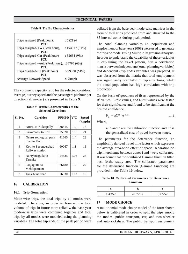
Thetrafficcharacteristicsofthestudyareaintermsofaverage network speed, volume to capacity ratio, etc. are given in Table 8.
TeCHNICAl pApeRs
28 INDIAN HIGHWAYS, APRIL 2014
Table 8 Traffic Characteristics
The volume to capacity ratio for the selected corridors, average journey speed and the passengers per hour per direction (all modes) are presented in Table 9.
Table 9 Traffic Characteristics of the selected Corridors
sl. No. Corridor ppHpD V/C speed (kmph)
1 BHEL to Kukatpally 38515 1.9 18
2 Kukatpally to Koti 75320 1.8 21
3 Nehru zoological park road to Koti
41665 1.4 22
4 Koti to Secunderabad Railway station
60067 1.1 18
5 Narayanaguda to Tarnaka
54835 1.06 26
6 Panjagutta to Mehdipatnam
66480 1.2 22
7 Tank bund road 76330 1.63 19
16 CAlIbRATIoN
16.1 Trip Generation
Mode-wise trips, the total trips by all modes were modeled. Therefore, in order to forecast the total volume of trips in future more reliably, the base year mode-wise trips were combined together and total trips by all modes were modeled using the planning variables. The total trip ends of the peak period were
collated from the base year mode-wise matrices in the form of total trips produced from and attracted to the 85 internal zones during peak period.
The zonal planning variables i.e. population and employment of base year (2008) were used to generate the trip end models using Multiple Regression Analysis. In order to understand the capability of these variables in explaining the travel pattern, first a correlationmatrix between independent (zonal planning variables) and dependent (trip ends) variables was prepared. It was observed from the matrix that total employment was significantlycorrelated to tripattractions,whilethe zonal population has high correlation with trip production.
OnthebasisofgoodnessoffitasrepresentedbytheR2 values, F-test values, and t-test values were tested fortheirsignificanceandfoundtobesignificantatthedesiredconfidence.
Fi–j = aCbi–j e–cCi-j ... 2
Where,
a, b and c are the calibration function and C’ is the generalized cost of travel between zones.
The parameters for the deterrence function, an empirically derived travel time factor which expresses the average area-wide effect of spatial separation on trip interchange between zones i and j were calibrated. ItwasfoundthatthecombinedGammafunctionfittedbest forthe study area. The calibrated parameters for the deterrence function (Gamma Function) are provided in the Table 10 below.
Table 10 Calibrated parameters for Deterrence Function
a b c1.4357 -0.7282 0.0557
17 moDe CHoICeA multinomial mode choice model of the form shown below is calibrated in order to split the trips among the modes, public transport, car, and two-wheeler and auto rickshaw. The public transport assignment

TeCHNICAl pApeRs
INDIAN HIGHWAYS, APRIL 2014 29
module shall achieve the modal split among the public-transport modes i.e., Bus, and Rail. Utility functions (VM) for each mode were calibrated using the disaggregate person trip and mode choice data derived from the observed o-d, travel time and travel cost for each individual.
VM=αTTM+βTCM ... 3
Where,
TTM - Travel Time by Mode M
TCM - Travel Cost by Mode M
αandβaremodalcalibrationparameters
The information on the alternate modes, i.e., travel time and travel cost, available to user, was generated from the time and cost skims obtained in public transport and highway assignment procedures. The calibrated parameters are given in Table 11.
Table 11 Calibrated mode Choice parameters
mode α βTwo Wheeler 0.028827 -0.039631
Car -0.007659 -00011820Auto 0.008080 -0.0059658
Public Transport
0.013137 0.046076
17.1 Validation- Average Trip length
To assure the reliability of the model, the average trip length by mode from the model is compared with the results obtained from the Household interview survey. It was observed that the average trip length from the model is closely matching with House hold interview survey. Table 12 presents the comparison of average trip length obtained from the model and the House Hold Survey.
Table 12 mode wise Trip length
mode model Household surveyPV 9.34 9.01PT 11.40 10.98
18 TRAVel DemAND FoReCAsT
The strategic Urban Travel Demand Model developed under this study is used to predict the travel patterns and modal shares in the horizon year i.e. 2031 under respective land-use and transport network scenarios.
Trip End models have been used to predict the number of trips generated from and attracted to each of the zones in the study area. Projected trip ends along with the network options in the future were provided as inputs to the distribution and modal split models to arrive at future trip matrices for Car, Two Wheeler, Auto-rickshaw and Public Transport.
18.1 Horizon Year land-use scenario
The projected population and employment for 2011, 2021 and 2031 were used for estimating trip ends in the corresponding years. The population and employment projections are given in Table 13 and Table 14 respectively.
Table 13 projected employment in the study Area
Name of the Area
projected employment in the study Area (lahks)
2007 2011 2021 2031
HUDA 27.696 28.775 40.941 55.123
Table 14 projected employment in the study Area
Name of the Area
projected employment in the study Area (lahks)
2007 2011 2021 2031
HUDA 74.028 76.912 102.085 120.928
19 TRAFFIC FoReCAsT uNDeR Do-NoTHING sCeNARIo
The summary of the projected peak hour passenger travel demand in the study area and the corresponding modal share are given in Table 15.

TeCHNICAl pApeRs
30 INDIAN HIGHWAYS, APRIL 2014
Table 15 Traffic Characteristics
Trips assigned (Peak hour), : 582184PCU
Trips assigned-TW (Peak hour), : 194377 (33%)PCU
Trips assigned-Car (Peak hour) : 52654 (9%)PCU
Trips assigned –Auto (Peak hour), : 35795 (6%)PCU
Trips assigned-PT (Peak hour) : 299358 (51%)PCU
Average Network Speed : 19 kmph
The traffic characteristics of the study area areextracted from the model in terms of average network speed, volume to capacity ratio, etc. and the volume to capacity ratio for the major roads; average journey speed and the passengers per hour per direction (All modes) are presented in Table 16 and 17 respectively.
Table 16 summary of Forecast of peak Hour passenger Demand
Year mode Internal external percentage
2011 Two Wheeler 238085 40449 38%
Car 64050 7088 10%
Auto 42596 4153 7%
Public Transport
281160 16402 45%
Total 625891 68092 100%
2021 Two Wheeler 385133 52584 41%
Car 109512 10278 12%
Auto 81354 5398 9%
Public Transport
364476 19846 39%
Total 940475 88106 100%
2031 Two Wheeler 525569 68359 42%
Car 183361 14903 15%
Auto 133319 7018 11%
Public Transport
395602 24014 32%
Total 1237852 114293 100%
Table 17 Major Road Traffic Forecasts – 2031- Do Nothing scenario
sl. No. Corridor ppHpD V/C speed (kmph)
1 BHEL to Kukatpally 65090 3.9 92 Kukatpally to Koti 113733 3.6 123 Nehru Zoological
Park Road to Koti68747 2.9 14
4 Koti to Secunderabad Railway station
83493 4.6 10
5 Narayanaguda to Tarnaka
86639 2.6 8
6 Panjagutta to Mehdipatnam
108362 4.1 11
7 Tank Bund Road 110679 3.6 9
19.1 Choice of CorridorWhile selecting the corridors, the following issues were considered: Better Access to land-use, Connectivity to primeareasandothertransportmodes,Userbenefitslike saving on fuel, Minimal travel time, and Minimal land acquisition, Minimal conflict with existingand proposed structure and Better integration with proposed developments.
19.2 Ridership ForecastThe carrying capacities – expressed in terms of PPHPD, on the sections of major corridors based on trafficforecastfromtheTransCADmodelaregivenin the Table 18 below:
Table 18 Ridership (ppHpD) Forecast
No. Corridor 2011 2021 20311 BHEL to Kukatpally 41981 53536 650902 Kukatpally to Koti 80330 97032 1137333 Nehru zoological park
road to Koti45197 56972 68747
4 Koti to Secunderabad Railway station
63123 73308 83493
5 Narayanaguda to Tarnaka
58983 72811 86639
6 Panjagutta to Mehdipatnam
71943 90152 108362
7 Tank bund road 80810 95744 110679

TeCHNICAl pApeRs
INDIAN HIGHWAYS, APRIL 2014 31
The numbers are based on the normal scenario and indicate that a mass transit system facility is needed. However, with a policy intervention, according due allocation of anticipated trips with a greater share for mass transport modes as suggested in the National urban transportPolicy, thePPHPDon the identifiedcorridorsare estimated as shown in the Table 18.
20 DIsCussIoN AND CoNClusIoN
20.1 Discussion● By theyear2031Hyderabadcity isprojected
to have a population of about 12.1 million with employment of 5.5 million. This translates into a travel demand of approximately 12.37 lakhs trips during peak hours of the day.
● It is observed that TwoWheelers contributesabout 30% followed by Auto rickshaws with 19% and Cars with 17% during peak hour.
● V/CratioonallthemajorroadsinHyderabadCityexceeds1.0 indicating trafficcongestion,low speed and high delays. The average network speed in the base year (2008) and Horizon Year (2031) under the Do-Nothing Scenario is 19kmph and 10kmph respectively.
● TheanalysisoftheHouseholdInterviewSurveyindicates that average family size of Hyderabad City is 3.25, the overall Per Capita Trip Rate (PCTR) is 0.963 and the motorized Per Capita Trip Rate (PCTR) is 0.827.
● The comparison of assigned flows with thetraffic volume observed on selected road anddifference in vehicle-wise PCU at the screenline was observed to be within the acceptable range of ± 15%.
● There exist a linear relationship betweenPopulation and Trip Production and Trip Attraction. The co-efficient of correlation R2value was found to be 0.629 for Trip Production and 0.538 for Trip Attraction.
● The base desire lines connecting the originpoints with the destinations are shown in Fig.8. The widths of these desire lines are proportional to the number of trips in both the directions during the peak hour.
● The mode-wise average trip length from themodel is compared with theresults obtained from the Household Interview Survey in order to assure the reliability of the model. It was observed that the average trip length from the model is closely matching with House hold interview survey.
● Traffic Characteristics such as PPHPD, V/Cratio and Speed (kmph) of major road network for the base year (2008) and the horizon year (2031) are presented.
● The summary of the projected peak hourpassenger travel demand in the study area and the corresponding modal share is given in Table 15.
● The current public transport captures about50% of the total trips. Whereas in the horizon year 2031 public transport captures about 32% of the total trips. This is due to the increase of private vehicle trips (Cars and Two Wheelers).
● In the absence of a mass transport systemtrafficcongestionandmobilitywillcontinuetodeteriorate over the years.
● TheidentifiedMassTransitCorridorsareshownin Table 3. The ridership forecast in terms of PPHPD is presented in Table 18.
Following conclusions can be drawn from discussions:
i. The calibrated Urban Travel Demand Modelcanbeused topredict the trafficand transport supplies in the horizon years in the study area.
ii. Thereexist a linear relationship between Population and Trip Production and Trip Attraction. Hence there exist reasonably good correlation between dependent and independent variables.
iii. Calibrated Trip End Models can be used for forecasting the travel characteristics in the study area as well as to understand the impact of any proposed improvements and Mass Transit System in the study area.
TeCHNICAl pApeRs
32 INDIAN HIGHWAYS, APRIL 2014
iv. The maximum Peak Passenger Hourly Volume Per Direction (PPHPD) on the identifiedtransitcorridorsisintherangemodel with Table 3 it can be concluded of 30,000 to 80,000. Hence by comparing the PPHPD obtained from travel demand that all the seven identified transit corridorswarrant a Mass Transit System.
ReFeReNCes1. KadiyaliL.R,(2002),”TrafficEngineeringandTransport
Planning”, Third Edition, Khanna Publishers, New Delhi.2. Khanna S.K. and Justo C.E.G, (2007) “Highway
Engineering”, Eight Edition, Nem Chand & Bros, Roorkee.
3. Syed Anisuddin, (1998), “Mass Transit System Planning AndSchedulingForAnIdentifiedCorridorIncorporatingOn-Line Congestion Effects Through Optimization Techniques”, October, Department of Civil Engineering, Regional Engineering College, Warangal, (Un Published PhD Thisis).
4. John Bates, (2008), “History of Demand Modelling”, Handbook of Transport Modelling, Vol.1, Elsevier.
5. Papacostas, C.S. and Prevedouros, (2001), “Transportation Engineering and Planning”, University of Hawaii, Third Edition, Prentice Hall.
6. Edward A. Beimborn, (2006), “Inside the Black box, Making Transportation Models Work for Livable Communities”, Center for Urban Transportation Studies University of Wisconsin-Milwaukee, June.
7. Prem Pangotra and Somesh Sharma, (2006), “Modeling Travel Demand for Metropolitan City”, http://www.iimahd.ernet.in/assets/snippets/workingpaperpdf/2006-03-06pangotra.pdf.
8. Markus Friedrich, (2004), “Prospects of Transportation Modelling”, Proceedings of 2nd International Symposium Networks for Mobility, Stuttgart, University Stuttgart.
9. Chandra R. Bhatet al, (2007), “Passenger Travel Demand Forecasting”, A1C02: Committee on Passenger Travel Demand Forecasting, TRB.
10. City Development Plan, Jawaharlal Nehru National Urban Renewal Mission (JNNURM), (2006), Municipal Corporation of Hyderabad.
11. Wilbur SmithAssociates, (2008), “Study onTraffic andTransportation Policies and Strategies in Urban Areas in India”, Ministry of Urban Development –India.
12. WilburSmithAssociates,(2007)“ComprehensiveTrafficand Transportation Study for the Town of Nellore”, Andhra Pradesh Urban Services for the Poor (APUSP).

INDIAN HIGHWAYS, APRIL 2014 33
lAboRAToRY eVAluATIoN FoR THe use oF mooRum AND GANGA sAND IN WeT mIX mACADAm uNbouND bAse CouRse
g.d. ransinchung r.n*, Praveen Kumar**, Brind Kumar***, aditya Kumar anuPam**** and arun PraKash chauhan*****
* Asstt. Professor, E-mail: [email protected]** Professor, E-mail: [email protected]*** Asstt. Professor, Department of Civil Engineering, IIT-BHU, Varanasi, E-mail: [email protected]**** Ph.D. Scholar, E-mail: [email protected]***** M.Tech. Student, E-mail: [email protected]
AbsTRACTMoorum is fragmented weathered rock naturally occurring with varying proportions of silt and clay. It is considered as a low grade marginal material for road construction by codes and has generally low bearing capacity and high water absorption value in comparison to conventional aggregates. It finds applicationin the construction of Water Bound Macadam as binders at such locations where it abundantly available within short hauling distances. Quality of moorum varies significantly from onelocation to another in terms of its crushing and impact value, grain size, clay and deleterious content. Sukrut in Sonebhadra district of Uttar Pradesh has abundant good quality moorum. This gravelly material has been found to be well graded and has CBRvalue of 40%, ten percent fines value of 56 kN, crushingand impact values were less than 30%. Ganga sand is locally availablefinesandatVaranasi.Therefore,thepresentworkseeksto study the suitability of using moorum and local Ganga sand by part replacing the stone dust proportion of conventional Wet Mix Macadam (WMM) mix. Secondly, ordinary Portland cement was used as stabilizer with moorum in proportions varying from 3% to 9% to study its suitability as WMM layer. A total of seven WMM mix proportions were considered including the conventional mix. Results show that incorporation of Ganga sand to replace 20% proportion of stone dust of conventional WMM mix was found to improve the CBR value from 121% for conventional mix to 169%. This was while the same level of replacement with moorum had decreased the CBR value of WMM mix to a value of 94%. However, when moorum was used with OPC in incremental rate of3%,significantincreasewasobservedfordrydensity,CBRandunconfinedcompressivestrength.Thiswasachievedatthecostofloss of permeability of the mix. Moorum admixed with 3% OPC is preferable on account of being comparable to the conventional WMM mix in terms of CBR value, retaining its permeability and affording maximum cost savings. Cost comparisons show significantsavingsonadmixingascomparedtotheconventionalWMM mix.
1 INTRoDuCTIoN
Most developing countries are witnessing a steep rise in consumption of aggregates to support their
road construction activities. Demand of good quality crushed aggregates is on a continuous rise against the backdrop of its ever rising costs and depleting availability. Newer quarries are continuously being established with increasing lead distances from the consumption points under growing environmental concerns. Locally available materials with abundant availability at cheaper cost may help tide over the situation. Material engineers of the highway industry are continuously looking for such alternative materials that may substitute the use of conventional aggregates without compromising on strength and durability while causing a reduction in the construction costs.
The unbound granular base is a structural component oftheflexiblepavementthatplaysanimportantrolein imparting stability and durability to the upper layers [Darter & Von Quintus, 1997]. It plays a major role in spreading the wheel loads incident on the surface in a manner that the stresses transmitted to the sub-base and sub-grade do not exceed their bearing capacity [Zagreb, 1989; Brandl, 1977]. A well-designed and constructed base increases the foundation support, helps reduce stresses and improves load transfer. All these leads toasignificant reduction in thecrackingand faulting potential of the pavement [Barber & Sawyer, 1952]. Construction of a permeable base rapidly removes water from the pavement structure [US Corps Engineering Manual EM1110-2-1906, 1970].
India faces an increasingly urgent need for building and expanding its road infrastructure at the earliest. The increasing gap between the supply and demand of conventional good quality crushed aggregates
Department of Civil Engineering, IIT-Roorkee
Department of Civil Engineering, IIT-Roorkee

TeCHNICAl pApeRs
34 INDIAN HIGHWAYS, APRIL 2014
is already evident. A maximization of alternate sustainable materials as partial replacement of conventional crushed aggregates would play a vital role not only in achieving the quantity requirements for speedyconstruction,butalsosignificantimprovementsin quality and economy under sustained scientificinnovations. The demand for construction aggregates in India was 1.1 billion metric tons in 2006, making the country the third biggest aggregates market in the Asia-Pacific region and fourth largest marketin the world after China, the US and Japan (www. freedoniagroup.com, 2007). Considering the highway sector alone, about 15,000 tonnes of aggregates are required per kilometer (www.equipmentIndia.com).
Moorum is fragmented weathered rock naturally occurring with varying proportions of silt and clay. It is considered as a low grade marginal material for road construction by codes. It has generally low bearing capacity and high water absorption value in comparison toconventionalaggregates.Itfindsapplicationintheconstruction of Water Bound Macadam as binders at such locations where the same is abundantly available in short hauling distances. Quality of moorum varies significantly from one location to another in termsof its crushing and impact value, grain size, clay and deleterious content. Its application in Wet Mix Macadam (WMM) unbound base course becomes a matter of study for its eventual use.
Secondly, stone dust is gradually becoming costlier due to consistent rise in its demand. Its application is necessary to achieve the desired gradation of WMM as per MoRT&H (IV Revision). Several attempts have been made earlier to substitute or partially replace the same with other similar type of material. Local sand is also a fine material and studies are necessary todetermine its potential for replacing stone dust.
The present laboratory investigation was conducted with a view to evaluate Ganga sand and moorum being abundantly available and cheap local material in and around Varanasi district of the state of Uttar
Pradesh in India. It seeks to study the suitability of using moorum and local Ganga sand by part replacing the stone dust proportion of conventional Wet Mix Macadam (WMM)mix as per the specifications setout in the Ministry of Road Transport and Highways (MoRT&H), IV Revision, envisaging comparable material quality and overall reduction in construction cost. Secondly, Ordinary Portland Cement (OPC) was used as stabilizer with moorum in proportions varying from 3% to 9% to study its suitability as WMM layer.
2 mATeRIAls useD
2.1 moorum
Moorum was collected from Sukrut in Sonebhadhra district of Uttar Pradesh. This quarry is located at a distance of about 40 km from Varanasi on Varanasi-Shaktinagar road. Its physical properties are shown in Table 1.
Table 1 physical properties of moorum
physical properties Results
Aggregate crushing value, % 28.0
Aggregate impact value, % 27.0
Specificgravity(IS:2720,Part-3) 20 mm 10 mm
2.6172.620
Water absorption (IS:2720, Part-2), % 20 mm 10 mm
2.8903.896
Tenpercentfinesvalue(BS:812,Part-111),kN 56
Liquid limit (IS:2720, Part-5), % 35
Plastic limit (IS:2720, Part-5), % 25
Plasticity index (IS:2720, Part-5), % 10
Maximum dry density (IS:2720, Part-8), g/cc 2.1
Optimum moisture content (IS:2720, Part-8), % 8.05
Coefficient of permeability (k) (IS:2720, Part-17),cm/sec
1.24x10⁻³
California bearing ratio (IS:2720, Part-16), % 40

TeCHNICAl pApeRs
INDIAN HIGHWAYS, APRIL 2014 35
2.2 Ganga sand
Local Ganga sand collected from Varanasi having fineness modulus of 1.95 was used. Its physicalproperties are presented in Table 2.
Table 2 physical properties of Ganga sand at Varanasi
physical properties Results
Grain size distribution (IS:2720, Part-4)Gravel, %Sand, %Silt, %Clay, %
--65.0030.005.00
Specificgravity(IS:2720,Part-3) 3.02
Water absorption (IS:2720, Part-2), % 1.06
Plasticity index (IS:2720, Part-5), % Non-plastic
California bearing ratio (IS:2720, Part-16), % 80.0
2.3 Crushed stone Aggregates and stone Dust
Crushed stone aggregates and stone dust were collected from Dalla in Sonebhadhra district of Uttar Pradesh. Its lead from Varanasi is about 125 km. Their physical properties are shown in Table 3.
Table 3 physical properties of Crushed Aggregates and stone Dust
physical properties Crushed Aggregates stone Dust
40 mm NmAs
20 mm NmAs
10 mm NmAs
SpecificgravityasperIS:2386 (Part-3)
2.698 2.672 2.615 2.600
Aggregate crushing value as per IS:2386 (Part-4), %
18 -
Aggregate impact value as per IS:2386 (Part-4), %
16 -
Combinedflakinessandelongation indices as per IS:2386 (Part-4), %
35 38 45 -
Los Angeles abrasion value as per IS:2386 (Part-4), %
17 18 21 -
Water absorption as per IS:2386 (Part-3), %
0.75 0.80 0.90 1.10
2.4 ordinary portland Cement
Ordinary Portland Cement (OPC) 43 grade conforming toIS:8112wasusedasastabilizer.Itsspecificgravitywas 3.13.
3 Wmm mIX pRopoRTIoNs AND lAboRAToRY INVesTIGATIoNs
As outlined in the objectives, the study entails evaluation of abundantly available and cheap local material like Ganga sand and moorum in and around Varanasi for partial replacement of conventional crushed aggregates and stone dust for construction of Wet Mix Macadam (WMM) unbound base course as per MoRT&H specifications (IV revision). In orderto achieve this, relevant laboratory investigations like grain size analysis (IS:2720, Part-4), Proctor’s modifiedcompaction (IS:2720,Part-8),permeability(IS:2720, Part-36), California Bearing Ratio (CBR) (IS:2720, Part-16) and unconfined compressivestrength (UCC) (IS:4332, Part-5 and IS:9143) were conducted on seven set of WMM mix proportions as shown in Table 4.
The referral mix (M1) comprised of 40 mm, 20 mm, 10 mm crushed stone aggregates and stone dust proportioned at 24%, 16%, 32% and 28% respectively by weight of total mix so as to conform within the grading limits of MoRT&H (IV revision), Section 406. 20% by weight of total mix of stone dust proportion of the referral mix was replaced once with Ganga sand for the mix designation M2, and next with moorum for mix designation M3.
Another set of mixes were prepared using 100% moorum for mix designation M4. OPC as stabilizer was used to replace moorum at 3%, 6% and 9% by weight for the mix designations M5, M6 and M7 respectively.

TeCHNICAl pApeRs
36 INDIAN HIGHWAYS, APRIL 2014
Table 4 proportioning of Wmm mix Designations
mix Designation
percentage by Weight of40 mm NmAs 20 mm NmAs 10 mm NmAs stone Dust Ganga sand moorum opC
M1 24 16 32 28 - - -M2 24 16 32 8 20 - -M3 24 16 32 8 - 20
(< 9.5 mm)-
M4 - - - - - 100 -M5 - - - - - 97 3M6 - - - - - 94 6M7 - - - - - 91 9
Three set of moulds were prepared for each mix designation for Proctor’s test, permeability test, CBR and UCC tests. The tests were conducted as per the relevantstandardspecificationsinthelaboratory.Formix designations M1, M2, M3 and M4 the specimen were cast at respective OMC and tested. For mix designations M5, M6 and M7 the specimen were cast at OMC and left 7 days for curing prior to test. Curing was done to complete the stabilizing action of OPC by placing the specimen in humid curing chamber.
4 ResulTs AND DIsCussIoNs
4.1 Grain size of Wmm mixesGrain size analysis of WMM mixes were evaluated with respect to the gradations specified in Section406 of MoRT&H (IV Revision). All the mixes
were proportioned in a manner that their combined gradations were close to the mid-gradation. Efforts were also made to incorporate Ganga sand and moorum to the maximum extent possible in the mix.
The results are shown in Table 5 and their gradation envelope is shown in Fig. 1. The referral mix M1 mostly follows the mid gradation of the grading limits. The same trend was observed for mix designations M2 and M3 wherein the stone dust proportion was partially replaced by Ganga sand and moorum respectively. Combined gradation of mix designation M2 utilising 20% Ganga sand and 8% stone dust was arguably closer to the mid-gradation as compared to the referral mix (M1). Mix designation M3 using 20% moorum and 8% stone dust had combined gradation marginally coarser than the referral mix (M1).
Table 5 Achieved Gradations of Wmm mixes with Respect to moRT&H, IV Revision, (% passing)
Is sieve (mm)
Gradation limits
m1 m2 m3 m4 m5 m6 m7
53 100 100 100 100 100 100 100 10045 95-100 98.96 98.96 98.96 100 100 100 100
22.4 60-80 76.00 76.00 76.00 95.0 95.0 95.0 95.011.2 40-60 54.56 57.04 54.56 67.7 67.7 67.7 67.74.75 25-40 27.80 26.95 27.95 27.8 27.8 27.8 27.82.36 15-30 21.64 24.31 19.49 18.6 18.6 18.6 18.60.6 8-22 14.22 17.95 11.19 10.1 10.1 10.1 10.1
0.075 0-8 0.89 1.32 0.79 0.80 0.80 0.80 0.80

TeCHNICAl pApeRs
INDIAN HIGHWAYS, APRIL 2014 37
Fig. 1 Grain Size Distribution of WMM Mix Designations
WMM mix utilizing moorum alone (M4), and moorum in combination with OPC in mix designation M5, M6 andM7,hadparticlesassertivelyfinerthantheupperlimit of gradation limits within sieve sizes of 22.4 mm and 11.2 mm. The same mixes were however within their gradation limits between sieve sizes of 4.75 mm and 0.075 mm, but were close to the lower side of control limits.
Laboratory tests had already indicated that the aggregate impact value and crushing value of moorum werelessthan30%.Thismaterialhastenpercentfinesvalue of more than 50 kN.
4.2 proctor TestFig. 2 shows that maximum dry density of 2.28g/cc was offered by referral mix M1 followed by M2 (2.265 g/cc), M3 (2.260 g/cc) and M4 (2.075 g/cc). This shows that maximum dry density decreases after incorporation of Ganga sand or moorum while the optimum moisture increases. For mixes utilizing moorum and OPC as stabilizer (M5, M6 & M7), significant increase of dry density and OMC wereobserved with the increase in OPC proportion in comparison to 100% moorum mix (M4).
Decrease in dry density due to incorporation of Ganga sand (M2) and moorum (M3) with respect to referral mix is attributed to the lower unit weight of sand and moorum in comparison to crushed stone aggregates and higher moisture content is due to increase in surfaceareaofmatrixcontributedbyfinerparticlesofGanga sand and moorum.
Fig. 2 MDD and OMC of WMM Mix Designations
Increase in dry density of mixes M5, M6 & M7 as compared to M4 is due to the stabilizing action of OPC. OPCislikelytoactasporefilleraswellashydrationreactioninitiator.Porefillingleads tohighersurfacearea and subsequently more moisture, and hydration itself leads to consumption of water. For these reasons, the OMC of the mix would be higher.
4.3 permeability TestFig. 3 shows that coefficient of permeability (k) values for M1 to M5 ranges from 8.45 x 10⁻³ cm/sec to 1.05 x 10⁻⁴ cm/sec. For mix designations M6 & M7, the specimens could not be fully saturated and therefore, their coefficients of permeability valueswere not ascertained.
Fig.3CoefficientofPermeabilityofWMMMixDesignations
In general, WMM mixtures may have coefficient ofpermeability in the range of 10-3 cm/sec to 10-4 cm/sec depending upon particle shape, sizes and type of aggregates used. In the present case, mix designations M1, M2, M3, M4andM5haveattainedsufficientlevelofpermeabilityto

TeCHNICAl pApeRs
38 INDIAN HIGHWAYS, APRIL 2014
function as WMM layer. The permeability levels achieved by them may be termed as medium to high. A permeable WMM layer would facilitate drainage of moisture from upper layers of pavement and shoulder side-ways to the Granular Sub-Base (GSB) which functions as drainage layer.
4.4 CbR TestFig. 4 shows the CBR values of all 7 mix designations. M4 having 100% moorum has lowest CBR value of 40% followed by M3 when compared with the referral mix.
Fig. 4 CBR Values of Various WMM Mix Designations
Mix designation M2 replacing 20% stone dust with Ganga sand has CBR value of 169% which is about 4 times higher than that of the referral mix. This may be on account of bettervoidfillingrenderedbyGangasandinWMMmatrixas compared to stone dust.
Mix designation M3 has also maintained the same level of replacement of 20% stone dust with moorum and has CBR value of 94% which is lower than the referral mix. This was possibly due to excess of coarser material in the matrixthatwasdeficient infinerparticles.Obviously, thegradation of moorum and stone dust do not compare well for inter-substitution, while the same was possible with Ganga sand.
Mix designations M5 (3% OPC), M6 (6% OPC) and M7 (9% OPC) had CBR values higher than M4 by 3.45, 4.9 and 10.5 times, and higher than referral by 1.14, 1.6 and 3.5 times. Therefore, OPC is found to be effective stabilizer for enhancing the load bearing capacity of the WMM layer using moorum. Pore filling and hydration reaction arecumulatively responsible for higher CBR values.
4.5 Unconfined Compressive Strength (UCS)The unconfined compression test results on remouldedsamples of cement stabilized moorum for WMM layer are
shown in Fig. 5. Load was applied uniaxially until failure of the specimen as shown in Fig. 6. This test provides a good assessment of the shearing strength of cohesive soils. Its application in granular soils is somewhat limited, nevertheless, it does provide a good supplementary test as compared to other complex strength tests. The test shows that the failure cracks were generated from top of the specimen.Theunconfinedcompressivestrength increasesmonotonically for mix designations M5, M6 and M7. This testhasalsoconfirmedtheresultsoftheCBRtestintermsof OPC being an effective stabilizer to moorum.
Fig.5UnconfinedCompressiveStrengthofWMMMixtures
4.6 Cost Comparison
For analysis of rates, the cost involvement of materials only was considered excluding cost of labour and machineries. The unit rates for different items were taken from Uttar Pradesh Schedule of Rates for Varanasi. The percentage saving of cost for mix designations M2 to M6 with respect to referral mix are shown in Table 6. Based on this analysis, mix designation M2 would be cheaper by 37% while mixes M5 to M7 would be cheaper by 62 to 84%.
Fig. 6 Failure of UCS Sample Under Uniaxial Loading

TeCHNICAl pApeRs
INDIAN HIGHWAYS, APRIL 2014 39
Table 6 Cost Comparison of Various Wmm mix Designations (material Component)
sl. No. Wmm mix Designation
Cost per 300 Cum (Rs)
Cost per Cum (Rs)
percentage saving
1 M1 133320 444.4 -----2 M2 83760 279.2 37.173 M3 83010 276.7 37.744 M4 17997 60.0 86.505 M5 21327 71.1 84.006 M6 32253 107.5 75.817 M7 50805.2 169.4 61.89
5 CoNClusIoNs
The following conclusions were made out of the results of this work.1. Moorum used for the work is suitable for WMM
since its crushing and impact values are less than 30%.Tenpercentfinesvaluewasmorethan50kNand the material was permeable. It has CBR value of 40%. All these parameters make it suitable for lower unbound courses.
2. Mix designation M2 where 20% proportion of stone dust of conventional WMM mix was replaced by Ganga sand was found to improve the CBR value from 121% for conventional mix to 169%. Its gradation after admixing with Ganga sand was within the grading limits specified by MoRT&H(IV Revision) and the material was permeable. As compared to the referral mix containing conventional stone aggregates the dry density was lower, and the cost saving on material component was to the tune of 37%.
3. Mix designations M5, M6 and M7 having OPC admixed with moorum at 3%, 6% and 9% respectivelyhadgrain sizeon thefiner sideof theupper gradation limits of MoRT&H for WMM for sieves coarser than 11.2 mm. With increase of admixing proportion of OPC to moorum from 3% to 9%thedrydensity,CBRandunconfinedcompressivestrength had increased monotonously with respect to the mix containing moorum alone (M4) for WMM. At the same time the permeability of the mix has decreased. There was an overall reduction of cost to the extent of 84% for M5, 75% for M6 and 62% for M7 as compared to the referral mix (M1).
Mix designation M5 was preferable on account of being comparatively permeable as compared to M6 and M7. While its CBR value was higher than
conventional WMM mix, the cost saving on material component was maximum at 84%.
ReFeReNCes1. Barber, E.S. and Sawyer, C.L., Highway Research Board
31 (1952).2. Brandl, H., ‘Quality Requirements and Tests for
Earthworks and Granular Bases’, only Available in German, Proceedings of an International Meeting, 1977 (Road Research Society, 1977), pp. 15-43.
3. Darter, M.I., Von Quintus, H.L., “Catalog of Recommended Pavement Design Features – Final Report”, TRB Paper, Part of National Cooperative Highway Research Program, Project 1997, pp. 1-32.
4. General Technical Specifications for Road BuildingWorks’, only Available in Croatian, 1st Edn. (Zagreb, 1989).
5. IS:2386 (Part-III)-1963, “Methods of Test for Aggregates forConcrete,SpecificGravity,Density,Voids,Absorptionand Bulking” Bureau of Indian Standards, Manak Bhavan, 9 Bahadur Shah, Zafar Marge, New Delhi-110002.
6. IS:2386 (Part-IV)-1963, “Methods of Test for Aggregates for Concrete, Mechanical. Properties” Bureau of Indian Standards, Manak Bhavan, 9 Bahadur Shah, Zafar Marge, New Delhi-110002.
7. IS:2720 (Part-10)-1973, Methods of Test for Soils: “Determination of Unconfined Compressive Strength”Bureau of Indian Standards, Manak Bhavan, 9 Bahadur Shah, Zafar Marge, New Delhi-110002.
8. IS:2720 (Part 16)-1987, Methods of Test for Soils, “Laboratory Determination of CBR”, Bureau of Indian Standards, Manak Bhavan, 9 Bahadur Shah, Zafar Marge, New Delhi-110002.
9. IS:2720 (Part-17)-1986, Method of Test for Soils, “Laboratory Determination Permeability” Bureau of Indian Standards, Manak Bhavan, 9 Bahadur Shah, Zafar Marge, New Delhi-110002.
10. IS:2720 (Part-8) - 1983, Method of Test for Soils, “Determination of Water Content Dry Density Relation using heavy Compaction” Bureau of Indian Standards, Manak Bhavan, 9 Bahadur Shah, Zafar Marge, New Delhi-110002.
11. Quality Assurance Handbook for Rural Roads (2007) Volume-2:National Rural Roads Development Agency.
12. United States Army Corps of Engineers, “Appendix VII: Permeability Tests,” Laboratory Soils Testing, Engineering Manual EM1110-2-1906, November 1970.
13. www.equipmentIndia.com, Editorial, India’s First Infrastructure Equipment Magazine, October 2011.
14. www.freedoniagroup.com, The freedonia Group, Inc.767 Beta Drive, Cleveland, OH. 44143- 2326, USA- Forecast for Construction Materials (Cement and Aggregates) Published in 2007.

40 INDIAN HIGHWAYS, APRIL 2014
FIelD INVesTIGATIoNs AND 3DFe ANAlYsIs oN plAIN JoINTeD HIGH Volume FlY AsH CoNCReTe pAVemeNTs
FoR THeRmAl AND WHeel loADsaravindKumar B. harwalKar* and s.s. awanti**
* Associate Professor, E-mail: [email protected]** Professor and Head
AbsTRACTConcrete road projects constitute of large investments and have to serve the society for long time. The investments made have to be durable at the lowest life cycle cost and have to sustain increasing trafficloads.Hencetoachievethisthereisaneedforoptimizationof materials in the concrete road system by considering ecologically sound choices. The main goal of this paper is to study the response of high volume fly ash concrete pavements towheel loads anddaily temperature variations. Two instrumented test sections, one of Pavement Quality High Volume Fly Ash Concrete (PQHVFAC) and another of control concrete (PCC), were constructed. Also small square slabs of different thicknesses were cast for both types of concrete to study the temperature variation across the thickness. A total number of 20 thermistors (embedded type) and 12 number of vibrating wire strain gages were used as sensors. Three Dimensional Finite Element analysis (3DFE) using ANSYS was carried out to determine the curling and wheel load stresses. Analyzedresultswerevalidatedwithclassicalsolutionandfielddata.Thetemperatureprofilesacrossthedifferentthicknessesofboth types of concrete were non linear. Peak positive and negative temperature differentials were higher in case of PQHVFAC. Classical solutions under estimate the wheel load stresses and over estimate the curling stress values. Evidence of restrained boundary conditions for plain jointed concrete pavements was established. Field data of the current study will be a useful resource for other researchersinvolvedintheanalysisanddesignofhighvolumeflyash concrete and conventional concrete pavements.
1 INTRoDuCTIoN
Future road projects in India will have to be safe, effective and environmental friendly so that society atlargewillbebenefitedbythehugeinvestmentsinroad infrastructure. Over the years concrete pavement design has gained much importance in promoting the use of concrete roads. Efforts are made to avoid premature performance failure in concrete pavements, since rehabilitation techniques are more expensive than other types of pavements. Hence modern design methodology should take into account all types of environmentalparameters,futurepredictionoftraffic
growth and environmental changes. There is also a need for optimization of materials used for pavement system.
As mentioned in the literature1, a concrete having minimum cement replacement level of 50% by flyashistermedashighvolumeflyashconcrete.Usinghighvolumeflyashconcreteforconstructionofrigidpavementswill beoneof the effectivemeansofflyash utilization. A minimum concrete grade of M30 which results in a minimum static flexural strengthof 3.8 N/mm2hasbeenspecifiedaspavementqualityconcrete by Indian Roads Congress2. There is limited data available on response of high volume fly ashconcrete pavements for thermal and wheel loads in the published literature. Hence confidence buildingprocessforutilizationofhighvolumeflyashconcreteforpavementscanbedonebyfieldstudies.
1.1 objectives of present Work
Following are the objectives of the current work.
● Establishing temperature differentialvalues for Pavement Quality High Volume Fly Ash Concrete (PQHVFAC) and Plain Cement Concrete (PCC) pavements for different thicknesses.
● Establishing the temperature profilesacross the different thicknesses of PQHVFAC and PCC.
● Measurementofcurlingstrainsandwheelload strains.
● Threedimensionalfiniteelementanalysisfor curling and wheel load stresses and strains using ANSYS software.
Department of Civil Engineering, P.D.A. College of Engineering, Gulbarga, Karnataka

TeCHNICAl pApeRs
INDIAN HIGHWAYS, APRIL 2014 41
● Validationofanalyzed resultswithfielddata, other software results mentioned in the literature and classical solutions.
1.2 scope of present Work
In this work an attempt has been made for predicting theresponseofhighvolumeflyashconcretepavementsand to compare it with the response of conventional concrete under thermal and wheel loads. The current workwascarriedoutintwostages.InthefirststagemixproportionofPQHVFACwithoptimumflyashreplacementlevelwasfinalizedfromtrialmixesinthelaboratory. Also mix proportion of PCC which gave equivalent flexural strength to that of PQHVFACwas established. In the second stage test stretches of PQHVFACandPCCwereconstructedtostudythefieldresponse. Temperature variations across the different thicknesses of concrete slabs of both categories were measured using embedded thermistors. Thermal and wheel load strains were measured using embedded vibrating wire strain gages. A three Dimensional Finite Element (3DFE) analysis using ANSYS software was carried out for curling and wheel load stresses. Analyzed results were validated from field studies,other published literature and classical solution of Westergaard.
2 ReVIeW oF lITeRATuRe
The development of new design technique involves thequantificationsofdifferentunknownaspectsthatare important for pavement performance. One of important factor being the exact nature of temperature profile through the thickness of concrete pavementand the other being the nature of boundary conditions generated in the field. In recent days mechanisticprocedures are more tempting for various applications including rigid pavement design offering flexibilityof including many parameters in the analysis and design.
Lot of published literature is available for determining wheel load stresses and curling stresses are for plain
concrete without mineral admixtures. Stresses in rigid pavement have been studied since 1920s. Westergaard’s3 closed form solution has been widely used in estimating stresses due to axle load and thermal effects. Bradbury4 developed the equations foraslabwithfinitedimensionsusingWestergaard’sanalysis to determine curling stresses. Current Indian codal practice5 for determining the wheel load stresses isbasedonedgeflexural stress chartsdevelopedbysoftware IITRIGID. The software is developed on theprinciplesofPicketandRayinfluencecharts.Asper the Indian code, Curling stresses are determined using Westergaard-Bradbury equation using a linear temperature gradient and temperature differentials which have been established from a limited number of studies.
The increased computational capabilities of computers andtheusageoffiniteelementmethodresultedinaninnovation in analysis of rigid pavements. In the initial yearsofdevelopment several twodimensionalfiniteelement (2DFE) techniques6-8 based on the concept of thin and medium thick plate on Winkler foundation were developed. But 2DFE models can not exactly model the response of pavement especially with respect to interfacial behavior. But a three dimensional finiteelementmodelcanpredicttheresponseofrigidpavement for non linear temperature gradient and axle loads in a more realistic manner.
Numbers of researchers9-11 have emphasized significance of non linear temperature gradient inestimating curling stresses in plain concrete by carrying out 3DFE analysis. Different types of 3DFE models12-14 have been developed for analyzing the plain concrete pavement for both wheel load and thermal stresses. Varieties of procedures have been developed for validation of 3DFE analysis in literature. One of the techniques was to compare with the results of closed form solutions. The other approach was either to comparewith alreadyverified software results orwithfielddata.Barenhergetal15 and Samir et al16 have

TeCHNICAl pApeRs
42 INDIAN HIGHWAYS, APRIL 2014
carriedoutvalidationoffielddataforcurlingstressesin concrete pavement.
Thereareverylimitedfieldstudiesavailableonrigidpavement response in Indian scenario. Only few demonstration road projects have been under taken in India to familiarize Indian practitioners with high volumeflyashconcrete.Constructionofhighvolumeflyashconcreteroad(onexperimentalbasisofabout1 km length) was taken up jointly by Public Works Department, Raichur, Karnataka State and Central Road Research Institute. Also Associated Cement Company has constructed demonstration roads using highvolumeflyashconcretewith50%replacementat its Greater Noida and Faridabad Ready Mix Plants. Also Muncipal Corporation Delhi has constructed a 100 m stretch of pavement of 7 m wide at Fatehpur Beri,Mehrauli,NewDelhi,withhighvolumeflyashconcrete utilizing 50% cement replacement level.
3 lAboRAToRY INVesTIGATIoNs
3.1 materials
The ordinary Portland cement from single batch has been used in the present investigation. The coarse fraction consisted of equal fractions of crushed stones ofmaximumsize20mmand12mm.Lowcalciumflyashsatisfyingthecriteriaoffineness, limereactivityand compressive strength requirements has been used intheinvestigation.Propertiesofflyashdeterminedin the laboratory along with codal requirements17 are shown in Table 1. Fly ash was procured from Raichur Thermal Power Plant, India. Fine aggregate used was natural sand with maximum particle size of 4.75 mm. Polycarboxylic based superplasticizer has been used as High Range Water Reducing Admixture (HWRA) to get the desired workability. The optimum dosage of superplasticizer for both types of concretes was determined by carrying out compaction factor test.
Table 1 physical properties of Fly Ash
Characteristics laboratory Value Requirements As per Is 3812Particles retained on 45µ IS sieve (wet sieving) in percent
29 Max 34
Lime reactivity in N/mm2 4.9 Min 4.5Compressive strength at 28 days 88% of the strength of
corresponding plain cement mortar cubes
Minimum of 80% of the strength of corresponding plain cement mortar cubes
Specificgravity 2.01 --------
3.2 mixture proportions
Trial mixes were developed to achieve M35 grade PQHVFAC at cement replacement level of 60%, which was the optimum replacement percentage with water to cementitious ratio of 0.3. Water to cementitious ratio utilized in the investigation i.e., 0.3 was the lowest value that could be used from the limitation of reduction in water content that can be achieved using HWRA and conventional means of mixing and compaction. For conventional PCC pavement segment and small square slabs, control concrete mix proportionwhichgavesimilarstaticflexuralstrengthas that of PQHVFAC was determined. The mixture
proportions used for PQHVFAC and PCC are shown in Table 2. The dynamic moduli of elasticity were established by pulse wave velocity technique. They were converted to static moduli of elasticity by using the existing equation for conventional concrete. The cube compressive strengths, flexural strengths andmoduli of elasticity for the two types of concrete are tabulated in Table 3. Using the results of CBR test and codal provisions5 the value of modulus of sub-grade reaction was estimated as 0.09 N/mm3. The coefficient of thermal expansion of conventionalconcrete mentioned in IRC code5 i.e., 10×10-6/ºC has been used for PQHVFAC also in the 3DFE analysis. Poisson’s ratio has been assumed as 0.15.

TeCHNICAl pApeRs
INDIAN HIGHWAYS, APRIL 2014 43
Table 2 mix proportions of Concrete
mixture Components pQHVFAC Conventional pCCCement (OPC 53 grade) in kg/m3 176 440ClassFflyashinkg/m3 264 0Water in kg/m3 132 154Superplasticizer in liters/m3 3.5 9.9Saturated surface dry sand in kg/m3 858.2 871.0Saturated surface dry coarse aggregate in kg/m3 1059 1059
Table 3 mechanical properties of Concrete
property of Concrete/ Type of Concrete
28 Day Characteristic Cube Compressive strength in mpa
28 Day Characteristic static Flexural strength in mpa
modulus of elasticity in Gpa
PQHVFAC 40.8 5.3 42.0
PCC 56.3 5.5 47.0
4 FIelD INVesTIGATIoNs
In the current work temperature measurements have been carried out form January 2011 to June 2011 covering winter and summer seasons in the southern India. Temperature measurements were done on three PQHVFAC small square slabs of size 500 × 500 mm and thicknesses 150 mm, 200 mm and 300 mm. Also measurements were done on three conventional PCC small square slabs of plan size 500 mm × 500 mm and thicknesses 150 mm, 200 mm, and 250 mm. A Plain Jointed Concrete Pavement (PJCP) test stretch of size 3.5 m × 18.0 m × 0.2 m was cast adjacent to small slabs. The test stretch consisted of two segments each of length 4.5 m for PQHVFAC and two segments each of length 4.5 m for PCC. The test stretch and small slabs have been cast in November 2010 at Gulbaraga city, Karnataka State, India.
Thermistors (embedded type) were used for measurement of temperature distribution across the thickness of small slabs. For 150mm thick small slabs 3 thermistors (at 38 mm, 75 mm and 112 mm from top) and for 200 mm thick small slabs 3 thermistors (at 50 mm, 100 mm and 150 mm from top) have been used for each type of concrete. For 300 mm thick PQHVFAC small slab, 4 thermistors (at 50 mm,
100 mm, 200 mm and 250 mm from top) and for 250 mm thick conventional concrete 4 thermistors (at 50 mm, 100 mm, 150 mm and 200 mm from top) have been used. Hence a total number of 20 thermistors have been installed to establish the nature of temperature profile in both PQHVFAC and conventional PCC.Vibrating wire strain gages were installed in pavement test stretch to measure the strain values. A total number of 12 vibrating wire strain gages were installed for PQHVFAC and PCC (6 gages for each type of concrete) test stretch. They were installed at 3 locations i.e.; at edge, interior and corner. At each location 2 strain gages i.e.; one at 40 mm from top of slab another at 40mm from bottom were used. A typical plan lay out of vibrating wire strain gages in the pavement stretch is shown in Fig. 1. All the thermistors and vibrating wire strain gages were calibrated before embedding in the concrete. Data from all these sensors were acquired continuously by an automatic data logger. Data logger has got adjustable triggering time which can be even set in milliseconds. Temperature data has been acquired continuously at a triggering time of 30 minutes and wheel load strains were acquired at triggering time of 3 seconds. Temperature data and strain data were collected after a curing period of 28 days. Ponding method of curing was adopted.

TeCHNICAl pApeRs
44 INDIAN HIGHWAYS, APRIL 2014
4.1 Casting of pavement Test stretch
Granular material belonging to WBM Grade 2 classification18 has been used as sub base for the test stretch. The thickness of sub base layer was kept at 75 mm and a degree of compaction of 98% was maintained. A typical view of prepared sub base is shown in Fig. 2. A polythene sheet was provided between granular sub base and the pavement slab to reduce the frictional stresses. For the test stretch of pavement contraction joints were provided at a spacing of 4.5m. Joint cutting for the pavement stretch was done immediately after 24 hours from casting time sincethefinalsettingtimeofPQHVFACwashigherthan that of PCC. Depth of saw cutting for contraction joints was maintained at 0.25 times the thickness of slab. Surface vibrator was used for compaction with the exception of location of strain gages.
Fig. 2 View of Prepared Sub Base
Boxes of 0.5 m × 0.5 m × 0.2 m were used for casting at the locations of strain gages. Specially prepared cover blocks were used for placing the bottom gages at the required depths. Axes of all the gages were aligned along the longitudinal direction of the pavement. The orientation of all the gages and depth of placement of top gages was ensured by using two Ø10 reference bars. The reference bars were removed immediately after compaction of concrete. Placing andcompactionofconcretewasdone inboxesfirst.Boxes were immediately removed after casting which is followed by concreting in the remaining stretch of pavement. During the casting precaution was taken so that joint is not formed between the concrete cast in the box and the remaining stretch of concrete. A typical view of placing the vibrating wire strain gages in pavement slab is shown in Fig. 3.
Fig. 3 Placing of Vibrating Wire Strain Gage in Pavement Test Stretch
Fig. 1 Layout of strain gages in test stretch of pavement

TeCHNICAl pApeRs
INDIAN HIGHWAYS, APRIL 2014 45
4.2 Casting of small square slabs
Casting of small square slabs used for establishing temperature profile, was done in the boxes of plansize 0.5 m × 0.5 m and the required thicknesses. These slabs were cast adjacent to test stretch of pavement. Thermistors were placed at predetermined depths at the center of the slabs during placing of concrete. Granular sub base, similar to that provided for test stretch, was provided for these slabs also. Similar exposure conditions were maintained for both test stretch and small slabs. Boxes were removed after thefinal setting timeofconcrete.Typicalplacingofthermistor in small slab is shown in Fig. 4.
Fig. 4 Placing of Thermistor in Small Slab
5 Analysis of Results
5.1 measurement of Temperature Differentials
Peak positive temperature differentials (temperature at top being higher than at bottom) i.e., PPTD were obtained in the noon and peak negative temperature differentials (temperature at bottom being higher than at top) i.e., PNTD were obtained in early morning. Both types of concrete, attained peak temperature differentials at similar timing. Maximum PPTD value was recorded on 5 May, 2011 at 1.30 PM for PQHVFAC and for PCC it was recorded on the same day at 3.00 PM. Typical variations of temperatures in all the thermistors on 5 May 2011 for 200 mm thick prisms for PQHVFAC and PCC are shown in Figs. 5 and 6 respectively. Maximum and minimum
air temperatures on the day were 42.1ºC and 24.5ºC respectively. The PNTD values were almost half of the PPTD values. Hence it is the maximum PPTD value which will govern the design of rigid pavements. The variation of PPTD, PNTD values in case of PQHVFAC and PCC for the two seasons are shown in Figs. 7 and 8 respectively. Best fit temperature profiles across the different thicknesses of PQHVFAC and PCC for maximum PPTD and PNTD are shown in Figs. 9 to 12 respectively. Regression analysis has shown that best fit curve for temperature profile was logarithmic inall the cases giving highest value of coefficient ofcorrelation. Hence temperature profiles across thethicknesses of both types of concretes were nonlinear. Naturesof temperatureprofiles across theparticularthickness for PPTD values on all the days were similar. Maximum PPTD for PQHVFAC was higher than that for PCC for all the thicknesses. The maximum PPTD value for 300 mm thickness has shown slight decrease when compared with that of 250 mm thick slab in case of PQHVFAC. In case of PCC maximum PPTD values for 250 mm and 200 mm thicknesses were almost identical. For 150 mm thick prisms, values of maximum PPTD and PNTD were nearly half of the corresponding values for higher thicknesses in both types of concrete. Variations of maximum PPTD and PNTD values with thicknesses of concrete are shown in Fig. 13.
Fig. 5 Temperature Variation in Thermistors for 200 mm thick PQHVFAC Prism on May 5, 2011
(Note:ThePatternofDateinthefigureisMonth/Day/Year)

TeCHNICAl pApeRs
46 INDIAN HIGHWAYS, APRIL 2014
Fig. 6 Temperature Variation in Thermistors for 200 mm thick PCC Prism on May 5, 2011
(Note: The Pattern of Date in the Graph is Month/Day/Year)
Fig. 7 Variation of PPTD and PNTD Values for 200 mm thick PQHVFAC
(Note: Negative Sign in the Fig. Indicates Only About the Fact that Temperature Differential is a Negative Temperature Differential)
Fig. 8 Variation of PPTD and PNTD Values for 200 mm thick PCC
(Note: Negative Sign in the Fig. Indicates Only About the Fact that Temperature Differential is a Negative Temperature Differential)
Fig.9TemperatureProfileAcrossDifferentThicknessesofPQHVFAC for Maximum PPTD
Fig.10TemperatureProfileAcrossDifferentThicknessesofPCC for Maximum PPTD
Fig.11TemperatureProfileAcrossDifferentThicknessesofPQHVFAC for Maximum PNTD

TeCHNICAl pApeRs
INDIAN HIGHWAYS, APRIL 2014 47
Fig.12TemperatureProfileAcrossDifferentThicknessesofPCC for Maximum PNTD
Fig. 13 Variation of PPTD and PNTD with Thickness of Concrete
5.2 Curling strain measurement
Curling strain values were also recorded at an interval of 30 minutes simultaneously with temperature values. Vehicles with different axle configurationswere allowed to move on the pavement, only when wheel load strains are to be measured. With this it was possible to measure exclusively, strains due to temperature effects (neglecting the contribution of other climatic factor such as moisture gradient). Strain values showed higher variation at corner (top) and interior (top) locations for PQHVFAC for both PPTD and PNTD. For conventional concrete higher variations in values of strains were observed at interior and edge locations. The recorded curling strain values varied between -15 µ and + 15 µ (-sign indicating compressive strain and + sign indicating tensile
strain). During a day the attainment of peak value of strain and peak value of temperature differential (either positive or negative) was not simultaneous for both types of concrete. Attainment of peak temperature differential was lagging by 1 to 4 hours with the timing of attainment of peak value of strain. This indicates that curling strain development in concrete is not an instantaneous process.
5.3 performance studies on Test stretch
The performance of test stretch has been monitored continuously for two years. Performance studies have been done by visual inspection and ultrasonic pulse velocity test. There were no surface cracks and also phenomenon of powdering of surface due tovehicular trafficwasnotobserved.Pulsevelocitywas measured at 14 different points (7 points each for PQHVFAC and PCC segment) by indirect method. Pulse velocity varied between 3.5 km/sec to 3.93 km/sec for PQHVFAC and 4.2 km/sec to 4.97 km/sec for PCC after 40 days of casting. Corresponding range of values after two years were 3.75 km/sec to 4.3 km/sec for PQHVFAC and 3.98 km/sec to 4.75 km/sec for PCC. Hence ultrasonic pulse velocity test indicated that there is an increase in the strength of PQHVFAC over the period of two years and also there are no internal cracks in the test stretch either in the PQHVFAC or in the PCC segment. Hence performance of both PQHVFAC and PCC test stretch was satisfactory.
6 FINITe elemeNT ANAlYsIs
3 DFE analysis was carried out to estimate the values of curling stresses, wheel load stresses and corresponding strains. ANSYS software19 was used for the analysis. 3-D brick element having eight nodes i.e., SOLID45 has been used to model the pavement slab. The slab is assumed to be founded on a dense liquid foundation. Hence COMBIN14 spring elements were used to model the base material. The effective normal stiffness of the spring element was calculated by multiplying modulus of sub grade value with influencing areaof the element. For analysis, one pavement segment

TeCHNICAl pApeRs
48 INDIAN HIGHWAYS, APRIL 2014
between contraction joints i.e., of size 3.5 m × 4.5 m × 0.2 m has been considered. CONTAC174 interface element which can support Coulomb and shear stress friction has been used for representing the interfacial behavior between slab and the base material. Since polythene sheet was provided between the pavement slab and the sub grade, a low value of 1.2 has been used for the friction factor in the analysis. A typical meshed pavement model is shown in Fig. 14.
Fig. 14 Meshed Pavement Model
6.1 3DFe Analysis for Curling stresses and strains
TemperatureprofiledeterminedformaximumPPTDwas applied on the elements for both types of concrete.
For analysis, the temperature values at different depthswere calculated from the curve fitted for thetemperatureprofileacross the thickness.Selfweightof pavement slab and the interfacial contact with the base were the only restrains used in case of analysis for curling stresses and strains. Analysis was also carried out for linear temperature gradient between top and bottom temperature values using 3DFE and Westergaard-Bradbury techniques.
The analyzed data of longitudinal strains are tabulated in Table 4. The recorded strain values at the instant of corresponding maximum PPTD at different locations are tabulated in Table 5. Maximum strains of -15 µ and + 13.8 µ were recorded at corner (top) and interior (bottom) location at 3.00 PM and 7.30 PM respectively on that day for PQHVFAC. It can be seen that strain values obtained from 3DFE analysis matches with the recorded values qualitatively at all the locations except at corner bottom for PQHVFAC. For PCC, measured and analyzed values do not match qualitatively only at bottom locations of interior and corner portions of the pavement segment. The magnitudes of recorded strain values were lower than the analyzed values. This may be due to partial restrains generated on the side faces of the slab in the field.
Table 4 longitudinal Curling strain Values in Concrete obtained by 3DFe Analysis for Non linear Temperature Gradient
Type of Concrete
maximum ppTD in ºC
longitudinal Curling strain Valuesa obtained by 3DFe Analysis in microns
At Corner At edge and Interior
At the level of Top strain Gage
At the level of bottom strain
Gage
At the level of Top strain Gage
At the level of bottom strain
Gage
PQHVFAC 20.4 +4.51 -4.33 -36.3 +36.4
PCC 13.4 +2.66 -2.52 -23.9 +24.0
a Tensile strains are indicated by +ve sign and compressive strains are indicated by –ve sign.

TeCHNICAl pApeRs
INDIAN HIGHWAYS, APRIL 2014 49
Table 5 Recorded longitudinal Curling strain Values for maximum ppTD
Type of Concrete
maximum ppTD in ºC
Recorded Values of longitudinal Curling strainsb At Corner At edge At Interior
At Top Gage
At bottom Gage
At Top Gage
At bottom Gage
At Top Gage
At bottom Gage
PQHVFAC 20.4 -2.6 -4.4 -8.9 +1.8 -4.2 +1.0PCC 13.4 -3.6 -3.1 -4.8 +1.1 -3.7 -4.0
b Tensile strains are indicated by +ve sign and compressive strains are indicated by – ve sign
Curling stress values obtained by 3DFE analysis for non linear temperature gradient, linear temperature gradient and that obtained by Westergaard-Bradbury approach are tabulated in Table 6. A typical nodal principal stress contour for PQHVFAC slab for non linear temperature gradient is shown in Fig. 15. Curling stresses obtained by 3 DFE analysis were of similar magnitude to that
reported in the literature11 for similar conditions using different softwares. 3DFE analysis resulted in higher curling stresses for nonlinear temperature gradient when compared to that for linear temperature gradient. In case of PQHVFAC increase in curling stress value was 9.2% for nonlinear positive temperature gradient. Corresponding increase in case of PCC was 5.3%.
Table 6 major principal Curling stress Values in Concrete
Type of Concrete
Thickness of Concrete in
mm
maximum ppTD in ºC
major principal Curling stress Valuesc in mpaby 3DFe Analysis by Westergaard-
bradbury solution
For Nonlinear Temp. Profile
For linear Temp. Profile
PQHVFAC
PCC
200
200
20.4
13.4
+3.21
+2.37
+2.94
+2.25
+3.89
+2.77c Tensile curling stresses are indicated by +ve sign.
Fig. 15 Nodal Principal Curling Stress Contour for Non Linear Temperature Gradient for PQHVFAC
6.2 parametric study for Curling stresses
PQHVFAC pavement segment has been analyzed for curling stresses in different thicknesses for the linear temperature gradient of 0.102ºC/mm and gravity loading using ANSYS and Westergaard-Bradbury technique. Results are shown in Fig. 16. It can be seen that Westergaard-Bradbury technique results in over estimate of curling stresses especially for higher thicknesses of pavement slab. This may be due to consideration of some simplifying assumptions made and ignoring restrain due to interfacial contact in the classical approach. Also it can be seen that for a given temperature gradient curling stress value decreases with increase in thickness and for thickness above 250 mm the rate of variation of curling stress decreasessignificantly.

TeCHNICAl pApeRs
50 INDIAN HIGHWAYS, APRIL 2014
Fig. 16 Parametric Study for Curling Stresses
6.3 3DFe Analysis for Wheel load stressesIn this work a truck having a gross weight of 276.2 kN has been used for measurement wheel load stresses.Configurationoftyresofthetruckisshownin Fig. 17. The axle load of the truck was measured using a portable weigh bridge. The rear axle load was 184.4kN. Strain values were acquired for static condition. The truck was moved on the pavement segment during the time interval when PPTD was predicted on that day. The rear axle of the truck was positioned at locations of the strain gages successively and total strain values from each gage were unloaded from the data logger. At each location truck was allowed to stand for duration of few seconds only, until the process of unloading of data is complete. From these strain values initial thermal strains were deducted to get exclusively the wheel load strains.
Fig.17WheelConfigurationoftheTruck (All Dimensions are in mm)
3DFE analysis was carried out for edge and corner loading condition using free boundary condition for the side faces. Edge loading condition was also
analyzed for restrained side faces. The principal stress values are tabulated in Table 7. Principal stress value was much higher for edge loading condition when compared with corner loading condition. A typical nodal principal stress contour for edge loading condition is shown in Fig. 18. For the restrained condition of side faces in longitudinal and transverse direction the principal stress values are considerably less than that of free boundary condition. Analyzed values of strains for edge loading condition are tabulated in Table 8. Typical variations of recorded wheel load strains in PQHVFAC and PCC for the gages which showed significant change in strainfor different position of the vehicle are shown in Fig. 19 and 20 respectively. Recorded strain data match qualitatively with that of analyzed wheel load strains at all the locations. But the magnitudes of recorded strains were considerably less than that of analyzed strain values especially when compared with the case of free boundary condition. This may be due topartialrestrainsthataredevelopedinfieldforthepavement slab.Table 7 major principal stresses Due to a single Axle
load of 184.4 kN in pQHVFAC
major principal Tensile stress Values in pQHVFAC from 3DFe Analysis in mpa for single Axle load of 184.4 kN
For Free Boundary Condition for Side Faces
For Restrained Boundary Condition for Side Faces
For Corner Loading
For Edge Loading
For Edge Loading
2.18 5.25 1.95
Fig. 18 Nodal Principal Stress Contour for Single Axle Load of 184.4 kN for Edge Loading Condition

TeCHNICAl pApeRs
INDIAN HIGHWAYS, APRIL 2014 51
Table 8 Analyzed longitudinal strain Values for a single Axle load of 184.4 kN
Type of Concrete
Type of Restrain to side Faces
Wheel load strains at the level of Gages in microns for edge loading at
Corner edge InteriorTop bottom Top bottom Top bottom
PQHVFAC Free boundary condition +1.5 -1.5 -34.8 +35.5 -25.4 +26.1Restrained boundary condition +6.1 -6.2 -10.7 +11.4 -15.5 +16.2
PCC Free boundary condition +1.76 -1.76 -37.7 +38.5 -27.4 +28.2Restrained boundary condition +5.5 -5.6 -9.7 +10.3 -14.0 +14.6
Fig. 19 Variation of Recorded Wheel Load Strains for Different Positions of an Axle Load of 184.4 kN for PQHVFAC
Fig. 20 Variation of Recorded Wheel Load Strains for Different Positions of an Axle Load of 184.4 kN for PCC
Using principle of superposition the maximum stress in PQHVFAC due to combined effect of temperature gradient and wheel load is 8.46 MPa for free boundary
condition. The corresponding value when slab was analyzed for simultaneous application of thermal and wheel loading worked out to be 8.3 MPa. Hence conservatively principle of superposition holds good for stresses due to temperature gradient and wheel loading. But both the approaches predict cracking of pavement slab due to combined effect of curling and wheel load, since the stress level is crossing the flexural strength of PQHVFAC. Butwhen slabwasinspected there were no cracks observed in the surface of pavement slab either in PQHVFAC segment or in the PCC segment. Also ultrasonic pulse wave velocity test was carried out prior to vehicle loading and also after the vehicle loading. The pulse wave velocity was measured at fourteen different locations. The average value of pulse wave velocity was constant before and after vehicle loading and its value was 3.78 km/sec for PQHVFAC and 4.65 km/sec for PCC. Hence ultrasonic pulse wave velocity test suggested the absence of internal cracks. But when the analyzed stress values for restrained boundary condition are used the algebraic sum of curling stresses and wheel loadstresseswillbelessthantheflexuralstrengthofcorresponding concrete. This fact also strengthens the fact of presence of restrain on the pavement slab other than due to gravity and interfacial restrain in the case of plain jointed concrete pavements (PJCP).
6.3.1 Comparison of 3DFE Analysis with Classical Approaches
3 DFE analysis was carried out for edge wheel load stresses using a single axle load of 196.2 kN for which stress charts are available in the IRC code5. Dual wheels

TeCHNICAl pApeRs
52 INDIAN HIGHWAYS, APRIL 2014
with spacing of 0.31 m and axle length of 1.81 m was assumed in the analysis. The modulus of elasticity was assumed as 29.2 GPa for this parametric study so as to facilitate the comparison of 3DFE technique used in the current work with analysis methods given in IRC code5. The techniques mentioned in the codal provisions are that due to classical solution of WestergaardmodifiedbyTeller andSutherland, andthe charts provided by IITRIGID software. Analysis was carried out for different thicknesses. The results are presented in the Fig. 21. Both the approaches mentioned in the IRC code give an under estimate of edge wheel load stresses since they ignore the influenceofonedualwheelontheother.Hence3DFEresults give more realistic response of rigid pavement for the vehicular loading.
Fig. 21 Parametric Study for Wheel Load Stresses
7 CoNClusIoNs
Based on the results following conclusions were drawn:
1. Highvolumeflyashconcretewith60%cementreplacementwithclassFflyashcanbeusedforconstruction of rigid pavements.
2. The temperature distributions across all the thicknesses of slabs are non linear for both PQHVFAC and conventional concrete. The natures of distributions are typically logarithmic for both types of concrete.
3. The PPTD and PNTD values are higher in case of PQHVFAC than PCC for similar exposure conditions. The PPTD values showed a percentage increase of 52.2 and 72.2 for 200 mm and 150 mm thickness respectively. The percentage increase in PNTD values are 34.7 and 50.0 for 200 mm and 150 mm thick prisms respectively.
4. The maximum PNTD values were half that of maximum PPTD values for both PQHVFAC and conventional PCC. This phenomenon may be due to slab surface temperature being always higher than the air temperature during day time.
5. The values of positive temperature differentials are dependent on thickness of slabs. The maximum PPTD values for 150mm thick slab are about 50% that for higher thickness slabs.
6. For PQHVFAC the temperature profiles aresimilar for PPTD on different days. Similar trend is observed for PCC also.
7. The temperature profiles established in thisstudy will be a useful data for design of rigid pavements with PQHVFAC and PCC.
8. Attainment of peak temperature differential and peak thermal strain is not simultaneous. Recorded longitudinal strain values match qualitatively with that of analyzed results at majority of locations for thermal loading and at all the locations in case of vehicle loading, for both types of concrete. In case of both thermal and vehicular loading the magnitudes of recorded strains are considerably less than that obtained by 3DFE analysis with free boundary condition for the side faces of pavement slab.
9. Westergaard-Bradbury approach gives overestimate of curling stress values.
10. Non linear temperature gradient results in higher curling stresses, the percentage increase being 9.2 for PQHVFAC and 5.3 for PCC.

TeCHNICAl pApeRs
INDIAN HIGHWAYS, APRIL 2014 53
11. Westergaard technique and influence chartapproach under estimate the wheel load stresses when compared with that of 3DFE results. This may be due to effect of ignoring the effect of axleconfigurationintheclassicalsolutions.
12. Restrain on the side faces has to be considered in modeling the PJCP slab in case of 3DFE analysis for getting a more realistic response of pavement.
13. The principle of superposition is validated conservatively for determining stress due to combined effect of thermal gradient and wheel loads.
14. 3DFE technique using ANSYS provides a versatile technique in analyzing pavement slab fordifferentkindsofrestrain,axleconfigurationsandtemperatureprofiles.
8. ACKNoWleDGemeNT
The authors wish to acknowledge with thanks the All India Council for Technical Education, New Delhi, IndiaforfinancialsupportunderResearchPromotionScheme for this research project. Authors would also wish to thank Indian Meteorological department for providing the air temperature data for the project site.
ReFeReNCes1. Mehta, P.K., 2002, “High Performance, High Volume Fly
Ash Concrete for Sustainable Development”, Proceedings of International Workshop on Sustainable Development and Concrete Technology, Ottawa, Canada, 2002, pp. 3-14.
2. IRC:SP:62-2004, Guidelines for the Design and Construction of Cement Concrete Pavements for Rural Roads.
3. Westergaard, H.M., 1926, “Analysis of Stresses in Concrete Pavements due to Variations of Temperature”, Proceedings of the Highway Research Board 6, pp 201-215.
4. Bradbury, R.D., 1938, “Reinforced Concrete Pavements”, Wire Reinforced Institute, Washington, DC.
5. IRC:58-2002, Guidelines for the Design of Rigid Pavements for Highways. Indian Roads Congress, New Delhi, India.
6. Huang Y.H., and S.T.Wang, 1973, “Finite Element Analysis of Concrete Slabs and its Implications for Rigid Pavement Design”, Highway Research Record No.466, Washington,D.C., pp 55-69.
7. Tabatabaie, A.M., and E.J.Barenberg, 1978, “Finite Element Analysis of Jointed or Cracked Concrete Pavements”, Transportation Research Record 671, TRB, National Research Council, Washington,D.C., pp 11-19.
8. Bhatti, M., Molinas-Vega, I., and Stoner, J.W., 1998, “Nonlinear Analysis of Jointed Concrete Pavements”, Transportation Research Record No.1629, pp 50-57.
9. Choubane, B. and Tia, M., 1992, “Nonlinear Temperature Gradient Effect on Maximum Warping Stresses in Rigid Pavements”, Transportation Research Record 1370. Washington, DC: Transportation Research Board (TRB), National Research Council, pp.11-19.
10. Zhang, J., Fwa, T.W., Tan, K.H. and Shi, X.P., 2003, “Model for Nonlinear Thermal Effect on Pavement Warping Stresses”, Journal of Transportation Engineering, ASCE 129.6, pp.695-702.
11. Eyad, M., Taha, R. and Muhunthan, B., 1996, “Finite Element Analysis of Temperature Effects on Plain Jointed Concrete Pavements”, Journal of Transportation Engineering, ASCE 122.5, pp.388-398.
12. William.G.Davids., 2001, “3D Finite Element Study on Load Transfer at Doweled Joints in Flat and Curled Rigid Pavements”, International Journal of Geomechanics, Vol.1(3), pp.309-323.
13. S.N.Shoukry, M.Fahmy, J.Prucz, and G.William, 2007, “Validation of 3DFE Analysis of Rigid Pavement Dynamic Response to Moving Traffic and NonlinearTemperature Gradient Effects”, International Journal of Geomechanics, Vol.7(1), pp. 16-24.
14. A.Qaium Fekrat, 2010, Calibration and Validation of Ever FE2.24: A Finite Element Analysis Program for Jointed Plain Concrete Pavements”, M.Sc. Thesis, Ohio University.
15. Barenherg, E.J. and Zollinger, D.G., 1991, “Validation of Concrete Pavement Responses using Instrumented Pavements”, Transportation Research Record No.1286, Transportation Research Board, Washington, D.C., pp. 67-77.
16. Samir, N.S., Gergis,W.W., and Mourad, Y.R., 2004, “Validation of 3DFE Model of Jointed Concrete Pavement Response to Temperature Variations”, The International Journal of Pavement Engineering, Vol.5(3), pp.123-136.
17. IS:3812(Part1):2003,PulverizedFuelash-Specificationfor use as Pozzolana in Cement, Cement mortar and Concrete.
18. Ministry of Road Transport and Highways, India, 2001, SpecificationsforRoadandBridgeWorks,pp.112-120.
19. ANSYS 10. User’s Manual. ANSYS, Inc. Canonsburg, PA.USA.

54 INDIAN HIGHWAYS, APRIL 2014
QuAlITY CoNTRol oF GRouT FoR posT TeNsIoNING sTRuCTuRe
s.K. Bagui*, Binod sharma** and rajeev guPta***
* Chief General Manager, ICT Pvt. Ltd., New Delhi, E-mail: [email protected]** Quality Control Manager, L&T Ltd., Rohtak, Haryana*** Principal Engineer, Transportation, AECOM, UK
AbsTRACTScope of Segmental post tensioning construction in India is increasing rapidly in India. Grouting of sheathing duct is very important activity to protect strand from corrosion. Life span of segmental post tensioning structure depends on the quality control of grout. Several studies reported that failure of post tensioning structure due to corrosion of strand. This happened due to presence of void in air in the grouting duct. Presence of void occurred due to bad quality control of grout .Very limited tests are recommended inIndianRoadsCongress(IRC)specification.IRCpracticeistobe improved to avoid failure of post tensioning structure. Quality control tests of grout are recommended for improving quality control of present IRC Practices including air void detection test.
1 INTRoDuCTIoNGrout is homogeneous mixture of cement and water. it maycontainadmixtures,sandandflyash.
In post-tensioned priestess concrete construction, the grouting of tendons is an important operation. The main function of grouting is to:
● Provide protection to the prestressingsteel against corrosion;
● Provideabondbetweentheprestressingsteel and the ducts where required for the design of the structure;
● Allowtransferofcompressivestressesinthe structure in a direction transverse to internal tendons; and
● Fillallvoidswherewatermayaccumulateand cause damage.
2 lITeRATuRe ReVIeW
2.1 GeneralThe main corrosion protection for tendons is the grout. Ifthetendonductsarenotcompletelyfilledwithgrout,
if the grout is absent, or if the grout is of poor quality, the tendon is more susceptible to corrosion. Numerous researchstudiesandfieldinvestigations(Woodward,R. J, 1989, Clark, L., 1992)1,2 were carried out abroad. Although most bridge designers would agree that propergroutingisimportant,moredifficultquestionsfor many include what materials can be used for good quality grouting, what materials constitute a high-quality grout, and how the quality of the grouting can beverified.
AASHTO (2008)3 recommended the following tests, limit of test results and test method as mentioned in Annexure 1 attached end of the paper.
In the United States, the American Association of State Highway Transportation Official (AASHTO)segmental guide specification references the PostTensioning Institute’s (PTI’s) Recommended Practice for Grouting of Post tensioned Prestressed Concrete (Recommended Practice for Grouting of Post tensioned Prestressed Concrete). Unfortunately, there is minimal guidance on the procedures necessary to ensure that tendon ducts are fully grouted, nor do the current PTI recommendations contain requirements for field verification of grout filling. To ensure thequality of grouting, it is advisable for specifiers torequire the construction of mockups, complete with strands, to assess the proposed grouting methods before their implementation on the project. The use of mockups will allow for evaluation of the effects of variables, such as the location of vent pipes, and different grout materials and delivery systems. After completion of mockup grouting, sawing or coring of the duct mockups can be used to verify the grouting quality.
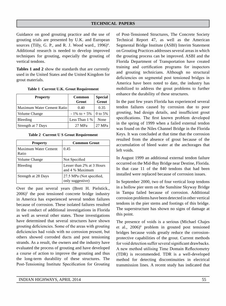
TeCHNICAl pApeRs
INDIAN HIGHWAYS, APRIL 2014 55
Guidance on good grouting practice and the use of grouting trials are presented by U.K. and European sources (Tilly, G. P., and R. J. Wood ward., 1996)4. Additional research is needed to develop improved techniques for grouting, especially the grouting of vertical tendons.
Tables 1 and 2 show the standards that are currently used in the United States and the United Kingdom for grout materials.
Table 1 Current u.K. Grout Requirement
property Common Grout
special Grout
Maximum Water Cement Ratio 0.40 0.35Volume Change - 1% to + 5% 0 to 5%Bleeding Less Than 1 % NoneStrength at 7 Days 27 MPa 27 MPa
Table 2 Current u s Grout Requirement
property Common GroutMaximum Water Cement Ratio
0.45
Volume Change NotSpecifiedBleeding Lesser than 2% at 3 Hours
and 4 % MaximumStrength at 28 Days 27.5MPa(Notspecified,
only suggestive)
Over the past several years (Brett H. Pielstick., 2006)5 the post tensioned concrete bridge industry in America has experienced several tendon failures because of corrosion. These isolated failures resulted in the conduct of additional investigations in Florida as well as several other states. Those investigations have determined that several structures have shown groutingdeficiencies.Someoftheareaswithgroutingdeficiencieshadvoidswithnocorrosionpresent,butothers showed corroded ducts and post tensioning strands. As a result, the owners and the industry have evaluated the process of grouting and have developed a course of action to improve the grouting and thus the long-term durability of these structures. The Post-Tensioning Institute Specification for Grouting
of Post-Tensioned Structures, The Concrete Society Technical Report 47, as well as the American Segmental Bridge Institute (ASBI) Interim Statement on Grouting Practices addresses several areas in which the grouting process can be improved. ASBI and the Florida Department of Transportation have created training and certification programs for inspectorsand grouting technicians. Although no structural deficiencies on segmental post tensioned bridges inAmerica have been noted to date, the industry has mobilized to address the grout problems to further enhance the durability of these structures.
In the past few years Florida has experienced several tendon failures caused by corrosion due to poor grouting, bad design details, and insufficient groutspecifications. The first known problem developedin the spring of 1999 when a failed external tendon was found on the Niles Channel Bridge in the Florida Keys. It was concluded at that time that the corrosion resulted from the absence of grout because of the accumulation of bleed water at the anchorages that left voids.
In August 1999 an additional external tendon failure occurred on the Mid-Bay Bridge near Destine, Florida. In that case 11 of the 840 tendons that had been installed were replaced because of corrosion issues.
In September 2000, two of four vertical loop tendons in a hollow pier stem on the Sunshine Skyway Bridge in Tampa failed because of corrosion. Additional corrosion problems have been detected in other vertical tendons in the pier stems and footings of this bridge. The superstructure has shown no signs of damage at this point.
The presence of voids is a serious (Michael Chajes et al., 2006)6 problem in grouted post tensioned bridges because voids greatly reduce the corrosion-protective capabilities of the grout. Current methods forvoiddetectionsufferseveralsignificantdrawbacks.AnewmethodutilisingTimeDomainReflectometry(TDR) is recommended. TDR is a well-developed method for detecting discontinuities in electrical transmission lines. A recent study has indicated that

TeCHNICAl pApeRs
56 INDIAN HIGHWAYS, APRIL 2014
TDR can be used as an effective nondestructive damage detection method for concrete bridges. A void changes the electrical properties of transmission lines and therefore introduces electrical discontinuities. It can be detected and analysed by TDR. Experiments on short specimens that are used to model grouted post tensioning ducts with built-in voids have been conducted and demonstrated the potential of TDR as a void detection method.
Non-destructive Evaluation Method for Determination (Larry D. Olson., 2008)7, of Internal Grout Conditions inside Bridge Post-tensioning Ducts using Rolling Stress Waves for Continuous Scanning”. Post-tensioned systems have been widely used for infrastructure bridge transportation systems since late 1950s. However, if a good quality control plan is not implemented during construction, there is the potential problem during construction that the ducts which carry the post tensioning cables may not be fully grouted. This results in voids in some areas therefore insufficient protection for post-tensioningsteel tendons. Over the long term, water can enter the tendon ducts in the void areas resulting in corrosion of the tendon. The collapse of a two bridges in UK and a corrosion related failure in a bridge in Florida have shown that it is important to have a reliable method to practically inspect the quality of grout fill insidethe ducts after the grouting process is complete. It is equally important to be able to evaluate the condition of older bridges which were never inspected for voids.
ASTM recommended following guidelines for grouting as mentioned below:
● ASTMC939“StandardTestMethodforFlow of Grout for Replaced-Aggregate Concrete (Flow Cone Method)”8
● ASTM C 942 – 99 “CompressiveStrength of Grouts for Preplaced-Aggregate Concrete in the Laboratory1-Designation”9
● ASTM: C 940 – 98 “A Standard TestMethod for Expansion and Bleeding of
Freshly Mixed Grouts for Preplaced-Aggregate Concrete in the Laboratory”10
● ASTM:C953–87(Reapproved1997)“Standard Test Method for Time of Setting of Grouts for Preplaced-Aggregate Concrete in the Laboratory”11.
The purpose of grouting is to provide (MORT&H, 2001)12 permanent protection to the post tensioning steel against corrosion and develop bond between steel and surrounding structure. The compressive strength of 100 mm cube of the grout at 7 day should not be less than 17 MPa.
2.2 Quality Control
Grouting is the primary protection for the post tensioning system. Proper supervision and the use of a bleed-resistant grout that is properly mixed and injected into the tendon are all integral parts of a successful grouting operation. The durability of the structure is directly affected by the grouting operation. Prior planning with the proper details and training of grouting technicians are keys to a successful project.
2.2.1 Grouting Preparation
Before the installation of tendons all (Schokker A. J., B. D., et. al., 1999)13 open ducts should be sealed to avoid contamination from the elements as well as during transport. When the tendon is installed and stressed, the grout caps should be placed as soon as the elongations have been approved and the tails of the tendon have been cut. This is done to keep any possible construction debris or contamination from entering the duct system.
The grout manufacturer’s recommendations for mixing and pumping of the grout must be followed. The over- or under mixing of grout can compromise the consistency and density of the grout and can add toomuchortoolittlewater.Groutflowinthetendonshould be in one direction starting from the lowest part and progressing along the tendon. This requires that the sequences for the use of inlets and outlet vents be welldefined.Contingencies shouldbeaddressed forblocked tendons or crossover. With corrective actions

TeCHNICAl pApeRs
INDIAN HIGHWAYS, APRIL 2014 57
in place and in the plan, a repair ormodified groutprocedure can proceed, making a potential problem a no problem.
2.2.2 Materials and Grouting Operations
Before the grout is pumped, each duct should be tested for leaks. This can be done with oil-free compressed air or potable water. If leaks are found, they should be sealed before grouting to prevent blockages due to partially filled ducts. This procedure will detectcrossover or blockage problems within the system. A crossover results when grout physically crosses between two adjacent post tensioning tendon ducts or enters a duct that was not intended to be grouted at that time, resulting in serious problems if it is not detected before grouting. As any delay to the grouting operation can cause problems and potential delays to the project, it is important that, once a problem is detected, repairs to be made before grouting. If the groutdoesnotflowcorrectlyand freely through thesystem, the integrity of the grouting will be in question. In an effort to provide a more consistent grout material, Florida DOT is requiring the use of a prebagged bleed-resistant grout. ASBI and PTI have recommended the use of antibleed or low-bleed grouts that meet a series of performance requirements. These grouts reduce the size and the number of voids due to bleed water. Although all of these grouts need to be mixed at the proper water–cement ratio with the right equipment. The type of mixer and the time that the grout is mixed are factors that determine the quality of the grout. The manufacturer’s instructions should be followed, and a colloidal or shear-type mixer should be used to obtain a homogeneous mixture. Over mixing of the grout will result in a variable density grout, whereas under mixing of the grout will produce an inconsistent poorgrout.Groutshouldflowfromtheinjectionpointto thefirst vent,with any residualflushingwaterorentrapped air removed. That vent should then be closed. The remaining vents should be closed in sequence in thesamemanner.Thiswillprovideacontinuousflowof grout throughout the grouting operations. Changes in the material requirements for the high-density polyethylene duct systems have been suggested for all
external post tensioning system (Schokker A. J., B. D..et.al., 1999)12.
2.2.3 Training
From the problems observed in Florida, the training of grout personnelwas identified as one of the keycomponents to a good grouting job. The grout foremen, inspectors, and supervisors must be competent and knowledgeable in correct grouting.
2.2.4 Inspection Requirements
The trainingofgrout technicianswas identifiedasakey component to achieving an adequate grouting job. The use of construction inspectors can improve the quality of the grout operation. The inspector should keep records of the tendons that have been grouted, the date of grouting, flow rates, the lot numbersfor prebagged grout mixes, and all other pertinent information. The inspector and the Contractor shouldperformfluidityanddensitytestingtoensurethat the theoretical properties of the grout meet the project specifications. Inspectors should work withthe contractor when performing any remedial action needed during the grouting operation to provide the highest quality possible.
3 mAJoR FINDINGs
Based on available literatures, following major points are highlighted:
● Groutprotectsstrandfromcorrosion;
● Ductshouldbefreefromair
● Tendon failure occurred abroad due tocorrosion of strand;
● Proper training, supervision guidanceare required for good quality control of grout;
● Verylimitedresearchworkcarriedouttodetermine void in grouting duct; and
● IRC specification recommended verylimited tests for the quality control of grout.

TeCHNICAl pApeRs
58 INDIAN HIGHWAYS, APRIL 2014
4 obJeCTIVe AND sCope oF pReseNT ReseARCH WoRK
Based on available literatures, major findings anddraw back of IRC practices, importance of grouting in post tensioning system and needs of present works, following quality control tests are identifiedconsidering international practices:
● Sievetest ● Fluidity; ● Bleeding ● Volumechange; ● Strength; ● Settingtime; ● Fluiddensity.
5 eXpeRImeNTAl TesT seT up
5.1 materials for Grout
5.1.1 Cement
Ordinary Portland cement, Grade 53 has been used. The physical and chemical properties were tested and testresultsarefoundwithinspecificationlimits.Someimportant test results are shown in Table 3.
Table 3 Chemical and physical properties of Cement
Chemical propertiesRatio of Alumina to Iron Oxide 1.56Insoluble residue 2.40Total loss on Ignition 2.22Chloride content 0.018
physical propertiesConsistency 28 %Fineness 3.3 %Initial and Final Setting Time 120 & 190 minutes Cube Strength (7.5 cm cube) 33,43 and 59 MPa
5.1.2 Sand
YamunaNagarsandisused.Thesandzone,finenessmodulus,specificgravityandwaterabsorptionweretested and test results reported in Table 4.
Table 4 properties of sand
Test ResultSand Zone Zone IIFineness Modulus 2.920SpecificGravity 2.822Water Absorption 1.18 %
5.1.3 Water
Locally available water is used for preparation of cube mould and water is tested as Per IS: 456:2000 and test results are shown in Table 5.
Table 5 Test Results of Water
Characteristic Result limitOrganic 20 200 mg/litreInorganic 246 3000 mg/litreSuspended Material 110 400 mg/litreSulphate 125 3000 mg/litreCholoride 25 2000 mg/litre
5.1.4 Admixture
BASF Rehoubuid 819 RM was used and chemical properties were tested and test results are shown in Table 6.
Table 6 properties of Admixture
Test ResultPH value 7.74Dry Material Content 38.91 %Density 1.226 g/ccChloride 0.0036 %Ash Content 7.1 %
5.2 brief Description of Tests
5.2.1 Sieve Test
Grout is passing 150 micron sieve and report the presence of lump in the sieve.
5.2.2 Fluidity
Thefluidityofthegroutduringtheinjectionperiodismeasured using grout spread method.

TeCHNICAl pApeRs
INDIAN HIGHWAYS, APRIL 2014 59
5.2.3 Bleeding
Thebleedingofthegroutissufficientlylowtopreventexcessive segregation and sedimentation of the grout materials. Bleeding is tested by the wick induced method and average of three results the bleeding is reported and value not exceed 3% of the initial volume of the grout after 3 hours kept at rest.
5.2.4 Volume Change
The volume change is determined by wick method. The volume change of the grout is tested for 24 hours and reported within the range of 0% and + 5%.
5.2.5 Strength
The compressive strength of grout assessed at 7 days with cube size of 100 mm.
5.2.6 Setting Time
Setting time of grout is determined with Vicat Apparatus complying with the following:
Initialsetofthegrout;≥3h.
Finalsetofthegrout;≤24h.
5.2.7 Density
Fluid density is measured using known volume of pot and reported density in g/cc.
5.3 Test Frequency
The following test frequency shown in Table 7 is proposed.
Table 7 Recommended Testing of Grout for per Day Work
property Test method Frequency of TestHomogeneity Sieve Test OneFluidity Grout Spread One test immediately and two tests after 30 minutesBleeding WickInduced Two testsVolume Change WickInduced Two testsSetting Time One testDensity Weight to Volume Two testsCompressive Strength 100 mm cube One test at 7 Days (Three Cubes) for upto 5 m3 grouting,
two test for 6-15 m3 grouting
5.4 equipment and Testing procedure
5.4.1 Sieve Test
The test consists of pouring a quantity of grout through a sieve to check for the absence/presence of lumps on the sieve
Apparatus
A150mmdiametersievewithanaperture≤2mm.
Procedure
Pour a minimum of one litre of freshly mixed grout through the sieve.
Reporting
Report the absence/presence of lumps on the sieve.
5.4.2 Fluidity Test
Fluidity test has been carried out by grout spread method.
5.4.2.1 Grout Spread Method
Principle of test
The grout spread test measures the fluidity ofthixotropic grouts. The fluidity is measured by thediameter of the circle of grout spread on a smooth plateafterafixedperiodof30seconds.
Apparatus
The following apparatus is used for this test:
a) Glass or polished steel plate with a minimum diameter of 300 mm.

TeCHNICAl pApeRs
60 INDIAN HIGHWAYS, APRIL 2014
b) Stiff mould made of steel or plastic with an internal diameter of 39 mm and a height of 60 mm.
c) Stopwatch showing time to 0,1 s. d) Thermometer. e) Ruler with a minimum length of 300 mm
with 1 mm graduation.
Test procedure
Preparation
The spread test is carried out on the horizontal plate. Ensure that the surfaces of the mould and plate are clean and slightly moistened. If necessary apply a thinfilmofpetroleumjelly(e.g.Vaseline)tothebrimof the mould in contact with the plate to prevent the mouldfromleakingduringfillingwithgrout.
Procedure
Place the mould on the plate and prevent it from sliding. Pour the grout slowly into the mould until the level of the grout has reached the upper brim. The mould is steadily lifted from the plate and kept above the spread for a maximum of 30 s before it is taken away. The spread is measured in two perpendicular directions at 30 s after the start of lifting the mould.
Reporting of results
Report the spread diameter as the average measured in the two perpendicular directions across the grout spread in millimeters.
Fig. 1 Grout Spread Test
1 – Cylinder (steel or plastic tube)
2 – Smooth plate
5.4.3 Bleeding and Volume Change Test
This test has been carried by Wick-induced test method.
5.4.3.1 Wick-Induced Test
Principle of test
This test provides both volume change and bleeding measurements. Bleeding is measured as the volume of water remaining on the surface of the grout which has been allowed to stand protected from evaporation.
The volume change is measured as a difference in percentage of the volume of grout between the start and the end of the test. The volume change is to be observed after 24 hrs under bleeding volume change.
Equipment
One transparent tube, of approximately 70 mm internal diameter, and approximately 1 m long, equipped with caps at each end.
One 7-wire strand approximately 900 mm long which fitsinsidethetubeandthermometer.
Procedure
Set up tube in a vertical position with its open end at thetop.Providerigidfixingsothatnomovementorvibration can occur. Install the strand inside the tube as shown in Fig. 2,ensuringthatitisfirmlylocatedonthe base, and held centred. Pour the grout into the tube atasteadyflowratetoensurethereisnotrappedair.Fill the tube to a height, ho, about 10 mm above top of the steel. Seal top of tube to minimise evaporation. Record the temperature of the grout and ambient air temperature.
Record starting time t0 and height h0 of the grout. Record height of grout, hg,at15minintervalsforfirsthour and subsequently at 2h, 3h and 24h.
Record height of bleed water, hw, at the same times as for the grout (see Fig. 2). Record in homogeneities that may develop in the appearance of the grout as seen through the transparent tube. Examples of in homogeneities are:
● formationoflensesofbleedwaterbelowtop of grout;

TeCHNICAl pApeRs
INDIAN HIGHWAYS, APRIL 2014 61
● Segregationsleadingtoareasofdifferentcoloured grout.
Reporting of results
Bleeding is expressed as :
hw/ho x 100%
Volume change is expressed as:
(h0 – hg)/ho x 100%
Fig. 2 Wick-Induced Test Set-Up
5.4.4 Compressive Strength Test
Cubes of 100 mm size have prepared for testing. Cubes were cured in a moist atmosphere for first 24 hours and subsequently in water.
The compressive testing was tested in compressive testing machine at 7 days and measured on at least three specimens.
Reporting of results
The average of all results of the compressive cubes expressed, in N/mm2.
5.4.5 Density Test
The density is measured as the ratio of mass to volume inthefluidstate.Theapparatuscomprisescalibratedequipment for weight and volume measurement.
Reporting of results
The method of sampling, measuring weight and volume, the equipment used and the density determined is reported in g/cc.
5.4.6 Air Void Detection Test
An indirect method is proposed. Theoretical volume of duct has to be estimated. The actual volume of grout is calculated by adding certain percentage of theoretical volume for accounting leakage to the theoretical volume. This theoretical volume is compared with the actual volume of grout used to the grout cable. Whenthegroutstartsflowingfromotherend,itshallbeallowedtoflowforoneminute.Afteroneminutethe outlet is closed and the pressure is allowed to build up to 0.5 MPa. This pressure is maintained for one minute and then the operation shall be stopped and the actual consumption of the grout used in the operation shall be estimated and compared with theoretical volume. This is an in accurate method and it does not ensure the actual condition of grouting. Hence this method should be updated/replaced with the latest development taken place in the developed countries. Following methods are proposed:
● Endoscope, ● PressureVacuum, ● Radiology, ● Percussive, ● DiamondCoreDrilling, ● HighPressureWaterJetting, ● GritBlastedHole, ● Radar,
The methods of void detection can be non destructive and a guide line mentioned in B S 1881-201, 198614 shall be used.
5.5 mix Design
Mix design is prepared using cement, water and admixture.
Cebex 100 is used as Cementitious grout admixture.

TeCHNICAl pApeRs
62 INDIAN HIGHWAYS, APRIL 2014
Mix design has been finalized by trial and errormethod. Water cement ratio was found 0.37.
Cebex 100 is used 0.45% eight of cement as declared by the manufacturer.
Plasticizer is used as 0.3% weight of cement as declared by the manufacturer.
Flow found 165 mm initially and 155 after 30 minutes and Bleeding found 0%. Flow in Marsh cone was found 9.4 seconds initially and 9.9 seconds after 30minutes.Detailtrialforfinalizationofmixdesignis shown in Table 8.
7 days cube (100 mm size) was found 36.9 MPa > 17 MPa.
All materials have been batched by mass. The accuracy ofbatchingwas0 ±2%forcement,dryadmixturesand 0 ± 1 % for water and liquid admixtures, of the quantities specified. Water contained in liquidadmixtures is included in the calculation of W/C ratio.
All pozzolanic materials used as separate ingredients are included in the calculation of W/C ratio.
Mixing has been carried out mechanically with suitable equipment to obtain a homogeneous and stable grout with the plastic properties.
Following information are declared by the grout manufacturer:
● Mixproportionsofmaterials: ● W/Cratioanditsacceptabletolerance; ● Sequence of introducing the materials,
type of mixer and mixing time; ● Rangeoftemperatureforwhichthegrout
complies with the European standard.
5.6 Test Results
Test results are found satisfactory. Summary of the test results mentioned in Table 8.Volume change in all tests is found zero. Other test results are reported in Table 8.
Table 8 summary of Test Results
s. No. W/C Ratio
Cement Content
in g
Cebex 100 in g
super plasticizer
in g
sieve Test
Density (g/cc)
Water in g
Flow in mm marsh Cone Flow in sec
bleeding at 3 h in
%
Compressive strength at 7 Days in
mpaInitial After 30
minutesInitial After 30
minutes
1 0.45 2000 9 4.96 0 2.010 900 225 200 6.37 8.4 4.76 28.5
2 0.44 2000 9 5.208 0 2.002 880 215 195 8 9.1 3.61 29.6
3 0.43 2000 9 5.456 0 1.993 860 210 190 7.4 8.8 3 31.6
4 0.42 2000 9 5.952 0 1.981 840 200 185 8.2 9.1 2.9 33.1
5 0.41 2000 9 6.448 0 1.970 820 195 175 8.6 9 2.6 33.6
6 0.4 2000 9 6.944 0 1.962 800 185 175 8.9 9.2 1.4 34.1
7 0.39 2000 9 7.192 0 1.955 780 178 170 9.1 9.6 1 34.5
8 0.38 2000 9 7.44 0 1.949 760 170 165 9.3 9.8 0.8 36.1
9 0.37 2000 9 7.44 0 1.941 740 165 155 9.4 9.9 0 36.9
6 CoNClusIoNs AND ReCommeNDATIoNs
6.1 Several design details have been changed to improve the characteristics and performance of the post tensioning systems.6.2 Several changes to the grout material have been recommended. The use of antibleed or no-bleed grouts is recommended.
6.3 Improvement of the grout equipment will provide a consistent mix and uniform density for the grout.
6.4 Itisrecommendedthattrainingandcertificationfor grouting technicians and inspectors be required. Government agency will be authorized to conduct such training.

TeCHNICAl pApeRs
INDIAN HIGHWAYS, APRIL 2014 63
6.5 New code to be developed/Specification ofpresent IRC needs to be revised including void detectionmethodologytobeidentified.
6.6 No bleeding grout is to be used for better quality control and longer life span of post tensioning structure.
ReFeReNCes1. Woodward, R. J. Collapse of a Segmental Post-Tensioned
Concrete Bridge. In Transportation Research Record 1211, TRB, National Research Council, Washington, D.C. 1989, pp. 38–59.
2. Clark, L. Performance in Service of Post tensioned Concrete Bridges. Report. British Cement Association, Crowthorne, Berkshire, UK,October 1992.
3. AASHTO (2008), “AASHTO LRFD Bridge Construction Specifications,InterimRevision”pp.10-25.
4. Tilly, G. P., and R. J. Woodward. Development of Improved Grouting for Post tensioned Bridges. In FIP Symposium on Post tensioned Concrete Structures, Vol. 1, 1996, pp. 55–64.
5. Brett H. Pielstick, “Grouting of Segmental Post Tensioned Bridges in America”, TRB 1813,2006, Page, 235-241.
6. Michael Chajes, Robert Hunsperger, Wei Liu, Jian Li, and Eric Kunz,” Time Domain Reflectometry for Void
Detection in Grouted Post tensioned Bridges”, TRB, 1845, 2006, Page 148-152.
7. Larry D. Olson,” Applications and Limitations of Impact-Echo Scanning for Void Detection in Post-Tensioned Bridge Ducts”,TRB,2008,Annual Meeting,CD ROM.
8. ASTM C 939 “Standard Test Method for Flow of Grout for Preplaced-Aggregate Concrete (Flow Cone Method)”
9. ASTM C 942 – 99 “Compressive Strength of Grouts for Preplaced-Aggregate Concrete in the Laboratory1-Designation”.
10. ASTM:C 940 – 98 “A Standard Test Method for Expansion and Bleeding of Freshly Mixed Grouts for Preplaced-Aggregate Concrete in the Laboratory”.
11. ASTM : C 953 – 87 (Reapproved 1997) “Standard Test Method for Time of Setting of Grouts for Preplaced-Aggregate Concrete in the Laboratory”.
12. MinistryofRoadTransportandHighway.“Specificationfor Roads and Bridges”, Indian Roads Congress, 2001.
13. Schokker A.J., B.D. Koester, J.E. Breen, and M.E. Kreger. Development of High Performance Grouts for Bonded Post-Tensioned Structures. Research Report 1405-2. Center for Transportation Research, University of Texas at Austin, Oct. 1999.
14. BS 1881-201, 1986, “Testing Concrete-Part 201-Guide to the Use of Non-destructive method of test for hardened concrete”.
Annexure 1 Different Tests and Specification
property Test Value Test method
Total Chloride Ions Max. 0.08% by weight of cementitious material
ASTM C 1152/C1I52M
Fine Aggregate (if utilized) Max. Size<No. 50 Sieve ASTM C 33
Volume Change at 28 days 0.0% to +0.2% at 24 h and 28 days ASTM C 1090*
Expansion <2.0% for up to 3 h ASTM C 940
Compressive Strength 28 day (average of 3 cubes)
>6 ksi ASTM C 942
Initial Set of Grout Min. 3 h Max. 12 h
ASTM C 953
FluidityTest**EffluxTimefromFlowConea) immediately after Mixingb) 30 min after Mixing with Remixing for 30s
Min. 11sMax. 30s or
Min. 9sMax. 20 s
ASTM C 939ASTM C 939***
ASTM C 939ASTM C 939***

TeCHNICAl pApeRs
64 INDIAN HIGHWAYS, APRIL 2014
property Test Value Test method
Bleeding at 3 h Max. 0.0% ASTM C 940****
Permeability at 28 days Max. 2500 coulombs at 30 volts for 6 h
AASHTO T 277 (ASTM C 1202)
* ModifyASTMC1090toincludeverificationatboth24hand28days.
** AdjustmentstoflowrateswillbeachievedbystrictcompliancewiththeManufacturer’srecommendations.
*** GroutfluidityshallmeeteitherthestandardASTMC939flowconetestorthemodifiedtestdescribedherein.ModifytheASTMC939testbyfillingtheconetothetopinsteadoftothestandardlevel.Theeffluxtimeisthetimetofilla1.0-Lcontainerplaceddirectlyundertheflowcone.
**** Modify ASTM C 940 to conform with the wick induced bleed test described below:
a) Condition dry ingredients, mixing water, prestressing strand and test apparatus overnight at 70 to 77°F.
b) Insert 800 mL of mixed conditioned grout with conditioned water into the 1000 mL graduated cylinder. Mark the level of the top of the grout.
c) Wrap the strand with 2.0-in, wide duct or electrical tape at each end prior to cutting to avoid splaying of the wires when it is cut.
Degrease (with acetone or hexane solvent) and wire brush to remove any surface rust on the strand before temperature conditioning. Insert completely a 20.0-in, length of conditioned, cleaned, ASTM A 416/A 416M seven wire strand 0.5-in, diameter into the 1000 mL graduated cylinder. Center and fasten the strand so it remains essentially parallel to the vertical axis of the cylinder (possibly using a centralizer). Mark the Level of the top of the grout,
d) Store the mixed grout at the temperature range listed above in (a).
e) Measurethelevelofthebleedwaterevery15mmforthefirsthourandhourlyafterwardfor2h,
f) Calculate the bleed water, if any, at the end of the 3-h test period and the resulting expansion per the procedures outlined in ASTM C 940, with the quantity of bleed water expressed as a percent of the initial grout volume. Note if the bleed water remains above or below the top of the grout.
obITuARY
The Indian Roads Congress express their profound sorrow on the sad demise of Late Shri S.K. Garg, resident of B-21, Sarvodaya Nagar, Kanpur (Uttar Pradesh) and Late Shri A.A. Salam, resident of E-2, Ullas Nagar, Peroorkada, Trivandrum, Kerala. They were very active members of the Indian Roads Congress.
May their souls rest in peace.

INDIAN HIGHWAYS, APRIL 2014 65
Is bus FARe THe oNlY CoNCeRN To uRbAN TRIp mAKeRs’? AN eXpeRIeNCe IN KolKATA
sauraBh dandaPat*, BhargaB maitra** and c.v. PhaniKumar***
* Research scholar, E-mail: [email protected]** Associate Professor, E-mail: [email protected]*** Accent Fellow, Institute for Transport Studies, University of Leeds, Leeds, UK. LS2 9JT E-mail: [email protected]
AbsTRACTAlthough bus is the predominant public transport mode, the quality of bus service is extremely poor in almost all Indian cities. The poor quality of bus service along with economic progression is leading to rapid growth of private vehicle ownership and usage in urban areas. Historically, the bus fare has been considered as the only socio-political concern in urban India without any emphasis on the quality of service. The paper presents an investigation on the perception of trip makers towards quantitative and qualitative attributes of bus system in the Kolkata metro city. A stated choice experiment was design and the data collected from trip makers were analyzed by developing Multinomial Logit and Random Parameter Logit models. The willingness-to-pay values were also calculated in order to understand the perception of trip makers towards bus service attributes. The results indicate that the fare is not the only concern to trip makers. The work justify the need for improving the overall quality of bus service to enhance the attractivenessofbussystemandthebenefittobususers.
1 INTRoDuCTIoN
Bus is the predominant public transport mode in majority of Indian cities. But, the quality of bus service is extremely poor in almost all cities. The poor quality of bus service along with economic progression is leading to rapid growth of private vehicle ownership and usage in urban areas. On the other hand, the scope of capacity augmentation of roads in most of the cities is limited due to non-availbility of land. As a result, there is a growing imbalance between the demand and the supply of transport in urban areas. The growing imbalancehasnotonlyaggravatedtrafficcongestionbut also increased vehicular emissions.
Bus system has the potential to work as an effective instrument for demand management in urban areas. Higher bus usage can reduce vehicle volumes and
thereby bring down traffic congestion and vehicularemissions. In fact the role of public transportation system in urban areas has been recognised in National Urban Transport Policy (NUTP 2006). Accordingly, several initiatives have been taken by the Govt. of India and various State Governments to increase the supply of buses(1 & 2). For example, Govt. of India initiated JnNURM scheme(3) which has added nearly 15000 buses in 61 cities in India. But, the overall poor quality of bus service in urban India is yet to change significantly.
In the context of bus service, the fare remained as the only sociopolitical concern. There has been frequent discussions about the bus fare in public domain without any emphasis on the quality of service. It would have been ideal to have a high quality bus service in urban India with a low fare. But, in reality most of theGovernments arefinding it increasinglydifficulteven to sustain the existing subsidies on bus transport. Constraints on subsidy and fare have adversely affected the quality of bus service in urban India. In most cases, quality of vehicle is poor, journey time is long, traffic information isabsent,anddiscomfortdue to overcrowding is high. However, practically adequate investigation has been done in Indian context to understand if the fare is the only concern to urban tripmakers or the overall quality of bus service is also an important consideration. The present work reports an investigation on perception of urban trip makers towards various bus service attributes. The perception of tripmakers towards bus service attributes has been captured in terms of their Willingness-To-Pay (WTP). The work is demondtrated with reference to a case study of Kolkata metro city.
Civil Engineering Department, Indian Institute of Technology, Kharagpur, W.B. India

TeCHNICAl pApeRs
66 INDIAN HIGHWAYS, APRIL 2014
2 meTHoDoloGY
2.1 Approach
Revealed Preference (RP) and/or Stated Preference (SP)datahavebeenusedextensivelyindiversefieldsfor valuation of attributes or estimation of WTP values(4-7). However, RP data can not accommodate non-existing parameters and fail to represent variability of attributes which in-turn does not permit to establish their influences in the model. On theother hand, a systematic combination of levels of each attribute may be considered in SP experiments(8). Besides, it requires comparatively less number of observations and also facilitates inclusion of hypothetical attributes and variability of attributes. Moreover, SP models are well established and have been used extensively for calculating marginal WTP values(9 & 10). Therefore, in the present work SP data are used for calculating trip makers’ WTP with respect to various attributes of bus system in the Kolkata metro city.
Some of the SP studies have used ranking or rating-based techniques(11). But, these techniques lack strong theoretical foundation consistent with economics(12). As a result, it may not be able to capture the true choice behavior of respondents. In addition, potential theoretical and practical obstacles in ranking and rating techniques lead to difficulty in makinginterpersonal comparisons and departure from the choice contexts that are faced by consumers in the real world(13). On the other hand, the Discrete Choice Experiment (DCE) provides a framework for estimating relative marginal disutility of variations attributes, and their potential correlations(14). The method involves consumers, making mutually exclusive choices from a set of substitutable alternative. Moreover, DCE is an established approach with strong theoretical foundation based on economic theory, for understanding and predicting consumer tradeoffs and choices in marketing research. DCE method has also been used extensively in the fieldof transportation for modeling individual’s behavior in various contexts such as valuing travel time
savings(8 & 15-17), mode choice(18 & 19), route choice(20), vehicle choice(21), etc. Therefore, the DCE technique is adopted in the present work for collecting the preferences of users’ in the Kolkata metro city.
SP data may be analyzed by different econometric modelspecifications.Inthepresentstudy,itisaimedto understand trip makers perception towards various attributes of bus service. Therefore, the data have been analyzed by developing Multinomial Logit (MNL) and Random Parameter Logit (RPL) models.
2.2 econometric model
The theoretical foundation of MNL and RPL models have been documented in various literatures(18, 22-24). However, a brief outline of these two model specifications are included below in thecontext of the present work.
The MNL models are developed on the basis of Random Utility Theory, where the utility of each element includes an observed (deterministic) component (V) and a random (indeterministic) component(ε):
U=V+ε ...(1)
If the deterministic part ‘V’ is a function of the observed attributes (z) of the choice as faced by the individual, the observed socioeconomic attributes of the individual (S)andavectorofparameters (β),then
V=V(z,S,β) ...(2)
A probabilistic statement can be made (due to presence of the random component) as, when an individual “n” is facing a choice set, Cn, consisting of Jn choices, the choice probability of alternative ‘i’ is equal to the probability that the utility of alternative “i,” Uin, is greater than or equal to the utilities of all other alternatives in the choice set.
For example:
Pn (i) = Pr (Uin≥Ujn, for all j € Cn)
Pn (i) = Pr (Vin+εin≥Vjn+εjn, for all j € Cn,j≠i)

TeCHNICAl pApeRs
INDIAN HIGHWAYS, APRIL 2014 67
Assuming IID (Gumbel distribution) for ε, theprobability (Pn) that an individual chooses ‘i’ can be given by the MNL model:
... (3)
This model can be estimated by Maximum Likelihood techniques. MNL model have some limitations such as Independence of Irrelevant Alternatives (IIA) property and Independently and Identically Distributed (IID) property.
A Random Parameter Logit Model (RPL) was introduced to overcome the limitations of traditional Multinomial Logit Model (MNL). It is used to account for unobserved heterogeneity. In RPL, when an individual ‘n’ is facing a choice set Cn, the utility function of alternative ‘i’ for individual ‘n’ be(16):
i = 1, 2, …., m; n = 1, 2, ……, m ... (1)
Thus,eachindividual’scoefficientvectorβ is the sum of the population mean βI and individual deviation β βn n inX . are error components that persuade heteroskedasticity and correlation over alternatives in the unobserved portion of the utility. εin representsunobserved factors that affect Uin.
Let,tastesβ,varyinthepopulationwithadistributiondensity f (β | θ), where θ is a vector of the trueparameters of the taste distribution. If the error terms (εin)areIID(Independentandidenticallydistributed)type-I extreme value, it is a random parameter logit model(25). The conditional probability of observing a sequence of choices is given by the product of the conditional probabilities:
... (2)
Where, k (n,t) denotes the sequence of choices from choice sets that an individual ‘n’ chooses in situation ‘t’. In the choice experiment, the sequence of choices is the number of hypothetical choices each respondent makes in the survey. The unconditional probability for a sequence of choices for individual ‘n’ is then
expressed as the integral of the conditional probability inthefollowingequationoverallvaluesofβ:
... (3)
In general, the integral cannot be evaluated analytically, and one has to trust on a simulation method for the probabilities. In RPL method, a simulated maximum likelihood estimator, using Halton draws is used. This type of random parameter model is less restrictive than standard conditional logit models. However, care should be taken for application of these less restrictive models.Apart frombeingmoredifficult toestimate,the literature shows that the results can be rather sensitive to the distributional assumptions and the number of draws applied in the simulation(8).
In the present paper, marginal WTP values associated with various bus attributes are estimated using MNL and RPL models.
3 suRVeY INsTRumeNT AND sTuDYA stated choice survey instrument was designed for collecting respondent’s trip characteristics, socioeconomic characteristics, and stated preference ‘choice’ from the choice sets. The survey instrument includedthreeparts.Thefirstpart(PartA)wasdesignedwith the objective of collecting respondent’s trip and socioeconomic characteristics. The trip characteristics were captured in terms of frequency of using bus, type of bus predominantly used and the details of the most recent trip including trip purpose, trip length and fare. On the other hand, the socioeconomic characteristics were captured in terms of age, gender, income, car ownership, etc. The second part (Part B) was designed to make respondents familiar about various attributes and their levels used in the stated choice experiment. This part included description as well as photographs and sketches. Photographs were included especially to communicate to respondents about various types of busesand traffic information systemsavailable.Thethird part (Part C) was designed with the objective of collecting respondents’ choice with respect to each choice set. This part included six choice sets with two hypothetical alternative bus service in each set.

TeCHNICAl pApeRs
68 INDIAN HIGHWAYS, APRIL 2014
During preliminary investigation in the Kolkata metro city it was observed that journey speeds for buses were generally very low (about 8 to 15 kmph), buses were crowded and headway was often in the range of 5 to 15 minutes. Also, bus schedules were largely not known to passengers, and no information was available at bus stops or on-board. Presently, the Kolkata city is predominantly served by four distinctly different types of bus called as Mini Bus (BT1), Ordinary Private Bus (BT2), Ordinary State Bus (BT3) and Jawaharlal Nehru National Urban Renewal Mission (JnNURM) Bus (BT4). The dimensions, appearance and comfort offered by these buses are different. The newly introduced JnNURM buses appear to be most attractive in terms of appearance and comfort among all types of bus operating in the Kolkata metro city. Apartfrombusfarefiveattributesofbussystemwereincluded as attributes in the choice experiment. The attributesconsideredinthestudycanbeclassifiedasquantitative attributes and qualitative attributes. The quantitative attibutes included average journey speed, travel cost and waiting time at bus stop. On the other hand, the qualitative attributes included discomfort during journey, type of bus, and nature of trafficinformation. Each attribute was further described by fourorfivelevelsasmentionedbelow:
i) Type of Buses : Mini Bus (BT1), Ordinary Private Bus (BT2), State Bus BT3), JnNURM Bus/Articulated Bus (BT4).
ii) Waiting Time at bus stop ((WT) in minutes): 3, 6, 9, 12, 15.
iii) Comfort Condition Inside vehicle:
● Seat(CC4)
● Standing Comfortably (CC3:number of standee equivalent to 33% of standees under crush load condition)
● Standing in congestion (CC2:number of standee equivalent to 66% of standees under crush load condition)
● Standing at crush load condition(CC1)
iv) Trafficinformation:
● Traditional way of displayingbus route/destination information (TI1)
● Displaying bus route/destinationinformation using LED display (TI2)
● Displaying bus route/destinationinformation using LED display + on-board information using LED display (TI3)
● Displaying bus route/destinationinformation using LED display + on-board information using LED display + LED display at bus stop with bus arrival information (TI4)
v) In-Vehicle Travel Time (IVTT in minutes) based on Average Journey Speed (in km/hour):
● The following levels of averagejourney speed were included.
● For ShortTrips (Up to 6 kmfivelevels): 8, 10, 12, 14, 16
● ForLongTrips(Beyond6kmfivelevels): 10,12,14,16,18
vi) Fare (INR/km)
● For ShortTrips (Up to 6 kmfivelevels): 1.1, 1.4, 1.7, 2.0, 2.3
● ForLongTrips(Beyond6kmfivelevels): 0.5, 0.8, 1.1, 1.4, 1.7
It may be mentioned that although the choice sets included bus journey speed as an attribute, the corresponding journey time was also mentioned during the data collection. A D-optimal design technique was used to produce the choice sets of five blocks eachhaving six paired alternatives. All the alternatives in a

TeCHNICAl pApeRs
INDIAN HIGHWAYS, APRIL 2014 69
choice set were presented in generic form (i.e., Alt-A and Alt-B).
Pilot surveys were carried out in February 2011 in order to identify various important aspects of questionnaire and data collection such as respondents’ understanding level, proper explanation of SC experiment, decision
on the number of choice sets in each questionnaire considering respondents’ fatigue, identification ofvarious strategic locations for intercepting commuters and also for providing a sort of training to the interviewers. Necessary changes were incorporated in the questionnaire based on the pilot studies. A sample of an SP choice set is presented in Fig. 1.
Choice set:-sC1 Type of Bus Waiting
TimeDiscomfort TrafficInformation In-vehicle
travel time Fare (Rs.)
Your Choice
JnNURM/
Articulated bus
15 min Comfortable Standee
LED display outside +onboard
60 min 11.00
Ordinary Private Bus
3 min Congested Standee
LED display outside 33 min 14.00
Fig. 1 Sample Choice Set
During data collection, tripmakers were intercepted at several strategic places in the Kolkata metro city in order to collect their responses. Paper pencil based face-to-face interview the chique was adopted during the survey and the respondents were approached randomly. During the survey, 350 respondents covering different age groups, trip purposes, income levels, etc. were interviewed. Out of the 2100 responses, 1614 refined responses were used formodel development. Other responses were rejected mainly because of incompleteness of information or missing data.
4 DATAbAseThe database included respondent’s socioeconomic characteristics such as age, occupation, personal income, household size, car ownership, occupation, education and household income. It also included trip characteristics such as trip length, purpose, duration of trip, fare paid, and route characteristics such as length of route for the most recent trip. Depending on the trip length, tripswere classified as short trip (≤ 6 Km) or long trip (> 6 km). Out of 1614observations, 930 (58%) responses were collected from male respondents. Summary of trip and socioeconomic characteristics of respondents as per therefineddatabaseisgiveninTable-1.
Table 1 summary of Trip and socioeconomic Characteristics of Respondents
Variable(s) DescriptionTrip Purpose levels Work business education Recration shopping social other
Number 828 173 302 111 66 75 59Household Income per
month (INR)
levels ≤10K 10k-20K 20k-30K 30K-40K 40K-60K 60K-80K >80KNumber 246 583 422 196 105 23 39
Age (Years) levels ≤20 21-35 36-55 >55Number 62 841 600 111
Car ownership (No. of car)
levels 0 1 ≥2Number 1153 398 63

TeCHNICAl pApeRs
70 INDIAN HIGHWAYS, APRIL 2014
5 moDel DesCRIpTIoN, ResulTs AND DIsCussIoN
Keeping in view the objective of present work, the quantitative attributes such as In Vehicle Travel Time, Waiting Time and Fare were entered in the model in cardinal linear form. On the other hand, dummy coding was used for three qualitative attributes such as bustype,trafficinformationandcomfortcondition.InBus type, BT4 was considered as the base alternative. IncaseofTrafficInformation,TI4wasconsideredasthe base alternative and CC4 was considered as the
base alternative for comfort level during travel. Based on these assumptions, model estimation was carried out for all other levels of corresponding attributes.
The MNL and RPL models were developed using LIMDEP 8.0 (Greene 2002). While developing RPL models, a Constrained Triangular (CT) distribution (26) for the random parameters(s) where spread of the random parameter equals its mean, was assumed. The MNL and RPL models developed in the present study are presented in Table 2.
Table 2 Coefficient Estimates from MNL and RPL Models
Attributes mNl Coefficient (t -Stat)
Rpl
Coefficient (t -Stat)IVTT -0.622 (-14.31) -0.745 (-12.21)WT -0.041(-5.00) -0.046 (-4.83)BT1 -0.801 (-4.61) -0.922 (-4.49)BT2 -0.530 (-5.13) -0.608 (-4.94)BT3 -0.394 (-2.57) -0.418 (-2.29)TI1 -0.893 (-8.55) -0.985 (-7.86)TI2 -1.291 (-3.52) -1.462 (-3.21)TI3 -0.798 (-2.19) -0.826 (-2.01)CC1 -1.098 (-8.96) -1.254 (-8.27)CC2 -0.927 (-5.18) -0.982 (-4.66)CC3 -0.494 (-2.43) -0.472 (-1.99)
Fare -0.007 (-5.70) -0.008 (-5.61)ASC 0.099 (1.43)+ 0.106 (1.32)+
# of Observation 1614 1614Log Likelihood Function -790.861 -789.912
ρ2 0.28732 0.28819+t-valuenotsignificant
It may be observed from Table-2thatthecoefficientestimates of all the attributes and levels are statistically significant. The t-values of coefficient estimatesindicate that all these attributes and levels of bus
service are considered as important by trip makers in theKolkatametro city.The sign of each coefficientestimate is also found logical and as per the actual condition of the bus service in the Kolkata metro city.

TeCHNICAl pApeRs
INDIAN HIGHWAYS, APRIL 2014 71
Negative sign associated with in-vehicle travel time and waiting time indicates that as the value of these attributes increases the disutility also increases.
Among four types of bus service, JnNURM buses are considered superior to other three types of bus. It is interesting to note that between Mini Bus (BT1) and Ordinary Private Bus (BT2), the disutility is considered more for Mini Bus (BT1) which is contrary to the conventional belief. The fare for Mini Bus (BT1) is higher as it is assumed to offer a more comfortable journey. The condition of majority of Mini Buses is extremely poor, leg-space is inadequate and traveling as a standee is more inconvenient due to low head room, which may justify the result in the context of the Kolkata metro city. It is also interesting to note that Ordinary State Bus (BT3) is considered superior to Mini Bus (BT1) and Ordinary Private Bus (BT2). The results bring out the images of four types of bus, as perceived by commuters in the Kolkata metro city.
It is interesting to note that TI2 (Displaying bus route/destination information using LED display) is considered as more disutility than TI1 (Traditional way of displaying bus route/destination information) which is apparently not an expected outcome. A further investigation reveals that in JnNURM buses which are presently operating in Kolkata, the font size used in the LED display is small and there are problems associated with the visibility during daytime. Also, in many cases the LED displays are scrolled fast making itdifficultfortripmakerstoreadandunderstandthecontent.Altogether,KolkatausersfindLEDdisplayinits present form as more disutility than TI1 (Traditional way of displaying bus route/destination information). AcomparisonofcoefficientsofTI2(Displayingbusroute/destination information using LED display) and TI3 (Displaying bus route/destination information using LED display + on-board information using LED display) indicates that on-board information using LED display is considered as utility by trip makers. A comparisonofcoefficientestimateofTI3(Displayingbus route/destination information using LED display + on-board information using LED display) with the base alternative clearly indicate that LED display at
bus stop with bus arrival information is also considered as utility by trip makers.
The coeeficient estimates assiciatedwithCC1,CC2and CC3 indicate that crowding inside buses is considered as disutility by tripmakers. Also, more cowding is clearly perceived as more disutility by bus trip makers in the Kolkata metro city.
It may also be observed from Table-2thatthecoefficientestimates obtained from MNL and RPL models are consistent in terms of their interpretations. However, inallcasesotherthanCC3highercoefficientestimatesare obtained from RPL model. In terms of the overall goodness-of-fit (i.e.ρ2),no significant improvementis observed in RPL model. This may be because of the assumption of CT distribution of random parameters in RPL model. No additional parameter is estimated in the present RPL model.
The marginal WTP values are calculated by taking ratioofthecoefficientofeachnon-costattributeandthe coefficient of the cost attribute. The marginalWTP values estimated from MNL and RPL models for various attributes/levels are reported in Table 3. For the qualitative attributes and their levels, WTP values are reported for a shift from the level under consideration to the base level. For example, the WTP for BT2 is for a shift from bus type BT2 to BT4 (base level).
It may be observed that WTP values obtained from MNL and RPL model are generally consistent and comparable. The WTP values clearly indicate that both quantitative and qualitative attributes of bus service are considered as important factors by tripmakers in the Kolkata metro city. The present bus fare in the Kolkata metro city is different for different types of bus service. Also, the fare per km varies depending on the distance travelled. In general, the bus fare per km varies in the range of INR 1.00 to INR 2.00. A comparison of the present bus fare and the WTP values reported in Table-3 clearly indicates that bus fare is not the only concern to trip makers in the Kolkata metro city. Rather, as compared to the fare, trip makers have significant WTP for improvement of various
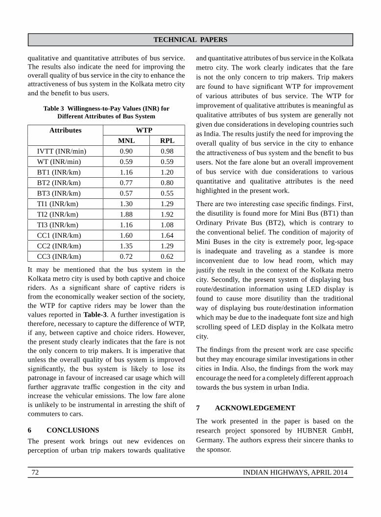
TeCHNICAl pApeRs
72 INDIAN HIGHWAYS, APRIL 2014
qualitative and quantitative attributes of bus service. The results also indicate the need for improving the overall quality of bus service in the city to enhance the attractiveness of bus system in the Kolkata metro city andthebenefittobususers.
Table 3 Willingness-to-pay Values (INR) for Different Attributes of bus system
Attributes WTpmNl Rpl
IVTT (INR/min) 0.90 0.98WT (INR/min) 0.59 0.59BT1 (INR/km) 1.16 1.20BT2 (INR/km) 0.77 0.80BT3 (INR/km) 0.57 0.55TI1 (INR/km) 1.30 1.29TI2 (INR/km) 1.88 1.92TI3 (INR/km) 1.16 1.08CC1 (INR/km) 1.60 1.64CC2 (INR/km) 1.35 1.29CC3 (INR/km) 0.72 0.62
It may be mentioned that the bus system in the Kolkata metro city is used by both captive and choice riders. As a significant share of captive riders isfrom the economically weaker section of the society, the WTP for captive riders may be lower than the values reported in Table-3. A further investigation is therefore, necessary to capture the difference of WTP, if any, between captive and choice riders. However, the present study clearly indicates that the fare is not the only concern to trip makers. It is imperative that unless the overall quality of bus system is improved significantly, the bus system is likely to lose itspatronage in favour of increased car usage which will further aggravate traffic congestion in the city andincrease the vehicular emissions. The low fare alone is unlikely to be instrumental in arresting the shift of commuters to cars.
6 CoNClusIoNsThe present work brings out new evidences on perception of urban trip makers towards qualitative
and quantitative attributes of bus service in the Kolkata metro city. The work clearly indicates that the fare is not the only concern to trip makers. Trip makers are found tohave significantWTP for improvementof various attributes of bus service. The WTP for improvement of qualitative attributes is meaningful as qualitative attributes of bus system are generally not given due considerations in developing countries such as India. The results justify the need for improving the overall quality of bus service in the city to enhance theattractivenessofbussystemandthebenefittobususers. Not the fare alone but an overall improvement of bus service with due considerations to various quantitative and qualitative attributes is the need highlighted in the present work.
Therearetwointerestingcasespecificfindings.First,the disutility is found more for Mini Bus (BT1) than Ordinary Private Bus (BT2), which is contrary to the conventional belief. The condition of majority of Mini Buses in the city is extremely poor, leg-space is inadequate and traveling as a standee is more inconvenient due to low head room, which may justify the result in the context of the Kolkata metro city. Secondly, the present system of displaying bus route/destination information using LED display is found to cause more disutility than the traditional way of displaying bus route/destination information which may be due to the inadequate font size and high scrolling speed of LED display in the Kolkata metro city.
Thefindingsfromthepresentworkarecasespecificbut they may encourage similar investigations in other citiesinIndia.Also,thefindingsfromtheworkmayencourage the need for a completely different approach towards the bus system in urban India.
7 ACKNoWleDGemeNT
The work presented in the paper is based on the research project sponsored by HUBNER GmbH, Germany. The authors express their sincere thanks to the sponsor.

TeCHNICAl pApeRs
INDIAN HIGHWAYS, APRIL 2014 73
ReFeReNCes1. Vaidya, C. (2011), Urban Transport Initiatives in India:
Best Practices in PPP, National Institute of Urban Affairs, The Report submitted to the Ministry of Urban Development, Govt. of India.
2. Urban Initiatives: Peer Experience and ReflectiveLearning (PEARL), (2011). National Institute of Urban Affairs (NIUA), New Delhi, Vol. 5.
3. JNNURM. (2011), JNNURM bus project. Retrieved on 22 June 2011 from http:// www.jnnurm.nic.in/funding-of-buses.html.
4. Phanikumar, C.V. and Maitra, B. (2006), Modeling Willingness-to-Pay Values for Rural Bus Attributes under Different Trip Purposes, Journal of the Transportation Research Forum. Summer, Vol. 45, No. 2, pp. 31-44.
5. Hensher, D. A. (1994), Stated Preference Analysis of Travel Choices: The State of Practice, Transportation, Vol. 21, No. 2, pp. 107–133.
6. Kroes, E.P. and Sheldon, R.J. (1988), Stated Preference Methods: An Introduction, Journal of Transport Economics and Policy, Vol. 22, pp. 11-25.
7. Louviere, J.J. (1988), Conjoint Analysis Modeling of Stated Preferences: A Review of Theory, Methods, Recent Developments and External Validity, Journal of Transport Economics and Policy, Vol. 22, No. 1, pp. 93-119.
8. Hensher, D.A. and Greene, W.H. (2003), The Mixed Logit Model: The State of Practice, Transportation, Vol. 30, Vol. 2, pp. 133-176.
9. Hensher, D.A., Rose, J.M., and Greene, W.H. (2005), Applied Choice Analysis: A Primer, Cambridge University Press.
10. Hensher, D. A. (2007), Sustainable Public Transport Systems: Moving Towards a Value for Money and Network-Based Approach and Away from Blind Commitment, Transport Policy, Vol. 14, No. 1, pp. 98-102.
11. Hunt, J.D. (2001), Stated Preference Analysis of Sensitivities to Elements of Transportation and Urban form, Transportation Research Record: Journal of the Transportation Research Board, Vol. 1780, pp. 76-86.
12. Adamowicz, W., Louviere, J., and Swait, J. (1998), Introduction to Attribute-Based Stated Choice Methods. Report submitted to National Oceanic and Atmospheric Administration, US Department of Commerce.
13. Bennett, J., and Blamey, R.K. (2001), The Choice Modeling Approach to Environmental Valuation, Edward Elgar Publishing Limited, UK.
14. Louviere, J.J., Hensher, D.A., and Joffre, D.S. (2000), Stated Choice Methods. Analysis and Applications, Cambridge University Press.
15. Hensher, D. A. (2001), The Valuation of Commuter Travel Time Savings for Car Drivers in New Zealand: Evaluating AlternativeModelSpecifications,Transportation,Vol.28,pp. 101–118.
16. Greene, W., Hensher, D.A., and Rose, J. (2006), Accounting for Heterogeneity in the Variance of the Unobserved Effects in Mixed Logit Models, Transportation Research, Part B., Vol. 40, pp. 75–92.
17. Hess, S., Bierlaire, M., and Polak, J.W. (2005), Estimation of Value of Travel-Time Savings Using Mixed Logit Models, Transportation Research, Part A, Vol. 39, pp. 221–236.
18. Alpizar, F., and Carlsson, F. (2003), Policy Implications and Analysis of the Determinants of Travel Mode Choice: An Application of Choice Experiments to Metropolitan Costa Rica, Environment and Development Economics, Cambridge University Press, Vol. 8, No. 4, pp. 603-619.
19. Koppelman, F. S., and Sethi, V. (2005), Incorporating Variance and Covariance Heterogeneity in the Generalized Nested Logit Model: An Application to Modeling Long Distance Travel Choice Behavior, Transportation Research Part B: Methodological, Vol. 39, No. 9, pp. 825-853.
20. Yai T., Iwakura, S., and Morichi, S. (1997), Multinomial Probit with Structured Covariance for Route Choice Behaviour, Transportation Research-B, Vol. 31, No. 3, pp. 195-207.
21. Train, K., and Winston, C. (2007), Vehicle Choice Behavior and the Declining Market of us Automakers, International Economic Review, Vol. 48 No. 4, pp. 1469–1496.
22. McFadden, D. (1974), Conditional Logit Analysis of Qualitative Choice Behaviour, In P. Zarembka, ed., Frontiers in Econometrics. New York: Academic Press, pp. 105–142.
23. Bhat, C. (2000), Incorporating Observed and Unobserved Heterogeneity in Urban Work Travel Mode Choice Modeling, Transportation Science, Vol. 34, pp. 228-238.
24. Greene, W. H. (2002), Econometric Analysis, Maxwell MacMillan International Editions, Basic text book.
25. Train, K. (1998), Recreation Demand Models with Taste Differences Over People, Land Economics, Vol. 74, No. 2, pp. 230–239.
26. Phanikumar, C.V. and Maitra, B. (2006), Valuing Urban Bus Attributes: An Experience in Kolkata, Journal of Public Transportation, Vol. 9, No. 2, pp. 69-87.

74 INDIAN HIGHWAYS, APRIL 2014

INDIAN HIGHWAYS, APRIL 2014 75
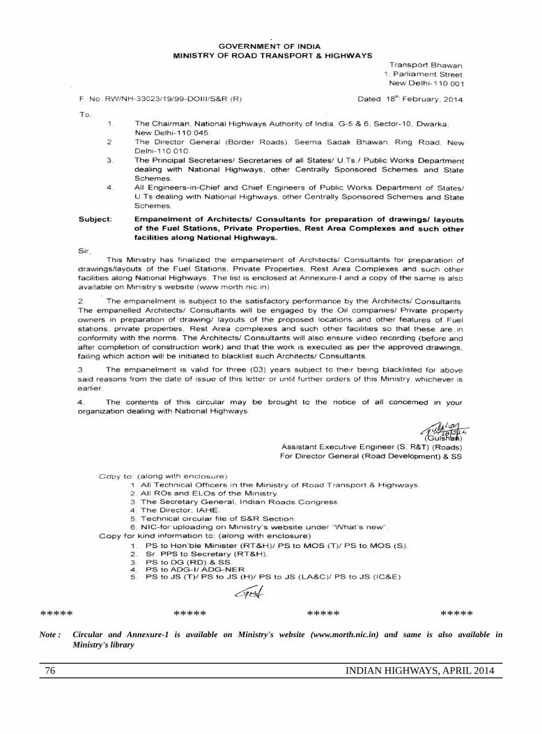
76 INDIAN HIGHWAYS, APRIL 2014
***** ***** ***** *****Note : Circular and Annexure-1 is available on Ministry's website (www.morth.nic.in) and same is also available in
Ministry's library

INDIAN HIGHWAYS, APRIL 2014 77

78 INDIAN HIGHWAYS, APRIL 2014

INDIAN HIGHWAYS, APRIL 2014 79

80 INDIAN HIGHWAYS, APRIL 2014

INDIAN HIGHWAYS, APRIL 2014 81

82 INDIAN HIGHWAYS, APRIL 2014

INDIAN HIGHWAYS, APRIL 2014 83

84 INDIAN HIGHWAYS, APRIL 2014

INDIAN HIGHWAYS, APRIL 2014 85

86 INDIAN HIGHWAYS, APRIL 2014